Does a Big Bazooka Matter? Central Bank Balance-Sheet ...cepr.org/sites/default/files/1884_DEDOLA -...

Does a Big Bazooka Matter? Central Bank

Balance-Sheet Policies and Exchange Rates∗

Preliminary work in progress - Do not cite or distribute

Luca Dedola

European Central Bank and CEPR

Georgios Georgiadis

European Central Bank

Johannes Grab


Arnaud Mehl


May 16, 2017

Abstract

In this paper we study the effects of unconventional monetary policy (UMP) in theform of increases in central bank balance sheets, focusing on the foreign exchangemarket as a case study. We explicitly relate the response of the exchange rate andits fundamental determinants to changes in the central bank balance sheets overtime, in order to disentangle the workings of different transmission channels. Us-ing announcements of UMP by the ECB and the Federal Reserve predicting futurechanges in their relative balance sheet, we find that a 1% increase in the ECB bal-ance sheet relative to that of the Fed results in a 1% euro depreciation vis-a-vis thedollar. Since the euro-dollar exchange rate is expected to revert to its baseline afterless than a year, central bank signalling about fundamentals over longer horizons(the “signalling” channel) cannot contribute much to the estimated UMP effects onthe exchange rate. We find instead that these policies work by impinging on moneymarket conditions, and on frictions in foreign exchange markets, such as failuresof covered interest rate parity. Specifically, a UMP shock reduces the short-termeuro-dollar interest rate differential, while narrowing the differential between moneymarket euro rates and their “synthetic” counterparts in euro-dollar currency swaps.However, as these two channels offset each other in their effects on the exchange rate,we find that currency risk premia account for the bulk of the euro depreciation.

Keywords: Unconventional monetary policy, exchange rates, covered interest rateparity, limits to arbitrage, financial frictions.JEL-Classification: F42.

∗Preliminary, please do not quote or circulate. We thank for useful comments and suggestions, withoutimplicating, Wouter den Haan, Pierre-Olivier Gourinchas, Oscar Jorda, and Ken West. The views expressed inthis paper are our own, and do not reflect those of the European Central Bank or any institution to which we areaffiliated.

1 Introduction

Since the onset of the global financial crisis in late 2008, central banks around the world have

engaged in a number of unprecedented and unconventional monetary policy interventions (hence-

forth UMP). Central banks have deployed their balance sheet as a separate policy tool, especially

when interest rates reached their lower bound. For instance, the Federal Reserve was early in

conducting sizeable purchases of private and government assets, totalling close to 12 percent

of GDP, which resulted into a dramatic expansion of the size of its balance sheets. The Euro-

pean Central Bank initially implemented more modest programs of asset purchases, but greatly

expanded its provision of liquidity to the banking sector, far beyond standard short-term maturi-

ties, especially after the second half of 2011. By March 2012, the nominal size of the Eurosystem

balance sheet was similar to that of the Federal Reserve System. And starting from March 2015,

the ECB has also embarked on a comprehensive program of private and public asset purchases,

which have brought again its nominal balance sheet close to that of the Federal Reserve (see

Figure 1).

Against the background of the exceptional scope of UMP measures in recent years, a fast-

growing literature has been instrumental in assessing their effectiveness, especially concerning

their effects on financial markets. The bulk of this empirical literature, however, has focused

on the high-frequency (i.e., daily or intraday) effect of these policies, mostly relying on event

studies conducted around the time of the announcements of the policy measures.1 Although

providing invaluable evidence of nontrivial effects of UMP, this approach is less informative

regarding the dynamic effects of UMP, and its transmission channels. As a result, there is

currently no consensus regarding the transmission channels of UMP measures at frequencies

and time horizons that are relevant for policymakers.

A case in point concerns how UMP affects exchange rates, with several studies documenting that

currency markets significantly react upon announcement of these policies.2 Such a response of

the exchange rate, however, can be the result of different transmission channels. Pervasive asset

market frictions have been suggested to rationalize this evidence, harking back to the portfolio

balance model of e.g. Kouri (1976). But as forcefully argued by Woodford (2012), even under

frictionless financial markets, announcements about balance sheet policies could affect long-

dated assets (such as the nominal exchange rate) through a so-called ”signalling” channel. As

the current value of the exchange rate depends on market expectations about its future value,

announcements will have an immediate effect to the extent that they convey new information

1See for instance the early paper by Krishnamurthy and Vissing-Jorgensen (2011) on the Federal Reserveunconventional policies, and Krishnamurthy et al. (2014) on the ECB UMP. An exception is Gambacorta et al.(2014) who use a VAR approach.

2See for instance Rogers et al. (2014), Altavilla et al. (2015), Neely (2015), Glick and Leduc (2015), Fratzscheret al. (2016), Georgiadis and Grab (2016), Weale and Wieladek (2016), as well as Fratzscher et al. (forthcoming).

1

that results in an update of these expectations. This can be the case even when the information

is about the future state of the economy, and the policy measure per se has no impact on the

economy. Nevertheless, there is compelling evidence of pervading frictions in foreign exchange

markets after 2008, pointing to a failure of basic no-arbitrage conditions such as covered interest

parity.3 Therefore, a crucial question for both economic theory and monetary policy is whether

unconventional policies only work through such a signalling channel or whether their effects can

be traced back to specific financial markets frictions.

This is the gap we aim to fill with this paper by documenting the dynamic effects and trans-

mission channels of UMP, focusing on the foreign exchange market. By explicitly relating the

response of the exchange rate and its fundamental determinants to the actual changes in the

central bank balance sheets, we document the workings of different transmission channels. We

find that actual UMP measures have large and persistent effects on the exchange rate. They

are transmitted by impinging on both money markets conditions throughout the period of their

implementation, and frictions in the foreign exchange market, such as deviations from covered

interest rate parity. Conversely, the signalling channel contributes very little to UMP effects on

exchange rates.

We obtain these findings by proxying UMP shocks with future changes in the size of the central

bank’s balance sheet, similarly to the approach in Mertens and Ravn (2011). In order to address

the endogeneity of the central bank’s balance sheet we use announcements of UMP measures

as instruments in two-stage least squares regressions, while controlling for conventional interest

rate monetary policy (and other contemporaneous influences). We then estimate the effects

of UMP on the euro-dollar exchange rate, using local projections (Jorda, 2005). The local

projection approach is motivated with the standard asset pricing formulation of exchange rate

determination. We focus on the exchange rate of the US dollar against the euro, as the ECB

and the Federal Reserve have been carrying out the largest UMP programmes after the global

financial crisis, and as this is the world’s most liquid currency pair. As the dollar-euro exchange

rate is a relative price, in our analysis we consider the size of the ECB’s balance sheet relative to

that of the Federal Reserve as well as UMP announcements by both the ECB and the Federal

Reserve. In addition, we estimate the responses of the fundamental determinants of the exchange

rate in order to identify the transmission channels of UMP measures.

We find that the euro persistently depreciates against the dollar in nominal terms for a few

months, and by around 1%, in response to a 1% expansion of the ECB’s balance sheet relative

3See for example Du et al. (2017). Covered interest parity requires that the nominally riskless return in acurrency (e.g., the US dollar) be equal to the return from investing a unit of the currency into the nominallyriskless return in another currency (e.g., the euro) and at the same time entering in a forward currency agreementto convert back the proceeds into a known amount of the original currency. Borio et al. (2016) document thatthe differential between these two returns in US dollars has been consistently negative vis-a-vis several currencies,including the euro — or consistently positive in euro, see Section 2.

2

to that of the Federal Reserve. Regarding the transmission channels, because the depreciation

is temporary and the exchange rate is expected to revert to its baseline after about 10 months,

signalling about future fundamentals, including monetary policy, over longer horizons cannot be

an important driver of the estimated effects of balance sheet policies. Moreover, we find that

money market rates are also affected by the UMP shock. The reduction in short-term money

market rate differentials in response to the UMP shock is consistent with reductions in frictions

in money markets (Garcia-de Andoain et al., 2016). We also show that UMP shocks relax limits

to arbitrage in foreign currency markets, by persistently reducing the differential between euro

money market rates and their synthetic counterpart in euro-dollar currency swap markets. To the

extent that deviations from covered interest parity can be ultimately traced back to borrowing

constraints in dollar and euro money markets, our results thus suggest that financing frictions

play a key role in the transmission of the balance sheet shocks to the exchange rate. However,

this channel contributes to dampening the overall euro depreciation, and basically offsets the

contribution from the persistent fall in the 3-month euro-dollar differential. As a result, currency

risk premia play a prominent role in driving the overall euro depreciation against the US dollar.

The paper is organized as follows. The next section reviews standard exchange rate determina-

tion according to asset pricing theory, helping us to distinguish between the different transmission

channels of UMP. Section 3 presents our identification strategy and empirical specification. Our

main results on the response of the exchange rate and other financial assets, as well as macro

variables are described in Section 4. Section 5 reports a few robustness exercises, while Section

6 concludes.

2 Theoretical framework

In this section we motivate the local-projection equation for the exchange rate that we will

use in order to estimate the effects of UMP measures. To do so, we draw on textbook asset

pricing theory and review exchange rate determination, both in the absence and presence of

frictions, such as deviations from CIP. In the presence of frictions, we show that a generalised

UIP condition implies that the spot exchange rate is given by the un-discounted sum of future

expected fundamentals. The latter include expected interest rate differentials and currency

risk premia over a given horizon, the expected exchange rate at the end of the horizon and

— when CIP does not hold — the sum of expected CIP deviations. We then show that a

theoretically-consistent local-projection equation for the exchange rate can be derived as the

difference between generalised UIP conditions for the exchange rate in period t − 1 and its

expected value in period t+ h. These generalised UIP conditions imply that the spot exchange

rate is equal to the un-discounted sum of future expected fundamentals. The latter include

3

expected interest rate differentials and currency risk premia over a given horizon, the expected

exchange rate at the end of the period, and, when CIP does not hold, also the sum of expected

CIP deviations.

2.1 Exchange rate determination in the absence of frictions

Consider an investor whose relevant nominal discount factor is expressed in US dollars (“Amer-

ican” investor), D$t .

4 Under standard conditions, the relation between D$t and the one-period

nominally risk-free US dollar nominal interest rate R$t is then given by:

1 = Et

(D$t+1

)R$t . (1)

The equation says that one dollar today has to be equal to the certain dollar amount R$t in

period t+ 1, appropriately discounted by the expected marginal value of wealth across the two

periods. Similarly, denoting REt the one-period risk-free euro nominal rate, Ft,t+1 the forward

dollar price of one euro (and St the spot price, equally expressed in amount of dollars per euro),

the investor would price the nominally safe investment of one dollar today into 1/St euro yielding

the safe dollar payoff Ft,t+1REt in period t+ 1 as follows:

1 = Et

(D$t+1

) Ft,t+1REt

St. (2)

CIP is thus implied by the equality of the right-hand sides of Equations (1) and (2) (the law of

one price), namelyFt,t+1R

Et

St= R$

t , (3)

and in logs

r$t = ft,t+1 + rEt − st. (4)

Intuitively, by enforcing the law of one price arbitrage ensures that the nominally safe dollar

return R$t is equal to the equally safe “synthetic” dollar return,

Ft,t+1REt

St. Put differently, the

euro-dollar forward exceeds the spot rate only by an amount equal to the euro-dollar interest

rate differential.5

Arbitrage forces should also ensure that the one-period risk-adjusted expected return of investing

4Under general conditions, the stochastic discount factor is equal to the ratio of Lagrange multipliers on theagent’s future and current budget constraint, i.e., her marginal value of wealth (see Lucas, 1978). The nominaldiscount factor is not necessarily a function of consumption growth only. For instance, with Epstein-Zin-Weilpreferences, it is a nontrivial function of wealth growth itself.

5Observe that a crucial assumption is that both interest rates are risk-free, e.g. they are not subject to creditrisk.

4

in the dollar-euro forward market or in the dollar-euro spot market are the same, namely:

Et

(D$t+1

)Ft,t+1

StREt =

Et

(D$t+1St+1

)St

REt . (5)

Hence, we have the following relation between the forward and the expected spot exchange rates:

Ft,t+1 = Et (St+1) +Covt

(D$t+1, St+1

)Et

(D$t+1

) . (6)

Assuming log-normality and taking logs yields:

ft,t+1 = Et (st+1) + Covt

(d$t+1, st+1

)+

1

2V art (st+1) . (7)

Taking into account Jensen’s inequality (the term 12V art (st+1)), the forward exceeds (falls short

of) the expected spot rate when the investor is willing to pay a positive (negative) premium.

The latter is the case when the spot rate is expected to covary positively (negatively) with the

investor’s discount factor. Specifically, the premium is positive if dollar depreciation against the

euro (a higher St+1) is expected to go hand in hand with a higher marginal value of wealth

(higher D$t+1). This means that the dollar currency risk of a nominally safe euro investment

actually provides a hedge to the investor, who then requires compensation to hold the forward.

Conversely, the premium is negative when dollar depreciation is expected to be associated with

a lower discount factor of the investor.

Finally, by combining the CIP condition with the pricing of the forward rate we obtain the

standard UIP condition:

st = Et (st+1) + rEt − r$t + Covt

(d$t+1, st+1

)+

1

2V art (st+1) . (8)

Expectations of future depreciation, a lower current euro-dollar interest rate differential, and a

larger (more positive) risk premium all contribute to depreciating the dollar-euro spot exchange

rate. Again, a larger risk premium implies that the dollar is now expected to be weaker relative

to the euro when the marginal value of investor’s wealth is also higher (St+1 is expected to

increase with D$t+1).

5

We can solve forward Equation (8) for T periods to obtain the following relation:

st =Et (st+T ) +

T−1∑j=0

Et

(rEt+j − r$t+j

)

+1

2

T−1∑j=0

EtV art+j (st+j+1) +T−1∑j=0

EtCovt+j

(d$t+j+1, st+j+1

). (9)

Equation (9) shows that all information as of period t about future fundamentals — i.e. ex-

pected interest rate differentials and currency risk premia — is immediately reflected in the spot

exchange rate. Therefore, UMP can impact the spot exchange rate only to the extent that it

affects current and expected interest rate differentials and currency risk premia, as well as ex-

change rate expectations beyond horizon T . Exchange rate expectations may be affected when

the UMP measures “signal” changes in future fundamentals or monetary policy beyond horizon

T ; in fact, the latter need even not be related to future UMP measures, but could also be based

on a different path of policy rates.

2.2 CIP deviations and exchange rate determination

We now introduce the possibility of deviations from CIP. Specifically, assume that investors are

borrowing constrained (or, alternatively, that they face transactions costs).6,7 In this case the

two Euler equations above read as follows:

1 ≥ 1− λ$t = Et

(D$t+1

)R$t , (11)

and

1 ≥ 1− λFt = Et

(D$t+1

) Ft,t+1REt

St. (12)

Equation (11) holds with equality (λ$t = 0) if the investor is not facing a binding borrowing

constraint at her desired level of investment in the dollar risk-free rate. This is for sure the

case when the desired investment is positive, namely when the investor is saving and is long in

R$t . In this case, both sides of Equation (11) have to hold with equality. Thus, λ$t ≥ 0 can be

interpreted as the shadow value of borrowing one additional dollar. Intuitively, when λ$t > 0

6Another possibility to introduce deviations from CIP would be that the dollar or euro interest rates areactually not safe, say because of default risk, and that this risk differs between them. Clearly, in this case theconditions under which CIP was derived above fail, leading to the following condition:

1 = Et

(D$

t+1REt

) Ft,t+1

St= Et

(D$

t+1R$t

). (10)

In this case, arbitrage does not ensure anymore that the forward-spot discount is equal to the interest ratedifferential. However, several contributions have shown that interest rate default risk has not been a key sourceof CIP deviations recently (see, for example, Du et al., 2017).

7In Appendix A we show that CIP deviations cannot arise because of counterparty risk in the forward market.

6

one dollar in period t is worth more than (the appropriately discounted value of) R$t in t + 1.

Similarly, Equation (12) holds with equality (λFt = 0) if the investor is not borrowing constrained

at her desired level of investment in the synthetic risk-free dollar rateFt,t+1RE

tSt

. Again, this is

for sure the case if the investment is positive (the investor has a long position).8

Combining the last two equations, it is easy to show that deviations from CIP can only arise

if the investor is borrowing constrained in at least one of the investments. In particular, using

Equations (11) and (12) we can write the following relation between the spot exchange rate, the

forward rate and the interest rate differential:

StR$t

REt= Ft,t+1 · (1− λt) , (13)

where λt = 1− 1−λ$t1−λFt

> 0 represents CIP deviations under borrowing constraints (or transaction

costs). In particular, rearranging Equation (13)

R$t = (1− λt) ·

Ft,t+1REt

St,

we see easily that have that the return on the forward dollar-euro is larger than the safe dollar

return if borrowing is more expensive at the synthetic dollar rateFt,t+1RE

tSt

than at the cash dollar

rate R$t (or at the cash euro rate REt than at the synthetic euro rate

StR$t

Ft,t+1), i.e. when cash dollar

borrowing constraints are tighter, λ$t > λFt ≥ 0 and λt > 0.9

Taking logs of Equation (13) yields:

ft,t+1 − λt ' st −(rEt − r$t

), (14)

where we have assumed that CIP deviations λt are small. Substituting the latter expression into

Equation (7), we can derive the following generalised UIP condition:

st = Et (st+1) + rEt − r$t − λt +1

2V art (st+1) + Covt

(d$t+1, st+1

), (15)

8Observe that we can also interpret λ$t and λF

t as transaction costs. In this case, allocating one US dollarto either strategy only translates into an effective investment of 1 − λi

t US dollars. A key difference under theperspective of transaction costs is that λi

t > 0 even when the investor is long in either position.9Indeed these expressions could be derived for an investor whose relevant nominal discount factor is expressed

in euros (“European” investor), DEt . In this latter case we would have the following:

1 ≥ Et

(DE

t+1

)RE

t ,

1 ≥ Et

(DE

t+1

) StR$t

Ft,t+1,

with an inequality when borrowing constraints bind. Therefore, in order to have that Ft,t+1REt /St > R$

t , for thisinvestor it must be that borrowing is also more restricted, if at all, at the synthetic euro rate StR

$t/Ft,t+1, than

at the the risk-free euro rate REt .

7

which solved forward for T periods yields:

st =Et (st+T ) +T−1∑j=0

Et

(rEt+j − r$t+j

)−T−1∑j=0

Etλt+j

+1

2

T−1∑j=0

EtV art+j (st+j+1) +

T−1∑j=0

EtCovt+j

(d$t+j+1, st+j+1

). (16)

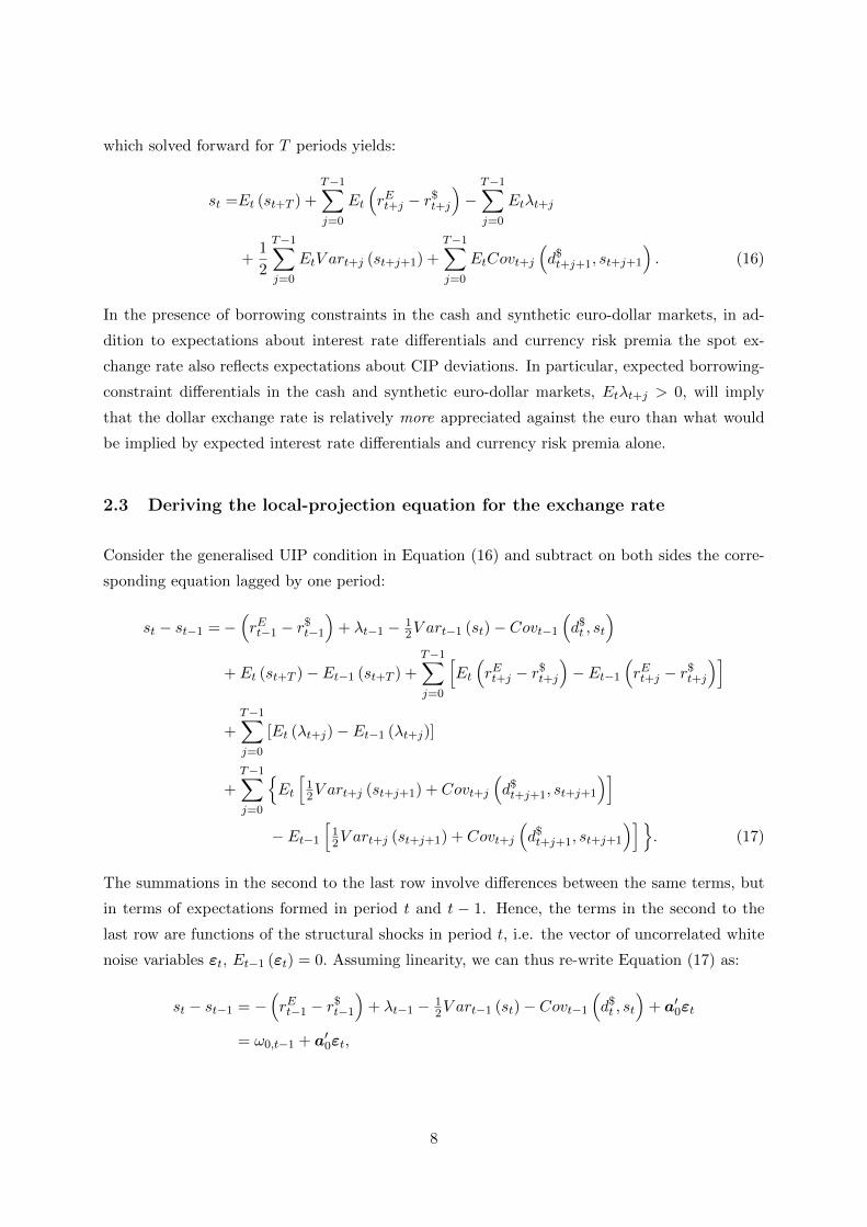
In the presence of borrowing constraints in the cash and synthetic euro-dollar markets, in ad-

dition to expectations about interest rate differentials and currency risk premia the spot ex-

change rate also reflects expectations about CIP deviations. In particular, expected borrowing-

constraint differentials in the cash and synthetic euro-dollar markets, Etλt+j > 0, will imply

that the dollar exchange rate is relatively more appreciated against the euro than what would

be implied by expected interest rate differentials and currency risk premia alone.

2.3 Deriving the local-projection equation for the exchange rate

Consider the generalised UIP condition in Equation (16) and subtract on both sides the corre-

sponding equation lagged by one period:

st − st−1 =−(rEt−1 − r$t−1

)+ λt−1 − 1

2V art−1 (st)− Covt−1(d$t , st

)+ Et (st+T )− Et−1 (st+T ) +

T−1∑j=0

[Et

(rEt+j − r$t+j

)− Et−1

(rEt+j − r$t+j

)]

+T−1∑j=0

[Et (λt+j)− Et−1 (λt+j)]

+T−1∑j=0

{Et

[12V art+j (st+j+1) + Covt+j

(d$t+j+1, st+j+1

)]− Et−1


(d$t+j+1, st+j+1

)]}. (17)

The summations in the second to the last row involve differences between the same terms, but

in terms of expectations formed in period t and t − 1. Hence, the terms in the second to the

last row are functions of the structural shocks in period t, i.e. the vector of uncorrelated white

noise variables εt, Et−1 (εt) = 0. Assuming linearity, we can thus re-write Equation (17) as:

st − st−1 = −(rEt−1 − r$t−1

)+ λt−1 − 1


)+ a′0εt

= ω0,t−1 + a′0εt,

8

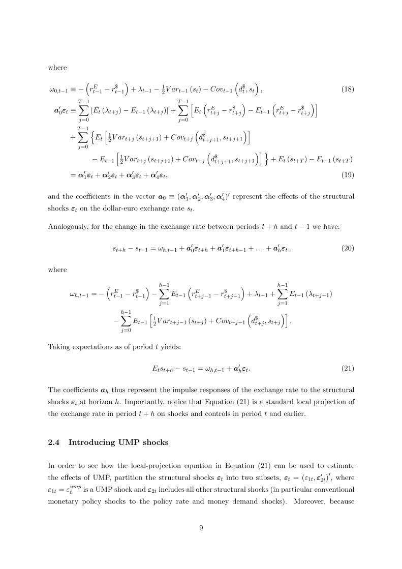
where

ω0,t−1 ≡ −(rEt−1 − r$t−1

)+ λt−1 − 1


), (18)

a′0εt ≡T−1∑j=0

[Et (λt+j)− Et−1 (λt+j)] +T−1∑j=0

[Et

(rEt+j − r$t+j

)− Et−1

(rEt+j − r$t+j

)]

+

T−1∑j=0

{Et


(d$t+j+1, st+j+1

)]− Et−1


(d$t+j+1, st+j+1

)]}+ Et (st+T )− Et−1 (st+T )

= α′1εt +α′2εt +α′3εt +α′4εt, (19)

and the coefficients in the vector a0 ≡ (α′1,α′2,α

′3,α

′4)′ represent the effects of the structural

shocks εt on the dollar-euro exchange rate st.

Analogously, for the change in the exchange rate between periods t+ h and t− 1 we have:

st+h − st−1 = ωh,t−1 + a′0εt+h + a′1εt+h−1 + . . .+ a′hεt, (20)

where

ωh,t−1 =−(rEt−1 − r$t−1

)−h−1∑j=1

Et−1

(rEt+j−1 − r$t+j−1

)+ λt−1 +

h−1∑j=1

Et−1 (λt+j−1)

−h−1∑j=0

Et−1

[12V art+j−1 (st+j) + Covt+j−1

(d$t+j , st+j

)].

Taking expectations as of period t yields:

Etst+h − st−1 = ωh,t−1 + a′hεt. (21)

The coefficients ah thus represent the impulse responses of the exchange rate to the structural

shocks εt at horizon h. Importantly, notice that Equation (21) is a standard local projection of

the exchange rate in period t+ h on shocks and controls in period t and earlier.

2.4 Introducing UMP shocks

In order to see how the local-projection equation in Equation (21) can be used to estimate

the effects of UMP, partition the structural shocks εt into two subsets, εt = (ε1t, ε′2t)′, where

ε1t = εumpt is a UMP shock and ε2t includes all other structural shocks (in particular conventional

monetary policy shocks to the policy rate and money demand shocks). Moreover, because

9

UMP measures are typically carried out over several periods, assume that εumpt includes a

contemporaneous component that reflects central bank asset purchases within the same period

denoted by ηt|t, as well as a component that is anticipated as of period t to be implemented in

period t+ 1 denoted by ηt+1|t:

εumpt = ηumpt|t + φ · ηumpt+1|t. (22)

In other words, while ηt|t captures unexpected UMP shocks that affect the balance sheet con-

temporaneously, ηt+1|t instead captures UMP shocks in t about measures that take place from

period t + 1 onwards. The intuition for including both a contemporaneous and an anticipated

future component in the UMP shock εumpt is that because the exchange rate is a forward-looking

asset price, it will not only respond to UMP measures announced and implemented in period t,

ηt|t, but also to those that are announced in t but that will only be — and are anticipated by

agents to be — implemented in period t+1, ηt+1|t. Moreover, notice that because the dollar-euro

exchange rate is a relative price, the term εumpt should be interpreted as a relative UMP shock,

i.e. UMP measures implemented by either the ECB or the Federal Reserve that affect the dif-

ference in central bank asset purchases. Partitioning the vector of impulse response coefficients

as a0 = (aump0 ,a′0,2)′, we can write the local-projection equation for the exchange rate as:

st − st−1 =ω0,t−1 + aump0

(ηumpt|t + φηumpt+1|t

)+ a′0,2ε2t. (23)

The impulse response of the exchange rate to the UMP shock εumpt is then given by the coefficients

aumph for horizons h = 0, . . . ,H.

Notice from Equation (20) that a′T−1εt = Et (st+T ) − Et−1 (st+T ), which is the revision in the

expectation of the exchange rate T periods in the future that occurs between periods t and t−1

as a result of shocks in period t. Thus, in case of a UMP shock, the estimate of aumpT−1 indicates

the importance of the signalling channel through effects of UMP measures on fundamentals and

monetary policy beyond period T . Finally, recalling the decomposition of the exchange rate in

Equation (16), notice that estimating the impulse responses of the fundamental determinants

allows us to quantify the transmission channels of the effects of UMP measures on the exchange

rate.

2.5 Proxying UMP shocks by changes in central banks’ balance sheets

Estimating the effects of UMP measures in the euro area and the US on the dollar-euro exchange

rate represented by {aumph }h=0,1,...,H in Equation (23) is complicated by the fact that the shocks

ηumpt|t and ηumpt+1|t are unobserved. However, we can proxy these relative UMP shocks by actual

changes in the relative size of central banks’ balance sheets that take place after UMP shocks.

10

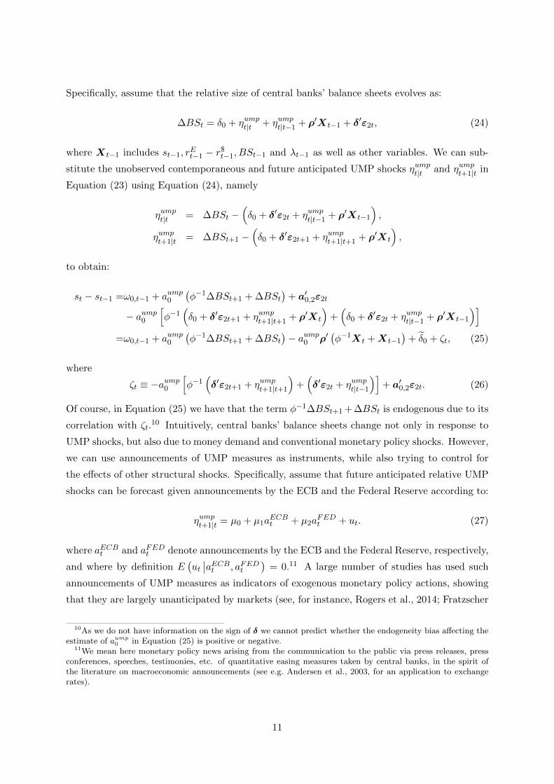
Specifically, assume that the relative size of central banks’ balance sheets evolves as:

∆BSt = δ0 + ηumpt|t + ηumpt|t−1 + ρ′Xt−1 + δ′ε2t, (24)

where Xt−1 includes st−1, rEt−1 − r$t−1, BSt−1 and λt−1 as well as other variables. We can sub-

stitute the unobserved contemporaneous and future anticipated UMP shocks ηumpt|t and ηumpt+1|t in

Equation (23) using Equation (24), namely

ηumpt|t = ∆BSt −(δ0 + δ′ε2t + ηumpt|t−1 + ρ′Xt−1

),

ηumpt+1|t = ∆BSt+1 −(δ0 + δ′ε2t+1 + ηumpt+1|t+1 + ρ′Xt

),

to obtain:

st − st−1 =ω0,t−1 + aump0

(φ−1∆BSt+1 + ∆BSt

)+ a′0,2ε2t

− aump0

[φ−1

(δ0 + δ′ε2t+1 + ηumpt+1|t+1 + ρ′Xt

)+(δ0 + δ′ε2t + ηumpt|t−1 + ρ′Xt−1

)]=ω0,t−1 + aump0

(φ−1∆BSt+1 + ∆BSt

)− aump0 ρ′

(φ−1Xt +Xt−1

)+ δ0 + ζt, (25)

where

ζt ≡ −aump0

[φ−1

(δ′ε2t+1 + ηumpt+1|t+1

)+(δ′ε2t + ηumpt|t−1

)]+ a′0,2ε2t. (26)

Of course, in Equation (25) we have that the term φ−1∆BSt+1 + ∆BSt is endogenous due to its

correlation with ζt.10 Intuitively, central banks’ balance sheets change not only in response to

UMP shocks, but also due to money demand and conventional monetary policy shocks. However,

we can use announcements of UMP measures as instruments, while also trying to control for

the effects of other structural shocks. Specifically, assume that future anticipated relative UMP

shocks can be forecast given announcements by the ECB and the Federal Reserve according to:

ηumpt+1|t = µ0 + µ1aECBt + µ2a

FEDt + ut. (27)

where aECBt and aFEDt denote announcements by the ECB and the Federal Reserve, respectively,

and where by definition E(ut∣∣aECBt , aFEDt

)= 0.11 A large number of studies has used such

announcements of UMP measures as indicators of exogenous monetary policy actions, showing

that they are largely unanticipated by markets (see, for instance, Rogers et al., 2014; Fratzscher

10As we do not have information on the sign of δ we cannot predict whether the endogeneity bias affecting theestimate of aump

0 in Equation (25) is positive or negative.11We mean here monetary policy news arising from the communication to the public via press releases, press

conferences, speeches, testimonies, etc. of quantitative easing measures taken by central banks, in the spirit ofthe literature on macroeconomic announcements (see e.g. Andersen et al., 2003, for an application to exchangerates).

11

et al., 2016, forthcoming). Then, consider the sum of Equation (24) over periods t and t+ 1:

∆BSt+1 + ∆BSt = ηumpt+1|t+1 + ηumpt+1|t + ηumpt|t + ηumpt|t−1

+2δ0 + ρ′(Xt +Xt−1) + δ′(ε2t+1 + ε2t),

and substitute ηumpt+1|t based on Equation (27) yielding:

∆BSt+1 + ∆BSt = µ0 + µ1aECBt + µ2a

FEDt + ρ′(Xt +Xt−1) + ξt, (28)

where

ξt ≡ ηumpt|t + ηumpt|t−1 + ηumpt+1|t+1 + δ′ε2t + δ′ε2t+1 + ut. (29)

Under the further identifying assumption that φ = 1, we can estimate aump0 in Equation (25) by

two-stage least squares, with Equation (28) as the first-stage regression in which announcements

of UMP measures aECBt and aFEDt by the ECB and the Federal Reserve represent instruments

for ∆BSt+1 + ∆BSt.

Three issues are worth pointing out. First, observe that if in Equation (23) we substituted

only ηumpt+1|t by ∆BSt+1, UMP announcements in period t might not be valid instruments for the

latter. Specifically, in this case ηumpt|t would appear in the error of Equation (25). Especially

when the frequency of the dataset is not very high — for example monthly, as in our baseline

specification — UMP announcements in period t might be correlated with ηumpt|t , because many

ECB announcements have taken place at the beginning of the month and purchases could

have started later in the same month.12 Second, a possible problem with our two-stage least

squares approach in Equations (25) and (28) is that UMP announcements may actually be

responses of the ECB and the Federal Reserve to other structural shocks ε2t. In this case,

UMP announcements in period t would not be valid instruments, as they would be correlated

with the error in Equation (25). As we explain in more detail in the next section, we address

this possibility by including a number of controls to capture the impact of the other structural

shocks ε2t, such as an index of macroeconomic news and the US VIX. Finally, since a specific

concern in the case of the ECB is that UMP measures may be deployed together with changes

in policy rates, in our empirical specification we also control for the differential between the

ECB main refinancing operations rate (MRO) and the Federal Funds target rate. Effectively,

this implies that we focus on balance sheet changes that are orthogonal to shocks affecting all

these contemporaneous variables.

12Having said that, as we have two instruments for the relative balance sheet — announcements by the ECBand the Federal Reserve — we can test for the validity of our instruments with a standard test of over-identifyingrestrictions in which we use only ∆Bt+1 instead of the sum ∆Bt+1 + ∆Bt. We do this in a robustness check inSection 5.

12

3 Empirical specification

We estimate Equations (25) and (28) by considering the ECB’s and the Federal Reserve’s balance

sheets as well as the nominal bilateral US dollar-euro exchange rate.13 We specify the relative

balance sheet size variable BSt as the difference between the nominal growth rates of the ECB’s

and the Federal Reserve’s balance sheets in their respective currencies (specifically the differential

in the respective log differences between periods t+ 1 and t− 1).

Since we are interested in the effect of UMP measures introduced in the wake of the global eco-

nomic and financial crisis and its aftermath, our sample period spans January 2009 to December

2016. In the baseline our analysis is carried out on data sampled at the monthly frequency.14 We

transform the data for financial variables available at higher frequencies to monthly observations

by calculating averages over daily or weekly data. The data on the dollar-euro exchange rate as

well as the size of the ECB’s and the Federal Reserve’s balance sheets are obtained from Haver

Analytics.

We specify the announcements aECBt and aFEDt as indicator variables which equal unity if the

ECB or the Federal Reserve announced in period t an asset purchase (see, for instance, Rogers

et al., 2014; Fratzscher et al., forthcoming, 2016). The dates of the announcements of UMP

measures by the ECB and the Federal Reserve are reported in Tables 1 and 2, respectively.15

The dates in question are assigned to their respective calendar month.16 As we are interested

in the impact of UMP measures in the form of central bank asset purchases, we only consider

announcements that can be assumed to have a tangible impact on the size of central banks’

balance sheets. For example, we do not include the announcements of the ECB’s intention to do

“whatever it takes to preserve the euro” in July 2012 and of the Outright Monetary Transactions

programme in September 2012, because these announcements did not result in asset purchases by

the time of writing. Furthermore, we do not include the ECB announcement of the Securities

Market Programme in May 2010, because the associated asset purchases were sterilised and

hence did not increase the ECB’s balance sheet.17 Tables 1 and 2 also include information on

the first principal component of the standardised one-day change of the German 2-year and 10-

year Bund and US Treasury yields on the day of the announcements. In all cases, the volatility

of changes in yields on the announcement days exceeds two standard deviations of the volatility

13In a future version of this paper we will also consider other major currency pairs.14In robustness checks we report results based on data sampled at the weekly frequency. Although weekly

sample would allow us a more accurate assignment of UMP announcements to the respective periods, we do notuse a weekly frequency in our baseline. The reason is that because of fluctuations in banks’ short-term liquidityneeds, the weekly data are significantly more noisy than the monthly data.

15The announcement dates of the UMP measures of the Federal Reserve are taken from Rogers et al. (2014).Those for the ECB are taken from the ECB’s website.

16The dummies also equal unity when there is more than one announcement in a given month, but this occursonly once in our dataset in the case of Federal Reserve announcements in October 2010.

17In robustness checks we added these three measures, however, and obtained similar results.

13

observed in our sample period, corroborating our assumption that these announcements were

surprise monetary policy actions.

In order to decompose the response of the exchange rate to changes in the relative size of the

central banks’ balance sheets as laid out in Equation (16), we also estimate the responses of

US and euro area interest rates, CIP deviations and risk premia by replacing the left-hand side

variable in Equation (25) accordingly. For interest rates, we consider three-month money market

rates as well as two and ten-year sovereign bond yields obtained from Haver Analytics; we use

German Bund yields as measures of euro area sovereign yields. We derive CIP deviations at the

three-months maturity or the dollar-euro exchange rate, λt, directly from Equation (13). We

take data on the three-months dollar-euro forward exchange rate from Bloomberg.

Finally, in the vector of controls Xt we include lagged announcements and lags of the three-

month and two-year interest rate differentials, the US dollar-euro exchange rate, the relative

balance sheet changes and CIP deviations, as well as lags and contemporaneous values of the

Citigroup Economic Surprise Indices for the US and the euro area obtained from Haver An-

alytics, the VIX, and the differential between the main ECB policy rate, the MRO, and the

Federal Reserve Federal Funds target. As explained above, by doing so we effectively control

for conventional monetary policy shocks in ε2t in Equation (26), which could contaminate the

estimation of the effects of UMP shocks.

4 Results

4.1 Predictive content of unconventional monetary policy announcements

Table 3 reports the estimates of our first-stage regression in Equation (28) for the relative balance

sheet variable BSt+1 −BSt−1.18 The estimates indicate that announcements of UMP measures

predict changes in central bank balance sheets. Especially ECB announcement dummies are

highly statistically significant and have a positive coefficient estimate. Specifically, following

an ECB UMP announcement, the ECB’s balance sheet expands by almost 4% relative to that

of the Federal Reserve. To put these numbers in perspective, recall from Figure 2 that this

amounts to an expansion of the ECB’s balance sheet relative to that of the Federal Reserve

somewhat more than 75 billion euros. Notice that this is roughly equivalent to the amount of

monthly asset purchases under the ECB’s Expanded Asset Purchase Programme launched in

2015. Conversely, UMP announcements by the Federal Reserve do not seem to be statistically

significant in accounting for changes in the relative balance sheet size.

18All standard errors in the tables are robust to heteroskedasticity and autocorrelation.

14

Finally, the results reported in Table 3 suggest that the estimated model passes the over-

identification (i.e. Hansen J) and the under-identification (Kleibergen-Paap) tests.19 In partic-

ular, the null of no correlation of the instruments with the relative balance sheet is rejected at

the 1% significance level. This means that we can have some confidence in relying on standard

asymptotic inference in reporting our results.

4.2 Dynamic effects of monetary policy supply shocks

We now turn to the dynamic responses of the relative size of central banks’ balance sheets, of the

nominal bilateral US dollar-euro exchange rate and of the variables involved in the decomposition

in Equation (16). All figures report asymptotic confidence bands at the 68% and 90% significance

levels, corrected to allow for heteroskedasticity and autocorrelation (dotted and dashed lines

respectively).

4.2.1 Balance sheet and policy rate responses

The left-hand side panel in Figure 3 shows the evolution of the relative balance sheet after a

UMP shock that increases the difference between the growth rates of the ECB’s and the Federal

Reserve’s balance sheets by one percentage point. Specifically, the impulse response in the figure

is obtained with our instrumental-variables local projections in which the dependent variable is

the (log of the level of the) relative balance sheet, for horizons h ≥ 2. Specifically, the ECB’s

balance sheet expands statistically significantly relative to that of the Federal Reserve for around

five months after the shock. The persistence of the relative balance sheet expansion is consistent

with the fact that UMP measures were typically not one-off instances of asset purchases or

liquidity injections, but implemented gradually or repeatedly over time.

It is important to make sure that the monetary policy shocks we measure by instrumenting the

relative balance sheet with UMP announcements really reflect unconventional monetary policy.

Specifically, it may be that UMP announcements are also followed by changes in conventional

monetary policy instruments. In this case, our estimates would not only reflect the effects of

UMP shocks, but also those from conventional monetary policy actions. As an external validity

test, we therefore estimate the responses of the ECB’s and Federal Reserve’s policy rates to our

presumed UMP shocks. We use the Federal Funds target rate for the Federal Reserve as well as

both the ECB’s main refinancing operations rate (MRO) and deposit facility rate (DFR).

The results are displayed in Figure 4. The differential between the ECB MRO rate and the

19The Hansen J-test of over-identification and the Kleibergen-Paap test of under-identification are tests ofwhether instruments are valid and meaningful, respectively.

15

Federal Funds target rate (left-hand side panel) barely responds.20 The point estimates are not

statistically significantly different from zero, except after 15 months when they turn negative.

The response of the differential between the ECB’s DFR and the Federal Funds target rate is

very similar to that of the MRO-Federal Funds target rate differential (right-hand side panel).

The point estimate is marginally statistically significant at the 68% confidence level between

three and four after the shock, but its economic magnitude of one basis point is minuscule.

Similarly to the MRO-Federal Funds target rate differential, the response turns negative and

statistically significant after 15 months. The finding of a lack of a economically (and, mostly,

statistically) significant negative impact of UMP shocks on the policy rate differential is all the

more noteworthy insofar as ECB policy rates were changed several times throughout our sample

period; for example, the ECB decreased the MRO rate from 2.5% in January 2009 to -0.05% in

March 2016, including four instances in which ECB UMP measures were announced alongside

conventional measures. Overall, these results suggest that the effects we estimate are related

to UMP shocks, and are not confounded with those from conventional monetary policy shocks.

In particular, as we show below, the negative interest rate differentials after 15 months do not

result in a corresponding response of the exchange rate or of money market interest rates.

4.2.2 Exchange rate response

The right-hand side panel in Figure 3 shows that the euro depreciates persistently in response

to a relative UMP shock reflected in an expansion of the ECB’s balance sheet relative to that of

the Federal Reserve by 1%. The response is statistically significant at the 90% (68%) level after

three (one) months and until the ten(twelve)-month horizon, over which the euro’s depreciation

bottoms at around 1.0%. Compared to the response of the relative balance sheet, the exchange

rate response is more persistent, returning to baseline only after around ten to twelve months;

importantly, notice that the exchange rate returns to baseline before the differential in policy

interest rates shown in Figure 4 turns negative. That the exchange rate response to a UMP shock

is mean-reverting, i.e. that Et (st+T ) −→ 0, implies that we can rule out that it is driven to a

large extent by expectations of exchange rate depreciation over horizons beyond twelve months,

and thus on account of expectations of future policy actions or changes in fundamentals.

4.2.3 Decomposition of the exchange rate response

We can now shed light on how UMP shocks are transmitted to the exchange rate through changes

in interest rate differentials, CIP deviations and currency risk premia.

20Recall that differential between the ECB MRO rate and the Federal Funds target rate is restricted not toreact to the expected increases in the relative balance sheet on impact due to the inclusion of this variable on theright-hand side of the local projections.

16

Interest rate differentials The top row in Figure 5 shows the response of the three-month

money market rate euro-dollar differential.21 The figure suggests that euro area money market

rates decline statistically significantly relative to those in the US in response to a relative UMP

shock in the euro area vis-a-vis the US. The three-month money market rate differential falls

statistically significantly at the 90% confidence level by up to around three basis points between

three and four months after the shock, when the exchange rate depreciates.22 At the 68% signif-

icance level, the fall in the short-term money market rate differential is statistically significant

after two months until at least 15 moths after the UMP shock.

The panels in the bottom row in Figure 5 present the responses of sovereign bond yield differ-

entials at the two and ten-year maturities. The relative UMP shock in the euro area vis-a-vis

the US has statistically significant effects on the sovereign bond yield differential only at the

shorter end of the yield curve, and only at the 68% level. In particular, in response to a 1% ex-

pansion in the ECB’s balance sheet relative to that of the Federal Reserve, the two-year interest

rate differential falls statistically significantly by almost three basis points after three months,

quickly reverting to baseline after six months.23 In contrast to two-year maturities, the relative

UMP shock in the euro area vis-a-vis the US does not affect the ten-year government bond yield

differential. The lack of a statistically significant response of ten-year sovereign bond yields may

seem counterintuitive against the backdrop of the APP program the ECB launched in January

2015. However, the estimated, relatively short-lived dynamics of the relative balance sheet de-

picted in Figure 3 seems consistent with the interpretation that our results mainly capture the

effects of prior ECB asset purchase programs, which were focused more on providing liquidity

to money markets. Thus, it is likely that the ECB asset purchase programs other than the APP

did not affect much long-term interest rates. This is consistent with results in Section 5, where

we show that excluding announcements related to the ECB APP program does not materially

change our results.

Overall, notice that our findings that (i) the exchange rate reverts back to baseline and that (ii)

longer-term yield differentials do not change imply that the signalling channel does not play a

major role for the transmission of UMP shocks.

CIP deviations The left-hand side panel in Figure 6 presents the response of the CIP de-

viation at the three-month maturity, defined such that a positive value amounts to a money

21Considering short-dated interest rates is important because default risk is less pronounced than for rates oflonger maturities, which would otherwise bias our estimates of the importance of the risk premia channel.

22Results available upon request show that the widening in short-term interest rate differentials is, in fact,driven almost exclusively by euro area money market rates.

23Analogous to the three-month money market differential, the widening in the two-year sovereign yield differ-ential is—as for money market rates—driven by a decline in euro area yields. These estimates are available uponrequest suggest that.

17

market euro rate, Ret , larger than the synthetic euro rate,StR

$t

Ft,t+1(or a larger synthetic dollar

rate,Ft,t+1Ret

Stthan its money market counterpart R$

t ). The three-month CIP deviation persis-

tently and statistically significantly falls in response to a relative UMP shock in the euro area

vis-a-vis the US, although the response is statistically significant at the 90% only after around 8

months. In particular, in response to a 1% expansion of the ECB’s balance sheet relative to that

of the Federal Reserve, the three-month CIP deviation falls by around three basis points. Given

that over our sample period CIP deviations have been persistently positive (money market euro

rates have been larger than synthetic euro rates), our results imply that a relative UMP shock

in the euro area vis-a-vis the US led to a narrowing in CIP deviations due to a reduction in

borrowing costs in euro money markets relative to those in synthetic funding markets.24 In order

to understand the economic implications of this result, recall the definition of the CIP deviation

from Section 2

λt ≡ 1− 1− λ$t1− λFt

.

Also recall that λ$t represents the shadow value of borrowing one additional euro in the synthetic

market (or one dollar in the cash market), while λFt represents the shadow value of borrowing

one additional euro in the cash market (or one dollar in the synthetic market). This equation

indicates that a fall in the CIP deviation can result only from a fall in λ$t relative to λFt . The

estimated effect on the CIP deviation is thus consistent with the notion that a relative UMP

shock in the euro area vis-a-vis the US lowers the cost of borrowing in euro money markets

relative to the cost of borrowing euro synthetically cum forward exchange rate in the dollar

money market. However, as we showed in Section 2.2, this reduction has to be associated with

a relative loosening of borrowing constraints in the latter relative to the former market.

According to Equation (14), changes in CIP deviations can be further decomposed into move-

ments in interest rate differentials and forward-spot exchange rate differentials (forward dis-

count), namely

λt = ret − r$t + ft,t+1 − st. (30)

We have already shown that the money market rate differential falls by around three basis points

in response to a relative UMP shock in the euro area vis-a-vis the US (see Figure 5). Analogously,

the right-hand side panel in Figure 6 shows the response of three-month dollar-euro forward-spot

differential. The latter peaks at around one basis point after three months. This is less than what

would be required to keep CIP deviations constant. The response of the CIP deviation at the

three-month maturity is thus mainly driven by the more subdued adjustment in the dollar-euro

forward-spot response, relative to the response in the money market rate differential. Recall that

according to the decomposition of the exchange rate in Equation (16), a fall in CIP deviations

24Notice that the market convention is to denote CIP deviations — the cross-currency basis swap — with theopposite sign compared to our notation.

18

strengthens the euro relative to the dollar. As we show below, the contribution of the response

of CIP deviations is thus to appreciate the euro relative to the US dollar, overall resulting in

a more subdued depreciation than what would be warranted by the decline in the interest rate

differential and risk premia.

Decomposing the exchange rate response Based on the estimated responses of the inter-

est rate differentials, the expected future exchange rate and the CIP deviations and Equation

(16)

st − Et (st+T ) =

{T−1∑j=0

Et

(ret+j − r$t+j

)−T−1∑j=0

Et (λt+j)

+T−1∑j=0

Et

[1

2V art+j (st+j+1) + Covt+j

(d$t+j+1, st+j+1

)]},

we can determine which transmission channel contributes by how much at different horizons to

the overall exchange rate response. Figure 7 presents the cumulated responses of the fundamental

determinants of the exchange rate shown on the right-hand side of Equation (16) and based on

the estimates shown in Figures 3 to 6; the implied contribution of the currency risk premia is

obtained as the residual given the estimated responses of the exchange rate, the three-month

money market differential and the CIP deviations. Specifically, the decomposition shows that on

impact, falling current and expected future interest rate differentials and risk premia depreciate

the euro relative to the US dollar; however, the expected appreciation at the 15 month horizon

and the fall in CIP deviations almost completely offsets this. Both the depreciating effect of the

decline in interest rate differentials, and the countervailing CIP deviations fade over time due

to their mean reversion, while the contribution of the expected end-of period appreciation is

constant over all periods. Therefore, the bulk of the estimated depreciation of the euro against

the US dollar must be driven by a fall in dollar-euro currency risk premia. Recall from Section

2.1 that a smaller risk premium implies that the euro is now expected to be weaker relative

to the dollar when the marginal value of a US investor’s US dollar wealth is higher (St+1 is

expected to be less positively — or even negatively — related to D$t+1 in Equation (7)).

4.3 Impact of unconventional monetary policy shocks on the real economy

and stock markets

The responses of the long-term yield differentials discussed above raises the question of whether

the UMP shock might not affect much other financial markets and economic activity. Looking

first at US and euro area stock markets, the impulse responses of the Eurostoxx 300 and the

19

S&P500 shown in Figure 8 suggest that both indexes increase, especially in the euro area.

However, only the rise in the Eurostoxx 300 by 1% after six to eight months is statistically

significant at the 90% level.

Conversely, when we look at the UMP effects on economic activity in the euro area and the US, we

find little evidence of strong effects. While the euro-dollar nominal depreciation translates into

a real depreciation, though smaller and a bit less precisely estimated, the responses of industrial

production growth and HICP inflation in the euro area are small and not statistically significant,

as shown in Figure 10. However, industrial production and especially inflation decrease in the

US, the latter briefly even at the 90% level after four to five months, as shown in Figure 11.

Our evidence thus suggests that the impact of the relative UMP shock is mostly confined to

exchange rate and money markets.

5 Robustness

We now explore the sensitivity of our baseline results to the following: (i) substituting only the

anticipated relative UMP shock in Equation (23); (ii) relying on OLS estimates with no instru-

ments; (iii) using higher-frequency, weekly data; (iv) dropping the ECB UMP announcements

related to the APP program from the set of indicator variables.

5.1 Purely anticipated relative balance sheet shock

Our first sensitivity check is to explore how our results are affected if we only substitute the

anticipated shock ηMSt+1|t by ∆BSt+1. The local-projection equation is then given by:

st − st−1 =ω0,t−1 + aump0 φ−1∆BSt+1 + a′0,2ε2t

− aump0 φ−1(δ0 + δ′ε2t+1 + ηumpt+1|t+1 + ρ′Xt

)+ aump0 ηMS

t|t

=ω0,t−1 + aump0 φ−1∆BSt+1 − aump0 ρ′φ−1Xt + δ0

+ a′0,2ε2t − aump0 φ−1

(δ′ε2t+1 + ηumpt+1|t+1

)+ aump0 ηMS

t|t , (31)

where we include the same contemporaneous and lagged controls as in the baseline specification.

Observe that now the contemporaneous balance sheet shock ηt|t is in the error term, which

amounts to assuming that announcements are not correlated with it. Evidence against this

assumption can be provided by the standard Hansen J-test of instrument validity. However, as

shown by the estimation results reported in Table 4 for the first stage regression, this specification

20

also passes the tests of instrument validity and relevance.25 As shown in Figure 12, the impulse

responses of the relative balance sheet, the dollar-euro exchange rate, of the differential between

the ECB’s MRO rate and the Federal Funds target rate, and the three-month rate differential

are broadly consistent with those from our baseline results. Moreover, the relative balance

sheet does not increase statistically significant on impact. These results thus suggest that the

UMP announcements we consider mainly convey information about future central bank asset

purchases beyond period t.

5.2 OLS estimates

Given the endogeneity of central banks’ balance sheets, the error term in Equation (26) is likely

to be correlated with the variable of interest ∆BSt+1 + ∆BSt in our local-projection equation.

As we do not have information on the sign of δ in Equation (24), we cannot predict whether the

endogeneity bias affecting the estimate of aump0 in Equation (25) is positive or negative. However,

it is still useful to assess how severe the endogeneity bias ultimately is. To do so, we can estimate

Equation (26) by OLS. Figure 13 displays the results, suggesting that the endogeneity bias is

quantitatively significant. Specifically, according to the OLS estimates, the euro depreciates only

by up to 0.4% against the US dollar, substantially less than the 1% in the baseline in Figure

3. Moreover, according to the OLS estimates the relative balance sheet increases statistically

significantly even on impact, which is consistent with endogeneity bias due to the correlation

between the difference in the relative balance sheet griwth rates ∆BSt+1 + ∆BSt and the error

term ζt in Equation (26).

5.3 Weekly data

Our baseline estimates are based on monthly data, which we obtain from averaging weekly

data. We consider the monthly frequency because fluctuations in banks’ short-term liquidity

needs cause substantial noise in weekly data, which inflates the estimation error. In principle,

however, exploring the weekly frequency has the advantage that it allows us to assign more

accurately the UMP announcements to the respective periods, and thereby improve the power

of our instruments. Figure 14 displays the results from our estimations when they are carried out

using weekly data.26 As expected, the results are less precisely estimated, but, more importantly,

our baseline findings are largely confirmed. A relative UMP shock in the euro area vis-a-vis the

25The main difference with the benchmark specification is that Fed announcements now have — implausibly —a statistically significant and positive coefficient, implying that they are associated with an increase in the ECB’sbalance sheet relative to that of the Federal Reserve.

26Similarly with the first robustness exercise, we proxy the UMP shocks with relative balance sheet growth inthe four weeks after that of the announcement.

21

US gradually and statistically significantly increases the relative balance sheet over around 20

weeks, resulting in a delayed euro depreciation lasting for a similar period, and in a decline of

the three-month money market rate differential. Quantitatively, the maximum depreciation of

1% and fall in the interest rate differential by four-basis points are quite similar to our baseline

results based on monthly data.

5.4 Excluding APP announcements from the set of instruments

The announcements of the UMP measures of the ECB and the Federal Reserve we consider

as instruments are coded as binary dummy variables in our baseline specification. This is

potentially an issue as we are treating potentially different UMP measures as the same. This

concern is relevant for the ECB, whose APP program, geared towards asset purchases, was

different from prior measures mainly targeting bank liquidity demand. In this subsection we

thus investigate whether our results are sensitive to excluding announcements about the ECB

APP program. The results are displayed in Figure 15, and are very similar to our baseline

findings. This is consistent with the view that in our sample we are mainly capturing the effects

of the ECB and Feder Reserve UMP measures prior to 2015.

6 Concluding remarks

[To be written.]

References

Altavilla, C., Carboni, G., Motto, R., 2015. Asset purchases and financial markets: evidence

from the Euro Area. mimeo.

Andersen, T. G., Bollerslev, T., Diebold, F. X., Vega, C., March 2003. Micro Effects of Macro

Announcements: Real-Time Price Discovery in Foreign Exchange. American Economic Review

93 (1), 38–62.

Borio, C., McCauley, R., McGuire, P., Sushko, V., September 2016. Covered Interest Parity

Lost: Understanding the Cross-currency Basis. BIS Quarterly Review.

Du, W., Tepper, A., Verdelhan, A., 2017. Deviations from Covered Interest Rate Parity. NBER

Working Papers 23170.

22

Fratzscher, M., Lo Duca, M., Straub, R., 2016. ECB Unconventional Monetary Policy: Market

Impact and International Spillovers. IMF Economic Review 64 (1), 36–74.

Fratzscher, M., Lo Duca, M., Straub, R., forthcoming. On the International Spillovers of US

Quantitative Easing. Economic Journal.

Gambacorta, L., Hofmann, B., Peersman, G., 2014. The Effectiveness of Unconventional Mon-

etary Policy at the Zero Lower Bound: A Cross-country Analysis. Journal of Money, Credit

and Banking 46 (4), 615–642.

Garcia-de Andoain, C., Heider, F., Hoerova, M., Manganelli, S., 2016. Lending-of-last-resort

is as Lending-of-last-resort Does: Central Bank Liquidity Provision and Interbank Market

Functioning in the Euro Area. Journal of Financial Intermediation 28 (C), 32–47.

Georgiadis, G., Grab, J., 2016. Global Financial Market Impact of the Announcement of the

ECB’s Asset Purchase Programme. Journal of Financial Stability 26 (C), 257–265.

Glick, R., Leduc, S., 2015. Unconventional Monetary Policy and the Dollar: Conventional Signs,

Unconventional Magnitudes. Federal Reserve Bank of San Francisco Working Paper 2015-18.

Jorda, O., 2005. Estimation and Inference of Impulse Responses by Local Projections. American

Economic Review 95 (1), 161–182.

Kouri, P., 1976. The Exchange Rate and the Balance of Payments in the Short Run and in the

Long Run: A Monetary Approach. Scandinavian Journal of Economics 78, 280–304.

Krishnamurthy, A., Nagel, S., Vissing-Jorgensen, A., 2014. ECB Policies involving Government

Bond Purchases: Impact and Channels. mimeo.

Krishnamurthy, A., Vissing-Jorgensen, A., 2011. The Effects of Quantitative Easing on Interest

Rates: Channels and Implications for Policy. Brookings Papers on Economic Activity 43 (2

(Fall)), 215–287.

Lucas, R., 1978. Asset Prices in an Exchange Economy. Econometrica 46 (6), 1429–45.

Mertens, K., Ravn, M., 2011. Understanding the Aggregate Effects of Anticipated and Unantic-

ipated Tax Policy Shocks. Review of Economic Dynamics 14 (1), 27–54.

Neely, C., 2015. Unconventional Monetary Policy Had Large International Effects. Journal of

Banking & Finance 52 (C), 101–111.

Rogers, J., Scotti, C., Wright, J. H., October 2014. Evaluating Asset-market Effects of Uncon-

ventional Monetary Policy: A Multi-country Review. Economic Policy 29 (80), 749–799.

23

Weale, M., Wieladek, T., 2016. What Are the Macroeconomic Effects of Asset Purchases? Jour-

nal of Monetary Economics 79 (C), 81–93.

Woodford, M., 2012. Methods of Policy Accommodation at the Interest-rate Lower Bound.

Proceedings - Economic Policy Symposium - Jackson Hole, 185–288.

24

A Can CIP deviations arise due to counterparty risk?

Under the maintained assumption that REt is risk free, a simple way of thinking of counterparty

risk in the forward exchange rate market is the following. Rather than at the contracted, known

exchange rate Ft,t+1, the conversion into dollars of the one-period euro payoff REt may be risky

if there is a probability that it has to take place on the spot market at the uncertain (risky)

exchange rate St+1 because the counterparty cannot deliver dollars anymore. Assuming the

(conditional) probability of the latter event is πt, we have that no-arbitrage under no borrowing

constraints implies the following:27

(1− πt)Et(D$t+1

)Ft,t+1 + πtEt

(St+1D$

t+1

)St

Rte = Et

(D$t+1

)R$t = 1

Ft,t+1Rte

St> R$

t <=> (Et (St+1)− Ft,t+1)− Covt(D$t+1, St+1

)R$t > 0.

Thus a sufficient condition for positive CIP deviations (Ft,t+1Rte

St> R$

t ) is that the expression[(Et (St+1)− Ft,t+1)− Covt

(D$t+1, St+1

)R$t

]is different from zero. However, it is possible to

show that this expression is always zero, as it corresponds to the expected forward premium

(see e.g. Engel 1999). For our investor, it should be the case that the one period risk-adjusted

expected return of investing in the dollar euro forward market or in the dollar euro spot market

should be the same, namely

πtEt

(St+1D$

t+1

)+ (1− πt)Et

(D$t+1

)Ft,t+1

StRte =

Et

(D$t+1St+1

)St

Rte

(1− πt)Et

(D$t+1

)Ft,t+1

StRte = (1− πt)

Et

(D$t+1St+1

)St

Rte.

Ft,t+1 = Et (St+1)−Covt

(D$t+1, St+1

)Et

(D$t+1

) (A.1)

Notably, these returns are equalized also if they are subject to the same borrowing constraints

and transaction costs. But then it is immediate that deviations from CIP cannot arise from

counterparty forward market risks that are perfectly correlated with future spot market risks.The

27

Et

(D$

t+1

)Ft,t+1 + πt

[Et

(D$

t+1

)(Et (St+1)− Ft,t+1)− Covt

(D$

t+1, St+1

)]St

Rte = Et

(D$

t+1

)R$

t

Ft,t+1RteSt

1 + πt

(Et (St+1)− Ft,t+1)−R$tCovt

(D$

t+1, Ft,t+1

)Ft,t+1

= R$t

25

same relation for the “European” investor would read

Ft,t+1 =

[Et (1/St+1)−

Covt (Dt+1e, 1/St+1)

Et (Dt+1e)

]−1.

26

B Tables

Table 1: ECB announcements of unconventional monetary policy measures

Date Event Bond marketresponse

07/05/2009 12-month SLTROs and other measures 8.3704/08/2011 SLTROs and other measures -7.2706/10/2011 12/13-month SLTROs 4.1108/12/2011 36-month VLTROs and other measures -3.4305/06/2014 Targeted longer term refinancing operations (TLTROs) -4.2604/09/2014 Announcement of ABSPP and CBPP3 1.0202/10/2014 Details for the ABSPP and CBPP3 -.4022/01/2015 Expanded Asset purchase programme (APP) -7.1905/03/2015 Implementation details of APP -2.9703/09/2015 Increase of PSPP’s issue share limit -5.8110/03/2016 CSPP announcement 3.8521/04/2016 CSPP starting date announcement and details 2.4902/06/2016 CSPP Implementation details -2.2808/12/2016 Extension of APP -2.02

Note: The bond market response is based on the first principal component of the standardized one-day changeof the German 2-year and 10-year bund yields on the day of the announcements. Values are standardized withmean equal to zero and standard deviation equal to unity.

Table 2: Fed announcements of unconventional monetary policy measures

Date Event Bond marketresponse

28/01/2009 Fed stands ready to expand QE and buy Treasuries 2.4018/03/2009 LSAPs expanded -15.3227/08/2010 Bernanke suggest role for additional QE 3.9312/10/2010 FOMC members ‘sense’ ‘additional accommodation appropri-

ate’1.09

15/10/2010 Bernanke reiterates Fed stands ready to further ease policy 1.2403/11/2010 QE2 announced: Fed will purchase $600 bn in Treasuries -.1121/09/2011 Maturity Extension Program announced .1420/06/2012 Maturity Extension Program extended .7322/08/2012 FOMC members ‘judge additional accommodation likely war-

ranted’-2.68

13/09/2012 QE3 announced: Fed will purchase $40 bn of MBS per month -1.1712/12/2012 QE3 expanded 1.07

Note: The bond market response is based on the first principal component of the standardized one-day changeof the US 2-year and 10-year Treasury yields on the day of the announcements. Values are standardized withmean equal to zero and standard deviation equal to unity.

27

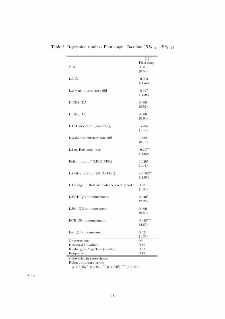
Table 3: Regression results - First stage—Baseline (BSt+1 −BSt−1)

(1)First stage

VIX 0.001(0.55)

L.VIX -0.003+

(-1.52)

L.2-year interest rate diff -6.027(-1.26)

D.CESI EA 0.000(0.57)

D.CESI US 0.000(0.60)

L.CIP deviation (3-months) 17.854(1.40)

L.3-months interest rate diff 1.832(0.16)

L.Log Exchange rate -0.247+

(-1.60)

Policy rate diff (MRO-FFR) 10.265(1.11)

L.Policy rate diff (MRO-FFR) -16.462∗∗

(-2.05)

L.Change in Relative balance sheet growth 0.221(1.03)

L.ECB QE announcement 0.040∗∗

(2.24)

L.Fed QE announcement 0.009(0.53)

ECB QE announcement 0.038∗∗∗

(2.65)

Fed QE announcement 0.021(1.35)

Observations 95Hansen-J (p-value) 0.42Kleibergen-Paap-Test (p-value) 0.01R-squared 0.49

t statistics in parenthesesRobust standard errors+ p < 0.15, ∗ p < 0.1, ∗∗ p < 0.05, ∗∗∗ p < 0.01

Notes:

28

Table 4: Regression results - First stage—Robustness 2 (BSt+1 −BSt)

(1)First stage

VIX 0.001(0.42)

L.VIX -0.001(-0.63)

L.2-year interest rate diff -1.526(-0.50)

D.CESI EA 0.000(0.73)

D.CESI US 0.000(0.71)

L.CIP deviation (3-months) 10.684(1.22)

L.3-months interest rate diff -1.464(-0.18)

L.Log Exchange rate -0.128(-1.31)

Policy rate diff (MRO-FFR) 7.336(1.27)

L.Policy rate diff (MRO-FFR) -11.238∗∗

(-2.14)

L.Change in Relative balance sheet growth 0.014(0.12)

L.ECB QE announcement 0.012(0.90)

L.Fed QE announcement -0.014(-1.06)

ECB QE announcement 0.029∗∗∗

(3.17)

Fed QE announcement 0.018∗

(1.74)

Observations 95Hansen-J (p-value) 0.40Kleibergen-Paap-Test (p-value) 0.01R-squared 0.35

t statistics in parenthesesRobust standard errors+ p < 0.15, ∗ p < 0.1, ∗∗ p < 0.05, ∗∗∗ p < 0.01

Notes:

29

C Figures

Figure 1: Absolute balance sheet movements and UMP announcements

1500

2000

2500

3000

3500

EU

R b

illio

n

2009m1 2010m1 2011m1 2012m1 2013m1 2014m1 2015m1 2016m1date

ECB balance sheet ECB QE Announcements

1500

2000

2500

3000

3500

4000

US

D b

illio

n

2009m1 2010m1 2011m1 2012m1 2013m1 2014m1 2015m1 2016m1date

US Fed balance sheet Fed UMP Announcements

Notes: The figure shows the evolution of the ECB’s (left-hand side panel) and the Federal Reserve’s (right-handside panel) balance sheets. In both panels, the vertical lines indicate the dates of UMP announcements by therespective central bank.

Figure 2: Relative balance sheet movements and the EUR/USD exchange rate

−.4

−.3

−.2

−.1

0lo

g E

UR

/US

D e

xcha

nge

rate

−.1

−.0

50

.05

.1lo

g−ch

ange

in r

elat

ive

bala

nce

shee

t

2009m1 2010m1 2011m1 2012m1 2013m1 2014m1 2015m1 2016m1date

Relative balance sheet (ECB/FED) EUR/USD

Notes: The figure shows the evolution of the logarithm of the nominal euro-US dollar exchange rate (dashed redline) and the difference between the growth rates of the ECB’s and the Federal Reserve’s balance sheets (solid blueline).

30

Figure 3: Relative balance sheet and exchange rate responses

Relative balance sheet US dollar-euro exchange rate(deviation from baseline in %) (US dollar per euro, deviation from baseline in %)

−4

−2

02

0 5 10 15month

−2

−1.

5−

1−

.50

.50 5 10 15

month

Notes: The panels show the responses to a UMP shock that increases the difference between the growth rates ofthe ECB’s and the Federal Reserve’s balance sheets by one percentage point.

Figure 4: Policy rate differential

MRO - Fed Funds rate DFR - Fed Funds rate(deviation from baseline in %-age points) (deviation from baseline in %-age points)

−.0

4−

.02

0.0

2

0 5 10 15month

−.0

4−

.02

0.0

2

0 5 10 15month

Notes: The panels show the responses to a relative UMP shock that increases the difference between the growthrates of the ECB’s and the Federal Reserve’s balance sheets by one percentage point.

31

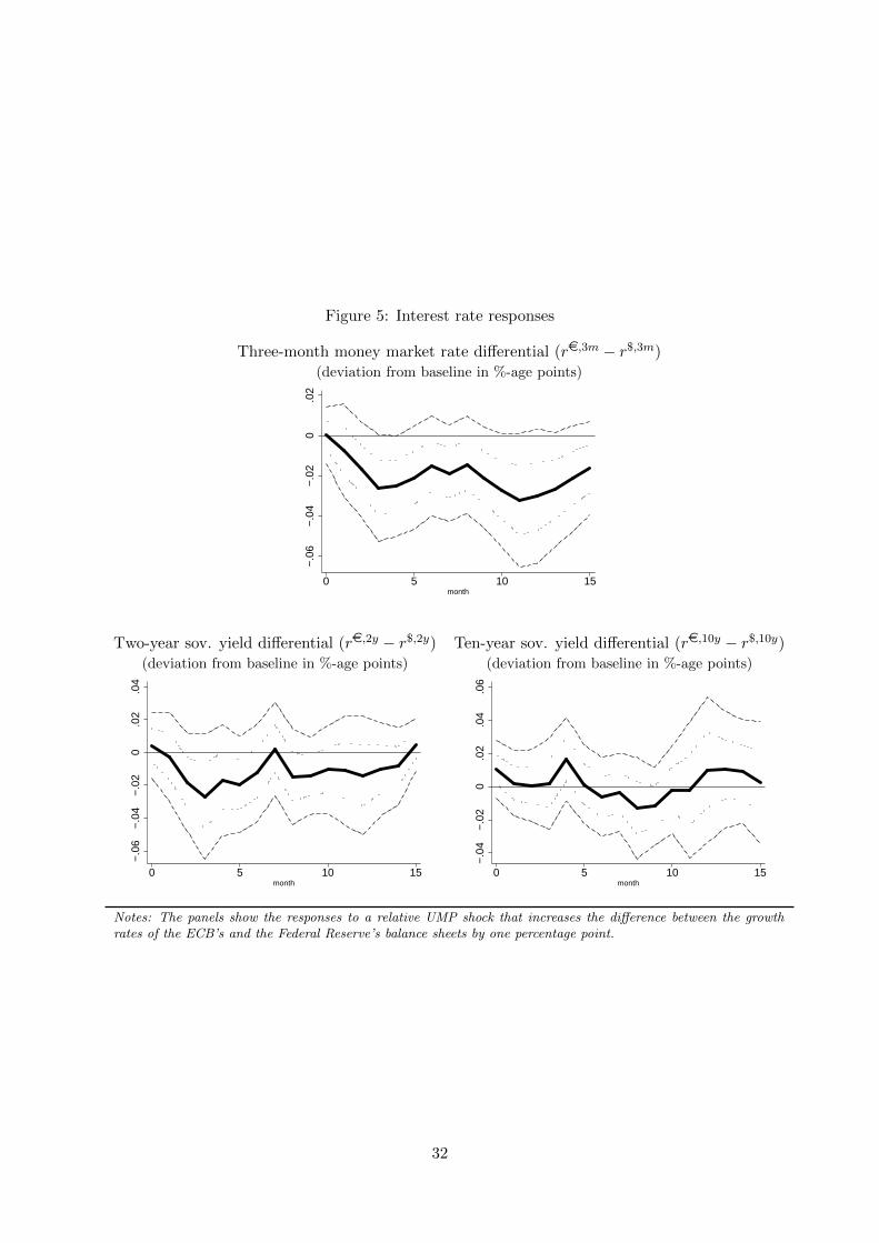
Figure 5: Interest rate responses

Three-month money market rate differential (re,3m − r$,3m)(deviation from baseline in %-age points)

−.0

6−

.04

−.0

20

.02

0 5 10 15month

Two-year sov. yield differential (re,2y − r$,2y) Ten-year sov. yield differential (re,10y − r$,10y)(deviation from baseline in %-age points) (deviation from baseline in %-age points)

−.0

6−

.04

−.0

20

.02

.04

0 5 10 15month

−.0

4−

.02

0.0

2.0

4.0

6

0 5 10 15month


32

Figure 6: Three-month CIP deviation and forward-spot rate differential

CIP deviation (λt = f3mt,t+1 − st + re,3mt − r$,3mt ) Forward-spot rate diff. (f3mt,t+1 − st)(deviation from baseline in %-age points) (deviation from baseline in %)

−.0

6−

.04

−.0

20

.02

0 5 10 15month

−.0

10

.01

.02

0 5 10 15month


Figure 7: Decomposition of exchange rate response to UMP shocks

−1.

5−

1−

.50

.5

0 1 2 3 4 5 6 7 8 9 10 11 12 13 14 15

3m−MM−diff 3m−CIP−deviationRisk premium Expected exchange rate in H

Notes: The figure shows the decomposition of the exchange rate effect of a relative UMP shock that increases thedifference between the growth rates of the ECB’s and the Federal Reserve’s balance sheets by one percentage pointinto the transmission channels according to Equation (16).

33

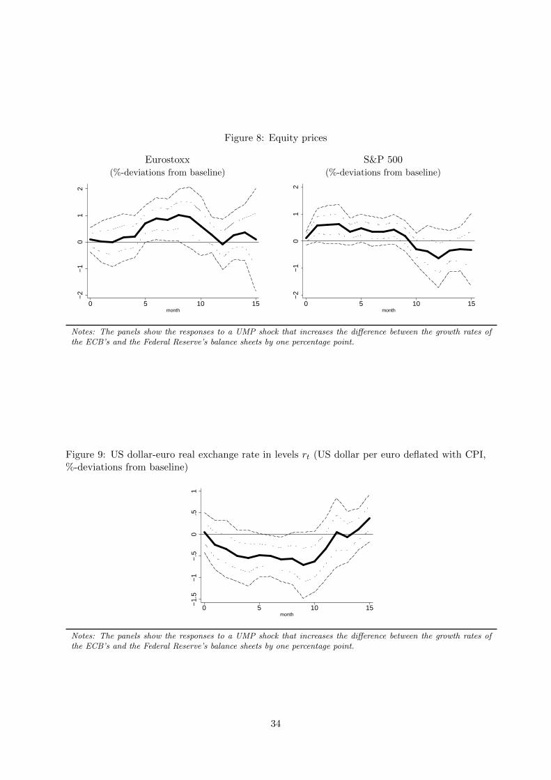
Figure 8: Equity prices

Eurostoxx S&P 500(%-deviations from baseline) (%-deviations from baseline)

−2

−1

01

2

0 5 10 15month

−2

−1

01

20 5 10 15

month


Figure 9: US dollar-euro real exchange rate in levels rt (US dollar per euro deflated with CPI,%-deviations from baseline)

−1.

5−

1−

.50

.51

0 5 10 15month


34

Figure 10: Euro area real variables

Industrial production HICP inflation(%-deviations from baseline) (%-points deviations from baseline)

−.4

−.2

0.2

.4

0 5 10 15month

−.1

5−

.1−

.05

0.0

5.1

0 5 10 15month


Figure 11: US real variables

Industrial production HICP inflation(%-deviations from baseline) (%-points deviations from baseline)

−.3

−.2

−.1

0.1

.2

0 5 10 15month

−.4

−.2

0.2

0 5 10 15month


35

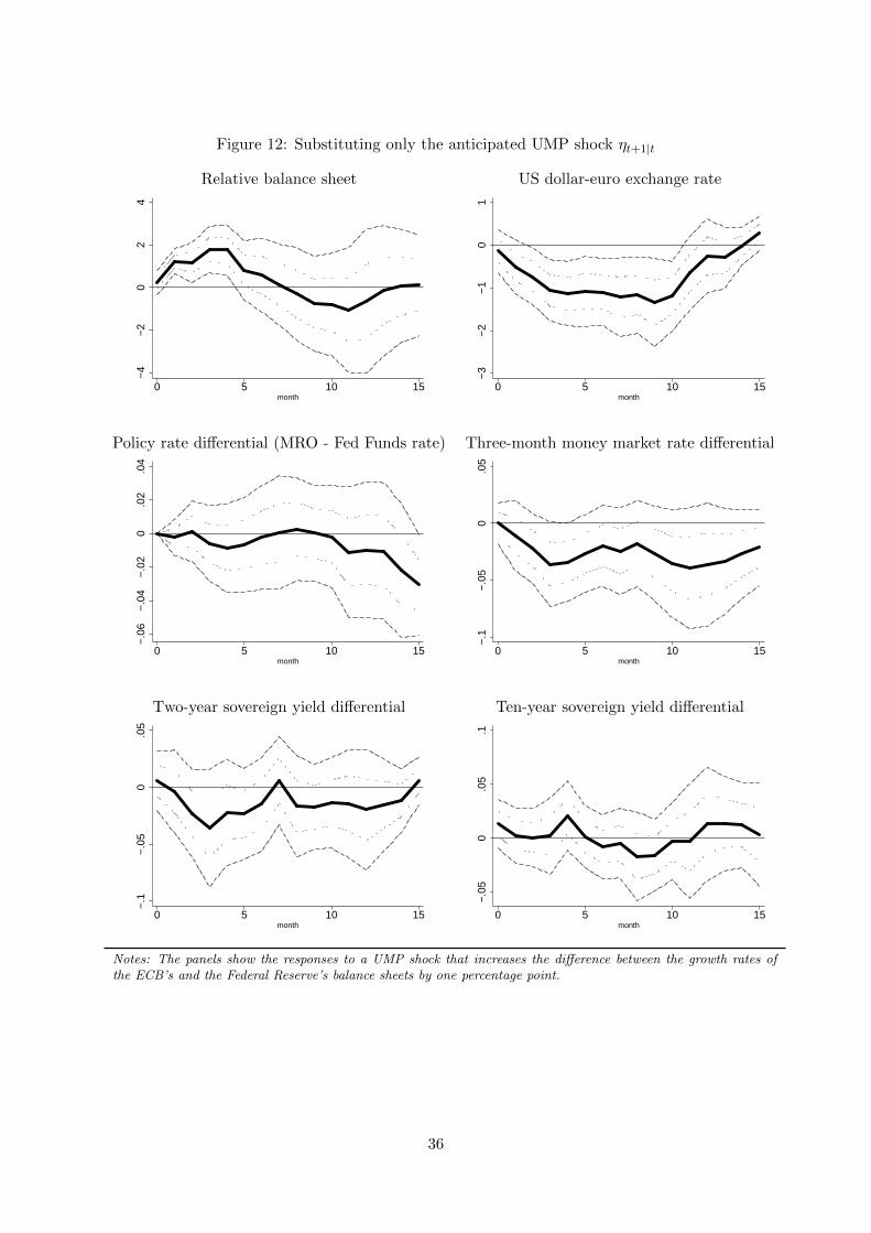
Figure 12: Substituting only the anticipated UMP shock ηt+1|t

Relative balance sheet US dollar-euro exchange rate

−4

−2

02

4

0 5 10 15month

−3

−2

−1

01

0 5 10 15month

Policy rate differential (MRO - Fed Funds rate) Three-month money market rate differential

−.0

6−

.04

−.0

20

.02

.04

0 5 10 15month

−.1

−.0

50

.05

0 5 10 15month

Two-year sovereign yield differential Ten-year sovereign yield differential

−.1

−.0

50

.05

0 5 10 15month

−.0

50

.05

.1

0 5 10 15month


36

Figure 13: OLS results


−.5

0.5

11.

5

0 5 10 15month

−.4

−.2

0.2

.4

0 5 10 15month


−.0

3−

.02

−.0

10

.01

.02

0 5 10 15month

−.0

4−

.02

0.0

2

0 5 10 15month


−.0

4−

.02

0.0

2.0

4

0 5 10 15month

−.0

2−

.01

0.0

1.0

2

0 5 10 15month


37

Figure 14: Weekly frequency


−4

−2

02

4

0 10 20 30 40 50week

−3

−2

−1

01

0 10 20 30 40 50week


−.1

−.0

50

.05

.1

0 10 20 30 40 50week

−.1

−.0

50

.05

.1

0 10 20 30 40 50week


−.1

−.0

50

.05

.1

0 10 20 30 40 50week

−.1

−.0

50

.05

.1.1

5

0 10 20 30 40 50week


38

Figure 15: Excluding APP announcements


−4

−2

02

0 5 10 15month

−2

−1.

5−

1−

.50

.5

0 5 10 15month


−.0

4−

.02

0.0

2

0 5 10 15month

−.0

6−

.04

−.0

20

.02

0 5 10 15month


−.0

6−

.04

−.0

20

.02

.04

0 5 10 15month

−.0

4−

.02

0.0

2.0

4.0

6

0 5 10 15month


39

Does a Big Bazooka Matter? Central Bank Balance-Sheet ...cepr.org/sites/default/files/1884_DEDOLA -...

Documents

Transcript of Does a Big Bazooka Matter? Central Bank Balance-Sheet ...cepr.org/sites/default/files/1884_DEDOLA -...