DOCUMENTS DE TREBALL

DE LA FACULTAT DE CIÈNCIES

ECONÒMIQUES I EMPRESARIALS

Col·lecció d’Economia

New Estimates of Regional GDP in Spain, 1860-1930*

Julio Martínez Galarraga

Universitat de Barcelona

Adreça correspondència: Departament d’Història i Institucions Econòmiques Facultat de Ciències Econòmiques i Empresarials Universitat de Barcelona Av. Diagonal 690 08034 Barcelona (Spain) e-mail: julio.martinez@ub.edu ∗ I would like to thank Daniel A. Tirado and Kerstin Enflo for their suggestions and help. Also the participants at the ‘Grup de Recerca en Globalització, Desigualtat Econòmica i Polítiques Públiques” work session in November 2006 for their insightful comments, especially Marc Badia-Miró, Sergio Espuelas, Jordi Guilera, Alfonso Herranz, Jordi Pons, Marc Prat and Ramon Ramon.

Abstract:

This paper presents a new regional database on GDP in Spain for the years 1860, 1900, 1914

and 1930. Following Geary and Stark (2002), country level GDP estimates are allocated across

Spanish provinces. The results are then compared with previous estimates. Further, this new

evidence is used to analyze the evolution of regional inequality and convergence in the long

run. According to the distribution dynamics approach suggested by Quah (1993, 1996)

persistence appears as a main feature in the regional distribution of output. Therefore, in the

long run no evidence of regional convergence in the Spanish economy is found.

JEL Classification: N93, N94, O18, O47, E01

Keywords: regional GDP, economic history, economic growth, convergence, distribution

dynamics.

Resumen:

En este trabajo se presenta una estimación del PIB provincial y regional para los años 1860,

1900, 1914 y 1930. La metodología propuesta por Geary y Stark (2002), permite distribuir

el PIB per capita español entre las provincias españolas. Los resultados obtenidos se

comparan con estimaciones previas del PIB regional llevadas a cabo por otros autores. La

nueva evidencia, además, se utiliza para analizar la evolución de las desigualdades

regionales en la distribución de la renta así como la convergencia en el largo plazo. A partir

del análisis sugerido por Quah (1993, 1996) se observa que la persistencia es una

característica destacable en la distribución regional del ingreso. De esta manera, en el largo

plazo, no se encuentra evidencia de convergencia regional en la economía española.

1. Introduction

One of the main features of the Spanish economy today is the inequality

in the geographical distribution of income per capita. Although this inequality

has been well documented since 1955, when the BBV first published the series

of regional and provincial GDP, we know very little about its evolution before

this date. Since the pioneering work by Kuznets, the study of economic

development has relied on the figures of output per capita. In Spain, the lack of

data concerning the geographical distribution of GDP in the long run makes the

study of regional inequality particularly difficult; we have only a series of

estimates for the second half of the nineteenth century and the beginning of the

twentieth, and indeed the reliability of these figures has been questioned by

several authors, though in fact they reflect quite well our qualitative knowledge

of the evolution of regional economies1.

The aim of this paper is to begin to fill this gap, and to present a new

database for regional GDP in Spain at two different levels of aggregation, by

Autonomous Communities (NUTS-II), and by provinces (NUTS-III) for the

years 1860, 1900, 1914 and 19302. In order to do this, we will use the

methodology developed by Geary and Stark (2002). In a recent study, these

authors distributed the British GDP across countries for the period prior to

WWI.

This paper is structured as follows. In the next section, we present the

method applied by Geary and Stark in detail. We then describe the data needed

1 Álvarez Llano (1986). For a critical evaluation of these data, see Carreras (1990). For 1930, Alcaide (2003). 2 The study includes 49 Spanish provinces, since the two provinces within the Canary Islands are counted as one. Ceuta and Melilla are excluded from the analysis.

3

to estimate GDP, paying attention to how information has been collected from

different sources and making our assumptions explicit. In section four, the

estimates of regional GDP and GDP per capita in the long run are shown. The

figures are then compared with previous estimates made by other authors. In

section five, we present some descriptive exercises with the new evidence to

study the evolution of regional inequality and the existence of convergence in

the long run, starting from the methodology suggested by Quah (1993, 1996).

Finally, section six concludes.

2. Methodology.

The analysis of economic development depends on the availability of

output figures. The further in time we go back, the greater the statistical

deficiencies and the harder it is to estimate GDP using standard methods. As a

result, economic historians have had to resort to indirect estimation3. The

methodology proposed by Geary and Stark for the estimation of output is based

on two variables: labour force and productivity, grouped by sector (agriculture,

industry and services), and by countries. When applied to Spain, the total GDP

of the Spanish economy is the sum of provincial GDPs

∑=i

iESP YY (1)

where Yi is the provincial GDP defined as

3 Beckerman and Bacon (1966), Bairoch (1976), Crafts (1983), Good (1994), Schulze (2000) or Prados (2000). For regional estimates, Esposto (1997).

4

(2) ∑=j

ijiji LyY

yij being the output or the average added value per worker in each province i, in

sector j, and Lij the number of workers in each province and sector. As we have

no data for yij, this value is proxied by taking the Spanish sectoral output per

worker (yj), assuming that provincial labour productivity in each sector is

reflected by its wage relative to the Spanish average (wij/wj). Therefore, we can

assume that the provincial GDP will be given by

ij

j

j

ijjji L

ww

yY ∑⎥⎥⎦

⎤

⎢⎢⎣

⎡⎟⎟⎠

⎞⎜⎜⎝

⎛= β (3)

where, as suggested by these authors, wij is the wage paid in the province i in

sector j, wj is the Spanish wage in each sector j, and βj is a scalar which

preserves the relative province differences but scales the absolute values so that

the provincial total for each sector adds up to the known total for Spain. This

model of indirect estimation, based on wage incomes, allows an estimation of

GDP by province at factor cost, in current pesetas.

3. Data.

The equation described above requires the following data in order to

estimate the provincial GDP: a series of the sectoral structure of employment on

a provincial level, an estimate of output in each sector for Spain, and finally a

series of provincial wages per sector.

5

First, the series concerning employment by sector in each province is

compiled from the information provided by the 1860, 1900, 1910 and 1930

Population Censuses. Second, the output per worker in Spain requires the data

for the sectoral output at factor cost, which is obtained from Prados (2003), and

for the total amount of workers per sector in the Spanish economy; once more,

we find this information in the respective Population Censuses. The third data

set, nominal wages by province, presents greater difficulties. The sources

searched and steps taken to estimate them are detailed next, by analysing the

agricultural and industrial wages separately.

Agricultural nominal wages come from two different sources: Sánchez-

Alonso (1995) and Bringas (2000). Agricultural wages for the year 1860 are

given by Sánchez-Alonso4. Agricultural wages for the remaining years selected

were obtained from Bringas (2000). For 1900, the original source is the

emigration statistics published by the Instituto Geográfico y Estadístico (1903)5.

For 1914 and 1930, the figures offered by Bringas come from official sources

and are published in the Anuarios Estadísticos from 1914 to 19316. The gap for

wages in certain provinces in the year 1930 is filled by turning to the

interpolations in Silvestre (2003)7.

Agricultural wage series occasionally show exceptionally high figures.

This is the case in the provinces of Logroño and Pontevedra in 1897, and that of

Castellón and Lérida in 1930. In all cases, their wages exceed the standard

deviation of the average in the sample, also presenting higher values than those

4 Sánchez-Alonso (1995), pp. 302-303. The data show “Salarios agrícolas, años 1849-1856”, irrespective of sex. The original sources are Moral Ruiz (1979) and García Sanz (1980). 5 “Jornal medio de los obreros agrícolas en las poblaciones de menos de 6.000 habitantes en el año de 1897”, IGE (1903), pp. XLVII-XLIX. 6 “Jornales medios diarios masculinos”, Bringas (2000), pp. 180-183. 7 Silvestre (2003), p. 338, offers information for Ávila, Badajoz, Madrid, Santander, Segovia and Valencia in 1930.

6

of the nearest provinces. These wages are corrected by a simple average of the

wages in the neighbouring provinces.

For nominal wages in industry, three sources have been consulted:

Madrazo (1984), Sánchez-Alonso (1995) and Silvestre (2003). Industrial wages

for 1860 are given by Madrazo8. Figures for ten professional categories involved

in the building of roads are offered. Six of them are quite well represented

across provinces (apprentice, unskilled labourer, mason, bricklayer, carpenter

and miner). The industrial wage for 1860 comes from a simple average of three

categories established according to level of skill9: bricklayers (skilled workers),

unskilled workers, and apprentices.

However, some problems arise. The geographical coverage of bricklayers

is high but we do not have information for their wages in six provinces10. In

order to fill this gap, we use data for the most similar professional category for

which Madrazo offers information, that is, masons. The wages of bricklayers in

these six provinces are calculated from the wages of masons, and their deviation

from the average wages for masons in Spain, weighted by the industrial

population of each province according to the Population Census of 1860.

On the other hand, as no wages are provided for any professional category

in Navarre, they must be estimated. It would be reasonable to think that there

might be a wage gradient depending on geographical proximity. Indeed, for the

rest of the years available, it is confirmed that the industrial wage in Navarre is

close to the average wage of the neighbouring provinces. Therefore, the 8 “Jornales de los obreros de la construcción de carreteras durante el año 1860 en reales de vellón”, Madrazo (1984), p. 208. 9 Here we aim to obtain the highest degree of homogeneity with the wages in Silvestre (2003). A simple average is used, given that no data on active population in each occupation are available, and so the average cannot be weighted. 10 Guipúzcoa, Lugo, Orense, Oviedo, Vizcaya and Zamora.

7

industrial wage in Navarre in 1860 is calculated as being the average wage in the

neighbouring provinces11.

Industrial wages in 1900 come from Sánchez-Alonso (1995)12. Regarding

the data of IGE (1903), Simpson (1995) defines them as semi-skilled workers

and he points out two provinces with excessively high wages: Pontevedra and

Toledo13. The values have therefore been corrected by re-calculating in both

cases their wages as the average of the industrial wage in the neighbouring

provinces.

Finally, industrial wages in 1914 and 1925 are given by Silvestre

(2003)14. This author provides data for nominal wage per hour weighted by the

active population in each occupation according to different categories: skilled

male workers, skilled female workers, unskilled labourers and apprentices (male

and female). For 1930, the hourly wages in 1925 are used, because for

subsequent years the average cannot be weighted among occupations since no

data are available on the active population in each one. Another obstacle now

has to be overcome: the inexistence of industrial wages for the Canary Islands.

For 1914, it is assumed that the industrial wage in the Canary Islands is similar

to that of the lowest one among the Spanish provinces (0.28 pta per hour). For

1925, the increase in the industrial wage is also assumed to be similar to that of

the Spanish economy as a whole.

11 As a test for this result, we use wages in 1897, the closest available date. In that year, the industrial wage in Navarre was 3% higher than the Spanish average weighted by the industrial population. If this percentage is applied to the Spanish value for 1860, the figure obtained almost coincides with the one previously calculated. 12 “Jornales fabriles en las capitales de provincia (pesetas) en 1896-1897”, Sánchez-Alonso (1995), pp. 294-295. The original source is, again, IGE (1903), pp. XLVII-XLIX. 13 Simpson (1995), p. 190 and p. 199, respectively. 14 Silvestre (2003), pp. 341-342. Data come from Estadísticas de los Salarios y Jornadas de Trabajo, Ministerio de Trabajo (1927).

8

Nor do we have information on wages in the service sector in Spanish

provinces. Following Geary and Stark, who faced the same problem in their

study of the British and Irish economies, the service sector wages are calculated

as a weighted average of agriculture and industry series in each province, where

the weights are each sector’s share of the labour force15.

Wages in the Geary and Stark equation are relative wages with respect to

the Spanish total, defined as the ratio between the nominal wage by sector in a

province and the average nominal wage by sector in Spain. The Spanish wage is

obtained as an average of the wages in the 49 provinces.

To conclude this section, we stress that the methodology used and the lack

of data, particularly for wages, force us to make three main assumptions: first,

relative wages accurately reflect the relative average productivity across sectors

and provinces for all employees; second, the series of wages, not homogeneous

throughout time, are representative of agriculture and industry; third, service

sector wages can be represented by a weighted average of agriculture and

industry wages16.

4. Results.

Applying these data to Geary and Stark’s equation, we present a first

estimation of the Spanish regional GDP in the selected years in Table 1. Figures

are shown on a regional aggregation level which coincides with present

Autonomous Communities, NUTS-II.

15 Geary and Stark (2002), p. 923. 16 ‘As regards the use of nominal wages, to the extent that there are regional variations in price levels then there will also be bias. A priori, it is not possible to assess the net effect of these biases, tests confirm that the method produces acceptable results’, Geary and Stark (2002), pp. 933-934.

9

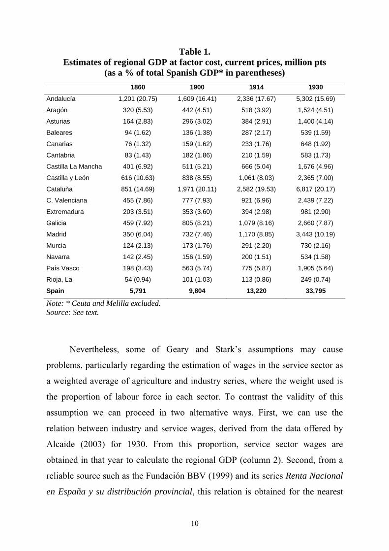
Table 1. Estimates of regional GDP at factor cost, current prices, million pts

(as a % of total Spanish GDP* in parentheses) 1860 1900 1914 1930

Andalucía 1,201 (20.75) 1,609 (16.41) 2,336 (17.67) 5,302 (15.69)

Aragón 320 (5.53) 442 (4.51) 518 (3.92) 1,524 (4.51)

Asturias 164 (2.83) 296 (3.02) 384 (2.91) 1,400 (4.14)

Baleares 94 (1.62) 136 (1.38) 287 (2.17) 539 (1.59)

Canarias 76 (1.32) 159 (1.62) 233 (1.76) 648 (1.92)

Cantabria 83 (1.43) 182 (1.86) 210 (1.59) 583 (1.73)

Castilla La Mancha 401 (6.92) 511 (5.21) 666 (5.04) 1,676 (4.96)

Castilla y León 616 (10.63) 838 (8.55) 1,061 (8.03) 2,365 (7.00)

Cataluña 851 (14.69) 1,971 (20.11) 2,582 (19.53) 6,817 (20.17)

C. Valenciana 455 (7.86) 777 (7.93) 921 (6.96) 2.439 (7.22)

Extremadura 203 (3.51) 353 (3.60) 394 (2.98) 981 (2.90)

Galicia 459 (7.92) 805 (8.21) 1,079 (8.16) 2,660 (7.87)

Madrid 350 (6.04) 732 (7.46) 1,170 (8.85) 3,443 (10.19)

Murcia 124 (2.13) 173 (1.76) 291 (2.20) 730 (2.16)

Navarra 142 (2.45) 156 (1.59) 200 (1.51) 534 (1.58)

País Vasco 198 (3.43) 563 (5.74) 775 (5.87) 1,905 (5.64)

Rioja, La 54 (0.94) 101 (1.03) 113 (0.86) 249 (0.74)

Spain 5,791 9,804 13,220 33,795

Note: * Ceuta and Melilla excluded. Source: See text.

Nevertheless, some of Geary and Stark’s assumptions may cause

problems, particularly regarding the estimation of wages in the service sector as

a weighted average of agriculture and industry series, where the weight used is

the proportion of labour force in each sector. To contrast the validity of this

assumption we can proceed in two alternative ways. First, we can use the

relation between industry and service wages, derived from the data offered by

Alcaide (2003) for 1930. From this proportion, service sector wages are

obtained in that year to calculate the regional GDP (column 2). Second, from a

reliable source such as the Fundación BBV (1999) and its series Renta Nacional

en España y su distribución provincial, this relation is obtained for the nearest

10

date available, corresponding to 1955. This proportion is then applied to the

1930 data in order to estimate the service sector wage (column 3). The

comparison of the results (Table 2) shows that the differences between the

estimates presented are in general quite small17. Thus, it seems reasonable to

suppose that Geary and Stark’s assumption about service sector wages does not

generate a great distortion18.

Table 2. Regional shares of Spanish GDP in 1930, alternative estimates.

New Estimates

(I)

Estimates using

1930 services

wages from

Alcaide

(II)

Estimates using

1955 services

wages from BBV

(III)

(II) / (I) (III) / (I)

Andalucía 5,302 15.69 5.307 15.70 5,342 15.81 1.00 1.01

Aragón 1,524 4.51 1,524 4.51 1,523 4.51 1.00 1.00

Asturias 1,400 4.14 1,340 3.96 1,324 3.92 0.96 0.95

Baleares 539 1.59 547 1.62 542 1.60 1.01 1.01

Canarias 649 1.92 619 1.83 632 1.87 0.95 0.97

Cantabria 583 1.73 595 1.76 587 1.74 1.02 1.01

Castilla La Mancha 1,676 4.96 1,724 5.10 1,733 5.13 1.03 1.03

Castilla y León 2,365 7.00 2,615 7.74 2,631 7.79 1.11 1.11

Cataluña 6,817 20.17 6,654 19.69 6,595 19.51 0.98 0.97

C. Valenciana 2,439 7.22 2,473 7.32 2,460 7.28 1.01 1.01

Extremadura 981 2.90 996 2.95 1,010 2.99 1.02 1.03

Galicia 2,660 7.87 2,803 8.29 2,781 8.23 1.05 1.05

Madrid 3,443 10.19 3,358 9.94 3,366 9.96 0.98 0.98

Murcia 730 2.16 747 2.21 777 2.30 1.02 1.06

Navarra 534 1.58 482 1.43 496 1.47 0.90 0.93

País Vasco 1,906 5.64 1,757 5.20 1,739 5.14 0.92 0.91

Rioja, La 249 0.74 256 0.76 258 0.76 1.03 1.04

Spain 33,795 100 33,795 100 33,795 100 1.00 1.00

17 Only Castilla y León shows discrepancies slightly above 10%, suggesting that, in this region, the wage for the service sector could be underestimated. 18 In this respect, Geary and Stark (2002) use their methodology to replicate the official incomes by country in the 1970s, when the whole set of data necessary exists. They conclude that ‘the errors are within those tolerated in national income accounting’, pp. 921 and 925.

11

Source: Column 1 as in Table 1; wages for Column 2 are derived from ‘Costes laborales’ and ‘Empleo asalariado’, in Alcaide (2003), pp. 270-289 and 188-207, respectively; wages for Column 3 from ‘Costes laborales’ and ‘Empleo asalariado’, in BBV (1999), pp. 122-149 and 178-205, respectively.

However, this estimation of the service sector wages may present some

inaccuracies in the results obtained for Madrid19, an economy strongly

dependent on tertiary activities20. It is therefore worth testing whether or not the

wages estimated for Madrid in the service sector are appropriate. In order to do

so, we use the wages quoted by Reher and Ballesteros (1993) for Madrid

municipal workers belonging to twelve different occupations21. These data are

only available as an index number of the average wage for these twelve

categories, based on 1913, and not in monetary units. The evolution of both

magnitudes in the two first years (1900 and 1913) is quite similar, and only in

the corresponding observation for 1930 is the discrepancy significant. Service

sector wages seem to have experienced a lower increase than assumed. The next

step is to apply the growth derived from the series by Reher and Ballesteros

between 1914 and 1930 to the wages previously estimated for Madrid in 1914.

By doing so, we find the new service sector wage in the capital of Spain for

1930 falls from 7.32 to 6.12 pesetas per day. As a consequence, the new GDP

estimation, with wages corrected, shows that Madrid’s participation in Spanish

GDP falls by one percentage point. Furthermore, in terms of GDP per capita in

1930, Madrid no longer heads the Spanish ranking, losing first place to

Catalonia22.

19 Although differences in wages for Madrid in Table 2 are small (2%). 20 Between 1860 and 1920, around half of the active population in Madrid worked in the service sector. That proportion rose to 60% in the 1930 Census of Population. 21 These occupations are: officer, unskilled labourer, foreman, assistant, manual worker, sweeper, night watchman, secretary, government employee, dean, doctor and medical assistant. 22 See Table A.1 in the Appendix.

12

In Table 3, the new estimates of regional GDP are compared to figures

offered previously by other authors. The comparison is drawn, for the matching

years, with the percentage of regional participation in Spanish GDP in Álvarez

Llano for 1860, 1900 and 1930, and with Alcaide’s estimates for 1930.

Table 3.

Regional structure of Spanish GDP (%), different estimates (as a proportion in parentheses)

Álvarez

Llano

1860

New

Estimates

1860

Álvarez

Llano

1901

New

Estimates

1900

Álvarez

Llano

1930

Alcaide

1930

New Estimates

1930

Andalucía 21.6 20.75 (0.96) 16.77 16.41 (0.98) 14.87 14.68 15.69 (1.05) (1.07)

Aragón 5.8 5.53 (0.95) 5.10 4.51 (0.88) 4.47 4.42 4.51 (1.01) (1.02)

Asturias 2.1 2.83 (1.35) 3.20 3.02 (0.94) 2.75 3.91 4.14 (1.51) (1.06)

Baleares 1.5 1.62 (1.08) 1.36 1.38 (1.02) 1.52 2.05 1.59 (1.05) (0.78)

Canarias 0.8 1.32 (1.64) 1.27 1.62 (1.28) 1.46 2.29 1.92 (1.31) (0.84)

Cantabria 1.5 1.43 (0.95) 1.91 1.86 (0.97) 1.34 1.42 1.73 (1.29) (1.22)

Castilla LM 7.3 6.92 (0.95) 6.51 5.21 (0.80) 6.46 5.37 4.96 (0.77) (0.92)

Cast.y León 11.4 10.63 (0.93) 11.42 8.55 (0.75) 9.51 9.68 7.00 (0.74) (0.72)

Cataluña 13.3 14.69 (1.10) 16.27 20.11 (1.24) 21.38 18.15 20.17 (0.94) (1.11)

C. Valenciana 7.7 7.86 (1.02) 7.66 7.93 (1.03) 9.72 8.53 7.22 (0.74) (0.85)

Extremadura 3.6 3.51 (0.98) 3.35 3.6 (1.07) 3.73 3.04 2.90 (0.78) (0.95)

Galicia 5.9 7.92 (1.34) 7.14 8.21 (1.15) 6.05 7.69 7.87 (1.30) (1.02)

Madrid 9.6 6.04 (0.63) 9.12 7.46 (0.82) 6.98 7.93 10.19 (1.46) (1.29)

Murcia 1.9 2.13 (1.12) 2.25 1.76 (0.78) 1.95 2.07 2.16 (1.11) (1.04)

Navarra 1.9 2.45 (1.29) 1.71 1.59 (0.93) 1.63 1.72 1.58 (0.97) (0.92)

País Vasco 3.0 3.43 (1.14) 4.00 5.74 (1.44) 5.40 6.00 5.64 (1.04) (0.94)

Rioja, La 1.1 0.94 (0.86) 0.96 1.03 (1.08) 0.78 1.05 0.74 (0.94) (0.70)

Source: Table 1; Álvarez Llano (1986), pp. 37 and 43; Alcaide (2003), pp. 250-251.

In terms of the magnitude of the difference, the evolution of the Canary

Islands, which in the new estimates presents a much better position than the one

given by Álvarez Llano, stands out. Galicia also presents an improvement,

though to a lesser degree. The discrepancy is also high in Madrid, for which the

13

previous data suggested a prominent position by the middle of the nineteenth

century, much higher than the one obtained in this study23. In contrast, by 1930

the new figures offer a more positive view for Madrid than the one offered by

Álvarez Llano. In the case of Asturias, the differences are significant in 1860,

but particularly so in the estimation for 1930, when the province shows a

substantial increase. Likewise, with these new data, growth in the two largest

industrial regions in the Spanish economy, Catalonia and the Basque Country, is

more vigorous throughout the second half of the nineteenth century. In contrast,

in the case of the two Castillas the new figures show a lower participation not

only in 1900 but in 1930 as well. Finally, other significant discrepancies arise in

certain years in Navarre, for example, in 1860, with more favourable values; by

1930, estimates for Cantabria reveal a higher income, and in that same year, the

relative participation of Valencia and Extremadura in Spanish GDP was lower

than in the previous estimates.

Discrepancies with Alcaide’s estimates in 1930 are, on the whole, smaller.

The significant differences observed in that year between our results and those

of Álvarez Llano for the regions of Asturias, Castilla La Mancha, Extremadura

and Galicia are notably reduced, and the differences with respect to other

Autonomous Communities such as the Canary Islands, Valencia and Madrid are

also smaller. However, discrepancies are still considerable in La Rioja (0.30),

Castilla y León (0.28), Madrid (0.28), Cantabria (0.22) and Balearic Islands

(0.22).

The information provided by Population Censuses, together with the new

GDP estimates for the Spanish NUTS-II regions, allow us to present the

evolution of GDP per capita over the years (Table 4). Data for 1955, 1975 and

23 One of the most recurrent criticisms of Álvarez Llano’s data is the high value offered for Madrid in 1860. See Carreras (1990), p. 10.

14

1995 have been added to the new estimates in order to present a long term view.

In this case, the data do not refer to indirect estimates, but to the figures on

Gross Added Value at factor cost provided by BBVA (1999 and 2000).

Table 4. Regional GDP per head, 1860-1995 (Spain = 100). 1860 1900 1914 1930 1955 1975 1995

Andalucía 109 86 93 80 68 72 68

Aragón 97 92 82 103 98 101 108

Asturias 82 89 85 123 111 101 87

Baleares 94 83 133 103 121 129 140

Canarias 87 84 79 81 75 83 101

Cantabria 102 125 104 112 115 102 90

Castilla La Mancha 89 70 65 64 66 78 80

Castilla y León 80 69 68 67 83 84 89

Cataluña 137 190 187 170 159 128 124

C. Valenciana 96 93 81 90 112 100 101

Extremadura 79 76 60 59 56 58 68

Galicia 69 77 79 83 70 76 83

Madrid 193 179 201 173 155 133 136

Murcia 87 57 71 79 69 83 82

Navarra 128 96 96 108 115 115 121

País Vasco 125 177 173 149 177 134 110

Rioja, La 84 101 91 85 109 105 118

CV 0.29 0.40 0.43 0.34 0.35 0.23 0.22

5 max / 5 min 1.76 2.22 2.33 2.09 2.22 1.74 1.68

max / min 0.87 0.39 0.97 0.93 1.03 1.15 0.86

Source: For 1860-1930, see text; for 1955-1975, derived from BBV (1999), pp. 120 and 284; for 1995, BBVA (2000), pp. 124 and 128.

On the whole, when considering the regional development in Spain

according to the evolution of GDP per capita in the long term, a striking aspect

is its stability over time. Table 5 shows the Autonomous Communities at the two

extremes of the ranking in the years considered. If we look at the regions that

15

have been at the top and at the bottom of the list throughout the period, we see

that Madrid, Catalonia and the Basque Country have always (barring occasional

exceptions) been among the richest regions, usually accompanied by the

Balearic Islands, Navarre and Cantabria. At the other end of the scale, six

regions have occupied the lowest positions: Extremadura, an ever-present, and

Castilla La Mancha, Murcia and Galicia, in six out of seven years, Andalusia

since the first third of the twentieth century and Castilla y León in the period

prior to the Civil War24.

These results raise several questions. Have Spanish regions converged

over the last century and a half, or has regional inequality persisted? When did

this inequality begin? How has it evolved in the long term, and in different

historical periods? Is it possible to speak of persistence in inequality patterns?

The aim of the following section is to provide some answers to these questions.

Table 5. Regions with the highest and lowest GDP per capita*. 1860 1900 1914 1930 1955 1975 1995

Madrid Cataluña Madrid Madrid País Vasco Madrid Baleares Cataluña Madrid Cataluña Cataluña Cataluña País Vasco Madrid Navarra País Vasco País Vasco País Vasco Madrid Baleares Cataluña

País Vasco Cantabria Baleares Asturias Baleares Cataluña Navarra Andalucía Rioja, La Cantabria Cantabria Cantabria Navarra Rioja, La

…………….. …………….. …………….. …………….. …………….. …………….. ……………..

Rioja, La Galicia Galicia Andalucía Galicia Murcia Galicia Asturias Extremadura Murcia Murcia Murcia CLM Murcia

CyL CLM CyL CyL Andalucía Galicia CLM Extremadura CyL CLM CLM CLM Andalucía Andalucía

Galicia Murcia Extremadura Extremadura Extremadura Extremadura Extremadura

Note: * In bold, regions that appear in at least three of the selected years. In italics, regions that appear before and after the Civil War. CyL stands for Castilla y León and CLM for Castilla La Mancha. Source: Table 4. 24 The same table for the extremes in terms of provinces (NUTS-III) can be consulted in Table A.2 in the Appendix. Stability is also present, although to a lower degree, especially at the lower end of the distribution.

16

5. Description of the evidence in the long run.

a) The evolution of regional inequalities in the Spanish literature.

The lack of data for the period prior to 1955 continues to present

problems. In 1986, Álvarez Llano estimated the distribution of the Spanish GDP

by regions for the pre-statistical period25, and although the methodology used

was not made explicit, these data have served as the basis for further studies.

Taking the figures provided by Álvarez Llano, Albert Carreras (1990) defined

the regional patterns of economic development. Using the Inequality Index of

GDP per capita, he analysed the evolution of regional inequality in Spain from a

historical perspective. He criticized Álvarez Llano’s high figures for Madrid in

1860, suggesting that the values for that year might be exaggerated26. With this

in mind, Carreras states that the tendency towards regional inequality was

constant from 1800, reaching a maximum around 1950 or 1960. From that

moment onwards, the disparities reduced and showed an inverted U-shape

evolution. By 1983, regional inequality was lower than at the starting date,

almost two centuries before.

Later, Martín (1992) characterized the tendencies of regional economic

development in Spain. Throughout the nineteenth century, a gradual widening of

economic disparities among Spanish regions seems to have taken place as a

result of the regional specialization process. Between 1900 and 1930, these

patterns intensified and the growth in productive and sectoral specialization

resulted in another widening in regional disparities, measured by the Gini Index

of the GDP per capita. Domínguez (2002) analysed regional economic

inequality in Spain over the last three centuries. Using the same data as those

used in previous studies, Domínguez suggested that the evolution shown by the

25 Álvarez Llano (1986). 26 Carreras (1990), p.10 and 15.

17

Gini Index and the Coefficient of Variation of the GDP per capita in the second

half of the nineteenth century could have led to a reduction in regional

disparities, though the other evidence available does not support this view;

indeed, other indicators such as the Williamson Index and the Industrial

Intensity Coefficient of Variation led him to affirm that regional economic

inequality rose between 1860 and 1900. This lack of consistency may have been

caused by the unreliability of the figures before 195527. The period between

1900 and 1930 was marked by a lessening in inequality that continued until

1960, with the lowest values for all indices being reached around 1970.

Furthermore, Domínguez emphasizes that between 1800 and 1990 a continuous

process of spatial concentration in production took place in a decreasing number

of regions, corroborating German’s (1996) idea of regional polarization in

Spanish economic growth.

In a recent study, Rosés and Sánchez-Alonso (2004) build a new dataset

of regional real wages for three different occupations (agrarian labourers,

unskilled urban workers and urban industrial workers). They conclude that

wages converged substantially from 1850 to 1914. Only in the aftermath of the

WWI did wage differentials increase and during the 1920s real wage

convergence across Spanish provinces returned.

b) Empirics: the new evidence.

In recent decades economic growth and convergence between countries

has become an important topic in the literature. From the methodological point

of view, most of the research carried out in this area has rested on the idea of the

existence of β-convergence and σ-convergence28. As regards the first concept,

27 According to Domínguez, this view is reinforced with the evolution of the Physical Quality of Life Index (PQLI). As we go back in time, the correspondence between this indicator and GDP per capita reduces. Domínguez (2002), pp. 70-80. 28 Barro and Sala-i-Martín (1992).

18

there is an inverse relation between the growth rate and the initial income per

capita, so for a set of economies the growth rate of the countries shows a

tendency towards convergence; that is, the initially poorest countries will grow

faster than the richest ones. Besides, the existence of σ-convergence implies a

reduction of the income per capita dispersion over time for a sample of

countries. If instead of countries the study focuses on regions in the same State,

the convergence would take place at a faster pace, as they are more

homogeneous units which have historically shared the same institutions and

economic policy. A first approach to the measurement of the degree of σ-

convergence is the evolution in the Coefficient of Variation (Table 4). A

reduction in the coefficient over time would mean the existence of σ-

convergence. In order to obtain a long term view helpful for the examination not

only of the origin of regional inequality in income per capita but also of its

persistence up to the present day, the analysis maintains the observations for the

second half of the twentieth century up to 1995.

Between 1860 and 1900, the dispersion of income per capita increased

and continued to do so until 1914. From 1914 onwards, this process was

interrupted and the coefficient of variation began to fall. Therefore, Spanish

regions converged to a certain extent until 1930. Nevertheless, this convergence

was temporary; in the first years of the Franco regime the coefficient of

variation remained almost stable, around 0.35, still above its initial 1860 value.

Strong convergence was recorded from 1955 to 1975, as witnessed by the

significant reduction in the coefficient. However, from that date onwards and

over the last twenty years in this study the coefficient showed a tendency to

stagnate29.

29 The coefficient shows the same evolution at a province level, NUTS-III.

19

Quah (1993, 1996) has suggested an alternative approach to the study of

convergence between economies, based on the evolution of the distribution of

income per capita on the whole, and known as distribution dynamics. Following

Quah, we analyse the new evidence, first by plotting the kernel diagrams of the

income per capita distribution. Kernel density diagrams allow an evaluation of

the degree of convergence by studying the shape of the distribution at a specific

point in time. From now on, and with a few exceptions in order to increase the

number of observations, the analysis will include data for the 49 Spanish

provinces (NUTS-III) between 1860 and 1995. Figures have been normalized on

the Spanish GDP per capita (with the average taking a value of 1). Therefore,

the kernel diagrams in Figure 1 describe the relative distribution of provinces

around the sample average for the selected years30.

In figure 1, 1860 is the clearest peak, showing a greater number of regions

around the Spanish average. However there is a clear reduction between 1860

and 1900. In this analysis, convergence in the income is measured by the height

of distribution: a flatter distribution suggests a greater dispersion from the

average, reflecting an increase in regional inequality, or divergence. Therefore,

there seems to have been a slight convergence between 1900 and 1930, although

the process was later interrupted, since 1955 presents a minimum value.

Convergence was continuous from that year onwards, though the distribution in

1995 still reached a maximum close to that of 1930. Another notable feature of

the curves is that they moved to the left with respect to the initial year of 1860.

This represents a greater density of provinces grouped around a value

increasingly lower with regard to the average sample. This evolution does not

begin to be corrected until 1975.

30 I used the Epanechnikov Kernel with Silverman’s optimal bandwidth. The distribution of the new estimates for 1860-1930 can be consulted in Figure B.1 in the Appendix.

20

Figure 1. Kernel densities (GDP per head in 49 Spanish provinces, 1860-1995).

0,0

0,5

1,0

1,5

2,0

2,5

3,0

0,0 0,5 1,0 1,5 2,0 2,5 3,0

1860190019141930195519751995

Finally, in 1860 we observe a tendency in a group of regions to cluster

around an income per capita level 1.8-2 times higher than the Spanish average,

presenting a peak at the high end of the distribution. In 1900, two subgroups of

regions appear clustering around 1.6-2 and 2.4-2.8 times the Spanish average;

these two peaks are less pronounced. From that point on, the tendency starts to

decrease and by 1975 no twin peaks are seen at the high end.

Nevertheless, the kernel diagrams give information on what the whole

distribution looks like over different periods of time, but tells us nothing about

the mobility within the distribution. If the aim is to analyse convergence

between Spanish regions, we need to know if relatively rich or poor regions

continued to be rich or poor over time. Therefore, the analysis of mobility is of

great importance. In order to illustrate the intra-distribution movement, we

21

define five income states (much below average, below average, average, above

average, and much above average), in which income state 1 corresponds to the

lowest income level and income state 5 to the highest31.

A first step in the study of the mobility within the distribution is to assign

the different economies to these five income states in the years selected, and

then to count the changes in income states. Three historical periods are taken

into consideration (1860-1900, 1900-1930, and 1955-1995). In order to simplify

the analysis, we carry out the exercise for NUTS-II Spanish regions. Figure 2

shows the distribution of regions by income state in different years. The

horizontal axis shows the income states, and the vertical axis indicates the

number of economies included in each one. Further, the matrices show the

movements of regions between income states for each pair of dates considered.

These results can be interpreted as follows. In 1860 there were five regions in

income state 4. By 1900, two regions had fallen into income state 3, and one had

risen to income state 5. In addition, one region initially in income state 3 in 1860

had risen to income state 4 in 1900, and one region in income state 5 in 1860

moved to income state 4 in 1900, leaving four economies in income state 4 in

190032.

The results show that mobility was an important feature in all periods,

particularly so during the period 1900-1930, when ten out of the seventeen

Autonomous Communities moved from their initial income state. The mobility

in the other two periods considered was almost equally pronounced and in both

cases more than half of the regions transited to a different income state.

31 The normalized observations are ranked from highest to lowest and split into five equally large income states, where each state contains the same number of regions. See Epstein et al. (2003), footnote 11, p. 84. The cell partition is derived by Quah’s TSRF program. 32 The regions that experienced these changes in income state are shown in Table A.3 in the Appendix.

22

Moreover, movements of more than one income state can be observed in all

periods. Between 1860 and 1900, the only economy which experienced such

movements fell to a lower income level; between 1900 and 1930, two rises were

recorded; and between 1955 and 1995 two out of the three regions that moved

more than one income state ended up in a higher income state.

In 1860-1900, mobility was also concentrated in middle income states,

since five out of the nine transitions took place in income state 3, which would

be a sign of divergence. Between 1900 and 1930 only two out of the ten

movements occurred in the average income state. On the other hand, four

transitions ended up in the average income state. Over the last period, the

starting situation had reversed; there were no movements in income state 3 and

transitions were concentrated at the higher and lower ends. Moreover, five

transitions ended up in income state 3 during this period. This shows the

existence of convergence forces.

23

Figure 2. Empirical distribution and mobility by income state for 17 Spanish regions, NUTS-II, 1860-1995.

0

1

2

3

4

5

6

7

8

1 2 3 4 5

1860

0

1

2

3

4

5

1 2 3 4 5

1900

0

1

2

3

4

5

6

7

1 2 3 4 5

1930 Number of moves between

income states, 1860 to 1900. Number of moves between income states, 1900 to 1930

1 2 3 4 5 1 2 3 1 3 14 2 15 1

1 2 3 4 51 12 3 13 1 14 25 1

0

1

2

3

4

5

6

7

1 2 3 4 5

1955 0

1

2

3

4

5

6

7

1 2 3 4 5

1995 Number of moves between

income states, 1955 to 1995. 1 2 3 4 5

1 1 1 2 2 1 3 4 1 1 5 1 1

24

Finally, the probability of falling into a lower income state seems to have

been higher in the initial stages of economic development. Between 1860 and

1900, seven out of nine transitions ended up in an inferior income state, but

between 1900 and 1930, the probability of falling into a lower income state was

more similar to that of rising to a higher income state. Between 1955 and 1975,

two thirds of transitions were to a higher income state and only one third were to

a lower one. In this case, increases were concentrated in the lowest income

regions, whereas the falls in income states were experienced by higher income

regions, emphasizing the idea of convergence over this period.

However, this first empirical approach to the mobility within the

distribution is purely descriptive and has to be considered with care. From now

on, following Quah’s suggestion, a more formal approach is proposed through

the distribution dynamics and transition probability matrices. In order to use all

the information available, the analysis is again based on the 49 Spanish

provinces33. Starting from the five income states defined above, we first derive

the transition probability matrix, which shows the average probability of

provinces to move from an income state to another. The aim is to test the

existence of mobility within the distribution. Second, the matrix obtained may,

through continuous iteration, result in a long term equilibrium where a further

iteration would not have any effect. This is known as the ergodic distribution,

which shows the shape of the distribution in the long run. In order to calculate

the transition probability matrices and the ergodic distribution, we use the Time

Series Random Field (TSRF) econometric shell developed by Quah.

33 The study includes six years. In order to homogenize the periods and analyse transitions in income states, the observation for 1914 has been excluded. Nevertheless, the time span of the periods is not the same over time and therefore the likelihood of a region making a transition is larger between 1860 and 1900 than it is between 1955 and 1975. Of course, the same yearly space between the cross sections would be the desirable situation. However, the time span of transitions is restricted to the availability of the data. A total of 294 observations were made.

25

The vertical axis illustrates the initial income states of the provinces,

whilst the rows of the matrix show the probability that, on average, an economy

in an income state will move to another income state over time. Thus, each of

the rows in the matrix will add up to 1. Two main features should be considered

when dealing with the matrix: persistence and mobility. Persistence is given by

the elements on the diagonal of the matrix, reflecting the probability that a

province in an income state remains in the same income state over time.

According to Table 6, the degree of persistence is higher at both the

higher end (75%) and the lower end (58%) than in middle income states34.

Further, in both cases, the probability of remaining in the initial income state is

higher than that of moving to a different one. In contrast, intermediate income

states 2, 3 and 4 show a lower degree of persistence, and thus, greater

mobility35.

When analysing mobility, stress should be placed on the values outside

the diagonal, which give us the probability that an economy in an initial income

state will change to a different income state over time. In this case, the upper

triangle represents the probability of mobility towards higher income states, and

the lower triangle, the transitions towards lower income states. As we have seen,

the probability of being much above average income is higher than that of being

much below average income on the diagonal. However, the probability of a top-

ranked province falling behind (19%) is lower than the probability of a province

much below average income rising (34%). Thus, it is easier to leave income

34 Since the periods considered are quite large and thus the probability of transition between income states is higher, it is possible to assert, according to the values reached in the extremes of the matrix diagonal, that persistency seems to be important. 35 Although the probability of remaining in income state 4 (56%) is very similar to that of remaining in income state 1 (58%).

26

state 1 than to leave income state 5. Further, there exists the possibility of an

economy initially in income state 1 ending up in income state 4 (2%).

From state 2, a representative economy is more likely to go up to income

state 3 (28%) than to fall (24%). It could even go ahead to income state 4 (6%).

A province in income state 3 is more likely to move up an income state (26%)

than to move down a state (15%). This pattern also applies for a province in

income state 4 (21% and 15%), although the possibility of going back three

income states also exists (2%). In general, for middle income categories, the

probability of falling into a lower income state is always lower than that of

moving to a higher income state.

Table 6. Transition probability matrix (GDP per head relative to Spanish average).

1 2 3 4 5

1 0,58 0,34 0,06 0,02 0,00

2 0,24 0,42 0,28 0,06 0,00

3 0,07 0,15 0,48 0,26 0,04

4 0,02 0,06 0,15 0,56 0,21

5 0,00 0,00 0,06 0,19 0,75

Ergodic

Distribution: 0,137 0,161 0,202 0,254 0,247

1860: 0,102 0,082 0,347 0,286 0,184

The next stage in the analysis is to derive the ergodic distribution through

continuous iteration of the transition probability matrix until the steady state is

reached. Therefore, the dynamics inherent to the system can be studied and

conclusions about the existence of convergence in the long term may be

reached. The ergodic distribution shows what the map of Spain would look like

if the probabilities of transition of the provinces remained unchanged in time:

27

the ergodic distribution reports the equilibrium proportion of economies falling

in each of the five relative income states.

The existence of convergence in the long run would require an ergodic

distribution where the provinces were mainly located around income state 3,

defined as the average income state. On the other hand, if the distribution tended

to be flat among all income states, this would be a sign of divergence.

Nevertheless, here, the results show that, in the long run equilibrium, as we rise

in the income scale from 1 to 5, the proportion of provinces in the higher income

states increases, with income state 4 including the greater number of

provinces36. A distribution of this type does not reflect convergence. Further,

two different plateaux can be observed: first, for the lower income states, where

50% of the provinces are found in income states 1, 2 and 3 in the long run, and

second, for the provinces in higher income states, with the remaining half of the

provinces distributed in income states 4 and 5.

6. Concluding remarks.

The recent study by Geary and Stark (2002) has established a

methodology for estimating regional GDP which can be applied to other

economies such as the Spanish economy. In the case of Spain, this application is

of particular interest due to the inexistence of reliable data for the territorial

distribution of GDP before 1955.

After explaining the process and the treatment of the sources used, we

tested the robustness of certain implicit assumptions regarding Geary and 36 Although the transition probability description suggests incomes tending towards extremes at both high and low endpoints.

28

Stark’s methodology. In particular, we tested the assumption that sector service

wages are proxied by a weighted average of agriculture and industry series,

finding that it does not greatly distort the estimates.

Likewise, the new series are analysed by comparing them to other

available estimates, such as those in Álvarez Llano (1986) and Alcaide (2003).

From the comparison, certain constants can be inferred which show that the

results in the present paper differ from those previously obtained.

Using the new estimates, a series of descriptive exercises are proposed for

an analysis of the historical dynamics of the geographical distribution of income

and the existence of convergence in the long run. Quah’s work is the reference.

Looking at the shape of the kernel distribution, an increase in regional inequality

is observed between 1860 and 1900 which is much flatter in the later year. The

empirical analysis of the distribution also shows a certain mobility over this

period. This mobility mainly affected the middle income regions with a clear

tendency to fall to a lower income state.

Between 1900 and 1930, the kernel diagrams reveal the existence of two

subperiods, divided by the corresponding observation for 1914. Up to 1914, the

distribution increases in height and so we can speak of convergence. However,

in 1930, the distribution is slightly lower, revealing stagnation in the process of

convergence. This is the period of highest mobility within the distribution, as

well as a period with a lower number of transitions in the average income state

than in the previous years. Downward mobility is still important.

The evolution of kernel density distribution suggests a tendency towards

convergence in the period from 1955 to 1995. This is also a period with a certain

mobility, although in this case, mobility is centred in the higher and lower

29

extremes of the sample. Two thirds of the transitions tend to occur towards

higher income states, and concentrate in the lower income provinces. Downward

mobility is important in the higher income states, reinforcing the view of a

convergence period.

The transition probability matrices show a greater persistence in the

extremes of the distribution. Thus, richer provinces remained rich and the poorer

tended to remain poor, although the probability of leaving income state 1 was

higher than the probability of leaving income state 5. In the middle incomes,

mobility was more important, though the probability of falling to a lower

income was always lower than the probability of rising to a higher income state.

As regards the ergodic distribution, the long run tendency shows that half of the

provinces would be found in the two higher income states. The remaining half

would be distributed between the much below average (13.7%), below average

(16.1%) and average income states (20.2%). This situation does not reflect

convergence in the long run.

To conclude, one point should be stressed. The main contribution of this

paper is the presentation of new regional and provincial GDP data set for Spain

between 1860 and 1930 following Geary and Stark (2002). Recently, Crafts

(2005) has suggested a way of refining this methodology by including non-wage

income in the estimation using the regional distribution of income tax. The next

step forward in the research is to improve the new estimates along the lines that

Crafts suggests.

30

References

Álvarez Llano, R. (1986): “Evolución de la estructura económica regional de

España en la historia: Una aproximación”, Situación, 1, pp. 5-61.

Alcaide Inchausti, J. (2003): Evolución económica de las regiones y provincias

españolas en el siglo XX, Fundación BBVA, Bilbao.

Bairoch, P. (1976): “Europe’s Gross National Product: 1800-1975”, Journal of

European Economic History, vol. 5, (Fall), pp. 273-340.

Barro, R. and Sala-i-Martín (1992): “Convergence”, Journal of Political

Economy, vol.100, nº 21, pp. 223-251.

Beckerman, W. and Bacon, R (1966): “International comparisons of income

levels: a suggested new measure”, Economic Journal, vol. 76, (September), pp.

519-536.

BBV (1999): Renta Nacional de España y su distribución provincial. Serie

homogénea. Años 1955 a 1993 y avances 1994 a 1997, vols. I-II, Fundación

BBV, Bilbao.

BBVA (2000): Renta Nacional de España y su distribución provincial. Año

1995 y avances 1996-1999, Fundación BBVA, Bilbao.

Bringas Gutierrez, M. A. (2000): La productividad de los factores en la

agricultura española (1752-1935), Banco de España.

31

Carreras, A. (1990): “Fuentes y datos para el análisis regional de la

industrialización española”, in Carreras A., Nadal J., (eds), Pautas regionales de

la industrialización española (siglos XIX y XX), Ariel, Barcelona, pp. 3-20.

Crafts, N.F.R. (1983): “Gross National Product in Europe 1870-1910: some new

estimates”, Explorations in Economic History, vol.20, (October), pp. 387-401.

Crafts, N.F.R. (2005): “Regional GDP in Britain, 1871-1911: Some estimates”,

Scottish Journal of Political Economy, vol.52, No. 1, pp. 54-64.

Domínguez, R. (2002): La riqueza de las regiones. Las desigualdades

económicas regionales en España, 1700-2000”, Alianza, Madrid.

Epstein, P., Howlett, P., and Schulze, M.S. (2003): “Distribution dynamics:

stratification, polarization and convergence among OECD economies, 1870-

1992”, Explorations in Economic History, 40, pp. 78-97.

Esposto, A.G. (1997): “Estimating regional per capita income: Italy, 1861-

1914”, Journal of European Economic History, 26, pp. 585-604.

Geary, F., and Stark, T. (2002): “Examining Ireland’s post-famine economic

growth performance”, The Economic Journal, No. 112, pp. 919-935.

Germán, L. (1996): “Crecimiento económico, disparidades y especialización

regional en España (siglos XIX-XX)”, Cuadernos Aragoneses de Economía, pp.

203-212.

32

Good, D. (1994): “The economic lag of Central and Eastern Europe: Income

estimates for the Habsburg successor states, 1870-1910”, Journal of Economic

History, vol.54, No. 4, (December), pp. 869-891.

Instituto Geográfico y Estadístico (1903): Estadística de la emigración e

inmigración de España, 1896-1900, Ministerio de Instrucción Pública y Bellas

Artes, Madrid.

Madrazo, S. (1984): El sistema de transportes en España, 1750-1850, Turner,

Madrid.

Martín, M. (1992): “Pautas y tendencias de desarrollo económico regional en

España: una visión retrospectiva”, in J.L. García Delgado and A. Pedreño, dirs.,

Ejes territoriales de desarrollo: España en la Europa de los noventa, Madrid,

pp. 133-155.

Ministerio de Trabajo, Comercio e Industria (1927): Estadística de salarios y

jornadas de trabajo referida al período 1914-1930, Madrid.

Moral Ruiz, J. (1979): La agricultura española a mediados del siglo XIX, 1850-

1870, Ministerio de Agricultura, Madrid.

Prados de la Escosura, L. (2000): “International comparisons of real product,

1820-1990: an alternative data set”, Explorations in Economic History, 37, pp.

1-41.

Prados de la Escosura, L. (2003): El Progreso Económico de España 1850-

2000, Fundación BBVA, Bilbao.

33

Quah, D. (1993): “Empirical cross-section dynamics in economic growth”,

European Economic Review, 37, pp. 426-434.

Quah, D. (1996): “Regional convergence clusters across Europe”, European

Economic Review, 40, pp. 951-958.

Quah, D. (1997): “Empirics for growth and distribution: Stratification,

polarization and convergence clubs”, Journal of Economic Growth, 2, pp. 27-59.

Rosés, J.R. and Sánchez-Alonso, B. (2004): “Regional wage convergence in

Spain 1850-1930”, Explorations in Economic History, 41, pp. 404-425.

Sánchez Alonso, B. (1995): Las causas de la emigración española 1880-1930,

Alianza Editorial, Madrid.

Schulze, M-S. (2000): “Patterns of growth and stagnation in the late nineteenth

century Habsburg economy”, European Review of Economic History, 4, pp.

311-340.

Silvestre Rodríguez, J. (2003): Migraciones interiores y mercado de trabajo en

España, 1877-1936, tesis doctoral, Universidad de Zaragoza.

Simpson, J. (1995): “Real wages and labour mobility in Spain, 1860-1936”, in

Scholliers, P., Zamagni, V., (eds), Labour reward, Edward Elgar, pp. 182-200.

Williamson, J. (1965): “Regional inequality and the process of national

development: a description of the patterns”, Economic Development and

Cultural Change, 13:4 Part II, pp. 3-84.

34

Appendix

Table A.1. 1913=100 Service sector wages, Madrid

Reher and Ballesteros New (pts./day)

1900 78.68 77.29

1914 100.55 100.00 2.94

1930 209.18 248.50 6.12

Madrid Madrid

Service sector wage estimate = 7.32 Service sector wage corrected = 6.12

GDP 1930 (mil. pts.) % GDP 1930 (mil. pts.) %

3,443 10.19 3,084 9.12

GDP per capita, 1930

Madrid, service sector wage corrected

= 6.12

GDP per capita,1930

Madrid, service sector wage estimate

= 7.32

Cataluña 172 Madrid 173

Madrid 155 Cataluña 170

País Vasco 151 País Vasco 149

Asturias 125 Asturias 123

Cantabria 113 Cantabria 112

Navarra 109 Navarra 108

Aragón 104 Aragón 103

Baleares 104 Baleares 103

C. Valenciana 91 C. Valenciana 90

Rioja, La 86 Rioja, La 85

Galicia 84 Galicia 83

Canarias 82 Canarias 81

Andalucía 81 Andalucía 80

Murcia 80 Murcia 79

Castilla y León 67 Castilla y León 67

Castilla La Mancha 65 Castilla La Mancha 64

Extremadura 60 Extremadura 59

Spain 100 Spain 100

35

Table A.2. Provinces with the highest and lowest GDP per capita*. 1860 1900 1914 1930 1955 1975 1995

Barcelona Barcelona Barcelona Barcelona Vizcaya Álava Gerona Madrid Guipúzcoa Guipúzcoa Madrid Barcelona Guipúzcoa Baleares

Cádiz Vizcaya Madrid Vizcaya Guipúzcoa Madrid Madrid Vizcaya Madrid Cádiz Guipúzcoa Madrid Tarragona Álava Navarra Gerona Gerona Zaragoza Álava Baleares Tarragona

……………. ……………. ……………. ……………. ……………. ……………. …………….

Cáceres Lugo Teruel Cáceres Orense Cáceres Córdoba

Pontevedra Murcia Granada Granada Cáceres Jaén Cádiz

Zamora Ávila Soria Cuenca Jaén Orense Jaén

León Cáceres Zamora Zamora Granada Granada Granada Lugo León Cáceres Salamanca Almería Badajoz Badajoz

Note: * In bold, regions that appear in at least three of the selected years. In italics, regions that appear before and after the Civil War. CyL stands for Castilla y León and CLM for Castilla La Mancha. Source: Table 4.

Figure B.1. Kernel densities (GDP per head in 49 Spanish provinces, 1860-1930).

0,0

0,5

1,0

1,5

2,0

2,5

3,0

0,0 0,5 1,0 1,5 2,0 2,5 3,0

1860190019141930

36

Table A.3. Changes in income states, Spanish regions. 1860 1900 1860-1900 1900 1930 1900-1930 1955 1995 1955-1995

Andalucía 1.09 (4) 0.86 (3) -1 0.86 (3) 0.80 (3) 0.68 (3) 0.68 (2)

Aragón 0.97 (4) 0.92 (4) 0.92 (4) 1.03 (4) 0.98 (4) 1.08 (4)

Asturias 0.82 (3) 0.89 (3) 0.89 (3) 1.23 (5) +2 1.11 (4) 0.87 (3) -1

Baleares 0.94 (4) 0.83 (3) -1 0.83 (3) 1.03 (4) +1 1.21 (5) 1.40 (5)

Canarias 0.87 (3) 0.84 (3) 0.84 (3) 0.81 (3) 0.75 (2) 1.01 (4) +2

Cantabria 1.02 (4) 1.25 (5) +1 1.25 (5) 1.12 (4) -1 1.15 (5) 0.90 (3) -2

Castilla La Mancha 0.89 (3) 0.70 (2) -1 0.70 (2) 0.64 (1) -1 0.66 (1) 0.80 (3) +2

Castilla y León 0.80 (3) 0.69 (2) -1 0.69 (2) 0.67 (1) -1 0.83 (3) 0.89 (3)

Cataluña 1.37 (5) 1.90 (5) 1.90 (5) 1.70 (5) 1.59 (5) 1.24 (5)

C. Valenciana 0.96 (4) 0.93 (4) 0.93 (4) 0.90 (3) -1 1.12 (4) 1.01 (4)

Extremadura 0.79 (3) 0.76 (2) -1 0.76 (2) 0.59 (1) -1 0.56 (1) 0.68 (2) +1

Galicia 0.69 (2) 0.77 (2) 0.77 (2) 0.83 (3) +1 0.70 (2) 0.83 (3) +1

Madrid 1.93 (5) 1.79 (5) 1.79 (5) 1.73 (5) 1.55 (5) 1.36 (5)

Murcia 0.87 (3) 0.57 (1) -2 0.57 (1) 0.79 (3) +2 0.69 (2) 0.82 (3) +1

Navarra 1.28 (5) 0.96 (4) -1 0.96 (4) 1.08 (4) 1.15 (5) 1.21 (5)

País Vasco 1.25 (5) 1.77 (5) 1.77 (5) 1.49 (5) 1.77 (5) 1.10 (4) -1

Rioja, La 0.84 (3) 1.01 (4) +1 1.01 (4) 0.85 (3) -1 1.09 (4) 1.18 (5) +1

Total Trans. 9 10 9

Simple Trans.* 6+2 6+2 2+4 Double Trans.* 1+0 0+2 1+2

Note: * In bold, downward mobility; in italics, upward mobility.

37