DOCUMENTATION FILE Tonzi Ranch Document August 10, 2006 Written and Edited by D. Baldocchi AmeriFlux Site: Ione, CA

1. TITLE Measuring and Modeling Carbon, Water Vapor and Energy Exchange over Grassland and Tree/Grass Ecosystems PROJECT SUMMARY Western savanna ecosystems are among the most complex ecosystems to be studied by biometeorologists. They are horizontally and vertically heterogeneous, they experience summer water deficits, and they rely on a multiple plant functional approaches to acquire carbon and manage water loss. At present, savanna ecosystems are poorly represented in the AmeriFlux network. Yet, savannas constitute a major ecosystem and are analogs for studying how the carbon metabolism of ecosystems will respond to environmental perturbations. We are studying the roles of climate and ecosystem structure and functionality on carbon and water fluxes of an oak/grass savanna and a grassland. This study will provide information on how broadleaved, deciduous forests, in AmeriFlux, respond to changes in soil moisture. It will broaden the range of climate variables, canopy structure and functionality that is currently under study by the network. The eddy covariance method will be used to measure flux densities of CO2 and water vapor. Portable eddy flux systems will be deployed in the surface layer and understory of the savanna to augment the tower-based flux measurements. Physiological capacity, sap flow and soil-root respiration will be measured to evaluate fluxes associated with constituent compartments. Our objectives are to assess: 1) the relative contributions of vegetation and the soil on CO2 and water vapor exchange; 2) spatial variability of understory fluxes; 3) the impact of sloping terrain on the interpretation of flux covariances. A biophysical gas exchange model (CANVEG) and a Lagrangian footprint model will be used to synthesize and interpret the data. 2.0) INVESTIGATOR(S) 2.1) Investigator(s) Name And Title.

Dennis Baldocchi, Principal Investigator, Professor of Biometeorology, Department of Environmental Science, Policy and Management, 151 Hilgard Hall University of California, Berkeley, CA 94720, Baldocchi@nature.berkeley.edu; 510-642-2874 (phone); 510-643-5098 (fax) Collaborators and Technical Assistance: Biometeorology Lab

Dr. Siyan Ma, Associate Specialist Dr. Jorge Curiel-Yuste, postdoctoral scientist Mr. Ted Hehn, Developmental Technician.

Dr. Todd Dawson, IB/ESPM, UC Berkeley Dr. Kevin Tu, IB, UC Berkeley Dr. John Battles, ESPM, UC Berkeley Dr. Bill Frost, AES/UC Davis Graduate Students: Jessica Cruz Osuna Qi Chen Xingyuan ‘Lorraine’ Chen Gretchen Miller Youngryel Ryu Undergraduate Simon Wong Former Collaborators and Graduate Students: Dr. Josh Fisher, Oxford Dr. Liukang Xu, LICOR Dr. Jianwu Tang, Univ Minnesota Dr. Lianhong Gu, ORNL Dr. Nancy Kiang, NASA/GISS Dr. Francesca Ponti, University of Bologna Landholders: Mr. Russell Tonzi Mr. Fran Vaira 2.2) Contacts (For Data Acquisition and Production Information).

Dennis Baldocchi, Department of Environmental Science, Policy and Management, 151 Hilgard Hall University of California, Berkeley, CA 94720, Baldocchi@nature.berkeley.edu; 510-642-2874 (phone); 510-643-5098 (fax) 2.3) Requested Form of Acknowledgement. Dennis Baldocchi, Department of Environmental Science, Policy and Management, 137 Mulford Hall University of California, Berkeley, CA 94720, Baldocchi@nature.berkeley.edu; 510-642-2874 (phone); 510-643-5098 (fax) Scalar and energy flux data (e.g. CO2, water vapor, sensible heat and solar energy): Co-authorship if there is extensive use of the data to validate models. Acknowledgement if only few data are used to make a supporting point. Meteorological data: Acknowledgment. Acknowledgement: Field data obtained and prepared by Dennis Baldocchi and Liukang Xu (until April, 2004) or Siyan Ma (after May, 2004), Department of Environmental Science, Policy and Management, 151 Hilgard Hall University of California, Berkeley, CA 94720, Baldocchi@nature.berkeley.edu; 510-642-2874 (phone); 510-643-5098 (fax) 3. INTRODUCTION 3.1) Objective/Purpose. The objective of this research is to measure and model air-surface exchange rates of water vapor, sensible heat and CO2 over a grazed grassland and oak/grass savanna and to study the abiotic and biotic factors that control the fluxes of scalars in this landscape. Scalar flux densities were measured with tower-mounted measurement systems. The work to be done addresses three overarching objectives. The first objective of the proposed work is:

to establish a new AmeriFlux site and measure and model the biotic and abiotic factors that govern carbon, water and energy exchange of a grassland and an grass/oak savanna over the time scales of hours to days and years.

The second objective of the proposed work is:

to study the impact of heterogeneous canopies and sloping terrain on the measurement and modeling of carbon and water fluxes across a gradient of vegetation and soil.

The third objective of the proposed work relates to flux footprints and the partitioning of fluxes between the vegetative and soil components. We intend to study:

a) the temporal and spatial patterns of soil respiration, evaporation, micrometeorology, canopy structure and energy exchange; b) use this information to parameterize a two dimensional and multi-layer footprint model; c) combine information on wind direction, flux footprints and biomass transects to evaluate the flux climatology of the site.

As we enter the newest stage of work, we will expand our scope to understand how trends and inter-annual variations in climate affect carbon and water exchange between terrestrial ecosystems and the atmosphere on a decadal time scale. We propose a study that will investigate and quantify the dynamics of net carbon dioxide exchange between the biosphere and atmosphere, which are triggered by such critical features as switches, pulses, lags, and acclimation. We will upscale the fluxes in space and time with remote sensing and regional weather data. Upscaling will be accomplished in the following manner. First, periodic measurements of high resolution spectral reflectance will be made with a spectral radiometer and continuous measurements of vegetation indices (NDVI and PRI) will be made with an LED spectrometer developed in our lab. Second, relationships between vegetation indices and carbon fluxes will be derived from the field observations. And third, we will apply these algorithms to vegetation indices obtained from MODIS and produce ecosystem-scale estimates of carbon assimilation. We will add a new component to our project that will compare long term eddy flux measurements against changes in stand biomass and soil carbon. These will be based on a sequence of LIDAR measurements and biometry field sampling. RESEARCH HYPOTHESES

Based on the science and objectives we have introduced and discussed, many interesting questions arise that can form the basis of this research project. Key questions we intend to address in relation to measuring and modeling carbon and water fluxes of a grassland and an oak/grass savanana. They relate to the functionality and variability of carbon and water vapor fluxes in time and space.

Questions relating to functionality include:

1) How do year-to-year variations in annual rainfall, due to the presence of El Niño or La Niña, affect the carbon and water balances of these systems?

2) How do the carbon and water vapor fluxes of an annual grassland differ from a nearby grass/oak savanna over a spectrum of time scales?

3) How does the mixed grass/tree landscape coordinate the use of water for the gain of carbon over the course time?

Along the vertical spatial axis, we intend to ask:

1) How do vertical differences in physiological capacity, plant architecture and the physical environment integrate to the canopy dimension?

2) What are the relative roles of soil and vegetation on mass and energy exchange?

The main hypotheses we intend to ask with regard to horizontal variability include:

1) Can a flux footprint model be used with a one-dimensional biophysical model to assess fluxes of water and carbon across a patchy landscape or must we consider the advection/diffusion equation in two dimensions?

2) How does sloping terrain affect the conventional measurement of eddy fluxes over short vegetation? Does CO2 leak out of the control volume as air drains out of the system close to the ground?

3) What are the relative contributions of biodiversity (a mix of species and functional types) on land-atmosphere trace gas exchange? Can we assess this flux by integration information on wind direction, the flux footprint, the biomass distribution and how fluxes respond to climate?

4) How do trees modify the microclimate and ecophysiological functioning of nearby grass? Consequently, is it better for grass to grow under a tree, where it experiences less evaporative demand (but less rainfall) or out in the open, nearby?

With a gradient network in northern California and across to Tennessee, we intend to address:

1) How do spatial gradients in rainfall and temperature affect canopy leaf area, structure and functioning and biosphere-atmosphere trace gas exchange?

Critical questions relating to temporal variation include:

1) What are the relative contributions of dominant times scales (year, season, day, hour) that cause variations of canopy water and carbon exchange and how do these scales vary with climate and functional type?

2) How do seasonal changes in plant structure, soil moisture and physiological capacity affect annual net fluxes?

- 3.2) Summary of Variables. Key measured flux variables solar radiation components (albedo, net radiation, incoming solar (near infrared + visible), quantum (visible)) and latent heat, sensible heat, soil heat and CO2 flux densities above the canopy. Key meteorological and soil variables being measured included wind speed, wind direction, air temperature, relative humidity, soil temperature, CO2 concentration. The micrometeorological measurements are supported with periodic measurements of photosynthetic capacity, stomatal conductance, soil respiration, leaf area index, plant height, carbon isotopes of air, soil and roots and pre-dawn water potential. - 3.3) Discussion. We are measuring eddy flux densities of CO2, water vapor and sensible heat and turbulence statistics above a grazed oak woodland near Ione, CA. The site is flat and among the oak/grass savanna biome of eastern California, at the foot of the Sierra Nevada mountains. The forest stand was horizontally homogeneous throughout the area deemed as the flux footprint, a region extending over several hundred meters.

One eddy flux measurement system was mounted on a 20 m walkup scaffold tower. Another flux system was placed in the understory, 2 m above the ground. The eddy flux densities are determined by calculating the covariance between vertical velocity and scalar fluctuations (see Baldocchi et al., 1988). Wind velocity and virtual temperature fluctuations were measured with identical three-dimensional sonic anemometers. Our experience has also taught us that it is prudent to employ three-dimensional sonic anemometers in forest meteorology applications. When deploying an anemometer over vegetation it is nearly impossible to physically align the vertical velocity sensor normal to the mean wind streamlines; sensor orientation problems typically arise due to sloping terrain and to the practice of extending a long boom upwind from a tower. By deploying a three-dimensional anemometer, we are able to make numerical coordinate rotations to align the vertical velocity measurement normal to the mean wind streamlines. CO2 and water vapor fluctuations were measured with an open-path, infrared absorption gas analyzer, developed at by LICOR. Fast response meteorology data were digitized, processed and stored using a microcomputer-controlled system and in-house software. Digitization of sensor signals is performed with hardware on the sonic anemometer. Sensor data are output at 10 Hz. Spectra and co-spectra computations show that these sampling rates are adequate for measuring fluxes above and below forest canopies (Anderson et al., 1986; Baldocchi and Meyers, 1991; Amiro, 1990a). Mass and energy flux covariances are be stored at half-hour intervals. Instantaneous data was recorded continuously. Scalar fluctuations and flux covariances are computed post experiment using Reynolds averaging over 30 minute periods. We also apply despiking routines, as the new sonic anemometer and open path sensor spike several times per run. Without spike removal, the flux covariances are very noisy Proper interpretation of experimental results and model evaluation requires detailed ancillary measurements of many environmental variables. Energy balance components that were measured include the net radiation balance, soil heat flux and canopy heat storage 4.0) THEORY OF MEASUREMENTS 4.1 Micrometeorological Measurement Theory. A client of mass and energy flux information want to know how much material is being transferred across the land/air interface. Due to practical and theoretical circumstances micrometeorologists cannot place their sensors directly at this interface. Instead, they must make measurements several meters above the land surface and rely on the application of theories, which are derived from the conservation equations of mass, momentum and energy to interpret fluxes made several meters above the underlying surface. The equation defining the conservation of mass and energy provides the guiding principles for designing and executing micrometerological experiments over land surfaces. Mathematically, this equation can be derived by considering the mass flow of material in and out of a conceptual cube (u c). By applying Reynolds decomposition to the velocity and scalar variables and then time averaging, this equation is expressed, in tensor notation as:

dcdt

ct

u cx

c ux

u cx

S t x S t xii

i

i

i

iB i ch i= + + = − + +

∂∂

∂∂

∂∂

∂∂

' ' ( , ) ( , ) (1

The total time rate of change of a scalar (dc/dt) is a function of its local time rate of change plus the advection of material across the lateral. These terms equal the flux divergence and source/sink strengths due to biology (Sb) and chemical reactions (Sch).

The terminology associated with tensor notations suggests the space, xi and velocity, ui variables are incremented from 1 to 3. For the space dimension this corresponds to the longitudinal (x), lateral (y) and vertical (z) dimensions. For velocity, this incrementing corresponds with u, v and w velocity vectors, at are aligned in the x, y and z spatial coordinates.

For the simple case of steady state conditions (dc/dt = 0), horizontal homogeniety (no horizontal gradients) and no chemical reactions, this equation reduces to:

0 = − +∂

∂w cz

S zB' ' ( ) (2

Integrating this equation with respect to height yields the classic relationship, from micrometeorological theory is generally applied. We obtain a relation that shows that the eddy covariance between vertical velocity and scalar concentration fluctuations (measured at a reference height, h) equals the net flux density of material in and out of the underlying soil and vegetation, or the net ecosystem exchange of CO2 (Ne).

∫+=h

B dz)z(S)('c'w)h('c'w0

0 (3

When the thermal stratification of the atmosphere is stable or turbulent mixing is weak, material leaving leaves and the soil may not the reference height h. Under such conditions the storage term becomes non-zero, so it must be added to the eddy covariance measurement if we expect to obtain a measure of material flowing into and out of the soil and vegetation.

∫∫ +=+h

B

h

dz)t,z(S)('c'wdttc)h('c'w

00

0∂∂ (4

While the storage term is small over short crops, it is an important quantity over forests. With respect to CO2, its value is greatest near sunrise and sunset when there is a transition between respiration and photosynthesis and a break-up of the stable nocturnal boundary layer by the onset of convective turbulence. With respect to the study of pollutants, the interception of a wandering plume can cause the storage term to deviate from zero.

How can we apply the conservation equation to measure fluxes? In the field, we measure fluxes at a given height above the surface, but we want to know the rate CO2 is taken up by the surface below. The vertical flux density of S will remain unchanged with height if the underlying surface is: 1) homogeneous and extends upwind for a considerable distance (this requirement ensures the development of a surface boundary layer); 2) if scalar concentrations are steady with time; and 3) if no chemical reactions are occurring between the surface and the measurement height. Condition one can be met easily through proper site selection. As a rule of thumb the site should be flat and horizontally homogeneous for a distance between 75 and 100 times the measurement height (Monteith and Unsworth, 1990). Condition two is met often for many scalars. Non-steady conditions are most apt to occur during abrupt transitions between unstable and stable atmospheric thermal stratification, during the passage of a front or from the impaction of a plume from nearby power plants. As we attempt to apply micrometerological conditions to over long, time periods and over non-ideal conditions, we must rely on a comprehensive form of the conservation of mass equation and design our experiment on the basis of the terms that need to be assess. 4.2 Eddy Covariance Technique. The eddy covariance method is a direct method for measuring flux densities of scalar compounds. The vertical flux density is proportional to the covariance between vertical wind velocity (w) and scalar concentration fluctuations (c). A wide range of turbulent eddies contribute to the turbulent transfer of material. Proper implementation of Eq. 1 requires that we sample across this spectrum of eddies. In frequency domain, eddies contributing to turbulent transfer having periods between 0.5 and 2000s typically contribute to mass and energy exchange (Wesely et al. 1989). Hence, wind and chemical instrumentation must be capable of responding to high frequency fluctuations. And computer-controlled data acquisition systems must sample the instrumentation frequently to avoid aliasing and average the signals over a sufficiently long period to capture all the contributions to the transfer. On applying the covariance relation, it is assumed implicitly that the mean vertical flux density is perpendicular to the streamlines of the mean horizontal wind flow. Consequently, the mean vertical velocity, perpendicular to the streamlines of the mean wind flow, equals zero. In practice, non-zero vertical velocities occur due to instrument mis-alignment, sloping terrain and density fluctuations. These effects must be removed when processing the data, otherwise mean mass flow can introduced a bias error (see Businger, 1986; Baldocchi et al., 1988). Evaluating the accuracy of the eddy correlation method is complicated. Factors contributing to instrument errors include time response of the sensor, signal to noise ratio, sensor separation distance, height of the measurement, and signal attenuation due to path averaging and sampling through a tube. Natural variability is due to non-steady conditions and surface inhomogeneities. Under ideal conditions

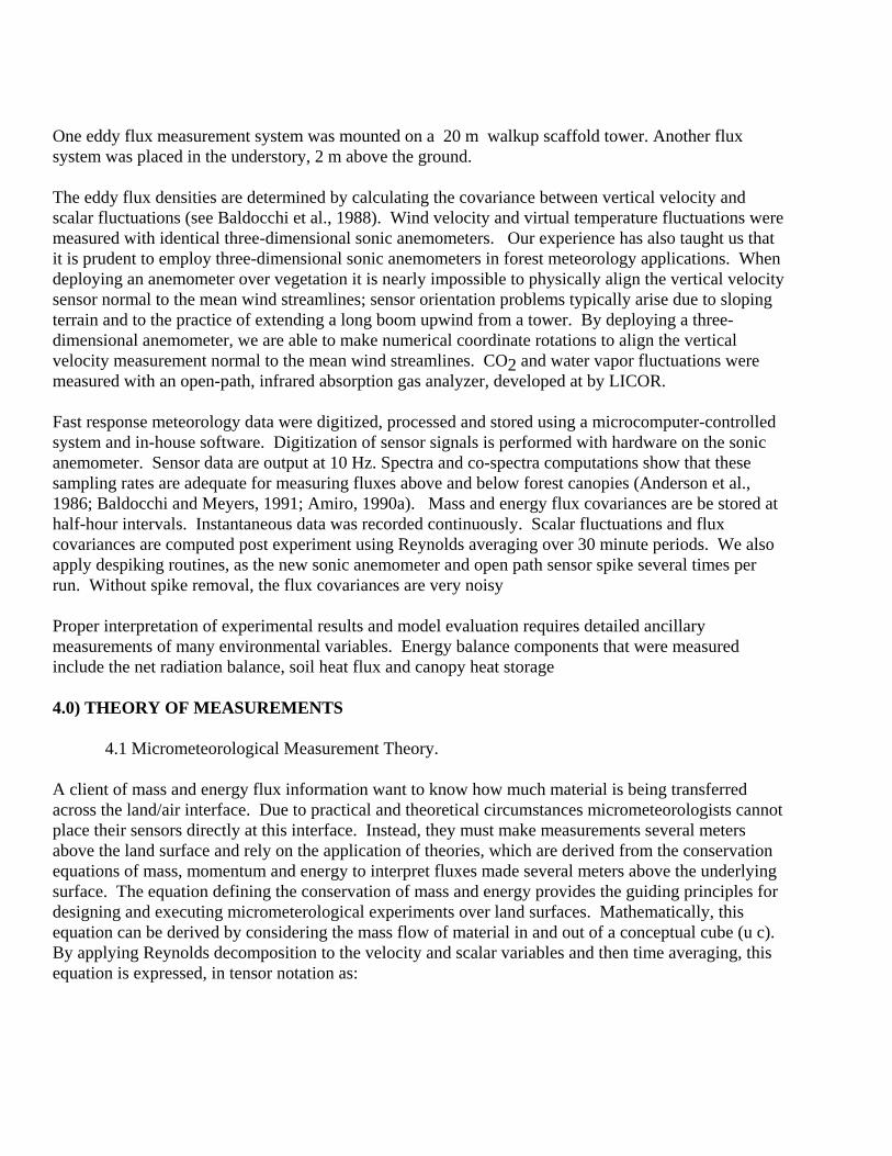
natural variability exceeds about +/-10%, so it is desirable to design a system with an error approaching this metric. Moore (1986) discusses transfer functions for sensor response time and separation distance. We preformed preliminary calculations of transfer function integrals. Corrections due to sensor time constants and separation are less than a few percent. Hence, we decided not to make transfer function to our flux measurements; our experimental design minimized the need for such corrections since we used an open path infrared gas analyzer and a sonic anemometer. Furthermore, these instruments were placed over a tall rough forest, so small distances in physical displacement have little impact on the measurement of scalar flux densities.

GrasslandVaira Ranch2 m tower, 3 m/s wind

f= nz/u

0.000001 0.00001 0.0001 0.001 0.01 0.1 1 10

Tra

nsfe

r Fu

ncti

on

0.0

0.2

0.4

0.6

0.8

1.0

1.2

1.4

1.6

1.8

2.0

w'T': 1.02w'q': 1.12w'u': 1.01w'c': 1.12

Figure 1 Transfer function of eddy fluxes for the current grassland configureation. Potential errors for moderate winds and stable conditions may reach 10% on the basis of Moore algorithms.

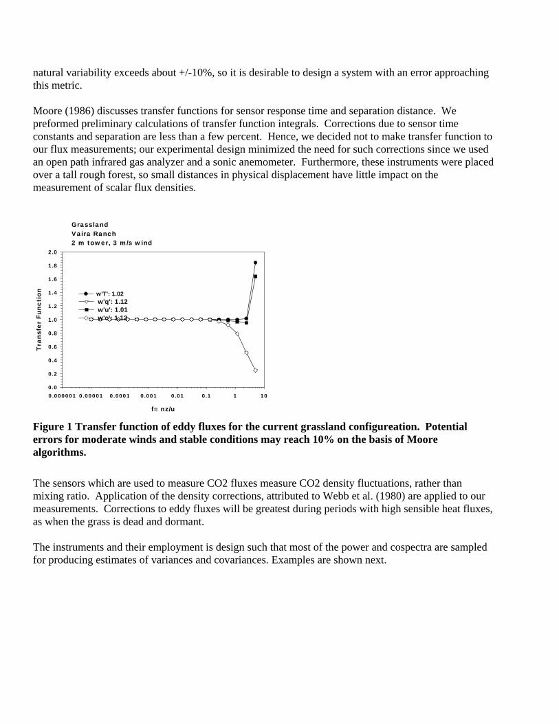
The sensors which are used to measure CO2 fluxes measure CO2 density fluctuations, rather than mixing ratio. Application of the density corrections, attributed to Webb et al. (1980) are applied to our measurements. Corrections to eddy fluxes will be greatest during periods with high sensible heat fluxes, as when the grass is dead and dormant. The instruments and their employment is design such that most of the power and cospectra are sampled for producing estimates of variances and covariances. Examples are shown next.

f/u

0.0001 0.001 0.01 0.1 1 10

nSxx

(n)/x

x

0.0001

0.001

0.01

0.1

1

wwcc

Figure 2 Power spectrum for vertical velocity and CO2 on savanna tower

f/u

0.0001 0.001 0.01 0.1 1 10

nSw

c(n)

/wc

0.0001

0.001

0.01

0.1

1

Tonzi Tower, D151

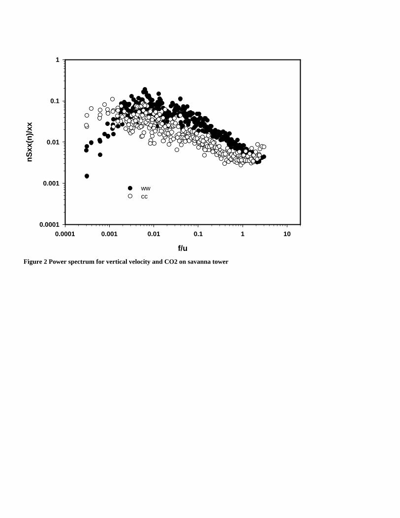
Figure 3 Co2 Co-spectrum over Tonzi ranch

5.0) EQUIPMENT - 5.1) Instrument Description. The experiment includes instrument setups for eddy covariance, meteorology and soil physical properties. The eddy Flux system involves measurements of turbulence, vertical, horizontal wind velocities and virtual temperature. The instruments include: Sonic anemometer: Gill Windmaster Pro, CO2 and water vapor concentrations: Licor-LI7500 CO2 Gashound, LI-800 Meteorological Variables PAR incoming: Kipp and Zonen PAR-Lite PAR reflected: Kipp and Zonen PAR lite Net radiometer: Kipp and Zonen, NR lite Pyranometer: Kipp and Zonen Pressure: Vaisala

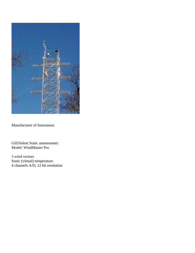
Temperature: Vaisala, HMP (sensor U3030042) Relative humidity: Vaisala, HMP Rain, Texas Electronics, tipping bucket, TE 5252mm (sensor LX 243734) Soil variables include Soil heat flux plates: Huseflux (3) Soil temperature: UCB probes at 2, 4,8,16 and 32 cm (3) Soil moisture: Theta probe ML2x, Delta-T Devices (5), 2 at 10 cm, 2 at 20 cm and 1 at surface Soil CO2: Vaisala at 2, 8 and 16 cm in the open and under a tree Eddy covariance flux measurements are made using a triple-axis wind master prof sonic anemometer and a Licor 7500 infrared absorption spectrometer. The sonic anemometer measured vertical (w) and horizontal (u,v) wind velocity and virtual air temperature (T). This anemometer model provides digital output at a rate of 10 Hz. The infrared absorption spectrometer measures water vapor and CO2 density fluctuations. The sensor responds to frequencies up to 10 Hz, has low noise and high sensitivity. The sensor is rugged and experiences little drift over several weeks of continuous operation. Soil heat flux density is measured by averaging the output of three soil heat flux plates (Huseflux). They are buried 0.01 m below the surface and were randomly placed within a few meters of the flux system. Soil temperature are measured with two multi-level thermocouple probes. Sensors are spaced logarithmically at 0.02, 0.04, 0.08, 0.16 and 0.32 m below the surface. Photosynthetically active photon flux density, solar radiation and the net radiation balance are measured above the grassland with a quantum sensor (Kipp and Zonen PAR lite), pyranometer (Kipp and Zonen) and a net radiometer (Kipp and Zonen), respectively. A LICOR line sensor (modelxxx) is used to measure light through the grass Air temperature and relative humidity are measured with appropriate sensors (Vaisala, model HMP-35A). Static pressure is measured with a Vaisala model PTB101B sensor. It operates on a 600 to 1060 mb range over 2.5 volts. Ancillary meteorological and soil physics data are acquired and logged on a Campbell CR-23x and CR-10x data loggers. Half-hour averages were stored on a computer, to coincide with the flux measurements. CO2 concentration profiles were originally measured with the LICOR 7500. We now have a dedicated profile system using the LI-800 that is zeroed and calibrated 2 times per day. Pressure through the cell is controlled to 1 part per 1000 with a pressure controller. Temperature of the cell is maintained near 50 C and is measured with an independent thermocouple.

A radiation tram system was installed in the forest understory during the spring of 2006. A net radiometer and up and down facing quantum sensor will traverse back and forth along a 30 m transect. - 5.1.1 Principles of Operation. Sonic Anemometer: Three-dimensional orthogonal wind velocities (u,v and w) and virtual temperature (Tv) were measured with a sonic anemometer (Wind Master Pro). The pathlength between transducers was 0.15 m. The sensor software corrected for transducer shadowing effects (see Kaimal et al. 1990). Virtual temperature heat flux was converted to sensible heat flux using algorithms described by Kaimal and Gaynor (1991). Infrared Absorption Spectrometer: Water vapor and CO2 concentrations were measured with an open-path infrared absorption spectrometer. Soil Heat Flux Transducer: An encapsulated thermopile yields a voltage output proportional to the temperature difference across the top and bottom surfaces. The device has been calibrated in terms of heat flux through transducer corresponding to the observed temperature difference. Instrument Measurement Geometry. The eddy flux measurement system was placed at 2 m above the ground. The Licor 7500 was 0.15 m beside the sensor Power: solar panels

Siemens SP75 panels in parallel with Morningstar 30 regulator and 6 12 vdc batteries. The forest floor system draw is 2.1 amps. The tower system draws about 4.3 amps. Six panels run the floor system and the tower systems.

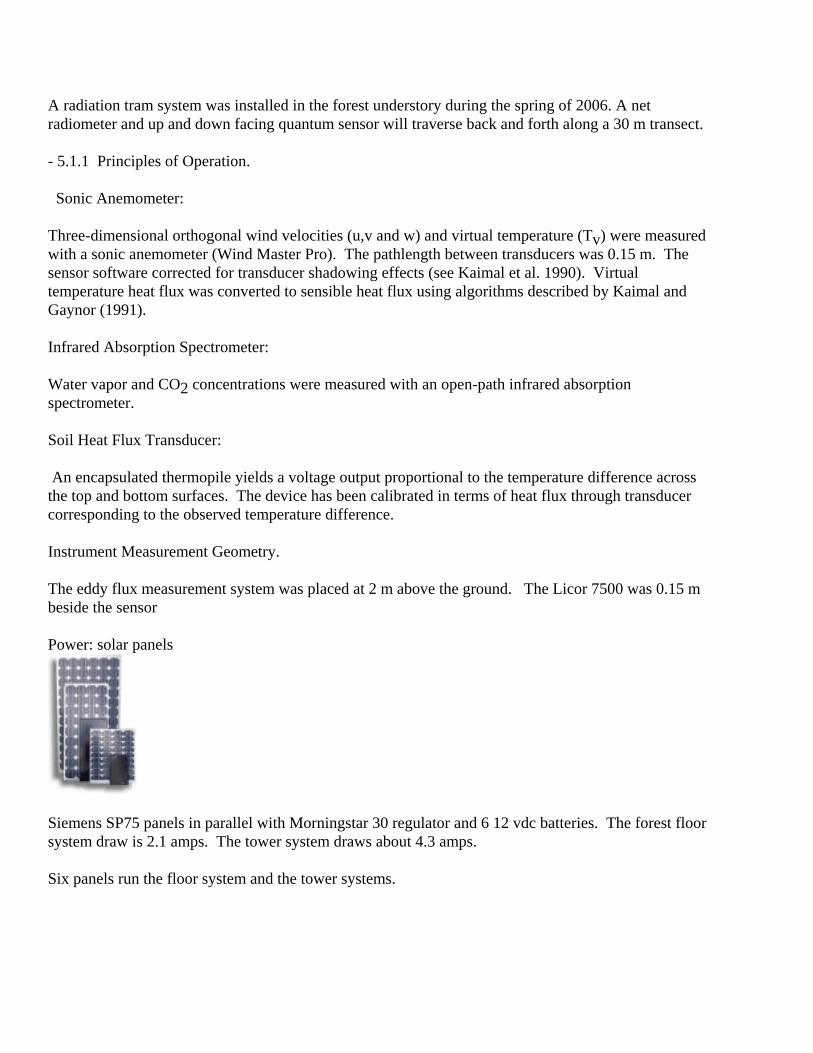
Manufacturer of Instrument. Gill/Solent Sonic anemometer: Model: WindMaster Pro 3 wind vectors Sonic (virtual) temperature 4 channels A/D, 12 bit resolution

Soil heat transducer: HuseFlux

Figure 4

Net Radiometer:

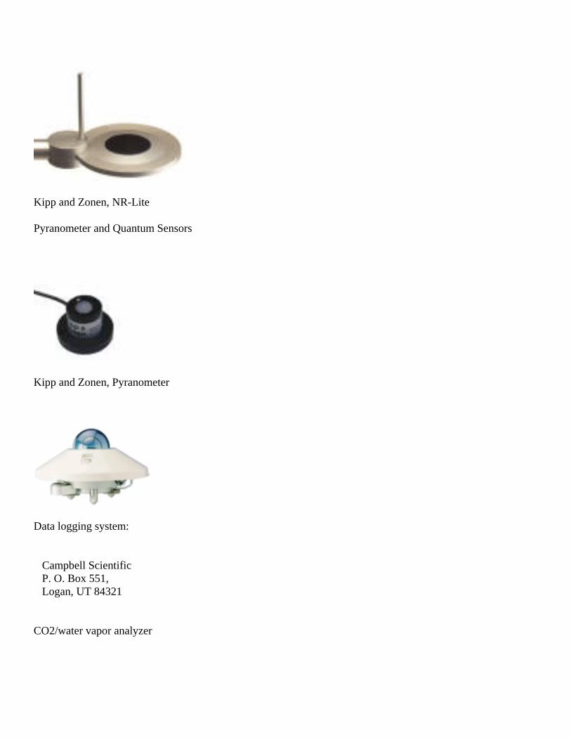
Kipp and Zonen, NR-Lite Pyranometer and Quantum Sensors

Kipp and Zonen, Pyranometer

Data logging system: Campbell Scientific P. O. Box 551, Logan, UT 84321 CO2/water vapor analyzer

LI 7500 LICOR 4421 Superior St Lincoln, NE

Temperature and humidity Vaisala

Pressure Sensor Static Vaisala Physiology LI 6400 Licor

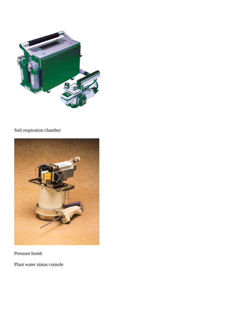
Soil respiration chamber

Pressure bomb Plant water status console

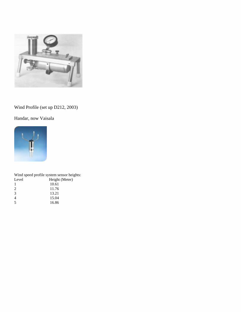
Wind Profile (set up D212, 2003) Handar, now Vaisala

Wind speed profile system sensor heights: Level Height (Meter) 1 10.61 2 11.76 3 13.21 4 15.04 5 16.86

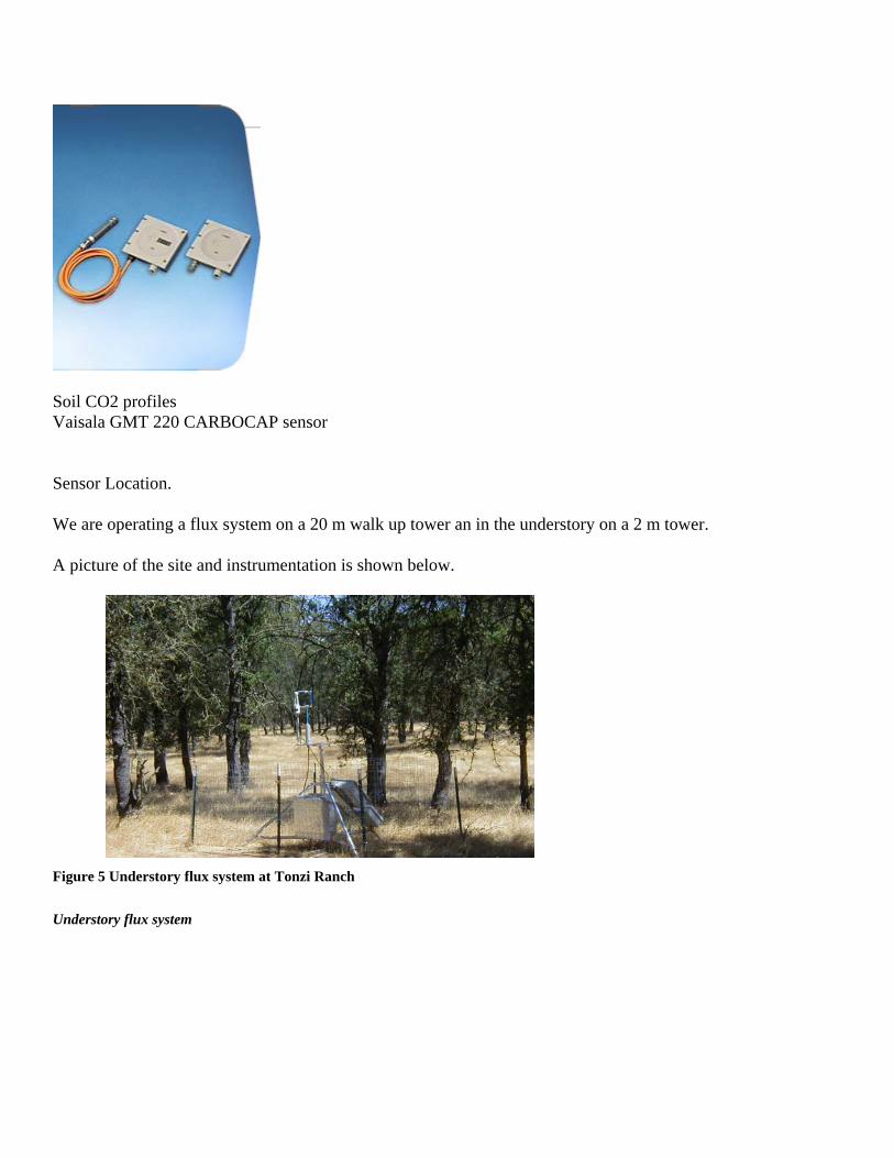
Soil CO2 profiles Vaisala GMT 220 CARBOCAP sensor Sensor Location. We are operating a flux system on a 20 m walk up tower an in the understory on a 2 m tower. A picture of the site and instrumentation is shown below.

Figure 5 Understory flux system at Tonzi Ranch

Understory flux system

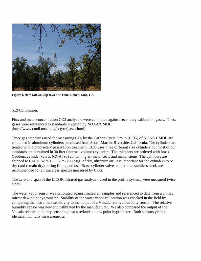
Figure 6 20 m tall walkup tower at Tonzi Ranch, Ione, CA

5.2) Calibration. Flux and mean concentration CO2 analyzers were calibrated against secondary calibration gases. These gases were referenced to standards prepared by NOAA/CMDL (http://www.cmdl.noaa.gov/ccg/refgases.html) Trace gas standards used for measuring CO2 by the Carbon Cycle Group (CCG) of NOAA CMDL are contained in aluminum cylinders purchased from Scott- Marrin, Riverside, California. The cylinders are treated with a proprietary passivation treatment. CCG uses three different size cylinders but most of our standards are contained in 30 liter (internal volume) cylinders. The cylinders are ordered with brass Ceodeux cylinder valves (CGA590) containing all-metal seats and nickel stems. The cylinders are shipped to CMDL with 1380 kPa (200 psig) of dry, ultrapure air. It is important for the cylinders to be dry (and remain dry) during filling and use. Brass cylinder valves rather than stainless steel, are recommended for all trace gas species measured by CCG. The zero and span of the LICOR infrared gas analyzer, used in the profile system, were measured twice a day. The water vapor sensor was calibrated against mixed air samples and referenced to data from a chilled mirror dew point hygrometer. Stability of the water vapor calibration was checked in the field by comparing the instrument sensitivity to the output of a Vaisala relative humidity sensor. The relative humidity sensor was new and calibrated by the manufacturer. We also compared the output of the Vaisala relative humidity sensor against a redundant dew point hygrometer. Both sensors yielded identical humidity measurements.

Radiation sensors are calibrated against a set of laboratory standards about once per year. We periodically send the sonic anemometers, Licor gas analyzers and Vaisala CO2 and T/RH probes back to the manufacturers for lab calibration and maintenance. - 5.2.1) Specifications. Calibration factors. Sonic anemometer: supplied by manufacturer. 1.0 m s-1/V with sonic pathlength 0.15 m. Carbon dioxide: Water vapor density fluctuations: varies with vapor density Soil heat transducer: net radiation: quantum flux density: 180 µmol m-2 s-1 mv-1 Pressure: 0.184 mb/mv - 5.2.1.1) Tolerance. Precision or sensitivity estimates: Solar and net radiation: 1 W m-2. Air temperature fluctuations: 0.1 K. Vertical wind velocity fluctuations: 0.01 m s-1. Surface radiative temperature; 0.1 K. Other Calibration Information. CO2 gases were originally referenced to NIST standards. We have depleted those gases and recently purchased standards from Dr. Pieter Tans, CMDL/NOAA lab.

National Oceanic and Atmospheric Administration Climate Monitoring and Diagnostics Lab Carbon Cycle Greenhouse Gases group R-E-CG1 325 Broadway Boulder, CO. 80303 E-Mail dkitzis@cmdl.noaa.gov Phone 303-497-6675 Fax 303-497-6750

http://www.cmdl.noaa.gov/ccgg/refgases/airstandard.html

References The manometric calibration system is described in more detail in Zhao, C., P.P. Tans and K.W. Thoning, A high precision manometric system for absolute calibrations of CO2 in dry air. Journal of Geophysical Research102(D5):5885-5894 March 20, 1997

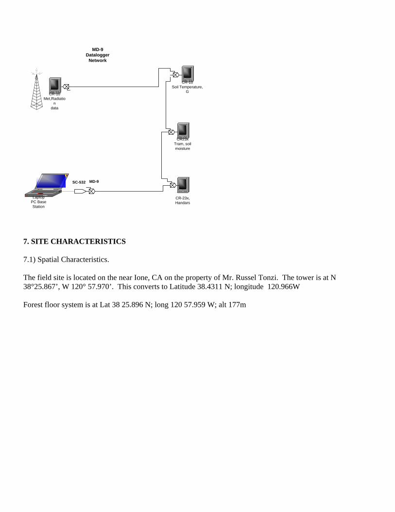
6.0) PROCEDURE 6.1) Data Acquisition Methods. We use a system of daisy changed CR10x and CR23x data loggers, connected via coax cable and Md-9s to log and store the meteorological and soil data. These are tied to a pc which runs the pc208 software. The data are written to disk each 30 min. Once each day the data files are renamed with information on the logger, year and day. For example, CR23x2 stores data to CR23x2.dat. At midnight this file becomes TZ2_yrday.23x, or file CR10x4 stored data as CR10x4.dat. At midnight that file becomes TZ4_yrday.10x.

LaptopPC BaseStation

CR-10Met,Radiatio

ndata

CR23xTram, soilmoisture

CR-10Soil Temperature,

G

CR-23x,Handars

MD-9Datalogger

Network

SC-532 MD-9

7. SITE CHARACTERISTICS 7.1) Spatial Characteristics. The field site is located on the near Ione, CA on the property of Mr. Russel Tonzi. The tower is at N 38°25.867’, W 120° 57.970’. This converts to Latitude 38.4311 N; longitude 120.966W Forest floor system is at Lat 38 25.896 N; long 120 57.959 W; alt 177m

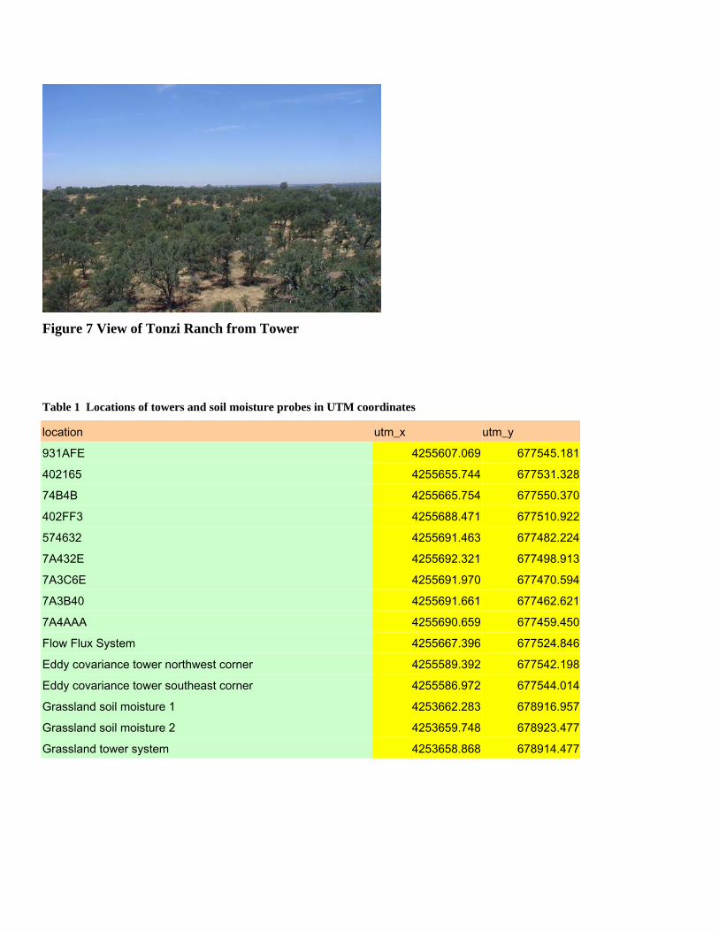
Figure 7 View of Tonzi Ranch from Tower

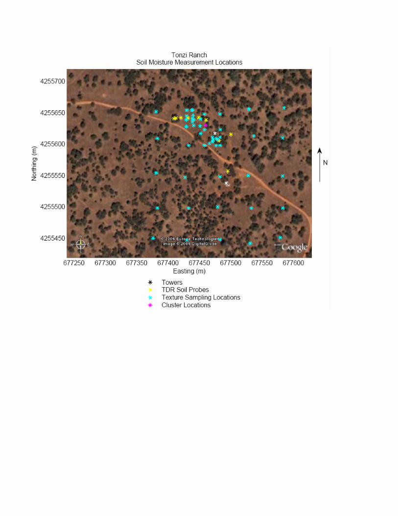
Table 1 Locations of towers and soil moisture probes in UTM coordinates

location utm_x utm_y 931AFE 4255607.069 677545.181

402165 4255655.744 677531.328

74B4B 4255665.754 677550.370

402FF3 4255688.471 677510.922

574632 4255691.463 677482.224

7A432E 4255692.321 677498.913

7A3C6E 4255691.970 677470.594

7A3B40 4255691.661 677462.621

7A4AAA 4255690.659 677459.450

Flow Flux System 4255667.396 677524.846

Eddy covariance tower northwest corner 4255589.392 677542.198

Eddy covariance tower southeast corner 4255586.972 677544.014

Grassland soil moisture 1 4253662.283 678916.957

Grassland soil moisture 2 4253659.748 678923.477

Grassland tower system 4253658.868 678914.477

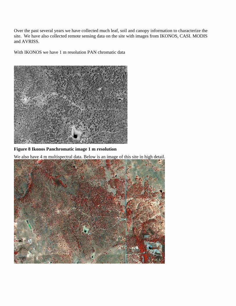
Over the past several years we have collected much leaf, soil and canopy information to characterize the site. We have also collected remote sensing data on the site with images from IKONOS, CASI. MODIS and AVRISS. With IKONOS we have 1 m resolution PAN chromatic data

Figure 8 Ikonos Panchromatic image 1 m resolution

We also have 4 m multispectral data. Below is an image of this site in high detail.

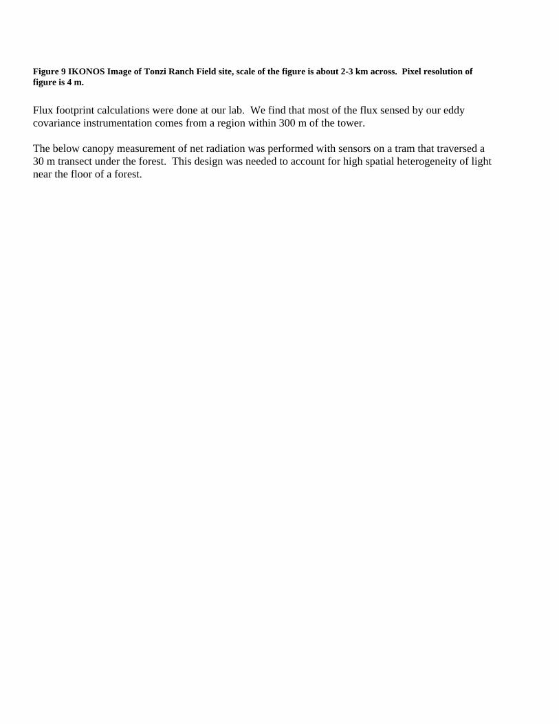
Figure 9 IKONOS Image of Tonzi Ranch Field site, scale of the figure is about 2-3 km across. Pixel resolution of figure is 4 m.

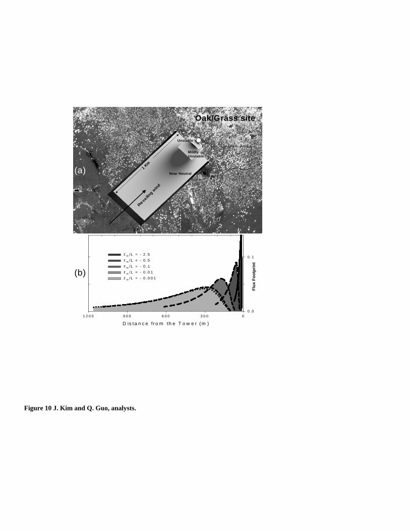
Flux footprint calculations were done at our lab. We find that most of the flux sensed by our eddy covariance instrumentation comes from a region within 300 m of the tower. The below canopy measurement of net radiation was performed with sensors on a tram that traversed a 30 m transect under the forest. This design was needed to account for high spatial heterogeneity of light near the floor of a forest.

1 Km

Preva

iling w

ind

Unstable

MildlyUnstable

Near Neutral

Oak/Grass site

D is ta n c e f r o m th e T o w e r ( m )03 0 06 0 09 0 01 2 0 0

Flux

Foo

tprin

t

0 .0

0 .1z m /L = - 2 .5z m /L = - 0 .5z m /L = - 0 .1z m /L = - 0 .0 1z m /L = - 0 .0 0 1

(a)

(b)

Figure 10 J. Kim and Q. Guo, analysts.

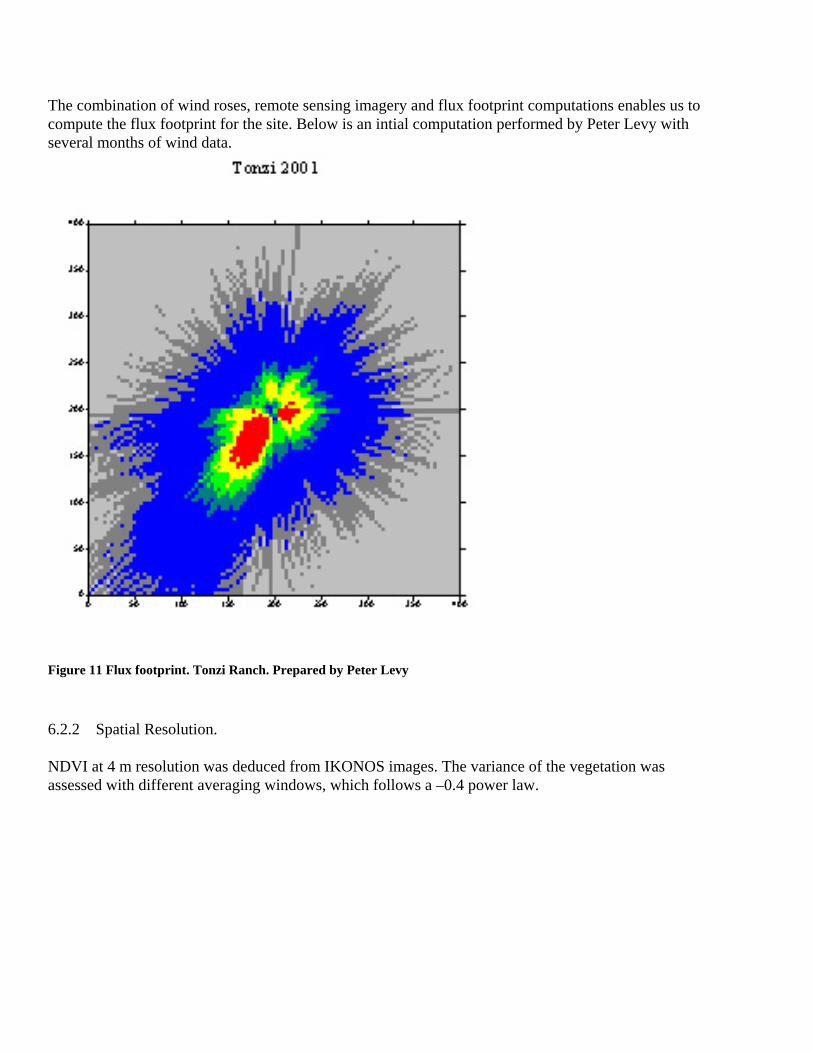
The combination of wind roses, remote sensing imagery and flux footprint computations enables us to compute the flux footprint for the site. Below is an intial computation performed by Peter Levy with several months of wind data.

Figure 11 Flux footprint. Tonzi Ranch. Prepared by Peter Levy

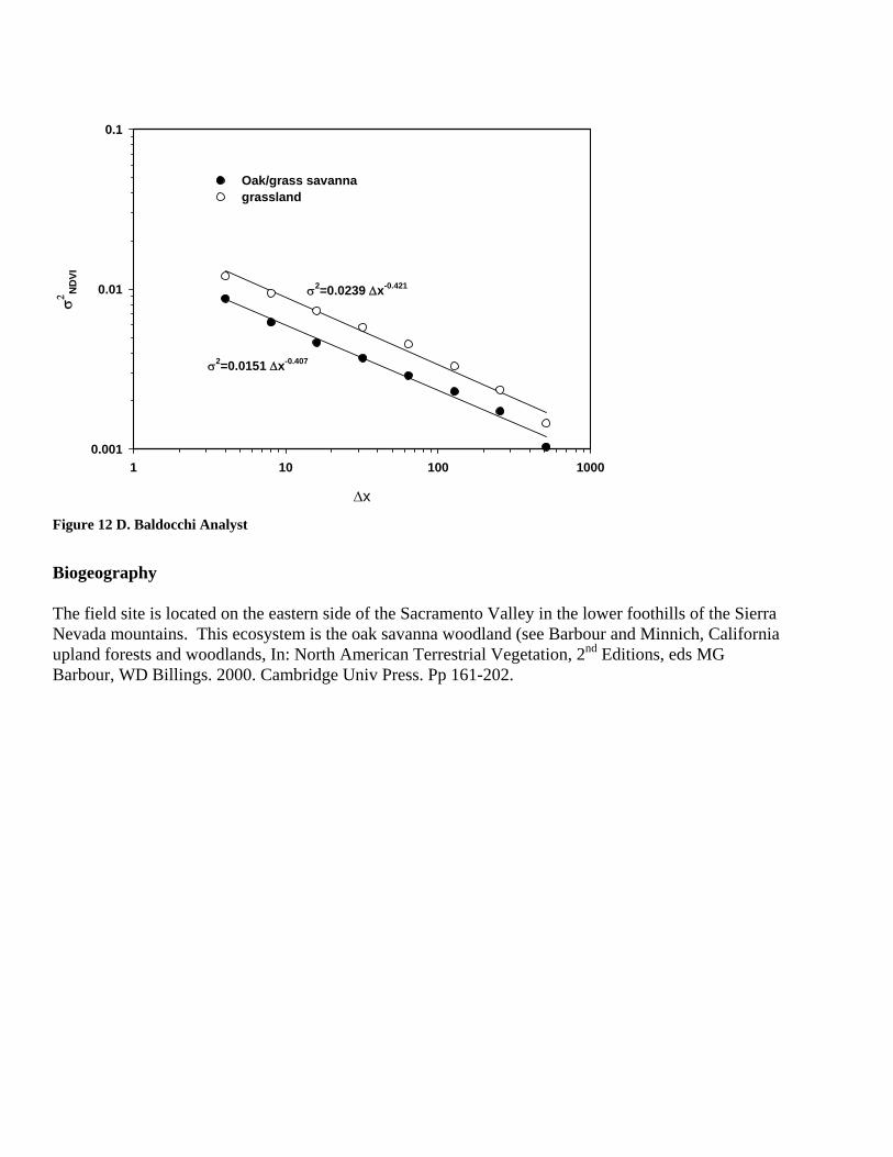
6.2.2 Spatial Resolution. NDVI at 4 m resolution was deduced from IKONOS images. The variance of the vegetation was assessed with different averaging windows, which follows a –0.4 power law.

∆x

1 10 100 1000

σ2 ND

VI

0.001

0.01

0.1

Oak/grass savannagrassland

σ2=0.0239 ∆x-0.421

σ2=0.0151 ∆x-0.407

Figure 12 D. Baldocchi Analyst Biogeography The field site is located on the eastern side of the Sacramento Valley in the lower foothills of the Sierra Nevada mountains. This ecosystem is the oak savanna woodland (see Barbour and Minnich, California upland forests and woodlands, In: North American Terrestrial Vegetation, 2nd Editions, eds MG Barbour, WD Billings. 2000. Cambridge Univ Press. Pp 161-202.

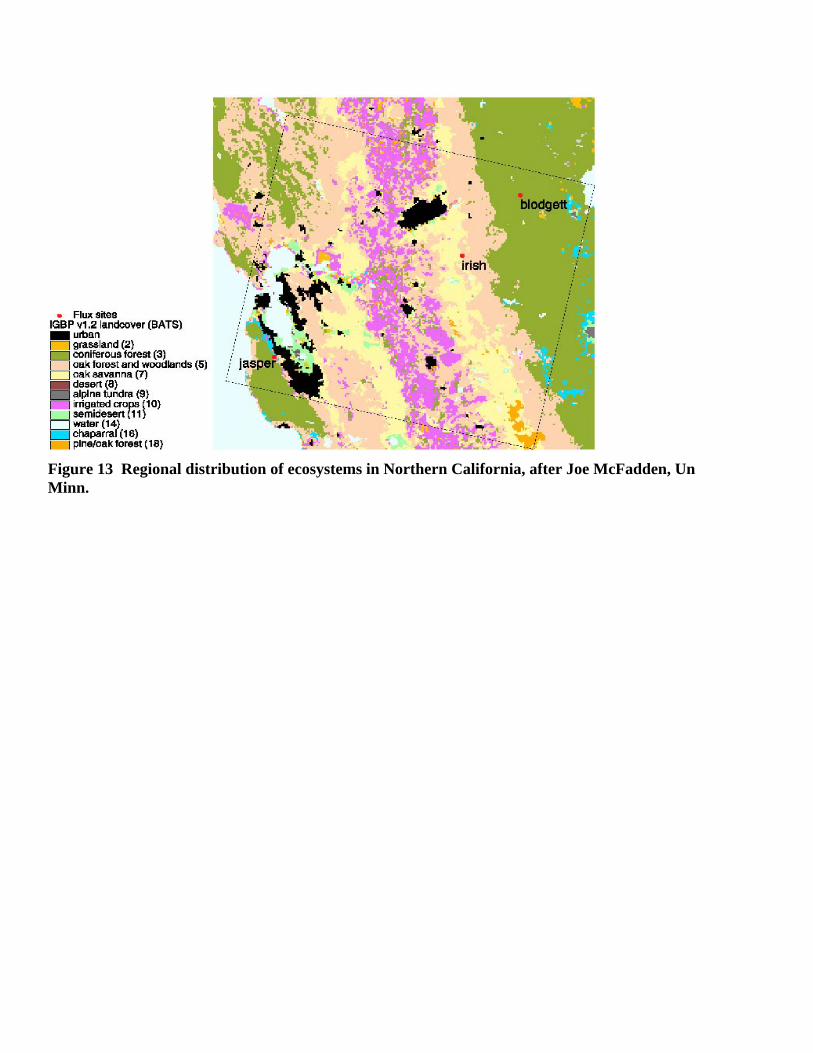
Figure 13 Regional distribution of ecosystems in Northern California, after Joe McFadden, Un Minn.

-124 -123 -122 -121 -120 -119 -118 -117 -116 -115Longitude

33

34

35

36

37

38

39

40

41

42

Latit

ude

Quercus douglasii Range

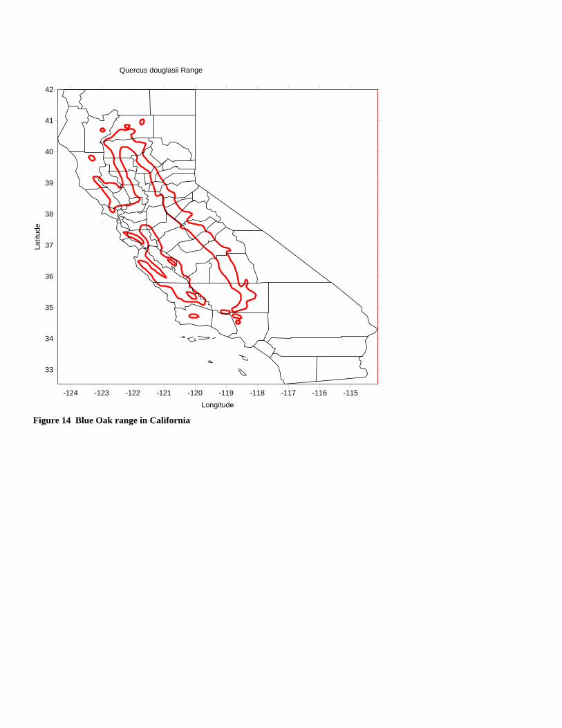
Figure 14 Blue Oak range in California

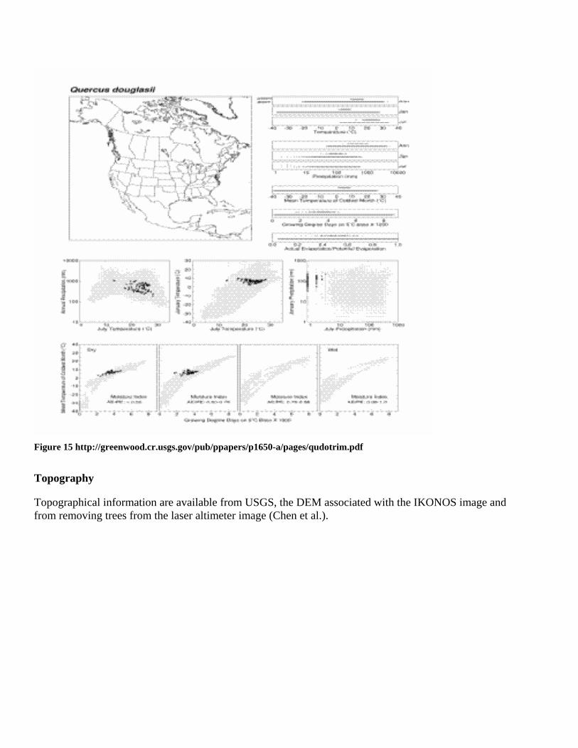
Figure 15 http://greenwood.cr.usgs.gov/pub/ppapers/p1650-a/pages/qudotrim.pdf Topography Topographical information are available from USGS, the DEM associated with the IKONOS image and from removing trees from the laser altimeter image (Chen et al.).

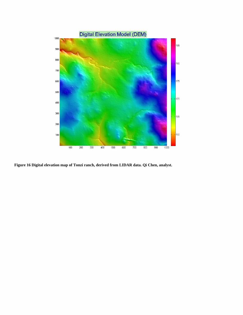
Figure 16 Digital elevation map of Tonzi ranch, derived from LIDAR data. Qi Chen, analyst.

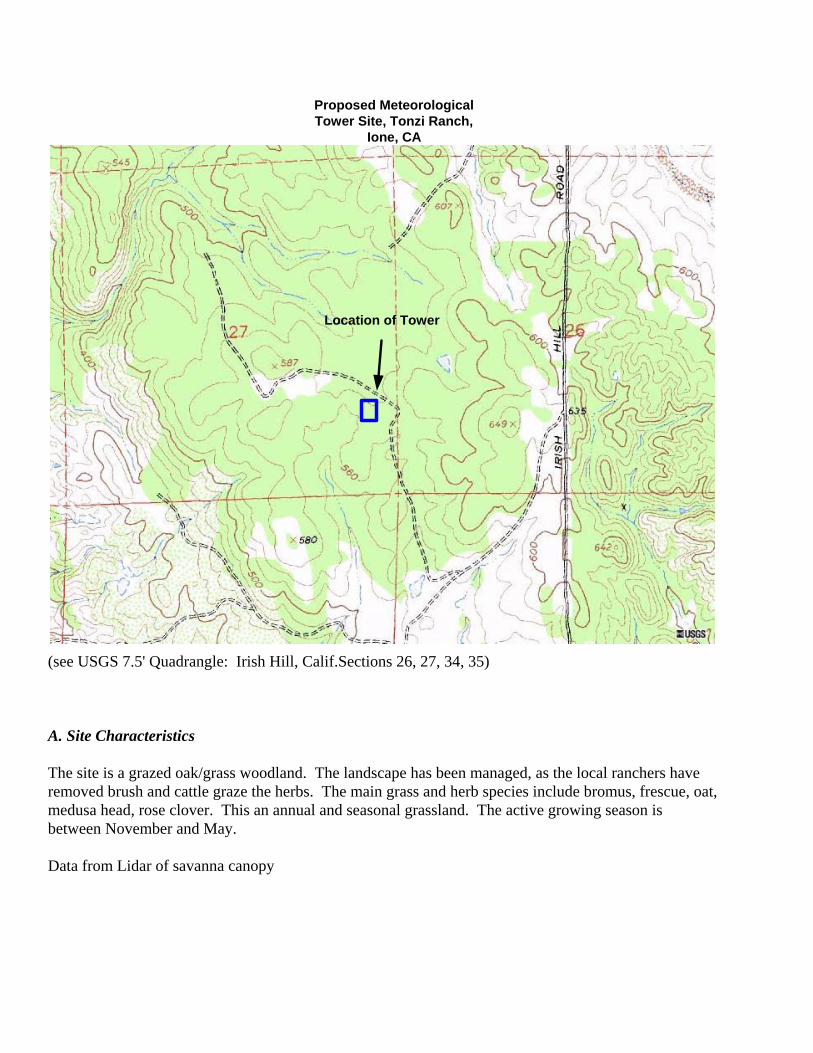
Location of Tower

Proposed MeteorologicalTower Site, Tonzi Ranch,

Ione, CA

(see USGS 7.5' Quadrangle: Irish Hill, Calif.Sections 26, 27, 34, 35) A. Site Characteristics

The site is a grazed oak/grass woodland. The landscape has been managed, as the local ranchers have removed brush and cattle graze the herbs. The main grass and herb species include bromus, frescue, oat, medusa head, rose clover. This an annual and seasonal grassland. The active growing season is between November and May. Data from Lidar of savanna canopy

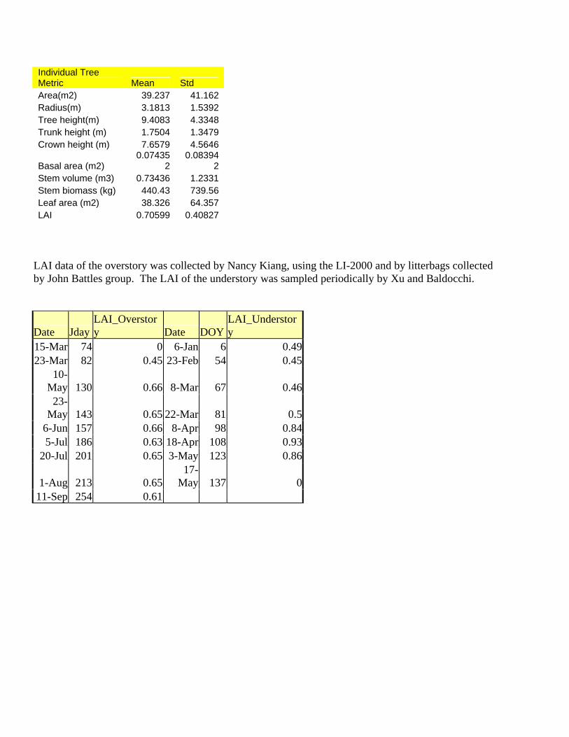
Individual Tree Metric Mean Std Area(m2) 39.237 41.162 Radius(m) 3.1813 1.5392 Tree height(m) 9.4083 4.3348 Trunk height (m) 1.7504 1.3479 Crown height (m) 7.6579 4.5646

Basal area (m2) 0.07435

2 0.08394

2 Stem volume (m3) 0.73436 1.2331 Stem biomass (kg) 440.43 739.56 Leaf area (m2) 38.326 64.357 LAI 0.70599 0.40827

LAI data of the overstory was collected by Nancy Kiang, using the LI-2000 and by litterbags collected by John Battles group. The LAI of the understory was sampled periodically by Xu and Baldocchi.

Date Jday LAI_Overstory Date DOY

LAI_Understory

15-Mar 74 0 6-Jan 6 0.4923-Mar 82 0.45 23-Feb 54 0.45

10-May 130 0.66 8-Mar 67 0.4623-

May 143 0.65 22-Mar 81 0.56-Jun 157 0.66 8-Apr 98 0.845-Jul 186 0.63 18-Apr 108 0.93

20-Jul 201 0.65 3-May 123 0.86

1-Aug 213 0.65 17-

May 137 011-Sep 254 0.61

Oak/grass savanna

DOY

0 100 200 300

LAI

0.0

0.5

1.0

1.5

2.02001

Understorey grass

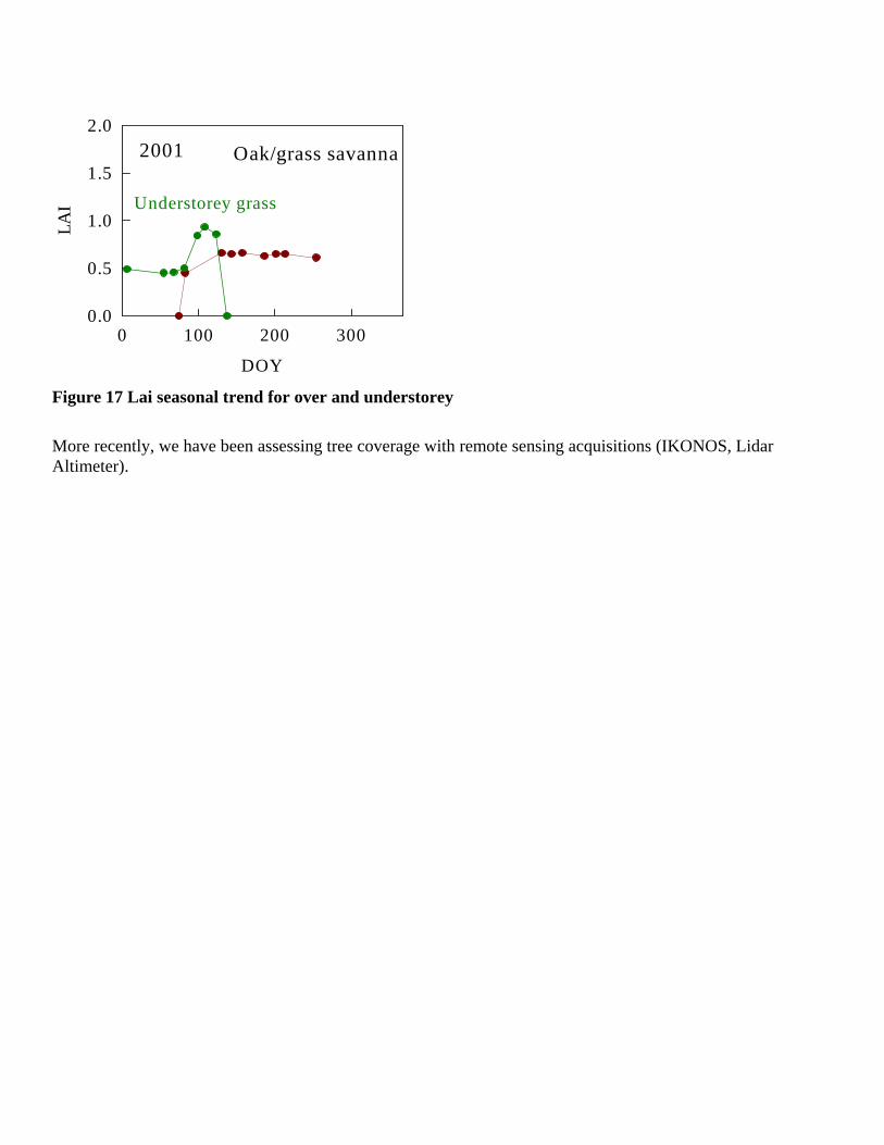
Figure 17 Lai seasonal trend for over and understorey

More recently, we have been assessing tree coverage with remote sensing acquisitions (IKONOS, Lidar Altimeter).

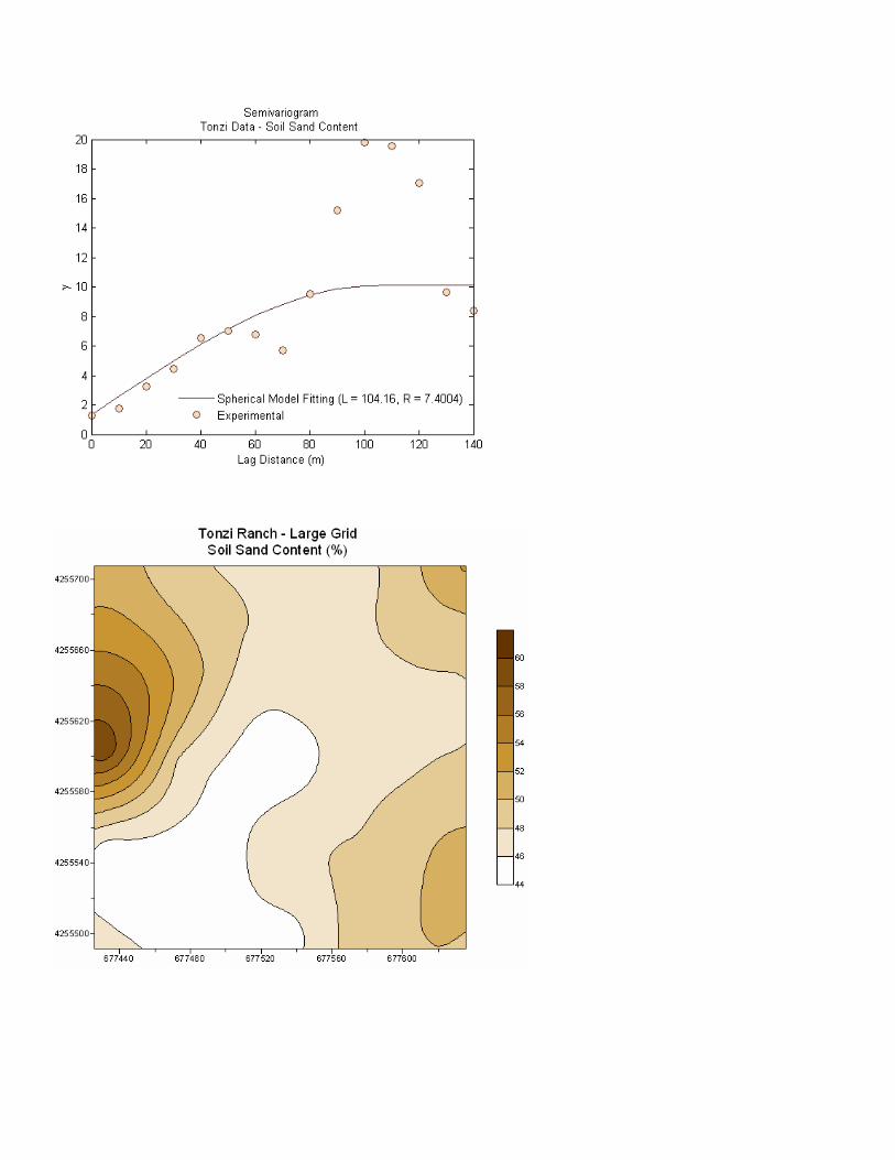
Lag Distance (m)

0 10 20 30 40 50

ND

VI V

ario

gram

0.000

0.002

0.004

0.006

0.008

0.010

Tonzi Ranch, IKONOS data, computed by P.Levy

Figure 18 Lag Correlation of NDVI from IKONOS Image. Produces information on the scale of gaps in the canopy. They tend to be less than 10 m.

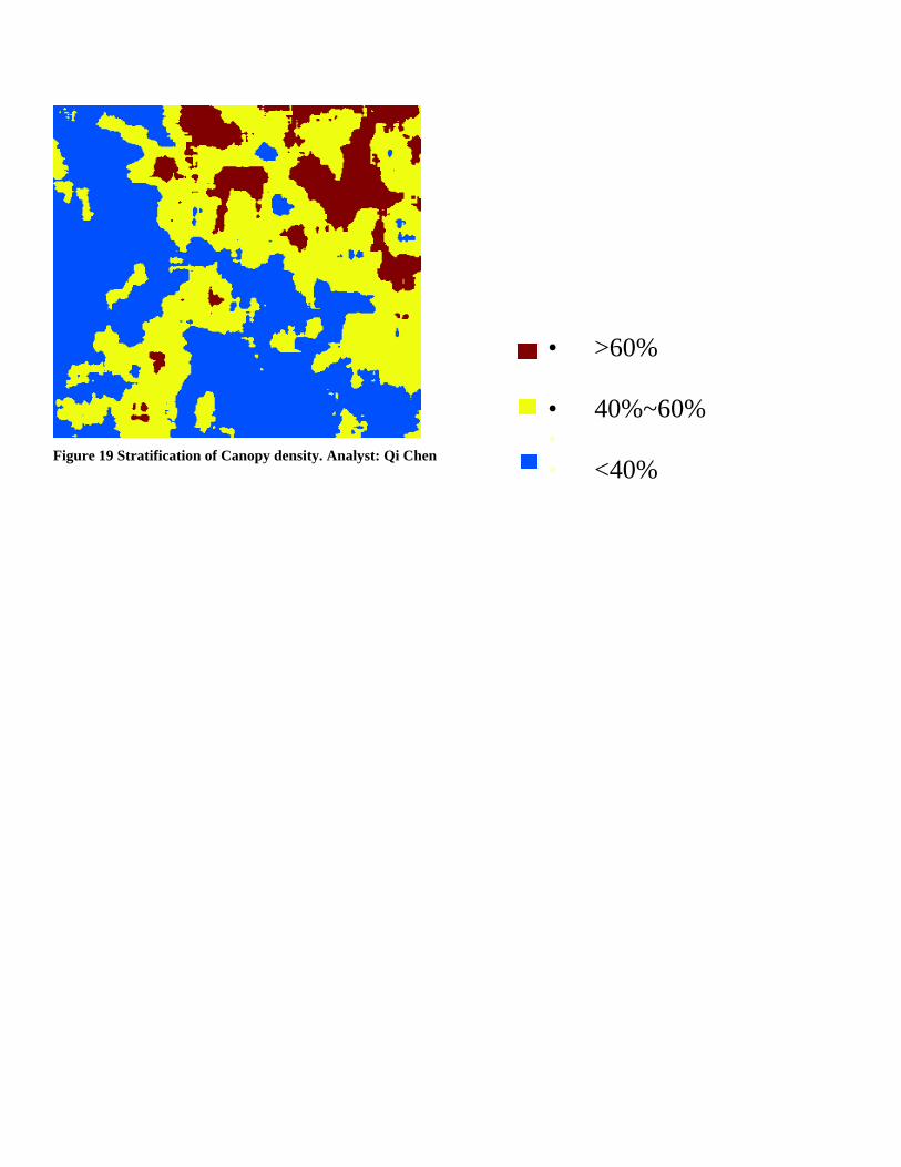
• >60%

• 40%~60% • • <40%

Figure 19 Stratification of Canopy density. Analyst: Qi Chen

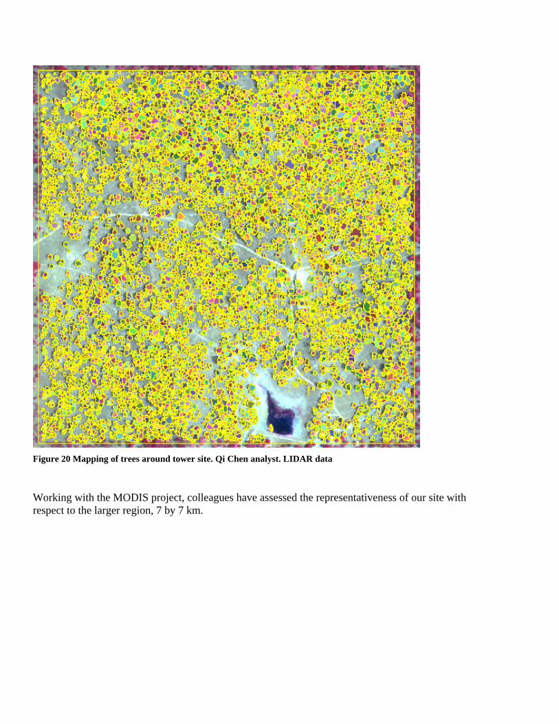
Figure 20 Mapping of trees around tower site. Qi Chen analyst. LIDAR data

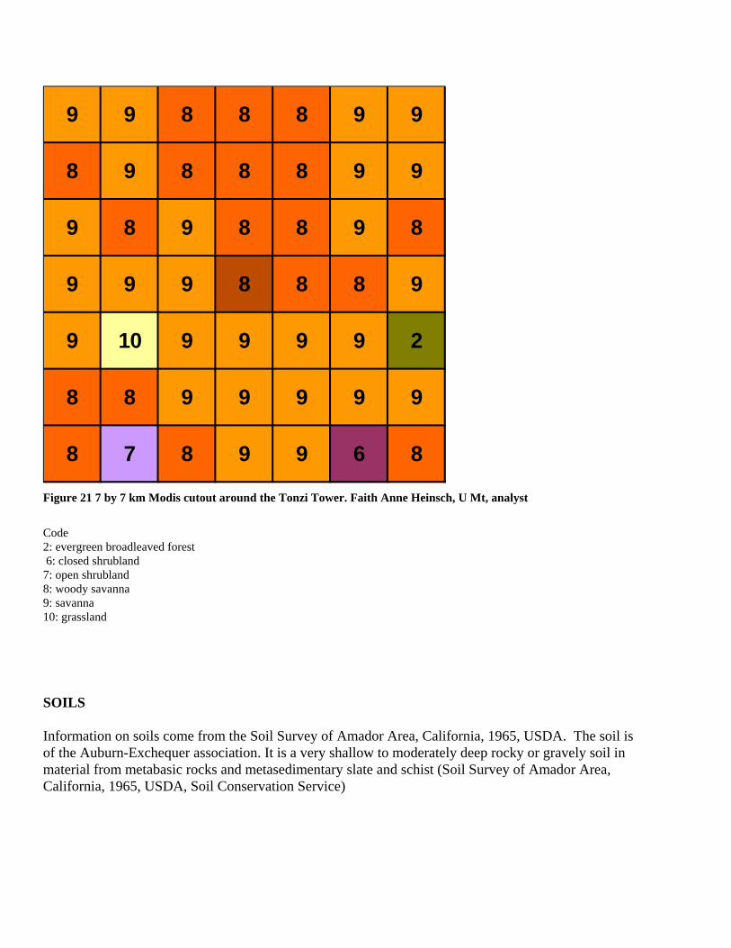
Working with the MODIS project, colleagues have assessed the representativeness of our site with respect to the larger region, 7 by 7 km.

9 9 8 8 8 9 9

8 9 8 8 8 9 9

9 8 9 8 8 9 8

9 9 9 8 8 8 9

9 10 9 9 9 9 2

8 8 9 9 9 9 9

8 7 8 9 9 6 8

Figure 21 7 by 7 km Modis cutout around the Tonzi Tower. Faith Anne Heinsch, U Mt, analyst

Code 2: evergreen broadleaved forest 6: closed shrubland 7: open shrubland 8: woody savanna 9: savanna 10: grassland SOILS Information on soils come from the Soil Survey of Amador Area, California, 1965, USDA. The soil is of the Auburn-Exchequer association. It is a very shallow to moderately deep rocky or gravely soil in material from metabasic rocks and metasedimentary slate and schist (Soil Survey of Amador Area, California, 1965, USDA, Soil Conservation Service)

Classified as AsD, Auburn extremely rocky silt loam, 3 to 31 percent slopes. The profile is: *0-9 inches, strong brown silt loam, Massive. Hard when dry, friable when wet slightly acid *9-14 inches yellowish red silt loam. Massive. Hard when dry, friable when wet, slightly acid. *14 inches plus, weathered, very pale brown AUBURN SERIES The Auburn series consists of shallow to moderately deep, well drained soils formed in material weathered from amphibolite schist. Auburn soils are on foothills and have slopes of 2 to 75 percent. The mean annual precipitation is about 24 inches and the mean annual temperature is about 60 degrees F. TAXONOMIC CLASS: Loamy, mixed, superactive, thermic Lithic Haploxerepts AUBURN Date SC Updated: 08-MAR-01 MO Responsible: 2 (DAVIS, CALIFORNIA) State Type Location: CA Series Status: E Classification Subgroup Soil Order: INCEPTISOLS Suborder: XEREPTS Great Group: HAPLOXEREPTS Subgroup Modifier: LITHIC Family Particle Size: LOAMY Particle Size Modifier: Mineralogy: MIXED CEC Activity: SUPERACTIVE Reaction: Soil Temperature: THERMIC Other: TYPICAL PEDON: Auburn silt loam - on an east facing slope of 10 percent under annual grass, oak and digger pine at 620 feet elevation. (Colors are for dry soil unless otherwise stated. When described on March 27, 1959, the soil was dry throughout.)

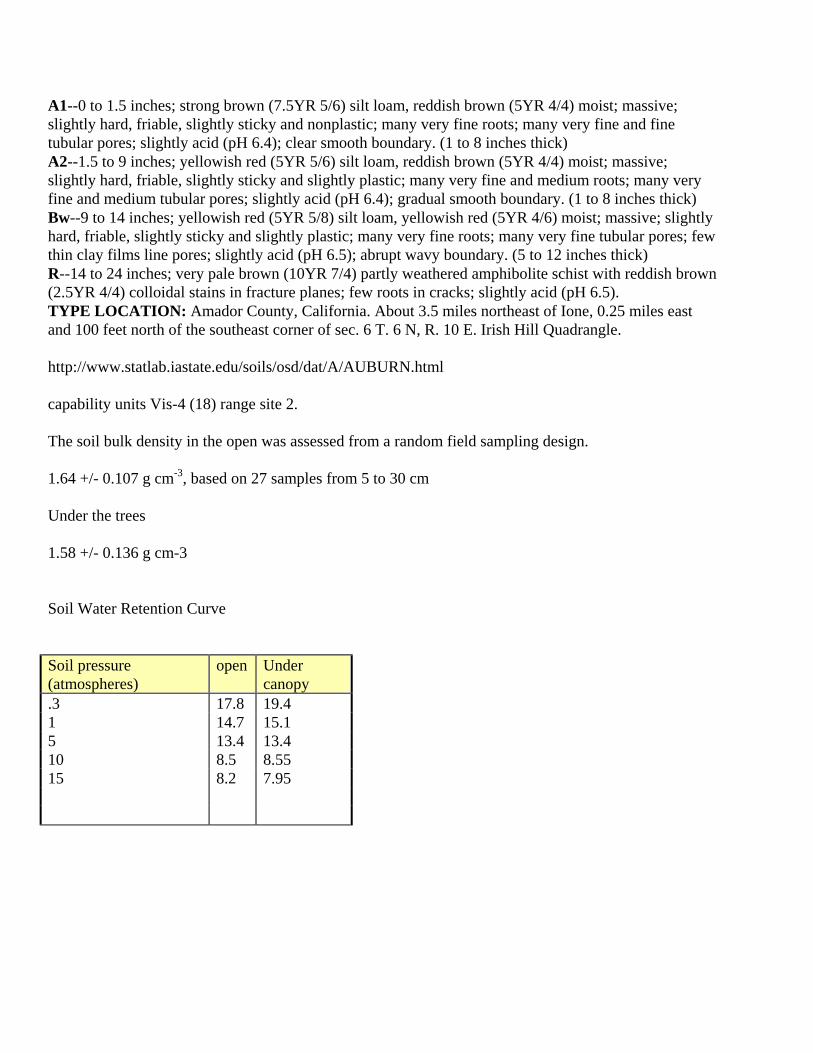
A1--0 to 1.5 inches; strong brown (7.5YR 5/6) silt loam, reddish brown (5YR 4/4) moist; massive; slightly hard, friable, slightly sticky and nonplastic; many very fine roots; many very fine and fine tubular pores; slightly acid (pH 6.4); clear smooth boundary. (1 to 8 inches thick) A2--1.5 to 9 inches; yellowish red (5YR 5/6) silt loam, reddish brown (5YR 4/4) moist; massive; slightly hard, friable, slightly sticky and slightly plastic; many very fine and medium roots; many very fine and medium tubular pores; slightly acid (pH 6.4); gradual smooth boundary. (1 to 8 inches thick) Bw--9 to 14 inches; yellowish red (5YR 5/8) silt loam, yellowish red (5YR 4/6) moist; massive; slightly hard, friable, slightly sticky and slightly plastic; many very fine roots; many very fine tubular pores; few thin clay films line pores; slightly acid (pH 6.5); abrupt wavy boundary. (5 to 12 inches thick) R--14 to 24 inches; very pale brown (10YR 7/4) partly weathered amphibolite schist with reddish brown (2.5YR 4/4) colloidal stains in fracture planes; few roots in cracks; slightly acid (pH 6.5). TYPE LOCATION: Amador County, California. About 3.5 miles northeast of Ione, 0.25 miles east and 100 feet north of the southeast corner of sec. 6 T. 6 N, R. 10 E. Irish Hill Quadrangle. http://www.statlab.iastate.edu/soils/osd/dat/A/AUBURN.html capability units Vis-4 (18) range site 2. The soil bulk density in the open was assessed from a random field sampling design. 1.64 +/- 0.107 g cm-3, based on 27 samples from 5 to 30 cm Under the trees 1.58 +/- 0.136 g cm-3 Soil Water Retention Curve Soil pressure (atmospheres)

open Under canopy

.3 17.8 19.4 1 14.7 15.1 5 13.4 13.4 10 8.5 8.55 15 8.2 7.95

Soil moisture release curve

Gravimetric soil water content (%) 0 10 20 30 40

Wat

er p

oten

tial (

-bar

)

0

20

40

60

80

100

120

140

160

Data from dew point Data from DANR

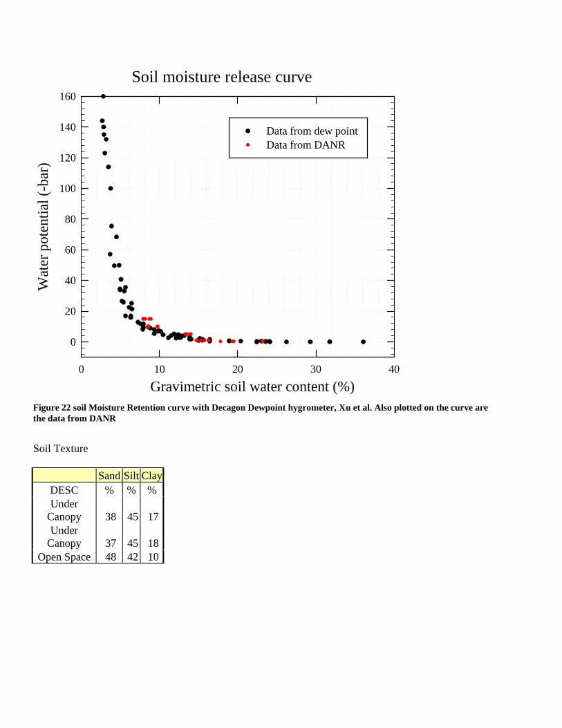
Figure 22 soil Moisture Retention curve with Decagon Dewpoint hygrometer, Xu et al. Also plotted on the curve are the data from DANR Soil Texture

Sand Silt Clay DESC % % % Under

Canopy 38 45 17 Under

Canopy 37 45 18 Open Space 48 42 10

Figure 23 Geological soils map for the Ione, CA area near the Tonzi and Vaira ranches

Soil thermal conductivity was determined with the amplitude method documented in Verhoef et al. AT this site it varies with time and soil moisture

Soil thermal conductivity, Vaira 2002 data

θv(m3 m-3)

0.0 0.1 0.2 0.3 0.4 0.5

KT

(W m

-1K

-1)

0.0

0.2

0.4

0.6

0.8

1.0

1.2

1.4

DOY100 200 300

KT

(W m

-1K

-1)

0.0

0.2

0.4

0.6

0.8

1.0

1.2

1.4

Soil thermal conductivity (KT) as a function of volumetric soil water content (θv), and its seasonal variations in 2002 at Vaira grassland. KT was calculated as the products of heat capacity (Cp) and thermal diffusivity (λ). λ was obtained based on the amplitudes of soil temperature at depths of 2 and 4 cm.

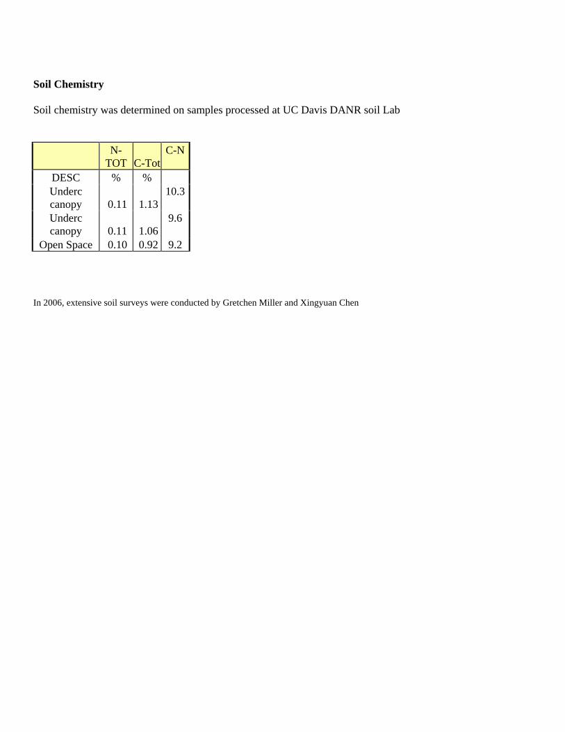
Soil Chemistry Soil chemistry was determined on samples processed at UC Davis DANR soil Lab

N-

TOT C-Tot C-N

DESC % % Underc canopy 0.11 1.13

10.3

Underc canopy 0.11 1.06

9.6

Open Space 0.10 0.92 9.2 In 2006, extensive soil surveys were conducted by Gretchen Miller and Xingyuan Chen

Soil Texture at Tonzi

0%

20%

40%

60%

80%

100%

1 11 21 32 42

Sample Number

Perc

enta

ge

ClaySiltSand

Porosity at Tonzi

0.00

0.10

0.20

0.30

0.40

0.50

0.60

0.70

1 11 21 31 41

Sample Number

Poro

sity

Climate There is no direct climate data from the ranches under investigation, but there is climate information in the region. There is a discontinued cooperative weather station in Ione, that gives us rain data between 1959 and 1977. There is no long term weather records at the site, but weather records from are available from the NCDC cooperative network for Ione, from 1959-1977 (t about 38.35°N 120.93°W. Height about 85m / 278 feet above sea level) Ione Average Rainfall

Jan Feb Mar Apr May Jun Jul Aug Sep Oct Nov Dec Year mm 99.6 83.9 76.8 51.9 10.7 3.1 0.3 5.2 5.5 31.6 94.5 94.6 558.7 inches 3.9 3.3 3.0 2.0 0.4 0.1 0.0 0.2 0.2 1.2 3.7 3.7 22.0 Source: derived from NCDC Cooperative Stations. 16 complete years between 1959 and 1977 a near by station, Ben Bolt, recorded There is a weather station at Pardee dam, which is south of the site, but on a similar altitudinal gradient, so the annual temperatures and rainfall sums are close. CAMP PARDEE, CALAVERAS COUNTY, CALIFORNIA USA Located at about 38.25°N 120.86°W. Height about 200m / 656 feet above sea level. Average Temperature

Jan Feb Mar Apr May Jun Jul Aug Sep Oct Nov Dec Year °C 7.3 10.0 11.6 14.5 18.5 22.6 25.8 25.1 22.6 18.3 12.1 7.8 16.3 °F 45.1 50.0 52.9 58.1 65.3 72.7 78.4 77.2 72.7 64.9 53.8 46.0 61.3 Source: derived from NCDC TD 9641 Clim 81 1961-1990 Normals. 30 years between 1961 and 1990 CAMP PARDEE, CALAVERAS COUNTY, CALIFORNIA USA Located at about 38.25°N 120.86°W. Height about 200m / 656 feet above sea level. Average Rainfall

Jan Feb Mar Apr May Jun Jul Aug Sep Oct Nov Dec Year mm 97.8 88.2 91.6 49.0 18.5 5.9 1.2 1.6 8.5 29.5 65.5 85.4 543.7 inches 3.9 3.5 3.6 1.9 0.7 0.2 0.0 0.1 0.3 1.2 2.6 3.4 21.4 Source8.0) DATA DESCRIPTION

Note the Pardee rainfall is 543 mm while the discontinued Ione site produced a mean of 558 mm per year. Hence we feel that the Pardee climate is representative of this site. In order to relate our data with other sites we include figures of Northern California rainfall.

Figure 24 source http://www.wrh.noaa.gov/Monterey/CA_NORTH.GIF

Using interpolation calculations of regional climate data using MtCLIME (Peter Thorton, NCAR; http://www.daymet.org/) we estimate that a 30 year mean of precipitation is about 611 mm. The mean maximum temperature is 22.2663, the mean minimum temperature is 8.0207 and the mean annual temperature is 18.3492

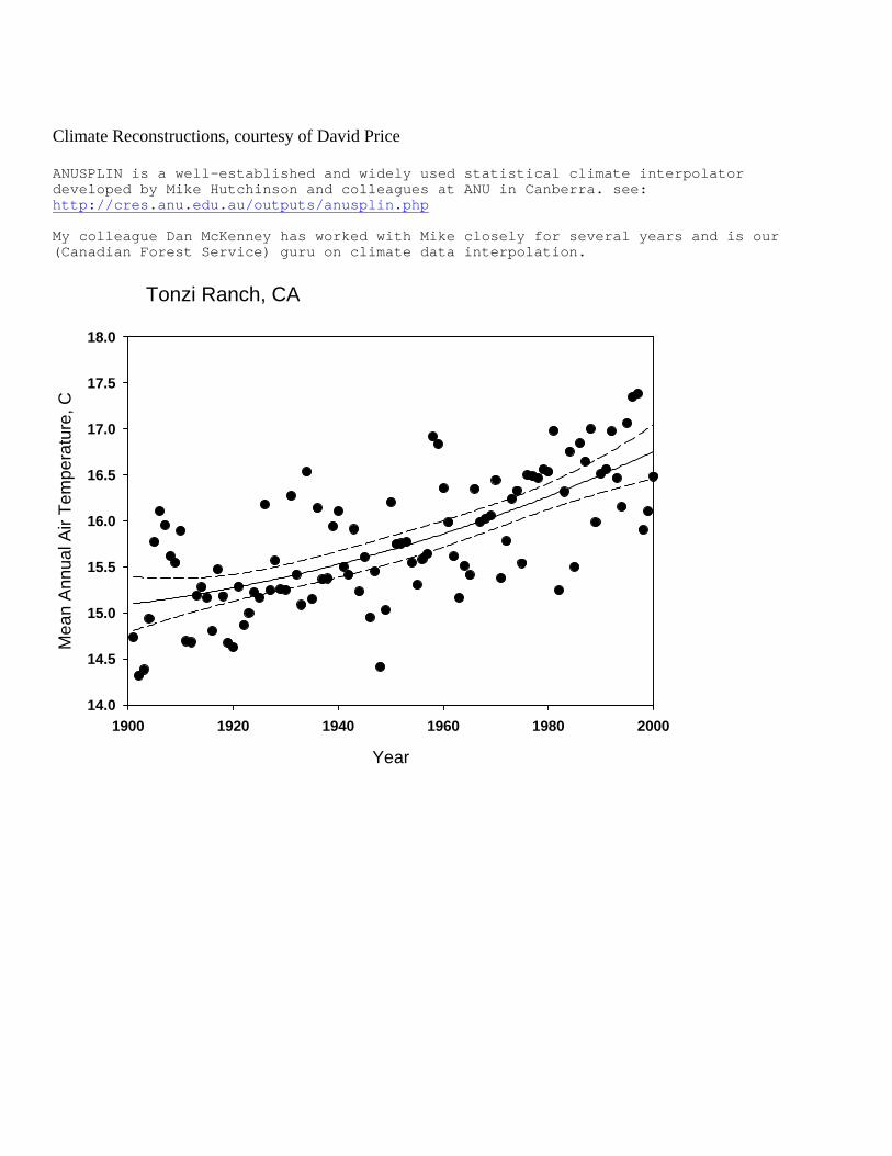
Climate Reconstructions, courtesy of David Price ANUSPLIN is a well-established and widely used statistical climate interpolator developed by Mike Hutchinson and colleagues at ANU in Canberra. see: http://cres.anu.edu.au/outputs/anusplin.php My colleague Dan McKenney has worked with Mike closely for several years and is our (Canadian Forest Service) guru on climate data interpolation.

Tonzi Ranch, CA

Year

1900 1920 1940 1960 1980 2000

Mea

n An

nual

Air

Tem

pera

ture

, C

14.0

14.5

15.0

15.5

16.0

16.5

17.0

17.5

18.0

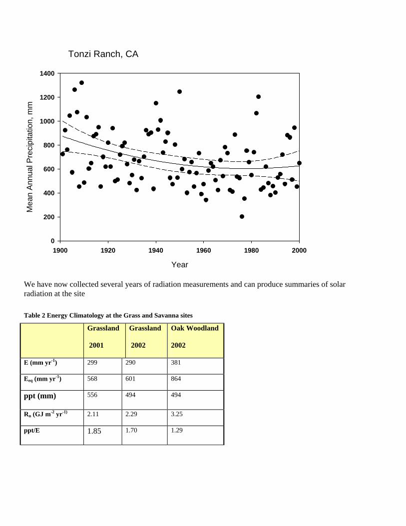
Tonzi Ranch, CA

Year

1900 1920 1940 1960 1980 2000

Mea

n A

nnua

l Pre

cipi

tatio

n, m

m

0

200

400

600

800

1000

1200

1400

We have now collected several years of radiation measurements and can produce summaries of solar radiation at the site Table 2 Energy Climatology at the Grass and Savanna sites

Grassland

2001

Grassland

2002

Oak Woodland

2002

E (mm yr-1) 299 290 381

Eeq (mm yr-1) 568 601 864

ppt (mm) 556 494 494

Rn (GJ m-2 yr-1) 2.11 2.29 3.25

ppt/E 1.85 1.70 1.29

Ppt/Eeq 0.98 0.82 0.57

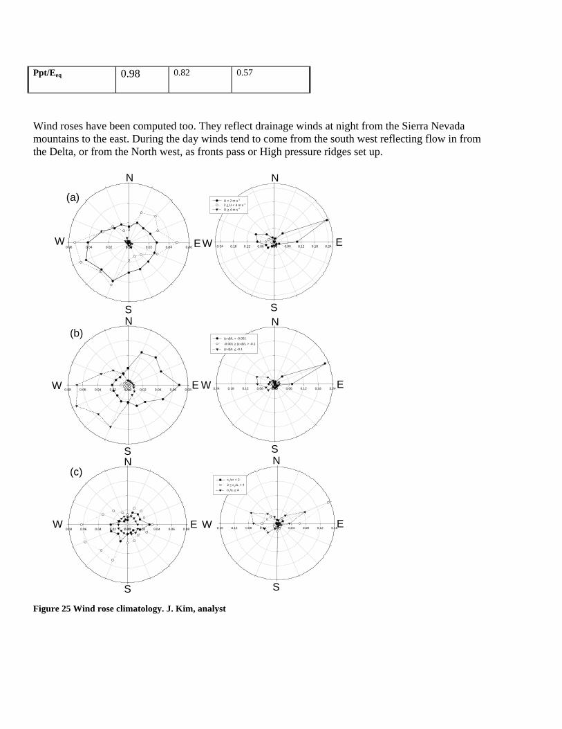
Wind roses have been computed too. They reflect drainage winds at night from the Sierra Nevada mountains to the east. During the day winds tend to come from the south west reflecting flow in from the Delta, or from the North west, as fronts pass or High pressure ridges set up.

0.00 0.02 0.04 0.06 0.080.000.020.040.060.08

0.00 0.02 0.04 0.06 0.080.000.020.040.060.08

0.00 0.06 0.12 0.18 0.240.000.060.120.180.24

U < 2 m s-1

2 < U < 4 m s-1

U > 4 m s-1

0.00 0.06 0.12 0.18 0.240.000.060.120.180.24

(z-d)/L > -0.001

-0.001 > (z-d)/L > -0.1

(z-d)/L < -0.1

0.00 0.04 0.08 0.12 0.160.000.040.080.120.16

σv/u∗ < 22 < σv/u* < 4σv/u* > 4

(a)

(b)

(c)

N

S

N

N

N

N

N

E

S

S

S S

S

E E

E

E

E

W

W

W

W

W

0.00 0.02 0.04 0.060.000.020.040.06

(a)

W

N

Figure 25 Wind rose climatology. J. Kim, analyst

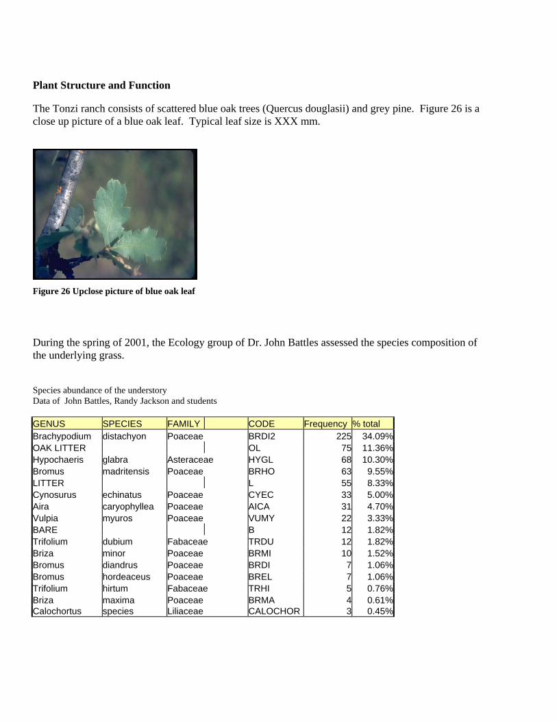
Plant Structure and Function The Tonzi ranch consists of scattered blue oak trees (Quercus douglasii) and grey pine. Figure 26 is a close up picture of a blue oak leaf. Typical leaf size is XXX mm.

Figure 26 Upclose picture of blue oak leaf

During the spring of 2001, the Ecology group of Dr. John Battles assessed the species composition of the underlying grass. Species abundance of the understory Data of John Battles, Randy Jackson and students GENUS SPECIES FAMILY CODE Frequency % total Brachypodium distachyon Poaceae BRDI2 225 34.09%OAK LITTER OL 75 11.36%Hypochaeris glabra Asteraceae HYGL 68 10.30%Bromus madritensis Poaceae BRHO 63 9.55%LITTER L 55 8.33%Cynosurus echinatus Poaceae CYEC 33 5.00%Aira caryophyllea Poaceae AICA 31 4.70%Vulpia myuros Poaceae VUMY 22 3.33%BARE B 12 1.82%Trifolium dubium Fabaceae TRDU 12 1.82%Briza minor Poaceae BRMI 10 1.52%Bromus diandrus Poaceae BRDI 7 1.06%Bromus hordeaceus Poaceae BREL 7 1.06%Trifolium hirtum Fabaceae TRHI 5 0.76%Briza maxima Poaceae BRMA 4 0.61%Calochortus species Liliaceae CALOCHOR 3 0.45%

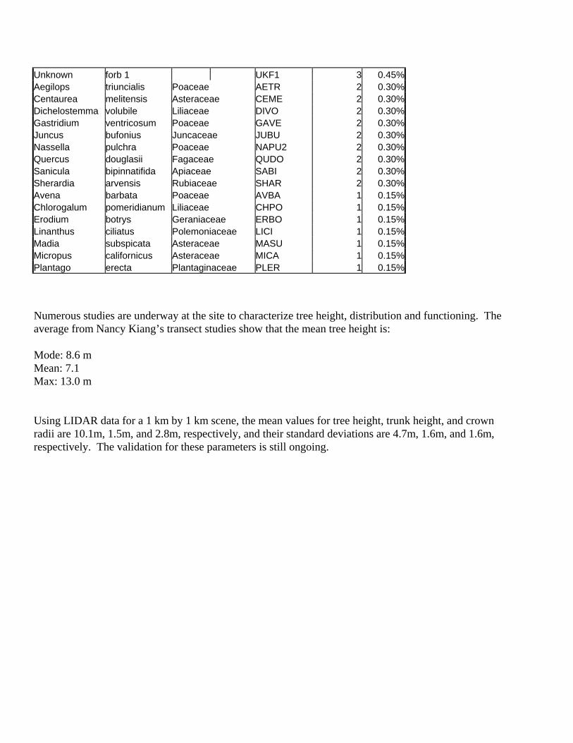
Unknown forb 1 UKF1 3 0.45%Aegilops triuncialis Poaceae AETR 2 0.30%Centaurea melitensis Asteraceae CEME 2 0.30%Dichelostemma volubile Liliaceae DIVO 2 0.30%Gastridium ventricosum Poaceae GAVE 2 0.30%Juncus bufonius Juncaceae JUBU 2 0.30%Nassella pulchra Poaceae NAPU2 2 0.30%Quercus douglasii Fagaceae QUDO 2 0.30%Sanicula bipinnatifida Apiaceae SABI 2 0.30%Sherardia arvensis Rubiaceae SHAR 2 0.30%Avena barbata Poaceae AVBA 1 0.15%Chlorogalum pomeridianum Liliaceae CHPO 1 0.15%Erodium botrys Geraniaceae ERBO 1 0.15%Linanthus ciliatus Polemoniaceae LICI 1 0.15%Madia subspicata Asteraceae MASU 1 0.15%Micropus californicus Asteraceae MICA 1 0.15%Plantago erecta Plantaginaceae PLER 1 0.15% Numerous studies are underway at the site to characterize tree height, distribution and functioning. The average from Nancy Kiang’s transect studies show that the mean tree height is: Mode: 8.6 m Mean: 7.1 Max: 13.0 m Using LIDAR data for a 1 km by 1 km scene, the mean values for tree height, trunk height, and crown radii are 10.1m, 1.5m, and 2.8m, respectively, and their standard deviations are 4.7m, 1.6m, and 1.6m, respectively. The validation for these parameters is still ongoing.

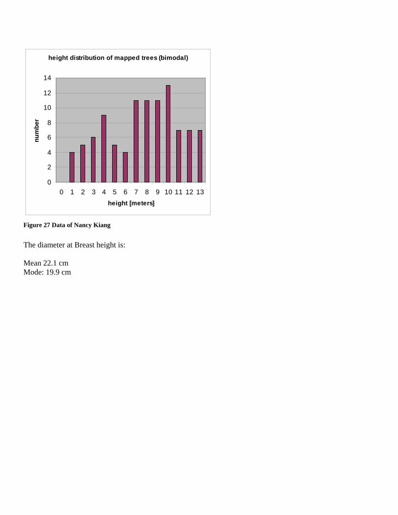
height distribution of mapped trees (bimodal)

0

2

4

6

8

10

12

14

0 1 2 3 4 5 6 7 8 9 10 11 12 13height [meters]

num

ber

Figure 27 Data of Nancy Kiang

The diameter at Breast height is: Mean 22.1 cm Mode: 19.9 cm

distribution of diameter at breast height (dbh)

0

0.02

0.04

0.06

0.08

0.1

0.12

0.14

0.16

0.18

0.2

0 5 10 15 20 25 30 35 40 45 50 55 60 65 70 75 80 85 90 95 100

dbh [cm]

frac

tion

mapped trees

all trees

Figure 28 Data of Nancy Kiang

Tonzi Ranch, blue oak savannadbh vs.tree height

y = 3.5266Ln(x) - 2.0738R2 = 0.7738

0

2

4

6

8

10

12

14

16

0 20 40 60 80 10

dbh [cm]

heig

ht [m

]

0

Figure 29 Data of Nancy Kiang

Figure 30 Qi Chen Analyst, LIDAR data

Figure 4. The relationship between crown radius and tree height.

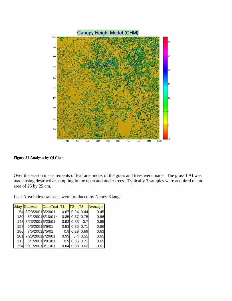
Figure 31 Analysis by Qi Chen

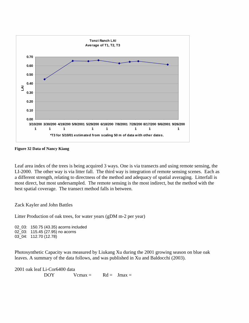
Over the season measurements of leaf area index of the grass and trees were made. The grass LAI was made using destructive sampling in the open and under trees. Typically 3 samples were acquired on an area of 25 by 25 cm. Leaf Area index transects were produced by Nancy Kiang Jday DateVal DateText T1 T2 T3 Average

54 3/23/2001 3/23/01 0.67 0.24 0.44 0.45130 5/1/2001 5/10/01* 0.85 0.37 0.75 0.66143 5/23/2001 5/23/01 0.93 0.33 0.7 0.65157 6/6/2001 6/6/01 0.93 0.35 0.71 0.66186 7/5/2001 7/5/01 0.9 0.29 0.69 0.63201 7/20/2001 7/20/01 0.99 0.4 0.55 0.65213 8/1/2001 8/01/01 0.9 0.35 0.71 0.65254 9/11/2001 9/11/01 0.84 0.38 0.62 0.61

Tonzi Ranch LAIAverage of T1, T2, T3

0.00

0.10

0.20

0.30

0.40

0.50

0.60

0.70

3/10/2001

3/30/2001

4/19/2001

5/9/2001 5/29/2001

6/18/2001

7/8/2001 7/28/2001

8/17/2001

9/6/2001 9/26/2001

*T3 for 5/10/01 estimated from scaling 50 m of data w ith other dates.

LAI

Figure 32 Data of Nancy Kiang

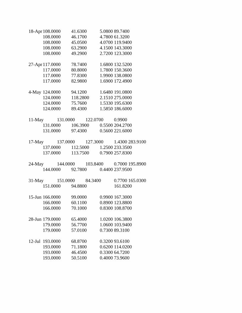
Leaf area index of the trees is being acquired 3 ways. One is via transects and using remote sensing, the LI-2000. The other way is via litter fall. The third way is integration of remote sensing scenes. Each as a different strength, relating to directness of the method and adequacy of spatial averaging. Litterfall is most direct, but most undersampled. The remote sensing is the most indirect, but the method with the best spatial coverage. The transect method falls in between. Zack Kayler and John Battles Litter Production of oak trees, for water years (gDM m-2 per year) 02_03: 150.75 (43.35) acorns included 02_03: 115.45 (27.95) no acorns 03_04: 112.70 (12.78) Photosynthetic Capacity was measured by Liukang Xu during the 2001 growing season on blue oak leaves. A summary of the data follows, and was published in Xu and Baldocchi (2003). 2001 oak leaf Li-Cor6400 data DOY Vcmax = Rd = Jmax =

18-Apr 108.0000 41.6300 5.0800 89.7400 108.0000 46.1700 4.7800 61.3200 108.0000 45.0500 4.0700 119.9400 108.0000 63.2900 4.1500 143.3000 108.0000 49.2900 2.7200 123.3000 27-Apr 117.0000 78.7400 1.6800 132.5200 117.0000 80.8000 1.7800 150.3600 117.0000 77.8300 1.9900 138.0800 117.0000 82.9800 1.6900 172.4900 4-May 124.0000 94.1200 1.6480 191.0800 124.0000 118.2800 2.1510 275.0000 124.0000 75.7600 1.5330 195.6300 124.0000 89.4300 1.5850 186.6000 11-May 131.0000 122.0700 0.9900 131.0000 106.3900 0.5500 204.2700 131.0000 97.4300 0.5600 221.6000 17-May 137.0000 127.3000 1.4300 283.9100 137.0000 112.5000 1.2500 233.3500 137.0000 113.7500 0.7900 257.8300 24-May 144.0000 103.8400 0.7000 195.8900 144.0000 92.7800 0.4400 237.9500 31-May 151.0000 84.3400 0.7700 165.0300 151.0000 94.8800 161.8200 15-Jun 166.0000 99.0000 0.9900 167.3000 166.0000 60.1100 0.8900 123.8800 166.0000 70.1000 0.8300 108.8700 28-Jun 179.0000 65.4000 1.0200 106.3800 179.0000 56.7700 1.0600 103.9400 179.0000 57.0100 0.7300 89.3100 12-Jul 193.0000 68.8700 0.3200 93.6100 193.0000 71.1800 0.6200 114.0200 193.0000 46.4500 0.3300 64.7200 193.0000 50.5100 0.4000 73.9600

23-Jul 204.0000 60.9000 0.3700 99.2300 204.0000 46.2700 0.3800 70.9900 204.0000 43.0200 0.3700 52.1200 30-Jul 211.0000 67.6800 0.5320 81.9700 211.0000 67.7700 0.2983 84.6400 9-Aug 221.0000 65.1700 0.5300 101.6200 221.0000 53.1200 0.7200 63.5800 16-Aug 228.0000 56.0000 0.2700 88.0000 228.0000 32.2400 0.4200 37.1700 228.0000 13.6300 0.6100 18.1400 23-Aug 235.0000 58.2800 0.6600 72.2000 235.0000 66.5800 0.4000 85.0000 30-Aug 242.0000 65.1300 0.6450 78.3900 242.0000 35.6400 0.7920 35.5500 242.0000 26.2100 0.4900 22.1500 242.0000 32.6100 0.3170 24.8300 6-Sep 249.0000 20.0900 0.4600 17.6600 249.0000 38.0900 0.2900 26.6700 249.0000 35.7600 0.3300 34.0300 13-Sep 256.0000 45.0500 0.4450 47.5300 256.0000 28.4500 0.6980 27.9100 256.0000 30.7100 0.5190 29.3000 - 8.1) Table Definition With Comments. '30 min data for AmeriFlux Web Page File names: These data are subject to several data filters. Filtout searches for outliers and replaces them with 9999. These periods are associated with rain events for the most part. Outliers are defined by limits set for variables according to variance, skewness and kurtosis thresholds. They differ for the sonic anemometer and infrared spectrometer. Filtturb is a filter that screens the data for limits according to Monin Obukov scaling theory. Mostly it looks for limits on the standard deviation of w. FiltCO2 screens the CO2 flux data for physiological limits. Data variables in tower0001dat files

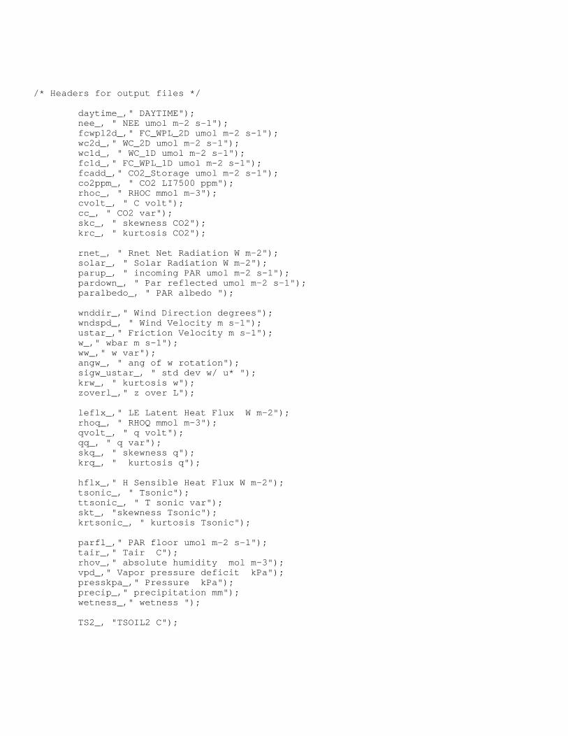
/* Headers for output files */ daytime_," DAYTIME"); nee_, " NEE umol m-2 s-1"); fcwpl2d_," FC_WPL_2D umol m-2 s-1"); wc2d_," WC_2D umol m-2 s-1"); wc1d_, " WC_1D umol m-2 s-1"); fc1d_," FC_WPL_1D umol m-2 s-1"); fcadd_," CO2_Storage umol m-2 s-1"); co2ppm_, " CO2 LI7500 ppm"); rhoc_, " RHOC mmol m-3"); cvolt_, " C volt"); cc_, " CO2 var"); skc_, " skewness CO2"); krc_, " kurtosis CO2"); rnet_, " Rnet Net Radiation W m-2"); solar_, " Solar Radiation W m-2"); parup_, " incoming PAR umol m-2 s-1"); pardown_, " Par reflected umol m-2 s-1"); paralbedo_, " PAR albedo "); wnddir_," Wind Direction degrees"); wndspd_, " Wind Velocity m s-1"); ustar_," Friction Velocity m s-1"); w_," wbar m s-1"); ww_," w var"); angw_, " ang of w rotation"); sigw_ustar_, " std dev w/ u* "); krw_, " kurtosis w"); zoverl_," z over L"); leflx_," LE Latent Heat Flux W m-2"); rhoq_, " RHOQ mmol m-3"); qvolt_, " q volt"); qq_, " q var"); skq_, " skewness q"); krq_, " kurtosis q"); hflx_," H Sensible Heat Flux W m-2"); tsonic_, " Tsonic"); ttsonic_, " T sonic var"); skt_, "skewness Tsonic"); krtsonic_, " kurtosis Tsonic"); parfl_," PAR floor umol m-2 s-1"); tair_," Tair C"); rhov_," absolute humidity mol m-3"); vpd_," Vapor pressure deficit kPa"); presskpa_," Pressure kPa"); precip_," precipitation mm"); wetness_," wetness "); TS2_, "TSOIL2 C");

TS4_, " TSOIL4 C"); TS8_, " TSOIL8 C"); TS16_," TSOIL16 C"); TS32_, " TSOIL32 C"); gsoil_, " G Soil Heat Flux: W m-2"); soilmoisturesfc_," soil moisture @ sfc %"); soilmoisture10_," soil moisture @ 10 cm %"); soilmoisture20_," soil moisture @ 20 cm %"); battery_volts," battery volts"); scan_," Number of scans"); 9.0) DATA MANIPULATIONS - 9.1) Formulas. Subroutine that computes covariances and applies gas law corrections static void process_flux() { float lambda, lfusion, rhoadry, rhomoist, tk, tksonic, cpair, rhovkg, spechum, sig; float wbarwpl, e_wpl_2d, e_wpl_1d, le1d, ewpl; float hflx1d, wtguess, wtguess_1d; float wqq, wqq1d, wtcorr1d, wtcorr2d; float term1, term2, terma, termb, sig16; float w_rhov_g_2d, w_rhov_g_1d, rhov_g; float rhoc_mg_m3; wtcorr2d=0; wtguess=0; wtcorr1d=0; wtguess_1d=0; tk=out.tair+273.15; tksonic=out.tsonic+273.15; if(fabs(out.tair)>50) { tk=tksonic; out.tair=out.tsonic; } /* latent heat of evaporation and fusion */ lambda = 3149000 - 2370 * tk; /* MJ kg-1 */ lfusion = 334000. ; if (tk < 273)

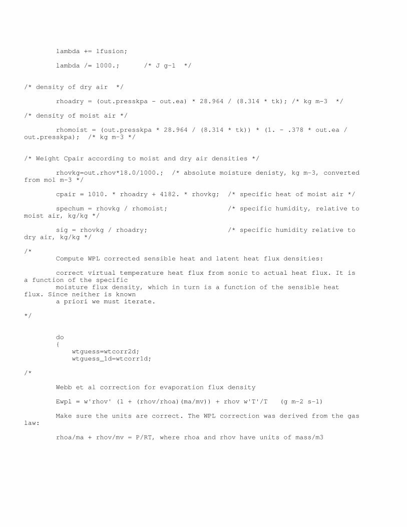
lambda += lfusion; lambda /= 1000.; /* J g-1 */ /* density of dry air */ rhoadry = (out.presskpa - out.ea) * 28.964 / (8.314 * tk); /* kg m-3 */ /* density of moist air */ rhomoist = (out.presskpa * 28.964 / (8.314 * tk)) * (1. - .378 * out.ea / out.presskpa); /* kg m-3 */ /* Weight Cpair according to moist and dry air densities */ rhovkg=out.rhov*18.0/1000.; /* absolute moisture denisty, kg m-3, converted from mol m-3 */ cpair = 1010. * rhoadry + 4182. * rhovkg; /* specific heat of moist air */ spechum = rhovkg / rhomoist; /* specific humidity, relative to moist air, kg/kg */ sig = rhovkg / rhoadry; /* specific humidity relative to dry air, kg/kg */ /* Compute WPL corrected sensible heat and latent heat flux densities: correct virtual temperature heat flux from sonic to actual heat flux. It is a function of the specific moisture flux density, which in turn is a function of the sensible heat flux. Since neither is known a priori we must iterate. */ do { wtguess=wtcorr2d; wtguess_1d=wtcorr1d; /* Webb et al correction for evaporation flux density Ewpl = w'rhov' (1 + (rhov/rhoa)(ma/mv)) + rhov w'T'/T (g m-2 s-1) Make sure the units are correct. The WPL correction was derived from the gas law: rhoa/ma + rhov/mv = P/RT, where rhoa and rhov have units of mass/m3

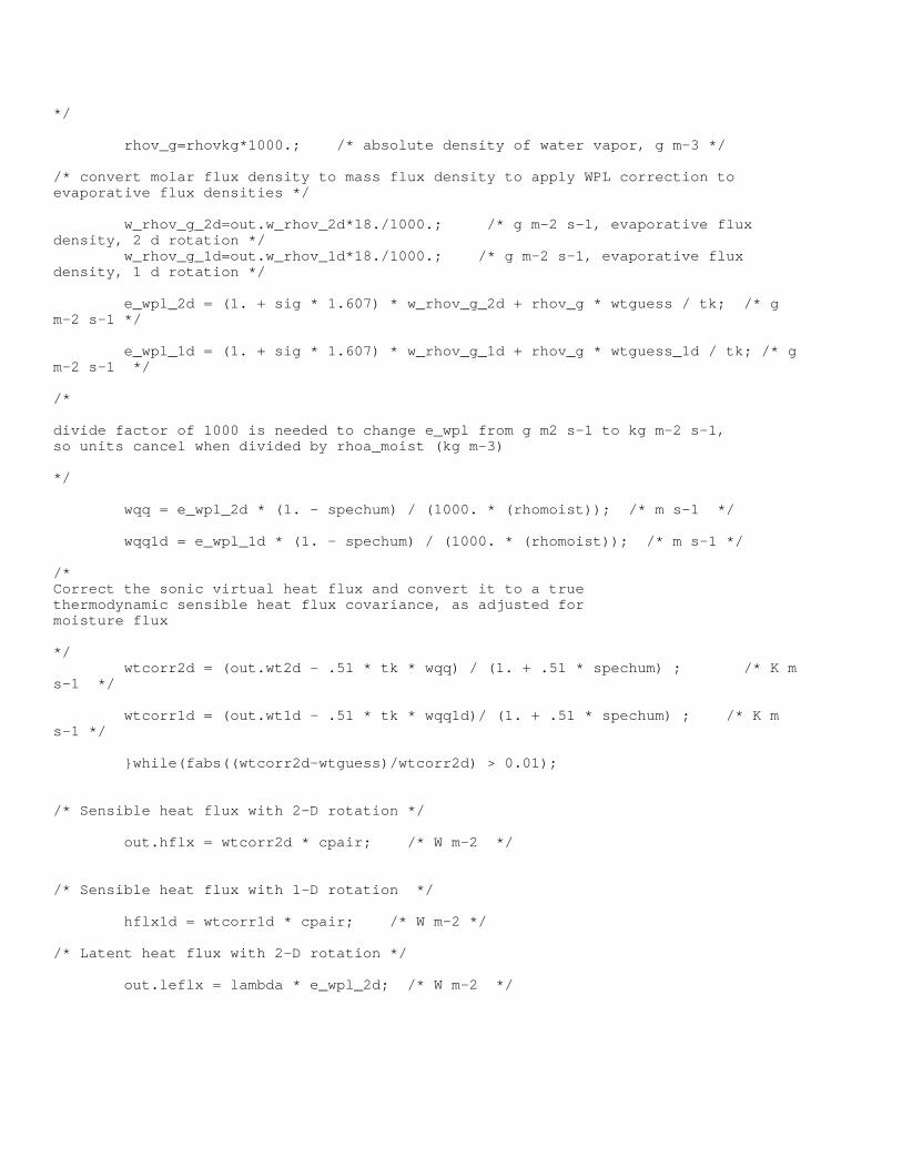
*/ rhov_g=rhovkg*1000.; /* absolute density of water vapor, g m-3 */ /* convert molar flux density to mass flux density to apply WPL correction to evaporative flux densities */ w_rhov_g_2d=out.w_rhov_2d*18./1000.; /* g m-2 s-1, evaporative flux density, 2 d rotation */ w_rhov_g_1d=out.w_rhov_1d*18./1000.; /* g m-2 s-1, evaporative flux density, 1 d rotation */ e_wpl_2d = (1. + sig * 1.607) * w_rhov_g_2d + rhov_g * wtguess / tk; /* g m-2 s-1 */ e_wpl_1d = (1. + sig * 1.607) * w_rhov_g_1d + rhov_g * wtguess_1d / tk; /* g m-2 s-1 */ /* divide factor of 1000 is needed to change e_wpl from g m2 s-1 to kg m-2 s-1, so units cancel when divided by rhoa_moist (kg m-3) */ wqq = e_wpl_2d * (1. - spechum) / (1000. * (rhomoist)); /* m s-1 */ wqq1d = e_wpl_1d * (1. - spechum) / (1000. * (rhomoist)); /* m s-1 */ /* Correct the sonic virtual heat flux and convert it to a true thermodynamic sensible heat flux covariance, as adjusted for moisture flux */ wtcorr2d = (out.wt2d - .51 * tk * wqq) / (1. + .51 * spechum) ; /* K m s-1 */ wtcorr1d = (out.wt1d - .51 * tk * wqq1d)/ (1. + .51 * spechum) ; /* K m s-1 */ }while(fabs((wtcorr2d-wtguess)/wtcorr2d) > 0.01); /* Sensible heat flux with 2-D rotation */ out.hflx = wtcorr2d * cpair; /* W m-2 */ /* Sensible heat flux with 1-D rotation */ hflx1d = wtcorr1d * cpair; /* W m-2 */ /* Latent heat flux with 2-D rotation */ out.leflx = lambda * e_wpl_2d; /* W m-2 */

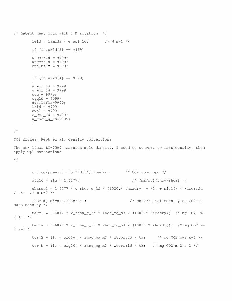
/* Latent heat flux with 1-D rotation */ le1d = lambda * e_wpl_1d; /* W m-2 */ if (in.wx2d[3] == 9999) { wtcorr2d = 9999; wtcorr1d = 9999; out.hflx = 9999; } if (in.wx2d[4] == 9999) { e_wpl_2d = 9999; e_wpl_1d = 9999; wqq = 9999; wqq1d = 9999; out.leflx=9999; le1d = 9999; ewpl = 9999; e_wpl_1d = 9999; w_rhov_g_2d=9999; } /* CO2 fluxes, Webb et al. density corrections The new Licor LI-7500 measures mole density. I need to convert to mass density, then apply wpl corrections */ out.co2ppm=out.rhoc*28.96/rhoadry; /* CO2 conc ppm */ sig16 = sig * 1.6077; /* (ma/mv)(rhov/rhoa) */ wbarwpl = 1.6077 * w_rhov_g_2d / (1000.* rhoadry) + (1. + sig16) * wtcorr2d / tk; /* m s-1 */ rhoc_mg_m3=out.rhoc*44.; /* convert mol density of CO2 to mass density */ term1 = 1.6077 * w_rhov_g_2d * rhoc_mg_m3 / (1000.* rhoadry); /* mg CO2 m-2 s-1 */ terma = 1.6077 * w_rhov_g_1d * rhoc_mg_m3 / (1000. * rhoadry); /* mg CO2 m-2 s-1 */ term2 = (1. + sig16) * rhoc_mg_m3 * wtcorr2d / tk; /* mg CO2 m-2 s-1 */ termb = (1. + sig16) * rhoc_mg_m3 * wtcorr1d / tk; /* mg CO2 m-2 s-1 */

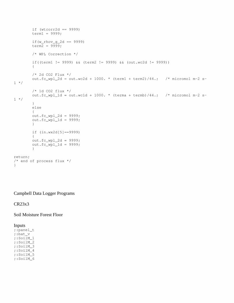
if (wtcorr2d == 9999) term1 = 9999; if(w_rhov_g_2d == 9999) term2 = 9999; /* WPL Correction */ if((term1 != 9999) && (term2 != 9999) && (out.wc2d != 9999)) { /* 2d CO2 Flux */ out.fc_wpl_2d = out.wc2d + 1000. * (term1 + term2)/44.; /* micromol m-2 s-1 */ /* 1d CO2 flux */ out.fc_wpl_1d = out.wc1d + 1000. * (terma + termb)/44.; /* micromol m-2 s-1 */ } else { out.fc_wpl_2d = 9999; out.fc_wpl_1d = 9999; } if (in.wx2d[5]==9999) { out.fc_wpl_2d = 9999; out.fc_wpl_1d = 9999; } return; /* end of process flux */ } Campbell Data Logger Programs CR23x3 Soil Moisture Forest Floor Inputs ;:panel_t ;:bat_v ;:SoilM_1 ;:SoilM_2 ;:SoilM_3 ;:SoilM_4 ;:SoilM_5 ;:SoilM_6

;:SoilM_7 ;:q_line ;:NR_1 ;:NR_2 ;122 Output_Table 30.00 Min ;1 122 L ;2 Day_RTM L ;3 Hour_Minute_RTM L ;4 panel_t_AVG L ;5 bat_v_AVG L ;6 SoilM_1_AVG L ;7 SoilM_2_AVG L ;8 SoilM_3_AVG L ;9 SoilM_4_AVG L ;10 SoilM_5_AVG L ;11 SoilM_6_AVG L ;12 SoilM_7_AVG L ;13 q_line_AVG L ;14 NR_1_AVG L ;15 NR_2_AVG L Met on Tower CR23X6 Input Table ;:Panel_T ;:Batt_Volt ;:Pricip_mm ;:Par_up ;:Par_Dn ;:Par_Calib ;:Pyranom ;:Net_Rad ;:Temp_Amb ;:RH ;:L_PAR1 ;:L_PAR2 ;131 Output_Table 30.00 Min ;1 131 L ;2 Day_RTM L ;3 Hour_Minute_RTM L ;4 Panel_T_AVG L ;5 Batt_Volt_AVG L ;6 Pricip_mm_TOT L ;7 Par_up_AVG L ;8 Par_Dn_AVG L ;9 Par_Calib_AVG L ;10 Pyranom_AVG L ;11 Net_Rad_AVG L ;12 Temp_Amb_AVG L ;13 RH_AVG L ;14 Par_up_STD L

;15 Par_Dn_STD L ;16 Par_Calib_STD L ;17 Pyranom_STD L ;18 Net_Rad_STD L ;19 Temp_Amb_STD L ;20 RH_STD L ; The new wind speed profile system has been installed on 5 levels. The data logger program was written for 6 levels. The lowest level is labeled 1 and the highest is labeled 6. Output is as follows: Final Storage Label File for: WSP1.CSI Date: 8/1/2003 Time: 12:09:19 105 Output_Table 30.00 Min 1 105 L 2 Day_RTM H 3 Hour_Minute_RTM H 4 Panel_T_AVG H 5 Batt_V_AVG H 6 WS_1_AVG H 7 WS_2_AVG H 8 WS_3_AVG H 9 WS_4_AVG H 10 WS_5_AVG H 11 WS_6_AVG H 12 WD_1_AVG H 13 WD_2_AVG H 14 WD_3_AVG H 15 WD_4_AVG H 16 WD_5_AVG H 17 WD_6_AVG H 18 WS_1_STD H 19 WS_2_STD H 20 WS_3_STD H 21 WS_4_STD H 22 WS_5_STD H 23 WS_6_STD H 24 WD_1_STD H 25 WD_2_STD H 26 WD_3_STD H 27 WD_4_STD H 28 WD_5_STD H 29 WD_6_STD H 30 WS_1_MAX H

31 WS_1_Hr_Min_MAX H 32 WS_2_MAX H 33 WS_2_Hr_Min_MAX H 34 WS_3_MAX H 35 WS_3_Hr_Min_MAX H 36 WS_4_MAX H 37 WS_4_Hr_Min_MAX H 38 WS_5_MAX H 39 WS_5_Hr_Min_MAX H 40 WS_6_MAX H 41 WS_6_Hr_Min_MAX H 42 WD_1_MAX H 43 WD_1_Hr_Min_MAX H 44 WD_2_MAX H 45 WD_2_Hr_Min_MAX H 46 WD_3_MAX H 47 WD_3_Hr_Min_MAX H 48 WD_4_MAX H 49 WD_4_Hr_Min_MAX H 50 WD_5_MAX H 51 WD_5_Hr_Min_MAX H 52 WD_6_MAX H 53 WD_6_Hr_Min_MAX H 54 WS_1_MIN H 55 WS_1_Hr_Min_MIN H 56 WS_2_MIN H 57 WS_2_Hr_Min_MIN H 58 WS_3_MIN H 59 WS_3_Hr_Min_MIN H 60 WS_4_MIN H 61 WS_4_Hr_Min_MIN H 62 WS_5_MIN H 63 WS_5_Hr_Min_MIN H 64 WS_6_MIN H 65 WS_6_Hr_Min_MIN H 66 WD_1_MIN H 67 WD_1_Hr_Min_MIN H 68 WD_2_MIN H 69 WD_2_Hr_Min_MIN H 70 WD_3_MIN H 71 WD_3_Hr_Min_MIN H 72 WD_4_MIN H 73 WD_4_Hr_Min_MIN H 74 WD_5_MIN H 75 WD_5_Hr_Min_MIN H 76 WD_6_MIN H 77 WD_6_Hr_Min_MIN H - 9.1.1 Derivation Techniques/Algorithms. none provided. - 9.2) Data Processing Sequence.

Flux covariances are computed in the field by the data acquisition program. Back at home, calibrations are double and triple checked by comparing old and new calibrations and by comparing the mean response of the scalar flux sensors against independent meteorological instruments. Tests are made for energy balance closure to ensure that the data are of reliable quality. Programs are then run to delete periods when the sensors were off line, off range, being maintained or un-reliable due to rain or instrument malfunction.

- 9.2.1 Processing Steps and Data Sets.

Flux data: all the flux data are organized in the following way Typically, each folder has subfolder Floor_2001 eg. Floor_2001 Floor_2002 Datalogger Notes Floor_2003 Floor_C++ code Floor_2004 flux Floor_interannual flux_fromfield met Tower_2001 raw Tower_2002 sapflow Tower_2003 Sum_data Tower_2004 Tower_interannual Vaira_2003 Datalogger Notes flux Vaira_2000 flux_fromfield Vaira_2001 met Vaira_2002 raw Vaira_2003 Sum_data Vaira_2004 Vaira03_C code Vaira_interannual

In the subfolder, Datalogger Notes, you will find two files called, cr10x_heading 2001_fl.xls cr23x_heading 2001_fl.xls They are very important files, containing all the information of outputs from soil and met sensors for each EC system. They also contain the information about when Ted adds new sensors or removes sensors, or rearranges the sequence of output, or changes the output from engineering unit to mv. Sometime I also include the calibration factor, but if not, it should be in the subroutine (calibration) of C++ program file. In the subfolder, Floor_C++ code, It contains two C++ code files, raw_floor2001.c for raw data processing and flux_floor2001.c for flux computation Subfolder, flux, contains all the output files from the raw_floor2001.c code, including;

*.spk *.err_dspk *.flx_dspk *.nrt_dspk Subfolder, flux_fromfield, contains all the *.NRT, *.FLX, *.ERR files, they are from field laptop. They are just for diagnostic purpose, you don’t need them to compute the EC flux. Subfolder, met, contain all the daily met and soil data. For examples, tz2_01DOY.10x and tz3_01DOY.23x Subfolder, raw, contains no file. This folder I used to prepare, rename and clean raw files. After done, I copy all the raw data files to F: drive. Subfolder, Sum_data, contains all the sigmaplot files and the output file from flux_floor2001.c C++ code; i.e. Tonzi_understory2001.dat. In folders, Tower_2003 and Tower_2004, I have two additional subfolders, called CO2Profile and Windprofile, which contain all the CO2 and wind profiles data. In folders, Floor_interannual, Tower_interannual, Vaira_interannual, I have some files for the interannual comparison of flux (Fc, LE, H, and radiation components) for each EC system. All the EC raw data, processed data, met and soil data have been backuped on H205-3 computer. In the folder, LI_COR7500, it contains all the calibration data for our six licor 7500. Section two: Process EC flux Data preparation a. Met and soil data: Break down to daily files if the laptop is not working around mid-night. Also make sure

each met and soil file start with 0030 and end with 2400. b. Raw data file: currently, the names for all the raw data file generated by gillsonic.exe from three EC

systems are as following; DOY Vaira Tower Floor 1-9 V?time.raw T?time.raw F?time.raw 10-99 V??time.raw T??time.raw F??time.raw 100-365 V???time.raw T???time.raw F???time.raw * ? represents DOY time: 4 digits time

C++ code can’t process the raw data with this kind file names. To have the right file name as I listed in the following table, I create a batch file to rename all the files. How to create the batch file? Please read the email message at your left on the glass door of the cabinet. It is very simple and fast!

After rename DOY Vaira Tower Floor 1-9 V00?time.raw T00?time.raw F00?time.raw

10-99 V0??time.raw T0??time.raw F0??time.raw 100-365 V???time.raw T???time.raw F???time.raw

Also another minor thing you need to do is to rename all the raw data file VDOY0000.raw by add 1 on DOY. I think these file naming problems can be fixed by modifying the source code of gillsonic.exe. If more than one raw data file in 0.5 hr, I delete one. This could happen at 4:30am when watchdog program reboots the EC systems, or when we are out there to download the data. I do all these raw data preparation on folders on C: Drive, then copy to appropriated folder on F: Drive. Last thing is to run raw_floor2004.exe and flux_floor2004.exe C++ code to compute the flux. Plot the flux using sigma-plot, check all the flux data (Fc, LE, H, and G), CO2 and water vapor concentrations, met and soil data, make sure they are all in the right ranges. If any data you think it is not right, talk to Dennis or Ted. 10.0) ERRORS - 10.1) Sources of Error. - 10.2) Quality Assessment. Surface energy balance is tested by comparing measurements of available energy against the sum of latent and sensible heat flux.

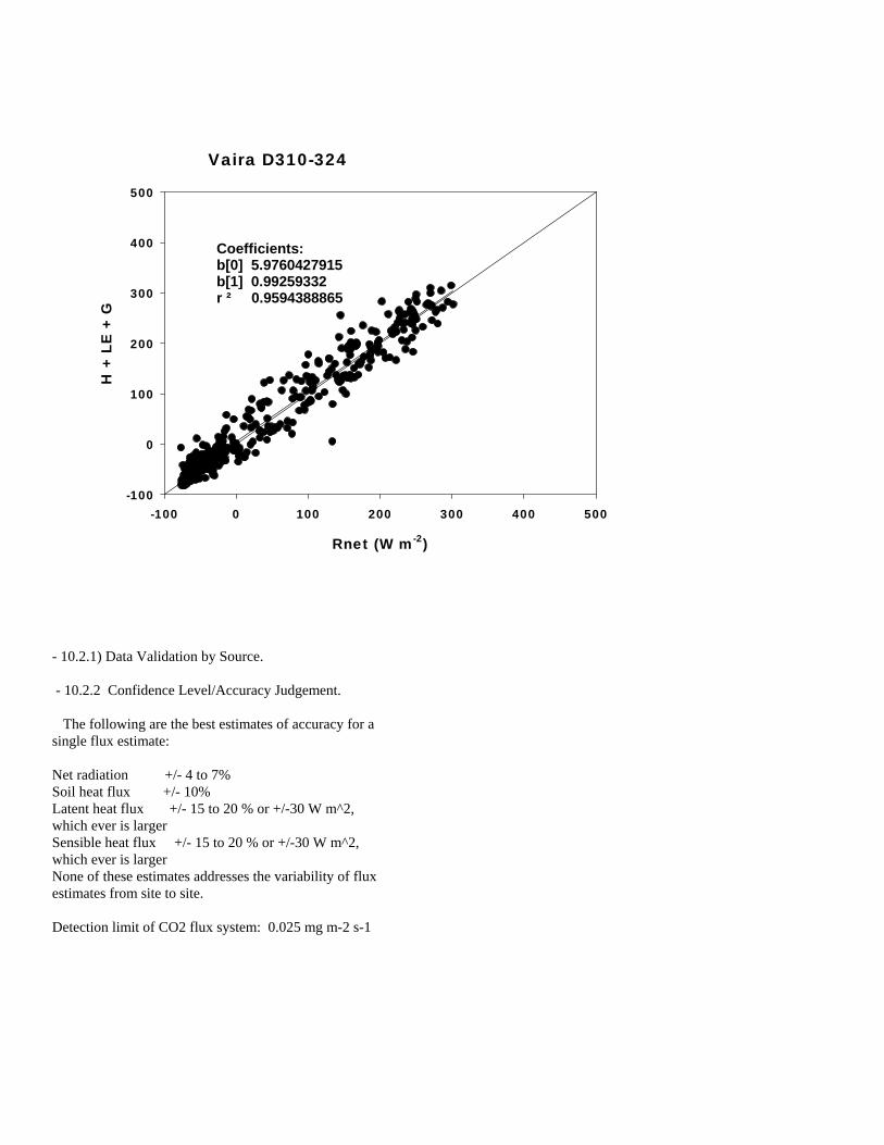
Vaira D310-324

Rnet (W m-2)

-100 0 100 200 300 400 500

H +

LE

+ G

-100

0

100

200

300

400

500

Coefficients:b[0] 5.9760427915b[1] 0.99259332r ² 0.9594388865

- 10.2.1) Data Validation by Source. - 10.2.2 Confidence Level/Accuracy Judgement. The following are the best estimates of accuracy for a single flux estimate: Net radiation +/- 4 to 7% Soil heat flux +/- 10% Latent heat flux +/- 15 to 20 % or +/-30 W m^2, which ever is larger Sensible heat flux +/- 15 to 20 % or +/-30 W m^2, which ever is larger None of these estimates addresses the variability of flux estimates from site to site. Detection limit of CO2 flux system: 0.025 mg m-2 s-1

The intermittency of turbulence limits the sampling error of turbulent fluxes to 10 to 20%. On top of this we have to deal with measurement errors. Fortunately, lots of statistically averaging reveals stable fluxes and small bias errors (< 12%) on the surface energy fluxes. - 10.2.3 Measurement Error for Parameters and Variables. 11.0) NOTES 11.1) Known Problems With The Data. As the duration of the experiment has continued we are finding that soil heat flux is biased low at the Vaira and Tonzi ranches. The soil heat flux plates are in cow proof enclosures, so insulating biomass is accumulating over the sensors and is insulating them. Plus grass is taller in the cow proof areas, so less energy reaches the ground. We have seen energy balance closure degrade from near 95% at the beginning of the Vaira study to about 75% circa 2003. The radiation boom from the tower was initially only a meter away. Plus the tower was put in the open, so the values of albedo and net radiation may be biased. In the spring of 2004 we extended the radiation boom out about 3 m to give the sensors a better view of the soil system. 11.2) Usage Guidance. 12.0) REFERENCES Publications Generated From this Project Baldocchi, D.D., Xu, L. and Kiang, N., 2004. How plant functional-type, weather, seasonal drought, and

soil physical properties alter water and energy fluxes of an oak-grass savanna and an annual grassland. Agricultural and Forest Meteorology, 123(1-2): 13-39.

Tang J, Baldocchi D D., Qi Y, Xu L. 2003. Assessing soil CO2 efflux using continuous measurements of

CO2 within the soil profile with small solid-state sensors. Agricultural and Forest Meteorology (submitted, Dec. 2002; Accepted March, 2003).

Xu L, Baldocchi DD. 2003. Seasonal trend of photosynthetic parameters and stomatal conductance of

blue oak (Quercus douglasii) under prolonged summer drought and high temperature Tree Physiology 23, 865-877.

Xu, L. and Baldocchi, D.D., 2004. Seasonal variation in carbon dioxide exchange over a Mediterranean

annual grassland in California. Agricultural and Forest Meteorology, 123(1-2): 79-96.

Baldocchi, D.D., Tang, J. and Xu, L., 2006. How Switches and Lags in Biophysical Regulators Affect Spatio-Temporal Variation of Soil Respiration in an Oak-Grass Savanna. Journal Geophysical Research, Biogeosciences, 111: G02008, doi:10.1029/2005JG000063.

Baldocchi, D. and Xu, L., 2005. Carbon excahnge of deciduous broadleaved forests in temperature and

Mediterranean regions. In: H. Griffiths and P. Jarvis (Editors), The Carbon Balance of forest biomes. Taylor and Francis, Andover, Hampshire, United Kingdom, pp. 187-216.

Baldocchi, D.D. et al., 2005. Predicting the onset of net carbon uptake by deciduous forests with soil

temperature and climate data: a synthesis of FLUXNET data. International Journal of Biometeorology, 49(DOI: 10.1007/s00484-005-0256-4): 377-387.

Acknowledgements Ranch Owner: Mr Russell Tonzi Ione Ca Field Assistance: Liukang Xu, Ted Hehn, Nancy Kiang, Lianhong Gu, Jianwu Tang, Kevin Tu, Francesca Ponti, Laurent Misson, John Battles, Randy Jackson. Funding US Dept of Energy, Terrestrial Carbon Program, Roger Dahlman administrator California Agricultural Experiment Station Kearney Soil Science Foundation, Kate Scow WESTGEC, NIGEC, Susan Ustin adminsitrator Contribution to AmeriFlux and Fluxnet programs