Documentation and User Manual - Southwest … Kinematic Runoff and Erosion Model: Documentation and...

$% United States)J) Department of91 Agriculture

AgriculturalResearchService

ARS-77

March 1990

KINEROS,A Kinematic Runoffand Erosion Model

Documentation and User Manual

ABSTRACT

Woolhiser, D.A., R.E. Smith, and D.C. Goodrich. 1990. KINEROS,A Kinematic Runoff and Erosion Model: Documentation and User

Manual. U.S. Department of Agriculture, Agricultural ResearchService, ARS-77, 130 pp.

The kinematic runoff and erosion model KINEROS is an event-

oriented, physically based model describing the processes ofinterception, infiltration, surface runoff, and erosion fromsmall agricultural and urban watersheds. The watershed isrepresented by a cascade of planes and channels; and the partialdifferential equations describing overland flow, channel flowand erosion, and sediment transport are solved by finitedifference techniques. Spatial variability of rainfall andinfiltration, runoff, and erosion parameters can beaccommodated. KINEROS may be used to determine the effects ofvarious artificial features such as urban developments, smalldetention reservoirs, or lined channels on flood hydrographs andsediment yield.

KEYWORDS: Erosion, infiltration, pond, reservoir,sedimentation, simulation, surface runoff

Computer printouts are reproduced essentially as supplied by theauthors.

No warranties, expressed or implied, are made that the computerprograms described in this publication are free from errors orare consistent with any particular standard of programminglanguage, or that they will meet a user's requirement for anyparticular application. The U.S. Department of Agriculturedisclaims all liability for direct or consequential damagesresulting from the use of the techniques or programs documentedherein.

Trade names are used in this publication solely to providespecific information. Mention of a trade name does notconstitute a guarantee or warranty of the product by the U.S.Department of Agriculture or an endorsement by the Departmentover other products not mentioned.

Copies of this publication may be purchased from the NationalTechnical Information Service, 5285 Port Royal Road,Springfield, VA 22161.

ARS has no additional copies for free distribution.

United StatesDepartment ofAgriculture

AgriculturalResearchService

ARS-77

KINEROS,A Kinematic Runoff

and Erosion Model

Documentation and User Manual

ii

PREFACE

This manual is designed to provide a brief description of thecomponents of the kinematic runoff and erosion model KINEROS.It also describes the program structure and the data setrequired to represent a catchment and provides guidance forestimating model parameters. The FORTRAN program for KINEROS isincluded in the files KINHYDl.FOR, KINSEDl.FOR, and KINTEMl.FORon the enclosed diskette. Input and output files for theexamples are also on the diskette. Instructions and anyrevisions are included in the file README.DOC.

CONTENTS

Introduction 1

Theory 3Introduction 3

Interception 4Infiltration 6

Hortonian overland flow 15

Channel routing 20Reservoir routing 25Erosion and sediment transport 26

KINEROS program documentation 34Program description 34Creation of input files 39Infiltration parameter estimation 49Erosion parameters 50Describing the geometry and character

istics of a pond 58Program output 59

Examples using hypothetical watersheds 63Example 1 63Example 2 68Example 3 83

Examples using real watersheds 91Example 4 91Example 5 109

Concluding remarks 121

Literature cited 122

Appendix: Sediment transport capacityrelations available in KINEROS 128

iii

iv

SYMBOLS

A = Cross sectional area of water in a channel [L2]

a «=• Fitting parameter in infiltration recovery equation

B - G(0 - 6.) [L]s 1 l J

b = Trapezoidal channel dimension [L]

BW = Channel bottom width [L]

1/2 -1C = Chezy friction coefficient [L ' T ]

C. = Weir coefficient

c9 = Weir equation exponent

C = Drag coefficient

c- =- Coefficient in splash erosion equation

c = Hydraulic erosion transfer rate coefficient [T ]

c, = Damping coefficient for splash erosion

C = Equilibrium sediment concentrationmx ^

c = Parameter in Bagnold/Kilinc sediment transport equation

C = Sediment concentrations

c = Parameter in tractive force equation

D = Diameter of circular conduit [L]

d = Particle diameter [L]

d = Raindrop diameter [L]

D50 =* Median particle diameter

2 -1e =» Rate of erosion of soil bed [L T ]

F = Amount of rain infiltrated [L]

f' - Infiltration rate [LT~ ]

f = Denotes functional relationship

-1f - Infiltration capacity [LT ]

f , = Fractional clay contentcl J

t = Darcy-Weisbach friction factor

F = Ponding depth [L]

G = Effective net capillary drive [L]

_2g = Acceleration of gravity [LT ]

2 -1g, = Hydraulic erosion rate [L T ]

2 -1g =» Splash erosion rate [L T ]

h = Depth of surface runoff [L]

h = Hydraulic depth of circular conduit [L]

h = Elevation of reservoir water surface [L]

h = Reservoir outflow structure notch elevation [L]z L J

I = Interception depth [L]

k = Dimensionless parameter in laminar flow equation

k(h) = Function describing reduction in splash erosion aswater depth, h, increases

k = Dimensionless parameter without raindrop impact effect

-1K = Effective saturated hydraulic conductivity [LT ]

vi

K .. = Soil erodibility factor in USLEusle J

K(V>) = Hydraulic conductivity function [LT ]

L = Length of plane or channel [L]

m = Exponent in relationship between runoff rate andstorage per unit area

n = Manning's n

p = Channel wetted perimeter [L]

p = Effective channel wetted perimeter for infiltration [L]

P = Volume of rock in unit volume of soil

2 -1Q - Surface runoff discharge per unit width [L T ] or

3 -1channel discharge [L T ]

q = Lateral inflow rate to a plane (Rainfall rate minus

infiltration rate.) [LT ]

2 -1q = Lateral inflow rate to channel [L T 1^c

3 -1q = Flow rate into a reservoir [L T ]

q = Sediment transport capacity per unit width-overland

flow [L2T_1]

3 -1q = Flow rate out of a reservoir [L T ]

2 -1q = Rate of lateral sediment inflow [L T 1^s

R = Hydraulic radius [L]

r = Rainfall rate [LT~ ]

R = Reynolds number

R = Particle Reynolds numbern J

r «= Weight of rock per unit weight of soil

S = Slope of plane or channel

S = Relative saturation at field capacity

S_ = Friction slope

S = Initial relative saturation

S Maximum relative saturationmax

S = Residual relative saturation

S = Particle specific gravity

t = Time [T]

t = Time to equilibrium for a plane [T^

t = Ponding time [T]

u = Local vertically averaged velocity [LT~

u^ = Shear velocity [LT- ]

3V = Reservoir volume [L ]

V = Relative volume of rock in soil

vg = Particle fall velocity [LT-1]

W = Width of plane [L]

x = Distance [L]

ZL = Side slope of left side of a trapezoidal channel

ZR = Side slope of right side of a trapezoidal channel

a =* Coefficient in relationship between runoff rate andstorage per unit area

vii

viii

p = Exponent in sediment transport relationship

7 = Exponent in sediment transport relationship

7 = Specific weight of water

8 - Exponent in sediment transport relationship

At = Finite difference time increment [T]

Ax = Finite difference length increment [L]

e = Exponent in sediment transport relationship

rj = Infiltration recovery rate factor

8 =• Relative volumetric soil water content, dimensionless

8 = Intersection angle in conduits

8. = Initial soil water content, dimensionless

8 = Maximum soil water content under imbibition

8 = Weighting factor 0 < 8 < 1w ° ° w

2r = Critical shear stress [L /Tlc

2r = Bed shear stress [L /T]

o

2 -1v = Kinematic viscosity [L T ]

-3p = Sediment particle density [ML ]

4> = Porosity

<i_ =» Factor to reduce K ., for mulch, etc.*r usle

<f> = Factor to reduce hydraulic erosion for mulch, etc

tf> = Soil matric potential [L]

w = Coefficient in sediment transport relationship

KINEROS, A KINEMATIC RUNOFF AND EROSION MODEL: DOCUMENTATIONAND USER MANUAL

D.A. Woolhiser, R.E. Smith, and D.C. Goodrich

INTRODUCTION

Engineers and soil conservationists often need to estimaterunoff rates and volumes from ungaged watersheds. Traditionalformula methods are useful for some purposes, but for manyobjectives more precise knowledge is required about thehydrologic response of a watershed or model sensitivity tovarious physical factors or assumptions. For this purpose,physically based distributed models of runoff are becoming morewidely used. This report describes such a model, calledKINEROS.

Since about 1970, the kinematic wave approximation has become awidely used method to simulate the movement of rainfall excesswater over the land surface and through small channels.Although this method requires simplifying assumptions comparedto more complete theory, its hydraulic requirements are wellestablished (Wooding 1965, Woolhiser and Liggett 1967). It hasbeen extensively verified by experiment (Woolhiser et al. 1970,Morgali 1970, Schreiber 1970, Kibler and Woolhiser 1970, Roveyand Woolhiser 1977). This method was applied to an arbitrarynetwork of planes and channels in a computer model called KINGENby Rovey et al. (1977). This model employed a computer solutionderived model for infiltration to simulate the production ofrunoff, and it was intended for rural or urban runoff studiesusing a design storm.

Since publication of that document (Rovey et al. 1977), themodel has been modified--the most notable modifications beingthe inclusion of simulation of erosion and sediment transport,revision of the infiltration component, and inclusion of a pondelement. The model, now called KINEROS, has attained somepopularity and has been used by research and consulting groups.KINEROS simulates the response of a catchment, whose

Woolhiser and Goodrich are hydraulic engineerswith USDA-ARS, Aridland Watershed ManagementResearch, 2000 East Allen Road, Tucson, AZ85719; Smith is a hydraulic engineer with USDA-ARS, Hydro-Ecosystems Research Unit, P.O. BoxE, Ft. Collins, CO 80522.

We gratefully acknowledge the assistance ofVirginia Ferreira, USDA-ARS, Fort Collins, CO,and Timothy Keefer, USDA-ARS, Tucson, AZ incomputer programming, to Laura Yohnka, USDA-ARS, Tucson, AZ for assistance in preparingthe manuscript for publication, and toAlice Kunishi and Elizabeth Sanford, USDA-ARS,Beltsville, MD, for outstanding editing.

configuration is defined by the user, to the occurrence of auser-specified rainfall event. The intensity pattern ofrainfall at one or more points on the watershed must bedescribed. KINEROS is applicable to several kinds of smallwatersheds, including natural and disturbed rural watersheds andurban watersheds of arbitrary configuration. It is assumed thatrunoff is generated by the Hortonian mechanism, that is,rainfall rates exceed the infiltration capacity, so the model isnot appropriate for catchments with significant subsurface flowcomponents. The infiltration model is interactive with thesurface water routing model, and realistic interrelations aremodeled. The simulation of erosion is optional and is based onwork done by Smith (1978, 1981).

This report consists of--

1. Brief explanation of the mathematical models of theprocesses included,

2. Explanation of the program structure and the data setrequired to represent a catchment,

3. Set of examples to help the user understand the variousinput options and the output information produced.

THEORY

Introduction Mathematical models of several components of the hydrologiccycle are required to describe and predict Hortonian runoff fromcomplex watersheds. Both spatial and temporal variabilities ofthe rainfall input and of model parameters substantially affectthe runoff process and must be accounted for. Temporal andspatial scales vary from component to component, and the problemof identifying the appropriate modeling scales for each component is the subject of ongoing research. In this section wedescribe the theory involved in the processes of rainfall,interception, infiltration, overland flow, open channel flow,erosion, sediment transport, reservoir routing,and reservoirsedimentation as used in KINEROS. Because of space limitations,the treatment is brief. However, given the material in thissection and in the references, the user should be able torecognize the strengths and limitations of the model.

KINEROS is a distributed, event-oriented, physically based modeldescribing the processes of surface runoff and erosion fromsmall agricultural and urban watersheds. It is a distributedmodel because the watershed surface and channel network are

represented by a cascade of planes and channels. Each plane maybe described by its unique parameters, initial conditions, andprecipitation inputs; and each channel, by unique parameters.It is an event-oriented model because it does not have

components describing evapotranspiration and soil water movementbetween storms and therefore cannot maintain a hydrologic waterbalance between storms. Given initial soil moisture conditions,it calculates surface runoff for a single event or surfacerunoff and erosion if the erosion option is selected. It isphysically based because the mathematical models used todescribe the components are based on such physical principles asconservation of mass and momentum. We appreciate that not allthe required physical principles are included (or well known insome instances), and the geometry of the model system is only anapproximation (frequently a very crude approximation) of thereal watershed.

Because of its distributed nature and its physical basis,KINEROS may be useful in determining the effects of variousartificial features such as urban developments, small detentionreservoirs, or lined channels on flood hydrographs and sedimentyield.

The overall modeling approach can best be described byconsidering an example. A contour map of a small watershed anda schematic drawing of the cascade of planes and channels used

Interception

to represent it are shown in figures 1 and 2. The generalapproach is to divide the watershed into a branching system ofchannels with plane elements contributing lateral flow to thechannels or to the upper end of first order channels. Therainfall input may be spatially varied, and infiltration androughness characteristics may differ for each plane. Data onrainfall depth versus time can be provided for 1 to 20 siteswithin or near the basin. Program KINEROS then calculates thedifference between rainfall rate and infiltration rate for 5 to

15 nodes for each overland flow plane. The surface runoffrouting and infiltration components are interactive so thatinfiltration may continue when rainfall has stopped providedwater remains on the plane. Runoff is routed over each planeand through the channel system (and reservoirs, if present) tothe watershed outlet. Channels may also lose water throughinfiltration. If the erosion option is used, erosion,deposition, and sediment transport are calculated and sedimentis routed through the system.

As rain falls on a vegetated surface, part of it is held on thefoliage by surface tension forces. Because it does not reachthe soil surface, it has no part in infiltration. Accordingly,an interception depth (I) is subtracted from the rainfall before

LEGEND

D - Grant Silt Loam

D - Renfrow Silt Loam

D - Kingfisher Silt Loam

SYMBOLS

- Rain gage

Area: 0.1 Km2

Contour Interval: 4 ft.

1 foot - 0.3048 meters

Datum is sea level

30 O 30 60 90 120

Scale in mcicit

Figure 1.

R-5 catchment, Chickasha, OK: A, contour map; B^, division into plane andchannel elements.

m

H2-^ 122J |23|

|27|♦m 1291

13

3!

©m

©m

®

Not to scale

m

LTDLTD

(D = Adder channel

® = Channel

[U = Plane

Figure 2.Schematic of R-5 plane and channel configuration.

infiltration is calculated. In KINEROS, the rainfall rate is

reduced until the interception depth (I) has been satisfied. Ifthe total rain falling during the first time increment (At) isgreater than I, the rainfall rate is reduced by I/At. If thedepth is less than I, the rate is set to zero and the remainderof interception is removed from the rainfall in the followingtime increments.

Several researchers have reported appropriate values ofinterception for various types of vegetative cover. Some ofthese are summarized in table 1. Interception is affected bythe species of vegetation, percentage of canopy cover, growthstage of vegetation, season of year, and wind velocity.Therefore, the values of I in table 1 should be adjusted forsuch conditions as growth stage and height. Horton's (1919)data reflect-lower plant populations and fertility levels thanfound in current practice so are probably too low for corn.Although interception may be highly significant in the annualwater balance, it is relatively unimportant for flood-producingstorms.

Infiltration

Table 1.

Interception depths (I)

Vegetativecover Height I Reference

m ft mm in

Corn 1.82 6 0.76 lo .03 Horton (1919)

Tobacco 1.22 4 1.81

.07 Horton (1919)

Small grains .91 3 4.11

.16 Horton (1919)

Meadow grass .30 1 2.01

.08 Horton (1919)

Alfalfa .30 1 2.81

.11 Horton (1919)

Grass (fescue) 1.0 - 1.2 .04 - .048 Burgy and Pomeroy(1958)

Mixed hardwoods -- -- .5 - 1.8 .02 - .07 Horton (1919)Apple .5 .02 Calheiros de Miranda

and Butler (1986)

Big bluestemgrass .6 2 2.3 .09 Clark (1940)

Bluegrass-- --

1.0 .04 Haynes (1940)

Tarbush-- --

3.02

.12 Tromble (1983)

For 1-in (25.4-mm) storms.)

"Depth of water per crown projected area.

During rainstorms the rate of rainfall changes continually,beginning and ending with a zero rate. Partly because oflimitations in measuring equipment, we commonly approximate thisrate change with a finite number of relatively short pulses.Each pulse is assumed to have a constant rate, but the ratechanges from pulse to pulse. This sequence of rainfall pulsesbecomes the temporally and spatially distributed input tosurface flow when it falls on impervious elements in thecatchment. For land surfaces, however, there are alwaysportions of the rain that (1) are intercepted by plants orsurface litter or both and (2) enter the soil. The rate ofinput to surface runoff per unit area is called rainfall excess,and it is the difference between rainfall and infiltration rates

plus interception rate. The infiltration rate is not constant;its pattern responds to the variation in rainfall rates and tothe accumulated infiltration amount.

Rainfall Infiltration

At the beginning of a storm on an infiltrating watershed, therewill always be an initial period within which the infiltrationrate (f) is equal to the rainfall rate (r) and the rainfallexcess (q) is zero. During this period, the soil can absorbwater faster than the rain is supplying it and it may be calleda rain limited infiltration period. The maximum rate at which

water could enter the soil, called the infiltration capacity(f ) can be described as a function (f) of the initial water

c

content (8.) and the amount of rain already absorbed into the

soil (F):

f = f(F,0.) mc 1

The initial water content (8.) is assumed constant over the

depth of wetting but varies between storms. The relationf(F,0.) is derived from simplifying assumptions allowing an

analytic solution of the underlying Darcy flow equation andcontinuity of water across the surface (Smith 1983). Twoparameters are key to the infiltration model. One is theeffective saturated hydraulic conductivity (K ); another is the

effective net capillary drive (G):

i r°G-£ K(VW [2]

in which V = soil matric potential [L]

K(V>) = hydraulic conductivity function [L/T]

Notice that G has units of length and can be thought of as a netor effective value of capillary head. G is conceptually a soilcharacteristic and does not incorporate the effect of initialwater content, which is treated independently. Smith (1983)showed that the effect of the initial water content is not

linear, in general, but can be considered linear for a largerange of initial water contents.

Equation [2] allows G to be derived from basic hydrauliccharacteristics of the soil relating unsaturated hydraulicconductivity to '8 and tj). It can also be considered a parameterto be determined from field experiments with infiltrometers.

Rawls et al. (1982) compiled hydraulic data on a large number ofsoils over a range of textural classes, from which generalestimates for values of G and K can be taken. These are

s

presented in table 2. Cosby et al. (1984) presented regressionequations for estimating log K and other parameters based on

percent sand, silt, or clay.

Smith (1983) reported several similar expressions for describinginfiltration rate responses to rainfall, which are derived fromunsaturated soil physics. Each analytic expression employs theparameter G in tandem with the saturation deficit of the soil,

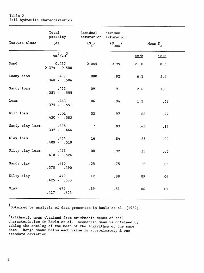
Table 2.

Soil hydraulic characteristics

Total Residual Maximum

porosity saturation saturation

Texture class (<f>) (S )r

(S )max

Mean Ks

cm3, 3. /cm cm/h in/h

Sand 0

0.374

.437

- 0.500

0.045 0.95 21.0 8.3

Loamy sand

.368

.437

- .506

.080 .92 6.1 2.4

Sandy loam.351

.453

- .555

.09 .91 2.6 1.0

Loam

.375

.463

- .551

.06 .94 1.3 .52

Silt loam

.420

.501

- .582

.03 .97 .68 .27

Sandy clay loam

.332

.398

- .464

.17 .83 .43 .17

Clay loam.409

.464

- .519

.16 .84 .23 .09

Silty clay loam

.418

.471

- .524

.08 .92 .15 .06

Sandy clay.370

.430

- .490

.25 .75 .12 .05

Silty clay.425

.479

- .533

.12 .88 .09 .04

Clay.427

.475

- .523

.19 .81 .06 .02

Obtained by analysis of data presented in Rawls et al. (1982)

2Arithmetic mean obtained from arithmetic means of soilcharacteristics in Rawls et al. Geometric mean is obtained bytaking the antilog of the mean of the logarithms of the samedata. Range shown below each value is approximately ± onestandard deviation.

G1

Arithmetic Geometric Arithmetic2

Geometric

cm cm in in

10.1 4.6 4.0 1.8

2.2 - 20.7 1.0 - 27.1 0.86 - 8.2 0.34 - 10.7

14.7 6.3 5.8 2.5

4.1 - 32.3 2.3 - 31.7 1.6 - 12.7 .91 - 12.5

24.8 12.7 9.8 5.0

9.8 - 52.6 3.0 - 54.0 3.6 - 20.7 1.2 - 21.3

37.5 10.8 14.8 4.3

18.5 - 93.7 1.9 - 74.0 7.3 - 36.9 .75 - 29.1

48.5 20.3 19.1 8.0

22.0 - 104.3 4.3 - :L18.0 8.7 - 41.7 1.7 - 46.5

61.7 26.3 20.1 10.422.0 - 107.0 6.0 - 132.0 8.7 - 42.1 2.5 - 52.0

53.3 25.9 21.0 10.225.0 - 117.4 6.7 - 116.0 9.8 - 46.2 2.6 - 45.6

72.0 34.5 28.3 13.637.0 - 147.0 8.5 - 168.0 14.6 - 57.9 3.3 - 66.1

76.8 30.2 30.2 11.937.3 - 173.0 5.6 - 178.0 14.7 - 68.1 2.2 - 70.1

81.2 37.5 32.0 14.843.0 - 170.0 9.3 - 182.0 16.9 - 66.9 3.7 - 71.7

89.0 40.7 35.0 16.046.0 - 183.0 8.8 - 204.0 18.1 - 72.0 3.5 - 80.3

10

which is the difference between the volumetric water-holdingcapacity of the soil and its initial water content. Callingthis parameter B, we have

B = G (8s - 8±) [3]

or

B = G <f> (S - S.) [3a]Y x max l

in which <f> is soil porosity, 8 and 8. are saturated and initial

3 3water contents [L /L 1, and S and S, are maximum and initial

1 ' J max i

values of relative saturation, defined as 8/<f>. Parameter B hasunits of length like G and simply combines the parameter G withthe time-dependent variable 8. or S.. In KINEROS we use the

second of these two expressions, since conceptually relativesaturation is easier to deal with as a value from 0 to 1.

Actually S, is limited on the lower end by the value of residual

saturation (S ). Values of S are presented in table 2 and

relative saturation values at permanent wilting point and "fieldcapacity" are shown in table 3 as an aid to judgment inselecting S..

Table 3.

Relative saturation at permanent wilting pointand field capacity

Relative saturation

Texture class Permanent wilting Field capacity

Sand 0.08 0.21

Loamy sand .13 .29Sandy loam .21 .46Loam .25 .58

Silt loam .27 .66

Sandy clay loam .37 .64Clay loam .42 .69Silty clay loam .44 .78Sandy clay .56 .79Silty clay .52 .81Clay .57 .83

Derived from mean values of Table 2 in

Rawls et al. (1982) using total porosity,

The infiltration expression used in KINEROS comes from Smith andParlange (1978):

Kg exp(F/B)/[exp(F/B)-l] 'M

The parameter K acts somewhat as a scaling parameter for f as

equation [4] indicates. For a short time interval after thebeginning of rainfall or small values of F (generally when F/B <0.1), equation [4] approaches the gravity-free infiltrationrelation

f = BK /Fc s'

[s:

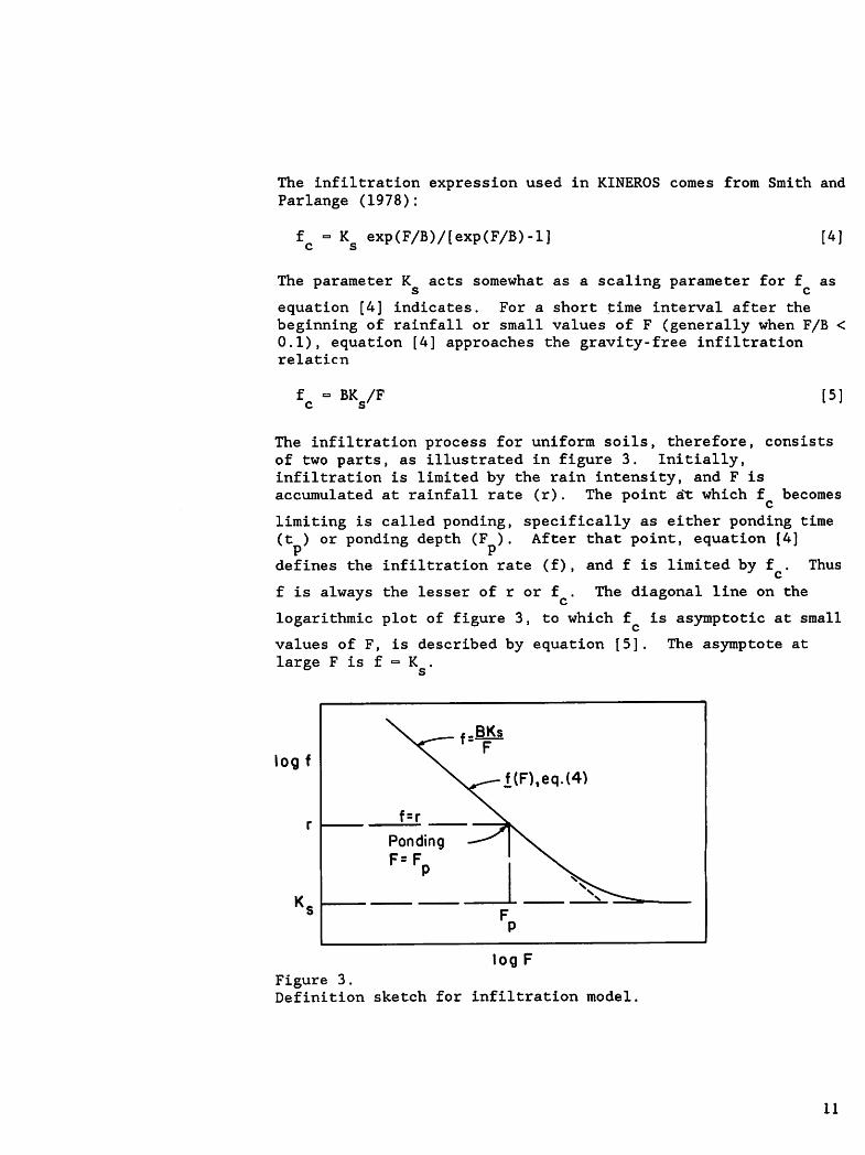
The infiltration process for uniform soils, therefore, consistsof two parts, as illustrated in figure 3. Initially,infiltration is limited by the rain intensity, and F isaccumulated at rainfall rate (r) . The point a*t which f becomes

r c

limiting is called ponding, specifically as either ponding time(t ) or ponding depth (F ). After that point, equation [4]

defines the infiltration rate (f), and f is limited by f . Thus

f is always the lesser of r or f . The diagonal line on the

logarithmic plot of figure 3, to which f is asymptotic at small

values of F, is described by equation [5]. The asymptote atlarge F is f =• K .

log f

. f-BKsT" F

\sr-f(F),eq.(4)

f=r

Ponding

f=fp

PF

logF

Figure 3.Definition sketch for infiltration model

11

12

Infiltration During Recession

When the rain ceases or falls to a rate below the infiltration

capacity (f ), infiltration continues from the rain and flowing

water still on the soil surface until the water is locallydepleted. Unlike rainfall, however, the supply of infiltratingwater from flowing water cannot reasonably be assumed to becontinuous over the surface. The kinematic treatment of the

surface water flow does not require the assumption of "sheet"flow. On natural surfaces, flows are commonly confined torivulets according to the geometry of the microtopography. As aresult, infiltration of surface water during recession islimited by the fraction of the soil surface exposed to thesurface water.

KINEROS provides a simple modification of infiltration duringrecession by describing the surface microtopography with aparameter RECS. This parameter represents, conceptually, thelocal maximum average depth of surface water flow for which thesurface is essentially completely covered by the water. Asaverage flowing water depth (h) is reduced below this depth,the surface covered by the flowing water is assumed to declinein direct proportion to the depth. Thus when the local meandepth is half of RECS, the soil surface is assumed to be halfcovered by the flowing water. A very low value of RECSrepresents a relatively smooth soil surface, with littletopographic variation, such as a sod-covered plane; a largevalue of RECS represents a very rough or rilled surface, withflowing water confined to a small part of the surface. Theratio of h to RECS is used to reduce the net rate of loss of

surface water by infiltration during recession conditions, asfar as the surface water flow equations are concerned.

Recovery of Infiltration Capacity During Rainfall Hiatus

The theory represented in equations [2] through [4] applies ingeneral when r > K . Often in real rainfall patterns there are

one or more intervals during a storm in which 0 < r < K . As

long as water remains on the surface to satisfy f , these

intervals are still covered by this theory.

When a longer hiatus occurs, in which part or all of the surfaceis free of water, redistribution of soil water will occur and asubsequent rainfall will find a new and larger value of S.. In

KINEROS, the changes in relative saturation during such aninterval are based on an analytic estimate of the water contentthat the soil would attain for a given r < K if that rainfall

° s

continued indefinitely. This steady unsaturated flowrelationship is based on a relation used by Brooks and Corey(1964) and others, between soil flux (equal to rain rate at alarge time) and relative saturation at the steady rate, S(r):

fcfS<r> = Sr + (Smax "V F" ; (r < V [6]

S and S are as defined previously, and p is an exponent onmax r

the order of 0.20. The long term S(r) is not achieved in thecontext of a typical changing pattern of r but is useful forestimating the direction of change of S.. If rain rate

increases from 0 to r. (r. < K ), water content will increaseJ J s

toward S(r.) (equation [6]). Neglecting surface evaporation,

the long term value of relative saturation for r - 0 is S .

KINEROS estimates the change of S. during a hiatus by assuming

this value moves asymptotically toward the value of S(r) as longas r < K :

s

Si ~Si_1 +[min (S" Sc) "Si |i1 "exP(-^At)| ^in which j superscript or subscript represents time levels, andi) is a rate factor which we wish to be a function of the depthof water previously infiltrated, and also a function of theamount of water still on the surface:

[1 - h/RECS]exp(-2F)JaK [8;s

S is the relative saturation at field capacity (-0.33 bars) asc

computed from a non-linear regression relationship derived frommean values of K versus water content at field capacity from

s

Rawls et al. (1982). S is computed from the regression

relationship using the input K so the user does not need to

supply this quantity.

For a long hiatus equation [8] tends toward the initial relative

(S.) if ST < S and tends toward relative field capacity (S ) ifv i7 l c c

s] > S .l c

13

14

This is a conceptual relation, but it has worked adequatelybased on experimental data from Walnut Gulch watershed inArizona. The relationship provides that redistribution proceedsmore slowly for large rains (F) or for tighter soils (low K ),

and more rapidly for small F or large K . "a" is a fitting

parameter, and is currently set to 0.95. RECS was definedpreviously, and the first term in this expression provides forthe reduced redistribution rate when water partly covers thesurface during recessions.

Numerical Treatment

In the context of a simulation model, solution of many equationsmoves forward in time steps, and one needs to know theconditions during each step. In the case of infiltration, weneed a value for the mean infiltration rate over the time stepat every location along the flow path. When the solution mustproceed in the time domain, an approach is required that variesfrom the straightforward application of the previous equations.

Recognizing that f - dF/dt, one may write dF/dt = f(F) andintegrate this relation in steps:

At -

F(t)

F(t + At)

dF

f(F)[9

The true mean value of f over an interval from time t to t + Atc

(with f less than r) is obtained as

f(At) - AF/At - [F(t + At) - F(t)]/(At) [10]

F(t + At) is obtained numerically using equation [9] over the

interval At divided into as many increments as desired. Theinfiltration rate (f(F)) in equation [9] is taken along the linef = r for up to ponding depth and then follows f(F) fromequation [4], as in figure 3.

Equation [4] is also used to calculate infiltration fromtrapezoidal channels. It is applied at each computational nodeover an area equal to the product of the effective wettedperimeter and the length increment (Ax), and becomes part of thelateral inflow term (see equation [23]).

Hortonian Overland

Flow

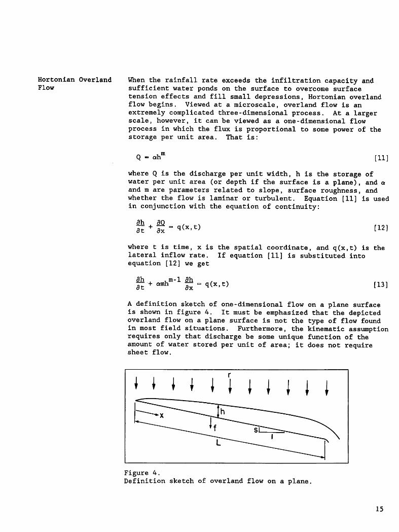
When the rainfall rate exceeds the infiltration capacity andsufficient water ponds on the surface to overcome surfacetension effects and fill small depressions, Hortonian overlandflow begins. Viewed at a microscale, overland flow is anextremely complicated three-dimensional process. At a largerscale, however, it can be viewed as a one-dimensional flowprocess in which the flux is proportional to some power of thestorage per unit area. That is:

mah 11

where Q is the discharge per unit width, h is the storage ofwater per unit area (or depth if the surface is a plane), and aand m are parameters related to slope, surface roughness, andwhether the flow is laminar or turbulent. Equation [11] is usedin conjunction with the equation of continuity:

3h dQ3t 3x

q(x,t) [12]

where t is time, x is the spatial coordinate, and q(x,t) is thelateral inflow rate. If equation [11] is substituted intoequation [12] we get

3h , ,m-l ahfl + amn —at 3x

= q(x,t) [13!

A definition sketch of one-dimensional flow on a plane surfaceis shown in figure 4. It must be emphasized that the depictedoverland flow on a plane surface is not the type of flow foundin most field situations. Furthermore, the kinematic assumptionrequires only that discharge be some unique function of theamount of water stored per unit of area; it does not requiresheet flow.

Figure 4.Definition sketch of overland flow on a plane

15

16

The kinematic wave equations are a simplification of thede Saint Venant equations and do not preserve all the propertiesof the more complex equations. Specifically, backwater cannotbe accommodated and waves do not attenuate (unless they formshocks that do attenuate). It has been shown that the kinematicwave formulation is an excellent approximation for most overlandflow conditions (Woolhiser and Liggett 1967, Morris andWoolhiser 1980).

The depth at the upstream boundary must be specified to solvethe kinematic wave equations. If the plane is the uppermostone, the appropriate boundary condition is

h(0,t) - 0 :i4]

If another plane is contributing runoff to the upper boundary ofthe plane in question, the boundary condition is

h(0,t)

mu

[ ot h (L,t)L u u

Wu /( a W ) ]1/m

where h (L,t) is the depth at the lower boundary of theu

contributing plane at time t, W is the width of theu

[is:

contributing plane, a is the slope-roughness parameter for theu

contributing plane, m is the exponent for the contributingu

plane, and a, m, and W refer to the lower or receiving plane.

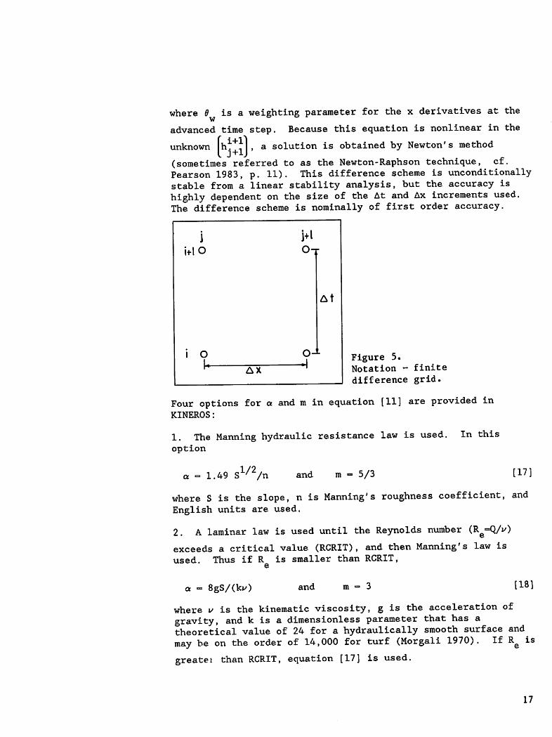
In KINEROS the kinematic wave equations are solved numericallyby a four-point implicit method. Notation for the finite-difference grid is shown in figure 5 and the finite-differenceequation is

i+1

lj+l

2At

Ax

i+1

*J+1 + *j

•j# <**>;;; --r«n

«-•-> [-u <hm> ;+1- -i <hm> ]]'

"At (vi +*J 16

where 8 is a weighting parameter for the x derivatives at the

advanced time step. Because this equation is nonlinear in the

unknown [hV"-I ,asolution is obtained by Newton's method(sometimes referred to as the Newton-Raphson technique, cf.Pearson 1983, p. 11). This difference scheme is unconditionallystable from a linear stability analysis, but the accuracy ishighly dependent on the size of the At and Ax increments used.The difference scheme is nominally of first order accuracy.

J

i*lo

O

AX

At

o-t--I

Figure 5.Notation - finite

difference grid.

Four options for a and m in equation [11] are provided inKINEROS:

1. The Manning hydraulic resistance law is used. In thisoption

1.49 S1/2/ri and m 5/3 [17

where S is the slope, n is Manning's roughness coefficient, andEnglish units are used.

2. A laminar law is used until the Reynolds number (Re=Q/V)exceeds a critical value (RCRIT), and then Manning's law isused. Thus if R is smaller than RCRIT,

e

a - 8gS/(kv) and m •= 3 [18]

where v is the kinematic viscosity, g is the acceleration ofgravity, and k is a dimensionless parameter that has atheoretical value of 24 for a hydraulically smooth surface andmay be on the order of 14,000 for turf (Morgali 1970). If R& is

greatei than RCRIT, equation [17] is used.

17

18

3. A laminar law is used until the Reynolds number exceeds acritical value and then the Chezy law is used. Thus if R is

e

smaller than RCRIT, equation [18] is used. If R is greater

than RCRIT,

a -CS1//2 and m- 3/2 [19]

where C is the Chezy friction coefficient.

4. The Chezy law, equation [19] , is used for all values of Re

Overland flow response characteristics are controlled by theslope, slope length, and hydraulic resistance parameters as wellas the rainfall intensity and infiltration characteristics. Forexample, if the Manning resistance law is used, the time toequilibrium (tg) of a plane of length (L) and slope (S) with aconstant rate of lateral inflow (q), is

3/5

te

n L

1.49S1/2 2/3 [20:

where n is the Manning resistance coefficient. Therefore, tomaintain the time response characteristics of the catchment wemust retain the slope, slope length, and hydraulic resistance inour simplified version of a complex catchment. The length,width, and slope of the plane elements can be determined fromtopographic maps. The hydraulic resistance (or parameter) ismore difficult to determine. First, a decision must be maderegarding the appropriate flow law. It is generally agreed thatoverland flow on a plane begins as laminar flow and eventuallybecomes turbulent at large Reynolds numbers. Values of thecritical Reynolds number range from 100 to 1,000 (Chow 1959, Yuand McNown 1964, Morgali 1970). However, raindrops impacting onthe water film generate local areas of turbulent flow and havean effect similar to increasing the viscosity of the fluid. Forexample, the relationship between the Darcy-Weisbach frictionfactor (fQ) and Reynolds number for laminar flow over ahydraulically smooth surface is

- 24

fD - r t21J

Several laboratory experiments (cf. Glass and Smerdon 1967, Li1972) have shown that with raindrop impact this relationshipbecomes

f^ - k/R ; k > 24 [22]D ' e

k - k + f(r) [22a]o

where k is the appropriate value for a given surface geometry

without raindrop impact and f(r) is some function of therainfall rate. Although the effects of raindrop impact can besignificant on hydraulically smooth surfaces such as laboratorycatchments, they are not important for hydraulically roughsurfaces usually found in the field. The laminar flow model inKINEROS does not include a relationship between k and rainfallrate. Ranges of k for various surfaces are presented in table

Although the range of k for each surface is large, the time of

1/3equilibrium is proportional to k ' , so a 10 percent error in

k will cause a smaller error in t . It should be noted thato e

the relationship R = Q/ = uh/ is used for all surfaces in

KINEROS although, for example, the local depth (h) may not bethe appropriate characteristic length to use in flow throughdense sod.

In KINEROS it is not necessary to specify the critical Reynoldsnumber; rather, the appropriate turbulent Manning's n or Chezy Cis chosen. This choice will define the critical Reynoldsnumber, which is then used in the program to change the frictionlaw at the appropriate time. Ranges of Manning's n and Chezy Cobtained from experiments reported in the literature are alsoshown in table 4, and values of Manning's n are shown for a widerange of surfaces in table 5. These values are generallyrepresentative of very small areas when correspondence existsbetween reality and the mathematical model of one-dimensionalflow over a plane. If a plane is used to represent areas largerthan about 2 acres (0.8 ha), these values should be adjusted (ndownward, C upward) to reflect the greater number of rills onlong slopes. Some guidance is available in the literatureregarding appropriate roughness adjustments and geometric modelsimplification. Refer to Lane et al. (1975), Lane and Woolhiser(1977), Wu et al. (1978), and Goodrich et al. (1988) forbackground information.

19

Table 4.

Resistance parameters for overland flow

Laminar flow (k )0

Turbulent flow

Surface Manning's n Chezy C

ft1'*,.

Concrete or asphalt 24 108 0.01 - 0.013 73 - 38

Bare sand 30 120 .01 - .016 65 - 33

Graveled surface 90 400 .012 - .03 38 - 18

Bare clay-loam soil 100 500 .012 - .033 36 - 16

(eroded)Sparse vegetation 1,000 - 4 ,000 .053 - .13 11 - 5

Short grass prairie 3,000 - 10 ,000 .10 - .20 6.5 - 3.6Bluegrass sod 7,000 - 40 ,000 .17 - .48 4.2 - 1.8

Source: Woolhiser (1975).

Channel Routing

We recommend that option 1, Manning's law, be used for KINEROSunless the watershed to be modeled is very small andhydraulically smooth, in which case option 2 (Laminar-Manning)is recommended. Options 3 and 4 are included for researchapplications.

Unsteady, free surface flow in channels is also represented bythe kinematic approximation to the equations of unsteady,gradually varied flow. Channel segments may receive uniformlydistributed but time-varying lateral inflow from planes oneither or both sides of the channel, or from one or two channelsat the upstream boundary, or from a plane at the upstreamboundary. The dimensions of planes are chosen to completelycover the watershed, so rainfall on the channel is notconsidered directly. The continuity equation for a channel withlateral inflow is

20

3A

at

2Qax

qc(x,t) 23

where A is the cross-sectional area, Q is the channel discharge,and qc(x,t) is the net lateral inflow per unit length of

channel. Under the kinematic assumption, Q can be expressed asa unique function of A and equation [23] can be written as

dk ^ dQ 3Aat dA ax nc 24

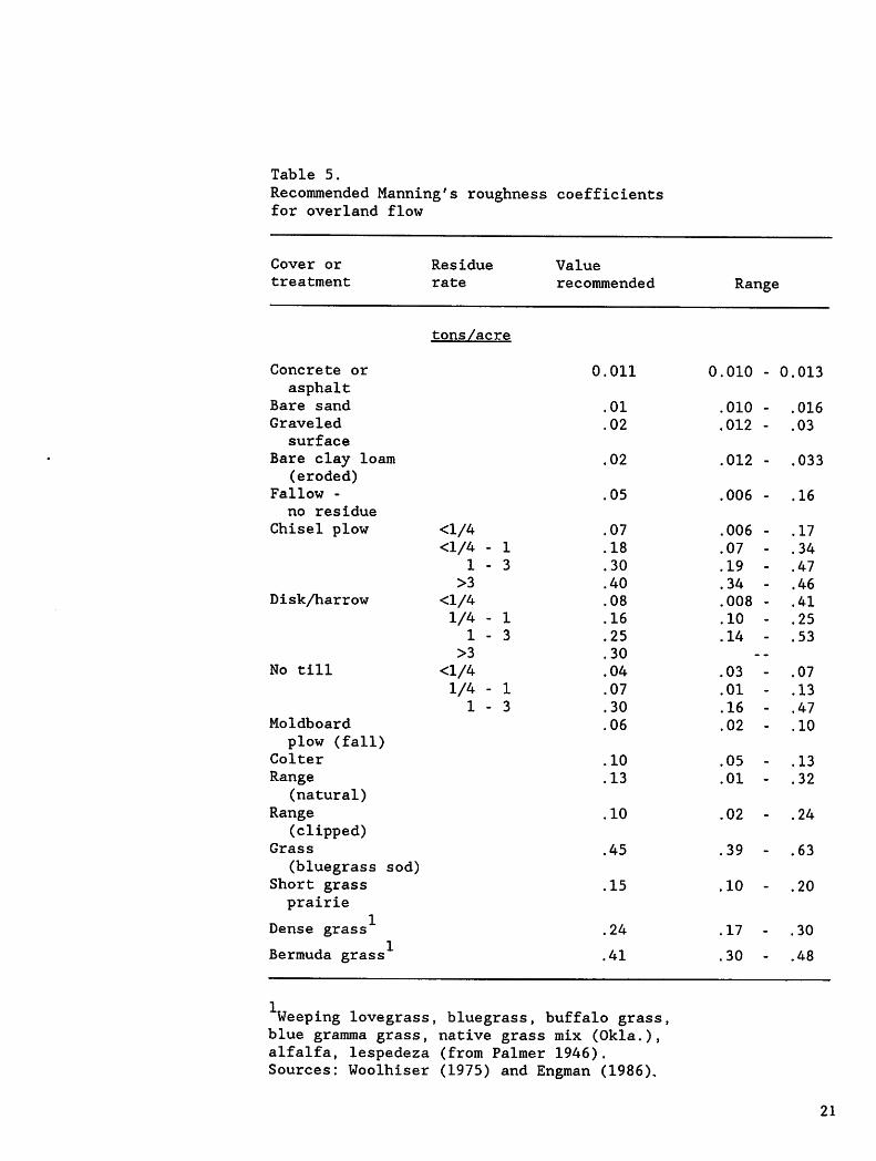
Table 5.

Recommended Manning's roughness coefficientsfor overland flow

Cover or

treatment

Concrete or

asphaltBare sand

Graveled

surface

Bare clay loam(eroded)

Fallow -

no residue

Chisel plow

Disk/harrow

No till

Moldboard

plow (fall)Colter

Range(natural)

Range

(clipped)Grass

(bluegrass sod)Short grass

prairie

Dense grass

Bermuda grass

Residue

rate

tons/acre

<l/4<l/4

1

>3

<l/41/4

1

>3

<l/41/4

1

Value

recommended

0.011

.01

.02

.02

.05

.07

.18

.30

.40

.08

.16

.25

.30

.04

.07

.30

.06

.10

.13

.10

.45

.15

.24

.41

Weeping lovegrass, bluegrass, buffalo grass,blue gramma grass, native grass mix (Okla.),alfalfa, lespedeza (from Palmer 1946).Sources: Woolhiser (1975) and Engman (1986).

Range

0.010 - 0.013

010 -

012 -

012 -

006 -

016

03

,033

,16

.006 - .17

.07 - .34

.19 - .47

.34 - .46

.008 - .41

.10 - .25

.14 - .53

.03 - .07

.01 - .13

.16 - .47

.02 - .10

.05 - .13

.01 - .32

.02 - .24

.39 - .63

.10 - .20

.17 - .30

.30 - .48

21

22

The kinematic assumption is embodied in the relationship betweenchannel discharge and cross-sectional area.

aR A [25

where R is the hydraulic radius. If the Chezy relationship is

used, o = CjS and m = 3/2. If the Manning equation is used, a1/2

1.49S ' /n and m = 5/3. Channel cross sections may beapproximated as trapezoidal or circular, as shown in figure 6.Equations for various functions of trapezoidal geometry areshown in table 6.

\ /

ZL|\l.0\

i

' /zizR (§j; h D

>

\BW ,

V Channel conduit

Trapezoidal cha nnel

Figure 6.Channel and conduit cross sections.

In an urban environment, circular conduits must be used torepresent storm sewers. For the kinematic model to apply, theremust be no backwater and the conduit is assumed to maintain free

surface flow conditions at all times--there can be no

pressurization. The continuity equation for a circular conduitis the same as equation [23] with q 0 That is, there is no

lateral inflow. The upper boundary condition is a specifieddischarge as a function of time. The most general dischargerelationship and the one often used for flow in pipes is theDarcy-Weisbach formula:

fn 2

where S_ is the friction slope, f is the Darcy-Weisbach

friction factor, and u is the velocity (Q/A). Under the

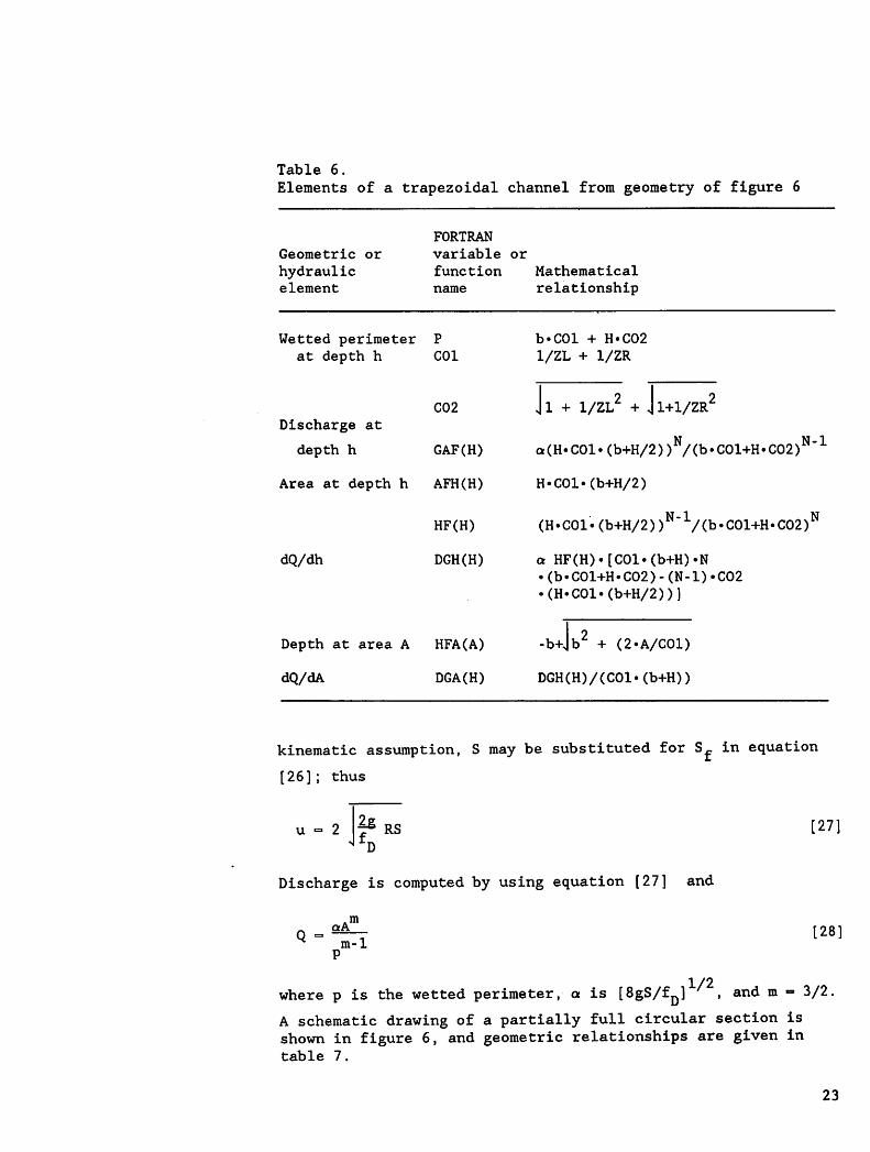
Table 6.lauxe o.

Elements of a trapezoidal channel from geometry of figure 6

Geometric or

hydraulicelement

FORTRAN

variable or

function Mathematical

name relationship

Wetted perimeter Pat depth h C01

Discharge at

depth h

dQ/dh

C02

GAF(H)

Area at depth h AFH(H)

HF(H)

DGH(H)

Depth at area A HFA(A)

dQ/dA DGA(H)

b-C01 + H-C02

1/ZL + 1/ZR

J1 +1/ZL2 +J1+1/ZR2

a(H.COl.(b+H/2))N/(b.C01+H.C02)N"1

H«C01«(b+H/2)

(H^C01.(b+H/2))N'1/(b«C01+H«C02)N

a HF(H)»[C01«(b+H)»N•(b.C01+H.C02)-(N-l)«C02•(H»C01.(b+H/2))]

hjb2 + (2«i•b+Jb + (2»A/C01)

DGH(H)/(C01«(b+H))

kinematic assumption, S may be substituted for Sf in equation

[26]; thus

u2g

JfTRS [27]

Discharge is computed by using equation [27] and

aAm

m-1[28:

1/2where p is the wetted perimeter, a is [8gS/fD] , and m = 3/2A schematic drawing of a partially full circular section isshown in figure 6, and geometric relationships are given intable 7.

23

24

Table 7.

Geometric elements of a partially full circularconduit from geometry of figure 6

Element

Depth (h)

Area (A)

Hydraulic radius (R)

Wetted perimeter (p)

Hydraulic depth (h_)

Relationship

D[l -cos (*c/2)]/2

D [0 - sin0 1/8

D(l - sin8c/8cyu

D^J/2

'8 - sinflc c

sin5 /2c'

/8

The kinematic equations for channels are solved by a four pointimplicit technique:

A1^ -A* +Ai+1 -A1 +2fj+1 j+1 J j Ax

+ (1-v [£[*U •*})

w

dQ1+1[ .i+1dA («js •«r

n ca^ f 1+1 1+1 1 1 1 A0.5At q .., + q 4 + q • , •, + q • =0^ Mcj+1 Mcj Mcj+1 X) J29

where 0 is a weighting factor for the space derivative.

Newton's iterative technique is used to solve for the unknown

area A - . The finite difference equation for circular

conduits is the same as equation [29] except that the lateralinflow terms (q ) are zero,

^c

The appropriate value of Manning's n or Chezy C to use forchannels in KINEROS depends on (1) the channel material (thatis, grassed waterway, gravel bedded stream, concrete-linedchannel), (2) the degree to which the channel conforms to theidealized trapezoidal cross section, and (3) how straight thechannel reach is. Because of these factors, choice of theappropriate parameters is highly subjective, except forartificial channels. Barnes (1967) estimated Manning's n forseveral streams and presented pictures of the stream reaches.These photographs are very useful in obtaining estimates fornatural channels. Values of Manning's n or Chezy C forartificial channels can be obtained from several sources,including Chow (1959).

In arid and semiarid regions, infiltration into channel alluviummay significantly affect runoff volumes and peak discharge. Ifthe channel infiltration option is selected, the integrated formof equation [4] is used to calculate accumulated infiltration ateach computational node, beginning either when lateral inflowbegins or when an advancing front has reached that computationalnode. Because the trapezoidal channel simplification introducessignificant error in the area of channel covered by water at lowflow rates (Unkrich and Osborn 1987), an empirical expression isused to estimate an "effective wetted perimeter." The equationused in KINEROS is

p = mmre

h/(0.15jBW), 1.0 p [30:

where p is the effective wetted perimeter for infiltration, h

is the depth, BW is the bottom width, and p is the channelwetted perimeter at depth h. This equation states that p is

smaller than p until a threshold depth is reached, and at depthsgreater than the threshold depth, p and p are identical. The

channel loss rate is obtained by multiplying the infiltrationrate by the effective wetted perimeter. Further experience maysuggest changes in the form and parameters of equation [30].

Reservoir Routing In addition to surface and channel elements, a watershed maycontain up to three reservoir elements, which receive inflowfrom one or two channels and produce outflow from anuncontrolled outlet structure. Rain falling on the pond andinfiltration from the pond are not considered. As long asoutflow is solely a function of reservoir depth, the reservoiris well described by the mass balance and outflow equations:

dt " «I " q0 [31]

25

Erosion and Sediment

Transport

26

and

*0C.(h1 r V

in which V = V(h ) is reservoir volume [L ],

h « reservoir surface elevation [L],

q = inflow rate [L /T],

3q = outflow rate [L /T],

h = reservoir outflow weir elevation [L], andz

C and c. weir coefficients

[32]

Reservoir surface elevation (h ) is measured from some datumr

below the lowest pond elevation, and V(h ) is determined from

the description of the reservoir geometry. Equation [31] iswritten in finite difference form over a time interval (At) andthe stage at time t + At is determined by the bisection method.

For purposes of water routing, the reservoir geometry may bedescribed by a simple relation between V and h . However, one

of the functions of reservoirs may be to trap sediment, so amore complete description is required by KINEROS. The reservoiris described as a survey would characterize it, with a series ofcross sections using a common base elevation. An example isshown in figure 7. The cross sections are assumed to be normalto the flow of water through the reservoir, starting at theinput end and ending at the outflow structure. Knowledge offlow cross-section changes along the flow path through thereservoir is important in routing the deposition of sediment inthe pond. The description of the shape of the reservoir isconverted within the program into a V(h ) relation for use in

the previous equations.

As an optional feature, KINEROS can simulate the movement oferoded soil along with the movement of surface water. KINEROSaccounts separately for erosion caused by raindrop energy anderosion caused by flowing water. Similar procedures are used todescribe transport of sediment within surface and channelelements. Transport of sediment through a reservoir element ishandled very much like the analogous process in a settling pond.

El MO

108

El 110-

I08:

El 110-

108:

106'

"^^7"

s

ss: 2

z_

« TWP (D.4)El M0-

108-

106-

za

^^^^^E

El 110-

108-

106^

5Ss:

ELZQ

•AP(D,4)

^ S F MEL=6

<* .S

ELVZ

Figure 7.Pond geometry for KINEROS

Upland Erosion

Weir

NSEC=6

The general equation used in KINEROS to describe the sedimentdynamics at any point along a surface flow path is a massbalance equation similar to that for kinematic water flow(Bennett 1974):

fc(AC.) +fx"(QCs) "e(x't) -V*^3 3

in which C = sediment concentration [L /L ],

cross sectional area of flow [L ],2

rate of erosion of the soil bed [L /T], andrate of lateral sediment inflow for channels

[L /T/L].

[33:

27

28

For upland surfaces, e is assumed to be composed of two majorcomponents--production of eroded soil by splash of rainfall onbare soil and hydraulic erosion (or deposition) due to theinterplay between shear force of water on the loose soil bed andthe tendency of soil particles to settle under the force ofgravity. Referring to splash erosion rate as g and hydraulic

erosion rate as g, , we have

e = fes + gh [34]

Based on limited experimental evidence, splash erosion rate canbe approximated as a function of the square of the rainfall rate(Meyer and Wischmeier 1969). We have found that thisrelationship can lead to physically unrealistic concentrationsat the upstream boundary, so in KINEROS we use the followingrelation:

gg - cfk(h)rq; q > 0 [35]

=0; q < 0

in which c_ is a constant and k(h) is a reduction factor

representing the reduction in splash erosion caused byincreasing depth of water. It is 1.0 prior to runoff and itsminimum is 0 for very deep flow. The function k(h) is given bythe empirical expression

k(h) - exp (-chh) [36]

Both c_ and k(h) are always positive, so g is always positive

when there is rainfall and a positive rainfall excess (q). Onthe other hand, g, represents the rate of exchange of sediment

between the flowing water and the soil over which it flows, andmay be either positive or negative. KINEROS assumes that forany given surface water flow condition (velocity, depth, slope,etc.), there is an equilibrium concentration of sediment thatcan be carried if that flow continues steadily. Hydraulicerosion rate (g, ) is estimated as being linearly dependent on

the difference between the equilibrium concentration and thecurrent sediment concentration. In other words, hydraulicerosion is modeled as a kinetic transfer process:

g, = c (C - C )A [371°h g mx s l J

in which C is the concentration at equilibrium transportmx

capacity, C = C (x,t) is the current local sediment

concentration, and c is a transfer rate coeffficient [T ].o

Clearly the transport capacity is important in determininghydraulic erosion, as is the selection of transfer ratecoefficient. Conceptually, c would be very low for cohesive

material and very high (realistically, less than 0.1 s ) forfine, totally noncohesive material. Foster et al. (1983)proposed a function to estimate c based on the Universal Soil

Loss Equation (USLE) (Wischmeier and Smith 1965 1978) soilerodibility factor plus information on the soil mulch andresidue conditions. This method is applicable to cultivatedsoils and may be used in KINEROS.

Many transport capacity relations have been proposed in theliterature, but most have been developed and tested forrelatively deep, mildly sloping flow conditions, such as streamsand flumes. In the absence of a clearly superior relation forshallow surface runoff, KINEROS provides the user a choicebetween several transport relationships: (1) A "tractive force"relation used by Meyer and Wischmeier (1969) and attributed toLaursen (1958), (2) the unit stream power relation of Yang(1973), (3) the Bagnold relationship (Kilinc and Richardson1973), (4) the relation from Ackers and White (1973), (5) thetransport relation of Yalin (1963), and (6) the transportrelation of Engelund and Hansen (1967). These relations havebeen studied and compared by Alonso et al. (1981) and by Julienand Simons (1985), who showed that each could be represented bya generalized relation of the type

q = C Q= o> S^ Q7 r6nm mx

1 - ; t > ro c

2 -1in which q = transport capacity [L T ],

38

r = bed shear stress [L /T],o

2r = critical shear stress [L /T], andc

w = a coefficient.

Exponents /J, 7, and e have values of either 0 or between 1 and2, and 6 varies from 0 to -2.24. The equations for eachtransport relationship are presented in the appendix.

29

30

Although not every transport relation selectable in KINEROS hasnon-zero values for all the exponents /9, 7, and e, all use suchlocal hydraulic conditions as slope, velocity, or depth of flow.Some, in addition, use sediment specific gravity and the meanparticle size of the soil rather than requiring selection of anempirical coefficient.

The hydraulic erosion parameter (c ) has two interpretations.

It represents erodibility as constrained by cohesiveness andrelated factors when C is greater than C . Alternatively, c

mx ° s gis a function of the relative fall velocity of the median size

particles when deposition is occurring, that is, when C exceeds

C .mx

In local deposition, the value of c is calculated from particleg

size and density. Particle fall velocity (v ) may be calculated

from particle density and size, assuming the particles have dragcharacteristics and terminal fall velocities similar to those of

spheres (Fair and Geyer 1954):

2 4 g(Ss - 1)d\ - 3̂ t39'-2

in which g = gravitational acceleration [LT ],S = particle specific gravity,

C = drag coefficient, and

d = particle diameter [L].

The drag coefficient is a function of particle Reynolds numberas follows:

n n

in which R is the particle Reynolds number, defined as

R - v d/v [41]n s ' l J

2where u is kinematic viscosity of water [L /T]. Settlingvelocity of a particle is found by solving equations [39], [40],and [41] for v . The coefficient c in equation [37] is then

1 J s g

vs

c (deposition) = ~g h

D

Cmx

Cs

42

where h is the hydraulic depth.

In physical terms, this expression says that the particles inexcess of the carrying capacity concentration (C ) will be

removed at the settling velocity rate.

Numerical Solution

Equation [33] is solved numerically at each time step used bythe surface water flow equations. A four-point implicit finite-difference scheme is used; however, iteration is not required iferosion is occurring since given current and immediate pastvalues for A and Q and previous values for C , the finite-

difference form of this equation can be solved for C . , as as j+1

function of C ., C . - , and Cs j s j+1' s j

During deposition the values of C and C in equation [42] are° mx s i i j

taken as C ... and C .-so iteration is not required,mx j+1 s j+1 n

When runoff commences during a period when rainfall is creatingsplash erosion, the initial condition on the vector C should

not be taken as zero. The initial sediment concentration at

ponding (C (t=t )), can be found by simplifying equation [33]s p

for conditions at that time. Variation with respect to xvanishes, and hydraulic erosion is zero. We may then state

|j (ACg) -e(x,t) -cfrq [43]

Here we have assumed k(h) =1.0 since depth is zero. If weexpand the derivative and note that A is zero at time of pondingand recognize that dA/dt is the rainfall excess rate (q), wefind

c r q

c (t=t >" r\ s l44ls p (q+v )

The sediment concentration at the upper boundary of a singleplane

[44].

plane C (0,t) is given by an expression identical to equation

31

32

Channel Erosion and Sediment Transport

The general approach to sediment transport simulation forchannels is nearly the same as that for upland areas. The majordifference in the equations is that splash erosion (gg) is

neglected in channel flow, and the term q becomes important in

representing lateral inflows. Equation [33] is equallyapplicable to either channel or distributed surface flow. Thechoice of transport capacity relation may be different for thetwo flow conditions. For upland areas, q will be zero, whereas

for channels it will be the important addition that comes withlateral inflow from surface elements. The close similarity ofthe treatment of the two types of elements allows the program touse the same algorithms for both types of elements.

The computational scheme for any element uses the same time andspace steps employed by the numerical solution of the surfacewater flow equations. In that context, equation [33] is solvedfor C (x,t), starting at the first node below the upstream

boundary, and from the upstream conditions for channel elements.If there is no inflow at the upper end of the channel thetransport capacity at the upper node is zero and the depositionmode is in effect. The upper boundary condition is then

V0^ -q+"' BW [45]nc s

where BW is the channel bottom width.

Note that for a triangular channel the upper boundary concentration is equal to the concentration in the lateral inflow.A(x,t) and Q(x,t) are assumed known from the surface watersolution.

Sediment Routing Through Reservoirs

For shallow rapid flow where erosion is generally more importantthan deposition, the use of a mean particle diameter can usuallybe justified for simulation purposes. When reservoirs areimportant elements in the catchment, however, KINEROS asks theuser to specify a particle size distribution, because depositionis the only sedimentation process, and settling velocity is verysensitive to particle size. The distribution is characterizedby a mean and a standard deviation and is assumed pseudonormallydistributed into particle size classes as specified by the user.

As indicated, the approach for pond sedimentation in KINEROS issimilar to that for tank sedimentation, and particle fallvelocities and flow-through velocities are used to find thetrajectories that intersect the reservoir bottom. The inputreservoir cross sections describe its shape (see fig. 7)successively from the inlet to outlet ends of the reservoir.Particle fall velocities are calculated for each particle sizeclass using equations [39] - [41]. Particles are assumeddistributed uniformly through the reservoir depth in the firstsection at the inlet end, and the relative fall versus lateralvelocities from that point forward determine the proportion ofeach particle size class that deposits between successive crosssections. At successive sections, each particle size class willhave a conceptual depth from the surface to the top of the areastill containing sediment of that size.

Suspended and slowly falling particles are subject to moleculardiffusion and dispersion, which can sometimes modify the timedistribution of outflow concentrations. KINEROS simulates thismodification using an effective dispersion coefficient, which is

supplied by the user. Typical values suggested are from 10 to

10 ft /s. In many cases, dispersion is unimportant and can beneglected, such as for very short flow-through situations or forlarge particles.

If a pond is located within a watershed, the mean particlediameter of the outflow will be smaller than that of the inflow.KINEROS cannot account for this phenomona.

Since the time necessary for a reservoir outflow to approachzero may be significantly longer than that for a channel inputhydrograph to return to zero, the user may need to specify amuch longer simulation time if a pond or ponds are included inthe catchment geometry.

33

KINEROS PROGRAM DOCUMENTATION

Program Description A FORTRAN77 program has been written to implement the KINEROSmodel. The code is structured, with 42 subroutines orfunctions, each performing specific model functions. Table 8lists the subroutines and defines their tasks.

KINEROS is run interactively, with the program prompting theuser for names of input and output files. When files are usedrepetitively (for example, on initial runs where parameters arevaried for purposes of "calibration"), the user has the optionto reuse files without having to reenter the names.

Two input files (or additional files for PONDS) are required torun KINEROS and two output files are always written. Detailedfile descriptions follow. It is suggested that the user followa file-naming convention to simplify KINEROS usage. Thedevelopers typically call input parameter files by a name thatdescribes the location and watershed with the extension .PAR,for example, LUCKY103.PAR for Lucky Hills Watershed 103parameter file. Similarly, LUCKY103.PRE would be theprecipitation file for that location. Some users incorporatethe rain dates in the file names. LUCKY103.DAT would be thestandard hydrologic output, and LUCKY103.AUX is the auxiliarydetailed output. KINEROS makes no demands of the user so far asfile names are concerned. A naming convention is recommendedsimply for easy use.

The developers have experienced the frustrations of handlinginput files consisting of matrices of unidentified numbers,where one changes the watershed area when intending to change achannel length. Because FORTRAN77 does not support the handyNAMELIST function, KINEROS input files have been constructed astemplates, with each variable's name appearing above the spacewhere the value should be entered and with some guidance as toline duplication requirements where necessary. Sample templatefiles are illustrated with run examples in the next section andare included on the program diskette.

34

Table 8.

KINEROS program and subroutines

PROGRAM MAIN:

SUBROUTINES:

ADD:

BISECT:

CAPACY:

CHANINF:

CHANNL:

CHGLAW:

CONVERT:

DEFAULT:

ERROR:

FCP:

FINTG:

FOF:

Calls subroutines INTSEL, READER, PLANE, CHANNL, POND, CONVERTand HYDRITE

Adds specified discharges (lateral flow, channel junctions)and computes upstream boundary values (depth, area, orintersection angle 0 in conduits). Called from CHANNL and

POND. Calls ERROR, ITER, and GOTOER.

Locates the minimum of an external one-dimensional function

using the bisection method. Called from ITER. Calls FCT.

Calculates erosion transport capacity for local suspendedsediment concentration (equation [37]). Called from SEDCOM.Calls SHIELDF.

Calculates an index accumulated infiltration depth at eachnode using the integrated form of equation [4]. Called fromIMPLCT.

Implicit finite difference solution for unsteady flow inchannels with trapezoidal or circular cross sections. Calledfrom MAIN. Calls IMPLCT, SEDCOM, ADD, RESLAW, CHGLAW, andVSETL.

Changes the hydraulic resistance laws at the transitionReynolds number if Laminar-Turbulent option has been selected.Called from IMPLCT, CHANNL and PLANE.

Converts units of time and length in input data to units usedinternally and reconverts to desired units in output. Calledfrom MAIN and READER.

Sets default values for parameters. Called from PAREAD.

Prints appropriate execution error messages. Called fromREADER, PONDRD, ADD, PLANE, IMPLCT, and IMPAUB. Calls GOTOER.

Finds flux capacity as a function of water in soil profile.Called from FINTG and XPLINF.

Integrates infiltration equation [4]. Called from XPLINF.Utilizes functions QCP, FCP, and FOF.

Returns the cumulative infiltration depth. Called from FINTG,

35

Table 8--Continued.


GOTOER:

HOFV

HYDRITE:

IMPAUB:

IMPCHA:

IMPCIR:

IMPLCT:

IMPOCF:

IMTHUB:

INSPEC:

INTSEL:

ITER:

36

Escape routine called when arguments are incorrect in acomputed "GO TO" statement. Called from INSPEC, ERROR, ADD,RESLAW, PLANE, and IMPLCT.

Calculates pond surface elevation given surface area or volumeby log interpolation. Called from POND.

Writes hydrograph for selected element (plane or channel).Called from MAIN.

Calculates an error function for an assumed area in theiterative solution for the upper boundary area of atrapezoidal channel, given an upstream discharge. Called fromADD through ITER. Calls ERROR.

Calculates an error function for an assumed area in theiterative solution for cross sectional area in a trapezoidal

Called from IMPLCT through ITER.channel

Calculates an error function for assumed value of theindependent variable d in the iterative solution for cross

sectional area in a circular channelthrough ITER.

Called from IMPLCT

Four point implicit finite difference scheme. Called fromsubroutines PLANE and CHANNL. Calls ITER, CHGLAW, GOTOER,ERROR, and CHANINF.

Calculates an error function for an assumed depth h in theiterative solution of depth along a plane. Called from IMPLCTthrough ITER.

Calculates an error function for an assumed value of theindependent variable $c in the iterative solution of upperboundary area of a circular conduit, given an upstreamdischarge Q from ADD. Called from ADD through ITER.

Inspects input data for errors and prints out an error messageif one is detected. Called from READER and PAREAD. CallsERROR.

Interactive file selection routine. Called from MAIN.

Newton-Raphson iteration scheme.to solve general nonlinearequations of the form F(x) - 0. Called from ADD and IMPLCT.Calls variable functions FCT (passed to ITER in the callstatement as IMTHUB, IMPOCF, IMPCHA, IMPCIR, and IMPAUB) andBISECT.

Table 8--Continued.


PAREAD:

PLANE:

POND

PONDRD:

QCP:

READER:

READTM:

RESLAW:

SEDCOM:

SEDIV:

SHIELDF:

SPLASH:

Reads data from file IREAD. Called from READER,

READTM, INSPEC, DEFAULT, and PONDRD.Calls

Finite difference solution for overland flow on a plane. Afour point implicit method is used. Called from MAIN. CallsIMPLCT, RESLAW, ERROR, CHGLAW, XPLINF, SEDCOM, UNIF, GOTOER,and VSETL.

Routes flow through a storage element and calculates selectiveparticle sedimentation if required. Called from MAIN. CallsVOLCAL, SEDIV, HOFV, VOFH, ADD and VSETL.

Reads pond data input such as cross-sectional areas, topwidths, and other necessary pond data. Called from PAREAD.Calls READTM and ERROR.

Finds water storage in profile as a function of flux. Calledfrom FINTG.

Reads in model parameters, watershed geometry data andrainfall data. Called from MAIN. Calls READTM, INSPEC,PAREAD, and CONVERT.

Reads N records from input file INUN. Used to skip overnondata records in the input templates. Called from READERand PAREAD.

Calculates the parameters for the hydraulic resistance lawselected in the input. Called from PLANE and CHANNL. CallsGOTOER.

Calculates sediment concentrations and deposition depths givenvalues for local depth, slope, and velocity (equation [33])using transport capacity calculated by CAPACY and rain splashdetachment rate calculated by SPLASH. Called from PLANE andCHANNL. Calls CAPACY and SPLASH.

Calculates the mean particle size for each of n equal classintervals for a sediment with a given median particle size andstandard deviation of particle diameters. Called from POND.Calls URAN.

Computes the dimensionless critical tractive force forparticle movement. Called from CAPACY.

Determines rain splash erosion rate by an empirical functionof rain intensity modified by local water mean depth. (Seeequations [35] and [36]) Called from SEDCOM.

37

Table 8--Continued.


UNIF:

URAN:

VOFH:

VOLCAL:

VSETL:

XPLINF:

38

Uses linear interpolation to convert a list of dischargevalues at irregular time increments into a list with regulartime increments. Called from PLANE.

Calculates uniform random variable. Called from SEDIV.

Calculates elevation dependent variable (volume or area) bylog interpolation given depth. Called from POND.

Calculates volume-stage and surface area-stage table. Calledfrom POND.

Computes a particle settling velocity. Called from POND,CHANNL, and PLANE.

Computes infiltration rates. Called from PLANE. Calls FINTGand FCP.

Creation of Input KINEROS reads input data from three input files. The names ofFiles these files are supplied by the user during execution of the

program. One file contains rainfall data for all the raingageson or near the watershed that are used in the simulation. Thesecond file has data describing the hydrologic features of thesurfaces and channels of the watershed. In this file are datadescribing the network of planes and channels, their size andslope, hydraulic roughness of each, and infiltration and erosionparameters of each element. The third file contains datadescribing hydrologic features of any ponds that are part of thewatershed.

Templates, which are preformatted files into which the user mayenter data, are supplied with the program. Figures 8-10illustrate three template files of sample data. Table 9contains names, definitions, and units of all input datacontained in all three files. All data are read usingunformatted READ statements, so the exact position of each entryis not crucial. However, there must be at least one space or acomma between entries, and data must be entered for each item.The user should be careful not to add or delete heading lines.In this section, we briefly discuss estimation guidelines, whenthey exist, for the more difficult parameters.

The user has several operational choices in KINEROS, includingunits for input and output and detail of output for any elementin the network. Choices of many of the hydrologic parametersare necessarily subjective and depend partly on the user'shydrologic experience as well as knowledge of the watershed forwhich simulation is being performed. In the following sectionswe attempt to give as much guidance as practical in selectingparameters that are at least reasonable for the conditionstreated.

Watershed Geometry - Selection of Planes and Channels

The objective is to select a set of planes and channels and theflow linkage that will preserve the most significant spatialvariations of topography, soils, cover, and rainfall. Althoughthere is no objective method for selecting the network of planesand channels, Lane et al. (1975) provided some guidelines andinsights regarding the effects of geometric simplification onparameter values and hydrograph simulation.

39

40

type temp.par KINEROS Parameter Input File

**********************************

*********** SYSTEM ******************************************

* NELE

2

#

***********************************

********* OPTIONS **********************************************

NTIME NUNITS NEROS

2 10rr

***********************************************

**** COMPUTATION ORDER ***************************************************

There must be NELE elements in the list. NLOGmust be sequential. ELEMENT NUM. need not be.

s NPART CLEN TFIN DELT THETA TEMP

1 5 200. 60. 1.0 0.8 -1.

C0MP. ORDER

(NLOG)ELEMENT

NUM. (J)

1

2

***********************************************

****** ELEMENT-WISE INFO **************************************************

There must be NELE sets of the ELEMENT-WISE prompts and datarecords; duplicate records from * to * for each element. Theelements may be entered in any order.

NU

0

XL

0.0

FMIN

0.0

LAW

0

NU

0

XL

0.0

FMIN

0.0

NR

0

W

0.0

G

0.0

CF

0.0

NR

0

W

0.0

G

0.0

NL

0

S

0.0

POR

0.0

CG

0.0

NL

1

s

0.0

POR

0.0

NCI

0

ZR

0.0

SI

0.0

NC2

0

ZL

0.0

SMAX

0.0

CH CO-CS

0.0 0.0

NCASE NPRINT

0 1

BW

0.0

DIAM

0.0

NPNT

0

Rl

0.0

NRP

0

R2

0.0

ROC

0.0

RECS DINTR

0.0 0.0

D50

0.0

RHOS

0.0

PAVE SIGMAS

0.0 0.0

NCI NC2 NCASE NPRINT

0 0 0 1NPNT

0

NRP

0

ZR

0.0

ZL

0.0

SI SMAX

0.0 0.0

BW DIAM

0.0 0.0

Rl

0.0

ROC RECS DINTR

0.0 0.0 0.0

R2

0.0

LAW CF CG CH CO-CS D50 RHOS PAVE SIGMAS0 0.0 0.0 0.0 0.0 0.0 0.0 0.0 0.0

Figure 8.

Template for parameter input.

type temp.pre

KINEROS Rainfall Input Data

********•*****•********•*•*•**•**•*

Gage Network Data*********************************

NUM. OF RAINGAGES

(NGAGES)MAX. NUM. OF TIME-DEPTH DATA PAIRS FOR ALL GAGES

(MAXND)

1 6j.

r

There must be NELE pairs of (GAGE WEIGHT) data

ELE. NUM. (J)

1

2

RAINGAGE

1

1

WEIGHT

1.0

1.0

*•*•**********•**'**•*•*•**•****•*•*•*•**

Rainfall Data*********************************

There must be NGAGES sets of rainfall data. Repeat lines from * to *for each gage inserting a variable number of TIME-DEPTH data pairs(see example in User Manual).

#

* ALPHA-NUMERIC GAGE ID: WALNUT GULCH GAGE #5 = GAGE NUM. 1#

GAGE NUM. NUM. OF DATA PAIRS (ND)

There must be ND pairs of time-depth (T D) data: NOTE: The last timemust be greater than TFIN (the total computational time).

•i.r

TIME ACCUM. DEPTH

0.0 0.00

5.0 0.16

8.0 0.17

13.0 0.40

15.0 0.42

100.0 0.42

Figure 9.Template for rainfall input.

41

type temp.pnd

KINEROS Pond Input Data1)#

#

#

#

#

NOTE: If more than one pond exists the entire block of lines fromline one (1) to the * line after the last X-S must be repeatedwith appropriate input values corresponding to that pond.

Pond Cross-section Layout******•*•**•*•****•***•**•***•*•**•*••**•

POND NUM. OF NUM. OF ELEV

NUMB. POND X-S IN POND X-S

(NPND) (NSEC) (MEL)

#

BEG. POND

ELEVATION

(ELST)

103.8

LOWEST ELEV

OF POND

(ELVZ)

100.0

POND DIFFUS.

COEF. (FT**2/S)(TDIFUS)

0.05

Enter the pairs of X-S number and the distance from the upper end ofthe pond (XSEC) to the associated cross section.

X-S NUM DIST. TO X-S

(XSEC)

1 0.02 5.0

3 10.0

4 20.0

* Outflow Rating Table *****************************************

NUM. OF ELEV. OF ZERO

DEPTH-FLOW PAIRS FLOW

(NOPQ) (ELZQ)

102.0

Enter (NOPQ) elevation (ELQ) - discharge (QSO) pairsNOTE: The first elevation must = ELZQ and have-

(1.0E-10) discharge associated with it.(ELQ) (QSO)

102. 1.0E-10

103. 5.0104. 25.0105. 130.0

Figure 10.Template for pond geometry,

42

*********************************

Specific Cross-section Data*********************************

There must be (NSEC) sets of cross-section records with (MEL) elevationsper X-S with X-S area (A) and top width (TWP). For each cross-sectionrepeat lines from * to * inserting the appropriate num. of elev. (MEL).****

NOTE: The pond cross section information must be defined to the "same"**** elev. as the highest elev. in the elevation-discharge table.*

X-S NUM. ELEV. X-S AREA X-S TOP WIDTH

(EL) (A) (TWP)

1 101.0

1 102.0

1 103.0

1 104.0

1 105.0*

*

X-S NUM. ELEV.

(EL)

2 101.0

2 102.0

2 103.0

2 104.0

2 105.0*

*

X-S NUM. ELEV.

(EL)

3 101.0

3 102.0

3 103.0

3 104.0

3*

105.0

*

X-S NUM. ELEV.

(EL)

4 101.0

4 102.0

4 103.0

4 104.0

4 105.0

Figure 10—Continued.Template for pond geometry.

0.0 0.0

0.0 0.0

1.0 3.15

6.23 7.33

10.30 9.58

X-S AREA X-S TOP WIDTH

(A) (TWP)

0.0 0.0

0.46 2.11

6.51 8.41

16.20 11.31

28.80 15.49


(A) (TWP)

1.52 3.05

7.49 9.24

21.10 14.30

36.30 17.70

52.75 22.45


(A) (TWP)

1.71 4.22

7.30 6.57

15.20 10.70

30.50 21.10

44.30 27.70

43

Table 9.

Definitions of input variables and parameters

Name Definition

2 2A Area of pond cross section below a given elevation (EL) - ft or m .

BW Channel bottom width - ft or m.

CF Rainsplash parameter equation [35].

CG Hydraulic erosion transfer coefficient rate - equation [37].

CH Rainsplash erosion damping parameter - equation [36] - in or mm.

CLEN Characteristic length of overland or channel flow. Use maximum ofsum of lengths of cascading planes or longest channel - ft or m.

CO Parameter in Kilinc and Richardson erosion relationship - equation[A.3].

CS Parameter in tractive force erosion equation [A.l].

D Accumulated rainfall depth at time (T) - in or mm.

D50 Median sediment particle diameter - ft or jum. Required for alllaws.

DELT Time increment to be used in calculations - estimate using equations[48] or [49].

DIAM Conduit diameter - ft or m.

DINTR Interception depth - in or mm.

EL Elevation of plane for pond cross section - ft or m.

ELQ Elevation for pond discharge rating table - ft or m.

ELST Pond water surface elevation at beginning of event - ft or m.

ELVZ Elevation of lowest point of pond bottom - ft or m.

ELZQ Zero flow elevation for pond outlet - ft or m.

FMIN Saturated hydraulic conductivity. Note: If obtained for soilmatrix, it should be corrected for volume of rock.FMIN = K (1 - V ).

s r

English - in/h.Metric - mm/h.

44

Table 9--Continued.


G Effective net capillary drive - in or mm. Note: If obtained frominfiltrometer data it should be corrected by dividing by (1-V ).

GAGE Rain gage (1 - 20) for input to watershed element.

J Element number.

LAW Code for erosion law.

1 Tractive force - equation [A.l].2 Unit stream power - equation [A.2].3 Bagnold/Kilinc - equation [A.3].4 Ackers and White - equation [A.4].5 Yalin - equation [A.12].6 Engelund and Hansen - equation [A.13].

MAXND Maximum number of rainfall time-depth pairs - MAXND < 100.

MEL Number of elevations in pond cross section input - 2 < MEL < 10.

NCASE Code for channel type:1 Trapezoidal.2 Circular.

NCI Element number of first channel contributing at upstream boundary.

NC2 Element number of second channel contributing at upstream boundary.

ND Number of rainfall time-depth pairs for specific rain gage - ND <MAXND.

NELE Number of plane, channel, and pond elements - NELE < 60.

NEROS Code for erosion option:0, 1 No erosion calculation.

2 Erosion option.

NGAGES Number of rain gages - 1 < NGAGES < 20.

NL Element number of plane contributing to left side of channel.

NL0G(1) Denotes order of calculation. Element corresponding to NL0G(1) willbe calculated first, NL0G(2) will be calculated second, etc.

NOPQ Number of pond stage-discharge pairs - 2 < NOPQ < 20.

NPART Number of sediment size classes for pond settling algorithm - NPART< 7.

45

Table 9--Continued.


NPND Number of the pond in the pond input file.

NPNT Pond code:

0 Plane or channel.

1 Pond.

NPRINT code for detailed printout in auxiliary output file:1 Do not print.2 Print.

NR Element number of plane contributing inflow to right side ofchannel.

NRES Resistance law code:

1 Manning's Law.2 Laminar - Manning.3 Laminar - Chezy.4 Chezy.

NRP Code for printout of rainfall and intermediate runoff rates in theprimary output file:0 No print.1 Print rainfall rates for this element.

2 Print intermediate runoff rates.

3 Print both rainfall and runoff rates.

NSEC Number of pond cross sections - 2 < NSEC < 10.

NTIME Code for time units:

1 Seconds.

2 Minutes.

NU

NUNITS

Element number of plane contributing to upstream boundary,

Code for units

1 English.2 Metric.

PAVE Proportion of surface area covered with gravel. PAVE = 1 denotes apaved surface.

POR Soil porosity.

3 3QSO Discharge from pond when elevation is ELQ - ft /s or m /s.

Rl Manning's n for NRES - 1 or 2.Chezy C for NRES - 3 or 4.

46

Table 9--Continued.


R2 Laminar "k" for NRES = 2 or 3. Not required for NRES = 1 or 4.

RECS Infiltration recession factor - in or mm.

RHOS Specific gravity of sediment particles.

ROC Volumetric rock content of soil - dimensionless.

S Slope.

SI Relative soil saturation - dimensionless S < SI < SMAX.r

SIGMAS Standard deviation of sediment diameter - ft or /xm.

SMAX Maximum relative saturation under imbibition - SI < SMAX < 1.0.

T Time for rainfall depth (D) - s or min.

TDIFUS Pond diffusivity coefficient - ft2/s.

TEMP Temperature. If in English units, Fahrenheit; in metric,centigrade. Default value is 65°F if TEMP - -1.

TFIN Duration of runoff computations.

THETA Weighting factor in finite difference equations - 0.5 < THETA < 1.0

TWP Top width of pond section at given elevation - ft or m.

W Width of plane. If channel, W - 0 - ft or m.

WEIGHT Multiplication factor to be applied to rainfall depths for GAGE toobtain rainfall pattern for specific element.

XL Length of plane or channel - ft or m.If zero for a channel, the outflow will be the sum of the channelinflows.

XSEC Distance from upper end of pond to a given cross section - ft or m.

ZL Side slope of left side of trapezoidal channel.

ZR Side slope of right side of trapezoidal channel.

47

48

First, topographic and soils maps of the watershed should beobtained and a working map prepared. The channel network shouldbe subdivided into reaches so that the channel cross section in

each reach can be represented by a characteristic trapezoidalchannel or circular conduit. Flow lines should then be drawn

perpendicular to the contour lines from the ends of each channelsegment to the drainage divides. Within each of the areas sodefined, subareas of different soil texture and land use that

may affect infiltration rates as well as changes in land slopeshould be identified. Finally, these subareas should beapproximated by rectangular planes. In selecting the length andwidth of the planes, it is best to duplicate the average lengthof flow as closely as possible. Note that the width of anupstream plane contributing to a lower plane or channel need notequal the width of the lower plane or the length of the channel,respectively. The sum of the areas of plane elementscontributing to a reach of stream should equal the contributingarea as measured on the map.

It may be convenient to sketch planes on the working map.Slopes can be estimated by dividing the vertical drop of a planeby its length. Channel lengths can be scaled from the map.Channel cross sections may be obtained by fitting a trapezoidalsection to cross sections taken from the map or from fieldsurveys. For circular conduits, only the length (XL) anddiameter (DIAM) are required.

Estimation of Hydraulic Resistance Parameters

First, a decision must be made concerning the resistance law,(NRES) to be used. Options 2 or 3 (laminar-turbulent) arerecommended only for very small watersheds with relativelysmooth and plane surfaces, such as parking lots and streets.Appropriate values of Manning's n or Chezy C and Rl or thelaminar flow constant (k ) R2 can be taken from tables 4 or 5.

o

For large watersheds where considerable distortion is introducedby the geometric representation or where surfaces arehydraulically rough, either option 1, the Manning law, or option4, the Chezy law, is recommended. Manning's law is used mostfrequently for both planes and channels. Ranges of Manning's nor Chezy C are also given in tables 4 and 5. Hydraulicresistance for overland flow has also been reported by otherauthors (Emmett 1970, Ree et al. 1977, Rovey et al. 1977,Podmore and Huggins 1980). It should be noted that there is aninteraction between values of n or C, the geometric complexityof the model, and the degree of rilling or channeling on thenatural surface represented by a plane in the model. Ingeneral, n should be reduced or C increased as concentration offlow increases.

Infiltration The infiltration model requires knowledge of one variable--Parameter Estimation initial relative saturation (SI)--and two parameters discussed

previously--G and FMIN. In addition, maximum relativesaturation (SMAX) can be estimated from table 2 based on soiltexture. KINEROS uses relative saturation values, which arewater contents relative to porosity, rather than absolute watercontents. Thus, an initial water content (9 ±) of 0.2 for a soilwith a porosity of 0.4 would be a saturation (SI) - 0.2/0.4 =0.5. This value depends on the rainfall history of a catchmentprior to the event of interest, as well as soil and vegetationstatus of the catchment and relative environmental evaporativeenergy.

In the KINEROS code, AL is used for the expression G<f>(smaK's{> «and FMIN is used to represent K . These parameters can be

estimated in several ways. Infiltrometer data can be analyzedto obtain fitted values, or natural runoff events can be studiedto identify best fit values of these infiltration parametersusing a surface water routing model such as KINEROS. This is adifficult procedure, because (1) measurement errors can becrippling and (2) the two parameters exhibit a certaininteraction in terms of total runoff from a given storm

(Wisheropp 1982).

The parameters can also be determined from unsaturated soilhydraulic characteristics, but these data are most oftenunavailable. If the textural class of the soil is known--forexample, clay loam, silt loam, sandy clay loam--the parametersmay be estimated based on the tabulations of Rawls et al.(1982). Table 2 is taken from that report and gives approximatevalues of hydraulic characteristics to be expected for severalsoils. Data are considerably scattered, as would be expected,and both geometric mean and arithmetic mean sample values for Gare presented, as well as values representing one standarddeviation away from the mean. The values of G in table 2 werecalculated from the data in Rawls et al. (1982), based on theunsaturated hydraulic characteristic relation of capillarypotential to unsaturated K. Values for Kg are also widelyscattered, and Rawls et al. (1982) do not provide standarddeviations.

Cosby et al. (1984) present regression equations relating themean log of K to percent sand and the standard deviation of logK to percent silt. The variable Sr in table 2 represents arelative saturation at which the permeability approaches zero

49

and should be used as a lower bound for S. unless a lower value

can be justified from field data. Initial saturations should bebetween Sr and S^. Values of Sr and S in table 2 aresample means from the Rawls et al. (1982) data, and each, ofcourse, varies from soil to soil. This table should be usedonly as a guideline and careful note taken of the range ofvalues reported.

One additional parameter is required for the infiltration modelin KINEROS. ROC is the fraction of surface soil occupied byrocks. It is given as a volume ratio from 0 to 1.0 andrepresents conceptually the relative volume not acting as aporous medium. It reduces the effective cross-sectional area ofvertical flow and decreases the net average value of FMIN in theinfiltration model. It is an important parameter in very rockysoils but not in most cultivated field soils.

If parameters FMIN and G are both estimated from infiltrometerdata, they both include the effects of rock and the parameterROC should be set to 0.0. If FMIN is estimated frominfiltrometer data and G from soil textural information, G willbe corrected for rock within the program, so ROC should be setat its estimated value. If K and G are both estimated from

soil textural data, FMIN is obtained from the relationship FMIN= Kg(l - ROC) and G will be corrected within the program.

The method used to determine infiltration parameters depends onthe amount and type of data available for a given applicationand the individual experience of the user of KINEROS.

Erosion Parameters If erosion is simulated for any element, it should be simulatedfor all elements. One should not simulate erosion for a channelwhile not simulating erosion for the plane elements or otherchannels flowing into that element, unless they are nonerodiblesurfaces. The KINEROS option flag for erosion thus applies toall elements. A nonerodible surface within the catchment isspecified by setting PAVE equal to one.

For each element, there are some parameters that must be chosendepending on the erosion option used. Most of the parameters ofthe erosion-transport model have already been discussed. Inaddition, option flags should be set.

Choosing a Sediment Transport Relation

Six sediment transport relations are available to estimate thetransport capacity of the flow in channels or on a planeelement. They are presented in the appendix. Most weredeveloped and/or validated based on data for flow of noncohesive

50

particles in small laboratory flumes or natural channels. Thismay indicate how little is actually known about upland sedimenttransport where flows are very shallow, slopes are often high,and where cohesive forces of soils are significant in resistingerosion. Nevertheless, some of these relations have beenapplicable to upland erosion (Smith 1978, Foster 1982).

Even for conditions under which they were developed, thesedifferent equations often give widely varying results. In thissection, we discuss some of their features. The user isencouraged to consult the references for additional information.Comparative features of these equations can be found in Alonsoet al. (1981) and Julien and Simons (1984, 1985).

Table 10 lists the six sediment transport relations or lawsavailable in KINEROS and the parameters required for each.Options 1 and 3 are rather simple conceptual relations thatemploy a coefficient with a function of local hydrauliccharacteristics. Option 3, the "Bagnold" equation, is afunction of local depth and hydraulic bed shear, and option 1 isa function of local flow velocity. Relations 2 and 4-6 aredimensionless equations, which estimate transport capacity fromfunctions of particle size and specific gravity and from waterviscosity rather than utilizing an empirical coefficient.Hydraulic conditions of the flowing water are part of currentinformation from the hydraulic model.

Table 10.

Parameters needed by sediment transportrelations or laws

ParameterTransport capacity relationNo. Name/Reference D50

1 Tractive force (Meyerand Wischmeier 1969)

2 Unit stream power

(Yang 1973)3 Bagnold/Kilinc (Kilinc and

Richardson 1973)4 Ackers and White (1973)

5 Yalin (1963)6 Engelund and Hansen

(1967)

Parameters denoted by an *, although notrequired by the transport relation, arerequired to calculate deposition rates.

x

51

52

It is important for the user to understand the significance ofthe effective particle size parameter (D50) in KINEROS. Itrepresents an effective mean value for the element, and thetransport and deposition relations are often rather sensitive toits value. Also, it strictly can represent only the value forparticles eroded from that element. Sediment carried in from anupstream element is transported as if it were of the particlesize specified for the present element. This means that withKINEROS one cannot reasonably simulate erosion from a catchmentwhen subcatchments have widely differing particle sizes.

Estimated ranges for mean particle size (D50) for various soiltextures are given in table 11. These values were estimatedusing the USDA textural classification based on elementaryparticle composition (USDA 1975). The particle size would beconsiderably increased and effective particle density decreasedfor aggregates that are often an important part of transportedsediment.

Table 11.

Estimated range of mean particle size forvarious soil textures

Soil Expectedtexture Sand Silt Clay D50

Percent Percent Percent fxm

Clay 0 - 45 0 - 40 55 - 100 1 - 45Silty clay

. 20 40 - 60 40 - 60 2 - 45Silty clay

. 20 40 - 73 27 - 40 3 - 46loam

Silt loam 0 - 50 50 - 87 0 - 27 3 - 50Silt 0 - 20 80 - 100 0 - 13 8 - 30Loam 23 - 52 28 - 50 7 - 27 9 - 60Clay loam 20 - 45 15 - 53 27 - 40 5 - 30Sandy loam 43 - 85 0 - 50 0 - 20 35 - 160Loamy sand 70 - 90 0 - 30 0 - 15 90 - 180Sandy clay 45 - 65 •0 - 20 35 - 55 2 - 130Sandy clay 45 - 80 0 - 28 20 - 35 21 - 160

loam

Sand 85 - 100 0 - 15 0 - 10 140 - 200+

From USDA texture triangle (USDA 1975),using assumed mean values of 2 jum for clay,10 /im for silt, and 200 /zm for sand.

Cn

Eve

ntse

dim

ent

dis

char

ge,

lb

O1

•ii

im

l1

11

llll

lJL

~Lll

lllJ

o o

/ 7*

t 3"

o.

b:

o-

o

^r

•

V*

1

o;

b-

o

s^v*

*j

OO

rh

Co

CO

Tl

rl

CO

oC

On>

h-

T3

HO

*0

Qr-1

Co

rn

P«

cC

OO

rn

C3

i£

P*

O3

a>a>

CO

rt

CO

3.

^<H

rt

P*

•-J

rt

oO

.•

fDrt

3P

-

MC

OC

OC

o3

OO

ft

CO

P>

P*

P*

T3

CO

OO

al-

J

3H

Cn

rra

CD

rt

oft

)

•~

\co

rt

OH

»3

*•

CO

P>

OO

COO o

p*

P*

Np)

I*

co3

rn

P-

rt

corr

v^

p.

•(-

•SJ

OO

P

a>a*

t-i

fD P*

P*

01H

«<

3£•

P»

Orr

n

Or-

rn

CO

CO

CD

•OP

*•O

O

(W3

*o

»«

oa

-

cort

>3

Or-

»

r$rt>

rr

COfD

P*

3*

fD

0]CD

COCD

fD<

t

H p*

co 3< fD

nco

<er

ar-

«fD

T3

P*

«<(0

rr

Co

;>cr

OP

*•

rr

OO

OC

3H

CDH

*3

JUO

P*

COrr

fDn

fDt-

>rt

vOp

jH

*B

mM

3O

OO

OC

rarr

*•£

CO

P«

cr

3

rr

P*

O*

OP

*P

*rr

fDi— O

CO

3p

.C

DN

•C

DC

O

03 i-l

fD Co

?>rr

OfD

^i-

jfD •-

Jrr

CO

coS3

33

*P

-

•fD

O «>3*

fD

p.

p.

rr

era

^C r|

OfD

O OfD

OK

JO

NC

oto

3 era

Bn fD P

*C

Orr

O»-

«•

fDO

i-

OC

oO

rr

p-

p«

to

co

O 3i-

r»IT

H-

>w

CD

oC

O3

3H

-4

Co

no fD

COCD

fD•

rn

co

MO 3

n3

Co

33

30

Q•

fD>

-"

Orr

i-h

O

•otr

fDCO

fDn rr

•-»

p.

o

r>a*

om

C3

fDCD rr

c:

3 P«

CO

rr

i-» ft Co

fDfD

or-

»3

CC

Oft

3H

«»-

jP

.N

1fD

n

XfD

CO

Pr-»

33

CO

CO

D-

rt

fDH

«

33

OC

o3

^N

•<M

CO

1cr

*3

*3

3fD

o

fDC

D

nrr

fDp

*C

oC

Drt

rt

CD

<i-

tfD

fD Co

P*

^rt

Co

fDp

.C

oCO

COCO

H«

h*

*!

pfD

rt

a-

cr

3fD

CDfD

H*

3rt

CO<

P*

fDO

•Or-

»n

Co

OH

3fD

Orj

rt

OC

oP

r\

rt

OP

*O

O3

Mrr

fD>

-jO

CO

r-*

H»

r-»

NfD

fDC

X-

CO

n Co

fDrr

n

P*

OCD

COn

p*

orr

pP

*CO

«3

O Crr

M

Co

3O

*CO

(D

O •-«

rt

O O P rt

rt

i-l

OC

or-

»p

r-»

O-

fD a-

cr

•fD

i-S

CD

fDp

*r-

*O

CO5

rr

pr»

«

OH

«3

3C

O

rn

«:H

-p

*o

t;fD

PP

n fDrr P*

h-

fD*—

a*

h«

fDft

Prj

OC

OO

CO

H«

CO

cm

hCD

pO

fDP

«P

rn

OP

-«

rn

f>CO

CO

CO

rr

pp

*rt

OfD

Orr

OO

nC

0»

13

3H

rt

co

r*

P*

*GP

PO

0Q

01rt

(8r-

»^3

OC

COCO

COP

*0

r-

CD

CO

r-

fDP

«3

rt

rt

CD

P-

OP

*fD

1

OC

O3

«•CO

rt

>rl

fD0Q 3

<^

(UfD

•-»

p.

e-

o•—

3 CO

CO

3*

fDO

.£>

Cc

wC

ort

rr 3*

ft

CO

rj

.C

O

3 era

»r)

fDc n

o

T3

rn

CO

o>

-j•-

Jrr

e-

rt

O3

*r-1

fDfD

>1

0O

r*

?c

NfD

fD«"

»C

OCO

1•C

3S3

T3

3*

r»H

«O

rt

COfD

O 3*

X-N

fD>

aI «:

ov-.'

cr

»H

»<

<o 3

•-»

1fD

fDC

OP

*P

«C

OC

O3

fDrr

«O

.H-

•Op

.o

r-4

33

CO

fDC

OC

Op

•P

*rt

^3

P«

fDC

DCO c

fDr-

1X

rt

CO

CO

3 •Ort

P*

3*

fDC

O

O OH

<4

>C

O•

3 era

OC

O•-

«3

CO r-»

CO

CP3

CO<

HCD

fDP

-3

P«

•©C

Orj

rt

fDO

P*

CL

nC

Op

.

cr

rr

fDn>

CO

D*

rjb

coco

p.

v<

rn

a*

COfD

r-» p»

fD

0)

'O•a

ftp

«o

cort

coft

P*

Ou

rn

*1 O B

£u

CO

fDp

CO

OfD

Hrt

P*

Ocr

&.

fDp

«fl

.rj

era

p*

CO

CO

rt

pft

nn

rn

Co

Co

oC

OfD

Co

O<

-ip

rt

rr

Op

«rn

O*

3fD

rt

Xp

-CO

p3

era

r--

rt

fDC 3

r-

O fn

rh

CO

coco

Prj

era

rt

fDP

*o

rn

p«

OfD

r$

CD

fDP

«C

ON

OfD

P*

ort

rn

n COCO

3O

CD

p.

•Op

.

O ri

<^s

rt

o en

r-»

oC

O^—

'

Co

CO <:

Co

i-l

P«

fD 3-

O < fD •1 Co

3 Co

»o

'O rj

O ID •-»

CO

rt

fD

era p3

3*

fD

HO

*H

CO«<

P*

3fD

CO

CO p.

p,

to

3H

.p

rn

0!H

Hi

P0>

fDa

rt

np

«fD

•C*

PP

Ier

ar>

ofD

•fD

CO

n oco

HCD

B3

*p

.O

fDO

Pp

era

o Co

rn

rr

rt

rt

p*

OO

fD

f3 ftC

oP rt

to P-

03

*3

OT

JO

PP

«rt

cofD

rt

Co

rr

rt

Co P 0)

coft

oC

o3

*rt

3p«

fDO

33

rt

coco H«

C3

3co

Co

era

p«

"~<

p*3

_ft

era

cr

*0

rt

mn

Co

co3

3fD

CD

no

€o

H-

rt

rt

rt

P*

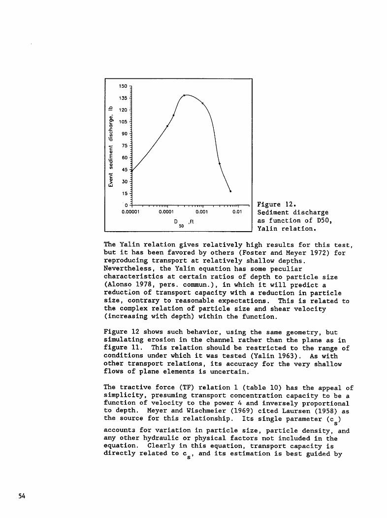
54

150 q

135 ^

^120 z

Q) i

0> 105 -^o -

.c !o 90 -.

TJ

^_, 75 -.c<u

E 60 :"•6

0)W

45 :*•<

cQ>> 30 i

UJ

15 :

n 1u n ' 'i 1 ' ' • • • •i• i i i i i 1111| i

0.00001 0.0001 0.001 0.01

D .ft50

Figure 12.Sediment dischargeas function of D50,Yalin relation.

The Yalin relation gives relatively high results for this test,but it has been favored by others (Foster and Meyer 1972) forreproducing transport at relatively shallow depths.Nevertheless, the Yalin equation has some peculiarcharacteristics at certain ratios of depth to particle size(Alonso 1978, pers. commun.), in which it will predict areduction of transport capacity with a reduction in particlesize, contrary to reasonable expectations. This is related tothe complex relation of particle size and shear velocity(increasing with depth) within the function.

Figure 12 shows such behavior, using the same geometry, butsimulating erosion in the channel rather than the plane as infigure 11. This relation should be restricted to the range ofconditions under which it was tested (Yalin 1963). As withother transport relations, its accuracy for the very shallowflows of plane elements is uncertain.

The tractive force (TF) relation 1 (table 10) has the appeal ofsimplicity, presuming transport concentration capacity to be afunction of velocity to the power 4 and inversely proportionalto depth. Meyer and Wischmeier (1969) cited Laursen (1958) asthe source for this relationship. Its single parameter (c )

accounts for variation in particle size, particle density, andany other hydraulic or physical factors not included in theequation. Clearly in this equation, transport capacity isdirectly related to c , and its estimation is best guided by

1000 -

5

discharge,o

o ij111iii

c = 200

c f = 100_^-»c0)

E'•o

<U to _

"c !

>Ld

0.1 1

llll| i

10 100

BC

0

Figure 13.Sediment discharge predicted A^ by the tractive forcerelation or law as function of parameter cs and _B, by theKilinc and Richardson relation as fuction of parameter c0.

comparing results of a range of values with a simple planeexample. Figure 13A shows the relation between sedimentproduction for a simple catchment and value of c . The

catchment consists of the single plane with a nonerodiblechannel from example 1. The particle diameter (D50) was takenas 0.00001 ft, c. - 0.0 and c = 0.003. By comparing the

results of figures 11 and 13A, one could choose cg to represent

a given particle size so that the results are similar to thosegiven by a more complex relation.

Similarly, parameter c in the relation from Kilinc and

Richardson (1973), attributed to Bagnold, directly determinesrelative transport capacity. Unlike the TF relation, however,factors of bed slope are also included as part of the shearterms. The critical shear limit is another difference between

this relation and the TF relation, so for flows with low bed

shear, erosion will be insensitive to values of c Like c

can be selected to represent a range of conditions andparticle sizes. Figure 13B illustrates the effect of c on

sediment production for the example 1 catchment and with othererosion parameters the same as for figure 13A.

55

56

Figure 13 also illustrates the three general behavior rangesthat may be exhibited in erosion and sediment transport on arunoff surface. These ranges are determined by the relativevalues of splash erosion, transport capacity, erosion rate, andsettling velocity. At very low values of transport capacityrelative to splash erosion rate, there is a minimum sedimentproduction from the plane determined by the ratio of productionto deposition. For this example, that value is about 25 lb ofsediment for the storm. This occurs although there is notransport capacity. The next range of behavior is the middlezone, where any increase in transport capacity is utilizedbecause of the continuing excess of splash erosion rate overtransport rate. Finally, as transport capacity increasesfurther relative to the other factors, splash rate becomes lesssignificant; and in the extreme, the rate of sediment off theend of the surface is governed by the rate of hydraulic erosion,which depends jointly on c and transport capacity.

Estimating Rainsplash Erosion Parameters

Parameters c_ and c, (equations [35] and [36]) are important in

controlling the rate at which rainfall energy produces loose,transportable particles from the soil surface. Often erosion islimited more by this rate of production than by the ability ofthe flowing surface water to transport the sediment. On theother hand, with flowing water and a rate of rainsplash erosionthat exceeds the rate of settling, sediment will move off thecatchment even with no transport capacity.

The value of c~ is clearly highest for loose, noncohesive,

unprotected soils. Its value has been related to cropping andslope factors by Foster et al. (1983), and their value forrelatively unprotected soil is related to the soil erodibilityfactor in the Universal Soil Loss Equation (Wischmeier and Smith1978). This value may be expressed in KINEROS units (feet andseconds) for estimation as follows:

c. = 422K n (<£-) [46]f usle ^f L J

The USLE handbook can be consulted for estimating values of thesoil erodibility factor (K , ) which are on the order of 0.1 to

J usle

0.5. Since English-metric conversions are not attempted forparameter c~, the metric and English input values should be

identical. The factor <£_. represents reductions due to mulch,

erosion pavement, vegetal cover, and other factors mitigatingsplash erosion. A more complete discussion of the estimation of<f>~ is found in Foster et al. (1983). The model user's judgment

will ultimately be required to estimate the amount of reductionappropriate for the conditions of simulation.

The parameter c, controls the effect of surface water depth on

raindrop detachment. After surface water forms, it reducessplash erosion by absorbing kinetic energy from the raindrops;and the extent of reduction varies directly with depth of thesurface water (Mutchler and Larson 1971, Schultz et al. 1985).KINEROS employs a conservative estimate for this damping,expressed in equation [36]. With depths expressed in feet, asused internally in KINEROS, and representing raindrop diameterby d^, using a value of 2/d for c, will reduce splash erosion

by roughly 50 percent for a water depth of one-third dropdiameter; this is in general agreement with publishedexperimental results. It represents a value of 203 for c, when

h

mean drop diameter is 3 mm. Since soil surfaces are neveruniform, both shallower and deeper water cover will be presentat any time.

Estimating the Hydraulic Erosion Coefficient

The hydraulic erosion coefficient (c ) represents the relativeg

rate of erosion by flowing water when the hydraulic conditionsfor the selected transport capacity relation indicate a largertransport capacity than the local concentration (equation [37]).This parameter is larger for loose, noncohesive soils than forcohesive soils that resist erosion. Foster and Smith (1984)estimated this parameter to be related to K _ and fractional

usle

clay content (f ) in the following manner:

c = 5.6 K _ <f> /am T471g usle *r ' T l^'J

with a = 188 -468f .+ 907f .2; f,< 0.22;•!• Ci Cl cl

or a = 130; f > fj.221 cl

This set of equations estimates c values (ft ) on the order ofS

0.001 to 0.02. Kugle is assumed to be in English units asreported by Wischmeier and Smith (1978). The factor <b

r

(dimensionless, 0-1.0) accounts for erosion resistance due tomulches or other management practices.

57

Describing theGeometry andCharacteristics

of a Pond

58

Partially "Paved" Catchments

A parameter PAVE is included in KINEROS to represent the part ofa "plane" element that is nonerodible because of pavement orother resistant cover. PAVE - 0 represents completely soilcovered surfaces, and PAVE -1.0 halts erosion completely as fora parking lot. This parameter can be used to account for desertpavement or rock mulch.

A pond is described for use in KINEROS by specifying a set ofcross sections that lie normal to the path of flow through thepond. Water is assumed to enter the pond at one end and toexit through an outlet, with a known relation between dischargeand depth of overfall, such as a weir or outlet orifice.

Description of the geometry of the pond requires preliminaryinterpretation of ordinary survey data. Sets of data pairs ofcross-sectional area below the waterline and bank-to-bank width

are required for sections in order, as described previously. Inaddition, these data are required at a fixed set of elevations.In other words, if one imagines the pond to be intersected by aset of level planes of fixed elevation, the data at each crosssection must be given for conditions as if the water level wereat each of those elevations.

The user is asked to describe the pond geometry by specifyingMEL (2-10) elevations, at which data will be supplied at several(NSEC) sections that are normal to the flow path. At eachsection and each elevation at that section, the user mustspecify the bank-to-bank width (TWP) and cross sectional area ofwater intersected by the section. Thus for section J andelevation I, one would describe AP(J,I) and TWP(J,I). Seefigure 7.

Other pond information required includes the distance along theflow path to each section (XSEC), the beginning water surfaceelevation (ELST), and the elevation of the lowest point on thepond bottom (ELVZ). The outflow rating is given by a table ofNOPQ pairs of elevation ELQ and corresponding discharge QSO.When sediment is to be routed through the pond, the user shouldsupply the number of particle size classes into which thesediment, with median particle size (D50), is to be subdivided.The particle sizes of the various classes are determined by thestandard deviation (SIGMAS) from the erosion data for the

element just above the pond. In addition, to account fordispersion, short circuiting, and diffusion, an effectivediffusivity coefficient (TDIFUS) may be specified for thedispersal of sediment during its travel through the pond.

2Values of TDIFUS on the order of 0.00001 to 0.0001 ft /s aresuggested.

Program Output Two output files are always created by the program. The typeand amount of detailed information in each are determined byswitches in the parameter file for each element. The basicoutput file is the hydrologic output. A second file containingdetailed computation results can be written for debugging ordetailed analysis.

The basic hydrologic output file always contains identifyinginformation, the names of input files read for the run, andhydrologic summary information. Optionally, it may containdetailed rainfall and runoff data. Sediment information is also

contained in this file if the sediment option is selected. Theamount of data output to this file is a function of eachelement's parameter NRP:

NRP = 0 Summary information only.

NRP = 1 Precipitation rate pattern written for this elementif a plane; if element is the last channel,precipitation data for last raingage read is output.

NRP = 2 Runoff hydrograph written for the element.

NRP = 3 Both precipitation rates and runoff hydrographwritten.

The auxiliary output file contains identifying information and asummary of calculations in the order of calculation. Thisoutput is determined by the value of the element's parameterNPRINT:

NPRINT = 1 No detailed output written for the element.

NPRINT = 2 Calculation results written. CAUTION: Depending onthe length of simulation, time step, and number ofelements for which this option is chosen, the outputcan be voluminous.

The most useful outputs will normally reside in the outputhydrograph file and in the rainfall and runoff plot files ifrequested. A sample output is shown in figure 14. The timeincrements for the output hydrograph and sediment concentrationwill be equal to the parameter DELT. The other columns areself-explanatory.

59

type exl.dat

INPUT POND FILE: DUMMY.PND

INPUT PARAMETER FILE: EX1.PAR

INPUT RAINFALL FILE: EX1.PRE

===== DESCRIPTIVE RUN TITLE —

KINEROS MANUAL EXAMPLE 1 - 4/13/89

VOL. BAL. SED. TOTAL

ELE #

1

TYPE

PLANE

ERROR % (LBS.)

0.127E-01 0.000

2 CHANNEL 0.381E+00 0.000

HYDROGRAPH FOR ELEMENT 2

CONTRIBUTING AREA= 20000.000 SQ. FEET OR 0.45913681 ACRES

TIME(MIN) Q(CFS) Q(IPH) CONC. QS(T/AC/HR)

0.00 0.00000 0.000000 0.00000000 0.OOOOE+00

0.50 0.00003 0.000054 0.00000000 0.OOOOE+00

1.00 0.00039 0.000838 0.00000000 0.OOOOE+00

1.50 0.00218 0.004708 0.00000000 0.OOOOE+00

2.00 0.00759 0.016404 0.00000000 0.OOOOE+00

2.50 0.02008 0.043369 0.00000000 0.OOOOE+00

3.00 0.04349 0.093936 0.00000000 0.OOOOE+00

3.50 0.07755 0.167512 0.00000000 0.OOOOE+00

4.00 0.11375 0.245693 0.00000000 0.OOOOE+00

4.50 0.14158 0.305812 0.00000000 0.OOOOE+00

5.00 0.15783 0.340913 0.00000000 0.OOOOE+00

* * * * *

* * * * *

59.00 0.00030 0.000640 0.00000000 0.OOOOE+00

59.50 0.00029 0.000620 0.00000000 0.OOOOE+00

60.00 0.00028 0.000601 0.00000000 0.OOOOE+00

TIME TO PEAK FLOW RATE = 9.0000 (MIN)PEAK FLOW RATE = 1.0777 (IPH)

Figure 14.Sample summary output file.

60

**** EVENT SUMMARY ****

GLOBAL VOLUME BALANCE

VALUES ARE IN UNITS OF LENGTH (VOL./BASIN AREA)

BASIN AREA - 20000.000 (FT**2)

TOTAL RAINFALL DEPTH = 0.200 (IN)

STORAGE REMAINING ON ALL PLANES = 0.00016 (IN)STORAGE REMAINING IN CHANNELS+CONDUITS - 0.00011 (IN)STORAGE REMAINING IN PONDS = 0.00000 (IN)TOTAL INFILTRATION FROM ALL PLANES = 0.00000 (IN)TOTAL INFILTRATION FROM ALL CHANNELS = 0.00000 (IN)TOTAL BASIN RUNOFF = 0.19894 (IN) 331.6 CU.FT

TOTAL OF STOR., INFIL. AND RUNOFF TERMS = 0.19922 (IN)

*** GLOBAL VOL. ERROR = 0.3925 PERCENT ***

Figure 14—Continued.Sample summary output file.

The detailed output is useful primarily for diagnostic purposes.An example is shown in figure 15. For those elements whenNPRINT = 2, the results of the finite difference computationswill be printed out for each time step. QL(IPH) is the net rateof lateral inflow, INFIL is the infiltration rate, SUP(I=1,NK)is the sediment supply rate and H2(I=1,NK) is the depth of flow(in feet) at each of the NK node points. CMX(I=1,NK) is theequilibrium sediment transport concentration at each node, andCT(I=1,NK) is the sediment concentration. DELH(I=1,NK)represents the amount of erosion (-) or deposition (+) at eachnode (in feet).

INFLOW, OUTFLOW, and STOR are volume balance terms in cubic feetfor the entire plane. INFLOW is the sum of the rainfall plusinflow from a contributing plane (RO FROM UPSTREAM) since time(t) =0. OUTFLOW is the sum of infiltration (INFIL) at eachnode plus the discharge from the lower boundary of the plane (ROOUT) . STOR is the amount of water stored on the plane at time(t). A positive ERROR indicates loss of water and negative anapparent gain. Although errors are usually less than 1 percent,they may be somewhat larger when an upper plane contributesrunoff to a lower plane where ponding has not yet occurred.These errors are due to kinematic shocks occurring under thesecircumstances, and the numerical methods used in KINEROS do notaccount for them explicitly. Errors greater than 1 percent mayalso occur when only five nodes are used for a channel with noupstream inflow.

61

type exl.aux

INPUT POND FILE: DUMMY.PNDINPUT PARAMETER FILE: EX1.PARINPUT RAINFALL FILE: EX1.PRE

— DESCRIPTIVE RUN TITLE


*** PLANE NO 1 DIAGNOSTIC INFORMATION ***

THE RAIN GAGE FOR PLANE 1 IS GAGE NO. 1

PPCT. WEIGHT IS 1.00 INTERCEPTION IS 0.01 (IN)

GEOM. PARAMETERS ARE L= 100.0 W=

ROUGHNESS COEF. IS MANNINGS N-0.013

IMPERVIOUS PLANE

200.0 S- 0.0500

INFLOW*

**** WATER BALANCE AT END OF PLANE ****

<INFLOW BASED ON (PPT*GAGE WT) - INTER. + RUNON>0.333E+03 OUTFLOW- 0.333E+03 STOR.- 0.268E+00 ERROR* 0.127E-01 %

** CHANNEL NO 2 DIAGNOSTIC INFORMATION **

T( 2)= 0.3000E+02 Q( 2)A2(K=1,NK)= 0.0000 0.00040.0004 0.0004 0.0004 0

UPPER INFLOW- 0.000E+00

CHAN. OUTFLOW- 0.376E-03

*

T( 60)= 0.1770E+04 Q( 60)A2(K=1,NK)= 0.0000 0.00200.0083 0.0091 0.0098 0.

UPPER INFLOW- 0.000E+00

CHAN. OUTFLOW- 0.328E+03

0.2508E-04 QL( 2)= 0.2543E-040.0004 0.0004 0.0004 0.0004 0.0004

0004 0.0004 0.0004 0.0004

0.763E-01 INFIL. OUTFLOW-

ERROR-

LAT, INFLOW*

STORAGE- 0.736E-01

*

*

= 0.8666E-02 QL( 60)= 0.2539E-040.0031 0.0041 0.0051 0.0059 0.0067

0106 0.0113 0.0120 0.0128

LAT. INFLOW- 0.331E+03 INFIL. OUTFLOW-

STORAGE- 0.146E+01 ERROR=

T(121)= 0.3600E+04 Q(121)= 0.2783E-03 QL(121)= 0.8230E-06A2(K=1,NK)= 0.0000 0.0002 0.0004 0.0005 0.0006 0.0008 0.00090.0011 0.0012 0.0012 0.0013 0.0014 0.0015 0.0016

UPPER INFLOW- 0.000E+00 LAT. INFLOW- 0.333E+03 INFIL. OUTFLOW-

CHAN. OUTFLOW- 0.332E+03 STORAGE- 0.185E+00 ERROR=

GEOM. PARAMETERS ARE L= 200.0 S= 0.0300

TRAP. X-S LEFT SLOPE- 1.000 RIGHT SLOPE- 1.000 BOTT. WID.=

ROUGHNESS COEF. IS MANNINGS N= 0.013

IMPERVIOUS CHANNEL

CONTRIB. CHANNEL NUMBERS: NCI- 0 NC2- 0

CONTRIB. PLANE NUMBERS: LEFT- 1 RIGHT- 0 UPPER= 0

*** WATER BALANCE AT END OF CHANNEL ***

<INFLOW BASED ON RUNIN + LATERAL INFLOW>

INFLOW- 0.333E+03 OUTFLOW- 0.332E+03 STOR.- 0.185E+00 ERROR- 0.381E+00 %

0.0004

0.000E+00

0.308E+01 %

*

0.0075

0.000E+00

0.389E+00 %

0.0010

0.000E+00

0.381E+00 %

2.00

Figure 15.Sample auxiliary output file.

62

Example 1

EXAMPLES USING HYPOTHETICAL WATERSHEDS

Three examples using hypothetical watersheds have been developedto demonstrate features of KINEROS and the preparation of inputdata files.

We will describe procedures to create input files for thehypothetical watershed shown in figure 16. In this example, theplane, element 1, contributes lateral inflow to a trapezoidalchannel, element 2. We name the input parameter file EX1.PARand start by copying the template file TEMP.PAR to EX1.PAR. Weuse an editor to fill in input values below the parameter names.

Figure 16.Hypothetical watershed.

A printout of the completed file EX1.PAR is shown in figure 17.There are eight parameters under the heading "SYSTEM." NELErefers to the number of watershed elements (planes, channels,and ponds), so we enter 2. NRES refers to the resistance law tobe used. We use NRES-1, which is Manning's law. NPART isneeded only for pond elements. CLEN is a characteristic lengththat is used within the program to choose the length of Axincrements in the finite difference solutions. It should

normally be set equal to the sum of the lengths of the longestcascade of planes in the system or the longest single channelwhichever is greater. For this example, the channel lengthcontrols and CLEN - 200 ft.

TFIN is the desired maximum duration for runoff computations.It is based on the length of the rainfall event and thewatershed response time. Assume that for this example we wishthe program to stop after it has computed a runoff hydrographwith a duration of 60 minutes from the beginning of the rain.Therefore TFIN - 60.

63

64

type exl.par

KINEROS Parameter Input File

**********************************

*********** SYSTEM ********

**********************************

* NELE NRES NPART CLEN TFIN DELT THETA

2 10 200. 60. 0.5 0.6

#

***********************************

********* OPTIONS ***********

***********************************

NTIME NUNITS NEROS

2 10

#

***********************************************

**** COMPUTATION ORDER ****

***********************************************

There must be NELE elements in the list. NLOG

must be sequential. ELEMENT NUM. need not be.#

COMP. ORDER ELEMENT

(NLOG) NUM. (J)

TEMP

-1.

#

***********************************************

****** ELEMENT-WISE INFO ***

***********************************************


NU

0

XL

100.0

FMIN

0.0

LAW

0

NU

0

NR

0

W

200.0

G

0.0

CF

0.0

NR

0

NL

0

S

05

POR

0.0

CG

0.0

NL

1

NCI

0

ZR

0.0

SI

0.0

NC2

0

ZL

0.0

SMAX

0.0

CH CO-CS

0.0 0.0

NCASE NPRINT

0 1

BW

0.0

DIAM

0.0

NPNT

0

Rl

013

NRP

0

R2

0.0

ROC

0.0

RECS DINTR

0.0 0.01

D50

0.0

RHOS

0.0

PAVE SIGMAS

0.0 0.0

NCI NC2 NCASE NPRINT NPNT NRP

0 0 12 0 0

XL W S ZR ZL BW DIAM Rl R2

200. 0 .0 .03 1. 1. 2. 0.0 0 013 0.0

FMIN

0.0

G

0.0

POR

0.0

SI SMAX

0.0 0.0

ROC RECS DINTR

0.0 0.0 0.0

LAW CF CG CH CO-CS D50 RHOS PAVE SIGMAS

0 0.0 0.0 0.0 0.0 0.0 0.0 0.0 0.0

Figure 17.Parameter file for example 1.

DELT is the time increment for computations and printout of thehydrograph. For this example we use DELT = 0.5 min.

THETA is the weighting factor in the implicit numericalsolution. It must be between 0.5 and 1. As THETA approaches1.0, more numerical dispersion is introduced into the solution.In this example there will be no kinematic shocks, so we selectTHETA =0.6. (If kinematic shocks are likely to occur, THETA =0.8 is recommended.)

TEMP is the temperature in degrees Fahrenheit (for English unitinput). It is used to calculate the kinematic viscosity ofwater. If TEMP is set to -1, a default temperature of 65°F isused. We will use the default value.

There are three parameters under the heading "OPTIONS." NTIMErefers to the use of seconds or minutes as units of time for

input data and time variables DELT and TFIN. Since we use NTIME= 2, input will be in minutes. We use NUNITS = 1, so all inputis in English units. We do not use the erosion option in thisexample, so NEROS = 0.

The next heading is "COMPUTATION ORDER" with column headingsNLOG and ELEMENT NUM.(J). These integer variables control theorder of computations. Entries under NLOG are consecutiveintegers starting with 1 and ending with NELE. Under ELEMENTNUM.(J), we enter 1 and 2. This means that the computationswill be completed first for element 1 (the plane) and then forelement 2 (the channel). The entries under ELEMENT NUM.(J) neednot be consecutive integers; however, the outflow hydrographs ofall elements contributing upstream inflow or lateral inflow tothe element J must be computed before the computations canproceed for element J.

Under the heading "ELEMENT-WISE INFO," we enter the geometricdescription of each plane and channel and the infiltration anderosion parameters if required. The elements can be entered inany order, but it is most convenient to enter them in order,beginning with element 1.

The variable J refers to the element number, so we enter 1 for

the plane and 2 for the channel. There are no planescontributing to the upper boundary of plane 1, so NU = 0. NRthrough NCASE are valid only for channels, so we enter a zero ineach column. We do not wish a diagnostic printout, so NPRINT =1. This is not a pond, so NPNT - 0. We do not wish to printout rainfall or runoff data for this element, so NRP = 0. Thelength (100 ft), width (200), and slope (0.05) are entered underXL, W, and S, respectively. ZR through DIAM apply only forchannels, so zeros are entered. Because we have selected NRES =

65

66

1, Rl refers to the Manning's n value. If we assume that plane1 has an asphalt surface, an appropriate value for Rl is 0.013.With NRES - 1, R2 is inoperative, so we enter a zero. The planeis impervious, so FMIN =0.0. With the options chosen, zeroscan be entered for all other parameters except the interceptionDINTR, which we assume is 0.01 in.

For the channel (element 2), NU = 0 since no plane contributesto the upper boundary. Plane 1 contributes lateral inflow tothe left side of the channel, so NL = 1. NR = 0 because thereis no contribution to the right side. Similarly NCI and NC2 arezero because no channels contribute to the upper boundary ofchannel 2. The channel is trapezoidal, so NCASE - 1. We selectthe detailed printout option, so NPRINT - 2. As discussedbefore, NPNT and NRP are both zero. We enter the channel length(200) under XL and a zero under W. W= 0 indicates a channel.The channel slope (S) = 0.03. For a trapezoidal channel with a2-ft bottom width and 1:1 side slopes, ZR = 1., ZL = 1., and BW= 2. For Manning's n we again select Rl - 0.013. All otherparameters can be set to zero.

The parameter and geometry file is now complete, so we createthe precipitation input file. We begin by copying the templatefile TEMP.PRE to the file EX1.PRE. The completed precipitationinput file is shown in figure 18. Under the heading "GageNetwork Data," we have two parameters. NGAGES is the number ofraingages. In this example NGAGES - 1. MAXND refers to themaximum number of time-depth pairs in the rainfall data. Let usassume that the cumulative rainfall and the intensity histogramare as shown in figure 19. We will need five time-depth pairsto represent the rainfall pattern since rainfall must be definedpast TFIN. Therefore MAXND = 5. The next data, ELE. NUM. (J),RAINGAGE, and WEIGHT, provide a means of weighting the rainfallat a given gage by a multiplier, WEIGHT, to get the correctrainfall for ELEMENT(J). We have only one gage, which we willcall gage 1, and its weight will be 1 for elements 1 and 2.Under the heading "Rainfall Data," we enter the parameter ND,which is the number of time depth pairs for the specific gage,starting with gage 1. In this case ND - 5. The time (TIME) andaccumulated rainfall depth pairs (ACCUM. DEPTH) are enterednext.

Part of the output hydrograph file is shown in figure 14 andpart of the detailed or auxiliary output file is shown in figure15. &

The standard output file (fig. 14) shows the names of the inputparameter file and rainfall file, the volume balance errors andtotal erosion for each element, the contributing area, theoutflow hydrograph and sedigraph, peak flow rate statistics, andtotals of input and output.

type exl.pre


****************************

Gage Network Data****************************

NUM. OF RAINGAGES

(NGAGES)MAX. NUM. OF TIME-DEPTH DATA PAIRS FOR ALL GAGES

(MAXND)

1 5

p


ELE. NUM. (J)

1

2

RAINGAGE

1

1

WEIGHT

1.0

1.0

#

*****************************

Rainfall Data*****************************


#

* ALPHA-NUMERIC GAGE ID: EXAMPLE 1 - GAGE 1 = GAGE 1.

rr


1 5

#

There must be ND pairs of time-depth (T D) data: NOTE: The last timemust be greater than TFIN (the total computational time)

TIME ACCUM. DEPTH

0.0 0.00

5.0 0.04

10.0 0.13

20.0 0.21

65.0 0.21*

Figure 18.Precipitation input file for example 1.

c

Q.Q)

o

1.0

0.5-

\fRainfall intensity

10 20

Time (min)

30

Accumulated depth

i

40

i

50 60

-1

70

Figure 19.Rainfall intensitypattern forexample 1.

67

The auxiliary file, figure 15, includes a summary of parametergeometry, and water balance information for each element andallows detailed printouts to be made for any element whereNPRINT =2. For example 1, NPRINT - 2 for the channel, element2, and results of computations for each time step are printedout. T is the time in seconds, Q is the discharge at thedownstream boundary of the element in cubic feet per second, QLis the lateral inflow in cubic feet per second per foot and'A2(K-1,NK) is the cross sectional area in square feet at eachnode for that time. In this case, there were 15 nodes (NK =15). The auxiliary file is useful primarily for programdebugging and for checking input parameter files. It is alwayswise to scan the water balance information in this file and todetermine the reason for any error greater than 2-3 percent.

Example 2 In this example, we demonstrate the following features:Infiltration, erosion, branching channels, circular conduit, andmultiple raingages. The seven-element watershed geometry isshown in figure 20. Elements 1 and 2 are identical to those inexample 1. Any changes in input data from example 1 for theseelements are discussed. We assume that erosion occurs only oninfiltrating planes and trapezoidal channels. The circularconduit is nonerodible, although deposition and subsequenterosion of that deposited material are possible. The inputparameter file EX2.PAR is shown in figure 21. NELE is now 7NRES is 2 signifying that the resistance option 2, Laminar-Manning, will be used. CLEN is 300 ft, the sum of the lengthsof planes 4 and 7. DELT has been increased from 0.5 to 1.0min reflecting the increase in CLEN. TFIN has been increasedto 90 minutes to reflect the slower response time of thiswatershed compared with that in example 1. THETA has beenincreased to 0.8 because we have cascading planes. Under"OPTIONS" note that NEROS - 2, signifying that we are electingthe erosion option. The computational order is 1, 2, 3, 7, 4,5, 6. Note that the following orders are also feasible' 3* 7*4, 5, 1, 2, 6 and 7, 4, 3, 5, 1, 2, 6. ' '

Input for element 1 is identical to that for example 1 exceptthat we have entered 80 under R2 for the Laminar "k" valueUnder LAW we enter 1, the code for the tractive force erosionlaw. We have entered values for CG (0.011), CS (0 001) D50(0.0005), RHOS (2.65), POR (0.40), and PAVE (1.0) as requiredfor the tractive force law. Note, however, that PAVE = 1 haltserosion detachment. CF = 0 also halts rainsplash erosion.

68

aingage I

DIAM=2ft

Figure 20.Elements used in example 2.

For channel element 2 the input is identical to that in example1 except that LAW = 2, which specifies the unit stream powerrelation with CG = 0.011, D50 (0.0005), RHOS (2.65), POR (0.40),and PAVE (1.0), which prevents erosion. We have also suppressedthe detailed printout by setting NPRINT = 1. Elements 1 and 2correspond to a paved parking lot drained by a paved channel.

For plane element 3 we have chosen values of Rl and R2 torepresent a sparsely vegetated rangeland watershed (see table4). SMAX = 0.83, FMIN = 0.068 in/h, POR = 0.40, and G = 10.4 inrepresent a sandy clay loam soil (see table 2). Note that wehave approximated Ks under imbibition by dividing the tabulated

K by 2.s J

The effect of rock is estimated by multiplying K by

(1. - ROC). The initial saturation (SI) is 0.25. The soil has20 percent rock by volume. RECS =0.2 in, so the water depthduring recession must be greater than this depth for the entirewetted area to contribute to infiltration. The interception(DINTR) = 0.03 in.

69

70

type ex2.par

#

**********************************

*********** SYSTEM ******************************************

* NELE NRES NPART CLEN TFIN7 2 0 300. 90.

#

***********************************

********* OPTIONS **********************************************

NTIME NUNITS NEROS

2 12#

***********************************************


There must be NELE elements in the list. NLOGmust be sequential. ELEMENT NUM. need not be.

#

COMP. ORDER ELEMENT

(NLOG) NUM. (J)


DELT

1.0

THETA

0.8

TEMP

-1.

#

***********************************************



*

J NU NR NL NCI NC2 NCASE NPRINT NPNT NRP1000000100

XL W S ZR ZL BW DIAM Rl R2100.0 200.0 0.05 0.0 0.0 0.0 0.0 0.013 80.0

FMIN

0.0

LAW

1

NU

0

G

0.0

CF

0.0

NR

0

POR

0.4

CG

0.011

NL

1

SI SMAX

0.0 0.0ROC RECS DINTR

0.0 0.0 0.01

CH CO-CS D50 RHOS PAVE SIGMAS

0.0 0.001 0.0005 2.65 1.0 0.0

NCI NC2 NCASE NPRINT0 0 11

NPNT NRP

0 0

Figure 21.Input parameter file for example 2.

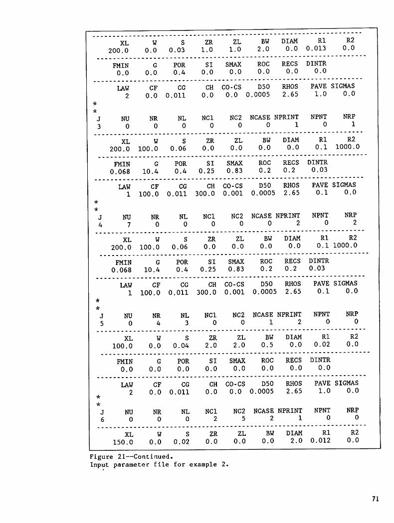
XL

200.0

W

0.0

S

0.03

ZR

1.0

ZL

1.0

BW

2.0

DIAM

0.0

Rl

0.013

R2

0.0

FMIN

0.0

G

0.0

POR

0.4

SI

0.0

SMAX

0.0

ROC

0.0

RECS

0.0

DINTR

0.0

*

*

J

3

LAW

2

NU

0

CF

0.0

NR

0

CG

0.011

NL

0

CH

0.0

NCI

0

CO-CS

0.0 C

NC2

0

D50 RHOS

1.0005 2.65

NCASE NPRINT

0 1

PAVE SIGMAS

1.0 0.0

NPNT NRP

0 1

XL

200.0

w

100.0

S

0.06

ZR

0.0

ZL

0.0

BW

0.0

DIAM

0.0

Rl

0.1

R2

1000.0

FMIN

0.068

G

10.4

POR

0.4

SI

0.25

SMAX

0.83

ROC

0.2

RECS

0.2

DINTR

0.03

*

*

J

4

LAW

1

NU

7

CF

100.0

NR

0

CG

0.011

NL

0

CH

300.0

NCI

0

CO-CS

0.001

NC2

0

D50

0.0005

NCASE 1

0

RHOS

2.65

NPRINT

2

PAVE

0.1

NPNT

0

SIGMAS

0.0

NRP

2

XL

200.0

W

100.0

S

0.06

ZR

0.0

ZL

0.0

BW

0.0

DIAM

0.0

Rl

0.1

R2

1000.0

FMIN

0.068

G

10.4

POR

0.4

SI

0.25

SMAX

0.83

ROC

0.2

RECS

0.2

DINTR

0.03

*

*

J

5

LAW

1

NU

0

CF

100.0

NR

4

CG

0.011

NL

3

CH

300.0

NCI

0

CO-CS

0.001

NC2

0

D50

0.0005

NCASE

1

RHOS

2.65

NPRINT

2

PAVE

0.1

NPNT

0

SIGMAS

0.0

NRP

0

XL

100.0

W

0.0

S

0.04

ZR

2.0

ZL

2.0

BW

0.5

DIAM

0.0

Rl

0.02

R2

0.0

FMIN

0.0

G

0.0

POR

0.0

SI

0.0

SMAX

0.0

ROC

0.0

RECS

0.0

DINTR

0.0

*

*

J

6

LAW

2

NU

0

CF

0.0

NR

0

CG

0.011

NL

0

CH

0.0

NCI

2

CO-CS

0.0

NC2

5

D50

0.0005

NCASE

2

RHOS

2.65

NPRINT

1

PAVE

1.0

NPNT

0

SIGMAS

0.0

NRP

0

XL

150.0

W

0.0

S

0.02

ZR

0.0

ZL

0.0

BW

0.0

DIAM

2.0

Rl

0.012

R2

0.0

Figure 21—Continued.Input parameter file for example 2.

71

72

FMIN

0.0

G

0.0

POR

0.0

SI

0.0

SMAX

0.0

ROC

0.0

RECS

0.0

DINTR

0.0

*

*

J

7

LAW

2

NU

0

CF

0.0

NR

0

CG

0.011

NL

0

CH

0.0

NCI

0

CO-CS

0.0

NC2

0

D50

0.0005

NCASE

0

RHOS

2.65

NPRINT

1

PAVE

1.0

NPNT

0

SIGMAS

0.0

NRP

3

XL

100.0

W

200.0

S

0.01

ZR

0.0

ZL

0.0

BW

0.0

DIAM

0.0

Rl

0.012

R2

100.0

FMIN

0.0

G

0.0

POR

0.0

SI

0.0

SMAX

0.0

ROC

0.0

RECS

0.0

DINTR

0.0

*

LAW

1

CF

0.0

CG

0.011

CH

0.0

CO-CS

0.0

D50

0.0005

RHOS

2.65

PAVE

1.0

SIGMAS

0.0

Figure 21—Continued.Input parameter file for example 2.

Plane 3 will be subject to erosion using the tractive forceerosion law. The raindrop splash erosion parameters (CF and CH)are 100 and 300, respectively. The hydraulic erosioncoefficient (CG) = 0.011 and the parameter (CS) - 0.001. Themedian diameter (D50) - 0.0005 ft. The particle specificgravity (RHOS) = 2.65, and the surface has 10 percent rock cover(PAVE =0.10). NRP - 1, so the rainfall rates will be printedfor this element. The remaining data are self-explanatory.

Note that plane 7 is impervious and contributes runoff to plane4, which is pervious and erodible. Channels 5 and 6 areimpervious and nonerodible. Hydrograph data and the detailedfinite difference solution will be printed for element 4 (NRP =2 and NPRINT = 2), and both rainfall and runoff rates will beprinted for element 7 (NRP =3). Note that values for D50 andRHOS have been included for all elements.

The rainfall data file EX2.PRE is shown in figure 22. Becausethere are two raingages, NGAGES = 2. There are six time-depthpairs for raingage 2, so MAXND - 6. We will assume that planes1 and 3 are nearest to gage 1 and planes 4 and 7 are nearest togage 2. We must assign values of RAINGAGE and WEIGHT to thechannel elements, but the actual values put in are irrelevantbecause they are not used. The WEIGHT values would normally beestimated from an isohyetal map of the storm. We will assumethat the storm depth at plane 4 was 0.95 in, so WEIGHT =0.95/0.90 =1.06. If the depth at plane 3 was 0.98 in, thenWEIGHT = 0.98/1.00 =0.98. Note that rain started 1 minutelater at gage 2 than at gage 1, so it is possible to simulatestorm movement.

type ex2.pre

KINEROS Rainfall Input Data#

****************************


#

NUM. OF RAINGAGES MAX. NUM. OF TIME-DEPTH DATA PAIRS FOR ALL GAGES

(NGAGES) (MAXND)

2 6

There must be NELE pairs of (GAGE WEIGHT) data*

ELE. NUM. (J) RAINGAGE

1

WEIGHT

1 1.0

2 1 1.0

3 1 0.98

4 2 1..06

5 2 1.0

6 2 1.0

7 2 1.0

*****************************

Rainfall Data*****************************


* ALPHA-NUMERIC GAGE ID: EXAMPLE 2 - GAGE 1 = GAGE 1; 2=2.#



TIME ACCUM. DEPTH

0.0 0.0

5.0 0.2

10.0 0.6

20.0 1.0

150.0 1.0

* ALPHA-NUMERIC GAGE ID: EXAMPLE 2 - GAGE 1 = GAGE 1; 2 = 2



4-

TIME ACCUM. DEPTH

0.0 0.00

1.0 0.00

6.0 0.20

11.0 0.58

21.0 0.90

150.0 0.90

Figure 22.Rainfall input data for example 2

73

74

Parts of the summary output file are shown in figure 23. Theelement number, type of element (plane or channel), volumebalance error, and sediment transport output are shown for eachelement in computational order. The hydrograph for plane 7 isshown because NRP - 3 for that element. The hydrograph,sediment concentration, and sediment transport are always shownfor the last element (in this example, channel 6). Finally thepeak discharge rate, time to peak, total rainfall, waterremaining in storage, total infiltration, total runoff andglobal volume balance error are given. The total rainfall willbe the total for the storm given in the rainfall input fileweighted by the area of each plane element. The total runoffwill be the integral of the hydrograph up to time TFIN.

Part of the auxiliary output file is shown in figure 24.Diagnostic information is provided for each element incomputational order. The rainfall hyetograph is printed out forplane 3 because NRP = 1, and for plane 7 because NRP = 3. Forplane 4 (NPRINT = 2), the detailed printout shows the finite-difference solutions for the net sediment supply rate (SUP(I)),depth (H2(I)), sediment transport capacity (CMX(I)), and localsediment concentration (CT(I)), along with the lateral inflowrate (QL), infiltration rate (INFIL), and the accumulated changein bed elevation (DELH(I)) at four selected times.

At TIME =0.0, rainfall has not yet started so all variables areset equal to zero. At TIME = 180 s, ponding has occurred at allnodes and inflow from impervious plane 7 is evidenced byincreased depths at nodes 1 and 2. The flow depths at all nodesexcept node 1 are too small to provide sediment transportcapacity (CMX); however, rain splash provides some erosion sothe sediment concentrations (CT) are greater than zero except atnode 1 where clear water is advected from nonerodible plane 7.The message NO POSITIVE ROOT AT J = 2 indicates a numericalproblem associated with kinematic shock. This shock initiatesperturbations in the depth that cause perturbations in thesediment transport capacity. This variation in CMX is reflectedin the sediment supply term SUP alternating between erosion (+)and deposition (-).

At TIME = 480 s, the rainfall is at the maximum intensity anderosion is occurring at all nodes except node 8. The greatestamount of erosion (DELH) has occurred at node 1. The greatestdepth and transport capacity is at node 2. The concentrationprofile reflects the upstream boundary condition (CT=0) and hasa maximum at node 4.

At TIME = 1380 s, the rainfall rate has been zero for 60 s.Lateral inflow is equal to the negative of the infiltrationrate. Erosion is occurring at the upper 5 nodes and depositionis taking place at the lower 5 nodes. All nodes showaccumulated erosion, but perturbations introduced while theshock traversed plane 4 persist.

type ex2.dat

INPUT POND FILE: DUMMY.PNDINPUT PARAMETER FILE: EX2.PARINPUT RAINFALL FILE: EX2.PRE

— DESCRIPTIVE RUN TITLE


ELE #

1

2

3

7

TYPE

PLANE

CHANNEL

PLANE

PLANE

VOL. BAL.

ERROR %

0.990E+00

0.641E+00

-0.600E-01

-0.395E+00

SED. TOTAL

(LBS.)

0.000

0.000

50.237

0.000

CONTRIBUTING AREA*

HYDROGRAPH FOR ELEMENT 720000.000 SQ. FEET OR 0.45913681 ACRES


0.00 0.00000 0.000000 0.00000000 0.OOOOE+00

1.00 0.00000 0.000000 0.00000000 0.OOOOE+00

2.00 0.01687 0.036449 0.00000000 0.OOOOE+00

3.00 0.13499 0.291589 0.00000000 0.OOOOE+00

4.00 0.45561 0.984113 0.00000000 0.OOOOE+00

5.00 0.91709 1.980918 0.00000000 0.OOOOE+00

* * * * *

* * * *

86.00 0.00305 0.006582 0.00000000 0.OOOOE+00

87.00 0.00298 0.006432 0.00000000 0.OOOOE+00

88.00 0.00291 0.006288 0.00000000 0.OOOOE+00

89.00 0.00285 0.006148 0.00000000 0.OOOOE+00

90.00 0.00278 0.006014 0.00000000 0.OOOOE+00

TIME TO PEAK FLOW RATE - 10.000 (MIN)

PEAK FLOW RATE 4.5603 (IPH)

ELE # TYPE

5 CHANNEL

6 C.COND.

VOL. BAL.

ERROR %

0.208E+01

-0.106E-01

Figure 23.Parts of summary output file for example 2

SED. TOTAL

(LBS.)

345.061

345.060

75

76

CONTRIBUTING AREA=

TIME(MIN)

HYDROGRAPH FOR ELEMENT

80000.000 SQ. FEET OR

Q(CFS) Q(IPH)

1.8365473 ACRES

CONC. QS(T/AC/HR)

0.00 0.00000 0.000000 0.00000000 0.OOOOE+001.00 0.00040 0.000216 0.00000000 0.OOOOE+002.00 0.07016 0.037888 0.00000000 0.OOOOE+003.00 0.43391 0.234311 0.00000000 0.OOOOE+004.00 0.85646 0.462490 0.00000000 0.OOOOE+005.00 1.02774 0.554980 0.00000000 0.1181E-09* * * * *

* * * * *

86.00 0.00272 0.001467 0.00000000 0.4730E-1087.00 0.00261 0.001408 0.00000000 0.3765E-10

88.00 0.00250 0.001351 0.00000000 0.2889E-1089.00 0.00240 0.001298 0.00000000 0.2125E-10

90.00 0.00231 0.001248 0.00000000 0.1530E-10

TIME TO PEAK FLOW RATE = 13.000 (MIN)

-

PEAK FLOW RATE 2.9247 (IPH)




BASIN AREA 80000.000 (FT**2)

TOTAL RAINFALL DEPTH = 0.941 (IN)

STORAGE REMAINING ON ALL PLANES

STORAGE REMAINING IN CHANNELS+CONDUITS

STORAGE REMAINING IN PONDS

TOTAL INFILTRATION FROM ALL PLANES

TOTAL INFILTRATION FROM ALL CHANNELS

TOTAL BASIN RUNOFF

TOTAL OF STOR., INFIL. AND RUNOFF TERMS

*** GLOBAL VOL. ERROR

Figure 23--Continued.Parts of summary output file for example 2

0.01245 (IN)0.00016 (IN)0.00000 (IN)0.19913 (IN)0.00000 (IN)0.71686 (IN)

0.92859 (IN)

1.3185 PERCENT ***

4779.1 CU.FT,

type ex2.aux

INPUT POND FILE: DUMMY.PND



=== DESCRIPTIVE RUN TITLE —





GEOM. PARAMETERS ARE L= 100.0 W= 200.0 S= 0.0500

ROUGHNESS COEF. ARE MANNINGS N=0.013 LAMINAR K- 80.0

IMPERVIOUS PLANE

EROSION PARAMETERS ARE ---

LAW- 1 CF-0.000E+00 CG-0.110E-01 CH- 200. CO-0.100E-02

CS-0.100E-02 D50-0.500E-03 RHOS= 2.65 POR- 0.40 PAVE.FAC-

ACCUMUL. SURFACE DEPOSIT. OR EROSION (NEG.) AT EACH NODE (FT.)O.OOOOOE+00 O.OOOOOE+00 O.OOOOOE+00 O.OOOOOE+00 O.OOOOOE+00

1.000


<INFLOW BASED ON (PPT*GAGE WT) - INTER. + RUNON>INFLOW- 0.165E+04 OUTFLOW- 0.162E+04 STOR.- 0.905E+01 ERROR= 0.990E+00 %

** CHANNEL NO 2 DIAGNOSTIC INFORMATION **

GEOM. PARAMETERS ARE L= 200.0 S= 0.0300

TRAP. X-S LEFT SLOPE- 1.000 RIGHT SLOPE- 1.000 BOTT. WID.= 2.00

ROUGHNESS COEF. IS MANNINGS N= 0.013

IMPERVIOUS CHANNEL

CONTRIB. CHANNEL NUMBERS: NCI- 0 NC2= 0

CONTRIB. PLANE NUMBERS: LEFT= 1 RIGHT= 0 UPPER= 0


LAW- 2 CG-0.110E-01 CO-0.000E+O0 CS-0.000E+0O

D50-0.500E-03 RHOS- 2.65 SURF.POR.= 0.40 PAVE. FAC- 1.000

ACCUMUL. CHAN. BOTTOM DEPOSIT. OR EROSION (NEG.)AT EACH NODE (SQ.FT.)0.000000 0.000000 0.000000 0.000000 0.000000 0.000000 0.000000 0.000000

0.000000 0.000000



0.162E+04 OUTFLOW- 0.161E+04 STOR.= 0.475E+00 ERROR= 0.641E+00 %INFLOW=


RAINFALL HYETOGRAPH FOR PLANE NO

(AFTER INTERCEPTION REMOVED)

Figure 24.Auxiliary output file for example 2.

77

TIME (MIN) INTENSITY(IN/HR)0.0 1.99

5.0 4.70

10.0 2.35

20.0 0.00

150.0 0.00

150.1 0.00



GEOM. PARAMETERS ARE L= 200.0 W= 100.0 S- 0.0600

ROUGHNESS COEF. ARE MANNINGS N-0.100 LAMINAR K= 1000.0

INFILT. PARAMETERS ARE FMIN- 0.06800 G= 10.400 SI- 0.25

POR- 0.400 SMAX- 0.83 ROC- 0.20 RECS- 0.200


LAW- 1 CF- 100. CG-0.110E-01 CH- 300. CO-0.100E-02

CS-0.100E-02 D50-0.500E-03 RHOS- 2.65 POR- 0.40 PAVE.FAC- 0.100ACCUMUL. SURFACE DEPOSIT. OR EROSION (NEG.) AT EACH NODE (FT.)

-0.44567E-05 -0.11217E-03 -0.33075E-04 -0.83216E-05 -0.41094E-04 -0.21475E-040.50459E-04 -0.31442E-04 -0.59458E-04 -0.38744E-04


<INFLOW BASED ON (PPT*GAGE WT) - INTER. + RUNON>INFLOW- 0.158E+04 OUTFLOW- 0.157E+04 STOR.- 0.147E+02 ERROR—0.600E-01 %

*** PLANE NO. 7 DIAGNOSTIC INFORMATION ***

RAINFALL HYETOGRAPH FOR PLANE NO. 7

(AFTER INTERCEPTION REMOVED)TIME (MIN) INTENSITY(IN/HR)

0.0 0.00

1.0 2.40

6.0 4.56

11.0 1.92

21.0 0.00

150.0 0.00



GEOM. PARAMETERS ARE L= 100.0 W= 200.0 S- 0.0100

ROUGHNESS COEF. ARE MANNINGS N-0.012 LAMINAR K- 100.0

IMPERVIOUS PLANE


LAW- 1 CF-O.000E+00 CG-0.110E-01 CH= 200. CO-0.000E+00CS-O.000E+0O D50-0.500E-03 RHOS- 2.65 POR- 0.40 PAVE.FAC- 1.000

ACCUMUL. SURFACE DEPOSIT. OR EROSION (NEG.) AT EACH NODE (FT.)).00000E+00 O.OOOOOE+00 O.OOOOOE+00 O.OOOOOE+00 O.OOOOOE+00


<INFLOW BASED ON (PPT*GAGE WT) - INTER. + RUNON>INFLOW- 0.150E+04 OUTFLOW= 0.148E+04 STOR.- 0.227E+02 ERROR--0.395E+00 S

Figure 24--Continued.Auxiliary output file for example 2

78


THE RAIN GAGE FOR PLANE 4 IS GAGE NO. 2PPCT. WEIGHT IS 1.06 INTERCEPTION IS 0.03 (IN)

PARTICLE SETTLING VELOCITY IS 0.053276 FT. PER SEC.TIME IS 60.00000 SEC, RAIN RATE IS 0.00000 IPH******************

QL(IPH)- 0.00000 0.00000 0.00000 0.00000 0.00000 0.000000.00000 0.00000 0.00000 0.00000

INFIL- 0.00000 0.00000 0.00000 0.00000 0.00000 0.000000.00000 0.00000 0.00000 0.00000

SUP(I=1,NK)= O.OOOOOE+00 O.OOOOOE+00 O.OOOOOE+00O.OOOOOE+00 O.OOOOOE+00 O.OOOOOE+00 O.OOOOOE+00

H2(I=1,NK)= 0.00000 0.00000 0.00000 0.000000.00000 0.00000 0.00000 0.00000

CMX(I=1,NK)= 0.0000000 0.0000000 0.0000000 0.0000000 0.0000000 0.00000000.0000000 0.0000000 0.0000000 0.0000000

CT(I-1,NK)= 0.0000000 0.0000000 0.0000000 0.0000000 0.0000000 0.00000000.0000000 0.0000000 0.0000000 0.0000000

DELH(I-1,NK)= O.OOOOOE+00 O.OOOOOE+00 O.OOOOOE+00 O.OOOOOE+00 O.OOOOOE+00O.OOOOOE+00 O.OOOOOE+00 O.OOOOOE+00 O.OOOOOE+00 O.OOOOOE+00

RAIN- O.OOOE+00 RO FROM UPSTREAM- 0.000E+00 INFIL= O.OOOE+00 RO OUT= O.OOOE+00INFLOW- O.OOOE+00 OUTFLOW= O.OOOE+00 STOR. = O.OOOE+00 ERROR- O.OOOE+00 %

TIME IS 180.00000 SEC, RAIN RATE ISQL(IPH)= -0.05629 0.05659 0.05659 0.05659

0.05659 0.05659 0.05659 0.05659

INFIL- 2.24029 2.12741 2.12741 2.12741

2.12741 2.12741 2.12741 2.12741

NO POSITIVE ROOT AT J- 2

H2(J+1)=H1(J+1)+(QL)(DT)SUP(I=1,NK)- 0.30439E-08 -0.30541E-08 0.30570E-08-0.30564E-08 0.30570E-08 -0.30564E-08 0.30570E-08

H2(I=1,NK)= 0.00996 0.00103 0.00008 0.000080.00008 0.00008 0.00008 0.00008

CMX(I=1,NK)= 0.0000339 0.0000000 0.0000000 0.0000000 0.0000000 0.00000000.0000000 0.0000000 0.0000000 0.0000000

CT(I=1,NK)= 0.0000000 0.0000001 0.0000000 0.0000002 0.0000001 0.00000020.0000001 0.0000002 0.0000001 0.0000002

DELH(I=1,NK)=-0.15350E-06 0.15271E-06 -0.15285E-06 0.15282E-06 -0.15285E-060.15282E-06 -0.15285E-06 0.15282E-06 -0.15285E-06 0.15282E-06

RAIN- 0.121E+03 RO FROM UPSTREAM- 0.506E+01 INFIL- 0.120E+03 RO OUT- 0.199E-05

INFLOW- 0.126E+03 OUTFLOW- 0.120E+03 STOR. = 0.147E+02 ERROR—0.649E+01 %* * *

* * *

TIME IS 480.00000 SEC, RAIN RATE ISQL(IPH)- 3.98584 3.97608 3.97595 3.97599

3.97596 3.97596 3.97594 3.97595

INFIL- 0.84776 0.85752 0.85765 0.85761

0.85764 0.85764 0.85766 0.85765

SUP(I=1,NK)= 0.42398E-06 0.29801E-06 0.22410E-06 0.19083E-06 0.10873E-060.54401E-07 0.17737E-08 -0.59984E-07 0.22685E-07 0.12297E-07

H2(I=1,NK)= 0.04400 0.04462 0.04407 0.04236 0.03828 0.03095

Figure 24--Continued.Auxiliary output file for example 2.

O.OOOOOE+00 O.OOOOOE+00

O.OOOOOE+00

0.00000 0.00000

2.18400 IPH******************

6.05659 0.05659

2.12741 2.12741

0.30564E-08 0.30570E-08

-0.30564E-08

0.00008 0.00008

4.83360 IPH******************

3.97601 3.97594

0.85759 0.85766

79

0.02290 0.01804 0.01584 0.01392

CMX(I-1,NK)- 0.0009732 0.0009959 0.0009755 0.0009135 0.0007717 0.00054150.0003278 0.0002203 0.0001772 0.0001430

CT(I-l.NK)- 0.0000000 0.0003212 0.0004618 0.0005040 0.0004848 0.00038180.0003212 0.0002247 0.0000692 0.0001401

DELH(I=1,NK)—0.87826E-04 -0.46248E-04 -0.12832E-03 0.64653E-04 -0.83871E-040.70671E-04 -0.12542E-03 0.11955E-03 -0.12097E-03 0.71097E-04

RAIN- 0.572E+03 RO FROM UPSTREAM- 0.323E+03 INFIL- 0.278E+03 RO OUT- O.158E+02

INFLOW- 0.894E+03 OUTFLOW- 0.293E+03 STOR. = 0.636E+03 ERROR—0.388E+01 %* * *

* * *

TIME IS 1380.00000 SEC, RAIN RATE IS 0.00000 IPH*****************-QL(IPH)- -0.45872 -0.46010 -0.46015 -0.46010 -0.46013 -0.46016-0.46011 -0.46013 -0.46009 -0.46008

INFIL- 0.45872 0.46010 0.46015 0.46010 0.46013 0.46016

0.46011 0.46013 0.46009 0.46008

SUP(I-1,NK)= 0.25573E-07 0.11211E-07 0.30515E-08-0.23117E-07 -0.23959E-07 -0.28733E-07 -0.33593E-07

H2(I-1,NK)= 0.01535 0.01892 0.02243 0.024870.02958 0.03084 0.03205 0.03324

CMX(I=1,NK)= 0.0001683 0.0002384 0.0003165 0.0003761 0.0004235 0.00046440.0005020 0.0005381 0.0005738 0.0006098

CT(I=1,NK)= 0.0000000 0.0001786 0.0003028 0.0003685 0.0004151 0.00048200.0005171 0.0005541 0.0005899 0.0006264

DELH(I-l,NK)=-0.38637E-03 -0.26001E-03 -0.29806E-03-0.61681E-04 -0.24263E-03 -0.13708E-05 -0.23047E-03

RAIN- 0.154E+04 RO FROM UPSTREAM- 0.138E+04 INFIL- 0.521E+03 RO OUT- 0.186E+04

INFLOW

*

*

*

0.18521E-08 0.22400E-08

-0.39904E-07

0.02671 0.02823

0.88250E-04

0.42600E-04

0.521E+03 RO OUT

0.21739E-03

0.292E+04 OUTFLOW* 0.238E+04 STOR,*

*

*

GEOM. PARAMETERS ARE L= 200.0 W=

ROUGHNESS COEF. ARE MANNINGS N-0.100

INFILT. PARAMETERS ARE FMIN- 0.06800

POR- 0.400 SMAX- 0.83 ROC-


LAW- 1 CF- 100. CG-0.110E-01 CH= 300. CO-0.100E-02

CS-0.100E-02 D50-0.500E-03 RHOS- 2.65 POR- 0.40 PAVE.FAC- 0.100

ACCUMUL. SURFACE DEPOSIT. OR EROSION (NEG.) AT EACH NODE (FT.)-0.39050E-03 -0.25957E-03 -0.29323E-03 -0.73423E-04 -0.20490E-03 -0.44728E-04

0.22418E-03 0.19500E-04 -0.21357E-03 -0.20918E-04

0.529E+03 ERROR* 0.424E+00 %*

*

*

INFLOW*

100.0 S- 0.0600

LAMINAR K= 1000.0

G= 10.400 SI= 0.25

0.20 RECS- 0.200


<INFLOW BASED ON (PPT*GAGE WT) - INTER. + RUNON>0.302E+04 OUTFLOW= 0.299E+04 STOR.= 0.366E+02 ERROR* 0.122E+00 %

** CHANNEL NO 5 DIAGNOSTIC INFORMATION *** * *

* * *

T( 8)= 0.4200E+03 Q( 8)= 0.2074E+00 QL( 8)= 0.3767E-02SUP(I=1,NK)- 0.39432E-07 0.36675E-06 0.36675E-06 0.36675E-06 0.36675E-06

A2(K=1,NK)= 0.0000 0.0298 0.0461 0.0589 0.0696


80

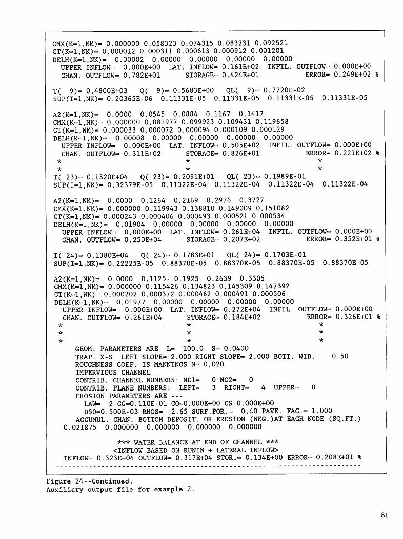
CMX(K=1,NK)= 0.000000 0.058323 0.074315 0.083231 0.092521CT(K=1,NK)= 0.000012 0.000311 0.000613 0.000912 0.001201DELH(K=1,NK)= 0.00002 0.00000 0.00000 0.00000 0.00000UPPER INFLOW- O.OOOE+00 LAT. INFLOW- 0.161E+02 INFIL. OUTFLOW- O.OOOE+00CHAN. OUTFLOW- 0.782E+01 STORAGE- 0.424E+01 ERROR- 0.249E+02 %

T( 9)= 0.4800E+03 Q( 9)- 0.5683E+00 QL( 9)= 0.7720E-02SUP(I-1,NK)= 0.20365E-06 0.11331E-05 0.11331E-05 0.11331E-05 0.11331E-05

A2(K=1,NK)= 0.0000 0.0545 0.0884 0.1167 0.1417CMX(K=1,NK)= 0.000000 0.081977 0.099923 0.109431 0.119658CT(K-1,NK)= 0.000033 0.000072 0.000094 0.000109 0.000129

0.00000

INFIL. OUTFLOW*

ERROR*

*

*

O.OOOE+00

0.221E+02 %

DELH(K=1,NK)= 0.00008 0.00000 0.00000 0.00000UPPER INFLOW- O.OOOE+00 LAT. INFLOW- 0.505E+02

CHAN. OUTFLOW- 0.311E+02 STORAGE- 0.826E+01* *

* *

T( 23)= 0.1320E+04 Q( 23)= 0.2091E+01 QL( 23)=SUP(I=1,NK)= 0.32379E-05 0.11322E-04 0.11322E-04

0.1989E-01

0.11322E-04 0.11322E-04

A2(K=1,NK)= 0.0000 0.1264 0.2169 0.2976 0.3727CMX(K=1,NK)= 0.000000 0.119943 0.138810 0.149009 0.151082CT(K-1,NK)= 0.000243 0.000406 0.000493 0.000521 0.000534DELH(K=1,NK)= 0.01904 0.00000 0.00000 0.00000 0.00000

UPPER INFLOW- O.OOOE+00 LAT. INFLOW- 0.261E+04 INFIL.

CHAN. OUTFLOW- 0.250E+04 STORAGE- 0.207E+02

OUTFLOW*

ERROR*

O.OOOE+00

0.352E+01 %

T( 24)= 0.1380E+04 Q( 24)- 0.1783E+01 QL( 24)= 0.1703E-01SUP(I-1,NK)= 0.22225E-05 0.88370E-05 0.88370E-05 0.88370E-05

A2(K=1,NK)- 0.0000 0.1125 0.1925 0.2639 0.3305CMX(K=1,NK)= 0.000000 0.115426 0.134823 0.145309 0.147392CT(K=1,NK)= 0.000202 0.000372 0.000462 0.000491 0.000506DELH(K=1,NK)= 0.01977 0.00000

UPPER INFLOW- O.OOOE+00 LAT

CHAN. OUTFLOW- 0.261E+04

*

*

*

GEOM. PARAMETERS ARE L=

TRAP. X-S LEFT SLOPE- 2.000 RIGHT SLOPE- 2.000 BOTT. WID.= 0.50ROUGHNESS COEF. IS MANNINGS N= 0.020

IMPERVIOUS CHANNEL

CONTRIB. CHANNEL NUMBERS: NCI- 0 NC2- 0

CONTRIB. PLANE NUMBERS: LEFT- 3 RIGHT- 4 UPPER- 0


LAW- 2 CG-0.110E-01 CO=0.000E+00 CS-O.000E+O0D50-0.500E-03 RHOS- 2.65 SURF.POR. = 0.40 PAVE. FAC= 1.000

ACCUMUL. CHAN. BOTTOM DEPOSIT. OR EROSION (NEG.)AT EACH NODE (SQ.FT.)0.021875 0.000000 0.000000 0.000000 0.000000



INFLOW- 0.323E+04 OUTFLOW= 0.317E+04 STOR.= 0.134E+00 ERROR- 0.208E+01 %

0.88370E-05

0.00000 0.00000 0.00000

. INFLOW- 0.272E+04 INFIL. OUTFLOW- O.OOOE+00

STORAGE- 0.184E+02 ERROR- 0.326E+01 %

* *

* *

* *

100.0 s= 0.0400


81

82

** CONDUIT NO 6 DIAGNOSTIC INFORMATION **

GEOM. PARAMETERS ARE L- 150.0 S- 0.0200

CIRCULAR SHAPE - DIAMETER - 2.00000

ROUGHNESS COEF. IS MANNINGS N- 0.012

IMPERVIOUS CHANNEL

CONTRIB. CHANNEL NUMBERS: NC1= 2 NC2- 5

CONTRIB. PLANE NUMBERS: LEFT- 0 RIGHT- 0 UPPER- 0


LAW- 2 CG-0.110E-01 CO-0.000E+00 CS-0.000E+00

D50-0.500E-03 RHOS- 2.65 SURF.POR.- 0.40 PAVE. FAC- 1.000

ACCUMUL. CHAN. BOTTOM DEPOSIT. OR EROSION (NEG.)AT EACH NODE (SQ.FT.)0.000000 0.000000 0.000000 0.000000 0.000000 0.000000 0.000000

*** WATER BALANCE AT END OF CONDUIT ***

<INFLOW BASED ON UPSTREAM RUNIN ONLY>

INFLOW- 0.478E+04 OUTFLOW- 0.478E+04 STOR.- 0.439E+00 ERROR—0.106E-01 %


During the first few time steps the plane volume balance errorsmay become as large as 10 percent, but they quickly decreaseuntil they are usually smaller than 1 percent. These errors aredue to the numerical approximation involved in estimating thestorage at each time step. When the storage is large relativeto the total inflow, the errors can be about 10 percent. Laterwhen the storage is small relative to the total inflow, theyusually become inconsequential.

Detailed printouts for channel 5 are shown at two selected timesin figure 24. At time [T(8) = 420s] the channel discharge atthe lower boundary [Q(8)] is 0.207 cubic feet per second and thelateral inflow rate [QL(8)] is 0.003767 cubic feet per secondper foot. The cross-sectional area of flow at each node isdenoted by A2(K-1,NK). This channel is nonerodible. so thesediment supply term SUP(I-1,NK) consists of the lateral inflowof sediment contributed by planes 3 and 4. The transportcapacity at the upper node is zero.so deposition is occurring.Consequently the net supply rate at node 1 is lower than thedownstream nodes and deposition is indicated by a positive DELH.The channel is nonerodible. so DELH remains zero at nodes 2through 4 although the concentration (CT) is much lower than thetransport capacity (CMX).

The purpose of the auxiliary file is to provide insight into thedetailed computations and to assist in understanding runoff anderosion dynamics as described by the algorithms used in KINEROS.In the early stages of an analysis of a particular watershed,the auxiliary file should be examined carefully, for it canreveal inconsistencies in input parameters or problems with thefinite difference schemes.

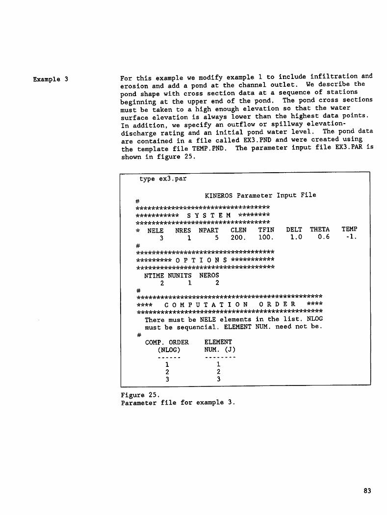
Example 3 For this example we modify example 1 to include infiltration anderosion and add a pond at the channel outlet. We describe thepond shape with cross section data at a sequence of stationsbeginning at the upper end of the pond. The pond cross sectionsmust be taken to a high enough elevation so that the watersurface elevation is always lower than the highest data points.In addition, we specify an outflow or spillway elevation-discharge rating and an initial pond water level. The pond dataare contained in a file called EX3.PND and were created usingthe template file TEMP.PND. The parameter input file EX3.PAR isshown in figure 25.

type ex3.par

#

**********************************

*********** SYSTEM ******************************************

* NELE NRES NPART CLEN TFIN DELT THETA3 1 5 200. 100. 1.0 0.6

#

***********************************

********* OPTIONS **********************************************

NTIME NUNITS NEROS

2 12

#

***********************************************


There must be NELE elements in the list. NLOGmust be sequencial. ELEMENT NUM. need not be.

#

COMP. ORDER ELEMENT

(NLOG) NUM. (J)


Figure 25.Parameter file for example 3

TEMP

-1.

83

84

#

***********************************************



J

1

NU

0

NR

0

NL

0

NCI

0

NC2

0

NCASE

0

NPRINT

1

NPNT

0

NRP

0

XL

100.0

W

200.0

S

0.05

ZR

0.0

ZL

0.0

BW

0.0

DIAM

0.0

Rl

0.013

R2

0.0

FMIN

0.068

G

10.4

POR

0.4

SI

0.25

SMAX

0.83

ROC

0.2

RECS

0.2

DINTR

0.03

*

*

J

2

LAW

3

NU

0

CF

200.0

NR

0

CG

0.02

NL

1

CH

300.0

NCI

0

CO-CS

1.0

NC2

0

D50

0.0001

NCASE

1

RHOS

2.65

NPRINT

2

PAVE

0.1

NPNT

0

SIGMAS

0.02

NRP

0

XL

200.0

W

0.0

S

0.03

ZR

1.0

ZL

1.0

BW

2.0

DIAM

0.0

Rl

0.013

R2

0.0

FMIN

4.0

G

1.8

POR

0.44

SI

0.40

SMAX

0.95

ROC

0.2

RECS

0.0

DINTR

0.0

*

*

J

3

LAW

6

NU

0

CF

0.0

NR

0

CG

0.01

NL

0

CH

0.0

NCI

2

CO-CS

0.0

NC2

0

D50

0.0001

NCASE

0

RHOS

2.65

NPRINT

2

PAVE

0.1

NPNT

1

SIGMAS

0.02

NRP

0

XL

0.0

w

0.0

S

0.0

ZR

0.0

ZL

0.0

BW

0.0

DIAM

0.0

Rl

0.0

R2

0.0

FMIN

0.0

G

0.0

POR

0.0

SI

0.0

SMAX

0.0

ROC

0.0

RECS

0.0

DINTR

0.0

*

LAW

0

CF

0.0

CG

0.0

CH

0.0

CO-CS

0.0

D50

0.0001

RHOS

2.65

PAVE

0.0

SIGMAS

0.02

Figure 25--Continued.Parameter file for example 3

Under the "SYSTEM" heading, NELE is now 3 and TFIN has beenincreased to 100 to accommodate ponding delay. NPART = 5 causesthe sediment size distribution, lognormal with mode = D50 (ft),and standard deviation = SIGMAS(NCI) to be represented by fiveequal volume parts, each represented by a mean sediment sizecalculated by the program. Under "OPTIONS, NEROS = 2 to allowerosion. The pond, element 3, has been added to NLOG. Thegeometries of elements 1 and 2 are the same as those for example1, and the erosion parameters are identical to those in example2, except that for plane 1 we have entered values for CF (200),CG (0.02), CS (1.0), and D50 (0.0001) and for channel 2 valuesfor CG (0.01) and D50 (0.0001). Infiltration has been allowedin channel 2 by setting FMIN = 4.0, G = 1.8, SMAX - 0.95, POR -0.44, and SI = 0.40. Data for the pond element 3 are added.NCI = 2 indicates that channel 2 contributes to the pond. NPNT= 1 signifies that this is a pond element and that the pondgeometry data must be read. The pond data file is shown infigure 26.

NPND will correspond to NPNT in the parameter file (1, 2, or 3).In this example, there is only one pond, so NPND = 1. NSEC isthe number of cross section locations (4). MEL is the number ofelevations at which cross-sectional areas (A) and top widths(TWP) are given. ELST is the water surface elevation at thebeginning of the simulation (101.0 ft). ELVZ is the elevationof the lowest point on the pond bottom (100.0 ft). TDIFUS isthe diffusion coefficient for pond mixing, specified as 0.0005

ft2/s.

The NSEC (4) cross sections are at 0.0, 5.0, 10.0, and 20.0 ft(XSEC) from the upper end of the pond. NOPQ is 4, the number ofstage-discharge pairs for the pond rating table, and ELZQ is thelowest elevation at which outflow begins (102.0 ft). ELQ and

3QSO are the elevations and discharges (ft /s) for the outflowrating table. Note that a very small value of discharge must beentered at ELZQ because logarithmic interpolation is used toestimate discharge between tabulated values.

Cross-sectional areas and widths are specified at MEL(5)elevations: 101., 102., 103 , 104., and 105. ft. If the minimumelevation at that section is greater than the tabulatedelevation, A and TWP are set to zero. The rainfall input dataare printed (fig. 27) as are the hydrograph and sedigraph data(fig. 28). From the summary information in figure 28 we seethat 223 pounds of sediment have been deposited in the pond.

85

86

type ex3.pnd

KINEROS Pond Input Data1)#

#

#

#

#

****************************

Pond Cross-section Layout****************************

POND NUM. OF NUM. OF ELEV,

NUMB. POND X-S IN POND X-S

(NPND) (NSEC) (MEL)

NOTE: If more then one pond exists the entire block of lines fromline one (1) to the * line after the last X-S must be repeatedwith appropriate input values corresponding to that pond.

#

BEG. POND

ELEVATION

(ELST)

101.0

LOWEST ELEV.

OF POND

(ELVZ)

100.0

POND DIFFUS.

COEF. (FT**2/S)(TDIFUS)

0.0005

Enter the pairs of X-S number and the distance from the upper end ofthe pond (XSEC) to the associated cross section.

X-S NUM DIST. TO X-S

(XSEC)

1 0.02 5.0

3 10.0

4 20.0

#

**********************************

* Outflow Rating Table ***********************************

NUM. OF ELEV. OF ZERO

DEPTH-FLOW PAIRS FLOW

(NOPQ) (ELZQ)

#

102.0

Enter (NOPQ) elevation (ELQ) - discharge (QSO) pairs.NOTE: The first elevation must - ELZQ and have

(1.0E-10) discharge associated with it.(ELQ) (QSO)

102. 1.0E-10

103. 5.0

104. 25.0

105. 130.0

*********************************

Specific Cross-section Data*********************************

There must be (NSEC) sets of cross-section records with (MEL) elevationsper X-S with X-S area (A) and top width (TWP). For each cross-sectionrepeat lines from * to * inserting the appropriate num. of elev. (MEL)****

NOTE: The pond cross section information must be defined to the "same"**** elev. as the highest elev. in the elevation-discharge table.

Figure 26.Pond geometry for example 3.

*

X-S NUM. ELEV. X -S AREA X-S TOP WIDTH

1

(EL)

101.0

(A) (TWP)

0.0 0.0

1 102.0 0.0 0.0

1 103.0 1.0 3.15

1 104.0 6.23 7.33

*

1 105.0 10.30 9.58

*


2

(EL)

101.0

(A) (TWP)

0.0 0.0

2 102.0 0.46 2.11

2 103.0 6.51 8.41

2 104.0 16.20 11.31

*

2 105.0 28.80 15.49

*


3

(EL)

101.0

(A) (TWP)

1.52 3.053 102.0 7.49 9.24

3 103.0 21.10 14.30

3 104.0 36.30 17.70

*

3 105.0 52.75 22.45

*


4

(EL)

101.0

(A) (TWP)

1.71 4.22

4 102.0 7.30 6.574 103.0 15.20 10.70

4 104.0 30.50 21.10

4 105.0 44.30 27.70*

Figure 26--Continued.Pond geometry for example 3

87

88

type ex3.pre


****************************


#

NUM. OF RAINGAGES MAX. NUM. OF TIME-DEPTH DATA PAIRS FOR ALL GAGES

(NGAGES) (MAXND)

#

There must be NELE pairs of (GAGE WEIGHT) data.

ELE. NUM. (J)

1

2

3

#

*****************************

Rainfall Data*****************************


#

* ALPHA-NUMERIC GAGE ID: EXAMPLE 1 - GAGE 1 = GAGE 1.#


RAINGAGE

1

1

1

WEIGHT

1.0

1.0

1.0


TIME ACCUM. DEPTH

0.0 0.0

5.0 0.210.0 0.6

20.0 1.0150.0 1.0

Figure 27.Rainfall file for example 3.

type ex3.dat

INPUT POND FILE: EX3.PND



===== DESCRIPTIVE RUN TITLE —


VOL. BAL. SED. TOTAL

ELE #

1

TYPE

PLANE

ERROR % (LBS.)

-0.182E-01 412.324

2 CHANNEL 0.398E+00 473.014

3 POND -0.106E+01 250.353


CONTRIBUTING AREA= 20000.000 SQ. FEET OR 0.45913681 ACRES


0.00 0.00000 0.000000 0.00000000 0.OOOOE+00

1.00 0.00000 0.000000 0.00000000 0.OOOOE+00

2.00 0.00000 0.000000 0.00000000 0.0000E+00

3.00 0.00000 0.000000 0.00000000 0.0000E+00

4.00 0.00000 0.000000 0.00000000 0.OOOOE+00

5.00 0.00000 0.000000 0.00000000 0.OOOOE+00

6.00 0.00000 0.000000 0.00000000 0.OOOOE+00

7.00 0.60293 1.302334 0.00000000 0.OOOOE+00

8.00 1.71459 3.703523 0.00214861 2.388

9.00 1.85484 4.006453 0.00380759 4.578

10.00 1.83688 3.967661 0.00278809 3.320

11.00 1.64615 3.555693 0.00139102 1.484

12.00 1.17935 2.547404 0.00099808 0.7631* * * * *

* * * * *

97.00 0.00002 0.000050 0.00024885 0.3723E-05

98.00 0.00002 0.000050 0.00024735 0.3701E-05

99.00 0.00002 0.000050 0.00024591 0.3679E-05

100.00 0.00002 0.000050 0.00024453 0.3658E-05

TIME TO PEAK FLOW RATE = 9.0000 (MIN)PEAK FLOW RATE 4.0065 (IPH)

* *** EVENT SUMMARY ****

Figure 28.Parts of output file for example 3

89

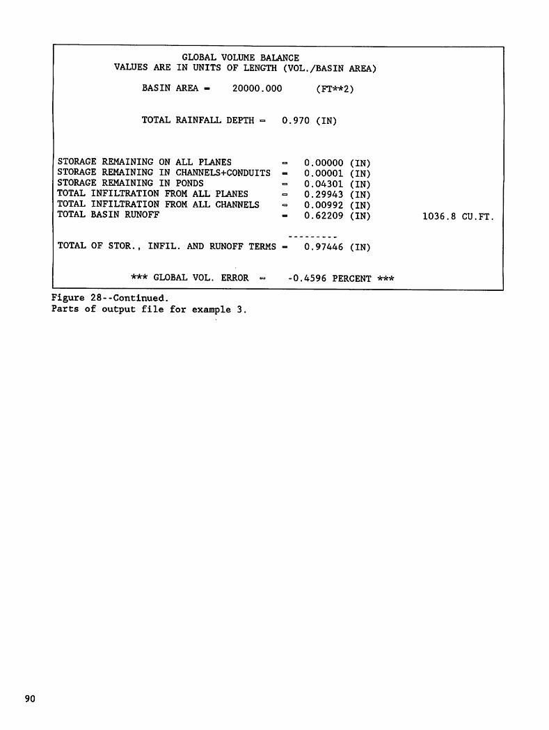
90



BASIN AREA 20000.000 (FT**2)

TOTAL RAINFALL DEPTH






TOTAL BASIN RUNOFF

TOTAL OF STOR., INFIL. AND RUNOFF TERMS

*** GLOBAL VOL. ERROR

Figure 28--Continued.Parts of output file for example 3

0.970 (IN)

0.00000 (IN)0.00001 (IN)0.04301 (IN)0.29943 (IN)0.00992 (IN)0.62209 (IN)

0.97446 (IN)

•0.4596 PERCENT ***

1036.8 CU.FT

EXAMPLES USING REAL WATERSHEDS

Applications of previous versions of KINEROS have beendemonstrated by Rovey et al. (1977), Rovey and Woolhiser (1977),Smith (1981), Osborn et al. (1982). and Wheater and Bell (1983);but a thorough validation has not been accomplished. Such astudy should include data from several watersheds and comparisonof observed and predicted hydrographs where (1) all parametershave been estimated a priori or (2) all parameters had beenestimated from data not included in the prediction set, that is,split-sample tests. We do not intend to present such a study inthis manual. However, examples 4 and 5 deal with realwatersheds, and parameters were selected from the physicalcharacteristics of the watersheds based on information providedin this manual.

Example 4 For this example, we have created a data file for Lucky HillsWatershed, LH106, a small (0.864 acre) subwatershed in theWalnut Gulch Experimental Watershed in southeastern Arizona.Watershed 106 has been instrumented since 1965. It was treated

with a brush-killing chemical (Tebuthiuron) in 1981 and wasreseeded with grasses and forbs in 1984. We wish to use KINEROSto investigate the effects of these dramatic changes invegetative cover, so we provide a detailed geometricrepresentation. The procedures used to develop the cascade ofplanes and channels are applicable to larger areas, although thegeometric detail in this example is much greater.

A topographic map of the watershed is shown in figure 29A.Using a tracing paper overlay, the channel system was traced,and the areas contributing to each channel were outlined bydrawing dashed lines at right angles to the contours. Eachfirst order channel has three contributing areas, onecontributing to the upper end of the channel and one areacontributing to each side of the channel (see fig. 29B). Thereare seven channel segments including one segment to add theoutflow from the two tributaries that join above the measuringflume. There are 4 first order channels that require a minimumof 12 planes and 3 higher order channels that require a minimumof 6 planes. Therefore, the geometric representation requires aminimum of 25 elements. Identifying numbers were assigned toeach channel element and are shown circled in figure 29B. It is•useful to assign these numbers in the order that the flow in thechannels will be calculated.

91

FlumeArea =3490m

Contour interval: | foot(0.3048m)

Relative datum

Scale in

20

B

Element boundary•—*• Channels

@ Channel element number[9) Plane element number

Figure 29.

Watershed LH106: A, topographic map; B, division into planes and channels

92

Next, flow lines are drawn beginning at the midpoint of eachchannel and at the end of the first order channels toward the

divide. These flow lines should be as long as the visuallyestimated average length of flow in the contributing area. Thetopographic profiles along these lines should be examined forsignificant changes of slope, and if a change (or changes) isdetected, the contributing area should be segmented into morethan one plane. For example, the area contributing to the leftside of channel 3 has a uniform slope, so only one plane isrequired. The length of this plane is equal to the length ofthe flow line that has been drawn. The width is equal to thecontributing area divided by the length. The slope wascalculated by dividing the total difference in elevation alongthe flow line by the length of the plane. There is a break inslope along the flow line drawn within the area contributing tothe left side of channel 1. Therefore, a line was drawn throughthe break in slope and approximately parallel to the channel.Plane numbers are shown in boxes on figure 29B.

Convergence such as that exhibited in the area contributing tothe upper end of channel 1 may require the use of more than oneplane. A change in soil type may also require furthersubdivision. For this watershed, soil characteristics areclosely related to position on the slope, with highly erodedsoils on the steep slopes, so no further delineation of subareaswill be required. The total number of elements NELE = 30 isentered in the parameter file LH106.PAR (fig. 30). Because thisis a natural watershed we selected the Manning resistance law(NRES = 1).

type lhl06.par

TYPE-W-SEARCHFAIL, error searching for LH106.PAR-RMS-F-SYN, file specification syntax error

type lhl06.par


**********************************

*********** SYSTEM ********

**********************************

* NELE NRES NPART CLEN TFIN

30 1 0 148. 150,#

***********************************

********* OPTIONS ***********

***********************************

NTIME NUNITS NEROS

2 11

DELT THETA

0.5 0.8

***********************************************




COMP. ORDER ELEMENT

(NLOG) NUM. (J)

1 10

2 8

3 9

4 11

5 1

6 12

7 13

8 14

9 15

10 2

11 16

12 17

13 3

14 24

15 25

16 26

17 27

18 28

19 4

20 20

21 21

22 22

23 23

24 5

25 29

Figure 30.Parameter input file for example 4,

TEMP

-1.

93

94

26 30

27 6

28 18

29 19

30 7

#

***********************************************

****** E L E M E: N T - W I S E IN F 0 ***

***********************************************

There must be NELE setsi of the ELEMENT-WISE prompts and datarecords; duplicate records from * to * for each element . The

*

J

elements may t>e entered in any order.

NU NR NL NCI NC2 NCASE NPRINT NPNT NRP

1 10 11 9 0 0 1 1 0 0


116. 0.0 .13 .159 .159 0.5 0. .02 0.

FMIN G POR SI SMAX ROC RECS DINTR

0.0 0.0 .0 .0 0 0 0. 0.


*

0 0 0 0 0 0 0 0 0

*

J NU NR NL NCI NC2 NCASE NPRINT NPNT NRP

2 12 15 14 0 0 1 1 0 0


85 0.0 .085 .159 .159 0.5 0. .02 0.


.0 0.0 0.0 .00 0 0 0.00 0.


*

0 0 0 0 0 0 0 0 0

*


3 0 17 16 1 2 1 1 0 0


73 0.0 .062 .37 .37 0.5 0. .02 0.


.0 0.0 0.0 .00 0 0 0.00 0.


*

0 0 0 0 0 0 0 0 0

*


4 24 28 26 0 0 1 1 0 0

Figure 30--Continued.Parameter input file for example 4

XL

89

W

0.0

S

.069

ZR

.14

ZL

.14

BW

0.5

DIAM

0.

Rl

.02

R2

0.

FMIN

.0

G

0.0

POR

0.0

SI

.00

SMAX

0

ROC

0

RECS

0.00

DINTR

0.

*

*

J

5

LAW

0

NU

21

CF

0

NR

23

CG

0

NL

22

CH

0

NCI

0

CO-CS

0

NC2

0

D50

0

NCASE

1

RHOS

0

NPRINT

1

PAVE

0

NPNT

0

SIGMAS

0

NRP

0

XL

27

W

0.0

S

.11

ZR

.087

ZL

.087

BW

0.5

DIAM

0.

Rl

.02

R2

0.

FMIN

.0

G

0.0

POR

0.0

SI

.00

SMAX

0

ROC

0

RECS

0.00

DINTR

0.

*

*

J

6

LAW

0

NU

0

CF

0

NR

30

CG

0

NL

29

CH

0

NCI

4

CO-CS

0

NC2

5

D50

0

NCASE

1

RHOS

0

NPRINT

1

PAVE

0

NPNT

0

SIGMAS

0

NRP

0

XL

79

W

0.0

S

.075

ZR

.212

ZL

.212

BW

0.5

DIAM

0.

Rl

.02

R2

0.

FMIN

.0

G

0.0

POR

0.0

SI

.00

SMAX

0

ROC

0

RECS

0.00

DINTR

0.

*

*

J

7

LAW

0

NU

0

CF

0

NR

19

CG •

0

NL

18

CH

0

NCI

6

CO-CS

0

NC2

3

D50

0

NCASE

1

RHOS

0

NPRINT

1

PAVE

0

NPNT

0

SIGMAS

0

NRP

0

XL

15

W

0.0

S

.067

ZR

1.0

ZL

1.0

BW

0.5

DIAM

0.

Rl

.02

R2

0.

FMIN

.0

G

0.0

POR

0.0

SI

.00

SMAX

0

ROC

0

RECS

0.00

DINTR

0.

*

*

J

8

LAW

0

NU

0

CF

0

NR

0

CG

0

NL

0

CH

0

NCI

0

CO-CS

0

NC2

0

D50

0

NCASE

0

RHOS

0

NPRINT

1

PAVE

0

NPNT

0

SIGMAS

0

NRP

0

XL

80

w

52

S

.08

ZR

0.

ZL

0.

BW

0

DIAM

0.

Rl

.03

R2

0.


95

96

FMIN

0.31

G

5.00

POR

.453

SI

0.2

SMAX

0.91

ROC

.40

RECS

0.36

DINTR

0.

*

*

J

9

LAW

0

NU

8

CF

0

NR

0

CG

0

NL

0

CH

0

NCI

0

CO-CS

0

NC2

0

D50

0

NCASE

0

RHOS

0

NPRINT

1

PAVE

0

NPNT

0

SIGMAS

0

NRP

0

XL

68

W

56.5

S

.11

ZR

0.

ZL

0.

BW

0.

DIAM

0.

Rl

.03

R2

0.

FMIN

0.28

G

5.00

POR

.453

SI

0.2

SMAX

0.91

ROC

.445

RECS

0.36

DINTR

0.

*

*

J

10

LAW

0

NU

0

CF

0

NR

0

CG

0

NL

0

CH

0

NCI

0

CO-CS

0

NC2

0

D50

0

NCASE

0

RHOS

0

NPRINT

1

PAVE

0

NPNT

0

SIGMAS

0

NRP

0

XL

51

W

23.5

S

.078

ZR

0.

ZL

0.

BW

0.

DIAM

0.

Rl

.03

R2

0.

FMIN

0.31

G

5.00

POR

.453

SI

0.2

SMAX

0.91

ROC

.40

RECS

0.36

DINTR

0.

*

*

J

11

LAW

0

NU

0

CF

0

NR

0

CG

0

NL

0

CH

0

NCI

0

CO-CS

0

NC2

0

D50

0

NCASE

0

RHOS

0

NPRINT

1

PAVE

0

NPNT

0

SIGMAS

0

NRP

0

XL

72

w

39

S

.10

ZR

0.

ZL

0.

BW

0.

DIAM

0.

Rl

.03

R2

0.

FMIN

0.28

G

5.00

POR

.453

SI

0.2

SMAX

0.91

ROC

.445

RECS

0.36

DINTR

0.

*

*

J

12

LAW

0

NU

0

CF

0

NR

0

CG

0

NL

0

CH

0

NCI

0

CO-CS

0

NC2

0

D50

0

NCASE

0

RHOS

0

NPRINT

1

PAVE

0

NPNT

0

SIGMAS

0

NRP

0

XL

88

W

17

S

.07

ZR

0.

ZL

0.

BW

0.

DIAM

0.

Rl

.03

R2

0.

FMIN

0.31

G

5.00

POR

.453

SI

0.2

SMAX

0.91

ROC

.40

RECS

0.36

DINTR

0.


*

LAW

0

CF

0

CG

0

CH

0

CO-CS

0

D50

0

RHOS

0

PAVE

0

SIGMAS

0

*

J

13

NU

0

NR

0

NL

0

NCI

0

NC2

0

NCASE NPRINT

0 1

NPNT

0

NRP

0

XL

63

w

29

S

.06

ZR

0.

ZL

0.

BW

0.

DIAM

0.

Rl

.03

R2

0.

FMIN

0-.31

G

5.00

POR

.453

SI

0.2

SMAX

0.91

ROC

.40

RECS

0.36

DINTR

0.

*

LAW

0

CF

0

CG

0

CH

0

CO-CS

0

D50

0

RHOS

0

PAVE

0

SIGMAS

0

*

J

14

NU

13

NR

0

NL

0

NCI

0

NC2

0

NCASE

0

NPRINT

1

NPNT

0

NRP

0

XL

27

w

59

S

.11

ZR

0.

ZL

0.

BW

0.

DIAM

0.

Rl

.03

R2

0.

FMIN

0.28

G

5.00

POR

.453

SI

0.2

SMAX

0.91

ROC

.445

RECS

0.36

DINTR

0.

*

LAW

0

CF

0

CG

0

CH

0

CO-CS

0

D50

0

RHOS

0

PAVE

0

SIGMAS

0

*

J

15

NU

0

NR

0

NL

0

NCI

0

NC2

0

NCASE

0

NPRINT

1

NPNT

0

NRP

0

XL

20

W

48

S

.10

ZR

0.

ZL

0.

BW

0.

DIAM

0.

Rl

.03

R2

0.

FMIN

0.28

G

5.00

POR

.453

SI

0.2

SMAX

0.91

ROC

.445

RECS

0.36

DINTR

0.

*

LAW

0

CF

0

CG

0

CH

0

CO-CS

0

D50

0

RHOS

0

PAVE

0

SIGMAS

0

*

J

16

NU

0

NR

0

NL

0

NCI

0

NC2

0

NCASE

0

NPRINT

1

NPNT

0

NRP

0

XL

34

W

49

S

.13

ZR

0.

ZL

0.

BW

0.

DIAM

0.

Rl

.03

R2

0.

FMIN

0.36

G

5.00

POR

.453

SI

0.2

SMAX

0.91

ROC

.296

RECS

0.36

DINTR

0

*

LAW

0

CF

0

CG

0

CH

0

CO-CS

0

D50

0

RHOS

0

PAVE

0

SIGMAS

0


97

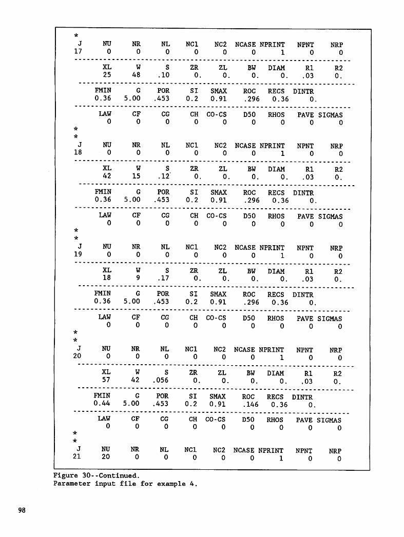
98

*

J

17

NU

0

NR

0

NL

0

NCI

0

NC2

0

NCASE

0

NPRINT

1

NPNT

0

NRP

0

XL

25

W

48

S

.10

ZR

0.

ZL

0.

BW

0.

DIAM

0.

Rl

.03

R2

0.

FMIN

0.36

G

5.00

POR

.453

SI

0.2

SMAX

0.91

ROC

.296

RECS

0.36

DINTR

0.

*

LAW

0

CF

0

CG

0

CH

0

CO-CS

0

D50

0

RHOS

0

PAVE

0

SIGMAS

0

*

J

18

NU

0

NR

0

NL

0

NCI

0

NC2

0

NCASE

0

NPRINT

1

NPNT

0

NRP

0

XL

42

W

15

S

.12'ZR

0.

ZL

0.

BW

0.

DIAM

0.

Rl

.03

R2

0.

FMIN

0.36

G

5.00

POR

.453

SI

0.2

SMAX

0.91

ROC

.296

RECS

0.36

DINTR

0.

*

LAW

0

CF

0

CG

0

CH

0

CO-CS

0

D50

0

RHOS

0

PAVE

0

SIGMAS

0

*

J

19

NU

0

NR

0

NL

0

NCI

0

NC2

0

NCASE

0

NPRINT

1

NPNT

0

NRP

0

XL

18

W

9

S

.17

ZR

0.

ZL

0.

BW

0.

DIAM

0.

Rl

.03

R2

0.

FMIN

0.36

G

5.00

POR

.453

SI

0.2

SMAX

0.91

ROC

.296

RECS

0.36

DINTR

0.

*

LAW

0

CF

0

CG

0

CH

0

CO-CS

0

D50

0

RHOS

0

PAVE

0

SIGMAS

0

*

J

20

NU

0

NR

0

NL

0

NCI

0

NC2

0

NCASE

0

NPRINT

1

NPNT

0

NRP

0

XL

57

W

42

S

.056

ZR

0.

ZL

0.

BW

0.

DIAM

0.

Rl

.03

R2

0.

FMIN

0.44

G

5.00

POR

.453

SI

0.2

SMAX

0.91

ROC

.146

RECS

0.36

DINTR

0.

*

LAW

0

CF

0

CG

0

CH

0

CO-CS

0

D50

0

RHOS

0

PAVE

0

SIGMAS

0

*

J

21

NU

20

NR

0

NL

0

NCI

0

NC2

0

NCASE ]

0

NPRINT

1

NPNT

0

NRP

0

Figure 30--Continued.Parameter input file for example 4,

1

XL

56

W

15.7

S

.07

ZR

0.

ZL

0.

BW

0.

DIAM

0.

Rl

.03

R2

0.

FMIN

0.35

G

5.00

POR

.453

SI

0.2

SMAX

0.91

ROC

.314

RECS

0.36

DINTR

0.

*

LAW

0

CF

0

CG

0

CH

0

CO-CS

0

D50

0

RHOS

0

PAVE

0

SIGMAS

0

*

J

22

NU

0

NR

0

NL

0

NCI

0

NC2

0

NCASE NPRINT

0 1

NPNT

0

NRP

0

XL

58

W

11

S

.08

ZR

0.

ZL

0.

BW

0.

DIAM

0.

Rl

.03

R2

0.

FMIN

0.35

G

5.00

POR

.453

SI

0.2

SMAX

0.91

ROC

.314

RECS

0.36

DINTR

0.

*

LAW

0

CF

0

CG

0

CH

0

CO-CS

0

D50

0

RHOS

0

PAVE

0

SIGMAS

0

*

J

23

NU

0

NR

0

NL

0

NCI

0

NC2

0

NCASE

0

NPRINT

1

NPNT

0

NRP

0

XL

74

W

19

S

.09

ZR

0.

ZL

0.

BW

0.

DIAM

0.

Rl

.03

R2

0.

FMIN

0.35

G

5.00

POR

.453

SI

0.2

SMAX

0.91

ROC

.314

RECS

0.36

DINTR

0.

*

LAW

0

CF

0

CG

0

CH

0

CO-CS

0

D50

0

RHOS

0

PAVE

0

SIGMAS

0

*

J

24

NU

0

NR

0

NL

0

NCI

0

NC2

0

NCASE

0

NPRINT

1

NPNT

0

NRP

0

XL

82

W

14

S

.028

ZR

0.

ZL

0.

BW

0.

DIAM

0.

Rl

.03

R2

0.

FMIN

0.44

G

5.00

POR

.453

SI

0.2

SMAX

0.91

ROC

.146

RECS

0.36

DINTR

0.

*

LAW

0

CF

0

CG

0

CH

0

CO-CS

0

D50

0

RHOS

0

PAVE

0

SIGMAS

0

*

J

25

NU

0

NR

0

NL

0

NCI

0

NC2

0

NCASE

0

NPRINT

1

NPNT

0

NRP

0

XL

79

W

22

S

.04

ZR

0.

ZL

0.

BW

0.

DIAM

0.

Rl

.03

R2

0.

Figure 30--Continued.Parameter input file for example 4.

99

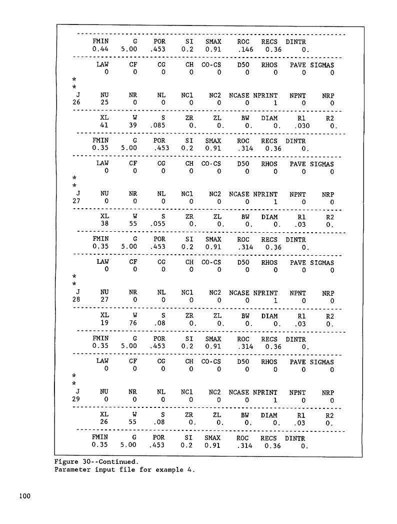
100

FMIN

0.44

G

5.00

POR

.453

SI

0.2

SMAX

0.91

ROC

.146

RECS

0.36

DINTR

0.

*

*

J

26

LAW

0

NU

25

CF

0

NR

0

CG

0

NL

0

CH

0

NCI

0

CO-CS

0

NC2

0

D50

0

NCASE

0

RHOS

0

NPRINT

1

PAVE

0

NPNT

0

SIGMAS

0

NRP

0

XL

41

W

39

S

.085

ZR

0.

ZL

0.

BW

0.

DIAM

0.

Rl

.030

R2

0.

FMIN

0.35

G

5.00

POR

.453

SI

0.2

SMAX

0.91

ROC

.314

RECS

0.36

DINTR

0.

*

*

J

27

LAW

0

NU

0

CF

0

NR

0

CG

0

NL

0

CH

0

NCI

0

CO-CS

0

NC2

0

D50

0

NCASE

0

RHOS

0

NPRINT

1

PAVE

0

NPNT

0

SIGMAS

0

NRP

0

XL

38

w

55

S

.055

ZR

0.

ZL

0.

BW

0.

DIAM

0.

Rl

.03

R2

0.

FMIN

0.35

G

5.00

POR

.453

SI

0.2

SMAX

0.91

ROC

.314

RECS

0.36

DINTR

0.

*

*

J

28

LAW

0

NU

27

CF

0

NR

0

CG

0

NL

0

CH

0

NCI

0

CO-CS

0

NC2

0

D50

0

NCASE

0

RHOS

0

NPRINT

1

PAVE

0

NPNT

0

SIGMAS

0

NRP

0

XL

19

W

76

S

.08

ZR

0.

ZL

0.

BW

0.

DIAM

0.

Rl

.03

R2

0.

FMIN

0.35

G

5.00

POR

.453

SI

0.2

SMAX

0.91

ROC

.314

RECS

0.36

DINTR

0.

*

*

J

29

LAW

0

NU

0

CF

0

NR

0

CG

0

NL

0

CH

0

NCI

0

CO-CS

0

NC2

0

D50

0

NCASE 1

0

RHOS

0

NPRINT

1

PAVE

0

NPNT

0

SIGMAS

0

NRP

0

XL

26

W

55

S

.08

ZR

0.

ZL

0.

BW

0.

DIAM

0.

Rl

.03

R2

0.

FMIN

0.35

G

5.00

POR

.453

SI

0.2

SMAX

0.91

ROC

.314

RECS

0.36

DINTR

0.


*

LAW

0

CF

0

CG

0

CH

0

CO-CS

0

D50

0

RHOS

0

PAVE

0

SIGMAS

0

*

J

30

NU

0

NR

0

NL

0

NCI

0

NC2

0

NCASE

0

NPRINT

1

NPNT

0

NRP

0

XL

38.W

34

S

.10

ZR

0.

ZL

0.

BW

0.

DIAM

0.

Rl

.03

R2

0.

FMIN

0.36

G

5.00

POR

.453

SI

0.2

SMAX

0.91

ROC

.296

RECS

0.36

DINTR

0.

*

LAW

0

CF

0

CG

0

CH

0

CO-CS

0

D50

0

RHOS

0

PAVE

0

SIGMAS

0


The longest total length of overland flow is found in the areascontributing to the left side of channel 1, so thecharacteristic length CLEN equals the sum of the lengths ofplanes 8 and 9 or 148 ft. The rainfall event lasted a total of96 min, so TFIN - 150. The variable DELT, which is the fixedtime step, will vary with the length, slope, and hydraulicresistance of planes and channels and with the rate of lateralinflow. An approximate value can be obtained from the relation

DTCLEN (n)

1.49 S1/2fQI - FMINl([ max J

I V5

2/3

for the Manning equation (in English units) or

DT =^ CLEN

-,2/3

C S1/2[QImax

FMIN1/2

[48

49]

for the Chezy equation, where QI is the maximum rainfall ratemax

for the event. According to equations [48] and [49], DT ischosen to equal 0.20 of the kinematic time to equilibrium for aplane of length (CLEN) and slope (S) with rainfall excess equalto QI - FMIN.

max

101

102

For this example

0.6

™ 1 jDT - - «

148 (0.03-)

1.49 (0.10)°*5[(4.2- 0.3)/43,200]°*66732 s [50]

Therefore DELT =0.5 min.

THETA is the weighting factor in the finite difference equationsfor overland and channel flow. We use a value of 0.8.

TEMP is the water temperature [65°F]. For options description,NTIME = 2, indicating time in minutes, NUNITS = 1 indicatingEnglish units, and NEROS = 1 indicating that erosioncomputations will not be made.

The order of calculation can occur in many ways, but in generalthe calculations can begin on either the area tributary tochannel 3 or the area tributary to channel 6. For this example,we start with element 10, a tributary of channel 3. Thecalculation sequence is entered into the file LH106.PAR. Theparameters for position in system, output options, geometry,hydraulic resistance, and infiltration are entered into theappropriate elementwise descriptions for each plane element.

Watershed 106 was originally covered with sparse brush, mostlywhitethorn and creosote bush, with bare areas between. Theseareas have an erosion pavement covering approximately 40 percentof the area. From table 4 a Manning's n of 0.03 was estimatedfor all plane elements. Therefore the parameter Rl was set to0.03 for all planes.

Infiltration Parameters

Soil samples at 0- to 5-cm and 5- to 10-cm depths were taken atsix sites at LH106 and were analyzed for percent rock, sand,silt, and clay. Rock was taken as the fraction not passing a2-mm sieve. Infiltration parameters G, POR, SMAX, FMIN, and ROCwere assigned to each plane based on the texturalcharacteristics of the sample from 0-5 cm at the nearestsampling point.

The textural classification of the surface soil for alllocations was sandy loam. From table 2 we selected the valuesof G, POR, and K as 5.0, 0.453, and 1.0 in/h, respectively.

The parameter G will be corrected for the rock fraction by theprogram. Therefore G is 5.0 for all planes. Kg, however,

should be corrected for volume of rock and for air entrapment

before it is entered as FMIN. To correct K , it was firsts

divided by 2 to approximate K under imbibition; then it was

multiplied by the factor (1-ROC) to correct for the rockfraction. The rock fraction (R ) is expressed in fraction by

weight. This was converted to volume fraction (Pr) by the

relationship

Pr

1 + 1.65

l-R ^ -1r

Rr

[51]

To derive this expression it was assumed that the specificgravity of rock is 2.65 and the bulk density of the soil matrix

is 100 lb/ft3. ROC is equivalent to P in this expression; thefraction of rock from the nearest sample was used for eachplane. A typical value for SMAX, the maximum volumetric watercontent achieved under imbibition, is 0.91, so this value wasentered for each plane. The initial volumetric water contentmay range from the residual relative saturation (Sr in table 2)to SMAX. We assumed a relatively dry initial condition and setSI - 0.20 for all planes. Finally, the parameter RECS wasestimated for the planes. This parameter controls theproportion of the area of a plane in which infiltration bysurface water continues after rainfall stops. Its value shouldbe related to the surface microtopography, with a very smallvalue of RECS (not zero) representing a hydraulically smoothsurface and a larger value representing a rilled surface. RECShas units of length. If we assume that the plane surface iscompletely covered with water when the average depth is 0.03 ft,then RECS - 0.36 in.

Channel Parameters

The channels in watershed 106 are incised and do not havesignificant deposits of sand in the bottom. Because of this,infiltration rates should be very close to the rates on adjacentplanes, and infiltration in the channels themselves can beignored. Therefore, FMIN was set to zero for all channelelements. The length of the channel (XL) was scaled from themap and the element width (W) was set to zero to indicate thatthis element is a channel. The slope (S) was estimated from themap. The channel cross sections were obtained in the field bymeasuring the bottom width (BW) and the side slopes (ZL and ZR).Manning's n for the channels was estimated as 0.02 and is shownas Rl.

103

104

Rainfall Information

Rainfall information was entered into the file LH106P3.PRE (fig.31). A rainfall event that occurred on August 23, 1982, wasused for this example. Rainfall was measured on a weighingrecording raingage designated as gage 83, located adjacent tothe watershed. Thus, NGAGES = 1 for this example. Thevariables WEIGHT and RAINGAGE are required inputs. WEIGHTrefers to the relative depth of total rainfall at RAINGAGE thatfell on ELEMENT(J). Because we have only one raingage, bothWEIGHT and RAINGAGE are 1 for all 30 watershed elements.RAINGAGE must be from 1 to NGAGES. A note may be added in thedata showing equivalence of watershed gage number (83) toRAINGAGE(l). MAXND refers to the maximum number of time depthpairs that appear in the following rainfall data. In this caseMAXND = 26.

Entries under ACCUM.DEPTH represent the accumulated rain depthcorresponding to the TIME sequence. ACCUM.DEPTH begins at zeroand the last two entries are equal, indicating the end ofaccumulation and representing the total rainfall. Note that thelast time must be greater than TFIN, so that rainfallintensities are defined up to TFIN. ND refers to the number oftime depth pairs for each raingage (so with multiple gages,MAXND is the largest ND value).

Checking Parameter Files

With the detailed representation used to describe watershedLH106, it is easy to make mistakes in setting up the flow logicor entering data into the parameter file. It is an excellentpractice to check the logic by creating one file with animpervious watershed, that is, FMIN =0.0 for all elements, andto create an input rainfall file with a constant intensity (forexample, 1.0 in/h) and a duration longer than the basin time toequilibrium. If the output hydrograph approaches a steady staterate nearly equal to the input rate, all elements arecontributing and numerical errors are acceptable. If the outputhydrograph approaches a lower rate, it is likely that theparameter NU has been incorrectly set to zero for some plane orthat NU, NCI, NC2, NL, or NR has been incorrectly set to zerofor a channel element.

Output Files

Summary information on each plane and channel and the computedhydrograph are written to LH106P3.DAT, part of which is shown infigure 32. The computed and observed hydrographs from channel 7for the event of August 23, 1982, are shown in figure 33.Although there are differences between the hydrographs,agreement is fairly good considering;that all parameters wereestimated a priori. No adjustments have been made to calibratethe model results to measured data.

type Ihl06p3.pre


****************************

Gage Network Data RAIN EVENT OF 8-23-82: GAGE 83****************************

#

NUM. OF RAINGAGES MAX. NUM. OF TIME-DEPTH DATA PAIRS FOR ALL GAGES(NGAGES) (MAXND)

1 26


ELE. NUM. (J) RAINGAGE WEIGHT

1 1 1.0

2 1 1.0

3 1 1.0

4 1 1.0

5 1 1.0

6 1 1.0

7 1 1.0

8 1 1.0

9 1 1.0

10 1 1.0

11 1 1.0

12 1 1.0

13 1 1.0

14 1 1.0

15 1 1.0

16 1 1.0

17 1 1.0

18 1 1.0

19 1 1.0

20 1 1.0

21 1 1.0

22 1 1.0

23 1 1.0

24 1 1.0

25 1 1.0

26 1 1.0

27 1 1.0

28 1 1.0

29 1 1.0

30 1 1.0

#

****************************

Rainfall Data*****************************


Figure 31.Rainfall data for example 4

105

106

* ALPHA-NUMERIC GAGE ID: WALNUT GULCH GAGE #83 = GAGE NUM. 1#


1 26#


TIME ACCUM. DEPTH

0.0 0.00

4.0 0.02

6.0 0.11

11.0 0.27

15.0 0.34

17.0 0.42

20.0 0.49

23.0 0.59

28.0 0.67

34.0 0.74

42.0 0.75

49.0 0.79

51.0 0.84

54.0 0.87

57.0 0.92

61.0 0.94

66.0 0.95

69.0 0.97

73.0 1.01

77.0 1.08

81.0 1.10

84.0 1.15

86.0 1.17

90.0 1.19

96.0 1.21

175.0 1.21

Figure 31--Continued.Rainfall data for example 4.

o -J

*d

*J

fl»

p«

nW

rt

C Ho

CO

H}

00

Oro

C»

rt

•d c rt

i-h

Ml

o H CD X B>

3

MH

O

oo

oo

oo

OO

O

OO

Oo

oo

oo

oo

oo

oo

o

oo

o

oo

oo

oo

oo

oo

oo

oo

oo

oo

oo

o

oo

oo

oo

oo

oo

oo

oo

oo

oo

oo

oo

oo

oo

o

oo

oo

oo

oo

oo

oo

WW

M+

++

oo

oo

oo

2 M s M z

o o z H 5»

I-l

to a H M z o

Mp

0

>

o CO

o EC

o o z o JO CO > c~>

O0

ON

Off

iO

k!

•c

on

•»

VO

Ovo

a sc

CO

oo

po whr

jft

Hm z

OH

00

ON

u>

l-»

VO

OO

ro

-J > o w CO

»-»

l-»

WN

>ro

rO

rO

ro

ro

rO

ro

rO

rO

H»r

-»I—

»I—

*»—

'1—

»l-

1M

sJ\0

00

0>

Ov0

UiW

IO

HO

I>

00

sl0

Mn

^W

vlC

At0

UH

>W

IO

HH

v0

00

O

zffln

Sw

SzS

Sm

wzw

mcflw

•w

wn

wn

22

2

OOOOOOOOOOOOOOOOOOOOOOOOOOOOOO

*j"

j*^^

MI-

,r-,

r-iM

v*

>4

>rj

roi-

-»l-

»W

r-1

4>

Mr-

1v^W

NlU

lOO

OO

OO

WO

Mil

vO

OO

ON

lWsJU

lUim

rO

UlH

ON

fOC

O^slN

JO

OU

l^H

00

WH

rO

0N

MH

W>

J0

0vlN

5H

H*

OU

iP^vO

ro

UlJ

>vO

N)sJW

fOH

WMmmmwmwwwwwwwmwwmwww

,l4.|j.iiiiii-i-

i+

ii

ii

ii

ii

oooooooooooooooooooooooooooooo





w o poto > C

O M o

rt

CD

o ON

W a rt

108

3.00 0.00000 0.000000 0.00000000 0.OOOOE+004.00 0.00000 0.000000 0.00000000 0.OOOOE+005.00 0.00000 0.000000 0.00000000 0.OOOOE+006.00 0.00000 0.000000 0.00000000 0.OOOOE+007.00 0.00000 0.000000 0.00000000 0.OOOOE+008.00 0.00000 0.000000 0.00000000 0.OOOOE+009.00 0.00053 0.000606 0.00000000 0.OOOOE+00

10.00*

0.01482*

0.017027*

0.00000000*

0.OOOOE+00*

*

130.00

*

0.00005

*

0.000059

*

0.00000000

*

0.OOOOE+00131.00 0.00005 0.000053 0.00000000 0.OOOOE+00132.00 0.00004 0.000048 0.00000000 0.OOOOE+00133.00 0.00004 0.000044 0.00000000 0.OOOOE+00134.00 0.00003 0.000040 0.00000000 0.OOOOE+00135.00 0.00003 0.000036 0.00000000 0.OOOOE+00136.00 0.00003 0.000033 0.00000000 0.OOOOE+00137.00 0.00003 0.000030 0.00000000 0.OOOOE+00138.00 0.00002 0.000027 0.00000000 0.OOOOE+00139.00 0.00002 0.000024 0.00000000 0.OOOOE+00140.00 0.00002 0.000022 0.00000000 0.OOOOE+00141.00 0.00002 0.000020 0.00000000 0.OOOOE+00142.00 0.00002 0.000018 0.00000000 0.OOOOE+00143.00 0.00001 0.000017 0.00000000 0.OOOOE+00144.00 0.00001 0.000015 0.00000000 0.OOOOE+00145.00 0.00001 0.000014 0.00000000 0.OOOOE+00146.00 0.00001 0.000014 0.00000000 0.OOOOE+00147.00 0.00001 0.000013 0.00000000 0.OOOOE+00148.00 0.00001 0.000012 0.00000000 0.OOOOE+00149.00 0.00001 0.000011 0.00000000 0.OOOOE+00150.00 0.00001 0.000010 0.00000000 0.OOOOE+00





BASIN AREA 37600.699 (FT**2)

TOTAL RAINFALL DEPTH - 1.210 (IN)



Figure 32--Continued.Part of output file for example 4

0.00000 (IN)0.00000 (IN)




TOTAL BASIN RUNOFF

0.00000 (IN)1.03663 (IN)0.00000 (IN)0.17369 (IN) 544.2 CU.FT

TOTAL OF STOR., INFIL. AND RUNOFF TERMS = 1.21032 (IN)

*** GLOBAL VOL. ERROR = -0.0264 PERCENT ***

Figure 32--Continued.Part of output file for example 4

Example 5

3.0

2.7

2.4

2.1

1.8

1.5

1.2

0.9

0.6

0.3

0.0

HyetographComputed hydrographObserved hydrograph

0 10 20 30 40 50 60 70 80 90 100 110

Time (min)

Figure 33.Observed and computed hydrographs forexample 4 for Lucky Hills - 106.

In this example we simulate a much larger watershed inconsiderably less detail than was used in example 4. We havecreated a data file for watershed 63.011 (2,000 acres), asubwatershed of the Walnut Gulch Experimental Watershed. It hasa combined grass and brush cover and has been grazed for about100 years. It is drained by three principal channels, referredto as the north, central, and south branches (fig. 34). Sincerunoff from the central branch is largely intercepted by twostock ponds, the watershed above these ponds was omitted. Thechannel in the north branch is incised, has a sand bottom, andextends to within 1,200 ft of the head of the drainage. Thesouth branch has an incised channel on the lower half of the

drainage. An active headcut is moving up the south branch,cutting into a broad, grassy swale. There are 10 weighing-typerecording raingages on or adjacent to this watershed. Runoff ismeasured with Walnut Gulch flumes (Smith et al. 1982).

109

110

4700V;

4700V

440

48*00

4900,

Figure 34.Map of Walnut Gulch Watershed 11.

Scale in feet

—~- Watershed boundarySubwatershed boundary

' Channels

Contour lines

o Recording raingageX Runoff measuring stationI Headcut

<=* Stock pond

Geometric Representation

The simplified geometric representation of this watershed isshown in figure 35. One of the planes is superimposed on thetopographic map of the contributing area that it represents infigure 36. Clearly the length of this plane is much greaterthan the overland flow length and, in fact, flow within thiselement is a combination of overland and channel flow. Withthis high degree of abstraction, the Manning's n value should beviewed as a fitting parameter.

Channel 13 is the longest flow element, so CLEN = 7020. KINEROSwill assign 15 Ax increments of 468 ft to this channel. The Axincrements for other channels and planes will be approximatelythe same length except that no element can have fewer than fiveincrements. Using equation [48] we find that a DELT of 3 min isadequate.

The incised channels have a sand bottom, so values of G, POR andFMIN were selected from the values for sand in table 2. Sincethe sand was considered to be dry, SI - 0.05. The upperchannels on the south branch (20 and 23) are broad swales, so weuse infiltration parameters suitable for a loam soil and ahigher Manning's n reflecting the resistance due to vegetation.The infiltration parameters and Manning's n for the planes havebeen adjusted to improve the fit of the computed and observedhydrographs, but the parameters are still rather consistent withthe ranges of parameter values presented in tables 2 and 3 for asparsely vegetated sandy loam soil. Part of the input fileWG11.P&R is shown in figure 37. The entire file is on theenclosed diskette.

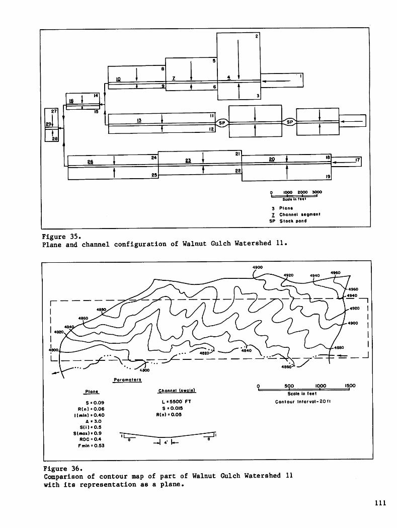
IS I "27 •5 ,

&\

28

SS

4

2

7

9

IS 18

1

« 9 6 J

3

2421

22

25t 22

SP

20 I

0 1000 2000 3000»- ' ' '

Scale In feet

3 Plane

J Channel segmentSP Stock pond

Figure 35.Plane and channel configuration of Walnut Gulch Watershed 11

19

S » 0.09

R(n)*0.06

l(mln)»0.40

A *3.0

S(i)«0.5

S(mox)»0.9

ROC = 0.4

Fmin = 0.53

L » 5500 FT

S = 0.015

R(n) =0.05

Scale in feet

Contour lntervol-20ft

-*l 4' k-

Figure 36.Comparison of contour map of part of Walnut Gulch Watershed 11with its representation as a plane.

17

Ill

112

type wgll.par

#

**********************************

*********** SYSTEM ********

**********************************

* NELE NRES NPART CLEN TFIN

29 1 0 7020. 180.#

***********************************

********* OPTIONS ***********

***********************************

NTIME NUNITS NEROS

2 10#

***********************************************




COMP. ORDER ELEMENT


DELT

3.

THETA

0.8

TEMP

-1.

(NLOG) NUM. (J)

1 1

2 2

3 3

4 4

5 5

6 6

7 7

8 8

9 9

10 10

11 11

12 12

13 13

14 14

15 15

16 16

17 17

18 18

19 19

20 20

21 21

22 22

23 23

24 24

25 25

26 26

27 27

28 28

29 29

#

Figure 37.Part of parameter file for Walnut Gulch Watershed 11

***********************************************

****** ELEMENT-WISE INFO ***

***********************************************



4 1 2 3 0 0 1 2 0 0


2840 0.0 0.015 0.50 0.50 20.0 0. 0.025 0.


9.9 4.41 0.453 .05 0.95 .01 0.12 0


*

0 0 0 0 0 0 0 0 0

*


7 0 5 6 4 0 1 1 0 0


3450 0.0 0.014 0.50 0.50 20.0 0. 0.025 0.


9.9 4.41 0.453 .05 0.95 .01 0.12 0


0 0 0 0 0 0 0 0 0

*

*

*

*

*

*

*

*

*

*


28 0 0 0 0 0 0 1 0 0


310 2260 0.148 0. 0. 0 0. 0.06 0.


0.47 4.41 0.453 0.5 0.9 0.4 0.12 0.


0 0 0 0 0 0 0 0 0

*

Figure 37--Continued.Part of parameter file for Walnut Gulch Watershed 11.

113

114

Rainfall Information

Rainfall information for an event of September 1, 1977, wasentered into the file WG11.PRE. Rainfall was measured at 10

recording raingages. The weighting factors for each plane werecalculated by dividing the total rainfall at the approximatecenter of gravity of the area corresponding to each plane by thetotal rainfall at the nearest raingage. Isohyetal maps of totalstorm rainfall were prepared to estimate the average rainfallover each plane. Weighting factors for channels are inoperativeso are shown as 9.9. Storm rainfall ranged from 0.58 in at gage55 at the upper end of the watershed to 2.35 in at gage 90 westof the watershed center. Part of the rainfall file is shown infigure 38 and .the entire file is on the enclosed diskette.

Output Files

Summary information on each plane and channel and the computedhydrograph are written to WG11.DAT, part of which is shown infigure 39. The computed and observed hydrographs from channel29 are shown in figure 40. Although some parameters have beenadjusted to provide this good fit, the parameter values areconsistent with tabulated values and also provide good fits forother events. The timing of the peaks is especially good andsuggests that the time response characteristics of the watershedhave been accurately modeled.

type wgll pre'

KINEROS Rainfall Input Data#

****************************

Gage Network Data WG11 EVENT OF 1 SEPT 77****************************

#

NUM. OF RAINGAGES MAX. NUM OF TIME-DEPTH DATA PAIRS FOR ALL GAGES

(NGAGES) (MAXND)

3110

#

There must be NELE pairs of (GAGE WEIGHT) data*

ELE. NUM. (J) PJENGAGE

4

WEIGHT

.971

2 5 .86

3 5 .97

4 1 9.9

5 1 .94

6 3 .90

7 1 9.9

8 2 1.13

9 2 1.26

10 1 9.9

11 3 .93

12 3 .95

13 1 9.9

14 2 .94

15 10 1.44

16 1 9.9

17 6 1.15

18 7 1.17

19 7 1.10

20 1 9.9

21 8 1.31

22 9 .79

23 1 9.9

24 3 .87

25 9 .93

26 1 9.9

27 10 1.09

28 10 1.11

29 1 9.9

#

*****************************

Rainfall Data*****************************


#

* ALPHA-NUMERIC GAGE ID: WALNUT GULCH GAGE #89 - GAGE NUM. 1

Figure 38.Part of rain file for event of September 1, 1977in Walnut Gulch Watershed 11.

115

116


1 27

#


# [ starting time - 1900 hrs]TIME ACCUM. DEPTH

00 0.00

29 0.03

36 0.04

39 0.08

43 0.15

45 0.19

48 0.29

51 0.50

53 0.65

55 0.76

59 0.92

62 1.02

67 1.26

74 1.49

76 1.61

79 1.75

83 1.81

103 1.83

115 1.84

119 1.86

132 1.86

139 1.87

164 1.88

169 1.92

172 1.95

184 1.96

* ALPHA-NUMERIC GAGE ID: WALNUT GULCH GAGE #51 = GAGE NUM. 2

GAGE NUM, NUM. OF DATA PAIRS (ND)

2 27f


* [ starting time - 1900 hrs]TIME

00

ACCUM. DEPTH

0.00

39 0.00

41 0.04

43 0.05

65 0.07

68 0.16

73 0.17

76 0.26

78 0.38

80 0.52

82 0.59

Figure 38—ContinuedPart of rain file for event of September 1, 1977in Walnut Gulch Watershed 11.

84 0.82

91 0.89

95 0.95

98 1.07

101 1.16

104 1.32

108 1.38

131 1.39

163 1.42

168 1.43

190 1.45

197 1.49

201 1.55

204 1.55

221 1.57

230 1.57#

* * *

* * *

* * *

* ALPHA-1

#

GAGE Nl

WJMERIC GAGE ID: WALNUT GULCH GAGE #44 = GAGE NUM. 10

JM. NUM. OF DATA PAIRS (ND)

10 27#

There must be ND pairs of time-•depth (T D) data: NOTE: The last timemust be greater than TFIN (the total computational time)

* [ starting time - 1900 hrs]TIME ACCUM. DEPTH[

00 0.00

05 0.04

08 0.08

13 0.09

32 0.12

36 0.17

39 0.24

42 0.29

47 0.42

50 0.57

52 0.71

55 0.87

58 0.99

62 1.08

66 1.13

71 1.17

95 1.21

126 1.25

131 1.34

137 1.37

152 1.40

161 1.46

169 1.52174 1.58

183 1.61

199 1.63

202 1.63*

Figure 38—ContinuedPart of rain file for event of September 1, 1977in Walnut Gulch Watershed 11.

117

00

H3

*1

no

prt

C

o i-h

o C rt

•d rt

H)

CO

O H s:

P> 8 rt

O t-1

o 3*

s:

p> rt

(D »-c

CO

^ MM

rt

zH

HZ

^P

J2

!2

!»

TJ

^!*

hd

»-a

C(D

oa

ch

CO

W»

tiO

OP

PJ

5>t-

1

to

to

to

to

to

to

to

to

to

to

»-»

1—*

1—•

1—»

1—»

1—»

1—•

1—»1

—»

1—»

f2

MW

O•

VO

OO

nJ

o>

Cn

J>

WN

3H

OV

OO

ON

lO

Mfl^w

rO

HO

vO

OO

vlO

MJi^W

MH

PJ

*>

FILE:IOMETERNFALLF

a rt

a>

n>-

aO

H3

*"Q

C5

*d

*J3

O""

dh

dtr)O

^^C

i*

Td

*d

O,T

J*

dO

^»

TJO

*T

dn

J*

d*x

JM

*J

fM

PJ

t-*

5>£>

£>5

c5>

5>5>

S>5>

^C

^S

cs>

^S

S^

Sj>

[i>

Kj>

>>

>[-•

zz

zZ

Zt^

j^»

ci^j

t?»^»

^j^

f^f^

^f^

.^^^.'

^^^'^

{'^

•g

i'^l'

^l^

l•d

PJ

II•

•P

J

2.

PJ

PI

ZP

IP

IZ

PI

PI

ZP

IP

JP

J3

PJP

JZ

PJP

JZ

PJP

J3

PJP

JZ

PJP

JP

JP

Js:

1••

PJ

PI

pj

pi

p]

PJ

PJ

PJ

PJ

I]

ff

fr"

ft*

r1f

fo I-

1P

JC

Oo

CO

o3

3ss

c\

Jtf

oo

si

i•

iI

11

11

11

II

II

<:

to

Mt-

1i-

»s

oo

oo

oo

oo

oo

oo

oo

oo

oo

oo

oo

oo

oo

oo

oP

J 1o r1

CO

hd

\H

00

M

H»I-

11-

3

hd

t^d

,-d

t-*

to

|-»

o>

to

ON

CO

4>-

«*J

o\

to

HI-'t

OvO

vl^H

HC

M-'H

UiO

O.P

'WO

NH

Nl

•P*

to

.p*

H^slO

OU

iO

H^

OH

OO

^fO

^I-1

ON

OfsU

iJi>

slW

OO

I>

^o

VO

<:

PJS

oV

O*

-JC

OO

OC

nvJvO

WH

OO

\O

HO

rO

N3

WU

lslO

WU

l0

0S

30

00

0U

vJC

y>

5*

doP

J

PJ

PJ

PJ

PI

PJ

PJ

PI

PJ

PJ

PJ

PJ

pjp

jp

jp

jp

jp

jp

jp

jp

jp

jp

jp

jp

jp

jw

pjp

jp

j3

>

'+

+>

++

++

'+

++

+«

1+

++

+'+

+'+

++

'+

'r*

2O

oO

oo

oo

oo

oo

oo

oo

oo

oo

oo

oo

oo

oo

oo

<*>

•G

MO

OtO

OO

OO

l-»

oo

l-»

oo

J|-,o

o^-1

o^-,^-,o

^-,o

oo

ro

o^-,

H M H PJ a

CO

PJ

15 C

O

o

OO

Oo

oo

oo

oo

oo

oo

oo

oo

oo

oo

oo

oo

oo

oH o

OO

Oo

oo

oo

oo

oo

oo

oo

oo

oo

oo

oo

oo

oo

oo

oo

oo

oo

oo

oo

oo

oo

oo

oo

oo

oo

oo

oo

oo

v-/

fcfo

oo

oo

oo

oo

oo

oo

oo

oo

oo

oo

oo

oo

oo

oo

>


CONTRIBUTING AREA- 72734656. SQ. FEET OR 1669.7579 ACRES


0.00 0.00000 0.000000 0.00000000 0.OOOOE+00

3.00 0.00000 0.000000 0.00000000 0.OOOOE+00

6.00 0.00000 0.000000 0.00000000 0.OOOOE+00

9.00 0.00000 0.000000 0.00000000 0.OOOOE+00

12.00 0.00000 0.000000 0.00000000 0.OOOOE+00

15.00 0.00000 0.000000 0.00000000 0.OOOOE+00

18.00 0.00000 0.000000 0.00000000 0.OOOOE+00

21.00 0.00000 0.000000 0.00000000 0.OOOOE+00

24.00 0.00000 0.000000 0.00000000 0.OOOOE+00

27.00 0.00000 0.000000 0.00000000 0.OOOOE+00

30.00 0.00000 0.000000 0.00000000 0.OOOOE+00

33.00 0.00000 0.000000 0.00000000 0.OOOOE+00

36.00 0.00000 0.000000 0.00000000 0.OOOOE+00

39.00 0.00000 0.000000 0.00000000 0.OOOOE+00

42.00 0.00000 0.000000 0.00000000 0.OOOOE+00

45.00 0.02240 0.000013 0.00000000 0.OOOOE+00

48.00 0.42309 0.000251 0.00000000 0.OOOOE+00

51.00 33.29013 0.019772 0.00000000 0.OOOOE+00

54.00 164.56206 0.097740 0.00000000 0.OOOOE+00

57.00 361.69540 0.214825 0.00000000 0.OOOOE+00

60.00 555.35382 0.329847 0.00000000 0.OOOOE+00

63.00 691.96106 0.410983 0.00000000 0.OOOOE+00

66.00 750.25299 0.445605 0.00000000 0.OOOOE+00

69.00 744.20386 0.442012 0.00000000 0.OOOOE+00

72.00 706.35266 0.419531 0.00000000 0.OOOOE+00

75.00 671.35376 0.398744 0.00000000 0.OOOOE+00

78.00 670.98926 0.398527 0.00000000 0.OOOOE+00

81.00 721.38715 0.428460 0.00000000 0.OOOOE+00

84.00 821.07404 0.487668 0.00000000 0.OOOOE+00

87.00 930.67834 0.552767 0.00000000 0.OOOOE+00

90.00 967.81537 0.574824 0.00000000 0.OOOOE+00

93.00 899.54919 0.534278 0.00000000 0.OOOOE+0096.00 772.63135 0.458896 0.00000000 0.OOOOE+00

99.00 644.59534 0.382851 0.00000000 0.OOOOE+00

102.00 543.89172 0.323039 0.00000000 0.OOOOE+00

105.00 475.31485 0.282308 0.00000000 0.OOOOE+00

108.00 428.82800 0.254698 0.00000000 0.OOOOE+00

111.00 385.60995 0.229029 0.00000000 0.OOOOE+00

114.00 332.92313 0.197736 0.00000000 0.OOOOE+00

117.00 273.42453 0.162398 0.00000000 0.OOOOE+00120.00 216.77664 0.128752 0.00000000 0.OOOOE+00

123.00 169.17757 0.100481 0.00000000 0.OOOOE+00

126.00 131.74890 0.078251 0.00000000 0.OOOOE+00

129.00 103.25227 0.061326 0.00000000 0.OOOOE+00

132.00 81.78383 0.048575 0.00000000 0.OOOOE+00

135.00 65.68036 0.039010 0.00000000 0.OOOOE+00

138.00 53.66309 0.031873 0.00000000 0.OOOOE+00

Figure 39--Continued.Part of output file for Walnut Gulch Watershed 11.

119


141.00 44.47689 0.026417 0.00000000 0.OOOOE+00

144.00 37.21624 0.022104 0.00000000 0.OOOOE+00

147.00 31.39346 0.018646 0.00000000 0.OOOOE+00

150.00 26.67612 0.015844 0.00000000 0.OOOOE+00

153.00 22.80873 0.013547 0.00000000 0.OOOOE+00

156.00 19.59949 0.011641 0.00000000 0.OOOOE+00

159.00 16.91007 0.010044 0.00000000 0.OOOOE+00

162.00 14.64006 0.008695 0.00000000 0.OOOOE+00

165.00 12.71267 0.007551 0.00000000 0.OOOOE+00

168.00 11.06776 0.006574 0.00000000 0.OOOOE+00

171.00 9.65783 0.005736 0.00000000 0.OOOOE+00

174.00 8.44509 0.005016 0.00000000 0.OOOOE+00

177.00 7.39898 0.004395 0.00000000 0.OOOOE+00

180.00 6.49444 0.003857 0.00000000 0.OOOOE+00


**** EVENT SUMMARY ***>k



BASIN AREA = 72734656. (FT**2)

TOTAL RAINFALL DEPTH - 1.542 (IN)

STORAGE REMAINING ON ALL PLANES 0.00052 (IN)STORAGE REMAINING IN CHANNELS+CONDUITS = 0.00711 (IN)STORAGE REMAINING IN PONDS = 0.00000 (IN)

TOTAL INFILTRATION FROM ALL PLANES 0.98437 (IN)TOTAL INFILTRATION FROM ALL CHANNELS 0.11664 (IN)TOTAL BASIN RUNOFF

TOTAL OF STOR., INFIL. AND RUNOF

0.43476 (IN) 2635158 0 CU.FT.

'F TERMS = 1.54339 (IN)

*** GLOBAL VOL. ERROR = 0.0811 PERCENT ***

Figure 39--Continued.Part of output file for Walnut Gulch Watershed 11

120

1000 -i

'AN900 - // \ \

in

o

800 -

700 -

600 -

////1

II

1\ \\' 1 \ls. v- / \ I

\ / \' Observed hydrograph^-^ \ \ Computed hydrograph

\\

Q>Oll_

O-COm

b

500 -

400 -

300 -

Jl

\\\\

200 -

\ \\ \\ \

100 -

\

4

' 1

0 60

i 1 i 1 i 1 i 1 i 1

80 100 120 140 160

Time (min)

Figure 40.Observed and computed hydrographsfor Walnut Gulch Watershed 11.

CONCLUDING REMARKS

The KINEROS model, implemented in FORTRAN on the encloseddiskette, simulates the response of a catchment to a user-specified rainfall event. Since runoff is generated only whenrainfall rates exceed the infiltration capacity, the modelshould not be used where other runoff-generating mechanisms areimportant. The user has an option to simulate erosion as wellas runoff, and ponds may also be included.

Since KINEROS was developed as a research tool, many options areincluded that may be of little use to the practitioner.Guidelines for estimating parameters have been presented whereinformation is available. Where there is little or no

information, runoff and erosion predictions may be subject tosignificant error if they are sensitive to the parameter inquestion.

121

122

LITERATURE CITED

Ackers, P., and W.R. White. 1973. Sediment transport: Newapproach and analysis. Journal of the Hydraulics Division,American Society of Civil Engineers 99(HY11):2041-2060.

Alonso, C.V., W.H. Neibling, and G.R. Foster. 1981. Estimatingsediment transport capacity in watershed modeling. Transactionsof the American Society of Agricultural Engineers 24(5):1211-1220, 1226.

Barnes, H.H., Jr. 1967. Roughness characteristics of naturalchannels. U.S. Geological Survey Water Supply Paper 1849, 213pp.

Bennett, J.P. 1974. Concepts of mathematical modeling ofsediment yield. Water Resources Research 10(3):485-492.

Brooks, R.H. and A.T. Corey. 1964. Hydraulic properties ofporous media. Hydrology Paper 3, 27 pp. Colorado StateUniversity, Fort Collins.

Burgy, R.H. , and CR. Pomeroy. 1958. Interception losses ingrassy vegetation. Transactions of the American Geophysical Union

Calheiros de Miranda, R.A., and D.R. Butler. 1986. Interception of rainfall in hedgerow apple orchard. Journal ofHydrology 87:245-253.

Chow, V.T. 1959. Open channel hydraulics. 680 pp. McGraw-Hill, New York.

Clark, O.R. 1940. Interception of rainfall by prairie grasses,weeds and certain crop plants. Ecological Monographs 10:243-277.

Cosby, B.J., G.M. Hornberger, R.B. Clapp, and T.R. Ginn. 1984.A statistical exploration of the relationships of soil moisturecharacteristics to the physical properties of soils. WaterResources Research 20:682-690.

Emmett, W.W. 1970. The hydraulics of overland flow onhillslopes. U.S. Geological Survey Professional Paper 662-A,68 pp.

Engelund, F. , and E. Hansen. 1967. A monograph on sedimenttransport in alluvial streams. 62 pp. Teknisk Vorlag,Copenhagen.

Engman, E.T. 1986. Roughness coefficients for routing surfacerunoff. Journal of Irrigation and Drainage Engineering,American Society of Civil Engineers 112(1):39-53.

Fair, G.M., and J.C. Geyer. 1954. Water supply and wastewaterdisposal. 973 pp. John Wiley and Sons, New York.

Foster, G.R. 1982. Modeling the erosion process. In CT.Haan, H.P. Johnson, and D.L. Brakensiek, eds., Hydrologicmodeling of small watersheds, ASAE Monograph 5, pp. 297-380,American Society of Agricultural Engineers, St. Joseph, MI.

Foster, G.R., and D.L. Meyer. 1972. Transport of soilparticles by shallow flow. Transactions of the American Societyof Agricultural Engineers 15(1):99-102.

Foster, G.R., and R.E. Smith. 1984. A dynamic erosion concept.Proceedings of the Natural Resources Modeling Symposium, PingreePark, Colo. U.S. Department of Agriculture, ARS-30, pp. 434-437.

Foster, G.R., R.E. Smith, W.G. Knisel, andT.E. Hakonson. 1983.Modeling the effectiveness of on-site sediment controls. Paper83-2092, presented at the summer 1983 meeting, American Societyof Agricultural Engineers, Bozeman, MT, 15 pp.

Glass, L.J., and E.T. Smerdon. 1967. Effect of rainfall on thevelocity profile in shallow-channel flow. Transactions of theAmerican Society of Agricultural Engineers 10(3):330-332, 336.

Goodrich, D.C, D.A. Woolhiser, and S. Sorooshian. 1988. Modelcomplexity required to maintain hydrologic response. Proceedingsof 1988 National Conference of the Hydraulic Division, AmericanSociety of Civil Engineers, Colorado Springs, CO, August 8-12,pp. 431-436.

Haynes, J.L. 1940. Ground rainfall under vegetation canopy ofcrops. Journal of the American Society Agronomy 32:176-184.

Horton, R.E. 1919. Rainfall interception. Monthly WeatherReview 47:603-623.

Julien, P.Y., and D.B. Simons. 1984. Analysis of sedimenttransport equations. Report CER83-84PYJ-DBS52, 46 pp. CivilEngineering Department, Colorado State University, Fort Collins.

Julien, P.Y., and D.B. Simons. 1985. Sediment transportcapacity of overland flow. Transactions of the American Societyof Agricultural Engineers 28(3) -.755-761.

Kibler, D.F., and D.A. Woolhiser. 1970. The kinematic cascadeas a hydrologic model. Hydrology Paper 39, 27 pp. ColoradoState University, Fort Collins.

123

124

Kilinc, M., and E.V. Richardson. 1973. Mechanics of soilerosion from overland flow generated by simulated rainfall.Hydrology Paper 63, 54 pp. Colorado State University, FortCollins.

Lane, L.J., and D.A. Woolhiser. 1977. Simplifications ofwatershed geometry affecting simulation of surface runoff.Journal of Hydrology 35:173-190.

Lane, L.J., D.A. Woolhiser, and V. Yevjevich. 1975. Influenceof simplifications in watershed geometry in simulation ofsurface runoff. Hydrology Paper 81, 50 pp. Colorado StateUniversity, Fort Collins.

Laursen, E.M. 1958. Sediment transport mechanics in stablechannel design. Transactions of the American Society of CivilEngineers 123:195-206.

Li, Ruh-Ming. 1972. Sheet flow under simulated rainfall. M.S.thesis, 111 pp., Colorado State University, Fort Collins.

Meyer, L.D., and W.H. Wischmeier. 1969. Mathematicalsimulation of the process of soil erosion by water.Transactions of the American Society of Agricultural Engineers12(6):754-762.

Morgali, J.R. 1970. Laminar and turbulent overland flowhydrographs. Journal of the Hydraulics Division, Proceedings ofthe American Society of Civil Engineers 91(HY2):441-460.

Morris, E.M., and D.A. Woolhiser. 1980. Unsteady one-dimensional flow over a plane: Partial equilibrium and recessionhydrographs. Water Resources Research 16(2):355-360.

Mutchler, C.K. , and CL. Larson. 1971. Splash amounts fromwaterdrop impact on a smooth surface. Water Resources Research7(l):195-200.

Osborn, H.B., CL. Unkrich, and D.J. Busar. 1982. Comparisonof methods to estimate runoff from small rangeland watersheds.Hydrology and Water Resources of Arizona and the Southwest,Office of Arid Land Studies, University of Arizona 12:1-8.'

Palmer, V.J. 1946. Retardance coefficients for low flow inchannels lined with vegetation. Transactions of the AmericanGeophysical Union 27(11):187-197.

Pearson, C.E., ed. 1983. Handbook of applied mathematics.1307 pp. Nostrand Reinhold Co., New York.

Podmore, T.H., and L.F. Huggins. 1980. Surface roughnesseffects on overland flow. Transactions of the American Societyof Agricultural Engineers 23(6):1434-1439, 1445.

Rawls, W.J., D.L. Brakensiek, and K.E. Saxton. 1982.Estimation of soil water properties. Transactions of theAmerican Society of Agricultural Engineers 25(5):1316-1320,1328.

Ree, W.O., F.L. Wimberly, and F.R. Crow. 1977. Manning's n andthe overland flow equation. Transactions of the AmericanSociety of Agricultural Engineers 20(l):89-95.

Rovey, E.W., and D.A. Woolhiser. 1977. Urban storm runoffmodel. Journal of the Hydraulics Division, American Society ofCivil Engineers 103(HY11):1339-1351.

Rovey, E.W., D.A. Woolhiser, and R.E. Smith. 1977. Adistributed kinematic model of upland watersheds. HydrologyPaper 93, 52 pp. Colorado State University, Fort Collins.

Schreiber, D.L. 1970. Overland flow simulation by a nonlineardistributed parameter model. Ph.D. thesis. 205 pp.Washington State University, Pullman.

Schultz, J.P., A.R. Jarret, and J.R. Hoover. 1985. Detachmentand splash of a cohesive soil by rainfall. Transactions of theAmerican Society of Agricultural Engineers 28(6):1878-1884.

Smith, R.E. 1978. Simulating erosion dynamics with adeterministic distributed watershed model. In Proceedings ofthe Third Inter-Agency Sedimentation Conference, pp. 1.163-1.173, Sedimentation Committee, Water Resources Council,Washington, D.C

Smith, R.E. 1981. A kinematic model for surface mine sedimentyield. Transactions of the American Society of AgriculturalEngineers 24(6):1508-1514.

Smith, R.E. 1983. Flux infiltration theory for use inwatershed hydrology. In Proceedings of the National Conferenceon Advances in Infiltration, pp. 313-323, American Society ofAgricultural Engineers, St. Joseph, MI.

Smith, R.E., D.L. Chery, K.G. Renard, and W.R. Gwinn. 1982.Super-critical flow flumes for measuring sediment-laden flow.U.S. Department of Agriculture Technical Bulletin 1655, 70 pp.

Smith, R.E., andJ.-Y. Parlange. 1978. A parameter-efficienthydrologic infiltration model. Water Resources Research14(3):533-538.

125

126

Tromble, J.M. 1983. Interception of rainfall by tarbush.Journal of Range Management 36:525-526.

U.S. Department of Agriculture. 1975. Soil taxonomy. U.S.Department of Agriculture Handbook 436, 752 pp.

Unkrich, C.L., and H.B. Osborn. 1987. Apparent abstractionrates in ephemeral stream channels. Hydrology and WaterResources in Arizona and the Southwest, Offices of Arid LandStudies, University of Arizona, Tucson, 17:34-41.

Wheater, H.S., and N.C. Bell. 1983. Northern Oman flood study.Proceedings Institution of Civil Engineers, part 2, 75:453-473.

Wischmeier, W.H., and D.D. Smith. 1965. Predicting rainfallerosion losses from cropland east of the Rocky Mountains. U.S.Department of Agriculture Handbook 282, 47 pp.

Wischmeier, W.H., and D.D. Smith. 1978. Predicting rainfallerosion losses--a guide to conservation planning. U.S.Department of Agriculture Handbook 537, 58 pp.

Wisheropp, P.L. 1982. Identification of the storm infiltrationpattern using kinematic back-routing. M.S. thesis. 116 pp.Civil Engineering Department, Colorado State University, FortCollins.

Wooding, R.A. 1965. A hydraulic model for the catchment -stream problem. I. Kinematic wave theory. Journal ofHydrology 3(3):254-267.

Woolhiser, D.A. 1975. Simulation of unsteady overland flow.In K. Mahmood and V. Yevjevich, eds. , Unsteady Flow in OpenChannels, v. II, p. 502, Water Resources Publications, FortCollins.

Woolhiser, D.A., CL. Hanson, and A.R. Kuhlman. 1970. Overlandflow on rangeland watersheds. Journal of Hydrology (NewZealand) 9(2):336-356.

Woolhiser, D.A., and J.A. Liggett. 1967. Unsteady, one-dimensional flow over a plane--the rising hydrograph. WaterResources Research 3(3):753-771.

Wu, Y-H, V. Yevjevich, and D.A. Woolhiser. 1978. Effect ofsurface roughness and its spatial distribution on runoffhydrographs. Hydrology Paper 96, 47 pp. Colorado StateUniversity, Fort Collins.

Yalin, Y.S. 1963. An expression for bed-load transportation.Journal of the Hydraulics Division, Proceedings of the AmericanSociety of Civil Engineers 89(HY3):221-250.

Yang, CT. 1973. Incipient motion and sediment transport.Journal of the Hydraulics Division, American Society of CivilEngineers 99(HY10):1679-1704.

Yu, Y.S., and J.S. McNown. 1964. Runoff from impervioussurfaces. Journal of Hydraulic Research 2(1):3-24.

127

128

APPENDIX: SEDIMENT TRANSPORT CAPACITY RELATIONS

AVAILABLE IN KINEROS

The following transport capacity relations are numbered as intable 10 and as inputted under LAW in the parameter input file.Each expression defines an "equilibrium" sediment concentrationin terms of hydraulic and sediment parameters.

Most of the symbols used are defined under "Symbols;" others aredefined as they appear in this section.

u^ -JghdS [L/T]

hd = hydraulic depth, flow area divided by top width [L]

p = particle density [m/L ]

1. Simple tractive force (Meyer and Wischmeier 1969)

4

C = C -mx s

u

[A.l]

2. Unit stream power (Yang 1973) (only for 0.062mm < d < 2mm)

loSin^eCmv) = "°-565 - 0.286A - 0.457B + C D [A.2iu s mx p P P P

v ds

in which A = log. _p &10

and

with

where

log (u^/v )

C = 1.799-0.409A -0.314BP P P

Dp "loS10[<u/vs "VS]

, (ioglnET,2:5o.o6)+ °'66' °<Ep<70

*

10 p

or 2.05; E >70P

3. Bagnold/Kilinc (Kilinc and Richardson 1973)

1.67

; t > tmx

"oh* - fc)]h7 u

w

in which r = 7 hS.w

7 = specific weight of water,

r = shields critical tractive force, andc '

C = parameter

4. Ackers and White (1973) (only for d > 0.04 mm)

dC

mx h

in which

u,n

-in

u

u,

F =g

Ki*.-1)

F-S

AP

m

(io6)

u

J32 log1()(10h/d)

1-n

and in which, defining dimensionless grain diameter as

nV3g(ss-i)d = d

g

the following parameter definitions apply:

'1-0.56d ; 1 < d < 60g g

n = "

lo; d > 60g

r0.23/Jd + 0.14; 1 < d < 60g g

,0.170; d > 60g

r9.66/d + 1.34; 1 < d < 60g gm = «

[1.50; d > 60g

[A.3]

[A.4]

[A.5]

>.6]

[A.7]

[A.s;

[A.9]

129

130

and

[log(dg)]log C =2.86 log d - log(d ) - 3.53; 1 < d < 60 [A.10]r o L o J o

or

C = 0.025; d > 60P g

5. Yalin (1963):

C = 0.635duAS ~zmx * s uh

in which

1-J—"lnfl+A B1B A I n pip n v trj

A - — - 1 ; Y > Yn Y ' c

c

= 0 otherwise

B _ 2,45 I

s

u,

(Sg-l)gd

[A.11]

[A.12]

Yc = critical tractive force, based on particle Reynoldsnumber

6. Engelund and Hansen (1967):

0.05 u u.3

™ g2dh(ss-i)2 [A.13]

* U.S. GOVERNMENT PRINTING OFFICE: 1990—720-599/D6639

Documentation and User Manual - Southwest … Kinematic Runoff and Erosion Model: Documentation and...

Documents

Transcript of Documentation and User Manual - Southwest … Kinematic Runoff and Erosion Model: Documentation and...