DOCUMENT RESUME ED 236 301 UD 023 191 … · AUTHOR Farkas, George; And Others ... Valuable...

DOCUMENT RESUME

ED 236 301 UD 023 191

AUTHOR Farkas, George; And OthersTITLE Impacts from the Youth Incentive Entitlement Pilot

Projects: Participation, Work, and Schooling Over theFull Program Period.

INSTITUTION Manpower Demonstration Research Corp., New York,N.Y.

SPONS AGENCY Employment and Training Administration (DOL),Washington, D.C. Office of Youth Programs.;Employment of Training Administration (DOL),Washington, D.C; Office of Research andDevelopment.

PUB DATE Dec 82GRANT 28-36-78-36NOTE 328p.PUB TYPE Reports - Evaluative/Feasibility (142)

EDRS PRICE MF01 Plus Postage. PC Not Available from EDRS.DESCRIPTORS Black Employment; *Demonstration Programs;

Disadvantaged Youth; *Dropout Prevention;Economically Disadvantaged; *Education WorkRelationship; High School Graduates; High SchoolStudents; Hispanic Americans; Job Development; *LowIncome Groups; Out of School Youth; ProgramEffectiveness; Program Evaluation; Reentry Students;Secondary Education; *Student Employment; *WelfareRecipients; Youth Employment

IDENTIFIERS *Youth Entitlement Incentive Pilot Projects

ABSTRACTThe Youth Incentive Entitlement Pilot Projects

(YIEPP) demonstration, which was in full operation from 1978 to 1980,was established to test the efficacy of work combined with educationas a remedy for high unemployment, low labor force participation, andthe'excessive school dropout rate of teenagers. YIEPP offered Federalminimum-wage jobs (part-time during the school year, full-time duringthe summer) to 16- to 19-year-olds from low-income or welfarehouseholds, with the condition that they complete their high schooleducation, either through traditional or alternative educationprograms. Analysis of the impact of the demonstration found that (1)over 56 percent of the eligible youths participated in YIEPP at leastonce; (2) YIEPP increased the employment/population ratio foreligible youth by 67.5 percent over the ratio expected-in the absenceof the program; (3) YIEPP was particularly successful with blackYouth, whose employment, increased by 102.8 percent, became nearlyequal to the employment percentages of white male youth; and (4) thesmallest statistically significant YIEPP effect was found forHispanic females, and there were no significant effects for Hispanicmales. Additional effects were that total school enrollment increasedsignificantly, the dropout rate decreased, and the rate of return toschool (whether in traditional or alternative programs) forout-of-school youth increased. Finally, YIEPP caused a positive jointincrease in schooling and work behavior among the key groups ofprogram youth. (CMG)

Manpower'Demonstration

ResearchCorpOration

IMPACTS FROM THEYOUTH INCENTIVE

ENTITLEMENTPILOT PROJECTS

PARTICIPATION,WORK, ANDSCHOOLING

OVER THE FULL-PROGRAM PERIOD

"PERMISSION TO REPRODUCE THISMATERIAL IN MICROFICHE ONLYHAS BEEN GRANTED BY

KATFI-AYN goi3IPSonb2,tAkire74-trai

ge5cLiNr Car {IsTO THE EDUCATIONAL RESOURCESINFORMATION CENTER (ERIC)."

U.S. DEPARTMENT OF EDUCATIONNAT NAL INSTITUTE OF EDUCATION

EDU ATIONAL RESOURCES INFORMATIONCENTER (ERIC)

This document has been reproduced asreceived from the person or organizationoriginating it.

O Minor changes have been made to improvereproduction quality.

Points of view or opinions stated in this dorm-ment do not necessarily represent officialNIEPOsitOrt or poky.

(;eoi-gc1). AltonErnst \V.(;ail TrasRobertAWL- AS,'

Deceni

BOARD OF DIRECTORSRICHARD P. NATHAN, ChairmanProfessorWoodrow Wi 'SOH School of .

Public and International AffairsPrinceton University

M. CARL HOLMAN, Vice-ChairmanPresidentNational Urban Coalition

PAUL H. O'NEILL, TreasurerSenior Vice-PresidentInternational Paper Company

ELI GINZBERG, Chairman EmeritusDirectorConservation of Human ResourcesColumbia University

BERNARD E. ANDERSON.DirectorSocial Sciences DiVisionRockefeller Foundation

JOSE A. CARDENASDirectorIntercultural Development Association

ALAN KISTLERDirector of Organization and Field ServicesAFL-CIO

RUDOLPH G. PENNERResident ScholarAmerican Enterprise Institute for

Public Policy Research

DAVID SCHULTEVice-PresidentSalomon Brothers

ROBERT SOLOWInstitute ProfessorMassachusetts Institute of Technology

GILBERT STEINERSenior FellowBrookings Institution

PHYLLIS A. WALLACEProfessor

.Alfred P. Sloan School of ManagementMassachusetts Institute of Technology

NAN WATERMANTreasurer, Board of DirectorsChildren 'sDefense Fund

EXECUTIVE STAFFBARBARA B. BLUM, President

JUDITH M. GUERON, Executive Vice-President

GARY WALKER, Senior Vice-President

ROBERT C. PENN, Vice-President

MICHAEL R. BANGSER, Vice-President

3

Manpower Demonstration Research Corporation

IMPACTS FROM THE YOUTH INCENTIVE ENTITLEMENT PILOT PROJECTS:

PARTICIPATION, WORK, AND SCHOOLING OVER THE FULL PROGRAM PERIOD

George FarkasD. Alton SmithErnst W. StromsdorferGail TraskRobert Jerrett, III

Abt Associates Inc.

Prepared for:

Manpower DemonstrationResearch Corporation

December 1982

This report was prepared pursuant to the Youth Employment andDemonstration Project Act of 1977 (PL-95-93), Title II, "Youth IncentiveEntitlement Pilot Projects."

Funding for this national demonstration was provided by the Officeof Youth Programs of the Employment and Training Administration, the U.S.Department of Labor, under Grant No. 28-36-78-36 from the Office ofResearch and Development of ETA.

Researchers undertaking such projects under government sponsorshipare encouraged to express their professional judgments. Therefore,

points of view or opinions stated in this document do not necessarilyrepresent the official position or policy of the federal governmentsponsors of the demonstration.

Copyright 1982 by the Manpower Demonstration Research Corporation

ACKNOWLEDGEMENTS

The author for the Executive Summary and Chapter 1 was Ernst W.

Stromsdorfer. Robert Jerrett wrote Chapter 2. The analysis for Chapters

3 through 6 was designed by George Farkas and D. Alton Smith, in con-

sultation with Messrs. Stromsdorfer and Randall J. Olsen. Data manage-

ment, variable creation, and associated computer and statistical work was

performed by Gail Trask, who was assisted by Jane Kulik and Linda Sharpe.

Computations in Chapters 3 and 4 were carried out by D. Alton*Smith, who

also wrote these chapters in association with George Farkas. Computa-

tions in Chapter 5 were carried out by Trask and by Smith in Chapter 6,

while both chapters were written by Farkas. All material was edited by

Ernst Stromsdorfer and Felicity Skidmore. Annette Butler produced the

report.

Valuable technical criticism and editorial advice were provided by

Judith Gueron, Robert Cook, and Sheila Mandel of the Manpower Demonstra-

tion Research Corpration and Alan L. Gustman of Dartmouth College.

YIEPP SITES AND CETA PRIME-SPONSORS

Tier I

Site Prime Sponsor

Baltimore, Maryland Mayor's Office of Manpower Resources

Boston, Massachusetts Employment and Economic PolicyAdministration

Cincinnati, Ohio City of Cincinnati Employment andTraining Division

Denver, Colorado Denver Employment and TrainingAdministration

Detroit, Michigan

King County, Washington

Southern Rural Mississippi

Tier II

Alachua County, Florida

Albuquerque, New Mexico

Berkeley, California

Employment and Training Department

The King County Consortium

Governor's Office of Job Developmentand Training

Alachua County CETA

City of Albuquerque Office of CETA

Office of Employment and CommunityPrograms

Dayton, Ohio Office of the City ManagerManpower Planning and Management

Monterey County, California Monterey CETA Administration

Nashua County, New Hampshire Southern New Hampshire Services/CETA

New York, New York Department of Employment of theCity of New York

Philadelphia, Pennsylvania City of Philadelphia AreaManpower Planning Council

Steuben County, New York Steuben County Manpower Administration

Syracuse, New York City of Syracuse Office of Federaland State Aid Coordination

-iv-

PREFACE

A number of studies have documented the employment problems faced

by low-income, often minority, youths who are growing up with minimal

exposure to the work world. Many of these same youths have either

dropped *ot of school or are at risk of doing so. These patterns

threaten to severely undermine their aspirations for a positive work

future.

Although the past decade has witnessed a number of efforts designed

to help these youths find a place in the labor market, there have been

some important gaps in the nation's overall approach to this problem.

First, many such programs gave young people jobs, but failed to address

their schooling; there was even the danger that, rather than reinforce

their learning experience, some programs would draw youths away from

school. Another consequence, too, was that the two institutions most

intimately involved with the improvement of skills among young people --

the employment and training system and the schools -- were often given

little reason to work together. Finally, these programs were usually not

implemented on a scale sufficient to have a major impact on the youths'

opportunities.

The Youth Incentive Entitlement Pilot Projects (YIEPP) provided en

unusual occasion to learn about the feasibility and outcomes of a large,

coherently defined program designed to link schooling and work. The

MDRC is publishing simultaneously the full impact and implementation

findings on the operational period of the Youth Incentive EntitlementPilot Projects demonstration. This preface introduces both this impact

report and its companion volume, Linking School and Work for Disad-vantaged Youths: The YIEPP Demonstration: Final Implementation Report.

-v-

YIEPP demonstration introduc0two major innovations: the program model

itself -- where 16- to 19-year-old disadvantaged youths were offered a

part-time job during the school year and a full-time job in the summer on

the condition that they stay in school and meet academic and job-related

performance standards -- and the scale of implementation, where the job

offer was extended to all eligible youths in 17 designated demonstration

areas. Over 76,000 youths joined and were given jobs during the full;

demonstration period.

In 1977, the Department of Labor's Office of Youth Programs contract-

ed with the Manpower Demonstration Research Corporation (MDRC) to conduct

the research and oversee the operations of the YIEPP demonstration.

Based on an agenda identified in the:1977 Youth Act, a large, four-part

research program was designed to address: (1) the number of youths to

participate from among those eligible and the program's short- and longer-

run impacts on employment and schooling behavior; (2) the feasibility of

the program model and other operational lessons; (3) the cost of the

demonstration and its replication or expansion; and (4) a number of

special issues, including the quality of work provided to the youths and

the significant role of businesses in an unprecedented private sector job

creation effort.

Reports issued to date have covered the initial period of program

implementation, early impacts, and many special issues. The two reports

published at this time summarize the implementation and impact lessons

from the full 30-month demonstration period and provide cost data. A

final report scheduled for 1983 will examine whether YIEPP had longer-

term, poSt-program effects on the youths' educational and employment

behavior.

The two current volumes contain significant findings about the YIEPP

approach. Somewhat surprisingly, the implementation report indicates

that the prime sponsors did not encounter major problems in meeting the

difficult challenges of delivering on a job" guarantee. What proved more

troublesome was the enforcement of the school performance conditions,

responsibility shared with the school systems involved. However, despise

start-up difficulties, the report suggests that the demonstration's

overall record was one of significant managerial achievement.

Perhaps the most compelling part of the program's record, as seen in

both of these reports, is its success in attracting black youths: they

are seen joining YIEPP in greater numbers and staying in it longer than

any other group. This finding is particularly significant in the context

of the experience of the past 25 years, when there has been a consistent

and dramatic decline in minority youth employment, particularly for

males. Thus, while in 1955 black male youths were employed at the same

rate as whites, by 1981 their employment rate had been cut in half, while

that of white youths remained constant or improved. A similar, though

somewhat less dramatic, 'story holds true for young minority women.

While these facts are clear, the explanation is not. Before the

YIEPP demonstration, there had been relatively little evidence to help in

sorting among the conflicting explanations of job shortages, discrimina-

tion, lack of motivation, unrealistic wage expectations, or the attrac-

tion of more profitable extra-legal alternatives. .YIEPP, with its job

guarantee, provided a unique, direct mechanism to test youths' interest

10

in working. The striking finding in the impact study, where YIEPP is

seen to double minority youths' school-year employment rates -- bringing

them essentially equal to or exceeding those for white youths -- suggests

that the prevailing low employment rate is not voluntary. YIEPP's'

impacts on school enrollment, while more modest, are also positive.

While the program did not reverse declining enrollment as youths' pro-

gressed through high school, it slowed this down, through both reducing

the drop-out rate and increasing the numbers of youths returning to

school.

From the varied lessons in both reports, YIEPP emerges as a program-

matic intervention that encourages school completion and the compilation

of a work-history. Moreover, the program proved feasible to implement on

an extremely large scale. The management record of the YIEPP prime

sponsors is testament to the fact that large numbers of jobs can be

developed to alleviate youth unemployment, and that these jobs can

provide a meaningful work experience. Perhaps, most of all, YIEPP has

shown that, when jobs are available, young people do want to work -- even

at the minimum wage, and even while still continuing in school.

While a job guarantee as a solution to large-scale labor market

weaknesses may not seem currently affordable, the lessons on the YIEPP

model itself are of pointed relevance. The guarantee itself was not

essential to the rest of the program model. YIEPP cccld be operated as a

slot program while still retaining its other featur.3; in fact, this

occurred in a transition year immediately following to demonstration

period. Much of the YIEPP experience should be of inter st in view of

the new Job Training Partnership Act, which reflects te country's

tt

viii-11

continued focus on preparing youths for employment and on models that

link school and work, demanding performance from the youths in exchange

for a job. In'short, these two reports provide many lessons that future

planners of youth programs will find instructive.

Judith M. GueronExecutive VicePresident

Manpower DemonstrationResearch Corporation

Table of Contents

Page No.

xvii

1

1

7

12

15

17

17

22

24

32

40

42

45

47

47

4749

61

67

71

71

75

83

90

98

Overview

CHAPTER 1 THE PROGRAM AND ITS NATIONAL POLICY CONTEXT

The Policy Problem- The Features and Goals of the Youth Incentive

Entitlement ProjectImplementation FactorsPlan of the Study: Exepcted Effects of YIEPPduring the Program Period.

CHAPTER 2 RESEARCH DESIGN AND SAMPLE ISSUES

Research Design- The Longitudinal Survey

Analysis SamplePilot and Comparison SitesAttrition from the Baseline Longitudinal SampleProgram EligiblesSummary

CHAPTER 3 PROGRAM PARTICIPATION

- IntroductionMeasuring Program ParticipationProgram Participation RatesParticipant Program Experiences and the Durationof Program ParticipationSummary

CHAPTER 4 PROGRAM EFFECTS ON SCHOOL ENROLLMENT

- Measurement IssuesProgram Effects onof Degree ProgramProgram Effects on15- to 16-year-oldProgram Effects onRace and SexSummary

School.

SchoolCohortSchool

Enrollment by Type

Enrollment for the

Enrollment by Site,

Table of Contents(Continued)

Paae No.

CHAPTER 5 PROGRAM EFFECTS ON EMPLOYMENT AND LABORFORCE PARTICIPATION 101

- The Context of the Analysis 101

- Program Effects on the Employment/Population Ratio 108

- Net Job Creation 123

- Program Effects on Labor Force Participation,Employment, and Unemployment Rates 127

- Program Effects for the 15- to 16-year-old Cohort 131

- Employment/Population Ratios and Wage Ratesfor Employed Youths 134

- Comparison with United States Average Employmentand Unemployment Statistics 135

- Summary 137

CHAPTER 6 PROGRAM EFFECTS ON SCHOOL ENROLLMENT AND EMPLOYMENT,JOINTLY CONSIDERED 139

- Total Program Effects- Program Effects by Primary School and Work

Status in the Preprogram Period- Summary

140

142146

APPENDIX A Supplementary Impact Tables 151

APPENDIX B Regression Models for Basic Program Impacts 173

APPENDIX C Tests of Sample Attrition Bias 241

14

List of Tables

TABLE Page No.

1 . 1 Percent of High school Dropouts among Persons 16 to19 Years Old, by Age, Race and Sex: United States,October, 1977, 1978 and 1979 3

1.2 Number of Youths Assigned in YIEPP Projects 12

2.1 Number of Youths Working in YIEPP Jobs 21

2.2 Characteristics of the Analysis ilample at Baseline 25

2.3 Marital and Parental Status of the Analysis Sampleover Time 30

2.4 The YIEPP Sample Compared with the National LongitudinalSurvey of'Young American Samples* 31

2.5 YIEPP Evaluation Sites Compared to YIEPP Total andthe Nation 34

2.6 Selected Characteristics of the Pilot and ComparisonSites 36

2.7 Analysis Sample Characteristics of Pilot and ComparisonSites 38

2.8 Characteristics of Baseline Longitudinal and AnalysisSamples 41

2.9 Program Eligibles, Spring 1978 - Summer 1980 44

3.1 Program Participation Rates by Site and Period 50

3.2 Program Participation Rates by Cohort and Period... 53

3.3 Program Participatioh Rates (Spring 1978 - Summer 1980)by Cohort, Race and Sex 55

3.4 Adjusted Program Participation Rates 57

3.5 Program Participation Rates by Sex, Family Statusand Period 58

3.6 Program Participation Rates by School and Work Statusin the Previous Period 60

3.7 Participant Program Experience by Site 62

List of Tables(Continued)

TABLE Page No.

3.8 Duration of Program Participation' by Site, forProgram Participants 65

3.9 Duration of Program Participation by Cohort, Race and66Sex, for Program Participants

3.10 Adjusted Duration of Program Participation by Site,Cohort, Race and Sex, for Program Participants 68

4.1 School Enrollment Rates by Type of Degree Program .

and Pilot or Control Sites 76

4.2 Program Effects on School Enrollment Rates by Type'of Degree Program 78

4.3 Program Effects on Dropout and Return-to-School Rates 80

4.4 Enrollment Characteristics by Pilot or Control Site 84

4.5 Program Effects on Enrollment, Dropout and Return-to-School Rates for the 15- to 16-year-old Cohort 86

4.6 Cumulative Pz.vgram Effects on School Enrollment Ratesfor the 15- to 16-year-old Cohort 88

4.7 Program Effects on Total School Enrollment RatesBy Site 91

4.8 Program Effects on Enrollment, Dropout and Return-to-School Rates by Race 93

4.9f Program Effects on Enrollment, Dropout and Return-to-r School Rates by Sex 96

5.1 Total Unemployment Rates (Individuals of All Ages) inPilot and Control Sites: Annual Averages, 1975-1980.... 103

5.2 Average EMployment/Population Ratios, by Pilot orControl Site, and Period 109

0

5.3 Program Effects on Employment/population Ratios,Full Study Sample 110

5.4 Program Effects on Employment /population Ratios forthe 15- to 16-year-old Cohort, Separately by Period 113

5.5 Program Effects on Employment/population Ratios,Separately by Site 115

TABLE

5.6

5.7

5.8

5.9

List of Tables(Continued)

Program Effects on Employment/Population Ratios,Separately by Sector

Program Effects on Employment/Population RatiosSeparately by Period, Sex, and Race

Page No.

117

120

Net Job Creation, by Season and Period 125

Average Labor Force Participation, Employment, andUnemployment Rates, by Pilot or Control Site andPeriod

5.10 Program Effects on Labor Forceand Unemployment Rates

Participation, Employment,

5.11 Program Effects on Labor Forceand Unemployment Rates for theSeparately by Period

128

129

Participation, Employment,15- to 16-year-old Cohort,

132

5.12 Employment/Population and Unemployment/PopulationRatios for 16- to 19-year-old youths by Race and Sex:YIEPP Sample and United States Averages for October1978 136

6.1 Program Effects on the Percentage of Program-EligibleTime Spent in Different School and Employment States.... 141

6.2 Program Effects on the Percentage of Program-EligibleTime Spent in Different School and Employment States,by Primary State in the Preprogram Period 143

List of Figures

FIGURES Page No.

1.1 Employment/Population Ratios by DemographicCharacteristics, 1955-80 4

1.2 Civilian Labor Force Participation Rate by DemographicCharacteristic, 1955-80 5

1.3 Unemployment Rates by Demographic Characteristics,1955-80 6

5.1 The Mechanism of Program Effect on Total Employment forthe Target Population 106

18-xvi-

OVERVIEW

INTRODUCTION

The Youth Incentive Entitlement Pilot Projects (YIEPP) demonstration

was established to test the efficacy of work combined with education as a

remedy to high unemployment, low labor force participation, and the

excessive school dropout rates of teenagers. The demonstration began in

the spring of 1978, and the period of full operations. -- the focus of

this report -- extended through August of 1980.

Description of the Program

The YIEPP program 'wag-targeted to youths aged 16 to 19, from law-

income-or-welfare-householdsr-who had Triot-yet -grSduated from high school.

Its primary feature was an offer of a guaranteed, federal minimum wage

job, part-time during the school year and full-time during the summer, on

condition that youths remain in or return to school or pursue a General

Equivalency Diploma (GED) through an alternative educational program.

For YIEPP participants, getting and keeping this subsidized job was

conditional on satisfactory schooling and job performance.

An important difference between this and previous programs intended

to draw youths back to school was that both school and work performance

standards were to be met as a condition of remaining' in the program. The

schooling requirement eliminated the possibility that some youths

would quit school to take advantage of a subsidized job -- a potential

problem in other subsidized employment programs and strategies (such as a

youth subminimum wage) designed to increase employment for this popula-

tion.

19

The program was based on the empirically suggested premise that

youths who are both in the labor market and attending school fare better

in terms of earnings and employment after leaving school than those who

drop out of either school or the labor market. In particular, youths who,

are neither in the labor market nor in school appear to suffer long-term

economic disabilities. While such youths are a prime target for this

program, YIEPP concentrated as well on

in-school population.

The short rungoals of YIEPP were to:

Reduce the school dropout rate

Increase the high school graduation rate

Provide work experience

Provide income

The long-run goal was to increase labor productivity and thereby improve

life-cycle employability and earnings. In addition, participants might

acquire additional postvecondary education.

These goals were to be accomplished through the

providing work experience for an

improved performance in school and a meaningful work

participants'

experience. The

operational objectives of the demonstration were to document the poten-

tial demand for the program by youths and employers

its administrative feasibility.

The Social Problem

The social problem addressed by YIEPP is chronic

This joblessness has developed and worsened over

and to demonstrate

yOuth joblessness.,

the past several

decides, particularly'among black youths, who represent the tine of the

problem.

20

The evidence is striking. During the past 25 years, the employment/

population ratiol for white teenage males (aged 16 to 19) has remained

at about 90 percent of that for all workers. In contrast, the employ-

ment/population ratio for black male teenagers, which was comparable to

that for white teenage males in 1954, has declined by about 50 percent in

the last 15 years, even falling below that of white teenage females in

1968. For black teenage females -- the group with the worst experience

of all -- the employment/population ratio dropped in 25 years from 48 to

39 percent of that for all workers. The story is similar for labor force

participation and unemployment rates.

School dropout statistics are equally discouraging. While dropout

rates at ages 16 and 17 are similar for.blacks and whites, both male and

female, by ages 18 and 19 black males and females experience dropout

rates ranging as much as 37 to 58 percent higher than 18- and 19-year-old

comparable white youths over the 1977 to 1979 time period. Hispanic

youth dropout rates are even worse when compared to rates: for white

youths.

The potential causes for these phenomena are multiple and inter-

acting. First, much of the high level of unemployment (looking for but

unable to find a job) and ncnemployment (not looking for a job), regard-

less of sex and race, is attributable to normal life cycle patterns of

work activity for this age group. Business cycle adjustments also

fall disproportionately on new labor force entrants and persons with

1The employment/population ratio is the number of employed indivi-

duals in a given group divided by the total number of individuals in thatgroup.

21

short job tenure. Second, the geographic distribution of employment

demand is a contributing factor, exaceilated by the movement of jobs from --

the central city. Finally, the minimum wage requirement may play a

negative role in the hiring of entry-level young unskilled workers (Wise

and Meyer (1982)).

However, these factors alone cannot explain youth joblessness.

For example, the' employment situation for white female teenagers has

improved dramatically despite relatively depressed economic growth over

the past decade. Factors that go beyond the characteristics and condi-

tions that affect available jobs (the demand side of employment) and deal

with the special characteristics of the teenager labor force (the supply

side of employment) are also at work. Yet while these factors are

explored below, it is important to note that the demand and supply

conditions operate jointly to account for the joblessness problem.

Among the significant supply side factors is an increase in the

population size of young persons which has led to more competition

for jobs and, in addition, depressed their wage rates in comparison

to adults. Ironically, the similarity of wage rates for this age group

may work against blacks to the. extent that some employers may discri-

minate racially in their hiring in favor of white youths.

A second set of factors involves inadequate education, skills

and motivation levels of youths, as well as broad socioeconomic problems

associated with inner-city life. The specification and measurement

of these factors are difficult but it is clear that drug and alcohol

abuse, youth crime, broken homes, high teenage pregnancy rates, and poor

schooling and work habits contribute in the aggregate to youth jobless-

ness. The increased level of welfare payments, which may lower the

incentive to work at current wage rates, is seen as another contributing

factor.

The YIEPP policy response to both demand and supply side factors

is a joint strategy: it deals with the demand side problem of job avail-

ability by directly providing jobs; it deals with the structural and

supply side problem by enhancing educational and job-related skills.

The Potential Significance of YIEPP

The YIEPP demonstration, among all the programs and demonstrations

fostered by the Youth Employment and Demonstration Projects Act of 1977

(with the possible exception of the Job Corps), offered the most coherent

and focused attack on the joint problems of youth joblessness and school

dropout behavior.

Analyses of previous youth employment and training programs suggest

the following lessons in policy and design (Stromsdorfer 1980):

Work experience alone may not improve the long-run employa-bility or school attendance of youths, especially if the jobsare ill-defined, with low-quality supervision.

Work experience may be more effective when it is combined withother services such as job placement, skills training, or basiceducation.

Though poorly tested, services aimed at changing personalitytraits and personal values have not yet been shown to besuccessful. Of all the services offered to youths other thanskills training and work experience, job placement servicesappear to be the most effective.

Success in the workplace is directly related to basic writing,communication, and computational skills.

Successful program administration requires the development andmaintenance of minimum behavioral and program performancestandards. Effective management is a necessary condition foran effective program.

In response to these lessons, the YIEPP demonstration incorporated the

following positive features:

A job at the federal minimum wage was provided to all eligibleyouths who wanted one.

While the program itself only provided employment, work experi-ence and schooling (or participation in a GED program) werejoint requirements for participation; one could not occurwithout the other.

Work and school performance standards were established, and

efforts were made by program managers to enforce them.

The emphasis on return to, and completion of, schooling (oracquiring a GED) implied an emphasis on basic language andcomputational skills.

Services were directed mainly toward the successful completionof school and a meaningful work experience.

The quality of program management was relatively high, inpart, because of an extensive third-party monitoring.

This combination of features created a relatively straightforward and

coherent program model. The "treatment" provided was explicit; it

attempted to combine work and school experiences for youths in a comple-

mentary and mutually reinforcing way.

RESEARCH DESIGN

The research design underlying the impact analysis had two major

characteristics. First, it made use of matched comparison sites, chosen

to help measure net program effects. Second, it focused on program

eligibles, not just participants.

Comparison sites. The matched pairs on which the evaluation was

based were:

Pilot Site

Denver, ColoradoCincinnati, OhioBaltimore, MarylandMississippi'(eight rural counties)

Comparison Site

Phoenix, ArizonaLouisville, KentuckyCleveland, OhioMississippi(six rural; counties)

These eight sites were paired on the basis of similar economic and

demographic characteristics, and in each one, a random sample of program-

eligible youths was identified. The study sample of youths eligible for

YIEPP in June, 1978 shortly after its inception was weighted heavily (over

35 percent) toward youths aged 15 And 16. This strateg,i7.-allowed a large

portion of the youths to age into eligibility during the demonstration

and attain the maximum potential period of exposure to the program. The

behavior of youths in this cohort would thus approximate the experience

of an ongoing program.

A series of four questionnaires was administered to the sample,

covering the youths' schooling, work, and related experiences. The first

examined their preprogram period behavior, the second and third, the

period during program operations, and the fourth, their post-program

experiences. This document is based on an analysis of the first three

waves of interviews, and thus uses longitudinal data from January, 1977

through the fall of 1980.

The data indicate that the sociodemographic characteristics of pilot

and comparison site youths, while not perfectly matched, were quite

similar. Multiple regression analysis was used to adjust for residual

differences .across sites, but the.four pilot sites still must be re-,

garded as four distinct experiments in program administration. This

impact evaluation therefore considers each pilot site or pilot/Comparison

pair on its own terms as revealing what happens when a program such as

YIEPP is introduced into a particular environment. Four-site and three-

site aggregations (the latter exclude the Denver-Phoenix pairtfor reasons

discussed below) are used to express average program impacts.

The Focus on Eligibles. In an entitlement program, it is not

possible to assign youths randomly to program and nonprogram groups and

to systematically deny YIEPP services to the latter group. The alterna-

tive strategy chosen, therefore, used comparison communities, as noted

above, and program-eligible youths in both pilot and comparison sites.

While this approach risks the possibility of attributing effects to the

program that really result from differences among communities, it has a

key advantage in that it can, ignore competition for jobs in the pilot

site between participants and nonparticipants an important fact in a

program where participants are entitled to a j. guarantee.

One additional policy reason for foci. S. on eligibles was the

Congressional mandate to measure program take-L,p rates, the composi-

tion of program participation, and the factors that influenced partici-

pation.

PROGRAM IMPLEMENTATION AND OPERATIONS

The program and research has been coordinated throughout by the

Manpower Demonstration Research Corporation (MDRC), which made major

efforts to impose a uniform program on the pilot sites. Participant

eligibility was carefully checked, and standards were set for the verifi-

cation and reverification of age and income eligibility, on-the-job

performance, and school enrollment and performance.

Over the period of full operations: -- from the spring of 1978

through August of 1980 -- almost 82,000 youths enrolled in 17 pilot areas

of various sizes in different geographic regions. Seven large Tier I

sites, each encompassing a full or partial city or a multi-county region,

enrolled a total of 72 000 youths. These sites tested the feasibility of

operating YIEPP under largescale conditions, where sufficient jobs had

to be found to meet the demand. The remaining ten Tier II sites,

typically covering less populated areas or small sections of a city, were

chosen to allow broader program innovation.

Five key program characteristics could be expected to affect the

relative success of the program: the scale of operations; management;

recruitment; job development; and enforcement of standards. Each is

discussed briefly to establish the operational context of the program.1

Timing and Scale of Operation. The program began enrollingyouths during the spring of 1978. After an initial recruitmentdrive, almost 30,000 youths had enrolled across sites by June1978, over onehalf of them at the four pilot sites selectedfor the impact study. Cumulative enrollment increased to over59,000 (over 31,000 in the four sites) by September, 1979, andto almost 82,000 by the end of August, 1980, when full operations ended. Youths actively participating, or working,numbered 76,000 over the entire demonstration period. YIEPPreached a roughly steady state participation level of about20,000 youths per month by June, 1978.

overall level of program, operations, however, encompassedsome major site distinctions. Of particular importance to thisevaluatio:. was a series of management difficulties encounteredin Denver. For A number of reasons -- including organizationalproblems, negative publicity, and a breakdown of relationshipswith the public schools -- the program was never fully implemented in that site. Program intake was closed down in June,1979; with new enrollments frozen, the participation levelremained low.

As a result, Denver cannot be considered an entitlement programin the same context as the other sites because while participants in Denver did receive program treatments that May-haVeresulted in impacts, the program, as implemented there, wasbasically a limited slot program after June, 1979. The impactfindings on participation, school retention, and employment inDenver must be regarded in this light. When aggregations ofimpacts across study sites are shown later in this report, we

See Diaz, et al. (1982) for a full discussion of these issues.

2.See Diaz et al. (1980).

-XXV- A

show them, when it makes a difference, with and without ttc.e

Denver/Phoenix pair.

Management. Baltimore was an effectively managed project, with

strong central control and mayoral support. Denver, as indi-

cated above, was the least effectively Managed. While Missis-

sippi was a rural site, with a large number of separate politi-

cal jurisdictions, its management was relatively effective,

despite some initial conflict between the State EmploymentService and the Governor's Office of Job Development and

Training, the CETA prime sponsor. Here, too? however, there

were some problems obtaining sufficient jobs for youths and

delays in job assignments.

The Cincinnati situation reflected a prime sponsor that haddifficulty managing various aspects of the program. However,

even with management functions spread among six subcontractors

and mixed implementation results, some nine-tenths of its

enrolled youths were placed in jobs.

Recruitment. Recruitment efforts were generally successful in

reaching a high proportion of program eligibles. By the end of

the demonstration in August, 1980, 94.2 percent of in-school

eligibles and 75.3 percent of dropouts had been informed of the

program. Of the in-school youths who knew of the program, some

85 percent applied; of the out-of-school youths, 61 percent.

This difference is generally attributable to a combination of

prime sponsor recruitment emphasis on the easier to reachin-school population, and the relatively lower interest among

dropouts, especially older dropouts, in returning to school.

Of the four pilot sites, the dropout participation rate was

highest in Baltimore, where it reached 36 percent and lowest in

Denver, at 11 percent. Recruitment efforts generally tapered

off after the first year of program operations, and word-of-

mouth thereafter generally accounted for new enrollments.

Job Development. For the most part, job developers success-fully found adequate numbers of jobs for the youths enrolling

in YIEPP. Over the course of the demonstration, the 17 YIEPP

prime sponsors assigned some 76,000 youtha to subsidized work

experience with 10,816 work sponsors. About 93 percent of all

enrollees received work positions. The large proportion ofjobs developed were in the public or nonprofit sectors, but as

time passed and available job slots in the public sector were

inceasingly absorbed, emphasis on private sector placement

increased at most sites.

The average proportion of hours worked in the private sector

doubled from the first months of the demonstration to the last

full year, from 10 to 23 percent. Among evaluation sites,

Denver developed the highest proportion of private sector

28

jobs. Private sector firms accounted for 28 percent of thetotal hours worked in that site. In the other three sites, theprivate sector was responsible for between 12 to 14 percent ofthe hours worked.

Overall, there appeared to be little difference in the qualityof the jobs between the private sector and the public andprivate nonprofit employers. A research study has found that,for the most part, jobs in all sectors were meaningful ones.Over 86 percent of the worksitef were judged adequate or betterby independent field assessors.

Enforcement of School and Job Standards. One major operationalissue facing YIEPP was an inherent conflict between the programoperators and school administrators. For their part, proL..,operators were charged with the obligation of setting up girdenforcing school standards which, if not met, could result ina youth's dismissal from YIEPP. The consequence of suchstandards, somewhat ironically, could be a reduced incentive toschool retention, even though the conditional offer of a YIEPPjob was intended to spur a youth's school attendance. Anysuch discouragement effect would be antithetical to the philo-sophy of educators who see schooling as a right and are gener-ally opposed to any institutional device that denies that rightor otherwise discourages school attendance.

In practice, this potential conflict was muted, in part, be-cause the school perfoimance and attendance standards were notset high. Additionally, once the schooling standards wereestablished, they were haphazardly enforced, especially at thelarge Tier I sites, primarily because of a variety of coordina-tion problems between the schools and prime sponsors. Enforce-ment tended to increase over the demonstration period, but wasnever satisfactory. The basic condition, requiring youths tobe enrolled in school, however, appears to have been effective-ly enforced.

Standards for job performance and attendance, on the otherhand, appeared to be satisfactorily enforced, primarily becauseof the self-interest of employers in seeing that poorly per-forming or attending youths were removed from their work-sites.While employers were provided with some guidance by primesponsors, they were generally left to define standards ofattendance and performance for themselves. If these standardswere violated, employers usually turned to the program, whichenforced the appropriate sanction, either suspension or termi-nation.

1See Ball, Gerould and Burstein (1980).

KEY FINDINGS ON PARTICIPATION, EMPLOYMENT AND SCHOOLING

The following key questions are addressed in this report:

What were the levels and determinants of program participation?1

What was the during-program impact on youth employment?

What was the during-program impact on school enrollment?

What was the during-program impact on the tradeoff between

school enrollment and employment?

This study puts forth the following general conclusions:

The program participation rate was very high (56 percent),

suggesting that the youth unemployment problem was more on the

demand side than on the supply side of the labor market. The

effects occurred even at the federal minimum wage.

In the presence of YIEPP, employment rates of black males

approached those of white males and the employment rate of

black females exceeded that of white females. This indicates

that these youth want jobs and-may suggest that there is

discrimination in the demand for black youths.

Displacement was sufficiently low so that large net employment

effects resulted. This also suggests that demand side

constraints are a significant contributing factor to the youth

employment problem;

There was a small, but significant, increase in school enroll-

ment for the sample as a whole in the fall of 1979, and an even

more significant increase for the younger teens and black

youths, those groups most likely to participate in YIEPP.

Youths did not substitute work for school. The direction of

the YIEPP school enrollment and substitution effects is in

contrast to other youth employment programs where recent

studies suggest that an increase in employment opportunities

without a school enrollment requirement may result in a drop in

school enrollment.

1Program participation is defined as enrolling in YIEPP and holding a

program job for at least two weeks.

2 Job displacement occurs when an otherwise qualified youth loses his

or her job or is not hired because a subsidized program-eligible youth

is.

30 -xxviii-

The findings presented below assess the effects of the YIEPP program

during ite full operational period and offer an initial indication of its

potential impact. These during-program issues of participation and

program impacts are particularly important since YIEPP must first demon-

strate its ability to attract participants and place them in appropriate

jobs and in school befoze later postprogram effects can be found. While

the full sample of participants is discuSsed, primary attention is

focused on the 15- to 16-year-old cohort since this group's experiences

are most likely- to reflect those of youths participating in an ongoing

national program.

Participation

The extent of program participation and the characteristics of

participanta are important determinants of YIEPP's impacts: If few

youths join the program, it can exert relatively little impact on

area-wide youth employment and school dropout rates. Alternatively, if

program participation is high, but participants are eligible youths who

would have been enrolled in school and working in the absence of the

program, YIEPP's impact will be small, and social resources misdirected

to that degree. However, if YIEPP is successful in returning dropouts to

school and retaining 'potential dropouts in school, in providing useful

work experience for youths, and in employing otherwise unemployed youths,

then the program will have exerted a positive impact on the target

population during the program period. The stage is then set for possible

postprogram impacts.

First, this study presents estimates of the program participation

rate: the number of youths ever holding a program job for at least two

0.

weeks divided by the number of program-eligible youths. Youths not

working for a minimum two-week period can be considered as never having

received the basic YIEPP treatment of simultaneous school and work.

For participating youths, the extent of participation is measured by the

number of weeks worked in a program job relative to the total 'weeks

eligible. Underlying this is the youth's own evaluation of the costs and

benefits of program participation.

Participation Rates. Table 1 displays estimated program participa

tion rates by site, cohort, sex, and race.

Across the 32-month period of full program operations, over 56

percent of the eligible youths participated at least once in YIEPP.

Participation reached a high of 68.8 percent in Baltimore, where a strong

program with aggressive outreach was combined with a weak labor market.

The rate was lowest in Denver (38.8 percent), where truncation of the

entitlement provision was combined with a strong labor market.

The 15- 16-year-old Cohort. Because of the dynamics of program

participation explained earlier, the behavior of the 15- to 16-year-old

cohort is the best predictor of a participation pattern that might result

as successive cohorts age through an ongoing national program. The 15-

to 16-year-olds in YIEPP show a cumulative participation rate of 65.8

percent -- 9.6 percentage points (about 17 percent) higher than the rate

for the sample as a whole, and almost 20 percentage points (43 percent)

greater than that for the 17- to 20-year-old cohort. This indicates that

demand for and participation in YIEPP was very high among this target

population of youths.

Other Groups. Participation differences by race are large and

Table 1. Program Participation Rates and Durationsby Site and Selected Characteristics--Cumulative:

Spring 1978 through Summer 1980

Percent of eligible Average weeks par-youths ever partici- ticipating, forpating in YIEPP participant

All Sites 56.2 56.1

Denver 38.8

Cincinnati 49.3

Baltimore 68.8 .

Mississippi 56.2

47.8

50.4

64.6

47.0

Years of age inJune, 1978

15-16

17-20

65.8 57.3

46.0 54.2

Male

Female

55.3 54.9

57.1 57.1

'White

Black

Hispanic

21.5

63.4

38.3

46.3

56.7

54.2

Source: Tables 3.1, 3.2, and 3.3.

Note: These cumulative rates are estimated from a sample that iscontinuously adjusted to reflect program eligibility withrespect to age, location, and high school graduation.

33

significant. Over 63 percent of eligible blacks participated at some

time, compared to only 21.5 percent of whites. Though not shown in Table

___ 1, black females, at 64.8 percent, had the highest participation rate

while white females, at 19.4 percent, had the lowest. Young women

participated at a marginally higher rate than young men once one adjusts

for such factors as race.

A youth's previous schooling.and employment experience -- key policy

variables for this program had significant effects on participation

rates over time. Over the first 18 months of program operation, for

example, 57 percent of the eligible youths already enrolled in school at

the program's inception joined YIEPP. In contrast, about three out of

ten (29 percent) of the eligible dropouts participated in YIEPP and

returned to school. Obviously, the schooling requirement tied to the job

offer represented less of a barrier to students than to the dropouts at

program inception; a return to school would represent a major change in

their lives, given their prior decision to drop out. Additionally,

employed dropouts were even less likely to enroll over the first 18

months: only 22 percent. (Farkas, et al. 1980: Table 2.3.)

Finally, in tracking participation experience over time, it is

K.

notable that once individuals were employed in a program job, they had a

much higher absolute and relative probability of persisting in program

participation over successive time periods compared to those youths who

were employed in a nonprogram job or not working at all.

Duration of Program Participation. On average, participants were

employed by the program for 56.1 weeks, or 51.2 percent of the weeks they

were eligible, ranging from an average of 64.6 weeks in Baltimore t

47.07 weeks in Mississippi. Denver youths had the lowest duration of

all -- 40.6 percent of eligible weeks. The 15- to 16-year-old cohort

participated 57.3 weeks, on average, in contrast to the 17- to 20-

year -olds, who participated 54.2 weeks.

Black females registered the highest mean weeks of participation and

the highest participation rates for the available time -- 57.8 weeks and

a 53.6 percent participation rate. White males were the lowest, partici-

pating 43.8 weeks, on average, and they participated for only 40.7

percent of the available time. This contrasting experience may reflect

the relative ability of'these two groups to find non-YIEPP employment.

Impact on Employment

Program participation implied that a youth was holding a job. How-

ever, high participation rates cannot automatically guarantee a high

level of increased employment for eligible youths. At least some parti-

cipants would have been employed in the absence of the program, and for

those persons, there could, by definition, be no net increase in the

employment rate due to the progra6. In addition, some employers might

substitute YIEPP participants for other unsubsidized youths. Employment

in the pilot sites could thus, not simply increase by the total number of

YIEPP jobs.

Given these general caveats, the data indicate that YIEPP did have

a significant net positive effect. (See Table 2.) The total during-

program effect of YIEPP was to increase the employment/population ratio

for eligible youths by 67.5 percent over the ratio expected in the

absence of the program. YIEPP was particularly successful with black

youths, especially during the school year; for black male youths alone,

-xxxiii-JJ

Table 2. Program Effects on Employment/Population Ratios by Total Sample,Sex, Race, and 15- to 16-year-old Cohort for Summary Time Periods

Estimated pilot Program effect asPilot site ratio in a percent of ratiosite the absence of Program in the absence ofratio the program effect the program

Total sample

School-year aysragea

Summer averageTotal during-program average

40.342.741.2

White male

School-year averageSummer averageTotal during-program average

Black male


Hispanic male


White female


46.647.046.7

43.046.544.1

51.355.152.6

29.130.829.6

21.530.924.6

18.9***11.8***16.6***

87.938.267.5

34.5 12.1** 35.142.6 4.4 10.3

37.2 9.5* 25.5

21.2 21.8*** 102.8

34.4 12.1*** 35.225.6 18.5*** 72.3

47.9 3.4 7.1

50.0 5.1 10.2

48.6 4.0 8.2

Table 2. (Continued)

Estimated pilot Program effect asPilot site ratio in, a percent of ratiosite the absence of Program in the absence ofratio the program effect the program

Black female

School-year average 38.5 13.8 24.7*** 179.0Summer average 39.0 23.3 15.7*** 67.4Total during-program average 38.7 17.0 21.7*** 127.6

Hispanic female

School-year average 33.3 30.3 3.0 9.9Summer average 41.8 27.3 14.5** 53.1Total during-program average 36.2 29.3 6.9* 23.5

15- to 16-year-old cohort

School-year average 39.6 18.4 21.2*** 115.2Summer average 42.8 29.3 13.5*** 46.1Total during-program average 40.7 22.1 18.6*k* 84.2

Source: Tables 5.3, 5.4 and 5.6.

School-year average includes the periods of fall 1978, spring 1979, fall 1979 andspring 1980.

bSummer average includes the summers of 1978, 1979 and 1980.

* = significant at the 10 percent level** = significant at the 5 percent level

*** = significant at the 1 percent level.

37

employment. increased by 102.8 percent (to 43.0 percent), to become nearly

equal to the employment/population ratio of white male youths (46.6

percent). YIEPP also decreased the overall youth unemployment rates in

the areas where it operated, and its impact on the 15- to 16-year-old

cohort was the largest of any on the age cohorts.

As implemented in the pilot sites, YIEPP achieved, to a substantial

degree, the goal of providing an appropriate federal minimum wage job to

all target population youths who desired one. Adequate numbers of jobs

were provided in a timely manner, and job assignments were relatively

typical of the employment opportunities available to youths in general.

There was also considerable private sector involvement, and most jobs,

whether public or private, were of.good quality. Finally, as reported in

this document, the overall net job creation rate was relatively high

(that is, the displacement of unsubsidized by subsidized workers was

low). Every one and two7thirds jobs subsidized by YIEPP achieved one net

job addition for the target population youth.

As discussed previously, participation rates were relatively high,

and if net job creation were also high, these two factors, among others,

would create large employment effects. This,was, indeed, the result.

As Table 2 shows, during the two school years of full program operation,

YIEPP is estimated to have raised youth employment in the four sites from

21.5 percent (in the absence of the program) to 40.3 percent -- an

increase of 87.9 percent.

Effects by Race. In many ways, YIEPP served black youths most

effectively: they had the highest participation rates and their em-

ployment/population ratio during the school year essentially doubled.

The largest effect by race -- a 127:6 percent employment increase (or

21.7 percentage points) for the during-program period -- is found for

black females, suggesting that this occurred because of the large gap

for this group between minimum wage supply and demand i the absence of

the program. For black males, discussed previously, the results were

also dramatic. These findings suggest that racial discrimination may be

operating in the labor market in the absence of YIEPP.

The smallest statistically significant YIEPP effect was found for

Hispanic females, and for Hispanic males, there were no significant

effects at all. These results are probably due to the fact that almost

all Hispanics were located in Denver, where there was both a strong labor

market and a limited program. However, a 25 percent increase in the

employment of white males can be seen over the total during-program

period, although there were no significant impacts for white females..

The 15- to 16-year-old Cohort. As noted before, the employment

effects for this cohort are stronger than for the sample as a whole.

Over the full program period, the incremental employment effect is 18.6

percentage points, or an increase of 84.2 percent in contrast to 16.6

percentage points for the sample as a whole. Omitting Denver from the

estimation results in an employment effect of 21.3 percentage points for

this cohort -- a relative increase of 28 percent.

Program Effects by Period. Program effects during the summers were

large, positive, and statistically significant, although they were

smaller than those for the school year. This smaller summer effect is

due, in part, to the competition of other summer youth. programs. Across

the three summers, the YIEPP employment effect averaged 11.8 percentage

.points higher than youth employment in the absence of the program -- a

38.2 percent increase. The school year and summer effects combined to

yield an increase in employment from 24.6 percent (in the absence of the

program) to 41.2 percent -- a 67.5 percent increase.

Tests for statistical bias due to sample attrition indicate that

attrition does not significantly change these results. Thus, YIEPP

was meeting its goal of significantly increasing youth employment.

Program Effects on School Enrollment

The YIEPP school enrollment requirement, one of the major innova-

tions of the demonstration, had several possible goals. One was to

remove the potentially negative effect of an employment offer on school

enrollment and attendance, and instead offer a job as an inducement to

the youths' increased school enrollment and performance. This contrasts

with such completely demand-oriented programs as the Targeted Jobs Tax

Credit or the youth subMinimum wage, which could create incentives for

the youths leave school. Second, at a minimum YIEPP was intended

not to draw youths out of school, but to keep them there and see_that

scholastic performance was maintained. Another goal was to benefit

youths already in school by providing them with an employment experience.

An important YIEPP outcome, therefore, was whether the subsidized

job offer caused school enrollments to suffer.

YIEPP increased total school, enrollment by 4.8 percentage points in

the fall of 1978 and by 2.5 percentage points in the fall of 1979. These

statistically significant increases were, respectively, 7.0 and 4.3

percent of the school enrollment leVels expected in the absence of the

program. Regular school enrollment increased by 2.9 percentage points

during the fall of 1978 and by 0.9 percentage points during the fall of

1979. GED enrollment increased by 2.4 percentage points, or by 72.7

percent, during the fall of 1978. For the fall of 1979, the effect was

1.7 percentage points, or an increase of 37.8 percent. These findings

suggest that alternative education programs -- those leading to a GED --

played a significant role in the overall YIEPP school enrollment effect.

Tests for possible biases suggest that attrition is no problem and, in

fact, that the program effects may be understated.

The schooling effects on the 15- to 16-year-old cohort were more

significant, with the overall school enrollment rate of this cohort

increasing by almost 5 percent in both 1978 and 1979. As Table 3 shows,

these effects can be broken.out into separate effects on the rate at

which youths dropped out of school and the return-to-school rate of

out-of-school youths. For this younger cohort, during the full demon-

stration period, YIEPP is estimated to have significantly lowered the

dropout rate by 3.3 percentage points, representing a 12.0 percent

decrease in the rate expected in the absence of the program. Thus, in

the fall of 1979, 27.6 percent of the eligible youths would have dropped

out of scl,...31 without YIEPP comparedto 24.3 percent in areas where the

program was in operation.

The effect on the return-to-school rate among out-r_.f-school youths

was even stronger, with YIEPP increasing it by 9.0 percentage points, an

increase of 63.4 percent over the rate expected in the absence of the

program. This larger effect occurs, in part, because of the small number

of 15- to 16-year-olds who were out of school when the demonstration

began and thefact that they had been out of school for a shorter period

Table 3. Program Effects on School Enrollment, Cumulative Dro ouQ_ t and

Return-to-School Rates for the 15- to 16- ear-old Cohort, Fall 19791......11

Estimated

pilot site Program effect as

Pilot rate in the percent of rate

site absence of Program in the absence of

rate the program effect the program

School Enrollment Rate 75.7 72.4 3.3*

Cumulative Dropout Rate 24.3 27.6 -3.3*

Cumulative Return-to-School Rate

a

23.2 14.2 .9.0

4.6

-12.0

63.4

Source: Tables 4.5 and 4.6

a

Return-to-school rates are for 79 respondents out of school in the fall of 1977.

* .1, significant at the 10 percent level

of time. However, an analysis on a year-by-year basis suggests that the

impact on both dropout and return-to-school rates was concentrated in the

first 18 months of program operations. For all youths in the sample,

there was a significant reduction of 4.4 percentage points in the dropout

rate and an increase of 6.6 percentage points in the return-to-school

rate in the first year of the program. There were no significant effects

for the full sample in the second year.

Effects by Site, Race and Sex. The largest program effects were

observed in Cincinnati, but these may have been due, at least in part, to

an unusual (and unexplained) school enrollment decline in Louisville, its

matched comparison site. Based on our judgment of program operations and

the stability of economic and educational conditions in the sites, the

estimated effects in Baltimore and Mississippi are generally the, most

reliable, and these resemble the overall effects discussed above.

Effects for blacks generally resembled those for the sample as a

whole, which is not surprising since black youths constituted over

three-quarters of the analysis sample. White youths, though partici-

pating at a lower rate, experienced larger than average, positive effects

on school enrollment. The reported school enrollme -effects for His-

panic youths were estimated as essentially zero. Both of these sets of

findings, however, must be interpreted carefully since we are not confi-

dent that we have successfully disentangled site effects -- most whites

were in Cincinnati and Louisville, most Hispanics were in Denver and

Phoenix -- from race effects.

Program effects were similar for the full sample of males and

females during the fall of 1978, but there are important differences in

the estimated effects for the fall of 1979. For 1978, the program

contributed between 4 and 5 percentage points to the enrollment levels

for each sex. For the fall of 1979, the effects on the return-to-school

and the dropout rates for females were 6.3 and -4.0 percentage points,

respectively (translating into a relative effect of 11.0 percent and 22.3

percent). The 1979 effect for males, in contrast, was essentially zero

for the return-to-school rate and actually positive for the dropout

rate.

Program Effects On School Enrollment andEmployment, Jointly Considered

The findings described thus far have estimated program effects on

education and work considered separately. A more comprehensive test

is to analyze the program's effects on schooling and work considered as

joint occurrences. This is particularly important since, as noted,

recent studies show that school disincentives can result when policies to

increase the employment demand of youths from low-income households are

implemented without attention to school enrollment (Gustman and Stein-

meier 1981). In describing the joint effects in YIEPP four policy groups

are of paiticular significance:

Youths 1rimarily enrolled and employed in the preprogramperiod.

Youths primarily enrolled and not employed in the preprogramperiod.

Youths primarily not enrolled and employed in the preprogramperiod.

Youths primarily not enrolled and not employed in the prepro-gram period.

Of these four groups, the last two are of the greatest policy

concern, with the fourth group constituting the hard core within the

YIEPP target population. This is the subgroup in greatest risk of

reduced future employment and earnings, made up of about 17 percent of

the study sample; only 4 percent of the sample falls into the third

grouping. By far the major part of the sample was enrolled but not

employed (about 74 percent), while the first group contained about 5

percent of the sample. Both proportionately and in terms of likely

program behavior, this first group, composed of youths both enrolled and

employed prior to YIEPP, is not a major concern. (See Table 4.)

As Table 4 shows, YIEPP had important effects in changing the

behavior of these groups. For the group most at risk, school enrollment

increased by 3.2 percentage points, or by 22.1 percent, while employment

increased by 7.0 percentage points, or 35 percent. (See panel D.) In

effect, the trade-off between schooling and work was defeated.

Youths already in school tend to remain in school, so the program

had less latitude in which to affect their schooling behavior. Thus, for

those youths enrolled but not employed (panel B), school enrollment rose

by 3.4 percentage points, a modest 6.0 percent increase over the estima-

ted rate in the absence of the program. YIEPP's impact on this group's

employment, however, was very large, increasing it by 19.0 percentage

points, or 87.6 percent.

Among youths who were primarily in school and employed prior to

program eligibility (panel A), employment was increased by one-fifth.

More importantly, there was a significant (14 percent) increase in school

enrollment among this group.

Finally, YIEPP exerted no statistically significant effects on

those youths who were primarily employed-and out of school in the

- xliii- 4 6

Table 4. Program Effects op. School Enrollment and Em lo "enby Primary Preprogram, Enrollment and Employment Status

2

Program effect as

Percentage of Estimated rate in a percent of rate

program-eligible Observed the absence of the Program in the absence of

time spent: rate program effect the program

A. Youths primarily enrolled and employedin the preprogram period (N=194)

Enrolled 61.5 53.9 7.6* 14.1

Employed 56.2 47.0 9.2* 19.6

B. Youths primarily enrolled and notemployed in-the reprogram period0=-1195)

Enrolled 60.1 56.7 3.4*** 6.0

Employed 40,7 21.7 19.0*** 87.6

C. Youths primarill,::Xt enrolled andemployed in the preprogram period(N=147)

Enrolled 11.1 10.3 0.8 7.8

Employed 52.9 56.2 - 3.3 - 5.9

D. Youths primarily not enrolled andnot employed in the preprogram period(N=697)

Enrolled 17.7 14.5 3.2** 22.1

Employed 27.0 20.0 7.0*** 35.0

Source: Table 6.2.

* = significant at the 10 percent level

** = significant at the 5 percent level

*** = significant at the 1 percent level

47

pre-program period (panel C). These are the individuals for whom

the program-tied school and work offer can be expected to be least

attractive.

In summary, these findings indicate that YIEPP caused a positive

joint increase in schooling and work behavior among the key groups

of program youths, resembling the Job Corps by acting positively on

both schooling and employment. It resembles less closely the simple

demand-side policies, such as the Targeted Jobs Tax Credit or the youth

subminimum wage, which are likely to exert some negative effects on

school enrollment.

CONCLUSIONS

The findings reported in this summary represent the impacts of YIEPP

on its eligible youth population during the entire period of full program

operations. These findings establish the conditions under which post-

program impacts can be analyzed, for without a respectable participation

rate, plus impacts on school enrollment and employment during the pro-

gram, the possibility of postprogram impacts on labor productivity and

the employment of youths is negligible.

Given this set of conditions, the following conclusions are re-

levant and important:

In terms of program design, YIEPP's incentive structure clearlyand consistently induced program-eligibile youths to partici-pate in the program, and to work and enroll in school. The

program produced dramatic increases in employment and modestoverall increases in school enrollment within the targetpopulation.

The employment increases were most dramatic for black youths.Employment of black males increased from two-thirds that of

-xlv- 48

white males to become essentially equal to this group. Theemployment rate of black females increased from half that ofwhite females to one-third more than the rate for whitefemales. For males and females, the school-year-employmentrate more than doubled.

YIEPP substantially achieved the goal of providing an appropriate federal minimum wage job to all target population youthswho wanted one. Overall, for the summer and school yearscombined (fall, 1978 through summer, 1980), employment in thetotal sample increased 16.6 percentage points. This representsa 67.5 percent increase.due to YIEPP. This employment effectwas high, in part, because YIEPP overcame labor demand problemsthat afflict minority youths.

Net job creation was relatively high. Every one and two-thirdsjobs subsidized by YIEPP achieved one net job addition for thetarget population youth. Thus, YIEPP clearly met its primaryshort-run goals.

The likely effects of an ongoing national program are bestindicated_by the experiences of the 15- to 16-year-old cohort,among whom the demand for and participation in YIEPP, studiedlongitudinally, was higher than for the sample as a whole.The cumulative participation rate of this cohort was 65.8percent: 9.6 percentage points or about 17 percent higherthan for the sample as a whole, and almost 20 percentagepoints, or 43 percent, greater than that of the 17- to 20-year-old age cohort.

The net program employment effect of 18.6 percentage points forthe 15- to 16-year-old cohort was 12 percent higher than forthe sample as a whole. During the school year, the employmentrate of this group increased by 115 percent., In general, aprogram like YIEPP can be exp,:!cted to have larger effects onyounger individuals who are still in school or have recentlydropped out and to whom a minimum wage job is more attractive.

For the sample as a whole, total school enrollment increasedsignificantly, by 4.8 percentage points in the fall of 1978 and2.5 percentage points in 1979. The increase for the 15- to16-year-olds was 4.1 percentage points in the first year and3.3 percentage points in the second, representing an increasein both years of almost 5 percent, over the enrollment rate,expected in the absence of the program.

For the 15- to 16-year-olds, YIEPP led to an overall cumulative12.0 percent decrease in the dropout rate, expected in theabsence of the program (27.6 percent dropped out without YIEPPcompared to 24.3 percent in the program sites). In addition,the rate of return to school for out-of-school youths increased

by 63.4 percent (14.2 percent without YIEPP compared to 23.2

percent in the program sites).

Alternative educational programs -- those leading to a GEDplayed a significant role in the overall school enrollmenteffect, accounting for most of the increase in returntoschoolrates. Such a finding suggests that more emphasis on this

aspect of the schooling choice could increase the impact on

school enrollment.

Finally, the evidence on participation rates and employmentimpacts suggests that a program such as YIEPP should be targeted to relatively weak labor markets.

OVERVIEW BIBLIOGRAPHY

Ball, Joseph; David M. Gerould and Paul Burstein. The Quality of Workin the Youth Entitlement Demonstration. (1980) New York, NewYork: Manpower Demonstration Research Corporation.

Diaz, William A., et al. The Youth Entitlement Demonstration,, SecondInterim Report on Program Implementation. 1980. New York, NewYork: Manpower Demonstration Research Corporation.

Diaz, William A., et al. 1982. Linking School and Work for Disadvantaged Youths. The YIEPP Demonstration: Final ImplementationReport. New York, New York: Manpower Demonstration Research Corporation.

Gustman, Alan L. and Thomas L. Steinmeier. "The Impact of Wages andUnemployment on Youth Enrolllient and Labor Supply." The Reviewof Economics and Statistics. Vol. 63. No. 4. November, 1981.

Stromsdorfer, Ernst W. "The Effectt.g1; of Youth Programs: An Analysisof the Historical Antecedents Cc:rent Youth Initiatives," inBernard E. Anderson and Isabel V. Sawhill, editors. Youth Employment and Public Policy. 1980. Englewood Cliffs, New Jersey:Prentice Hall, Inc.

Wise, David A. and Robert H. Meyer. "The Effects of the Minimum Wage onthe Employment of Youth." NBER Working Paper No. 849. 1982.Cambridge, Massachusetts: National Bureau of Economic Research.

-xlviii-

IMPACTS FROM THE YOUTH INCENTIVE ENTITLEMENT PILOT PROJECTS:

PARTICIPATION, WORK, AND SCHOOLING OVER THE FULL PROGRAM PERIOD

CHAPTER 1

THE PROGRAM AND ITS NATIONAL POLICY'CONTEXT

For more than a generation, policy makers, concerned citizens,

and educators have been aware of the serious social problems of high school

dropout rates and worsening trends in the labor market performance of

teenage youths. In response to this critical situation, the Youth Incen-

tive Entitlement Pilot Projects (YIERP)demonstration, originally enacted,.

by the Youth Employment and .Demonstration Projects Act of 1977, was estab-

lished to demonstrate the efficacy of work combined with education or

training as a partial remedy to high youth unemployment, low labor force

participation, and excessive school dropout rates.

The YIEPP demonstration was targeted on youths aged 16 to 19 living

in poor and/or welfare households, who had not received a high school

diploma or its equivalent. For YIEPP participants, getting and keeping

a subsidized job at the federal minimum wage was strictly conditional on

school participation, as well as satisfactory performance on the job.

The Department of Labor was given the responsibility for the YIEPP

demonstration, and it, in turn, selected the Manpower Demonstration Re-

search Corporation to design and carry out the extensive research connected

with the demonstration. The impact analyses, of which is report is part,

are being conducted under subcontract by Abt Associates Inc. MDRC's

direction also included oversight of local program operations, carried out

by 'Comprehensive Employment and Training Act (CETA) prime sponsors at 17

sites across the country, and other aspects of the research. The two and a

half year demonstration began in the early spring of 1978.

The Policy Problem

Serious youth unemployment and high school dropout problems have

been developing for almost three decades, and public programs to alleviate

them have been in existence for almost as long. The first major policy

effort directed-toward youth employment was the Economic Opportunity Act of

1964, which established the Job Corps and the Neighborhood Youth Corps.

The Job Corps program offered training and'employment to youths, who were

also housed by the program during their participation in it. The Neighbor-

hood Youth Corps was the historical antecedent of. YIEPP, and included

in-school, out-of-school, and summer youth employment components. Both

the Job Corps and the Summer Youth Employment Program continue to operate,

although the latter may be eliminated when the Comprehensive Employment and

Training Act expires in 1982. In spite of these and subsequent policy

e efforts, however, the youth unemployment and dropout problems have become

increasingly serious.

By the end of the 1970s, as shown in Table 1.1, school dropout

rates for 18- and 19-year-olds ranged between 15 and 25 percent. While at

ages 16 and 17 dropout rates are similar for black and whites, males and

females, by ages 18 and 19, dropout rates for black males and females were2

as much as 10 percentage points higher than their white counterparts.

These phenomena existed even in an environment where school enrollment

rates for black youth aged 16 to 19 were higher than for whites the same

age.1

Blacks are also in a worse situation than whites with respect to

labor' market, activity. As shown in Figure 1.1, during the past 25 years

the employment/population ratio for white teenage males has remained

at somewhat over 90 percent of that of all workers.2

For black male

youths, however, it has dropped in 25 years from 95 to 48 percent. For

white teenage females the employment/poilaXation ratio as a proportion of

all workers has risen over the same ti ;e mxiod from 67 to 82 percent, but

for black teenage females, the group wit:. tbtk worst experience of all, this

figure has dropped from 48 to 39 percent. Figures 1.2 and 1.3 present a

similar story for the labor force participation rate and the unemployment

rate. Thus, it is evident that the youth schooling and employment problems

1See Grant and Eiden (1981).

For 1978, the most recent available year, the dropout rate for Hispanicyouths aged 16 and 17 was 14.1 percent, while for those aged 18 and 19, itwas 38.2 percent. See U.S. Department of Commerce (1979).

2The employment/population ratio is the total number of employed personsin a given group divided by the total number of persons in that group.

Table 1.1. Percent of Hiqh,School Dropouts among Persons 16 to 19 Years Old,States, October, 1977, 1978 ani 1979by Age, Race and Sex: United

16 and 17 18 and Si

1977 1978 1979 1977_ 1978 1979

,All Races:

Total 8.6 8.8 8.6 16.6 12.,.7 16.8

Male 8.3 8.9 8.0 17.7 li 4 18.4

Female 9.0 8.6 9.3 15.6 16. 15.4

White:

Total 8.8 9.1 8.7 15.9 15.6 16.0

Male 8.6 9.6 8.4 17.0 16.3 17.7

Female 9.1 8.7 9.0 14.8 15.0 143

Black:

Total 7.6 7.3 7.9 21.9 24.2 22.9

Male 6.9 5.2 4.9 23.8 25.8 24.5

Female 8.4 9.4 10.9 20.3 22.8 21.6

s.L

Source: Digest of Education Statistics, editions of 1979, 1980 and 1981.National Center for Education Statistics. Table 62, 60 and 60,

respectively.

Figure 1.1. Employment/Population Ratios byDemographic Characteristics, 1955-80

(Annual Averages)

85

75 White Males, 20 and over

65

z

60:a

55

50

gal

a.

45

All Workers

White Males, 16-19

White Females, 16-19

40

35

30

25

Black & Other Males, 16-19

Black & Other Females, 16-19

20

1955 60 65 70 75

Sources U.S. Department of Labor (19311 Selected Tables).

56. 4

80 85

90

Figure 1.2. Civilian Labor Force Participation Rate byDemographic Characteristic, 1955-80

(Percent: Monthly Data Seasonally Adjusted)

25

White Hales, 20 and over

White Males, 16-19


Black & Other Males, 16-19


1955

Source:

60 65

Economic Report of the President,

5

79 75 80 85

January 1981, Table 13 -30.

57

Figure 1.3. Unemployment Rates by Demographic Characteristics, 1955 -80(Percent: Monthly Data Seasonally Adjusted)


35 Black & Other Males, 16-19

30

U

25

a 20

White Males, 16-19


All workers

__White Males, 20 and over

1955 60 65 70 75 80

Source: Economic Report of the President, January 1981: Table 8-31.

85

are severe, protracted and of apparently worsening dimensions, and focus

sharply on black teenager.s.1

The problems of school dropout rates and discouraging labor market

experience take on a larger meaning as the youths age &ger their life.

cycle. National evidence suggests that teenage youths who are neither in

the labor force nor attending school suffer lower employment and earnings

over their life cycle compared to all other youths. The losses are propor-

tionately and absolutely worse for blacks than for whites, and especially

severe for black males.2 In consequence, these individuals are more

likely to be members of single parent households and are disproportionately

represented on welfare and other transfer. programs. They also have higher

rates of criminal activity. Finally, these negative consequences, which

contribute to the perpetuation of a cycle of poverty and correlated social

ills, are magnified when they are concentrated in particular neighbOrhdeds-

in poverty..

Many possible explahatiOnS have ben advanced for this increasingly

serious problem, but understanding the causes and designing effective

policy solutions have so far remained elusive.3

The Features and Goals of the Youth Incentive Entitlement Project

In a new effort to understand the problem and find policy solu-

tions, the Youth Employment and Demonstration Projects Act of 1977 autho-

rized three programs: the Youth Employment and Training Program (YETP),

the Youth Community Conservation and Improvement Projects (YCCIP), and the

Youth Incentive Entitlement Pilot Projects.(YIEPP).

1The situation for Hispanic youths is much less well documented at this

time. The Congressional Budget Office notes that unemployment rate

for Hispanic youths tends to be only slightly higher than that for all

youths and much lower than for black youths. Substantial differences in

unemployment exist among Hispanic youths. The unemployment rate of Puerto

Rican youths is similar to black youths. Mexican-American youths have an

unemplokthent rate similiar.to all youths,--while the unemployment rate for

all other Spanish origin youths is lower than the average for all youths.

See Congressional Budget Office (1978).

2See Stevenson (1978); Elwood (1982); and Corcoran (1982).

3See, for example, the papers in Anderson and Sawhill (1980); and Freeman

and Wise (1982).

The Youth Incentive Entitlement Pilot Projects demonstration, the

subject of this report,.was the most focused of the three, narrowly tar-

geted as it was on low - income youths aged 16 to 19 who had not yet grad-

uated from high school. Its'primary feature was the offer of a guaranteed,

federal minimum wage job -- part -tine (up to 20 hours a week) during the

school year and full-time (up to 40 hours a week) during the summer--on the

condition that youths remain in or return to school, or pursue a General

Education Degree (GED) through an alternative educational program. Youths

were also to maintain' certain school and job performance standards.

Two key features of the YIEPP demonstration differentiate it from

any previous youth program. First, .ae. YIEPP program was available to any

eligible youth in the catchment area. It was thus designed to virtually

eliminate demand-side constraints on youth employment at the federal

minimum wage, helping to answer a crucial question in the policy'debate

about the causes of youth unemployment: To what extent is youth unemploy-

ment high because too few jobs are available? That is, to what extent is

youth unemployment a demand-side problem?

Calculations of the employment increment created by YIEPP measure,

for the first time, the "employment gap" caused by insufficient demand for

target population youths at the federal minimum wage. 1This "gap" must

be considered a lower-bound estimate, however, since it does not count the

potential labor supply of youths who are unemployed but do not wish to

return to school. Nevertheless, with this caveat, and used in conjunction

with program participation rates and program operation costs, YIEPP employ-

ment effects can help to compute the cost of certain policy strategies for

reducing or eliminating major youth unemployment.

1See Chapter 5 below. Such a calculation can also be based simply onnational statistics of the number of youths who. themselves to beunemployed. However, youth self-reports that they are "looking for work"are notoriously unreliable and fail to account for discouraged workers whoenter the labor force only when jobs are available. Thus, the best testof the minimum number of target populationyouths who would work at thefederal minimum wage if sufficient jobs were:available is provided by the .

only instance in which sufficient jobs have been available, that is, underYIEPP. See for instance, Freeman and Medoff (1982).

608

YIEPP's second unique feature was the requirement that program

participant; :trolled in school and make satisfactory progress toward a

high school 6ogrt...1 or its equivalent. Never before had a school enrollment

requirement been used to minimize the potentially adverse impacts of an

employment program, which could in some cases cause youths to drop out of

school to obtain jobs. Although the stringency with which the ongoing

school performance and attendance standards were enforced varied by site

and over time, the school enrollment requirement appears to have been a

meaningful operational component of YIEPP.1

The short-run goals of YIEPP, as reflected inthe 1978 amendments

to the Comprehensive Employment and Training Act. (Public Law 95-524.

Title IV, Part A, Section 411), were to;

Reduce school dropout rates,

Increase high school graduation rates,

Provide work experience and on-the-job training, and

Provide income during the program participation period;

The long-run goal was to increase labor productivity and thereby increase

_earnings potential and improve life cycle employability.

This report, which encompasses the entire program period of full-

scale operations from March, 1978 through August, 1980 focuses on the

program's short-run goals. Measurement of YIEPP's effect on high school

graduation rates and the scholastic performance L.,4 participatin4 youths is

an analysis that will be provided in the final impact report.

Since 1977, the policy climate has changed dramatically. Programs

established by the Comprehensive Employment and Training Act have come

under severe criticism, and legislative proposals currently being con-

sidered eliminate all earlier youth programs except the Job Corps. They

focus on youth training; the provision of subsidized public service jobs in

an entitlement context is certainly not part of the current policy agenda.2

1 For further discussion of the administration of the schooling requirementsee Diaz et al. (1982).

2New England Council of MTA Prkt141 Aponi-iors, Inc. (1982); also Congres-'

sional Budget Ofiice (19E12).

ca,

Analyses of previous youth employment and training programs suggest

the following lessons for policy and program design1

:

u Work experience alone does not appear to improve thelong run employability or school attendance of youth,especially if the joys are ill-defined, with lowquality supervision.

o Work experience may be more effective when combinedwith other services, such as job placement, skillstraining, or basic education.

Though poorly evaluated, services aimed at changingpersonality traits and personal values have not yetbeen shown to be successful. Of all the servicesoffered to youths other than skills training, jobplacement services appear to be most effective.

Success in the work place is directly related to basicwriting, communication, and computation skills.

o Development and maintenance of minimum behavioral andprogram performance standards is a must. Effectivemanagement is, thus, a necessary condition-for-aneffective program.

In response to these lessons, YIEPP had the following operational

features:

A job at the federal minimum wage was provided to alleligible youths who demanded one.

The program involved work experience combined withschooling.

Both work and schooling performance and attendancestandards were established and enforced.

o The emphasis on return to, and completion of, schoolingimplied the acquisition of basic language and computa-tional skills.

Services were mainly atedted at the successful comple-tion of work and schooling.

1See Stromsdotfer (1980).

2There may be a causal relationship between work experience in one periodand the probability of working and receiving higher earnings in futureperiods. This relationship is not well understood. See Elwood (1982).

62 10

The quality of program management was relatively high,

due in part to careful selection of prime sponsor sites

through a competitive bid process plus extensive third

party, nongovernmental, monitoring.

The YIEPP demonstration included seven large-scale (Tier I) pro-

jects, four of which form the basis of the evaluation reported here, and

ten' smaller (Tier II) projects. The Tier I project sites variously encom-

passed entire central cities, large poverty neighborhoods, or sets of

counties. As a group they averaged 3,000 working participants per month

and enrolled 72,000 youths overall. The Tier II projects covered smaller

cities or school district areas. As a group they averaged 240 working

participants per month and cumulatively enrolled 9,000 youths overall.

Four of the larger sites were selected as the forum for a large-

scale study of program impacts:1

o Baltimore, Maryland, a partial city site

Denver, Colorado, a full city site

Cincinnati, Ohio, a full city site

o Mississippi, a.rural site composed of 19 counties that

encompassed 28 separate school districts *(only eight of

which are included in the impact analysis: Adams,

Claiborne, Covington, Franklin, Jefferson, Jones, Wayne

and Wilkinson).

The experiences of program-eligible youths who lived in these sites were to

be compared in this impact study, as is explained in detail in Chapter 2,

with technically eligible youths from other areas where the program was

not available. These comparison sites were matched to the evaluation sites

as closely as possible on a number of different characteristics, as is also

described in Chapter 2. The four comparison sites were, respectively:

Cleveland (for Baltimore)

Phoenix (for Denver)

1The Tier I sites not chosen for study were Boston, Detroit, and King-

Snohomish counties in Washington State. The Tier II sites, at which

smaller YIEPP programs were conducted, were located in Alachua County,

Florida; Albuquerque, New Mexico; Berkeley, California; Dayton, Ohio;

Monterey County, California; Nashua County, New Hampshire; New York, New

York; Philadelphia, Pennsylvania; Steuben County, New. York; and Syracuse,

New York.

11

o Louisville (for Cincinnati)

-o Mississippi (the six rural counties of Clarke,Humphreys, Lauderdale, Sharkey, Smith andWashington)

Implementation Factors

Five key'site characteristics could be expected to affect the

interpretation of the impact analysis and the relative success of the

program: the timing and scale of program.operations, program management,

participant. recruitment, job development, and the enforcement of standards.

Because of their importance, each is discussed briefly in turn below, but

these and other operational features are covered in detail in a series of

implementation and special reports issued by MDRC. 1

Timing and Scale of Operation. The program began enrolling youths

during the spring of 1978. After an initial recruitment drive, almost

30,000 youths had enrolled in YIEPP by June, 1978, over one-half of them at

the four evaluation sites selected for the impact study. Cumulative

enrollment had increased to over 59,000 (over 31,000 in the four evaluation

sites) by September, 1979, and to almost 82,000 by the end of.August, 1980,

when full operations ended. Youths actively participating, or working,

however, numbered 76,000 over the entire demonstration period. Table

1.2, showing the total of working participants by month, suggests that

Table 1.2. Number of Youths Assigned in YIEPP Projects

EvaluationStudy Sites

Total YIEPPDemonstration

March 1978May 1978June 1978July 1978September 1978December 1978June 1979September 1979December 1979June 1980August 1980

2,5629,07612,55914,37111,95412,37111,24711,14211,58212,001

7,450

3,54113,65421,20425,09919,87721,03821,44320,48522,08024,59517,787

Source: Manpower Demonstration Research Corporation,Entitlement Information System data.

1

See Diaz et al. (1982).

YIEPP had reached a roughly steady state participation level by June, 1978,

with the exception of several summer or spring months when active partici-

pation exceeded 20,000.

The four evaluation sites accounted for close to 60 percent of

active participants in 1978, a proportion that declined to less than 53

percent by the end of 1979.

The overall level of program operations, however, masks some major

site distinctions. Of particular importance to this evaluation was a

series of management difficulties encountered in YIEPP operations in

Denver. For, a number of reasons -- including organizational problems,

negative publicity, and a breakdown of relationships with the public

schools1--the program was never fully implemented in Denver. Program

intake was closed down in June, 1979 and by the end of the summer, on-board

enrollment was less than 1,400 (and active participants below 700).

Thereafter, new enrollment was frozen and the number of active participants

remained low.

As a result, Denver cannot be considered an entitlement program in

the same context as the other sites because while participants in Denver

did receive program treatments that may have resulted in impacts, the

program, as implemented there, was basically a limited slot program inthe

last 14 months of operation. When aggregations of impacts across study

sites are shown later in this report, we_show them, when it makes a differ-

ence, with and without the Denver-Phoenix pair.2

Management. Baltimore was the most effectively managed of the

projects, with strong central control and mayoral support. Denver, as

indicated above, was least effectively managed, with the management prob-

lems there resulting in a truncated intake period and an abridgement of the

project. While Mississippi was a rural site, with a large number of

1See Diaz et al. (1980).

2Combined cross-site impact measures, whether including or excluding the.Denver-Phoenix pair, must be regarded with great care. For reasonsexplained later in this'chapter, such measures represent neither the aver-age impact of an entitlement program for youths nor the impact that would

be expected if the program were implemented nationally. They are a short-hand way of summarizing the average impact of the program at the desig-nated evaluation sites.

13

separate political jurisdictions, management was relatively effective,

despite some initial conflict between the State Employment SerVice and the

Governor's Office of Job Development and Training, the CETA prime sponsor.

Here, too, however, there were some problems in obtaining sufficient jobs

for youths and delays in job assignMents. The Cincinnati situation re-

flected a prime sponsor that had difficulty managing various aspects of the

program. However, even with management functions spread among six subcon-

tractors and mixed implementation results, some nine-tenths of its enrolled

youths were placed in jobs.

Recruitment. Recruitment efforts were generally successful in

reaching a high proportion of program eligibles. By the end of the demon-

stration in August, 1980, 94.2 percent of in-school eligibles and 75.3

percent of the dropouts had heard of the program. Interest in joining it

was high. Of the in-school youths who knew of the program, some 85 percent

applied; of the out-of-school youths, 61 percent. This difference between

in- school and out-of-school eligibles is generally attributable to a

corai-401:aln of prime sponsor recruitment emphasis on the easier to reach

in-sdozq population, and the relatively lower interest among dropouts;

especially older dropouts, in returning to school.

Of the four analysis sites, the dropout participation rate was

highest in Baltimore, where it reached 36 percent and lowest in Denver, at

11 percent. It is also worth noting that recruitment efforts generally

tapered off after the first year of program operations, and cord -of -mouth

thereafter generally accounted for newenrollments.

Job Development. For the most part, job developers successfully

found adequate numbers of jobs for the youths enrolling in YIEPP. About 93

percent of all enrollees received work positions. Over.the course of the

demonstration, the 17 YIEPP prime sponsors assigned some 76,000 youths to

subsidized work experience with 10,816 work sponsors.

While the large proportion of jobs developed were in the public or

nonprofit sectors, prime sponsors were allowed to offer private employers

100 percent wage subsidies if they employed YIEPP enrollees. Many agreed

to do so, and as time passed and available job slots in the public sector

were increasingly absorbed, emphasis on private sector placement increased

at most sites.

14

66

Enforcement of School and Job Standards. One major operational

issue facing YIEPP was an inherent conflict between the program operators

and school administrators. For their part, program operators were charged

with the obligation of setting up and enforcing school standards which, if

not met, could result in a youth's dismissal from YIEPP. The consequence

of such standards, somewhat ironically, could be a reduced incentive to the

youths' staying in school, even though the conditional offer of a YIEPP job

was intended to spur a youth's school performance. Any such discouragement

effect would, of course, be antithetical to the philosophy of educators who

see schooling as a right and are generally opposed to any institutional

device that denies that right or otherwiSe 'discourages school attendance.

In practice, this potentiai conflict was muted, perhaps in part

because the school performance and attendance standards were not set high.

Further, once the schooling standards were established, they were haphaz-

ardly enforced, especially at the large Tier I sites, primarily because of

a variety of coordination problems between the schools and prime sponsors.

Enforcement tended to increase Over the demonstration period, but was never

satisfactory. The basic school enrollment condition, however, appears to

have been effectively enforced.

The work experience standards for job performance and attendance

were also satisfactorily enforced, primarily because of the self-interest

of employers in seeing that poorly performing or attending youths were

removed from their worksites. While employers were provided with some

guidance by prime sponsors they were generally left to define standards of

attendance and performance for' themselves. If these standards were vio-

lated, employers usually turned to the program, which enforced the appro--

priate sanctions, either suspension or termination.

Plan of the Study: Expected Effects of YIEPP During the Program Period

As already noted, this report focusses on the program effects of

YIEPP for youths...aged 16 to 19 during the period while they were in the

program. Postprogram effects on employment, earnings, and postsecondary

school attendance will-be the subject of the final impact report.

Chapter 2 discusses the structure of the analysis sample--those

study participants for whom there exists a full set of local field survey

interviews--and sets forth the key analytic issues and research strategy

Chapter 3 is concerned with program participation rates and patterns.

These are not, strictly speaking, effects of the program but, rather,

prerequisites to a program effect. Chapter 4 reports on the effect of.

YIEPP; on dropoUt and return-to-school rates, as well as on school enroll-.

ment by type of program and advancement through the grades of regular

school. Chapter 5 presents estimates of the short-term program effects on

employment, labor force participation, and unemployment, as well as a brief

look at the effect of YIEPP participation on wage rates. Chapter 6 com-

pletes the report with an analysis of the effects on schooling and labor

force experience combined.

CHAPTER 2

RESEARCH DESIGN AND SAMPLE ISSUES

This chapter presents the design and sample dimensions that are

important to an understanding of the analysis and findings discussed in

later chapters. The first section discusses four critical issues in the

research design: the focus upon eligibles, the choice of a comparison

group, cohort effects, and time effects. The next section describes the

longitudinal survey th at collected the data on which this evaluation is

based. The characteristics of the sample on which the analysis for this

report is based are ghen presented and compared with relevant portions'of

the national probability sample being followed by the National Longitudinal

Survey of Young Americans. This is followed by a discussion of the match

between pilot and .comparison sites, considering both site and sample

characteristics. The effects of attrition on both the sample and impact

estimates are then examined. Finally, we take a preliminary look at the

way the program-el4gible population changed over time, in preparatiOn for

the analysis of ,participation in Chapter 3.

Research Design

Focus on eligibles. Very early in the development of the research

design, a decision was made to focus the analysis upon program eligibles,

not dimply program participants. There were two reasons for this decision.

Tte. first was a policy reason. The Congressional mandate indicated

a strong :.nterest well the program would attract eligible youths,

what portions otHI:e eligible population would participate, and what

factors .Would influence participation. The interest was particularly

.. appropriate, because YIEPP was the first employment program both, .,. fined

and funded to he an entitlement program, meaning that. all eligibly :. uths

were entitled to participate and that the program was obligated to serve

all eligibles who applied. This feature contrasts with all prior employ*

ment policy initiatives which, in one way or another, were limited slot,.

programs.

A second reason to concentrate upon eligibles (as disclicsed in mor.

detail in the next section) was uethodological - -to avoid ti. possibA0

selection bias problems that are inevitable if the focus is on perticipan0

17

69

alone. Those who choose to participate can be expected to differ from

those who choose not to, and in ways that cause the observed effects of a

program to be distorted measures of the true effects..

The YIEPP treatment group being evaluated, therefore, consists of

the youths who were eligible for YIEPP at some point during the demonstra-

tion period.1

The Comparison Group. The choict of a comparison group is very

important to any program evaluation design, because observation of the

comparison group provides estimates of what wouT.O. have happened to the

individuals eligible' to participate (i.e., thq_ ,74epment group) if there

had been no program. Program impacts can then. 6:: 44easured by subtracting

the values of variables observed among the comparison group from those

observed among the treatment group. For example, if a program were found

to increase employment among the treatment group by 15 percent, this

finding could not necessarily serve as a valid measure of impact. 'If,

however, one found that the comparison group also increased employment, say

by 10 percent, the true employment impact of the prograM, other things

being equal, would be 15 percent minus 10 percent, or 5 percent.

The best comparison group is one that, on average, is similar to

the treatment group in all respects except for not having received the

treatment. In most cases, the preferred method of achieving this simi-

larity is random assignment. If eligible youths in a program.site are

randomly assigned to two groups--those participating in YIEPP and those not

allowed to--we could be pretty confident that, in the absence of the

program, these groups would be similar both in terms of measured and

unmeasured factors. The Congressional mandate creating YIEPP, however,

effectivelly.prevented the use of random assignment by requiring that all

eligible ,7nUths in a pilot site be given the opportunity to participate.

1Although youths only became eligible for YIEPP after turning 16, the

baseline sample included 15-year-olds whose 16th birthday was prior to

January 1, 1979. This provided a cohort of youths in the sample who,although too young to be eligible at the start of the program, would

become eligible during the demonstration period. This group as well

as the 16- year -olds could then be observed as they .flaged" through the

program. Longitudinal observations of this type increase the resemb-

lance of a demonstration's target population to that of an ongoing nation-

al program.

18

In the absence of random assignment, there were two other possible

options for a comparison group: (a) eligible youths within the pilot

sites who did not choose to_participate in the program, and (b) technically

eligible youths from other areas where the program was not available.

The first choice, commonly called a participant/nonparticipant design,

suffers from. the problem of self-selection Participants may differ

from nonparticipants in unmeasurable ways that affect the observed treat-

ment effect. For example, eligibles who chocwe to participate in the

program may be more motivated or more interestGa in employment than non-

participants. In a participant/nonparticipant comparison, the effects of

differences of this sort, if indeed they can ever be measured, will be

confounded with the impact of the program itself.1

The second strategy for choosing a comparison group, and the one

used in the YIEPP evaluation, is to select a group of technically eligible

youths who are similar to the eligible v4'4uths in the pilot sites but

who reside in nonprogram areas. This approach is,not vulnerable to the

selection bias of a participant/nonparticipant design. Moreover, it has an

advantage over all other strategies, including random assignment within

program. If both pilot and comparison groups face the same labor market,

for instance, the job' development efforts by program operators for partici-

pants could make it harder for nonprogram youths in the comparison group to

find employment. As a result, the employment effects of the program would

be overestimated because the program would have reduced the employment

1Although it is conceptually possible to correct for the effects of se-lection bias through the u se of a variety of statistical procedures,the success of these adjustment depends critically upon assumptions about

the appropriate form of th4z :titatintical models. To the uiitent thatselection bias is related to oWJarvable characteristicS, it .:an be reducedby using simple regression onethods. However, the unobservable differ-ences, as in the text example about employmt- are often the problem.

Models that correct for these differences ntsti4a assumptions about thedistribution of unobserved variables, and these assumptions cannot betested. If the assumptions are wrong, these models will not make the

appropriate correction. For more information on selection bias, see

Stramsdorfer and Farkas (1980).

19

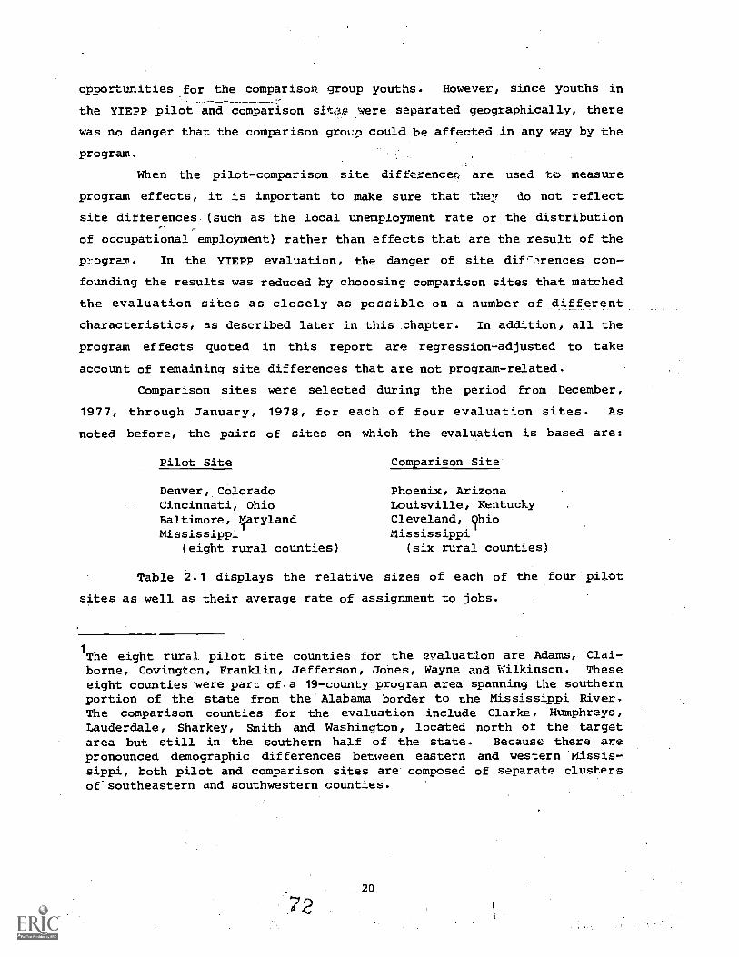
opportunities for the comparison group youths. However, since youths in

the YIEPP pilot and comparison sitew were separated geographically, there

was no danger that the comparison group could be affected in any way by the

program.

When the pilot-comparison site difft.rencen are used to measure

program effects, it is important to make sure that they do not reflect

site differences (such as the local unemployment rate or the distribution

of occupational employment) rather than effects that are the result of the

grogra:m. In the YIEPP evaluation, the danger of site diV,rences con-

founding the results was reduced by ch000sing comparison sites that matched

the evaluation sites as closely as possible on a number of different

characteristics, as described later in this chapter. In addition, all the

program effects quoted in this report are regression-adjusted to take

account of remaining site differences that are not program-related.

Comparison sites were selected during the period from December,

1977, through January, 1978, for each of four evaluation sites. As

noted before, the pairs of sites on which the evaluation is based are:

sites

Pilot Site

Denver, ColoradoCincinnati, OhioBaltimore, larylandMississippi

(eight rural counties)

Table 2.1 displays the relative

Comparison Site

Phoenix, ArizonaLouisville, KentuckyCleveland, 9hioMississippi

(six rural counties)

sizes of each of the four

as well as their average rate of assignment to jobs.

1

pilot

The eight rura1 pilot site counties for the evaluation are Adams, Clai-borne, Covington, Franklin, Jefferson, Jones, Wayne and Wilkinson. Theseeight counties were part of.a 19-county program area spanning the southernportion of the state from the Alabama border to the Mississippi River,The comparison counties for the evaluation include Clarke, Humphreys,Lauderdale, Sharkey, Smith and Washington, located north of the targetarea but still in the southern half of the state. Because there arepronounced demographic differences between eastern and western Missis-sippi, both pilot and comparison sites are composed of separate clustersof-southeastern and southwestern counties.

?,220

Table 2.1. Number of Youths Working in YIEPP Jobs

Pilot Sites

Number ofyouthsenrolled

Percentassignedto jobs

Baltimore 17,764 93.3

Cincinnati 5,632 90.3

Denver 4,301 84.0

Mississippi Pilot 13,291 95.2

'Total 404988 91.8

Source: Diaz et al. (1982: Table IV-1).

This ratio is the number of individuals who participated injobs divided by the number of individuals enrolled. These

data are derived from the Local Field Survey.

21

Cohort Effects. A principal goal of this analysis is to use data

from the YIEPP projects in the four pilot sites between 1978 and 1980 to

estimate the effects of, a potential national program. This national

program can be imagined in a steady state (having passed beyond start-up

difficulties), which youths below age 16 can count on as being available to

them as they pass through ages 16 to 19 until they graduate from high

school. Ideally, one would like to predict various outcome measures- -

program participation, school enrollment, high school graduation, employ-

ment and unemployment--on the age profiles for youths as they age into and

through program eligibility. This is a difficult undertaking, however.

The sample was constructed in the spring of 1978 and included youths aged

15 to 19 at that time. Since program operations were also beginning at

that point, much of the sample was beyond the age of initial eligibility

when the youths first heard of it. Thus, they may already have made

decisions and undertaken actions that would have been different if YIEPP

were available or if they had known it would at least be available to them

when they turned 16. For this reason, the cohorts aged 15 and 16 at

baseline provide the best indicators of the effects of a continuing na-

tional program. Particular attention is paid to these cohorts in the

chapters that follow.

The Longitudinal Survey

Samples of youths who were eligible for YIEPP, or would have been

eligible had a program been operating in their area, were selected at each

of the four pilot and comparison sites. The evaluation sample was drawn

during February and March, 1978, at which time a stratified random sample

of over 130,000 households was screened to identify eligible youths.

Subsequent baseline interviews were completed during the period from March

through August, 1978, with 7,510 eligible youths at the eight sites.

Interviews were also completed with the parents of these youths.

After the baseline wave of interviews had been completed, there was

further change in the composition of the longitudinal sample because

Congress extended the YIEPP demonstration beyond its original 18 months. A

fourth wave was added to the originally planned three-wave survey, allowing

22

7

the sample to be followed for a Longer period of time and permitting a

substantial postprogram period of observation. In order to add the

additional wave, however, without a corresponding increase in budget, the

original sample was reduced in size. Youths who had already become ineli-

gible for YIEPP by June, 1978--either by aging out,of eligibility or by

graduating from high school--were eliminated from the follow-up survey

wave. This brought the size of the baseline longitudinal sample-to-6,501,

which was not a serious curtailment from a design point of view. The

youths eliminated had had only three months to join YIEPP and, even if they

had joined, there is,00 brief a program experience for any effects to be

expected.

The first follow-up survey (Wave II) was conducted in the fall

of 1979, with the second follow-up wave of interviews (Wave III) taking

place in the fall of 1980. A final interview wave (Wave IV) was conducted

during the fall of 1981.

By the end of Wave III, the total completed- sample of youths was

4,749 (73.1 percent of the original baseline), with most of the attrition

occurring at the time of the Wave II survey. The completed Wave III sample

was, in fact, three subsets of the original longitudinal sample. By far

the largest group, numbering 4,033 youths, had remained in the target areas

either of the YIEPP pilot sites or comparison sites throughout the research

period. These youths maintained their program eligibility during the

entire_demonstration_period, at -least on the geographic criterion. In each

follow-up year, they completed an extensive local field survey instrument,

creating the continuous longitudinal history from January, 1977, to Septem-

ber, 1980, on which this report is based.

The second group consisted of 388 youths in the sample at baseline

who had moved out of one of the evaluation sites at sometime during the

aemonstration. These youths had completed the regular questionnaire as

long as they lived in the site. Although their move caused them to lose

their eligibility for YIEPP, these youths were administered a telephone

follow-up questionnaire (the Remote Movers Survey) which, though somewhat

briefer than the field instrument, also provided a continuous longitudinal

history of the critical dimensions of employment, schooling, and other

experiences.

23

The third group was a subsample of nonrespondents to Wave II, who

were reinterviewed in Wave III. A total of 1,674 youths failed to respond

to Wave II, but 378 of them completed the Wave III questionnaire focusing

upon the key dimensions of experience over the two-and-a-half-year period.

Thus, a continuous history has also been constructed of a nonrespondent

sample, which is particularly important 7 a consideration of nonresponse

bias issues. Since resource constraints made it impossible to reinterview

all the nonrespondents to the Wave II survey, the subsample chosen for

reinterview focused upon the principal sample target groups eligible for

YIEPP. It includes (a) black youths from Baltimore (the largest study site

with the largest number and concentration of-black youths) and its compari-

son site (Cleveland); and (b) Hispanic youths from Denver and its compari-

son site (Phoenix), that together were the sites where the overwhelming

majority of sample Hispanics resided at baseline.

In addition to the longitudinal survey data, school records were

collected on the analysis sample at two points during the demonstration:

summer through fall of 1979, and summer through fall of 1980. The informa-

tion was assembled for a four year period beginning with the 1976-1977

school year and ending with the 1979-1980 school year. These data included

attendance and tardiness information, courses pursued, grades and standard-

ized test score results.

Analysis Sample

The analysis sample for this report is the group of 4,033 youths

who completed the first three successive interview waves and remained in

the sites. The analysis is restricted to this group in order to provide a

study sample that has an invariant composition among the extensive inter-

related analyses presented below. Comparisons can thus be made with less

ambiguity. The effect of this strategy is to reduce the sample size on any

given subgroup or sample period as well as contribute to the possibility of

attrition bias. However, the reduction in sample size is generally too

small to affect statistical precision. Tests for attrition bias are also

performed throughout the study.

The basic demographic characteristics of this sample at baseline

are presented in Table 2.2. As shown in the table, minority representation

24

6

Table 2.2. Characteristics of the Analysis Sample at Baseline

Race: Highest grade attained:

White 13.7% ( 8th 24.3%

Black 76.2% 9th 22.1%

Hispanic 10.1% 10th 22.5%

11th 30.8%

Sex: 12th 0.3%

Male 46.3%

Female 53.7% Mean grade attained,

June 1978: 9.44

Age as of June 1978:

15 19.3% Worked at all, January

16 32.0% 1977 - March 1978:

17 24.8% Yes 49.2%

18 13.7% No 50.8%

19 10.2%

School status as of

Percent of time working,

January 1977 - March 1978: 14.4%

March 1978:

In-school 76.8% Marital status,

Out -ofschool 23.2% March 1978:

tr: Married 1.5%

Type of school: Separated or

Regular public 90.1% divorced 0.5%

Alternative public 4.0% Never married, 98.0%

Private or parochial 1.6%

Other 4.3% Number of children

March 1978:

Type of program: 0 85.9%

General 80.2% 1 11.8%

College preparatory 4.6% 2 2.0%

Vocational, commercial >2 0.3%

or business 11.4%

Other 3.9% Living with neither

natural parent,.

Degree sought: March 1978: 11.7%

High school degree 90.7%

GED 4.0% 1977 family income $5,305

None 5.3%

!=......y..1=11111Note: All statistics in this table are based on the 4,033 observations in the Analysis Sample.

lI

in the sample was very high--86.3 percent--a factor partly caused by the

inner city or southern rural location of sample sites, but also a function

of the greater representation of minority families among the low income

(and thus YIEPP-eligible) population. More than three out of four sample

members were black youths. Black youths far outnumbered other groups in

all the evaluation sites except Denver and Phoenix. Denver and Phoenix, by

contrast, jointly accounted for over 93 percent of the Hispanic youths in

the analysis sample.

More of the analysis sample were young women (53.7 percent) than

would be suggested by national population data. The reason for this, as

discussed later in this chapter, is that sample attrition was somewhat

higher among the young men than among the young women.

Over three-quarters of the sample was enrolled in school in March,

1978. The median age was just over 17. School attachment at baseline was

strongly and consistently related to age, with almost 92 percent of the 15-

and 16-year-olds, but only 46 percent of the 19-year-olds, attending

school. Consistent with national trends, school attachment was highest.

among black youths and lowest for white youths. Most youths who were

enrolled in school attended regular public schools in courses leading to a

high school diploma. About one in eight was taking a commercial, voca-

tional, or agricultural program. Only 4 percent of the school enrollment

periods reported during baseline interviews were leading to a GED degree,

and only 1.5 percent of the sample was in private or parochial schools.

Although school attachment in the spring of 1978 was reasonably

high, grade attainment was lesis impressive. Almost half of the analysis

sample had completed no more than the ninth grade, while only about three

in \ten had completed eleventh grade or better by June of 1978. Grade

attainment, as one would expect, also varied by age. Fifteen-year-olds,

who in the nation as a whole have typically attained at least the ninth

grade, had a mean attainment of 8.8 grades, with about one-quarter of

the group having less than a ninth grade education. As age increased,

relative grade attainment decreased. The mean grade attainment for 16-

through. 19-year-olds was 9.3,9.7, 9.8 and 10.1, respectively, with the

effects of reduced school attachment increasingly influencing grade

7926

achievement. There were some small differences in grade attainment at

baseline by race, with Hispanics (at 9.7 years of schooling) having ad-

vanced marginally farther than both blacks (with 9.4 years) and whites

(with 9.2 years). Moreover, females had a slightly higher baseline grade

attainment of 9.5 years compared to the male baseline grade of 9.2 years,

even though female sample members were slightly younger than their male

counterparts.

Overall, more than one-half the sample was below expected grade

level by June, 1978, including three-quarters of the 18- and 19-year-olds.

Over 24 percent of the sample were at least two full grades below normal

level, including over 40 percent of the 18- and 19-year-olds. Not sur-

prising, in-school youths had a higher grade attainment than those not in

school, with mean grade completed ranging from 1.4 to 1.6 grades higher,

depending upon the age cohort. Even among in-school youths, however, 34

percent had not completed the grade level usually expected for their

age.

About one-half of the sample had worked at some job during the

period prior to baseline (January, 1977 - March, 1978).1

Work experience

during this period was particularly likely for youths in Denver (68.6

percent), Phoenix (63.2 percent), and Cleveland (63.4 percent). It was

also unusually frequent among Hispanics (65.1 percent)--most of whom

resided in the strong labor markets of Denver and Phoenixand for males.

If a more comprehensive way of looking at labor force attachment is

used--the total number of days worked as a proportion of the total number

of days available for work--the picture of preprogram employment is not

greatly altered. Overall, the average sample member worked 14.4 percent of

the time in 1977, a bit more than one day per calendar week. Labor force

attachment was highest in Denver and Phoenix, but was also above average in

Cleveland and Cincinnati. Prior work experience during 1977 was a direct

function of age, with 15-year-olds working only occasionally (8.6 percent

of the time) and 19-year-olds working somewhat more (24.6 percent of the

time). Males worked almost twice as much as females.

1 A job was defined as working for pay for at least 10 hours per week forat least two consecutive weeks.

27

-Whites and Hispanics spent' substantially more of their, time working

than blacks--22.3 percent and 21.3 percent, respectively. The Hispanic

figure, however, is almost entirely a function of Hispanic concentration in

the two strongest labor markets, Denver and Phoenix. At the other sites,

Hispanics worked considerably less--only 8.3 percent of the time. Overall,

black youths worked only 12.1 percent of the time, a phenomenon that is

related in part to the higher degree of school attachment among black

youths.

Total family income for the sample was low, averaging $5,305 per

year in 1977. Mean annual family income was highest in Denver and lowest

in'rural Mississippi. It was also lower for black youths than for whites

or Hispanics.

Less than one in eight sample members was living with neither of

his or her natural parents. As would be expected, the frequency of this

family living condition was also directly related to age. Only 2 percent_

of the sample had ever been married at baseline, but .one-quarter of those'4.

who had been married were already separated or divoiCed. Marriage was

particularly rare among blacks. At baseline, only 0.4 percent of the black

sample members were married, compared to 3.9 percent of Hispanics. and 6

percent of whites. The infrequency of marriage, however, is not unusual in

a sample of youths whose median age was only just over 17, and in which

over three-quarters were 17 or less. More surprising is the number of

parents. Almost one out of seven already had children in the spring of

1978, and one in six of these teenage parents had more than one child. The

incidence of children was not strongly related to race, but was strongly

related to sex and age. Only 4.3 percent of youths aged 15 or 16 had

children, but over one-quarter of those aged 19 were parents. Likewise,

females were more than four times as likely to report having had children

as males. The rate of reported parenthood was highest among 19-year-old

females, at 45 percent.1

The high incidence of childbearing among female sample members should

.be kept in mind when considering the findings presented in later chapters.

Because of the pilot/comparison group design, the estimated effects of_

the program will not be affected. However, the high incidence of child-,

bearing may affect the absolute levels of such behavior as school and

labor force attachment.

28

8

For demographic variables that change over time, it is informative

to exa:slir,e changes over the three survey waves, as shown in Table 2.3. By

the fall *of 1980 (when the median age of t14 analysis sample was 19-1/2

years old) more than 90 percent had still never been married, but as the

sample aged, more had become married and/or divorced. The ratio 'of

marriage to divorce or separation was'about four to one. Childbearing

increased more dramatically with age. By Wave over one-third of the

sample had children. AlmOst 9 percent of the sample had two or. more

Children. Also, by the fall of 1980, more than one-quarter of the sample

was no longer living with either parent.

It is helpful to have a point of comparison inan interpretation of

the results of the YIEPP analysis sample in light of these sample charac-

teristics. Comparisons with the National Longitudinal Survey of Young

Americans (NLS) national probability sample--both for 15- to 19-year-old

poverty youths in their national probability sample and for all youths in

that age group--are presented in Table 2.4.1

As can be seen, the YIEPP eligibility criteria caused its sample

characteristics to be different from those of the general youth population.

Two factors stand out." First, the minority proportion of the YIEPP sample

was much :higher than for youth or poverty youth nationwide. The YIEPP

difference reflects the deliberate selection of YIEPP sites in areas with

concentrations of minorities, as well as residents below the OMB poverty

level. Second, the YIEPP sample was noticeably younger than either of its

NLS counterparts. Both this and the sharply different distribution by

grade attainment were a consequence of YIEPP sample truncation due to

ineligibility of high school graduates or possessors of GEDs.

The strong differences in acv, and race explain several of the other

patterns in Table 2.4. '..he younger and more heavily minority YIEPP sample

members were less likely to be married, less frequently living separately

from parents, and more likely to be in school. This is consistent with the

\relationships already observed in the sample between age and race, on

1 We are indebted to Dr. Michael Borus, Director of the Center for Human.Resourcejtesearch at Ohio State University, for providing these data andfor interpreting them to our research staff.

82

Table 2.30 Marital and Parental Status of the Anlysis Sample Oil6f Tire

Wave I

Spring 1978.Marital status:

,1=1.1.1,111y

Married 1.5%

Separat(24 or divorced 0.5%

Never married 98.0%

Parental status:

No children 85.9%

1 child 11.9%

2 children 2.0%

> 2 children 0.2%

Living with neither

natural parent 11.7%

Median age of sample

Wave II

Fall 1979

Wave III

Fall 1980

4.4' 7.7%

Cat 1.9%

99% 90.4%

.M.6% 66.3%

18.1% 24.9%

4.1% 6.8%

WA 2.0%

:19.441

17 yrs, 1 month 18 yes, 6 months

27.2%

19 yr$, 6 months

Table 2.4. The YIEPP Sample Compared with theNational Longitudinal Survey of Young American Samples

YIEPPanalysissample

1978 NLS Samplea

Poverty youths All youths

Race:

White 13.7% 48.2% 80.0%

Black 76.2% 38.3% 13.7%

Hispanic 111.14 13.5% 6.3%

Age:

15 19.3% . 20.2% 20.3%

16 32.0% 21.0% 20.7%

17 24.8% 21.0% 19.9%

18 13.7% 17.8% 19.5%

19 10.2% 20.0% 19.6%

Sex:

Male 46.3% 49.4% 51.3%

Female 53.7% 50.6% 48.7%

School statusMarch 1978:

In school 76.8% 71.3% 77.7%

Not in school 23.2% 28.7% 22.3%

Highest grade attained.June 1978:

< 8 24.3% 12.8% 4.7%

9 22.1% 16.0% 11.5%

10 22.5% 24.3% 23.7%

11 30.8% 15.8% 20.9%

>12 or GED 0.3% 31.1% 39.2%

Mean grade attained,June 1978 9.44 9.45 9.96

Marital status,Spring_1978:

Married 1.5% 5.2% 4.5%

Not married 98.5% 94.8% 95.5%

Children:

res 14.1% 12.6% 4.3%

No t5.9% 87.4% 95.7%

Living with neithernatural parent 11.7% 31.7%2 20.4%

b

Mean family incomec $5,305 $4,228 $20,975

aSpecial run of data from Wave I of the National Longitudinal Surveyof Young 4varicans by the Center for Human Resource Research at

Ohio Sta'-, .:iversity.bIncludes youths in college, which are 4.4 percent and 7.2 percent,respectively, P.!t the two NLS samples.cMean family inav figures are for calendar year 1977 for theYIEPP sample, caiurilar year 1978 for the NL8 sample.

The "poverty" sample of the NLS was derived by applying the 1978 OMBpoverty 'standard to the sample. This is also the standard used in the

YIEPP sample. However, it was only possible in this run to apply the

OMB standard for urban families. Thus, rural members of MS Youthsamples are somewhat overrepresented in the poverty sample, since OMBpoverty standards for rural areas are lower than for urban areas.

31 84

the one hand, and school attachment marriage on the other. Despite

their youth, YIEPP sample members were parents more frequVntly than either

of the NLS samples. The concentration of the YIEPP sample in poor inner

city areas may explain this difference, as well as the fact that the

incidence of childbirth increases rapidly over time.

Total family income for the YIEPP sample was 25 percent higher than

for the NLS poverty youth sample, although it was about four times lower

than the mean for youtl-s nationally. The difference is, in fact, greater

than that shown in Table 2.4, because the NLS data are for the calendar

year 1978, while YIEPP data are for the calendar year 1977, although

the overestimate is somewhat muted by the fact that the YIEPP estimate

included the value ct.,Food Stamps while the NLS figures do not. 1The

explanation of any remaining difference is not entirely obvious, but it

probably rests heavily on the fact that minorities were overrepresented in

the YIEPP analysis sample. It may also be, however, that YIEPP sites were

not representative of the national poverty population on total family

income.

Pilot and Comparison Sites

,MDRC and the Department of Labor chose the pilot sites for the

evaluation in December, 1977, based upon several general criteria. First,

since the research focus was upon broad-scale implementation to test an

entitlement model, the sites had to be chosen from the larger-sized Tier I

group. Second, at least one rural site was considered important,.a crite-

rion leading to the choice of the rural Mississippi program. Third,

geographic diversity was desired, increasing the likelihood thal. one east

coast site (Baltimore or Boston), one central site (Cincinnati or Detroit)

or one western site (Denver or King- Snohomish) would be included. Fourth,

the projected costs of data collection were important, playing a part in

screening out sites where family income made it likely that eligibility

rates would be relatively low, thus increasing the screening costs of

sample selection. Denver's strong labor market was therefore a negative

factor on that point, but the fact that Denver had the only Hispanic

population concentration among Tier I sites and was a site with a strong

1Food Stamps accounted for $784 of total annual family income of the YIEPPanalysis sample at baseline.

32

labor market made it desirable for purposes of representativeness and

brought Denver into.thesample. Boston was eventually excluded from final

consideration because, at the time sites were selected, there was still

major uncertainty on how long the Boston program could be funded. The

exclusion of Boston helped screen in Baltimore, which was also attractive

because it was a partial city site (it was desired that one study site be a

partial city) and was thought to have dynamic leadership. The choice of

Cincinnati aver Detroit as the geographically central site was influenced

by the fact that Detroit was a partial city site and the partial city site

of Baltimore had already been selected.

The four. YIEPP pilot sites chosen for the evaluation were not,

therefore, chosen to be closely representative, either of the YIEPP demon-

stration as a whole or of the nation. How they, in fact,'-compared on the

dimensions of unemployment rate and racial composition is shown in Table

2.5. The four-site average is similar in unemployment rate to the national

average in 1977. However, the racial vimposition of the sites varies to a

significant degree both within the four evaluation sites and in comparison

to the national average.

Generalizing from the results reported in subsequent chapters to

either the demonstration or the 'nation as a whole, therefore, should be

done cautiously, especially as tse results will be shown to vary both

with local labor market conditiov.s and for different racial groups. With

this in mind, the impact evaluation considers each pilot. site (or pilot/

comparison pair) on its own terms as revealing a great deal about what

happens when a program is introduced into a particular environment.

Three-site or four-site aggregations are used mainly as the most straight-

forward way of expressing the average program impacts at the designated

evaluation sites.

The selection of comparison sites was systematically aimed at

obtaining the closest possible match for each of the YIEPP sites chosen for

the evaluation. Pairs were matched on the, following dimensions:

Population

Size of labor market

Population growth, 1970-75

33

06

Table 2.5 Inv. Evaluation Sites Compared to YIMPF Total and the Nation

Site Unemployment rateRacial composition ofpopulation

Baltimore

Cincinnati

Denver

Mississippi

YIEPP evaluation sites( unweighted average)

11.39

7.0%

6.9%

4.2%

7.1%

(1976)a

(1977)b

(1976)b

(1977)c

15% white,

72% white,

91% white,

60% white,

859 nonwhite

28% nonwhite

91 nonwhite17% Hispanic

40% nonwhite

d

(1977)

(1970)

(1978)

(1975)

Boston

Detroit

Xing-Snohomish

Total non-study Tier I sites(unweighted average)

9.8%

13.1%

6.7%

8.8%

(1977)b

(1977)b

(1977)b

77% white,

30% white,

90% white,

22% nonwhite1% other (1970)

70% nonwhite (1977)

10% nonwhite (1979)

d

Tier II sites (unweighted average) 9.9% d

-program (unweighted average) 8.61 d

Nation 7.0% (1977) 89% white, 11% nonwhite5% Hispanic

(1910)

&-Jurces: manpower Demonstration Research Corporation (1977, Table 1); U.S.Department of Commerce (1978); and U.S. Depl3rtment of Labor (19H1).

aRates shown are for the city.bRates shown are for the prime sponsor area.

cRates shown are for the state.

dNot estimated.

8734

Unemployment rate

Labor market distribution of jobs

High school dropout rate

Ethnic distribution of population, particularly theyouth population

Characteristics of the poverty population

In Table 2.6, a number of these characteristics that are arrayed

for the pilot and comparison sites are relatively close. In Mississippi,

for example, the pilot and comparison sites hardly differed along any

measure except size,. The size difference should not to be surprising,

given that more weight was attached to the match on ethnic mix, percent of

families below poverty, and unemployment rate, than on'size of population

and labor force. Particular attention was paid to the institutional and

procedural similarities of the match, particularly as these applied to

school syEtems.

The Cincinnati-Louise i-lie ma oh was a good 0114-' on k%:pulation

change, percent of families in poverty, ethnic mix; p.ncent of -16- to

17-year-olds in school , unemployment rate, and labor riqt--tiloution--

although there were differences in the proportion of olet. 7.1t.hs in school

(in 1970) and in size. The Balleveland match was somewhat less

close, though still good. Both *..!c,ik 1:4:1ining industrial cities in the

eastern portion of the country lirktiti."4:titutial black populations and about

the same size labor forces, proport of families in poverty, and percent

of Wniths in school. Baltimore, however, had a larger central city, a

slower rate of population decline and a higher black population, especially

in the YIEPP target area. The only alternative as a comparison site,

however, was Washington, D.C., which was ruled ;:mt because the government

sector so heavily dominates the labor force. 'inere were also differences

between Washington D.C. and Baltimore in percent in poverty, school enroll-

ment, and the unemployment rate.

The Denver-Phoenix pair was an unsatisfactory-matchin--terms of

both size of population and rate of growth. However, they are both young

sunbelt areas with very similar proportions of Hispanics (at least in

1970). The match was also not entirely satisfactory on the unemployment

35

88

Population

July 11 1975

Population

change

1970.1975

Denver 484,500 - 5.91

Phoenix 664,700 12.91

Cincinnati 412,600 -9.01

losieville 336,000 - 7.11

Baltimore 851,700 - 6.01

Cleveland 638,800 -14.91

Kisolosippi Pilotb

167,200 2.31

Killioeippi Comparisone 195,900 2.01

United State' 213,030,000 4.81

Table 2.6. Selected Characterietice of the Pilot and Comparison Sites

Families with

money income

below poverty

level, 1969

9.4

8.8

12,8

13.0

14.0

13.5

38.5

37,3

10.7

Percent

black

1970

Percent

Spanish

surname

1970

Percent enrolled Unempllyment

in school, 1970 rate, 1977Wholesale

Total Manufacturing sl retail Government

16-17 18-19 SKS&

11.0 16.8 89.4 52.8 5.9 670,200 15.7% 25.21 18.21

7.0 14.0 86.0 52.3 7.4 490,300 17.1% 26.2% 18.31

27.6 0.6 83.6 60.0 5.6 562,100 28.71 23.11 14.11

23.8 0.4 83.3 46.2 5.2 172,400 28.71 22.31 14.2%

46.4 0.9 84.4 49.6 6.7 864,900 18.61 22.8% 22.3%

38.3 1.9 87.6 46.8 5.9 880,900 30.71 22.9% 1316

49.4 (0.1 na na 7.0

a

32,300 45.31 21.91 20.21

45.3 (0.1 na na 7.1

a

43,500 31.91 25.91 18.21

11.1 5.1d

90.0 47.7 8.2 90,546,000e 22,61 20.7% 11.21

.0.11.1.=11.M.011=1.1Note: Unless °therein noted, itatiatice in the above table are for the central city or for Mississippi, the cluster of

counties,

e1976 data.

bite Misoiseippi pilot counties are: Adams, Claiborne, Covington, Franklin, Jeffereon, Jones, Wayne and Wilkinpon. The Missiesippi controlcounties are: Clarke, Humphrey., Lauderdale, Sharkey, With and Washington.

c

For the six cities, repotted employment is for the SKSA for1977; for the Mississippi counties, employment is measured Et those workers

covered by Social Security, by induatry sector, as of March 12, 1976

d

Data are for calendar year 1976.

Oeta are for calendar year 1977.

Source: fill Department of Commerce (1978)1 U.S. Department of Labor (1961)1 .::ta U.S. Department of Libor (1981).

Ju,

rate. The school enrollment data were very similar. In any case, San

Jose, the closest alternative to Phoenix, was a much worse match. San Jose

was smaller, faster growing, located in a different, region, more heavily

Hispanic, and with a different school enrollment profile.

In addition to area matching, it is also important to match charac-

teristics of the sample members. Table 2.7 below shows basic demographic

information on the analysis sample.

The two rural Mississippi site samples matched extremely well,

particularly on ethnic mix,, age, school status in March, 1978, mean grade

attainment, marital status, and parenthood. Mean family income in 1977 was

higher in the comparison site, but both samples had lower incomes than

their urban counterparts (except for Louisville). Both Mississippi samples

were also slightly younger, more school attached, and had less recent work

experience than sample youths at other sites. The one difference between

the two sites in Mississippi was that the comparison sample was strongly

dominated by female eligibles.

The Denver and Phoenix samples were quite similar in sex composi-

tion, age, percent of time working, mean grade attainment and parenthood.

They were also reasonably similar in March, 1978 school status and income.

The racial compositions of the two were not very similar, but they both

had a majority of Hispanics and together accounted for almost 95 percent of

the Hispanic eligibles in the analysis sample. The two site samples were

also similar in having more work experience, a higher rate of marriage, and

higher income than the eligibles at the other study sites.

The samples in Baltimore and Cincinnati were both dominated by

black eligibles whose age, school status, marital status, and 1977 total

family income profiles willre very similar. Both sites had more school

attachment and a higher proportion of blacks than samples at the other

urban sites. The Baltimore sample, however, was heavily female, and, as a

consequence, had less preprogram work experience and was more likely

to have children than the Cleveland sample.

The analysis sample match was least close in Cincinnati and Louis-

ville. Family income was reasonably similar, but in comparison to Louis-

ville, the analysis sample in Cincinnati had a higher proportion of blacks,

Table 2.7. Analysis Sample Characteristics of Pilot and Comparison Sitesa

8-site 6-siteb

Mississippi Mississippi Total Total Total TotalDenver Phoenix Cincinnati Louisville Baltimore Cleveland Pilot Comparison Pilot JZomparison Pilot Comparison

Race:

White

Black

Hispanic

Sex:

Male

Female

Age, June 1978:

15

16

.17

18

19

School status,

'March 1978;

In school

Not in school

Worked at all,

January 1977 -

March 1978;

Worked

Not worked

Percent time

working,

January 1977 -

March 1978;

Mean grade

attained:

Marital statuai

March 1978;

Married

Separated or

divorced

Never married

Number of

children,

March 1978;

0,

1

2

>2

Mean family

income for

1977

N

14.2% 20.51 16.2% 31.41 4.7% 12.01 13.41 10.4% 11.0% 19.9% 10.2% 19.8%30.8% 18.4% 82.9% 68.2% 94.3% 86.11 86.61 89.21 78.8% 70.4% 89.01 79.3155.0% 61.1% 0.9% 0.4% 1.01 1.9% 0.0% 0.4% 10.2% 9.31 0.81 0.9%

48.3% 46.01 43.51 46.7% 44.81 49.2% 51.81 41.4% 46.41 4641 46.01 46.0151.7% 54.01 56.5% 53.3% 55.21 50.81 48.2% 58.6% 53.6% 54.0% 54.0% 54.01

17.0% 23.9% 20.9% 14:7% 20.3% 19.71 20.9% 16.31 20.0% 17.7% 20.61 16.6%32.91 28.81 31.31 33.7% 29.21 32.11 34.21 38.51 31.3% 33.7% 31.01 34.5125.11 26.11 24.61 21.3% 23.91 26.31 27.11 26.51 24.9% 24.5% 24.9% 24.3%14.21 10.31 13.11 15.8% 15.9% 11.1% 11.4% 11.9% 14.0% 12.9% 14.0% 13.3%10.8% 10.91 10.11 14.5% 10.7% 10.81 6.41 6.81 9.8% 11.2% 9.5% 11.31

71.3% 65.4% 76.9% ; 62.5% 80.7% 83.61 83.5% 81.8% 78.6% 72.8% 80.0% 74.1128.71 34.61 23.1% 37.5% 19.31 16.41 16.51 18.2% 21.4% .27'.21 20.01 25.91

68.6% 63.2% 51.9% 40.8% 47.5,4 63.4% 30.1% 41.41 48.9% 50.0% 44.7% 47.7431.41 36.8% 48.11'' 59.2% 52.5% 36.6% 69.51 58.6% 51.11 50.0% 55.3% 52.31

21.81 22.01 17.8% 13.0% 10.7% 17.91 9.0% 11.3% 14.11 15.2% 12.4% 14.01

9.8 9.7 9.2 10.2 9.3 9.7 9.9 9.8 9.5 9.5 9.4 9.A

2.31 5.41 0.91 3.5% 0.31 0.3% 1.7% 1.3% 1.0% 2.5% 13.8% 2.0%

1.0% 0.01 0.91 0.9% 0.11 0.01 1.11 0.0% 0.6% 0.3% 0.6% 0.4196.71 94.61 98.21 95.6% 99.6% 99.71 97.2% 98.7% 98.4% 97.2% 98.6% 97.61

88.7% 89.7% 85.61 79.4% 83.5% 90.2% 89.2% 86.5% 86.1% 85.4% 85.5% 84.7%10.11 9.2% 11.4% 16.01 14,3% 7.91 8.21 10.11 11.6% 12.31 12.0% 12.8%1.2% 1.1% 2.5% 2.41 1.81 1.6% 2.61 2.7% 2.0% 2.1% 2.2% 2.2%0.0% 0.0% 0.54 0.2% 0.4% 0.31 0.01 0.7% 0.3% 0.21 0.31 0.31

55,796 55,365 55,319 35,173 $5,402 $5,349 $4,696 $5,212 $5,318 $5,274 $5,159 $5,244

487 185 692 456 1060 317 539 297 2,778 1,255 2,291 1,070

a1110 111 fal,o kwAiho vhararrerlstics 4 the analysis sample.

52

was slightly younger and more attached to school in March, 1978. These

youths also had more prior work experience, the lowest mean grade attain-

ment of the sites (Louisville had the highest), and were less likely

to be married.

The four-site pairs were, thus, reasonably similar along seven;

though not always the same, dimensions. They were not, however, identical,

and the inevitable differences that remain have t.0 be adjusted for in the

analysis so that the results do, in fact, reflect differences attributable

to the YIEPP treatment. The results reported in the rest of this report

are thus regression-adjusted estimates.

In Chapters 4 and 5, for example, all the results labeled "program

effects" were obtained in the following manner: A regression model was

estimated using the sample of youths from both pilot and comparison sites

who were eligible for participation in YIEPP (or, in the case of comparison

sites, would have been eligible if a program had been operating there).

The outcome measure--for example, the employment/population ratio--was

specified as a-function of three sets of variables. The first set included

such demographic variables as age, race, and sex. The second set contained

person-specific variables related to the outcome measure. For example, in

the case of the employment/population ratio, a person's preprogram employ-

ment/population ratio would be used. The third set included a constant and

a site variable that equalled one if the youth lived in a pilot site and

zero otherwise. Program effects were estimated by the coe on the

0-1 pilot site variable. This method controls for differences in the other

variables (e.g. age, race, sex, preprogram employment/population ratio

etc.). Results of such analyses are presented in this report as "regres-

sion adjusted" findings.1

1In the example of the employment/population ratio in the fall of 1979,the estimated program effect is adjusted for differences between the sitesin 1977 in the demographic variables and employment/population ratios.The coefficient on the pilot site variable measures the average differ-ence in the outcolae measure between youths in the pilot and comparisonsites, controlling for differences in the other variables in the regres-sion equation. Using lagged values of the outcome variable is:particu-larly important to the goal of reducing site effects that can be eon-

----2

39'

Attrition from the Baseline Longitudinal Sample

The analysis sample of 4,033 youths, on which this report is based,

is 38 percent smaller than the baseline longitudinal sample of 6,501. As

noted above, this attrition is principally-due to nonresponse in the

Wave II and Wave III surveys (32.8 percent), some of which was caused by

the elimination of some interviewed sample members fror, the analysis frame

because they had moved out of the evaluation areas (5.2 percent). Wht

this attrition caused some changes in the composition of the sample; tests

for attrition bias generally indicated that 't.heee either was no bias

or that the bias may have resulted in some (small) understatement of,

program effect.

As illustrated in Table 2.8, the sample became somewhat younger,

blacker, and more female over time. This is a consequence of the fact that

the longitudinal response was poorest in Denver and Phoenix (heavily

Hispanic, with more than an average proportion of white youths). Longi-

tudinal response has been best in Mississippi and Baltimore (where blacks

were most heavily represented and where samples were slightly younger and

more female than the average). The different longitudinal response rates

by site also caused the distribution of the sample to alter across sites.

Baltimore, Louisville, and the two Mississippi sites gained, while Denver,

Phoenix, Cincinnati, and Cleveland lost. The pilot-comparison ratio of the

sample, however, did not change noticeably. In the longitudinal baseline

sample, 68.4 percent of the youths were at pilot sites; the comparable

percentage of the analysis sample was 68.9 percent.1

The analysis sample was somewhat more attached to school in March,

1978, than the baseline longitudinal sample and had slightly less prior

work experience. The difference in each case, however, was modest. Grade

attainment (both its mean and distribution) and childbearing behavior were

virtually identical for the two samples.

founded with program effects. 'To--the wctent, for example, that unem-ployment rates are consistently diffat:ent between pilot and comparisonsites, these differences in aggregate demand would be reflected in pre-program employment/population ratios and, therefore, adjusted for in the

estimates. of program effects.

1See Barclay et al, (1979: Chapter 3).

40

Table 2.8. Characteristics of Baseline Longitudinal

Characteristic

and Analysis Samples

Analysissample

Baselinelongitudinal

.sample

Race:White 17.2% 13.7%

Black 69.9% 76.2%

Hispanic 12.8% 10.1%

Sex:

Male 49.2% 46.3%

Female 50.8% 53.7%

Age as ofJune 1978:

15 14.7% 19.3%

16 30.6% 33.0%

17 26.9% 24.8%18 15.7% 13.7%

19 12.1% 10.2%

Site:Denver 16.0% 12.1%

9hoenix 6.8% 4.6%

Cincinnati 18.8% 17.2%

Louisville 9.9% 11.3%

Baltimore 22.9% 26.3%

Cleveland 8.3% 7.9%

Mississippi Pilot 10.9% 13.3%

MississippiComparison 6.4% 7.3%

School statusas of March1978:

In school 72.6% 76.8%

Out of school 27.4% 23.2%

Highest gradeattained, June1978:

< 8 24.0% 24.3%

9 23.0% 22.1%

10 22.5% 22.5%

11 30.2% 30.8%

>12 or GED 0.3% 0.3%

Percent timeworking, January1977-March, 1978: 15.8% 14.4%

Mean gradeattained, June1978: 9.49 9.44

Children:Yes 14.4% 14.1%

No 85.6% 85.9%

N 6,501 4,033

aFor more detailed statistics on this original sample, seeBarclay, et al. (1979: Chapter 3).

Whether changes in the sample composition may have affected impact

estimates is a testable hypothesis. Attrition bias may be estimated, as

mentioned, by using data from the sample of Wave II nonrespondents who were

interviewed in Wave III. The effects of this attrition have been noted

above. The specific analysis of attrition bias as it affects estimates of

participation, school enrollment, employment and labor force participation

is presented in Appendix C to this volume.

Program Eligibles

The dynamics of eligibility, and how this report deals with them

are complex and worthy of attention. Indeed, fundamental to an understand-

ing of this evaluation is a clear comprehension of what is meant by the

term "eligible" youth and an awareness of the difference between eligibles

and longitudinal sample members.

A stratified random sample of eligibles was selected early in 1978.

This encompassed youths from low income or welfare families, 15- to 19-

years old, residing in a program target area or defined comparison area,

who had not yet graduated from high school. Sample members were followed

over time with successive survey waves, even though their eligibility

status may have changed. For example, sample members who were less than 16

years old at baseline were not yet eligible for YIEPP, but aged into

eligibility. As they did so, the size of the program eligible population

in the sample increased. Also, some youths, over time, moved out of

program sites or designated comparison areas, becoming ineligible for that

reason, althOugh the Remote Movers Survey continued to collect data on

them. This kind of geographic movement, however, reduced the size of the

sample eligible population. Finally, since high school graduation or

becoming 20 years old made a youth ineligible for YIEPP, both graduation

and aging further reduced the size of the eligible population in the

sample.1 The number of eligibles in the sample, thus, changed constantly

over time.

1 There are three limitations to a literal application of the programdefinition of eligibility to the evaluation. First, one of the studysites--Baltimore--hada target area that did not encompass the entirecity. Movement of residency of sample members between the target areaand the nontarget area in Baltimore is not detected in the survey. It

42

The data base used In this report encompasses all sample members

who completed local field interviews in each of the first three survey

waves1 Different proportions of these youths were eligible for YIEPP at

different points in time, depending upon age and high school graduation. :-

For example, Table 2.9 shows the size and basic characteristics of the

eligible sample members at several points since the spring of 1978. The

numbers presented in this table adjust for aging in, aging out, graduating,

and moving out of YIEPP program eligibility.

The first observation of interest in Table 2.9 is the fluctuation

in the number of eligibles in the sample. Eligibles increased in number

through the fall of 1978, with very little drop-off in the spring of 1979.

During this period, sample members who were less than 16 at baseline aged

into the sample. There was little aging or graduating out, since youths

who had graduated or turned 20 by June, 1978, had already been eliminated

from the sample after baseline. At the peak, in the fall of 1978, over 95

percent of the Wave III analysis sample was eligible. After the spring of

1979, however, the number of eligibles declined regularly, as a function

1

is, therefore, possible that some youths in the Baltimore sample became

ineligible by dint of residence, but are not considered such in the

evaluation. Available evidence suggests that movement of this sort was

trivial. Second, since the sample was selected at one point in time, it

missed youths who may have become eligible later. This could happen in

two ways. First youths who were 14 and under in the spring of 1978 were

not sampled. Some became eligible for YIEPP late during the period of

program operations. Second, youths who may have moved into a designatedsample area after the sample was drawn are not included. Finally, family

income was only gathered during the baseline. Thus, it is possible that

youths who were eligible at baseline became ineligible because of family

income changed sometime after the spring of 1978. To the degree that this

occurred, it is not detected in the evaluation. Equally undetected is

income movement in the opposite direction. Youths who were ineligible on

income grounds at baseline, but may have later become eligible because of

income, were not sampled. While the magnitude of these movements cannotbe quantified, we believe that none of them could substantially affect the

results contained herein.

The analysis sample thus encompasses 85 percent of the sample of 4,749

who completed Wave III. It does not include 338 remote movers, who will

be examined as part of post-program impact analysis. It also does not

include 378 Wave II nonrespondents with whom interviews were completed in

Wave III. These two groups, are, however, included in the analysis of

attrition bias presented in this volume.

430-i

Table 2.9. Program Eligibles, Spring 1978 - Summer 1980

SummerSpring Summer Fall Spring Summer Fall Spring1978 1978 1978 1979 1979 1979 1980 1980

Number ofeligibles 3,118 3,428 3,840 3,759 3,377 3,037 2,890 2,403

Percent of Wave IIIanalysis sample (4033) 77.3% 85.0% 95.2% 93.2% 83.7% 75.3% 71.7% 59.6%

Pilot sites 68.4% 68.6% 69.1% 69.3% 69.9% 69.4% 69.2% 70.1%

Comparison sites 31.6% 31.4% 30.9% 30.7% 30.1% 30.6% 30.8% 29.9%

Sex:

Male 45.9% 46.6% 46.3% 46.4% 47.3% 48.2% 48.1% 48.8%

Female 54.1% 53.4% 53.7% 53.6% 52.7% 51.8% 51.9% 51.2%

Race:White 14.3% 14.0% 13.7% 13.5% 13.0% 13.4% 13.1% 12.9%

Black 75.7% 76.0% 76.0% 76.4% 76.6% 76.2% 76.4% 76.1%

Hispanic 10.0% 10.0% 10.3% 10.1% 10.4% 10.4% 10.5% 11.0%

Age at the time:16 43.6% 37.9% 38.4% 26.5% 16.2% 6.8% 1.1% 0.7%

17 29.6% 31.0% 30.5% 33.1% 36.9% 42.7% 33.7% 20.0%

18 16.2% 17.7% 18.3% 24.2% 27.0% 28.9% 36.0% 43.1%

19 10.6% 13.4% 12.8% 16.2% 19.9% 21.6% 29.2% 36.2%

SS

of aging, graduating, or moving out of eligibiiityv and the fact that the

sample no longer contained many youths who were aging into eligibility.

Thus, by the summer of 1980, less than 60 percent of the anslysifi sample

was still eligible, and by the summer of 1981, it is unlikely that much

more than 20 to 25 percent of the analysis sample 'was still eligible.

Since the final analysis Of YIEPP focuses on postprogram impacts, however,

most of the sample can b0 included in that analysis.

The eligible sample size pattern is mirrored by the changing age

profile of eligibles. Through the fall of 1978, a majority of the eligi-

bles (between 68.9 and 73.2 percent, depending on the time) were 16 or 17.

As time passed, the age of the eligible sample population.increased such

that, by the summer of 1980, almost 80 percent of the remaining eligibles

were at least 18.

In other key respects, the composition of the eligibles has changed

only slightly. In the spring of 1978, 68.4 percent of the eligibles were

at pilot sites. Two and one-third years later, pilot sites contained

70.1 percent of the remaining eligibles, a negligible change. The eligible

sample became slightly more male over time, but again the change is margi-

nal. The racial composition of the eligible sample was very stable over

time, though the white proportion dropped a bit. Overall, the eligible--

population remained remarkably stable since the spring of 1978 on the basic

demographic characteristics of sex, race, and site.

Summary

The design for this evaluation is based upon a comparison of

eligibles at the four YIEPP pilot sites and four comparison sites, relying

on longitudinal data from those sample members (4,033) who completed local

field questionnaires (LFS) in three successive waves of interviews: the

spring of 1978 (Baseline), the fall of 1979 (Wave 1I) and the fall of 1980

(Wave III). The pilot and comparison sites aftA samples match, on the

whole, relatively well, increasing confidence that estimates based upon....

pilot-comparison differences are not confounded by other effects. The

models that produce these estimates further control for, and thus net out,

differences in demographic and key site variables. While there has been

attrition in the sample since baseline, bias due to attrition does not

45

99

alter significantly the estimates presented in this report. Characteris-

tics of the sample of youths for this evaluation show that YIEPP was well

targeted on those likely to experience the problems it was desigaed to

address. Almost seven-eighths of the sample was composed of minority

youths, a much higher proportion than the national probability sample of

youths and of low income youths reflected in the NLS. As such, the YIEPP

target group is extremely vulnerable to the complex problems of high

unemployment rates, smaller earnings, and underachievement in education

discussed in Chapter 1.

While school attachment (as of March, 1978) was not below national

norms, this is probably a result of the fact that the YIEPP sample was

younger than average, due to the YIEPP eligibility criteria. Grade attain-

ment, however, was behind national norms, falling further behind as age of

the youths increased. Last, there was an unusually high incidence of

childbearing among sample members, a phenomenon which undoubtedly exacer-

bates the difficulty of educational progress and employment for this

group.

46

1 00

CHAPTER 3

PROGRAM PARTICIPATION

Introduction

In programs where sufficient funds are available to serve all

eligibles, as was in principle true for YIEPP, the extent and composition

of program participation takes on more than usual importance. Which youths

are employed in YIEPP jobs and the pattern of their subsequent program

experiences are key determinants of program impacts. Participation pat

terns also determine program costs. In our previous analysis (Farkas et

al. (1980: Chapter 2)) we found that YIEPP participation varied across

sites, over time, and by individual characteristics. In particular,

in-school youths were more likely than school dropouts, and not employed

youths were more likely than employed. youths, to participate in YIEPP.

These and related findings are an important aid in comprehending the

mechanisms underlying the program impacts on school and work reported in

Chapters 4 through 6 below. In this chapter we extend the analysis of

participation to the two and one-half year of full-scale YIEPP operations.

The discussion here complements the discussion in the MDRC Implementation

Reports (Diaz et al. (1982)), and definitively summarizes our participation

results for the period of YIEPP operations from the spring of 1978 to the

summer of 1980.

In this evaluation we are studying data from four of the seven Tier

I YIEPP sites. Of course, both local conditions and program implementation

success varied across these sites. As summarized in Chapter 1, the MDRC

implementation studies suggest that Denver an a relatively poor YIEPP

program, Baltimore ran an effective program, and Cincinnati and Mississippi

fell between these extremes. As we shall see, participation and other

site-specific findings strongly support this ranking.

Measuring Program Participation

YIEPP had four eligibility rules--the participating youth must

reside in a program area, must be between 16 and 19 years of age, and must

not have graduated from high school or completed the GED, and family income

47

must be below the poverty level. (See Chapters 1 and 2 above.) In this

report we restrict attention to youths who completed all three waves of the

local field survey in order to maintain a complete and consistent longitud-

inal data set for the analysis sample. While this results in differential

attrition for each time period analyzed and somewhat smaller sample sizes,

we conducted tests for attrition bias1

, which indicated that sample size

reduction was too small to affect the statistical precision of our esti-

mates. We then further restricted attention to program-eligible youths on

a period-by-period basis, separately for each season, from the spring of

1978 through the summer of 1980. Only youths who were income- and loca-

tion-eligible at the time of the screening interview in the spring of 1978

and who had not graduated from high school by the summer of 1978 were

included in the survey sample. In the analyses for this report we also

eliminated youths who subsequently moved out of the program (or comparison

site) area,2 plus those who were ineligible due to age or high school

graduation on a period-by-period basis: That is, we "aged" youths into and

out of eligibility separately by period,3 and youths "graduated" out cf

eligibility in the period following the one in which they received a high

school diploma or its equivalent. This restriction of the study sample to

program eligibles is more elaborate than the effort undertaken in our

previous report, so that the results reported here supercede previous

findings.

Program participants are defined as youths holding a YIEPP job for

at least two weeks.4

We do not count as participants youths who enrolled

1In order toanalyze datato Wave II ofWaves II andpriate in the

2That is, youths who moved sufficiently far from their city or town of

residence to receive a "remote movers" questionnaire.

test for potential bias due to sample attrition, we alsofrom an "attrition sample" of youths who failed to respond

the local field survey, and were then found and administered

III at a later date. These results are discussed as appro-

text; the underlying calculations are reported in Appendix C.

3Youths aged 15 or less in the spring of 1978 became eligible in theperiod during which they reached age 16; older youths became ineligible

in the period following the one in which they turned 20.

4For a description of the survey methodology used to identify YIEPPjobs,

see Farkas et al. (1980: p. 12 and Appendix A2).

48

1o2

but for some reason never worked at a program job for the minimum period.

These individuals never received the basic YIEPP treatment, a program job.

Therefore, the program is unlikely to have had any impact on their behav-

ior.

Program Participation Rates

This sdction reports program participation rates, defined as the

percent of program eligibles ever holding a program job for at least two

weeks during a particular analysis period. This measure is identical to

that employed in our previous report (Parkas et al. 1980: Chapter 2),

and where time periods overlap, our results are generally close to the

findings reported there. 1

In addition, these methods yield program

participation levels which are consistent with data from the YIEPP manage-

ment information system (EIS).2

Program Participation, Separately by Period. Table 3.1 displays

estimates of program participation rates for youths in the study sample

during each of the periods of full-scale program operations. Of course,

the age distribution and other characteristics of these youths change over

time, but the sample was fully representative of the eligible population at

the time it was selected in the spring of 1978, as well as during the

remainder of 1978 and the beginning of 1979, when 15-year-old sample

members were aging into eligibility. Further, by restricting attention to

youths aged 15 to 16 in the spring of 1978, and following their behavior.... ,

for the two and one half year period, subsequent analysis (Table 3.2) will

permit examination of the participation pattern exhibited by a cohort of

youths as it aged through the program. This, then, will yield estimates of

participation that-most closely represent what one would observe in an

ongoing national program.

1Small remaining differences are due to data cleaning and changes in thestudy Sample. In this report we restrict attention to youths who com-pleted three waves of the local field survey, and focus more elaboratelythan in previous work on those youths who were eligible for YIEPP duringeach analysis period.

2See Appendix A, Table A3.1 and Farkas et al. (1980: Appendix A2, pp.131-132). Note that the EIS comparison is a test of the reliability oflocal field survey self-reports, rather than a methodology for deter-mining participation,

49

103

Table 3.1. Program Participation Rates by Site and Period

Cumulative:Spring 1978through Spring Summer Fall Spring Summer - Fall Spring Summer

Summer..1980 1978 1978 1978 1979 1979 1979 1980 1980

All sites 56.2 24.8 33.4 34.4 37.8 38.8 30.0 32.1 28.4

(2,778)a (2,132) (2,353) (2,652) .(2,605) (2,362) (2,107) (2,000) (1,685)

Denver 38.8 16.9 24.7 23.2 25.0 25.2 15.1 14.1 12.5

(487) (384) (433) (475) (452) (425) (372) (357) (319)

Cincinnati 49.3 ' 14.0 22.4 28.1 3U.4 31.7 23.1 26.1 26.3

(692) (521) (577) (658) (649) (600) (541) (509) (461)

Baltimore 68.8 41.8 45.3 45.5 50.1 50.0 42.1 43.2 39.0

(1,060) (815) (894) (1,002) (988) (926) (794) (759) (664)

Mississippi 56.2 12.1 32.3 31.1 34.7 38.2 29.0 34.7 24.5

(539) (412) (449) (517) (516) (411) (400) (375) (241)

Note: Throughout this chapter, the sample includes youths who have completed all three waves of the Local Field Survey

in all four pilot sites. See Chapter 2 for further details. The participation rate is the number of youths

ever holding a program job for at least two weeks divided by the number ever eligible in each period. Youths

are defined as being program-eligible in a particular period if (1) they are age 16 through 19 and (2) they

have not graduated from high school or received the GED. All youths in the sample met the family income and

residential eligibility requirements as of the spring of 1978.

aNumber of eligible youths.

10.1

First, however, we focus on Table 3.1, which indicates participa-

tion levels at different points in time, as well as intersite differences

in these levels. The first column of the table shows cumulative partici-

pation rates--the percent ,of. (ever eligible) sample members who held a

YIEPP job for at least two, weeks. Among 2,778 sample members responding to

three waves of the local field survey, 56.2 percent participated in YIEPP

at some time. This is a weighted (by site sample size) average of 68.8

percent in Baltimore, 56.2 percent in Mississippi, 49.3 percent in Cincin-

nati, and 38.8 percent in Denver. These are high participation rates, and

suggest that the program achieved significant visibility and some impor-

tance for a large percent :'.ge of target population youths. They also lend

support to a key premise of the program, that many target population youths

wish to work but in the absence of YIEPP are unable to find jobs at the

minimum wage.

Also important in this table is the_low participation in Denver.

This is at least partly due to poor program implementation in this site

and the fact that intake ceased June, 1979 (see Chapter 1). These factors

are important determinants of the low or nonexistent program effects on

schooling and employment reported for this site in Chapters 4 and 5 below.

Thus, discussion of the special circumstances surrounding Denver will recur

throughout the analysis.

Reading across the first row of Table 3.1, we find period-specific

rates rising from 24.8 percent in the spring of 1978 to a high of 38.8

percent in the summer of 1979, and falling thereafter to 28.4 percent in

the summer of 1980. This pattern is largely due to the aging of the

sample, although variations in program administration over time also play

some role. The pattern over time is similar across sites, with period-

specific rates rising to a peak in the summer of 1979, and declining

thereafter in each site. Relative site participation rates are generally

stable over time, with Baltimore showing the highest rates, usually fol-.

lowed in order by Mississippi, Cincinnati, and Denver.

The Effect of Sample Attrition. It is useful to assess the effect

of sample attrition on these results. This can be done through study of

the attrition sample data. As described in Chapter 2, these data were

collected by restricting attention to Hispanics in Denver/Phoenix and

blacks

youths

sample

in Baltimore/Cleveland, and undertaking special efforts to locate

who dropped from Wave II of the survey. The resulting, attrition

was administered both Wave II and Wave III interviews at a later

date. Program participation rates for these and matching youths who

completed all three survey waves are reported in Appendix C, Table C2.1.

In all cases, program participation rates are estimated to be lower

for the attrition sample than for youths who completed all three waves of

the local field survey. Z,Imong Hispanic youths in Denver, 36.9 percent of

local field survey sample members participated in YIEPP at some time,

whereas for the matched attrition sample, the rate was 18.7 percent. Since

sample attrition was high in Denver, the estimated participation rate in

the absence of attrition (a weighted average of these two rates) is 27.8

percent-for Denver Hispanics, a significant decline from the local field

.survey rate. However, the participation pattern over time is the same for

the two samples.

Black youths from the Baltimore attrition sample also.show lower

rates than those for the comparable analysis sample, but here

crepancy is smaller. Cumulative program participation' rates

percent for the local field survey, and 61.7 percent for the

sample. When these are combined with the lower Baltimore sample

the dis-

are 70.5

attrition

attrition

rate, the estimated participation rate in the absence of attrition is 68.4

percent, a decline of only 2.1 percentage points from the local field

survey rate. Again, the time pattern,is similar in the two samples. Since

it is the Baltimore rather than the Denver experience which was typical of

data collection as a whole (see Jerrett et al. 1982), we are confident that

although correction for attrition somewhat lowers estimated participation,

it does not disturb the overall finding of high YIEPP participation.

Program Participation by Cohort. Table 3.2 displays participation

rates separately for sample members aged 15 to 16 and those aged 17 to 20

on June 1, 1978. This is useful because the behavior of the 15- to 16-

year -old cohort suggests the pattern that would be observed as successive

52

110

Table 3.2. Program Participation Rates by Cohort and Period

Fall1979

Spring1980

Summer1980

Cumulative:Spring 1978throughSummer 1980

Spring1978

Summer1978

Fall1978

Spring1979

Summer1979

Age in June 1978:

15-16 65.8 28.4 36.0 35.6 41.0 44.1 36.5 38.8 33.0

(1,435)a (789) (1,032) (1,377) (1,413) (1,368) (1,322) (1,318) (1,191)

17-20 46.0 22.7 31.4 33.1 34.0 31.6 18.9 19.1 17.4

(1,343) (1,343) (1,321) (1,275) (1,192) (994) .(785) (682) (494)

See note to Table 3.1.


10

cohorts aged through an ongoing national program. 1

For this group, the

cumulative participation rate is 65.8 percent, 9.6 percentage points higher

than the cumulative rate for the total analysis sample shown in Table 3.1.

This higher value is a better estimate of the true "longitudinal" rate

experienced by target population youths in an on-going national program.

Each period-specific rate for this group also reflects these elevated

participation levels, but the time pattern is as before, rising to a peak

during Summer, 1979, and declining thereafter. The peak occurs when these

youths are 16 to 17 years of age, supporting previous findings and program

MIS results suggesting that YIEPP is most attractive to younger indi-

viduals.

Not surprisingly, participation is lower for the 17- to 20-year-old

cohort, a significant percentage of whom have dropped out of school and/or

found non-YIEPP employment. The much higher rates for the 15- to 16-year-

old cohort are most appropriate for generalizing to a potential national

program. These rates leave the qualitative impressions of Table 3.1

unchanged--demand for and participation in YIEPP was very high among target

population youths.

Program Participation by Sex, Race, and Cohort. The first column

of Table 3.3 shows cumulative participation rates for sex and race groups.2

Females were slightly more likely than males to participate in the program.....

(57.1 percent versus 55.3 Percent), and blacks (63.4 percent)_were much

more likely to participate than Hispanics (38.3 percent) or whites (21.5

percent). However, since almost all Hispanics were in Denver, participa-

tion rates for this group are confounded with the Denver site effect.

In the full race/sex breakout, black females show the highest

participation rate (64.8 percent) followed by black males (61.7 percent),

Hispanic females (39.3 percent), Hispanic males (37.0 percent), white males

(24.1 percent) and white females (19.4 percent). These results are consis-

tent with the observation that in the absence of federal assistance,

minority and female youths experience the greatest difficulty finding

employment.

1In Appendix A, Table A3.3 these data are used to estimate annual programparticipation in an ongoing program, thereby providing results which canbe used to estimate the costs of a potential national steady state pro-gram.

2For period-specific rates for these groups, see Appendix A, Table A3.2.

54

Table 3.3. Program Participation Rates(Spring 1978 - Summer 1980) by Cohort.

Race and Sex

Allyouths

Youths age 15 to16 in June 1978

Youths age 17 to20 in June 1978

Male

Female

55.3(1,290)a

57.1

(1,488)

65.9(656)

65.7(779)

44.3(634)

47.5(709)

White .21.5 31.8 11.2

(303) (151) (152)

Black 63.4 72.5 53.4

(2,190) (1,147) (1,043)

Hispanic 38.3 47.5 29.7

(285) (137) (148)

White male 24.1 37.7 9.4

(133) (69) (64)

White female 19.4 26.8 12.5

(170) (82) (88)

Black male 61.7 71.3 51.4

(1,022) (530) (492)

Black female 64.8 73.4 55.2

(1,168) (617) (551)

Hispanic male 37.0 49.1 28.2

(135) (57) (78)

Hispanic female 39.3 46.3 31.4

(150) (80) (70)



55

The second column of this table shows similar participation pat-

terns across sex/race groups for the 15- to 16-year-old cohort. The

principal difference is that rates for the younger cohort are shifted

upward by 9 to 10 percentage points. Rates for the older cohort are

shifted downward, typically by a like amount.

Table 3.4 presents regression-adjusted estimates of the net effects

of site, cohort, sex, and race; for each of these variables the effects of

the others are (statistically) removed, and fitted participation rates are

shown as the variable in question changes value and the remaining variables

are held constant at their sample means. The key point here is that the

15- to 16-year-old cohort shows almost no change in its participation rate

after statistical adjustment, which gives further emphasis to the represen-

tativeness of its behavior in an ongoing national program.

The remaining results of Table 3.4 simply reinforce findings from

the unadjusted rates of Table Females are more likely to participate

than males (56.7 percent versus 55.5 percent), blacks are more likely than

Hispanics, Hispanics are more likely than whites (61.5 percent versus 48.5

percent versus 24.4 percent), and the sex/race categories show rates

similar to their unadjusted values.

Program Participation by Sex and Family Status. Table 3.5 shows

the effect of family status on YIEPRparticipatin. This table is con-

structed as follows. First, for the period of the spring of 1978 to the

summer of 1979, we identify those females who were (a) living with neither

natural parent, (b) married, or (c) had their own children at the beginning

of the period. (These categories are not mutually exclusive.) Then,

restricting attention to program eligible youths, we calculate program

participation rates for all females, and for females in each of these

categories. These calculations are repeated for males. Finally, the

entire set of calculations (including recalculation of family status at the

beginning of the period) is repeated for the period of the fall of 1979 to

the summer of 1980.

We find that each of thestatuses--living with neither natural

parent, married, or having children--depresses YIEPP participation. The

strongest depressive effect is associated with marriage, which reduces

YIEPP participation rates from the 35 to 50 percentage point range down to

56

Li 0

Table 3.4. Adjusted Program Participation Rates

Cumulative:Spring 1978throughSummer 1930

Denver

Cincinnati

Baltimore (reference group)

Mississippi

46.3**

49.6**

65.5

55.1**

Age in June 1978:

15-16 65.6**

17-20 (reference group) 46.1

Male (reference group) 55.5

Female 56.7

White 24.4**

Black (reference group) 61.5

Hispanic 48.5**

White male 26.9**

White female 22.5**

Black male (reference group) 60.2

Black female 62.8

Hispanic male 48.3**

Hispanic female 48.7**

Note: The probability of ever participating from Spring 1978 through Summer1980 was estimated as a function of site, cohort, sex, and race. Pre-

dicted participation rates for each characteristic are calculated at the

overall sample mean values of the other characteristics. See Appendix B

for the parameter estimates and sample means.

**Participation rates for these groups are significantly different fromthe rate for the reference group at the 5 percent significance level.

57 111

Table 3.5. Program Participation Rates bySex, Family Status and Period

Sex and family status atthe start of the period

Spring 1978 Fall 1979

through through

Summer 1979 Summer 1980---

Female:

Male:

Living with neithernatural parent

Married

Has own children

Living with neithernatural parent

Married

Has own children

51.9 38.8

(1,481) (1,090)

40.5 24.3

(190) (214)

12.5 9.5

(40) (42)

36.6 27.2

(328) (361)

49.1 35.1

(1,284) (1,017)

45.1 22.8(122) (123)

0 7.4

(7) (14)

50.0 21.6

(8) (74)


aFamily status is determined as of the spring of 1978 for the Spring19,78 - Summer 1979 period and as of the fall of 1979 for the Fall

1979 - Summer 1980 period.bNumber of eligible youths.

zero to 12 percentage points. These results occur for both males and

females, which supports the credibility of the finding despite the small

sample sizes involved.

Living with neither natural parent and having one's own children

depress participation by similar amounts. For females, they each decrease

participation by approximately 13 percentage points in both periods. For

males, neither decrease participation much in the earlier period, but both'

decrease it approximately 13 percentage points in the later period. Of

course, these results are based on simple tabulations and are, therefore

suggestive rather than definitive. In conjunction with previous findings,

they portray YIEPP as most attractive to younger individuals, still living

as minors prior to their transition to adulthood. This is consistent with

the YIEPP offer of entry level employment, paying no more than the minimum

wage.

Program Participation by School and Work Status in the Previous

Period. Table 3.6 displays period-specific program participation rates

according to whether the youth was enrolled in school and not employed,

employed at a nonprogram job, or employed at a program job in the previous

period. The counts for the of this table follow a pattern explained

by the observation that youths are very unlikely to be in school, and more

than usually likely to be employed during the summer. Thus, during each

fall most observations are in the "not enrolled in school" rows of the

table (because these refer to the previous summer period), whereas during

spring and summer the majority of observations are in the "enrolled in

school" rows. It is encouraging to observe that the "not enrolled in

school/employed at a program job" row exhibits large counts only during

each fall, which is consistent with YIEPP regulations.

Not surprisingly, the highest participation rates--often as high as

80 to 90 percent--are found in the first and fourth rows of this table.

These individuals were employed by the program in the previous period, so

that persistence of such employment is not surprising. This persistence

also is generally higher for youths enrolled in school in the previous

period, and declines over time whether enrolled or not. Perhaps the most

59 113

Table 3.6. Program Participation Rates by School and

Fall

1979

Spring

1980

Summer

1980

:hool and work status

i the previous perioda

Work Status in the Previous Period

Summer

1979

Spring

1978

Summer

1978

Fall

1978

Spring

1979

:rolled in school:

Employed at a program job 93.3 84.2 89.2. 86.5 %,55.0 90.3 78.1(551) (57) (854) (836) (60) (587) (517)

Employed at a nonprogram job 28.2 10.5 21.4 11.9 5.3 6.7 3.8 5.1(209)

b(332) (14) (177) ('169) (15) (133) (118)

Not employed 29.3 20.7 13.8 15.6 20.1 10.0 11.5 12.5(1,484) (1,004) (58) (911) (710) (50) (522) (345)

)t enrolled in school:

Employed at a program job 92.9 83.2 70.8 60.5 61.2 64.0 62.1(14) (778) (48) (43) (756) (25) (29)

Employed at a nonprogram job 3.7 0.7 8.3 1.2 0.5 9.3 1.9 0.0(107) (152) (386) (168) (190) (334) (211) (227)

Not employed 9.3 5.0 12.8 5.1 3.6 11.0 5.0 1.8(332) (300) (1,359) (447) (414) (892) (522) (449)

ote to Table 3.1.

previous period" for Spring 1978 is Fall 1977; for Summer 1978, it, is Spring 1978; and so on. Youths wereified as enrolled if they were ever enrolled in school during the period, as employed at a program job ifso employed, and as employed at a nonprogram job if ever cnployed during the period but never a programcipant.

r of eligible youths.-

striking example of this decline can be seen by comparing the fall of 1978

with the fall of 1979 for youths who were not enrolled in school and were

employed at a program job (the fourth row of the table). Between these two

periods, participation declined from 83.2 percent to 61.2 percent. That

is, many youths left the program after the summer of 1979, many of them as

a result of high school graduation.

The next highest set of participation rates is observed for youths

who were in school and not employed at a program job in the previous period

(rows two and three). These are in the 5 to 29 percentage point range, and

decline over time, with participation rates typically higher for the not

employed than for those who have found a nonprogram job.

The lowest rates--zero to 13 percent--are for youths who were

out-of-school and either employed at a nonprogram job or not employed in

the previous period (rows five and six). As in the previous cases, each of

these participation series tends to decline over time, and at any point in

time, not employed youths are more likely to participate in YIEPP than are

youths holding a nonprogram job.

Participant Program Experiences and the Duration of Program Participation

This section focuses on YIEPP participants, examining their

program experiences and durations of participation. For related material

and a more extensive treatment of program experiences and program opera-

tions, see Diaz and Ball (1982).

Participant Program Experiences. Table 3.7 reports participant

program experiences. With all sites combined, 45.3 percent of participants

held only one program job, 39.3 percent held two program jobs, and 15.4

percent held more than two jobs. Thus, program job hopping appears to have

been relatively minimal. These distributions are similar across sites.

Baltimore shows the smallest percentage of participants holding more than

two jobs, a finding which is consistent with other evidence regarding

successful program implementation in that site.

Overall, 29 percent of sample program jobs were in the private

sector; 45.7 percent in Denver, 39.1 percent in Cincinnati, 27.5 percent in

Baltimore, and 10.6 percent in Mississippi.

Table 3.7. Participant Program Experiences by Site

All sites Denver Cincinnati Baltimore Mississippi(N = 1,562) (N = 189) (N = 341) (N = 729) (N = 303)

:rcentage of participants

,lding a total of:

One program job 45.3 49.2 43.7 45.0 45.2

Two program jobs 39.3 35.4 34.0 42.8 39.2

Three or more program jobs 15.4 15.4 22.3 12.2 15.6

:rcentage of program

)bs in:

Private sector 29.0 45.7 39.1 27.5 10.6

Public sectors 71.0 54.3 60.9 72.5 89.4

rerage number of meetings

Erogram counselor per

:nth 1.8 2.3 3.1 0.9 1.4

:rcent of participants

:ceiving special services:c

Orientation meeting 66.5 43.4 65.9 73.1 66.4

Educational or aptitude

testing 25.3 28.8 37.4 21.2 19.0

Employment counseling 53.9 57.1 65.3 47.2 56.3

Reimbursement of

transportation expenses 14.8 8.5 17.4 12.4 18.7

118

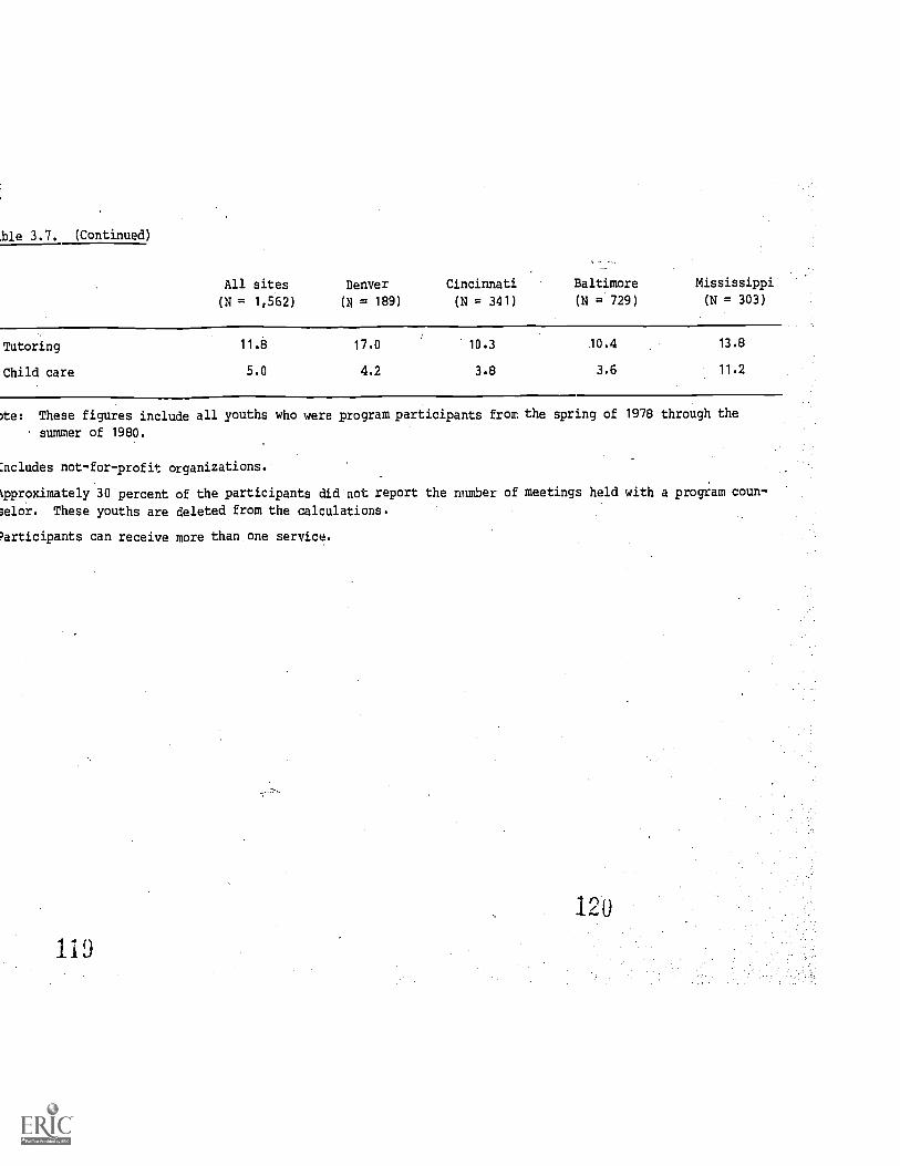
ble 3.7. (Continued)

-

All sites Denver Cincinnati Baltimore Mississippi

(N = 1,562) (N = 189) (N = 341) (N = 729) (N = 303)

Tutoring 11.8 17.0 10.3 10.4 13.8

Child care 5.0 4.2 3.8 3.6 11.2

xte: These figures include all youths who were program participants from the spring of 1978 through the

summer of 1980.

Cncludes not-for-profit organizations.

kpproximately 30 percent of the participants did not report the number of meetings held with a program coun-

;elor. These youths are deleted from the calculations.

?articipants can receive more than one service.

li9

A variety of services was provided to the YIEPP participants across

the sites, though no particular set of services was required. Differences

in services thus reflect individual program operator choice. On average,

youths met with a program counselor 1.8 times per month; this varied from a

high of 3.1 times .per month in Cincinnati to a low of 0.9 times per month

in Baltimore, which ran a very. large program. The, special program service

most often reported was an orientation meeting, mentioned by 66.5 percent

of the sample. The next most common service was employment counseling,

mentioned by 53.9 percent of the sample. The remaining services, from the

most to the least frequently reported, were educational or aptitude testing

(25.3 percent), reimbursement of transportation expenses (14.0 percent),

tutoring (11.8 percent), and child care (5.0 percent). Site profiles show

Denver concentrating on employment counseling, but also providing the

greatest amount of tutoring. Cincinnati offered the most employment

counseling, and also a relatively large amount of educational or aptitude

testing and transportation reimbursement. Baltimore offered fewer special

services (beyond orientation) than the other sites; Mississippi offered

transportation and child care services.

The Duration of Program Participation. Table 3.8 shows mean weeks

of program eligibility, mean weeks participating, and the percentage of

eligible time participating by youths who were ever program participants.

These youths were eligible for an average of 114.4 weeks, and participated

for 56.1 weeks, or 51.2 percent of this time. This (reasonably high)

percentage varied from 58.6 percent in Baltimore, to approximately 46

percent in Cincinnati and Mississippi, down to 40.6 percent in Denver.

These results further confirm our impression of the relative efficacy of

YIEPP implementation across these sites.

Table 3.9 decomposes these results by cohort, sex, and race.

Reading down the third column of this table we find the 15- to 16-year-old

cohort participated for a somewhat higher number of weeks but in propor-

tional terms it participated slightly less than the older cohort.- Males

participated slightly less than females. Across race'groups, blacks

participated the most, followed by Hispanics and whites. For joint race/

sex categories, black females showed the greatest,' and white males the

Table 3.8. Duration of Program Participation by Site, for Program Participants

Mean weeksprogram-aeligible

Means weeks bparticipating

Percentage ofeligible timeparticipating

All sites (N = 1,562) 114.4 56.1 51.2

Denver (N = 189) 121.1 47.8 40.6

Cincinnati (N =341) 116.7 50.4 46.3

Baltimore (N = 729) 114.4 64.6 58.6

Mississippi (N = 303) 107.5 47.0 45.3

Note: These figures include all youths who were ever p *Am participants,

from the spring of 1978 through the summer of 19i-,1.

-

aWeeks program-eligible equals total number of weeks in all seasons forwhich a youth was eligible to participate.

bWeeks participating equals total number of weeks employed in program jobs.

12265

Table 3.9. Duration of Program Participation by Cohort, Race and Sex,for Program Participants

Mean weeks Percentage of

program-a Mean weeksb

eligible time

eligible participating participating

Age in June 1978:

15-16 (N = 944)

17-20 (N = 618)

117.8

109.2

57.3

54.2

50.0

52.9

Male (N = 713) 116.3 54.9 49.1

Female (N = 849) 112.8 57.1 52.9

White (N = 65) 110.5 46.3 45.4

Black (N = 1,398) 114.2 56.7 51.8

Hispanic (N = 109) 119.6 54.2 47.0

White male (N = 32) 113,4 43.8 40.7

White female (N = 33) 107.7 48.7 49.9

Black male (N = 631) 115.9 55.3 49.6

Black female (N = 757) 112.7 57.8 53.6

Hispanic male (N = 50) 123.1 56.3 47.6

Hispanic female (N = 59) 116.6 52.4 46.6

Note: .These figures include youths from all four sites who were ever programparticipants, from the spring of 1978 through the summer of 1930.

aweeks program-eligible equals total number of weeks in all seasons fora youth was eligible to participate.

1,-,Jeks participating equals total number of tieks employed in program -;obs.

, ...... 1

least, YIEPP attachment: This is consistent with the relative ability of

these groups to find non-YIEPP employment. Of further interest is the

relatively strong program attachment of those white females who parti-

cipated at all. The low total participation rates for white females

reported in Tables 3.3 and 3.4 were due to low rates of initial partici-

pation. White females who did join the program showed strong attachment to

it.

These findings are refined by the regression-adjusted i,rates of

Table 3.10. With these adjustments, the site, cohort, and sex results are

essentially unchanged. However, the race and sex/race rates are consider-

ably altered when adjustment is made for differential site effects, par-

ticularly the low overall participation rate in Denver, where almost all

sample Hispanics reside, and the high overall participation rate in Balti-

more, that contains a plurality of the sample observations and is heavily

black. After adjustment Hispanics showed the strongest program attachment,

with blacks only slightly more attached than whites. The highest rates

were for male as well as female Hispanics, with the next highest rates for

black and white females. Next in order were black males, and finally white

males showed the least program attachment. These results differed from the

cumulative (ever joined) results of Table 3.4; after regreSsion adjustment,

blacks were more likely to join YIEPP, but Hispanics who joined remained

more attached to the program. Whites were particularly unlikely to join,

but once they did join, their attachment behavior was relatively similar to

that of the other groups.

Summary

YIEPP participation was quite high, varying from 68.8 percent of

eligibles in Baltimore, down to 38.8 percent of eligibles in Denver, for a

sample average of 56.2 percent. Intersite variation was consistent with

reports of the relative success of program imple%entation in these sites.

Rates for the 15- to 16-year-old-cohort (youths who aged through the

program) were higher, averaging 65.8 percent of eligibles. These higher

rates are an indication of what might be expected in an ongoing national

program. The experience over time of this young cohort also suggests that

participation peaked at ages 16 to 17 and dropped off thereafter. This is

consistent with the relative earnings opportunities of the entry level,

minimum wage jobs offered by the program.

Table 3.10. Ad'usted Duration of Pro am Partici ationby Site, Cohort, Race and Sex, for Program Participants

Percentage ofeligible timeparticipating

Denver

Cincinnati

Baltimore (reference group)

Mississippi

36.5**

46.9**

59.0

46.3**

Age in June 1978:

15-16 50.5

17-20 (reference group) 52.2

Male (reference group) 49.4

Female 52.7

White 49.0

Black (reference group) 50.6

Hispanic 59.8

White male 45.7

White female 52.2

Black male (reference group) 48.7

Black female 52.2**

Hispanic male 59.7**

Hispanic female 59.9

Note: The percentage of eligible time participating, for youths who wereever participants from the spring of 1978 through the summer of 1980,was estimated as a function of site, cohort, sex and race. Predictedpercentages for each characteristic are calculated at the overallsample mean values of the other characteristics. See Appendix Bfor parameter estimates and sample means.

**Percentages for these groups are signifipantly different from the per-centage for the reference group at the 5 percent significance level.

125 68

Females were slightly more likely than males to participate in

YIEPP. Blacks had the highest participation rates by a wide margin,

followed by Hispanics and then whites. The highest rates were for black

females, and the lowest were for white females. Race/sex participation

differentials can be explained largely by recourse to group differences

in the ability to find non-YIEPP employment.

Youths who were living with neither natural parent, married, or

had their own children were less likely to participate in YIEPP than the

rest of the sample. The effect was strongest for married youths. This

reinforces the finding that the entry level, minimum wage nature of program

employment made YIEPP most attractive to youths who were living at home,

and had not yet made the transition to adulthood.

In-school youths were more likely than dropouts to participate in

the program. Within each group, youths previously employed in the program

were very much more likely to participate in the current period. Also

within each group, not employed youths were more likely to participate than

were youths employed at a nonprogram job. These results are consistent

with the YIEPP school enrollment requirement, and the relative attractive-

ness of the program to youths who cannot otherwise find employment.

When the focus shifts to YIEPP participants, we find reasonable

stability of employment--only 15.4 percent of participants held more than

two YIEPP jobs. Fully 71 percent of these jobs were in the public sector,

with strongest private sector representation in Denver and the weakest

in Mississippi. Overall, participants spent 51.2 percent of their program-

eligible time employed on t. YIEPP job.

Among participants, program attachment was strongest for black

females and weakest for white males. Combined with previous results,

this finding means blacks were the most likely to join YIEPP, but Hispanics

who joined remained more attached to the program than any other group.

Whites were particularly'unlikely to join the program, but once they did

join, their attachment behavior was relatively similar to that of the other

groups.

CHAPTER 4

PROGRAM EFFECTS ON SCHOOL ENROLLMENT

These results suggest, however, that a successful policyto reduce unemployment among dropouts might well have theside effect of encouraging boys to drop out of schoolbefore high school graduation.

Duncan (1965;- p.134)

This quotation identifies a problem which has too often been

neglected by policies directed at the youth unemployment problem. Recent

studies support the notion that labor market interventions designed to

increase youth employment may have the undesirable side effect of de-

creasing school enrollment among youths from low income households.1

In

the context of a subsidized employment program, a potential solution is

to permit program participation only among youths who are enrolled in

school. This school enrollment requirement was one of the major innova-

tions of YIEPP.2

Measurement Issues

The potential school enrollment effects of YIEPP can be looked at

in two ways. First, the program can be regarded as an opportunity to

increase school enrollment within the target population, using program

jobs as the inducement. From this perspective, the program is successful

only if it exerts a significantly positive effect on school enrollment.

Second, the program can be regarded as one more subsidized youth employment

program, this time with an attempt to avoid negative school enrollment

effects. From the second perspective, the absence of such negative effects

is a' significant accomplishment. In this chapter we report on 'YIEPP's

success from each of the two perspectives.

1

See Ehrenberg andChapter 6 below.

2

Marcus (1982), Gustman and Steinmeier (1981), and

Such a requirement is,component of Job Corps'.

however, an operational part of the residential

71 127

Implementation Issues with Respect to Schooling. The YIEPP school-

ing requirement is usually described as "enrollment and satisfactory

performance in a program leading to a high school diploma or GED" without

reference to the implementation issues associated with local standards and

their enforcement. In this section we briefly review some of these issues

to provide a more realistic backdrop for the school enrollment effects

analysis of this chapter.1

Enforcement of schooling standards was a new task for the CETA

prime sponsors administering YIEPP. This task called for a good working

relationship with the local school administration and required much

effort. The demand for monthly school performance information was felt to

be particularly burdensome, 'even though, for their part, the schools were

asked only to monitor enrollment and performance; enforcement of standards

was the responsibility of YIEPP prime sponsor managers. While local

standards varied across sites, relatively uniform standards for the purpose

of program eligibility were negotiated by the fall of 1978. These typi-

cally called for a D grade average, and for a maximum number of unexcused

absences which varied from 4 to .5 to 20 or 25 days per semester. For YIEPP

participants enrolled in a GED program, the school requirement was typi-

cally the teacher's assessment of "satisfactory performance."2

As for actual, as opposed to desired, reporting of school atten-

dance and performance--data collection procedures began only after the fall

of 1978, and in some sites lagged until the fall of 1979. School atten-

dance data were, in general, collected monthly, but data on, grades were

collected on the basis of the school's reporting period. Since there were

delays in acting on negative individual school performance reports, atten-

dance problems were more often the cause of terminations than grade perfor-

mance problems. An even larger reason for termination was the relatively

large number of youths dropping out of school; 17 percent of all program

1The implementation information that follows is summarized from various

chapters in Diaz et al. (1982).

2The availability of GED programsvaried significantly across sites;'for

example, Baltimore had a strong GED program, whereas Mississippi initially

did not have one at all.

128 72

terminations were due to this factor. Participants were, however, gener-

ally terminated only after several intermediate steps--warning letters,

temporary suspension from YIEPP employment, and so forth.

Despite these difficulties, enforcement of the school enrollment

requirement appears to have been good, although, as suggested, school

enrollment requirements were more characteristically enforced than were

attendance and grade requirements. In a study conducted by MDRC, 21

percent of participants were found to be ineligible for YIEPP, but 85

percent of these case of ineligibility were due to the youths' failure to

meet the income tests. In addition, analysis of local field survey data

showed very few eligibles reporting YIEPP employment while not enrolled in

school. (See Chapter 3, Table 3.6.)

Finally, it must be kept in mind that the schools played important

roles in both recruitment and job placement under YIEPP. Outreach efforts---

were strong in the schools, recruiting large numbers of youths who were

already in school. Furthermore, public schools provided the greatest

number of jobs for the demonstration, a situation which tended to help

create ties between prime sponsors and local school administrators. In

sum, reasonable working relationships were usually developed with local

school systems, and these aided the reasonably careful enforcement of the

YIEPP enrollment requirement. At the implementation level, the program

model of a school-enrollment-constrained, guaranteed minimum wage job,

appears to have had a fair test.

Estimating Program Effects on School Enrollment. The main outcome

measures in this chapter are "enrolled in school or not" for the fall of

1978 and the fall of 1979. A youth was considered to be in school in a

particular fall if he or she reported in response to survey questions that

he or she was enrolled at any time from September through December.1

We

1 Because school enrollment is the social norm for youths in this agebracket, self-reported enrollment data could' overstate the true enrollmentrates. In the previous impact report, enrollment data from the surveywere compared with enrollment information obtained from the school recordssearch (Farkas et al. (1980)). Self-reportea enrollment rates were fourto five percentage points higher than rates calculated from school rec-ords, but this is not all response error. The school records did notreflect enrollment in alternative educational. programs. More important tothe estimation of program effects, both pilot'and comparison sites showedapproximately the same amount of disagreement between the two measures ofschool enrollment. Consequently, we discount the fact of self-reportedenrollment data as a source of bias in program effect estimates.

73

129

summarize these outcome measures as enrollment rates, i.e., the percentage

of the sample of youths who were enrolled.

The central methodological problem in measuring program effects on

school enrollment rates is to estimate what the school enrollment rate in

the pilot sites would have been in the absence of YIEPP. In particular, if

the comparison site school enrollment rates are to represent the pilot site

rates in the absence of YIEPP, the actual comparison site rates must be

adjusted to reflect the demographic characteristics and preprogram school-

ing experiences of pilot site youths. With this adjusted estimate in hand,

-the program effect is simply the difference between the pilot site enroll-

ment rate actually observed and the estimated rate in the absence of the

program.

The following procedure was used to adjust the comparison site

enrollment rates. For each fall a multivariate model of enrollment was

estimated using a sample of youths eligible for the program in that period

from the pilot and comparison sites1 Program eligibility was defined by

age and graduation status, exactly as in Chapter 3. Included in the model

as right hand side variables were a dichotomous variable indicating whether

a youth was from a pilot or comparison site, dichotomous variables repre-

senting race and sex groups, age in months, school enrollment status in

the fall of 1977, and highest grade completed as of the summer of 1977.

The coefficients in this model estimate the independent effect of the right

hand side variables on the probability that a youth is enrolled in.school. ,

Using the estimated coefficients, an enrollment, rate was predicted,

assuming that youths were not in a pilot site but had the average demo-

graphic characteristics and preprogram schooling experiences of the pilot

site sample .2 This adjusted comparison site enrollment rate is the

estimate of what enrollment rates in the pilot sites would have been in the

absence of the program.

1Because the dependent variable in the model, enrolled or not, is dicho-

tomous, probit models were estimated.

2Coe ficient estimates from the enrollment models and the pilot site means

for the demographic and preprogram variables can be found in Appendix B4.

130 74

The remainder of this chapter is organized as follows. The next

section reports program effects on total school enrollment and enrollment

by type of program (programs leading to a regular high school diploma or

the GED). The third section presents the estimated program effects on

school enrollment for the 15- to 16 -year -old cohort. This is followed by

an examination of program effects by site and by race and sex subgroups of

the population. The, final section summarizes the key findings of the

.chapter.

Program Effects on School Enrollment by Type of Degree Program

As a guide to understanding the educational context in which YIEPP

operated, Table 4.1 displays unadjusted school enrollment rates, separately

for pilot and control sites, for the preprogram and during-program periods.

In the fall of 1977, over 80 percent of the youths in the sample were

enrolled in school, and almost all of the enrolled youths were in a program

leading to a regular high school diploma rather than the GED.1

As the

youths age, enrollment rates drop. Two years later, in the fall of 1979,

enrollment rates for program-eligible youths had fallen to the 50 to 60

percent range. Also as the youths age, GED enrollment becomes a signifiT

cantly higher fraction of total enrollment.

How do these enrollment rates, for the YIEPP sample compare with

national enrollment rates for 16- to 19-year-old youths in the United

States? As described in Chapter 2, youths in the YIEPP sample are not

typical of high school age youths in general. To remove the gross incom-

parabilities, school enrollment rates during October, 1978, for YIEPP

sample youths and for all United States youths were calculated separately

for age, race and sex groups. These rates are shown in Appendix A, Table

A4.1. Holding age, race, and sex constant, youths in the YIEPP sample had

substantially lower enrollment rates than the averages for all youths in

the United States. The differences are greatest for white males and white

females and smallest for Hispanic youths.

1 Enrollment rates in GED and regular high school programs may not sum to

the total enrollment rate because youths can be enrolled in both types of

programs during the same fall.

75

Table 4.1. School Enrollment Rates by Type of Degree Programand Pilot or Control Sites

Preprogram During=programFall 1977 Fall 1978 Fall 1979

Total school enrollment:

Pilot sites 84.2 73.8 61.3

Control sites 80.9 66.0 56.7

Regular school enrollment:P.

Pilot sites 80.9 68.3 55.2


GED enrollment: b

Pilot sites 3.3 5.7 6.2


Sample sizes:c

Pilot sites 2,778 2,652 2,107

Control sites 1,255 1,188 930

aEnrolled at all in a program leading to a regular high school diploma.

bEnrolled at all in a program preparing students for the GED examination.

cThe sample includes youths who have completed three waves of the localfield survey and are eligible for the program during the period inquestion. See Chapter 2 for further details.

76

Estimates of YIEPP's effect on the school enrollment rates of

program-eligible youths are shown in Table 4.2.

In_ the fall of 1978 YIEPP is estimated to have increased total

school enrollment by 4.8 percentage points from an enrollment rate of 69

percent in the absence of the program. This finding is statistically

significant at the 1 percent level. It is also very similar to the esti-

mated program effect reported in the previous volume on program impactg.1

The effect on total enrollment was due to almost equal increases in enroll-

ment among youths in regular high school and GED programs. In the fall of

1979, the estimated program effect drops from 4.8 to 2.5 percentage

points. This drop is primarily composed of a decline in the program effect

on regular school enrollment, which goes from 2.9 percentage points in 1978

to 0.9 percentage points in 1979. The program effect on GED enrollment in

the fall of 1979 drops less dramatically from the 1978 result. (The

reasons for this decline in the estimated regular school enrollment effects

(and its components--the dropout and return-to-school rates) are discussed

on pages 81 -32 below.)

Tests for Attrition Bias. An additional potential source of e:'or

in measuring program effects from panel data is sample attrition trk

the pilot/comparison site research design used in this study, the to W:: Of

original sample members to follow-up surveys introduces bias into the

measurement of schooling effects when the average enrollment rates of these

individuals differ between the pilot and comparison sites. In the previous

impact report, statistical tests for sample selection bias in.-the school

enrollment effects were performed. These tests found that attrition bias

was not a problem.2 In this report program effects on total school

enrollment rates have been estimated for a special attrition sample of

1 The previous finding was a program effect of 4.8 percentage points addedto the enrollment rate of 70.4 percent in the absence of the program(Markas et al. 1980). The small differences between the findings aredue to differences in the samples and statistical methodology used.

2The results are reported in Farkas et al. (1980). The discussion there

also includes a more detailed discussion of the relationship between sam-

ple attrition and the bias it can introduce into the measurement of

program effects.

77 133

Table 4.2. Program Effects on School 'Enrollment Rates

by Type of Degree Program

Estimated


rate in the percent of rate

Sample Pilot site absence of

the program

Progrl in the absence of

size rate effect the program

Total school enrollment:

Fall 1978

Fall 1979

3,840

3,037

73.8

61.3

69.0

58.8

Regular school enrollment:

Fall 1978 3,840 68.3 65.4

Fall 1979 3,037 55.2 54.3

, .

GED enrollment:

Fall 1978 3,840 5.7 3.3

Fall 1979 3,037 6.2 4,5

4.8*** 7.0

2.5* 4.3

2.9** 4,4

0.9 1.7,

2.4***

1,7**

72.7

37.8

a

The sample includes youths who have completed three waves of the local field survey and are eligible

for the program during the period in question. See Chapter 2 for further details,

bThis is a regression-adjusted comparison site mean, fit at pilot site average personal characteristics

and preprogram school enrollment. Means of the right hand side variables and probit coefficient esti-

mates are reported in Appendix B.

This is the 'difference' between columns 2 and 3, with statistical significance computed from the

t-statistic on the pilot site dummy variable regression coefficient.

significant at the 10 percent level.

** . significant at the 5 percent level,


Hispanic youths in Denver/Phoenix and black youths in Baltimore/Cleveland

who did not respond to the Wave II survey but who were reinterviewed at a

later date. School enrollment effect estimates for these and matching

youths who completed all three survey waves are reported in Appendix C;

Table C2.2.

For Hispanic youths in Denver, the program effects in the attrition

sample are lower than the effects estimated for the analysis sample in the

fall of 1978 and higher than those in the fall of 1979. But the differences

are small in magnitude, and insignificantly different from zero. In

Baltimore, the program effects on the school enrollment rates of black

youths in the attrition sample are much larger than the program effects

estimated for the analysis sample. But, because of the small size of the

attrition sample, the difference between the program effects is not statis-

tically significant. When the program effects for the two samples are

combined in a weighted average based upon the attrition rates, this summary

measure of program impacts is twice 'as large as the estimates from the

analysis sample alone -- suggesting that, in Baltimore at least, estimated

program effects based upon the analysis sample may underestimate the true

program effect.

Effects on Dropout and Return-to-School Rates. The discussion

above focuses on a-key reason as to why the program effect declined in the

second year. To answer this question further and understand more about the

way YIEPP acts to increase the schooling activity of eligible youths, we

now ask how the.program affected the probability of school enrollment for

youth who were and were not previously enrolled in school. Participation

in YIEPP was an option for all eligible youths, regardless of their pre-

vious school enrollment status. For youths who were previously in school,

the program can increase school enrollment rates by reducing the number of

dropouts. For youths who were previously out of school, the program can

increase school enrollment rates by increasing the probability that these

youths return to school.

Table 4.3 displays c.stimated program effects on dropout and return-

_to-school rates. The dropout rate is defined as the percentage of youths

enrolled in the previous fall who were not enrolled in school in the fall a

Table 4.3. Program Effects on Dropout and Return-to-School Rates

Estimated

pilot site Program as

rate in the percent of late

Sample Pilot site absence of Program in the absence of

size rate the program effect the program

ropout rates:a

Fall 1978 3228 16.8 21.2 -4.4*** -20.8

Fall 1979 2215 23.6 23.3 0.3 1.3

eturn -to -school rates:b

Fall 1978 612 18.7 12.1 6.6** 54.5

Fall 1979 822 15.3 13.9 1.4 10.1

See notes a, b, and c to Table 4.2 for definitions of the sample, the estimated pilot site rate in the

absence of the program, and the program effect as percent of rate in the absence of the program:

Of youths who were enrolled in the preceding fall, the percentage currently not enrolled.

Of youths who were not enrolled in the preceding fall, the percentage currently enrolled.

** = significant at the 5 percent level.


138

year later. For example, a dropout in the fall of 1979 is a youth who was

enrolled in the fall of 1978 but not enrolled in 1979. The return-to-

school rate is defined as the percentage of youths not enrolled in the

previous fall who were enrolled in school the next fall.

Looking first at the fall of 1978, the average dropout rate in the

pilot sites was 16.8 percent. This rate is estimated to have been de-

creased by 4.4 percentage points as a result of the operation of YIEPP.

Also in the fall of 1978, the program increased the return-to-school rate

in the pilot sites by 6.6 percentage points from the 12.1 percent expected

in the absence of the program. Both effects are statistically significant.

Thus, YIEPP had a positive influence on the enrollment rates both by

keeping in school youths who were previously enrolled (that is, by reducing

the dropout rate) and by inducing youths who were previously out of school

to return to an educational program. Note that, although the program

effects on dropout and return-to-school behavior are of similar magnitudes,

the largest contribution to increased enrollment in the fall of 1978 comes

from the reduction in the dropout rate. This follows from the fact that

most of the youths in the sample were enrolled in the fall of 1977 and

therefore subject only to program effects on the dropout rate.1

Program effects on dropout and return-to-school behavior disappear

in the fall of 1979. YIEPP is estimated to increase, rather than reduce,

dropout rates in 1979, although this estimate is not significantly differ-

ent from zero. And, although the proaram is still estimated to increase

the rate of return-to-school activity, this finding, also, is not statis-

tically Significant.

How can YIEPP have essentially no effect on dropout and return-to-

school behavior in the fall of 1979 and still show a positive effect on

total school enrollment? The answer lies in the conceptual differences

between the enrollment, dropout, and return-to-school rates and the age

composition of the sample as it changes over time. The dropout and return-

1A similar finding was reported in the previous impact report (Farkas etal. 1980).

to-school measures for the fall of 1979 take as given the observed enroll-

ment rates in the fall of 1978. For example, the dropout rate in the fall

of 1979 is calculated from the sample of all youths enrolled in the fall of

1978, regardless of whether their enrollment was due to the program or not.

This means that the program effects on the dropout and return-to-school

rates in the fall of 1979 represent the incremental change in school

enrollment from 1978 to 1979. As reported in Table 4.3, this change was

small. But enrollment in the fall of 1979 is also affected by what the

program did to enrollment in the previous fall. This is because, on

average, youths enrolled in one period are more likely than youths not

enrolled to be in school in the following period. Therefore, the program

effect on total school enrollment in the fall of 1979 is less than that in

the fall of 1978 because of a decline in the effect on dropout and return-

to-school behavior, but it is greater than zero because of the lagged

effects produced by YIEPP-induced increases in enrollment in the fall of

1978.

Why do the estimated program effects on the dropout and return-to-

school rates decline from 1978 to 1979? As noted above, part of the answer

lies in the nature of the YIEPP analysis sample. To produce incremental

enrollment gains in the fall of 1979 the program must have enlisted

new program participants during the preceding year. This is particularly

clear in the case of return-to-school rates. By definition, the program

effect on return-to-school rates is generated by increasing the school

enrollment of previously out-of-school youths, or by drawing new partici-

pants from this population. But the potential for obtaining new partici-

pants in 1979 is more limited among the youths in the analysis sample than

among the actual youth population eligible for YIEPP. ;. because the

analysis sample contains proportionately fewer youths who could age into

program eligibility from the fall of 1978 to the fall of 1979 than were in

the eligible population. In other words, the analysis sample contains

proportionately fewer youths who were 16 years ola in 1979 than the actual

eligible population in the pilot sites. It is these youths, as shown in

Chapter 3, who were most likely to participate in YIEPP.

82

This argument about the relationship between the estimated school

enrollment effects and the age composition of the analysis sample is

confirmed by the findings on dropout and return -to-school rates for the

15- to 16-year-old cohort to be presented in the next section. This cohort.

includes all the youths in the sample who are not initially eligible, but

who can age into the program sometime after its start-up. Program effects

on enrollment rates for this cohort are only slightly smaller in the fall

of 1979 than in the fall of 1978, and there is a significant effect on

return-to-school rates in 1979. These results suggest that at least part

of the explanation for the estimated decline in program effects on school

enrollment is the age structure of the analysis sample.

Enrollment by Type of School and Curriculum. Table 4.4 shows the

type of school and curriculum chosen by enrolled youths in the pilot and

control sites during the program. Over 90 percent of students were enroll-

ed in public schools in both the pilot and control sites. The remainder

attended private or special-purpose schools with either private or public

support. In both the fall of 1978 and the fall of 1979, the major differ-

ence in enrollment patterns between the pilot and comparison sites is in

the percent of students in alternative education either operated by the.

public schools or by community-based organizations. Most of these prograMs

prepare students for the GED exam. This difference is consistent withthe

previous finding that YIEPP effects on enrollment in GED programs contrib-

ute a significant proportion of the overall program effect on school

enrollment. In terms of the type of education program, 70 percent of the

students in the sample were enrolled in general studies programs with

another 15 to 17 percent participating in vocational or technical training

programs. Pilot site youths favor commercial and vocational programs over

the general studies or college preparatory programs, but those pilot/com-

parison site differences are relatively small.

Program Effects on School Enrollment for the 15- to 16-year-old Cohort

The 15- to 16-year-old cohort is of special interest in the assess-

ment of program effects. It consists of youths who age into program

eligibility when they turn 16, the earliest age at which youths can parti-

cipate in YIEPP. These youths provide the best estimates of what would

83

1_ 4 1

Table 4.4. Enrollment Characteristics by Pilot or Control Site

Fall 1978 Fall 1979

Pilotsites

(N=1,739)

Controlsites(N=592)

Pilotsites(N=872)

Controlsites(N=406)

Type of school (%):

Public school--regularcurriculum. 84.1 89.2 80.4 86.9

Public school--alternativecurriculum 11.2 8.6 13.6 9.7

Private/parochial school 1.7 1.2 1.8 1.2

Special school for handicapped 1.2 0.5 0.3 0.7

Community-based school orstreet academy 1.8 0.5 3.9 1.5

Type of program (%):":"

General studies 70.2 70.3 70.5 72.0

College preparatory 5.8 9.3 4.9 7.1

Commerical or business 5.7 4.8 5.6 3.9

Vocational or technical 17.0 14.5 14.6 14.4

Agricultural 0.1 0.3 0.3 0.2

Othera 1.2 0.8 4.1 2.4

Note: The sample includes enrolled program-eligible youths who respondedto the survey questions.

aThis category includes all other programs.

84

have happened to cohorts. of youths as they aged through the period of

eligibility for the program and the best indication, of what would happen in

an on-going national program. In contrast, the full analysis sample

includes youths who could only begin their program participation at age 17

or later because the program had just started. In an ongoing program, the

older cohort would have had the opportunity to participate at an earlier

age; therefore, the program effect on school enrollment at ages 17 through

19 could be different from that observed here. While one or two years of

difference in age may not be important in an older population, the rapid

changes youths experience in school and work activities as they move from

16 to 19 years make the distinction important for this age group.

Table 4.5 reports the estimated program effects on enrollment,

dropout and return-to-school rates for the 15- to 16-year-old cohort. In

the fall of 1978 about 38 percent oGthe younger youths in the pilot sites

were enrolled in a regular degree or GED program. Out of this 88 percent,

about 4 perCentage points are estimated to have resulted from the operation

of YIEPP in the pilot sites, a program effect that is similar to the effect

estimated for all youttis4 in the analysis sample. This increase in total

school enrollment con6':41.:s of both an estimated reduction in the dropout

rate and an increase th :ceturn-to-school rates. In comparison to the total

sample, the program has about the same proportionate effect on dropout

rates for the 15- to 16-year-old cohort in the fall of 1978. But YIEPP has

a much larger effect on return-to-school behavior, again in proportion to

the estimated rates in the absence of the program, for the younger cohort

than for the full' sample. Fewer members of the 15- to 16-eyear-old cohort

were already out of school in the fall of 1977; and, because they were 14

to 15 years of age at the time, these youths had probably only recently

just dropped out of school. The larger return-to-school effects for the

15- to 16-year-old cohort is consistent with the hypothesis that partici-

pation in YIEPP, and re-enrollment, is more attractive to younger persons

who have only recently left school.

As noted in the previous section, the estimated program effect on

total school enrollment for the 15- to 16-year-old cohort does not decline

as rapidly from the fall of 1978 to the fall of 1979 as it does for the

85

Table 4.5. Program Effects on Enrollment, Dropout and

Return-to-School Rates for the 15- to 16-year-old Cohort

Estimated

pilot site Program effect asPilot rate in the ,a percent of rate

Sample site absence of Program in the absence ofsize rate the program effect the program

tal school enrollment rates:

Fall 1978 2,005 88.2 84.1 4.1*** 4.9

Fall 1979 1,920 75.7 72.4 3.3* 4.6

Dpout rates:

Fall 1978 1,924 9.6 12.9 -3.3** -25.6

Fall 1979 1,544 17.3 16.8 U.5 3.0

:urn-to-school rates:

Fall 1978 81 34.4 8.6 25.8*** 3UU.0

Fall 1979 276 27.3 16.1 11.2** 69.6

iulative dropout rate:

Fall 1979 1,920 24.3 27.6 -3.3* -12.0

notes to Tables 4.2 and 4.3. The sample is restricted to youths who were 15 or 16 in June, 1978.

= significant at the 10 percent level.



sample as a whole. Unlike estimates for the full sample, there is a

positive and significant effect on this younger cohort's return-to-school

rate in 1979.1 Additionally, while the program effect on the dropout

rate in the fall of 1979 is about zero, which is similar to the finding for

the full sample, YIEPP had, by the fall Of 1979, reduced the cumulative

dropout rate of this younger group. As seen in the bottom panel of Table

4.5, the cumulative,drop-out rate decreased from an estimated 27.6 percent

in the absence of the program to 24.3 percent: a 12 percent reduction.

In summary, the major difference between program effects on the

schooling behavior of the 15- to 16-year-old cohort and on the behavior of

the full analysis sample is the larger effects on the retuxn-to-school

rates of the young cohort. Thus, YIEPP, for this cohort, has an important

impact on drawing younger teenagers back into school, a major objective of

YIEPP.

Cumulative Effects: A Longitudinal Perspective. Because the 15-

to 16-year-old cohort most closely represents the experiences of a typical

cohort aging through an on-going national program, examining program

effects on school enrollment in a longitudinal perspe-ctive is particularly

appropriate. In Table 4.6 program effects on total school enrollment in

the fall.of 1978 and the fall of 1979 are considered jointly.2

The first panel of the table presents estimated program effects for

youths who were enrolled in the preprogram period, Fall 1977. This group

comprises over 95 percent of the 15- to 16-year-old cohort. Let us first

1A program effect on return-to-school rates in the fall of 1979 depends

on the recruitment of new program participants in the preceding year.

But, due to operational difficulties, the Denver program was not allowed

to enroll new participants after March, 1979. To check the impact this

might have on estimated school enrollment effects, Table 4.5 was re-

estimated excluding youths in the Denver and Phoenix sites. (The results

are presented in Appendix A, Table A4.4.) The estimated program effect on

return-to-school rates in the fall of 1979 rises to 12.5 percentage

points.

2The sample used in estimating the results for this table includes youths

in the 15- to 16-year-old cohort who were eligible for YIEPP in both the

fall of 1978 and the fall of 1979. Program effects on enrollment rates

in the fall of 1978 And the fall of 1979 are estimated jointly in a

bivariate probit model in which the covariance parameter is allowed to

vary between pilot and comparison sites.

14687

Table 4.6. Cumulative Program Effects on School Enrollment Ratesfor the 15- to 16-year-old Cohort

Estimated pilot Program effect as

Enrollment status Pilot site rate in the percent of rate in

in Fall 1978 and sitea

absencebof the PrograE the abSence of the

Fall 1979 rate program effect program

For youths enrolled in school,Fall 1977 (N=1,766):

Enrolled Fall 1978 andnot enrolled Fall 1979

Not enrolled Fall 1978and enrolled Fall 1979

Enrolled Fall-1978 andenrolled Fall 1979

For youths not enrolledin school, Fall 1977(N=79):

Enrolled Fall 1978 andnot enrolled Fall 1979

Not enrolled Fall 1978and enrolled Fall 1979

Enrolled Fall 1978 andenrolled Fall 1979

Cumulative return-to-school rate, Fall 1979(N=79):.

15.2 13.9 1.3** 9.4

3.3 2.4 0.9* 37.5

74.2 71.6 2.6** 3.6

15.2 11.9** 360.6

3.2 Ilu./ -8.5 -72.6

18.4 1.7 16.7 982.3

23.2 14.2 9.0 63.4

Note: The sample is restricted to youths who were 15 or 16 in June, 1978 and who were program-eligiblein both Fall 1978 and Fall 1979.

aTaken from the cross-tabulation of enrolled Fall 1978 by enrolled Fall 1979 for the pilot sites. See

Table A4.5 of Appendix A for the full set of results.bTaken from the adjusted comparison site cross-tabulation, fit at pilot site average personal character-istics (also found in, Table A4.5 of Appendix A).

cDifference between columns 1 and 2. Statistical significance has been approximately determined from th!!t-statistics of the parameters in the adjustment model measuring pilot-comparison site differences;

* = significant at the 10 percent level.** = significant at the 5 percent level.*** = significant at the 1 percent level.

14788

consider estimated pilot site rates in the absence of the program. Without

YIEPP, an estimated 14 percent of these youths would have stayed enrolled

in school for one more year and then dropped out by the fall of 1979. An

additional 2 percent would have been out of school in the fall of 1978

but would return to school in the fall of 1979. By far the largest percen-

tage of the youths would have continued to be enrolled through the two year

period. Finally, the, remainder of the group, less than 10 percent, would

have dropped out of school in the fall of 1978 and remained out in the

following year. (This residual category is not listed in Table 4.6.)

The program is estimated to have had positive and statistically

significant effects on all three enrollment patterns shown in the table.

It increased the percentage of youths who were enrolled in both falls by

2.6 percentage points, while it increased the percentage of the group

enrolled, in just one of the falls by 2.2 percentage points (1.3 + 0.9 =

2.2). These longitudinal results can also be summarized in a different

way: For the two complete school years during the operation of YIEPP,

pilot site youths in the 15- to 16-year-old cohort were enrolled an

average of 1.7 years, as measured by enrollment. status in the fall.1

It is estimated that, in the absence of the program, these youths would

have been enrolled an average of 1.6 years. The cumulative program effect

over the two years is 0.1 years, then, or an additional year- of school

enrollment for every 10 program-eligible youths.

Turning to the small group of youths who were not enrolled in the

fall of 1977, note that enrollment rates in the absence of-the program were

much lower for these youths. Most of the youths were not enrolled in

either the fall of 1978 or the fall of 1979. The only statistically

significant finding is a positive program effect on the, percentage of

youths who returned to school in the fall of 1978 and then dropped out

again by the fall of 1979. In terms of program effects on the cumulative

number of years enrolled, pilot site youths in this group were observed to

be enrolled an average of 0.6 years over the two year period. In the

1This average is calculated as follows. There were 7.3 percent youths

who were never enrolled, 18.5 percent who were enrolled in one fall, and

74.2 percent who were enrolled in both 1978 and 1979, for 'a weighted

average of 1.7 falls of enrollment.

-

absence of the program, the average number of years enrolled was estimated

to be 0.2 years, implying a program-induced increase of 0.4 years. This

larger effect for youths who were out of school in the preprogram period is

probably not statistically significant, but it does agree with the propor-

tionately large return-to-school effects already reported.

Finally, the bottom panel of Table 4.6 presents the cumulative

program effect on the return-to-school rate of youths who were dropouts in

the fall of 1977. In the absence of the program, over the two-year period

only 9 percent of these youths would have returned to school. YIEPP raised

this rate to 14.2 percent, an increase of about 63 percent. This differ-

ence, however, is not significant.

Program Effects on School Enrollment by Site, Race and Sex

Average program effects can mask considerable diversity. In this

section, program effect estimates are presented for the key subgroups

of the.eligible population. The methods for measuring program effects

remain the same, but attention is restricted to subsamples defined by

site, race, or sex.

--Effects by Site. Even with a relatively uniform program model,

differences across the sites in program operations and in the general

educational climate suggest that YIEPP's effects on school enrollment will

vary among the four sites studied. Table 4.7 presents the estimated

program effects on total school enrollment separately by site. In Denver,

positive program effects are observed, but they are small in magnitude and

insignificantly different from zero. Small program effects on school

enrollment in Denver are:consistent with the lower program participation

rates in this site, as described in Chapter 3.

The largest program effects are thcse estimated for Cincinnati, but

these estimates must be interpreted with caution, because corollary evi-

dence suggests that the reported findings for the Cincinnati site are

probably overestimates of theL-true program effect. First, program parti-

cipation rates in Cincinnati were average compared to the other sites.

While the correspondence is not likely to be exact, one would expect higher

school enrollment effects to be associated with higher program participa-

tion rates. Second, the Cincinnati school enrollment effect is at least

14990.

Table 4,7. Program Effects on Total School Enroll'ilint Rates by Site

Estimat



Sample Pilot site absence 'of Program in the absence of

size rate the program effect the program

/Denver:

Fall 1978 654 67.4 67.0 0.4 0.6

Fall 1979 506 52.4 50,7 1.7 3.4

1.1.1...

Cincinnati:

Fall 1978 1,085 72.6 64.5 8.1*** 12,6

Fall 1979 881 62.9 56.0 6.9*** 12.3

Baltimore:kLI

Fall 1978 1,299 74.8 71.9 3.9* 5.5

Fall 1979 1,037 64.2 61.8 2.4 3.9

Mississippi:

Fall 1978 802 79.3 75.5 3.8* 5.0 .

Fall 1979 613 62.0 64.7 -2.7 -4.2

All sites but Denver:

Fall 1978 3,186 75.2 69.6 5,6*** 8.0

Fall 1979 2,531 63.3 60.6 2.7* 4.5

See notes to Table 4.2.

15U

* = significant at the 10 percent level.

*** . significant at the 1 percent level.

partly due to an inexplicably rapid decline in the school enrollment rates

for Cincinnati's comparison site, Louisville. From the preprogram period

in the fall of 1977 to the fall of 1978, school enrollment rates for

eligible youths in Cincinnati declined by less than 10 percentage points

while the rates in Louisville declined by almost 2D percentage point$:. The

size of the enrollment decline in Louisville is larger than in any ,of the

other comparison sites, and it may be related to changing educational

conditions in the Louisville public schools, particularly the implementa-

tion of busing for racial integration. Over the period from 1977 to 1981,

total enrollments in the Louisville public schools fell by 16.4 percent,

while enrollments fell only 9.3 percent in the Cincinnati public schools.1

The estimated school enrollment effects in Baltimore and Missis-

.sippi are similar to each other and to the summary findings presented in

the last section. In the fall of 1978 the school enrollment rates were

about four percentage points higher as a result of the operation of YIEPP

in these sites, but they were lower for the second year of the program.

Effects by Race and Sex. Table 4.8 displays program effects on

enrollment, dropout and return-to-school rates separately by the race of

eligible youths. Black youths have estimated program effects that are

similar to the summary effects for the whole sample, which is not surpris-

ing--they constitute over three-quarters of the analysis sample. On the

other hand, white youths are estimated to experience relatively large,

positive effects on school enrollment, and the reported school enrollment

effects for Hispanic youths are estimated as essentially zero. Both of

these sets of findings have to be interpreted carefully. Most of the white

youths in the comparison sites sample, for instance, live in Louisville.

Whatever is depressing the school enrollment rates in Louisville, there-

fore, disproportionately affects the estimates of school enrollment effects

for white youths. Analogously, almost all of the Hispanic youths in the

1

These enrollment numbers are taken from an unpublished MDRC report on theconditions in the public school environments of the urban sites in theYIEPP analysis sample.

Table 4.8. Program Effects'on Enrollment, Dropout and

Return-to-school Rates by Race

Sample Pilot site

size rate

Estimated

pilot site

rate in the

absence of

the program

Program effect as

percent of rate

Program in the absence of

effect the program

Total school enrollment rates:

White:

Fall 1978 525 56.9 46.9 10.0*** 21.3

Fall 1979 407 43.1 28.4 14.7*** 51.8

Black:

Fall 1978 2,917 78.1 73.9 4.2*** 5.7

Fall 1979 2,313 66.2 65.7 0.5 0.8

Hispanic:

Fall 1978,,,

f.,t, 59.8 57.8 2.0 3.5

ko

wFall 1979 11/ 44.0 45.9 -1.9 -4.1

Dropout rates:

White:

Fall 1978 362 23.2 38.5 -15.3*** -39.7

Fall 1979 211 32.9 42.7 -9.8* -23.0

Black:

Fall 1978 2,564 14.7 18.2 -3.5** -19.2

Fall 1979 1,814 21.1 20.4 0.7 3.4

Hispanic:

Fall 1978 302 28.1 26.2 1.8 6.9

Fall 1979 190 38.0 29.8 7.8 26.2

153


Estimated

pilot site Program effect asrate in the percent of rate.

Sample Pilot site absence of Program in the absence ofsize rate the program effect the program

turn-to-school rates:

White:

Fall 1978 163 8.9 10.3 -1.4 -13.6

Fall 1979 196 8.7 2.7 6.0** 222.2

Black:

Fall 1978 353 22.2 12.8 9.4** 73.4

Fall 1979 499 17.0 19.1 -2.1 11.0

Hispanic:

Fall 1978 96 18.6 6.7 11.9** 177.6

Fall 1979 127 15.0 11.6 3.4 29.3

*

i*

notes to Tables 4.2 and 4.3.




156

sample live in Denver and Phoenix. It is therefore difficult to disen-

tangle a purely Hispanic difference in program effects from the operational

problems of the Denver site.

The bottom two panels of Table 4.8 show that the positive program

effect on the school enrollment of blacks in the fall of 1978 occurs as a

result of both a program-induced reduction in the dropout rate and an

increase in the propensity to return to school. In proportionate terms,

the return-to-school effect is larger, but it operates on just over 10

percent of the sample. Therefore, the largest contribution to the school

enrollment effect comes from the program's success in keeping eligible

youths in school. As with the summary findings, the incremental effects on

school enrollment, represented by the impacts on dropout and return-to-

school behavior in the fall of 1979, are insignificantly different from

zero.

Table 4.9 presents separate program effects on enrollment, dropout

and return-to-school rates for males and females. In the fall of 1978,

total school enrollment in the pilot sites was approximately the same for

both sexes, with the program contributing between four and five percentage

points to the enrollment levels for both males and females. These effects

on school enrollment rates were the result of program effects on both

dropout and return-to-school behavior; however, the return-to-school effect

for males is not significantly different from zero.

While program effects on males and females were similar in the fall

of 1978, there were important differences for 1979. The most striking

difference is that the estimated program effect for females in this period

is both relatively large and statisticalay signiiicant, while the effect

for males is essentially not different from zero. Thus, the overall

program effect on total school enrollment in the fall of 1979--2.5 percen-

tage points (Table 4.2)--is the weighted average of a small negative effect

for males and a large positive effect for females. The higher school

,enrollment effect for female youths in the fall of 1979 is, in part, due to

the fact that YIEPP is estimated to have significantly decreaSed the

dropout rates of females in this period while increasing the dropout rates

of males.1 Unlike some of the other differences in estimated program

1 It seems unlikely that the program actually induced male youths to drop

out of school in the fall of 1979. With reasonably careful enforcement

95 157

Table 4.9. Program Effects on Enrollment, Dropout and

Return-to-School Rates by Sex

Estimated


rate in the percent 'of rate

Sample Pilot site absence of Program in the absence of

size rate the program effect the program .

Dtal school enrollment rates:

Male:

Fall 1978 1,776 ' 73.1 68.7 4.4** 6.4

Fall 1979 1,463 59.0 60.4 -1.4 -2.3

Female:

Fall 1978 2,064 74.5 69.2 5.3*** 7.7

Fall 1979 1,574 63.6 57.3 6.3*** 11.0

copout rates:

Male:

Fall 1978 1,534 18.7 23.2 -4.5** -19.4

Fall 1979 1,068 25.6 20.9 4.7** 22.5

Yemale:

Fall 1978 1,694 15.0 19.3 -4.3** -22.3

Fall 1979 1,147 21.7 25.7 -4.0* -15.6


Estimated



Sample Pilot site absence of Program in the absence -of

;size rate the program effect the program

turn-to-school rates:

Male:

a

Fall 1978 242 16.0 12.6 3.4 27.0

Fall 1979 395 13.1 13.9 -0.8 -5.8

Female:

Fall 1978 370 20.5 11.7 8.8** 75.2

Fall 1979 427 17.4 14. 1 3.3 23.4

e notes to Tables 4.2 and 4.3.

* = significant at the 10 percent level.



161

1GU

effects across subgroups of the eligible youth population, this difference

in program effects on dropout rates for males and females cannot be ex-

plained by the composition of the sample. The male and female subgroups

are similarly distributed across the sites and age groups. This differ-

ence, therefore, must be related to sex differences in the attachment-to

school and work activity.

Summary

The schooling aspects of YIEPP may be judged minimally successful

if the school requirement simply prevented negative school enrollment

resulting from the increased employment of eligibles. A more socially

valuable program achievement would be a significant positive effect on

school enrollment and performance. We find that, overall, both of these

objectives were met on a modest scale.

Effects on Total Enrollment. With respect to total enrollment for

the sample as a whole, YIEPP produced modest but statistically significant

program effects. YIEPP increased school enrollment by 4.8 percentage

points in the fall of 1978, and by 2.5 percentage points in the fall of

1979. These effects are, respectively, 7.0 and 4.3 percent of the school

enrollment rates expected in the absence of the program..

Regular school enrollment increased by 2.9 percentage points during

the fall of 1978, and by 0.9 percentage points during the fall of 1979.

GED enrollment increased by 2.4 percentage points during the fall of 1978,

and by 1.7 percentage points during the fall of 1979. These findings

suggest that alternative educational programs (programs leading to a GED)

played an important role in the overall YIEPP school enrollment effect.

The school enrollment effects can be decomposed into separate

effects on the dropout rate of in-School youths and on the return-to-school

rate of out-of-school youths. During the fall of 1978, YIEPP is estimated

to have decreased the dropout, rate by 4.4 percentage points. This repre-

sents a 20.8 percent decrease of the rate expected in the absence of the

of the school enrollment requirement, the program, at worst, might havebeen expected to have no effect on school enrollment. But dropout rates

could be higher in the pilot sites because youths who were marginally

attached, to school were brought back or kept in school in the fall of

1978 but have left both the program and school one year later, thusincreasing the pilot site dropout rates.

program. The program exerted no significant effect on this rate during the

fall of 1979.

YIEPP increased the return-to-school rates by 6.6 percentage points

during the fall of 1978. This represents an increment of 54.5 percent

over the rate expected in the absence of the program. HoWever, as with the

dropout rate, the YIEPP effect on return-to-school during the fall of 1979

is not statistically significant. Thus, YIEPP exerted a much stronger

percentage effect on return-to-school than on dropout rates, although since

at any point in time most youths are in-school, the total enrollment effect

is primarily determined by the effect on the dropout rate.,

Finally, we find no statistically significant effect on either

dropout or return-to-school behavior during the fall of 1979.

The estimated program effects on the dropout and return-to-school

rates decline from 1978 to 1979 partly due to the nature of the YIEPP

analysis sample. To produce incremental enrollment gains in the fall of

1979, the program would have had to enlist new program participants during

the preceding year. But the potential for obtaining new participants in

1979 was more limited among the youths in the analysis sample than among

the actual youth population eligible for rIEPP. This is because the

analysis sample contained proportionately fewer youths who were 16 years

old in 1979 than the actual eligible population in the pilot sites. It is

these youths who are most likely to participate in YIEPP. Accordingly,

program effect estimates for the 15- to 16- year -old cohort are a better

estimate of program effects in an ongoing national program. To these we

now turn.

Effects for the-15- to 16-year-old Cohort. Program effects on

total school enrollment rates are approximately as large as those estimated

for the total sample in the fall of 1978, and do not decline as rapidly in

the fall of 1979. This difference can be traced, in part, to the finding

that program effects on return-to-school rates for the 15- to 16-year-old

cohort in the fall of 1979 are much larger than those estimated for the

full sample. This difference in program effects on return -to- school

behavior,\ along with a similar result for the fall of 1978, is probably

related to the fact that members, of the 15- to 16-year-old cohort are

influenced by the program at an earlier point in their educational careers.

That is, dropouts in the 15- to 16-year-old cohort have, for the most part,

just left school and may be more easily induced to return, a most desirable

outcome that conforms to the intended program design. Similarly, while'the

program had no effect on the dropout rate of the full sample in the second

year, for the 15- to 16-year-old cohort the cumulative dropout rate had

been reduced by the fall of 1979 by 3.3 percentage points: a 12 percent

reduction.

Cumulative Program Effects. By restricting attention to youths

eligible for YIEPP during both the fall of 1978 and the fall of 1979, we

find the following longitudinal program effects: YIEPP increased the

percentage of youths who Iwere enrolled in both falls by 2.6 percentage

points, while it increased the percentage of the group enrolled in just one

of the falls by 2.2 percentage points. The cumulative program effect over

the two years is 0.1 yeas, or an additional year of school enrollment for

every 10 program-eligible youths. Finally, among the 15- to 16-year-old

cohort youths who were out of school in the fall of 1977, YIEPP increased

the return-to-school rate by 9 percentage points: from an estimated 14.2

percent in the absem'as: of the program to 23.2 percent.

164100

CHAPTER 5

PROGRAM EFFECTS ON EMPLOYMENT AND LABOR FORCE PARTICIPATION

The principal YIEPP treatment is a guaranteed, federal minimum wage

job. It constitutes the most direct response to the youth unemployment

oroblem. Here we report the effect of thi, guarantee on increasing

the employment and decreasing the unemployment (job search) of target

-population youth.

The Context of the Analysis

Before we present our estimates of the effect: YIEPP on employ-

ment and labor force participation, it is useful to discuss certain aspects

of the environment within which the YIEPP demonstration took plaCe, and

certain definitions that are important for our analysis.

Labor Market Conditions in the Study Sites. Our findings are bound

by location and time. They apply to youth labor market conditionsas they

existed in eight sites during the period from January, 1977 to August,

1980. Several factors must be considered when generalizing beyond these

findings to infer changes in national youth employment and training policy.

On the supply side of the labor market, the behavior of our sample

members is likely to be broadly-generalizable across areas and over time.

Tastes and demographic composition change slafaly. Along these dimensions

our sample has representation from Southwest and Far West central cities

with a significant Hispanic presence (Denver and Phoenix), older Midwestern

and F:Astern central cities (Baltimore, Cleveland, Cincinnati, Louisville),

and Southern rural areas (Mississippi Pilot awl Comparison). There is good

reason to believe that the labor supply schedules (the willingness of

individuals to ;:-Ic at each potential wage rate) of our sample members are

similar to those that existed for target population members earlier in the

1970s, and which will exist for such youths during the 1980s.1

The

personal characteristics accounted for by our regression equations further

increase the generalizability of our resulte.

1Of course-, comparisons of labor supply schedules over time presumeadjustment for wage rate changes necessary to maintain purchasing powerduring inflation.

101

1 ES

We are not so sanguine about the stability over time of conditions

on the demand side of youth labor markets. First of all, demand is inher-

ently volatile. The demand for youth labor is partic;21arly sensitive to

.business cycle fluctuations. Employer demand schedules for target popula-

tion youths (the number of such youths the employer would like to hire at

each potential wage rate) may have a shape that relatively constant, or

only slowly changing over time, but these .demand schedules shift up and

down as business conditions change. Table 5.1 show the effects of the

business cycle on total unemployment rates (individuals of all ages) in the

study sites. We see that unemployment uniformly increased during the

recession of .1974 -75 and uniformly fell during 1978-79, only to rise again

with the recession of 1980. During 1978-79, thi'l Denver/Phoenix and Cincin-

nati/ Louisville pairs appear to have been well matched, although the

Baltimore labor market was consistently worse off than that of Cleveland.

Our regression analysis strategy uses individual preprogram (1977) employ-

ment histories as well as other personal characteristics to adjust these

site differences, but there is still some possibility that the Baltimore

program employment effects will be underestimated as a result of this

mismatch. Published data for the Mississippi pilot and control counties

are not available separately, but our knowledge of the counties involved

suggests that they were reasonably well matched.

Another potential problem arises from non-YIEPP public sector

employment in pilot and comparison sites during the evaluation period. At

this time, publicly- funded youth employment and training programs were at

an all time high. These programs existed both in the comparison sites and

pilot sites, in competition with YIEPP. Many of these programs were funded

?..71,he same Youth gmployment and DeVori.:4tration Projects Act as YIEPP itself

arld enrolled youths who were also eligible for YIEPP. Thus, we seek to

extrapolate from a period of large scale support for publicly subsidized

employment to a period in which such programs bwa teen scaled down or

eliminated.

The danger is that we will underestimate YIEPP employment effects.

That is, pilot/comparison site employment differences attributed, to YIEPP

may underestimate those that would have occurred in the current world with

102

Table 5.1. Total Unemployment Rates (Individuals of All Ages)

in Pilot and Control Sites: Annual Averages, 1975-1980

1975 1976 1977 1978 1979 1980

Denver 6.9 5.7 5.9 5.1 4.4 5.1

Phoenix 13.2 9.9 7.4 5.3 4.4 5,9

Cincinnati 7.3 6.3 5.6 5.0 5.3 7.0

Louisville 7.7 6.8 5.2 5.2 5.2 8.0

Balt'nore 7.3 7.4 6.7 6.3 6.5

Cleveland 7.9 7.1 5.9 4.7 5.0 7.2.

Mississippia 8.3 6.6 7.4 7.1 5.8 7.5

Source: Employment and Training Report of the President, 1981,Table D-8, pp. 243-246. The 1979 estimates for the cities arerevised estimates. The 1980 estimates for the cities are pre-liminary estimates.

aState-wide rates from Employment and Training Report of thePresident, 1981, Table D-4, p. 232.

lower levels of comparison site public employment. However, to the extent

that competing programs in pilot and comparison sites balance each other

out, the pilot/control comparison will accurately estimate the employment

increment attributable to YIEPP. Since this analysis is based on before/

during-program comparisons of (total) pilot and control site employment,

there is reason to believe that such balancing out does indeed occur.

YIEPP Employment as a Labor Market Intervention. The timeliness

and nature of the jobs provided under YIEPP significantly affect the

employment increment due to the program. The following information on

these matters is provided by the MDRC final implementation report (Diaz

and Ball (1982)).

.First, adequate numbers of jobs were in general provided in a

timely manner. Next, job assignments were generally typical of the employ-

ment opportunities available to target population youths. Third, there was

significant private sector involvement. Fourth, almost all YIEPP.slots

involved employment at the minimum wage, and were fully reimbursed (100

percent subsidy) to the employer. And, finally, work sites were generally

of good quality.

Thus, as implemented in the sites, YIEPP appears to have approxi-

mated the goal of providing an appropriate minimum wage job to all target

population youths who desired one. (A major exception occurred in ,Denver,

where program intake was halted in June, 1979. See Chapters 2 and 3 of

this report and Diaz and Ball (1982).) If none of these jobs were avail-

able in the absence of the program, the YIEPP participation rate would have

been identical to the program effect on employment. This effect, however,

can fall short of the YIEPP participation rate, an issue to which we now

turn.

YIEPP Employment, the YIEPP Employment Effect, and DisplacemeTl.t.

Where did the jobs to provide 76,051 youths with 45 million hours of work

experience come from? If these were all "new" jobs that would not have

been available in the absence of the program, then employment in these jobs

represented a net addition to previous employment, and the site-wide YIEPP

employment effect would be equal to total YIEPP employment. Unfortunately,

this is unlikely to be the case. For YIEPP administrators, the need.to

X68 104

find a large number of good quality jobs in a short span of time provided a

strong incentive to permit the shifting of pre-existing jobs onto the YIEPP

payroll. This might occur for previously unsubsidized jobs or for jobs

that would have been paid for by a non-YIEPP subsidy program. It could

occur in either the public or private sector. From the employer's perspec-

tive, such displacement of a portion of one's wage bill by YIEPP funds is

desirable, with particularly strong incentives for such displacement in the

private sector, in spite of the fact that legislation authorizing subsi-

dized employment expressly forbids such displacement.

The conceptual relationship among YIEPP employment, the YIEPP

effect on employment in the pilot site as a whole, and the magnitude of

displacement is displayed in Figure 5.1. This figure portrays the labor

market for target population youths, who may be thought of as relatively

,hoiogeneous, entry-level workers, whose total labor supply exceeds_the__ ..

pre-YIEPP demand at the federal minimum wage.1 This diagram also sets

forth the basis for the estimation of the displacement rate (and net job

creation rate) presented later in this chapter.

In this diagram, the effect of YIEPP is to provide a horizontal

(infinitely elastic) demand curve at the minimum wage, permitting all

target population youths who wish to work at this wage to do so. As a

cons iltance, total employment shifts from its preprogram level of E0 to

its during-program level of E. The YIEPP effect on total site employment

is thus El- E. The magnitude of the YIEPP effect on total site

employment is independent of any displacement that may occur.

The effect of displacement is to shift the non-YIEPP labor demand

curve to the left. That is, fewer non-YIEPP jobs are now available in the

pilot site, the number of such jobs at the federal minimum wage now beingT

E1. Since E1youths still wish to work at the federal minimum wage,

YIEPP employment equals El - E1. .Displacement, the number of non-YIEPP

jobs transferred to the YIEPP payroll, is given by E0 - E1.

1Evidence for supply in excess of demand is high unemployment rates forthe target population, and the high YIEPP participation rates repoxted in

Chapter 3.

105 16D

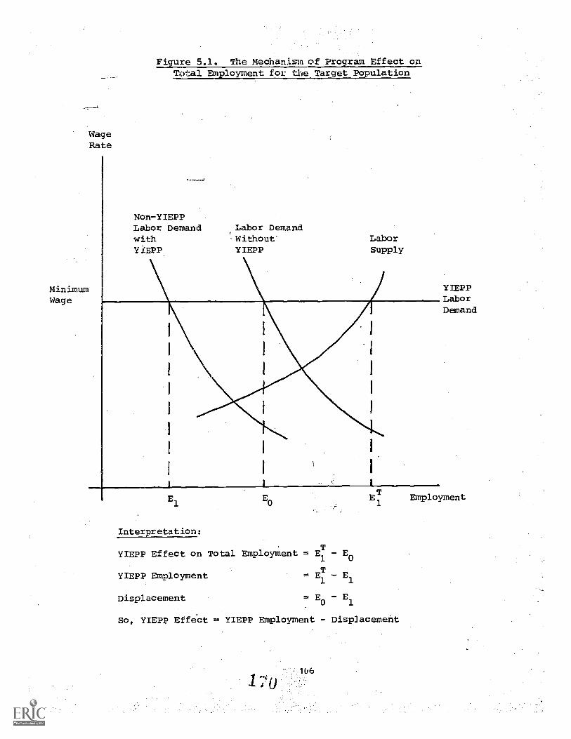
WageRate

Figure 5.1. The Mechanism of Program Effect onTotal Employment for the Target Population

Non-YIEPPLabor Demand Labor Demandwith 'Without' LaborYIEPP YIEPP Supply

Minimum YIEPP

Wage LaborDemand

El E01

E EmploymentT

Interpretation:

YIEPP Effect on Total Employment = ET - Eo1

YIEPP Employment = El - El

Displacement E0

E1

So, YIEPP Effect = YIEPP Employment - Disp3acement

To repeat, the total increase in site-wide employment due to YIEPP

is (ET E0). If there is no displacement, this is also total YIEPP

employment. If there is displacement, with non-YIEPP labor demand shifting

back to E1, displacement is (E0- E

1) and total YIEPP employment is

(ET1

- E1. When a program such as YIEPP is put in place, total employment

shifts out to ET

1.'

youth labor supply at the minimum wage, regardless of

whether displacement is present. However, 'le extent of displacement

determines the number of program jobs that must be funded in order to

achieve this effect. In this chapter we estimate both quantities: the

total YIEPP effect on the employment/population ratio (the percent of

target population hours spent in employment) and net job creation rates

(the ratio of the total YIEPP effect on the employment/population ratio to

total YIEPP employment/population ratio, that is, (ET - E0 ) /(EE

The latter measures the effi-the

E1)). The former LS the program effect.

ciency with which this effect was created.

Definitions of Measures Used to Estimate Program Effects. For each

of the seasonal periods between the summers of 1978 and 1980, we define a

youth's employment/population ratio as the percent of days employed rela-

tive to the total number of days available for employment. The principal

outcome variable in this chapter is the site-wide mean of this employment/

population ratio, calculated separately for those target population youths

who were eligible for YIEPP during each of the periods in question.

Later in this chapter we also estimate program effects on labor

force participation, employment, and unemployment rates. Following stan,

dard conventions, a youth is in the labor force if he or she is either

employed or looking for work. We define the period-specific labor force

participation rate as the percent of days a youth spends in either activ-

ity. Employment and unemployment rates are then, respectively, the percent

of a youth's labor force days spent employed, and the percent of those days

spent unemployed. These measuresfor YIEPP are then compared with those

reported by the Bureau of Labor Statistics, U.S. Department of Labor.

As in the previous chapter, program effects are estimated by

comparing pilot site ratios or rates with those to be expected in the

absence of the program. Where appropriate, we also test for and discuss

107

the possible alteration in these estimates due to sample attrition.

Program effect estimates are reported in the principal tables of this

chapter. Supporting tables are provided in Appendix A, Tables A5.1-A5.11,

means and regression coefficients for the program effect estimates are

reported in Appendix B5, and the attrition calculations are reported in

Appendix C.

Program Effects on the Employment/Population Ratio

Table 5.2 displays employment/population ratios for each of the

preprogram and during-program periods, separately for pilot and control

sites. That is, for those sample youths who were eligible for YIEPP during

the period in question (youths aged 16 to 19 who had not as yet graduated

from high school), we compute the percent of days employed during this

period. These pilot and control site employment/population ratios were

relatively close to each other in the preprogram period, but the pilot site

ratios significantly exceeded those in the control sites during the pro-

gram, indicating a positive YIEPP employment effect. In addition, summer

employment/ population ratios were generally higher than those during the

school year, suggesting that the ratios from these two periods be treated

in two distinct groups.

Program Effects, Separately by Period. Chapter 3 revealed rela-

tively high YIEPP participation rates. As discussed already, if displace-

ment is low, these translate into large employment effects--as shown in

Table 5.3.

This table shows program effects of 21.1, 23.0, 15.5, and 15.7

,percentage points during the school-year periods, for an overall school-

year average of 18.9 percentage points. That is, during the two school

years of program operations, YIEPP is estimated to have raised employment

on average from 21.5 to 40.4 percent, an increase of 87.9 percent over the

level in the absence of the program. These effects .are statistically

significant at better than the 1 percent level.

Program effects during the summers of 1978, 1979, and 1980 are also

large, positive, and statistically significant. at better than a 1 percent

level, but are smaller than those observed for the school year. Across

three summers, the YIEPP employment effect averages 11.8 percentage points,

108

172

Table 5.2. Average Employment/Population Ratios, byPilot orControl Site, and Period

Total Sample SizePilot Control Pilot Control

Preprogram

Spring 1977 7.0 7.6 2,778 1,255

Summer 1977 22.7 26.2 2,778 1,255_

Fall 1977 10.6 12.7 2,778 1,255

During-program

Summer 1978 40.6 26.4 2,353 1,075

Fall 1978 38.2 17.7 2,652 1/188

Spring 1979 42.2 19.8 2,605 1,154

Summer 1979 45.2 34.5 2,362 1,015

Fall 1979 39.1 24.0 2,107 930

Spring 1980 41.3 26.2 2,000 890

Summer 1980 42.3 32.8 1,685 718

Summarya

Preprogram

School-year average 8.4 9.8

Summer average 22.7 26.2 wI

Total preprogramaverage 12.1 13.9 =1 MIR

During-program

School-year average 40.4 22.0 _ - -

Summer average 42.7 31.2 - - -

Total during-programaverage 41.2 25.1 - - _

Note: The sample includes youths who have completed all threewaves of the local field survey and are eligible for the

program during the period in question. See Chapter 2 for

further details. The employment/population ratio is thenumber of weeks employed during a particular period,divided by the total number of weeks in that period.This provides an estimate of the "steady state" employ-ment/population ratio for the period. Unadjusted pilotand control site averages are reported in this table.

aThese are averages of the period-specific ratios reported above,

weighted by the length of each period.

109 173

Table 5.3. Program Effects on Employment/Population Ratios

Estimated pilotsite ratio in

Sample Pilot site the absenceaof P

size ratio the program

School year

Pall 1978 3,840 38.2 17.1Spring 1979 3,759 42.2 19.2Pall 1979 3,037 39.1 23.6Spring 1980 2,890 41.3 25.6

School-year averagec 40.4 21.5

Summer

Summer 1978 3,428 40.6 26.0Summer 1979 3,377 45.2 34.4Summer 1980 2,403 42.3 32.2

Summer averagec 42.7 30.9

'otal during-program averagec

41.2 24.6

This is a regression-adjusted, comparison site mean, fit at pilot site ateristics and preprogram employment. Means of the right-hand-side variacoefficient estimates are reported in Appendix B.

This is the difference between columns 2 and 3, with statistical signifit-statistic on the pilot site dummy variable regression coefficient.

:These are averages of the period-specific ratios reported above, weighteeach period-


raising the employment/population ratio from 30,9 percent in the absence

of YIEPP to 42.7 percent--a 38.2 percent increase. Since YIEPP program

participation is relatively constant between the school year and summer,

the lower summer employment effect is likely to be due to increased dis-

placement during this season. This and related issues are discussed

further in the next section.

With school-year and summer periods combined, we find an overall

YIEPP employment effect of 16.6 percentage points, increasing employment

from 24.6 percent to 41.2 percent. This 67.5 percent increase over the

employment/population ratio expected in the absence of the program is a

very strong result and indicates that YIEPP met its goal of significantly

reducing youth unemployment. (Explicit estimates of program effect on

labor force participation, unemployment, and employment rates are presented

later in the chapter.)

At this point it is useful to assess the effects of sample attri-

tion on our estimates, using the attrition sample data. As noted in

Chapter 2, these data were collected by restricting attention to Hispanics

in Denver/Phoenix and blacks in Baltimore/Cleveland, and undertaking

special efforts to locate youths who dropped from Wave II of the survey.

The resulting attrition sample was subsequently administered both Wave II

and Wave III interviews. Program effect estimates for these and matching

youths who completed all three survey waves are reported in Appendix C,

Table C2.4.

In almost every case, program effects are estimated to be smaller

for the attrition than for the local field survey sample, a result consis-

tent with the observation that attrition sample members exhibited lower

program participation rates than youths who completed all three local field

survey interviews. In the case of Denver, this reduces already low program

effect estimates even closer to zero. (See Table 5.5 and the associated

discussion.) However, the result is not tel.,:ibly striking in view of the

previously noted strong labor market and poor program implementation in

Denver.

The Baltimore/Cleveland attrition sample also shows a reduced YIEPP

employment effect. When this is averaged together with the local field

survey effect estimates for this site, using the attrition rate of 24.4

percent, the result is to reduce program effects estimates by two to four

percentage points. Since this does not significantly alter the overall

finding of strong program effects--in the 10 to 20 percentage point range- -

we feel confident in discounting sample attrition as a significant source

of error in these employment results.

Program Effects for the 15- to 16-year-old Cohort: ;Evidence for

an Ongoing National Program. Recall that'our study sample was constructed

in the spring of 1978, by choosing youths aged 15 to 19 at that time who

had not yet graduated from high school. Thus far, we have focused.on

those youths who continued to meet these eligibility criteria, separately

for each of the during-program periods, from the summer of 1978 to the

summer of 1980. However, this procedure averages together the effects

experienced by youths who aged through the program (those who were 15 to 16

years of age at program start-up) and the effects experienced by youths who

were beyond age 16 at program start-up. Since effects may differ across

these two groups, and since, if they do, the responses of the former group

alone are most relevant to an ongoing national program, Table 5.4 shows

the employment effects for the 15- to 16-year-old cohort.

Comparison of Tables 5.3 and 5.4 shows that restriction to the

15- to 16-year-old cohort raises YIEPP employment effects from 18.9 to 21.2

percentage points during the school year, and from 11.8 to 13.5 percentage

points during the summer. Over the full program period, the average

employment effect increases from 16.6 to 18.6 percentage points, a rise of

12 percent.

As a final step, we have computed effects for the 15- to 16-year-

old cohort, with Denver and Phoenix deleted from the sample. This yields a

measure of program effect for an ongoing national program, fully imple-

mented in distressed labor markets. As reported in Appendix A, Table A5.4,

these effects are larger still, averaging 24.6 percentage points during the

school year and 14.4 percentage points during the summer, for an overall

average of 21.3 percentage points during the program period. This is an

increment of 109.2 percent over the employment/population ratio expected in

the absence of YIEPP.

Table 5.4. Program Effects on Employment/Population Ratiosfor the 15- to 16-Year-old Cohort, Separately by Period

Estimated pilot Program effect assite ratio in a percent of ratio

Sample. Pilot site the absence of Program in the absence. of _

size ratio the program effect the program

School year

Fall 1978Spring 1979Fall 1979Spring 1980

School-year averagec

Summer

Sumier'1978Summer 1979Summer 1980

Summer averagec

Total during-program averagec

2,005 34.7 11.3 23.4*** 207.1

2,053 39.4 15.9 23.5*** 147.8

1,920 40.5 21.5 19.0*** 88.4.

1,914 43.0 24.2 18.8*** 77.7

39.6 18.4 21.2*** 115.2

1,515 39.5 22.5 17.0**t 75.6

1,980 45.4 34.3 11.1*** 32.4.

1,685 43.6 31.1 12.5*** 40.2

42.8 29.3 13.5*** 46.1

40.7 22.1 18.6*** 84.2

aThis is a regression-adjusted, comparison site mean, fit at pilot site average personal charac-teristics and preprogram 'employment. Means of the right-hand-side variable and regression;coefficient estimates=are reported in Appendix B.

bThis is the difference between columns 2 and 3, with statistical significance computed from thet-statistic on the pilot site dummy variable regression coefficient.

cThese are averages of the period-specific rates reported above, weighted by the length ofeach period.


A

Pro ram Effects, Separately by site. AS previously noted, the

pilot/comparison site pairs differ significantly in labor, market conditions

and program implementation, so that it is useful td, di0;7gregate the

program effect estimates by site. These results are displayed in Vab4e

5.5, which shows school-year, summer, and total grog Am effects, caliated

from regression-adjusted, period=-specific mean diffetchoR:g for eael:bf the

during-program periods, from the summer of 1978 to the eumawr of 1980.

These are then averaged, following the procedure emptoyed in Table 5.3.

(The sample sizes underlying these calculations are repOrted in Appendix A,

Table A5.I. The regression calculations are reported in Appendix B.)

Ths most obvious finding in this table is that the Denver YIZFP

employment effects are very much smaller than those -ifthe other sites.

This is probably due to two factors. First, as noted in previltIns chapters,

total labor demand was considerably stronger in Denver/PhNenix than in tie

other sites. 1 Where demand is close to meeting suL2p11M at the federal

minimum wage, the prograM effect will be small. (Pec611 Figure 5.1.)

Second, as also noted in previous chapters, program ImpIeserftation in

Denver was relatively poor, leading to a freeze on intake ;,)f new partici-

parits in June, 1979. To the extent that the prciTram was never properly

implemented' in Denver, results from this site do not accurately estimate

program effects. Of course, it may be that pootr implementation was at

least partly due to a lower level of enthusi4sm for the program, in turn,

perhaps because of the strong local labor market that made the program

appear to be less necessary. In any case, the results suggest that future

YIEPP -like programs should be concentrated in areas with relatively dis-

tressed local labor markets.

The three remaining sites in Table 5.5 show very s'rong and similar

effects. In each case the school-year effect is significantly larger than

the summer effect, and all are statistically significant at better than

1 Evidence on the relative strength of labor demand in Denver/Phoenixincludes the unemployment rates of Table 5.1, estimated target populationpilot site employment/population ratios in the absence of the program(column 2 of Table 5.5), and the relatively high target population wage

ratesin Denver/Phoenix during the pre-program summer (Barclay et al.(1979); Farkas, Olsen and Stromsdorfer (1981).

114

178

Table 5.5. Program Effects on Employment/Population Ratios, Separately by Site


site ratio in a percent of ratio

Pilot site the absence of Prograg in the absence of

ratio the program effect the program

Denver

School-year aysragec 39.6 37.3 2.3 6.2

Summer average 45.3 38.6 6.7* 17.4

Total during-program averagec. 41.5 37.7 3.8 10.1

Cincinnati

School-year average. 35.5 18.6 16.9*** 90.9

Summer average 36.4 26.1 10.3*** 39.5

Total during-program average 35.8 21.1 14.7*** 69.7

Baltimore

School-year average 47.2 22.6 24.6*** 108.8

Summer average 47.6 36.3 11.3*** 31.1


Mississippi


Summer average 38.5 27.2 11.3*** 41.5


a.This is a regression-adjusted, comparison site mean, fit at pilot site average personal charac-

teristics and preprogram employment. Means of the right-hand-side variables and regression

coefficient estimates are reported-in Appendix B.

bThis is the difference between columns 1 and 2, with statistical significance Computed from the

t-statistic on the pilot site dummy variable regression coefficient.

cThese are averages of the period-specific ratios weighted by the length of each period.'

* = significant at the 10 percent level.*** = significant at the 1 percent level.

179

a 1 percent level. The three summer effects 7:-!-e at the 10 to 11 percentage

point level; the school-year effect is 16.9 percentage points in Cincin-

nati, 24.6 percentage points in Baltimore, and 17.8 percentage points

in Mississippi. These results are consistent with our previous finding of

a stronger school-year than summer employment effect (Farkas et al. 1980).

This finding may be due to the narrowed gap between summer minimum wage

supply and demand in the absence of YIEPP, resulting from subsidized

employment provided by the federal Sumn$:" Youth Employment Program (SYEP)

during the summer periods in question. Thus, it is possible that if YIEPP

were to be implemented in the years ahead, with the reduced funding for

°the.: subsidized employment programs that current legislative proposals

suggest, summer YIEPP employment effects would more closely approximate the

school-year effects of Table 5.5.

In sum, with the exception of Denver, YIEPP employment effects are

uniformly large and significant. As a result of the program, summer

employment for target population youths increased IT 31 to 42 percent,

while school-year employment for these youths increased by 91 to 109

percent.

Program Effects by Economic Sector. A potentially important YIEPP

innovation was the placement of some youths in subsidized private sector

jobs. The extent of stmh placement varied by site and over time, with

greater use of private sector positions occurring toward the end of the

demonstration. However, since the long run goal of the demonstration was

to increase postprogram employment and earnings, and since during-program

private sector employment may be more efficacious than similar public

sector employment, the during-program sectoral employment impacts of

YIEPP are of some interest.

These impacts are reported in Table 5.6. 1 It is immediately

clear that private sector employment effects are significantly smaller than

1Youths are coded as employed in the private sector if they describedthemselves as "an employee of a company or business for wages, salary, orcommission," or as "an employee of an individual or family for wages orsalary." Youths are coded as employed in the public sector iftheydescribed themselves as "a federal, state, or local government employee,"or as "an employee of a church or charitable organization."

116

Table 5.6. Program Effects on Employment/Population Ratios, Separately by Sector

Estimated pilot Program effect assite ratio in a percent of retic

Sample Pilot site the absence of PrograT in the absence of

size ratio the program effect the program

A. Private Sector Employment

School year

Fall 1978 3,840 16.3 12.6 3.7*** 29.4

Spring 1979 3,759 18.5 14.0 4.5*** 32.1

Fall 1979 3,037 21.5 18.3 3.2** 17.5

Spring 1980 2,890 22.8 19.2 3.6*** 18.8

School-year averagec 19.9 16.1 3.g * ** 23.6

Summer

Summer 1978 3,428 16.3 15.4 0.9 5.8

Summer 1979 3,377 21.3 21.4 - 0.1 0.5

Summer 1980 2,403 26.1 21.8 4.3*** 19.7

Summer average 21.2 19.5 1.7 8.7

Total during-program averagec --- 20.3 17.2 3.1*** 18.0

B. Public Sector Employment

School year

Fall 1978 3,840 22.0 4.5 17.5*** 388.9

Spring 1979 3,759 23.7 5.4 18.3*** 338.9

Fall 1979 3,037 17.6 5.3 12.3*** 232.1

Spring 1980 2,890 18.5 6.4 12.1*** 189.1


181

Table 5.6. (Continued)

Estimated pilot Program effect asite 'ratio in a percent of rat

S4mple Pilot site the absenceaof ErograE in the absence oW.ze ratio the program effect the program

Summer

Summer 1978 3,428 24.3 10.9 13.4*** 122.9Summer 1979 3,377 23.9 13.2 10.7*** 81.1Summer 1980 2,403 16.2 10.3 5.9*** 57.3

Summer average 21.5 11.5 10.0*** 87.0

Total during-program average --- 20.8 7.5 13.3*** 177.3

aThis is a regression-adjusted, comparison site mean, fit at pilot site average personal charac-teristics and preprogram employment. Means of the right-hand-side variables and regressioncoefficient estimates are reported in Appendix B.

bThis is the difference between columns 2 and 3, with statistical significance computed from thet-statistic on the pilot site dummy variable regression coefficit.

cThese are averages of the period-specific ratios reported above, weighted by the length ofeach period.

** = significant at it-, a percent level.*** = significant at the 1 percent level.

1S2

those in the public sector. During the school year, private sector effects

range between 3.2 and 4.5 perCentage points, with an overall average of

3.8 percentage points. This effect is statistically significant, and

increases private employment by 23.6 percent over the level expected in the

absence of the program--a respectable, but not overwhelming effect, espe-

cially in comparison to the public sector effect of about 273 percent.

The private sector effect is smaller still during the summer,

averaging 1.7 percentage points, an increase of 8.7 percent aver the level

expected in the absence of the program. However, this effect is not

statistically significant. With school year and summer combined, the total

private sector employment effect is a statistically significant 3.1 percen-

tage points, an increase of 18 percent over the level of 17.2 percentage

points expected in the absence of YIEPP.

Public sector employment effects are very much larger, averaging 15

percentage points during the school year, and 10 percentage points daring

the summer -- increases respectively of about 273 and 87 perrNatt

levels expected in the absence of YIEPP. With school yerixrairiunmer

combined, the public sector employment effect is 13.1 percepiE5--an

increase of about 177 percent over the 6Tpected in ther;.:41:ca of the

program.

The disparity between the malY- of the public and private

sector employment effects has two ;,..Auses. First, YIEPP job hours

were predominantly in the public rather than the private sector. Second,

pri ".t *ector displacement appears to be higher than public sector

displacement. These findings are examined in the next section.

Program Effects, Separately by Race and Sex. YIEPP enrolled black

youths most heavily. The consequences of this program employment

effects are shown in Table 5.7.

All effects are positive, but not all are statistically significant

and they vary widely across race/sex groups The largest effects are for

black females--24.7 percentage points during the school year, and 15.7

percentage points during the summer. Overall, the black female employment

effect is '21.7 percentage points--an 4.ncrease of 128 percent over the level

expected in the absence of the program.

119

Table 5.7. Program Effects on Employment/Population Ratios Separately byPeriod, Sex, and Race :7

Estimated pilotsite ratio in

Pilot site the absence ofratio the program

Program effect asa percent of ratio

PrograE in the ahsence ofeffect the program

White male

School-year averagec

46.6 34.5 12.1** 35.1

Summer averagesc

Total during-program average47.046.7

42.637.2

4.49.5*

10.3

25.5

Black male

School _,ear average 43.0 21.2 21.8*** 102.8

Summer average 46.5 34.4 12.1*** 35.2

Total during-program average 44.1 a5.6 18.5*** 72.3

Hispanic male

School-year average 51.3 47.9 3.4

Summer average 55.1 50.0 5.1 10.2

Total during-program average 52.6 58.6 4.0 8.2

White female

School-year average 29.1 25.3 3.8 15.0



Black female

School-year average 18,5 13.8 24.7*** 179.0

Summer average 39.0 23.3 15.7*** 67.4Total during-program average.; 38.7 17.0 21.7*** 127,6

1j1

Fable 5.7. (Continued)


site ratio in a percent of ratio

Pilot site the absence of Prograg in the absence of

ratio the programa

effect the program

Hispanic female


Summer average 41.8 27.3 14.5** 53.1

Total during-program average 36.2 29.3 6.9* 23.5

White

School41,year average. 37.0 29.4 7.6** 25.9



Black


Summer average 42.6 28.7 13.9*** 48.4

Total during-"program average 41.3 21.1 20.2*** 95.7

Hispanic


Sumner average 48.0 38.1 9.9* 26.0

Total during- program average 43.8 38.2 5.6 14.7

1 35


Estimated pilot Program effect assite ratio in a percent of ratio

Pilot site the absence of Prograg in the absence ofratio the program effect the program

Male

School-year average 44.2 26.7 17.5*** 65.5Summer average 47.4 37.6 9.8*** 26.1


Female

School-year average 36.9 17.3 19,6*** 113.3

Summer average 38.4 24.7 13.7*** '55.5


aThis is a regression-adjusted, comparison site mean, fit at pilot site average personal charac-teristics and preprogram employment: Means of the right-hand-side variables and re4ressioncoefficient estimates are reported in Appendix B.

bThis is the difference between columns 1 and 2, with statistical significance computed from thet-statistic on the pilot site dummy variable regression coefficient.

cThese are averages of the period-specific ratios weighted by the length of each period.

* = significant at the 10 percent leVel.** = significant at the 5 percent level.


1.SG

Next in magnitude are the effects for black males, 21.8 percentage

points during the school year and 12.1 percentage points during the summer,

for an overall average of 18.5 percentage points, an increase of 72.3

percent over the rate expected in the absence of the program. It appears

that both black males and females were strongly attracted to the program,

with black females experiencing the larger employment effect because of the

larger gap between minimum. wage supply and demand in the absence of the

program for this group. This result also suggests, but does not confirm,

the possibility of racial discrimination in the absence of the YIEPP

program. (See columns 1 and 2 of Table 5.7, and recall Figure 5.1.)

The other statistically significant effects are for white males

during the sclool year and for Hispanic females during the summer. White

males are present in our study sample in all eight sites, and we therefore

have no reason to doubt these findings. Some white males did join YIEPP,

probably because employment in the absence of the program was more diffi-

cult to find duxing the school year than during the summer. The absence of

a statistically significant effect for white females is also understand-

able--these youths were the least likely to join the program.

The effects for Hispanics are less trustworthy, since almost all

Hispanics were in Denver/Phoenix, and Denver's project was imperfectly

implemented. However, the significant effect for Hispanic females can be

understood in light of two general observations. First, Hispanics of both

sexes were reasonably attracted to ';71EPP. Second, female Hispanics, like

females of all races in our sample, experienced particular difficulty

finding employment 'in the absence of the program.

Net Job Creation

As discussed at the beginning of the chapter and portzayed in

Figure 5.1, the difference between YIEPP program employment and its effect

in increasing site -wide employment is the extent of displacement, that is.

YIEPP funding of jobs that would have been available even in the absence of

the program. The complement of the displacement rate is the net job

creation rate, which is defined as the ratio of the YIEPP employment

effect to YIEPP program employment. The net job creation rate measures the

efficiency with which the YIEPP employment effect was achieved. If this

123 1 8 1'

rate were equal to its maximum attainable value, 1.0, every YIEPP job hour

would have led to a full one-hour increment for site-wide employment over

the regular employment level in the absence of the program. If this rate

were equal to its minimum, 0.0, there would have been no net job creat!

YIEPP would have simply subsidized jobs available in any event. Between

these two extremes, the net job creation rate measures the percent of each

YIEPP employment hour that provided employment that would not have been

otherwise available. This is a straightforward measure of program job

creation efficiency.

Table 5.8 reports these net job creation rates for total and

sectoral employment. For total emploYment, the school-year net job crea-

tion rate was 66.8 percent, and the summer net job creation rate was 43.5

percent, leading to an overall during-program average of 59.5 percent.

Although the programs are not strictly comparable, it is instructive to

note that the resulting displacement rate of 40.5 percent is higher than

that of previous field-monitoring estimates of CETA Public Service Employ-

ment (PSE) (Nathan et al. (1981)). It is also lower than previous aggre-

gate data econometric estimates of CETA (PSE) displacement (Johnson and

Tomola (1977)). Of course, our estimates only measure YIEPP displacement

for the target population, and so provide a lower bound on total YIEPP

displacement. In addition, our estimates cover a different time period

and, as noted, a different program. In particular, YIEPP, unlike CETA PSE

during the 1970s, involved significant private sector job plae..../ As

shown in Table 5.8, such private sector subsidized employment is apparently

accompanied by higher displacement than is subsidized public sector employ-

ment.

The second panel of this table shows school-year private sector

employment with a net job creation rate of 52.8 percent, 14 points below

the overall school-year average. During the summer, net private sector job

creation fell to 26.6 percent, leading to an overall private sector

average of 44.9 percent. By contrast, net public sector job creation

was 80.2 percent during 'the school year and 54.6 percent during the summer,

for a public sector average of 71.5 percent.

Put in different terms, only 1.40 jobs had to be created or iden-,,

titled in the public sector in order to employ one YIEPP participant, while

124

Table 5.8. Net Job Creation, by Season and Period

Program Effect Programon Employment/ Employment/ Net Job

Population Population Creation

Ratio Ratio Rate

A. Total Employment

School year

Fall 1978 21.1 28.9 73.0

Spring 1979 23.0 31.7 72.6

Fall 1979 15.5 26.1 59.4

Spring 1980 15.7 26.1 60.2

School-year averaged

18.9 28.3 66.8

Summer

Summer 19 78 14.6 28.4 51.4

Summer 1979 10.8 31.8 34.0

Summer 1980 10.1 21.1 47.9

Summer averaged 11.8 27.1 43.5

Total duriaq-program16.6 27.9 59.5average

B. Private Sector Employment

School year

Fall 1978 3.7 6.0 61.7

Spring 1979 4.5 7.6 59.2

Fall 1979 3.2 7.5 42.7

Spring 1980 3.6 7.5 48.0

School-year averaged 3.8 7.2 52.8

Sumner

Summer 19 78 0.9 4.6 19.6

Summer 1979 - 0.1 7.7 - 1.3

Summer 1980 43 7.0 61.4

Summer averaged 1.7 6.4 26.6

Total during- program3.1 6.9 44.9average

125 1SJ


Program Effecton Employment/PopulationRatio

ProgramEmployment/ Net JobPopulation CreationRatio Rate

C. Public Sector Employment

School year

Fall 1978 17.5 20.1 87.1

Spring 1979 18.3 21.8 83.9

Fall 1979 12.3 16.2 75.9

Spring 1980 12.1 16.4 73.8

School-year averaged

15.0 18.7 80.2---

Summer

Summer 1978 13.4 20.5 65.4

Summer 19iJ 10.7 21.8 49.1

Summer 1980 5.9 12.8 46.1

Summer Averaged

10.0 18.3 54.6

Total during-program13.3 18.6 71.5average

aReported in Tables and 5.6.

bThis is the employment/population ratio in program jobs; theaverage number of weeks spent by eligible youths in program.jobs during each period divided by the number of weeks in thatperiod. These ratios have been calculated from the data alsoused for the analyses repoezed in Chapter 3.

cColumn 1 divided by column 2.

dThese are averages of the period-specific ratios reportedabove, weighted by the length of each period.

2.23 such jobs had to be created in the private sector to employ one YIEPP

participant.1

The message for policy seems clear. Private sector placements may

lead to better postprogram -Outcomes than public sector placements, but.

private sector placements are achieved at .a higher cost to the program

budget because of displacement. There is a tradeoff between higher quality

jobs (closer to "real" jobs rather than "make-work") and net job creation.

Wolfhagen (1981); Diaz and Ball (198 and Welch et(See also Ball and al.

forthcoming.)

Program Effects on Labor Force Participation, Employment, and Unemploy-

ment Rates

Table 5.9 displays labor force participation, employment, and

unemployment rates for pilot and control sites in the pre-program and

during - program periods. The labor force participation rate is the percent

of days employed or looking for work, and the employment and unemployment

rates are, respectively, the share of these days spent at each activity:

The general impression is one of increasing labor force participation and

employment and decreasing unemployment for our sample over time, accom-

panied by a positive program effect on the former two rates, and a negative

program effect on the latter rate. These effects are shown in Table

5.10.

Program Effects, Separately by Period. Table 5.10 shows a positive

YIEPP labor force participation effect of 17.5 percentage points during the

school year and 12.1 percentage points during the summer, for an overall

effect of 15.7 percentage points, an effect statistically significant at

better than the 1 percent level. This represents an increment of 44

percent over the labor force participation rate expected in the absence of

the program.

As the table also shows, employment rate effects are large and

positive, averaging 19.7 percentage points during the school year and 11.7

percentage points during the summer, for an overall average of 16.9 percen-

tage points, an increment of 53 percent over the level expected in the

absence of YIEPP.

The 2.23 figure, for example, is calculated as follows: 100.0/44.9 =

2.23.

127 191

.Table 5.9. A'.rerage Labor Force Participation, Employment,and Unemployment Rates, by Pilot or Control Site and Period

Labor forceparticipation rate

EmploymEntrate

UnemployTentrate-

SampleSize

Pilot Control Pilot Control Pilot Control Pilot Contro:

Preprogram

Spring 1977 9.5 11.3 9.8 12.4 90.2 87.6 2,778 1,255

Summer 1977 35.7 39.8 29.7 35.4 70.3 64.6 2,778 1,255

Fall 1977 14.0' 16.0 18.6 20.6 81.4 79.4 2,778 1,255

During-programd

Summer 1978 ,49.2 1 34.9 50.1 35.5 49.9 64.5 2,353 1,075

Fall 1978 46.7 i 27.2 45.2 24.1 54.8 75.9 2,652 -1,188

Spring 1979 50.9L 29.8 50.0 27.3 50.0 72.7 2,605 1,154

Summer 1979 54.6 , .i.ip43.3 53.7 45.0 46.3 55.0 2,362 1,015

Fall 1979 50.7' 38.0 44.4 28.5 55.6 71.5 2,107 930

Spring 1980 52.8 38.8 48.5 32.9 51.5 67.1 2,000 890

Summer 1980 55.2 45.9 50.4 40.2 49.6 59.8 1,685 718

Summary

Preprogram

School-yearaverage 11.5 13.4 20.7 25.0 79.3 75.0 - - -

Summer average 35.7 39.8 29.7 35.4 70.3 64.6 ma gm= ma - - -Total preprogram

average 17.6 20.1_ 32.9 39.3 67.1 60.7

During-program

School-yearaverage 50.5 33.6 47.3 28.4 52.7 71.6 - - - - - -

Summer average 52.9 41.3 51.3 40.2 48.6 59.7

Total during-programaverage 51.3 36.2 48.6 32.3 51.4 67.6 - - -

aThe labor force participation rate is the number of weeks either employed or lookingfor work during a particular period, divided by the total number of weeks in thatperiod. Unadjusted pilot and control site averages are reported in this table.

bThe employment rate is the number of weeks employed during a particular period,divided by the number of weeks in the labor force (employed or looking for work)during that period.

cThe unemployment rate is the number of weeks looking for work during a particularperiod, divided by the number of weeks in the labor force during that period.

Preprogram unemployment (and, consequently, labor force participation) rates weremeasured differently from during-program rates. In the latter period each youth'wasquestioned about job search for each of his nonemployment periods. In the earlierperiod, not employed youths who were enrolled in school were assumed to be. notlooking for work., As a result, when other things are equal, our during-programunemployment will be measured as higher than preprogram unemployment. However,

since this will be true in both pilot and control sites in the preprogram period,it introduces no bias into program effect estimates.eThese are averages of the period-specific rates reported above, weighted by thelength of each period.

128

192

Table 5.10. Program Effects on Labor Force Participation,Employment, and Unemployment Rates

Estimated pilot Programeffectsite rate in the a percent of ri

Sample Pilot site absence of the Prograt in the absencea

size rate program effect the program

A. Labor force participation rate

School` year

Fall 1978 3,840 46.7 26.5 20.2*** 76.2

Spring 1979 3,759 50.9 29.1 21.8*** 74.9

Fall 1979 3,037 50.7 37.7 13.0*** 34.5

Spring 1980 2,890 52.8 38.2 14.6*** 38.2

School-year averaged - - - 50.5 33.0 17.5*** 53.0

Summer

Summer 1978 3,428 49.2 34.4 14.8*** 43.0

Summer 1979 3,377 54.6 43.0 11.6*** 27.0

Summer 1980 2,403 55.2 45.2 10.0*** 22.1

Summer averaged

ammo ow 53.0 40.9 12.1*** 29.6

Total during-program averaged 51.3 35.6 15.7*** 44.1

B. Employment ratec

School year

Fall 1978 3,840 45.2 23.4 21.8*** 93.2

Spring.1979 3,759 50.0 26.2 23.8*** 90.8

Fall 1979 3,037 44.4 27.9 16.5*** 59.1

Spring 1980 2,890 48.5 32.2 16.3*** 50.6

School-year averaged - - 47.3 27.6 19.7*** 71.4


7,stiMated. pilot Program effect assite rwte in the a percent of ratio:`.

Samplesize

Pilot siterate

.absenceaof the

program -PrograEeffect

Summer

Summer 1978 3,428 50.1 34.7 15.4***

Summer 1979 313'77 53.7 . 44.9- 8.8***

Summer 1980 2,403 50.4 39.6 10.8***

Summer averaged

51.4 39.7 11.7***

Total during-program averaged

48.6 31.7 16.9***

C. Unemployment rates

School year

Fall 1978 3,840 54.8 76.6 -21.8***Spring 1979 3,759 50.0 73.8 23.8***

Fall 1979 3,037 55.6 72.1 -16.5***

Spring 1980 2,890 51.5 67.8 -16.3***.

School-year averaged . 52.7 72.4 -19.7***

Summer

Summer 1978 3,428 49.9 65.3 -15.4***.

Summer 1979 3,377 46.3 .55.1 - 8.8***

Summer_1980 2,403 49.6 60.4 -19.8***

Summer averaged

48.6 60.3 -11.7***

Total during-program avera ed

51.4 68.3 -16.9***

in tbi.'absenceofthe program

19.6

27.3

29.5

53.3

-285-32.2-22.9-24.0

-27.2

-23.6- 16.0

-17.9

-19.4

- 24.7

a,bSee notes to Table 5.2.

See notes 1-4 of Table 5.9. 194dthese are averages of the period-specific rates reported above, weighted by the length f eachperiod.

Unemployment.1 Since the employment and unemployment rates must

always sum to-1.0, any program effect on one of these quantities is neces-)'

sarily accompanied by an equal and opposite program,_ effect on the other:

Accordingly, we find that YIEPP decreased school-year unemployment by 19.7

percentage points, and decreased summer unemployment by 11.7 percentage

points, for an overall unemployment rate decrease of 16.9 percentage

points. This lowered target population unemployment by-24.7 percent below

the level expected in the absence of the program.

Program Effects for the 15- to 16-year-old Cohort

Table 5.11 shows that restricting the sample to the 15- to 164ear-

old cohort increases labor force participation rate effects from 17.5 to

19.6 percentage points during the school year and from 12.1 to 13.7 percen-

tage points during the summer. Employment rate effects increase from 19.7

to 22.5 percentage points during the school year, and from 11.7 to 12.5

.percentage points during the summer. (Of course, unemployment rate effects

change by equal and opposite amounts.)

When Denver and Phoenix are excluded, school-year.labor force

participation rate effects increase to 22.7 percentage points, and summer

labor force participation rate effects increase to 17.7 percentage paints,

while school-year employment rate effects increase. to 26.2 percentage

points, and summer employment rate effects remain at 12.5 percentage

1Dints. (See Appendix A, Table A5.9.) Once again, we find a small but

noticeable increase in the effect for the younger cohorts, which suggests

that the program effect for an ongoing national program will have a large

and significant effect on the target population of disadvantaged youth.

1--Note again that the unemployment rate is the total weeks looking for work

during a period divided by the total weeks in the labor force for that

period. The measured unemployment rate is somewhat higher than thatofficially-calculated by the Bureau of Labor Statistics, 'U.S. Department

of Labor since job search is, in effect, smoothed over the entire period

of labor force participation. The relative levels and absolute differ-

ences in the unemployment rate between pilot and the comparison sitesshould, however, be free of bias.

Table 5.11. Program Effects on Labor Force Participation, Employment, andUnemployment Rates for. the 15- to 16-Year-old Cohort, Separately by Period

Sample Pilot sitesize rate

N\ Labor force Earticipation rate

School year

Fall 1978 2,005 43.0

Spring 1979 2,053 47.8

Fall 1979 1,920 51.0

Spring 1980 1,914 53.4

School-year averagec 49.0

Summer

Summer 1978 1,515 47.5

Summer 1979 1,980 53.9

Summer 1980 1,685 55.7

Summer averagec - - - 52.4

total during-program average 50.1

B. Employment rate

School year

Fall 1978 2,005 42.0

Spring 1979 2,053 47.2

Fall 1979 1,920 46.0

Spring 1980 1,914 51.0

School-year average4 46.8

Estimated pilotsite rate in theabsenceaof theprogram

Program effect asa percent of rate

Program in the absence ofeffect the program

20.3 22.7***

25.0 22.8***

35.0 16.0***36.7 16.7***

29.4 19.6***

30.2 17.3***

41.5 12.4***

44.5 11.2***

38.7 13.7***

32.5 17.6***

111.891.245.7

45.5

66.7

57.329.925.2

35.4

54.2

17.4

22.226.0,

30.6

24.6***25.0***20.0***20.4***

22,5***

141.4112.676.966.7

92.6

able 5.11. Continued)Estimated pilot Program effect as

site rate in the a percent of rate

Sample. Pilot site absence of the PrograB in the absence of


mutter .

mnmer 1978 1,515 48.6 31.8 16.8*** 52.8

wnmer 1979 1,980 54.2 46.6 7.6*** 16.3

wnmer 1980 1,685 52.3 39.2 13.1*** 33.4

dwnmeraverage 51.7 39.2 12.5*** 31.9

Dtal during-program averaged --- 48.5 29.3 19.2*** 65.5

Unemployment rate

chool year

all 1978 2,005 58.0 82.6 -24.6*** -29.8

pring 1979 2,053 52.8 77.8 -25.0*** ' -32.1

all 1979 1,920 54.0 74.0 -20.0*** -27.0

pring 1980 1,914 49.0 69.4 -20.4*** -29.4

chool-year averaged

53.2 75.7 -22.5*** -29.7

urnmer

wmmer 1978 1,515 51.4 68.2 -16.8*** -24.6

mmmer 1979 1,980 45.8 53.4 - 7.6*** -14.2

ummer 1980 1,685 47.7 60.8 -13.1*** -21.5

wnmer average-- 48.3 60.8 -12.5*** -20.6

otal during-program averaged 51.5 70.7 -19.2*** -27.2

See notes to Table 5.3.

dThese are averages of the period-specific rates reported above, weight.ed by the length of

each period.

*** = significant at, the 1 percent level.

197

Program Effects,="Separately by Site. The total program labor force

participation, unemployntent, and employment rate results reported above

generally replicate those for employment/population ratios. These are

strong positive effects, with larger magnitudes during the school year than

during the summer. Similarly, when these effects are examined separately

by site, they generally relaicate the site-specific results for the employ--

ment/population ratio. Thus, as shown in Appendix A, Table A5.5, labor

force participation, employment, and unemployment rate effects are small,

and not statistically significant for Denver. The other three sites show

strong, positive and similar effects, the only departure from the pattern

of previous results reported on the employment/population ratio being

somewhat smaller YIEPP labor force° participation effect in Cincinnati.

Program Effects, Separately by Race and Sex. Effects for race/sex

subgroups also, generally replicate those reported above As shown in

Appendix A, Tables A5.6, A5.7, and A5.8,. very large and positive effects

are found for black females and black males, with strong effects also for

Hispanic females during the summer. Smaller effects are found for white

and Hispanic males, and no significant effects are found for white females.

Employment/Population Ratios and Wage Rates for Employed Youths

Having found-Strong, positive, labor force and employmen effects

of the YIEPP program on the sample as a whole, it is useful to examine

briefly the employment and wage characteristics of.employed youths. 'd1 As

shown in Appendix A, Table A5.10, even in the absence of YIEPP (in :;(theji

preprogram period and in control sites), period-specific employment/nopu-,---

_

lation ratios for youths employed-at'all during a particular period are

quite high--in the 60 to 70 percent range. In the pilot sites during the

program these ratios increase by an additional 5 to 10 percentage points.

This suggests that the principal YIEPP employment effect acts through

increasing the rate of transition from the "not employed" to the "employed"

state, but that there is also" an additional, though smaller, YIEPP effect

in increasing the percent of time employed by working youths.

As for wage rate effects of the program, Table A5.11 in Appendix-

A suggests that'these are minimal or nonexistent. During the program

period, in both pilot and control sites, during the school year and the

summer, median wage rates are close to the minimum wage, with little

.evidence of an effect due, to YIEPP. However, these wages are much more

*tightly clustered around the median for in-school than for out-of-school

youths, 'suggesting that as target population youths age into their post--

program period, greater wage variation will be evidenced. This will be

explored in the Final Report to be completed in 1983.

Comparison with United States Average Employment and Unem loyment Statistics

As is waP kDOwn, employment and labor .force activity rates often

differ significant3y across surveys, particularly for youths. (See Freeman

and Medoff (1982)) In the interests of comparing our survey results with

the current Population Survey results used to report United States averages

by the Bureau of Labor Statistics (BLS), we attempted to approximate. BLS

methodology with our data. That is, for all sample youths aged 16 to 19

(not just the program-eligible subgroup), we counted as employed those

youths who reported working at all during the week that included the 12th

day of oCtober, 1978. From this we computed pilot and control site

employment/population ratios for race/sex groups. Then, among youths not

employed according to this measure, we counted as unemployed all those who

reported looking for work during this or any of the preceding four weeks.

From this we computed pilot and control site unemployment/population

ratios for race/sex groups. (For a description of this methodology as

applied by the Bureau of Labor Statistics, see the Appendix to any issue ofr,

Employment and Earnings.) Our results, along with those of the BLS, are

reported in Table 5.12.

Comparing our control site results with BLS calculations of United

States averages, we find generally the same race/sex pattern but different

overall levels in the two sets of results. That is, both.we and the BLS

find the highest employment/population ratios for white males, followed

in order by white females, black males, and black females. For unemploy-

ment/population ratios the order is reversedvthe highest rates are for

black females, followed by black males, white females, and white males.

(We find higher unemployment for white females than for white males,_

however, whereas the BLS finds the reverse.)

Table 5.12. Employment/Population and Unemployment /PopulationRatios,for,-16- to-19-year-old-Youths by Race, and Sex:'

":,YIEPP Sample and United States'Averages forOctober 1978

Whitefemales

Blackfemales

Whitemales

Blackmales

Employment ratioa

Pilot sites 47.4 41.9 29.2 38.7

Control sites 31.4 18.6 20.9 10.6

United States 54.9 28.1 48.7 22.1

Unemployment ratioa

Pilot sites 29.3 31.6 27.3 29.7

Control sites 18.6 41.4 28.7 45.6

United States 8.5 12.4 7. 4 13.4

Note: To increase comparability with United States averagescalculated from the Current Population Survey, employ-ment/population and unemployment/population ratios'werecalculated for_this table as follows. Attention isrestricted to 'youths 16 to 19 years of aoe during therelevant period, who completed all three'Waves of thelocal field survey;-this includes youths,who were pro-gram ineligible due to high,school.graduation. A youth

-is considered-to be-employed if 'he-worked at.all-duringthe week which included the i2th day of 06tober 1978.-

Of not employed youths, those who looked.for work during

this or any of the preceding four.weeks are considered'tobe unemployed. United States averages were calculated.for the civilian population from statistics.reported in

the November, 1978 issue of Employment and Earnings; For

blacks we use the statistics for "black and other."

aBecause these employment/population and Unemployment/population ratios have been specially calculated usinga methodology designed to maximize comparability withnational (CPS) statistics, they are not directly compa-rable with the other measures in this chapter. However,

they could be used to calculate labor force participa-tion, employment, and unemployment ratesbased on CPSmethodology; -e7g,. labor-force-participatkon-rate =employment/population ratio + unemployment/populationratio; employment rate = (employment/population ratio)/labor force participation rate; unemployment rate =(unemployment/Population ratio)/labor force participa-

tion rate,

Our control site employment/population ratios are from 10

percentage points lower than those reported by the BLS, whereas our,control

site unemployment/population ratios are from 10 to 30 percentage' points

higher. Since our study sample was drawn from disadvantaged youths in

weaker than average labor markets,: these differences in level are in the

direction expected. No doubt, however, they also contain at least some

residual differences associated with different survey and measurement

methodologies.

Summary

The results of this chapter confirm that YIEPP exerted a very

strong positive effect on the employment of target population youths in the

sites where it was implemented. On average, the percent of time employed

.(employment/population ratio) by these_youths_during.the school_year

increased from 21.5 to 40.4 percent, an 18.9 percentage point increase

that represents an increment of 87.9 percent,over the ratio expected in the

absence of the program. During the summer,.YIEPP increased the percent of

time employed from 30.9 to 42.7,percent, an 11.8 percentage point increase

'representing an increment of 38.2 percent over the ratio expected in the

absence of the program. Overall, YIEPP increased employment from 24.6 to

41.2 percentage points, an increment of 67.5 percent. Youths who aged

through-the-program-(the-15--to-16-year-old-cohort)-show7somewhat-stronger

effects. Overall, these effects on 15- to 16-year-old 'youths suggest that

an ongoing national program will have large and significant employment,

effects on disadvantaged youth.

YIEPP significantly increased private as well as public sector

employment, although the public sector effects are very much the larger.

Employment effects are strongest for black females and black males,

and are not statistically significant for white 'females.

Net job creation rates (the percent of YIEPP program employment

hours .that translated into net additions to the-stock of employment

opportunities) averaged 66.8 percent during the school year and 43.5

percent during the summer, for. an overall average of--5-975 percent. That

is,. 1.68 jobs had to-be identified or created in order to employ one YIEPP

participant. This measure of program job creation efficiency results'

as a weighted average of significantly higher efficiency in the, creation of

public sector jobs,' and significantly-lower-efficiency-in-the-creation of

private sector jobs. Average net job creation rates were 44.9 percent in

the private sector, and.71.5 percent_in the public sector. Of course,

these results may be particular to the time period and policy. environment

(program regulations and competing programs) of the, demonstration.

YIEPP strongly increased pilot site labor force participation and

employment rates and strongly decreased pilot site unemployment rates.

Overall, the provision of a guaranteed federal minimum wage job for youths.

meeting program requirements: decreased job search by target population

youths in the labor forde from 70.7 to 51.5 percent, a 19.2 percentage- point decrease that represents 27.2 percent of the rate in the absence of

the program.

Finally,- YIEPP exerted little discernible- effect-on-wage rates--

during the program period.

In sum, .YIEPP succeeded in dramatically increasing the employment

experience of target population youths. The extent to which this experi-

ence translated into positive postprogram effects on employment and

'earnings will be investigated in the.Final Report.

CHAPTER 6

PROGRAM EFFECTS ON SCHOOL ENROLLMENT AND EMPLOYMENT,

JOINTLY-CONSIDERED,.

At the national policy-making level, two principal strategies have

been considered to increase youth employment. The first, subsidized youth

employment programs, typically at the federal minimum wage, have been

implemented under many rubrics relatively continuously since the 1960s.

Such programs have occasionally involved employment during the school year,

but rarely with explicit attention to the .potentially negative school) .

enrollment effects of such employment. . The second, a youth subminimum

wage, has been much discussed, but rarely with attention to the potentially

negative school enrollment effects of such a policy. A general youth

subminimum_wage has_never_been

Recently analysis has found evidence of school enrollment disincen-

tive effects in response to increased employment demand for youths.(Gustman

and Steinmeyer (1981)). While this analysis does not directly measure the

school enrollment disincentive effects of specific programs.designed to

increase the demand for youth labor, the implication of the analysis' is

clear--increased employment demand for youth in the absenceof any insti-,

tutional or program constraint.to the contrary, will most likely result in

reduced school "enrollment':3. -" In direct-contrast, as will-be seen-below,

YIEPP reverses this effect--inducing youths to remain in or return to

school even while saturating the demand for jobs by these youths.4

1 Programs that provided subsidized . mployment to youths during the school

year inclUde the Neighborhood Youth Coorps, the Youth Conservation Carps,

and the Youth Employment and Training Program.

2Exceptions include Welch (1974) and Mincer (1978).

3In particular, for youths aged 17 to 18 who are both in school and not in

the labor force, a significant--more than 4.2 percentage point:-reduction

in the youth unemployment rate (used as a proxy for youth labort demand)

decreased-the,-school-enrollment-rate-of-nonwhi-te-males-about-1-percerrbage-point and about 5 percentage points for nonwhite females. White maleaand

feMales reduced their school,enrollment rate between 3 and 4 pit...tcentage

points. See Gustman and Steinmeyer (1981: p. 556).

4A study of the Job Corps, a residential subsidized employment program fordisadvantaged youths, in which training and schooling is an integral part

of the program, also found strong positive effects on both employment and

high school graduation (Mallar et al._(1982)).

Against this background, the YIEPP success in linking school-and

work, inducing youths to be involved in both activities during the school

year, takes on added importance. As mentioned above, the results of

Chapters 4 and 5 suggest that the YIEPP program effect is similar to that

of-the.Job Corps, acting positively on both school enrollment and employ-

ment. In this chapter, by analyzing school and work behavior jointly, we

clarify that on a net basis, school enrollment is not sacrificed for the

'added benefit of working.

This is done by defining for each youth the time period in whicla he

or she is eligible to participate in YIEPP according to the eligibility

determinations employed in previous chapters. For each period, we then

compute the percent of days the youth spent in each of the following school

and work states: enrolled and employed, enrolled and not employed, not

enrolled and employed, not enrolled and not employed. These variables fcr

the during-program eligibility period form the outcome measures for the

analysis.

Total Program Effects

Table 6.1 rerorts the total YIEPP effect on the percent of days

spent by target population youths in each of the four school /work states.

As in the analyses of Chapters 4 and 5, these are regression-adjusted mean

differences; in this case the regression adjustment also accounts for the

percent of preprogram days spent in each of the school/work states.

In the absence of the program, approximately equal shares of time

during the program were spent enrolled and not employed, or not enrolled

and not employed--38 percent in each case. (See column 2 of, Table 6.1.)

Fourteen percent of sample youths were not enrolled and not employed, and

10 percent of sample youths were both enrolled and employed. That is,

without the program, slightly less in-school than out-of-school time is

spent working._ The YIEPP program changed this behavior significantly.

The largest program effect was to increase the percent of time

spent both enrolled in school and employed. This rate increased by 13.2

percentage points, which was more than 100 percent of the 10.0 percent rate

expected in the absence of the program. This effect was statistically

significant at better than the 1 percent level and was, of course, exactly

what was desired from YIEPP-,

u

rcentage of prograr

igible time spent:

Table 6.1. Program Effects on the Percentage of Program-Eligible

Time Spent in Different School and Employment States

Program effect as

a percent of the

Estimated pilot site percentage in the

Pilot site percentage in the absence of the

percentage absence of thelprogramb

Program effectc program

rolled, employed

staled, not employed

t enrolled, employed

t enrolled, not employed

23.2 10.0 .13.2***

28.2 38.0 - 9.8***

16.3 14.2 2.1

32.3 37.8 - 5.5***

132.0

- 25.8

14.8

- 14.6

te: The sample includes youths who have completed all three waves of theLocal Field Survey. N=4033.

youth's program-eligible period begins with January 1978 or the date he turns 16, whichever comes later,

nd ends with his graduation date, the date he turns 20, or the date of the Wave III interview, whichever

Dines first.

his is a regression-adjusted comparison site mean, fit at pilot site average personal characteristics and

reprogram percentages of time spent in the school/employment states. For a discussion of this methodology

cc the text of Chapter 2. Means of the right hand side variables-and-the-coefficient_estimates:are

sported in AppendiiCA.. ---------

his is the difference between columns 1 and 2 with statistical significance computed from the t-statistic on

he pilot site dummy variable regression coefficient.


Note that the increased time spent both enrolled and employed is

subtracted from two other states: time spent enrolled and not employed

decreased by 9.8 percentage points; and time spent not enrolled and not_employed decreased by 5.5 percentage points. Both of these effects are

statistically significant at better than the 1 percent level. They indi-

cate that the program exerted a larger absolute effect in adding employ-

ment activity to time already occupied with schooling than in adding both-

schooling and employment to time previously unoccupied. However, in the

current form, these changes in activity should not be taken as measuring

effects for in-school youths and dropouts, since time spent not enrolled

and not employed is at least partly accounted for by the summers of in-

school youths. When the effects in Table 6.1 are added together so as to

provide summary effect measures for either schooling or work, the.results

closely approximate those already reported in Chapters 4 and 5. Finally,

the third row of this table shows no statistically significant program.

effect on the percent of time not enrolled but employed. The small (2.1

percenta.ge point) increase in this state is due primarily to the increased

summer employment of in-school youths.

Program-Effects-by Primary School and Work Status-in-the-PreProgram Period -

Table 6.2 presents these effects separately for subgroups defined

by the school/work category in which the youth spent the greatest amount of

his or her time.during the preprogram period. This results in four sub-

groups:

- Panel A: Youths primarily enrolled and employed inthe preprogram period; youths already involved in thedesired program activity (joint school and work) priorto the program.

Panel B: Youths primarily in school but not employedin the'preprogram period--the great majority of youths.

Panel C: Youths primarily not enrolled but employed inthe preprogram period; out-of-school youths who havesuccessfully found employment prior to the program.

Panel D: Youths passing most of their time neither inschool nor employed prior to the program--the "hardcore" cases at which the program is particularly tar-geted.

For each of these groups, we estimate the program impact on the

percent of time spent in each of the schoOl/work states during the program.

142

2U7

arcentage of program-

ligible time spent:

Table 6.2. Program Effects on the Percentage of Program-Eligible

Time Spent in Different School and Emplopient States,

by Primary State in the Preprogram Period

Program effect'as

a percent of the

Estimated pilot site percentage in the


percentage absence of the'program Program effect program'

Youths primarily. enrolled and

employed in the preprogram

period (N=194)

Enrolled, employed 36.9 26.2 10.7** 40.8

Enrolled, not employed 24.6 - 27.7 - 3.1 - 11.2

Not enrolled, employed 19.3 20.8 - 1.5 7.2

Not enrolled, not employed 19.2- 25.31 - 6.1* - 24.1

Youths primarily enrolled and

not employed in the preprogram

period (N=2,995)

Enrolled, employed 26.5 9.9 16.6*** --167.7--

Enrolled, not employed 33.6 46.8 -13.2*** - 28.2

Not enrolled, employed 14.2 11.8 2.4*** 20.3

Not enrolled, not employed 25.7 31.5 - 5.8*** 18.4

208. 209

able 6.2. (Continued)

ercentage of program-

ligible time spent:

Program effect as.

a percent of the

Estimated pilot site percentage in the,


percentage absence of the program Program effect program

Youths primarily not enrolled

a=d employed in the preprogram

period (N =147)

.Enrolled, employed

Enrolled, not employed

Not enrolled, employed

Not .enrolled, not employed

Youths primarily not enrolled

and not employed in the pre-

program period (N=697)

Enrolled, employed

4.8

6.3

48.1

40.8

5.9

51.8

37.9

8.3 4.6

Enrolled, not employed 9:4 9.9 0.5

Not enrolled, employed i 18.7 15.4 3.3*

Not enrolled, not employed 63.6 70.1 - 6.5***

ae notes to Table 6.1. A youth's preprogram period begins with January, 1977 and ends with December,1977'r the date the youth turns 16, whichever comes later. The primary school/employment Atate in the prepro-ram period is the state in which the yoUth spent most of his or her time.

*-=,significant at,the 10 percent level.


k** = significant at the 1 percent level.

Reading the first row of panels (A) through (D) we find a positive YIEPP

effect of 10.7 percentage points forgroup (A); 16.6 percentage points for

group (B), 0.4 percentage points for group (C), and 3.7 percentage points

for group (D). The first, second, and fourth of _these are statistically

significant, and indicate effects that are largest in absolute value for

previously in-school youths. .

Expressing these effects as a percent of the rate expected in

the absence of the program, the strongest effects are for youths enrolled

and not employed in the preprogram period (group B) and for youths not

enrolled and not employed in the preprogram period (group D). The effect

on this hard core group is noteworthy as an indication of the program's

ability to reach the most critical group in the target population. Also

noteworthy'is the lack of any statistically significant program effect on

group C--youths not enrolled but employed in the preprogram period. It is

exactly these individuals who have the least to gain from YIEPP.

The second row of these panels--enrolled, not employed--generally

shows a negative program effect, but this is statistically significant only

in panel B and represents appropriate behavior relative to the YIEPP.

design. Not surprisingly, among youths primarily enrolled and employed in

---the preprogram period,-the-percent-of time spent in this-status-is strongly

decreased by the availability of the YIEPP job offer.

The third row of these panels shows a- statistically significant_ ..

increase in panels B and D. This is largely due to increased summer

employment under YIEPP.

Finally, the fourth row of these panels--not enrolled, not em-

ployed--shows a relatively large and statistically significant negative

effect in panels A, B, and D. That is, .the program decreased the percen-

tage of time spent neither enrolled nor employed by approximately 6

percentage points.1 In conjunction with the increase in the first row of

these panels, this finding provides an important summary of the YIEPP

effect. That is, as a consequence of the program, target population youths.

spent more time engaged in both school and work, and less time engaged in

neither of these activities. These effects are generally true of all

1 This is estimated as the effect for each youth subgroup, weighted by the

relative size of that subgroup./

youths, with the exception of youths primarily out-of-school and employed

in the preprogram period. In short, there was no net trade-off between

school and work due to YIEPP.

Summary

These findings suggest that YIEPP exerted positive effects on

school enrollment and employment, jointly considered. The program, thus,

generally resembles the Job Corps in acting positively on both schooling-

and employment, and resembles less closely simple demand side policies

(such as a youth subminimum wage), which may exert some negative effects on

school enrollment.

Overall, YIEPP increased the percent of time enrolled and demployed

by 13.2 percentage points--and decreased the percent of time enrolled and

not employed, as well as not enrolled and not employed, by 9.8 and 5.5

percentage points,' respectively. Relatively large and statistically

significant effects in increasing the percent of time both enrolled and

employed and decreasing the time engaged in neither of these activities

occurred across all preprogram school/work statuses, with the exception of

youths primarily not enrolled but employed in the preprogram period. For

this latter group, there were no statistically significant%program effects

of any kind.

146

References

. Ball, Joseph, David M. Gerduld and Paul Burstein. The Quality of Work in

the Youth Entitlement Demonstration. New York, NY: Manpower Demon-

stration Research Corporation. 1980.

Barclay, Suzanne, et al. Schooling and Work among Youths from Low-Income

Households: A Baseline Report from the Entitlement Demonstration. New

York, NY: Manpower Demonstration Research Corporation. 1979.

Brown, George H., et al. The Condition of Education for Hispanic Americans.

Washington,-D.C.: The National Center for. Education Statistics. February

1980.

Congressional Budget Office. Youth Unemployment: The Outlook and Some

Policy Strategies. Washington, D.C.: U.S. Government Printing Office.

April 1978.

Congressional Budget Office. Improving Youth Employment Prospects: Issues

and Options. Washington, D.C.: U.S. Government Printing Office.

February 1982.

Cook, Robert F. Implications of Alternative Designs of Programs of Public

Service Employment. Princeton, NJ: Princeton University. .Princeton

Urban and Regional Research Center. mimeo. December 1981.

Corcoran, Mary. "The Employment and Wage Consequences of Teenage Women's

Nonemployment" in Freeman and Wise (1982).

Diaz, William A., et al. The Youth Entitlement Demonstration, Second.Interim Report on Program Implementation. New York, NY: Manpower

Demonstration Research CorpOration. March 1980.

. Finding School and Work for Disadvantaged Youths.

The YIEPP Demonstration: Final Implementation Report. New York, NY:

Manpower Demonstration Research Corporation. 1982.

Economic Report of the President, January 1981. Washington, D.C.: U.S.

Government Printing Office. 1981.

Ehrenberg, Ronald G. and Alan J. Marcus. "Minimum Wages and Teenagers'

Enrollment-Employment Outcomes: A Multinomial Logit Model." The Journal

of Human Resources. Vol. XVII. No. 1. Winter 1982.

Elwood, David T. "Teenage Unemployment: Permanent Scars or Temporary

Blemishes?" in Freeman and Wise (1982).

Farkas, George, et al. Early Impacts from the Youth Entitlement pemonstra-

tion. Participation,'Work and Schooling. New York, NY: Manpower,

Demonstration Research Corporation. November 1980.

Farkas, George, Randall J. Olsen and:Ernst W. Stromsdorfer. "Youth Labor

Supply during. the Summer: Evidencefor Youths from Low - Income: Households"

in Ronad G. Ehrenberg, editor. 'Research in Labor EcoriOmics. Volume 4.

Greenwich, CT: JAI Press Inc. 1981.

----Farkas,--George-and-Ernst-W-. Stromsdorfer,-editors Evaluation-StudiesReview Annual. Volume 5. Beverly Hills, CA: SAGE Publications.

1980.

Farkas,,George and Ernst W. Stromsdorfer. Comment on Albert Rees.and.WayneGrey. "Family Effects in YOuth Employment," in Freeman and Wise (1982).

Freeman, Richard B. and James L. Medoff. "Why Does the Rate of Youth LaborForce Activity Differ across Surveys?" in Freeman and Wise (1982).

Freeman, Richard B. and David A. Wise, editors. The Youth Labor-MarketProblem: Its Nature, Causes, and Consequences. Chicago, IL: -Universityof Chicago Press. 1982.

Grant, W. Vance and Leo J. Eiden. Digest of Education Statistics, 1979,1980 and 1981. National Center for. Education Statistics. Washington,D.C.:. U.S. GovernmentPrinting Office. 1980, 1981, and 1982, respec-

tively.

dustman, Alai; L. and Thomas L. Steinmeier. "The Impact of Wages andUnemployment on Youth Enrollment and Labor Supply." The Review ofEconomics and Statistics. Vol. 63. No. 4. November 1981.

Jerrett, Robert, III et al."' The Youth Entitlement Survey. New York, NY:The ManpOwer Demonstration Research Corporation. 'Draft Final Report.June 24, 1982.

Johnson, George E. and James D. Tomola. "The Fiscal Substitution Effect ofAlternative Approaches to Public Service EmploymentPolicy." The Journal

-'--of-Human-Resources :-LVol-.--XII7--NC. 1. Winter 1977:

Mallar; Charles, Stuart Kerachsky and Craig V.D. Thornton. Evaluation of

the Economic Impact of the Job Corps Program. Third Follow -up Report.

Princeton, NJ: Mathematica Policy Research, Inc.. May 1982.

Manpower Demonstration Research Corporation. The Youth Entitlement Demon-

stration: An Interim Report on Program Administration. New York, NY:

MDRC. April 1979.

Mincer, Jacob "Effects of Minimum Wages on Employment, Unemployment, andthe Skill Formation .of YOuths;"' Department of Economics. :Columbia Univer-

sity. New York, NY: mimeo. September 1978.

Nathan, Richard P.,.et al. Public Service Employment: A Field Evaluation.

Washington, D.C.: The Brookings'Institution. 1981.

New England Council of CETA Prime Sponsors.- "Comparative Analysis ofProposed Legislation." Hartford, eri Training and Employment OVERVIEW.Vol. IV. No. 1. February 1982.

Stevenson, Wayne. "The Relationship between Youth Employment and FutureEmployability and Earnings,"in Naomi Berger Davidson, editor. Supple-

mentary Papers from the Conference on Youth Employment: Its Measure andMeaning. Washington, D.C.: U.S. Department of Labor. Employment andTraining Administration. .Office of Youth. Programs. October 1978.

Stromsdorfer-,---Ernst-W.-- "The-Effectiveness-of -Youth-Programs : -An---Analysis---

of the Historical Antecedents of Current Youth Initiatives," in Bernard

E. Anderson and Isabel V. Sawhill, editors. Youth Employment and Public

Policy. Englewood Cliffs, NJ: Prentice Hall, Inc. 1980.

U.S. Congress. Comprehensive Employment and Training Act. Amendments of

1978. .Public Law 95-524. Washington, D.C.: U.S. Government Printing

Office.

U.S. Department of Commerce. Bureau of the Census. City and County Data

Book. 1977. Washington, D.C.: U.S. Government Printing office. May

1978.

U.S. Department of Commerce. Bureau of the Census. School Eniollment--

Social and Economic Characteristics of Students: October 1978. Current

Population Reports. Series P-20. Nos. 333, 346 and 365. 1978, 1979,

and 1980, respectively.

U.S. Department of Labor. Employment and Training Report of the President,

1981. Washington, D.C.: U.S. Government Printing office. 1981.

-"'U.S. Department of Labor. Bureau of Labor Statistics. Supplement to

Employment and Earnings, Data for 1977-80. BLS Bulletin 1370-15.

Washington, D.C.: U.S. Government Printing Office. September 1981.

U.S. General Accounting Office. Labor Market Problems of Teenagers Result

Largely from Doing Poorly in School. B-163922. PAD-82-06. Gaithersburg,

MD: U.S. General Accounting Office. Document Handling and Information

Services Facility. March 29, 1982.

Welch, Finis. "Minimum Wage Legislation in the United States." Economic

Inquiry. Vol. 12. September 1974.

APPENDIX A

Supplementary Impact Tables

Table A3.1. Correspondence of'Entitlement Information System (EIS)and Local Field Survey (LFS) Measures of Program Participation

Ever a participant in YIEPP, Spring 1978 through Summer 1979:a

AccOrdpg to program(EIS) :

Yes

According to LFS:C

No Yes

43.7 4.9

6.9 44.5

49.4

51.4

100.0

aThe sample includes pilot site youths who were ever program-eligible,Spring 1978 through Summer 1979, and who completed the:first two wavesof the.local field survey (N = 3,219).

b -Sample members were considered participants if they were enrolledin the YIEPmanagement inforlaation system (EIS) and worked at a program -

job.

cParticipants are youths.reporting that a job they held (for atleast two weeks) was sponsored by YIEPP or had school performancerequirements such as those imposed by the program.

Male

Female

Table A3.2. Program Participation Rates by Race, Sex and Period

Summer

1980Spring

1978

Summer

1978

Fall

1978

Spring,

1979

Summer

1979

Fall

1979

Spring

1980

23.7 32.8 31.9 35.5 37.2 28.1 30.1 28.3

(980) (1,092) (1,234) (1,219) (1,117) (1,017) (964)

25.8 33.9 36.5 39.8 40.3 31.7 33.9

_(819)_

28.5

(1,152) (1,261) (1,418) (1,386) (1;245) (1,090) (1,036) (866)

White

Black

(1,670) (1,847) (2,084) (2,059) (1,865) (1,657) (1,579) (1,324)

Hispanic 19.0 25.0 22.9' 27.2 28.0 18.4 16.0 14.5

(221) (244) (279) (265) (250) (223) (213) (193)

7.9 9.5 12.5 13.9 10.5 9.3 10.6 10.1

(241) (262) (289) (281) (247) (227) (208) _ (168)

28.0 37.9 39.0 42.4 44.0 34.3 37.1 32.8

White male

.White female

Black male

Black female

Hispanic male

Hispanic female

7.8 12.3 15.8 11.5 9.3 10.4___ _10.1 ____

(102) (114) --(127) (1236) (113) (107) (96) (79)

7.9 7.4 9.9 13.6 9.7 9.2 10.7 10.1

(139) (148) (162) (155) (134) (120) (112) (89)

26.9 37.1 35.4 39.1 41.5 31.5 34.0 32.0

(771) (858) (975) (967) (887) (807) (768) (653)

29.0 38.6 42.1 45.3 46.3 37.1 40.0 33.5

(899) (989) (1,109) (1,092) (978) (850) (811) (671)

15.9 21.7 22.0 29.4 29.1 21.4 19.0 17.2

(107) (120) (132) (126) . (117) (103) (100) (87)

21.9 28.2 23.8 25.2 27.1 15.8 13.3 12.3

(114) (124) (147) (139) (133) (120) (113) (106)

e: These'figures include youths from all four pilot sites. The program participatiOn rate is number:of

youths ever holding a prOgram job in a particular period divided by the number program-eligible. See :

note-to Table 3.1 for definitions. Numbers of eligible youths are shown.in,Parentheses.

Table A3.3. Estimates of Annual Program Participationin an Ongoing Program

A. Estimated experiences of a cohort of 1,000 youths aging through

the program. ___....: Number of

full-time

For the year Number ofb Number of equivalent

starting at age eligibles participantsc participants

16 1,000 573 369

17 992 534 361

18 732 272 178

19 568 103 58

S. With cohorts of equal size, a popuiation of 1,000 youths age 16

through 19 would have an estimated

number of eligibles per year 823

number of participants per year 371

number of full-time equivalent participantsper year 242

C. Estimated from actual participation rates for eligible youths,

by cohort; for the two years beginning in Fall 1978, ns follows

Age of youth inFall 1978

Fall 1978 -Summer 1979

Fall 1979 -Summer 1980

Participants/eligibles

16 57.3 51.5

- 17 56.0 34.6

18 39.6 18.1

Full time equiva-lent participants/eligibles:

16 36.9 34.1

17 38.7 22.1

18 26.5 10.2

aAll estimates are based upon three site averages, excluding

Denver, using the sample of youths completing all three waves

of the local field survey.,bEstimated from the cohort of youths turning 16 in Fall 1977,

using the proportions of youths who had not graduated from

high school or completed the GED in Fall 1978, Fall 1979 and

Fall 1980.cTo simulate the-number of participants for a cohort aging

through the prograM-reolumn-3-in-panel A), the-followingparticipants/eligibles rates were multiplied times thenumber of eligibles in column 2: ,16 year olds - 57.3,.

17 year olds - 53.8 (average of 51.5 and 56.0), 18 year

olds -.37.1 (average of 34.6 and 39.6) and 19 year-olds -_18.1.Z_The_following full -time. equivalent participants/eligibles rates were multiplied by the number of eligibles

to form column 4: 16 year, ulds -.36.9, 17 year olds - 36.4(average of 34;1 and 38.7), 18 year olds - 24.3 (average of

22.1 and 26.5), and 19 year olds - 10.2.dIf the cohorts are of equal size, the numbers of eligiblesand participants are the sum of the columns in panel A divided

by 4. .

Table A4,.1. School Enrollment Rates for the 16-to 19-year-oldy9uthsloy Race and Sex: YIEPP Sample andUnited States Averages for October 1978

Pilot -Control Unitedb

sites sites States

White male 46.0 34.8 65.0(115) (104)

Black male 67.4 59.4 73.1

(896) (344)

Hispanic male 51.9 49.8 56.9

5120) (56)

White female 45.6 33.4 58.8

(154) (115)

Black female 68.2 57.3 65.0

(1024) (418)

Hispanic female 51.3 50.5 53.8

(131) (54)

Note:1

The school enrollment rate is defined as the percentageof youths without a high-school diploma or GED certifi

cate who are enrolled in school. To.adjust for differ-

ences in the age distribution between the YIEPP sample

and the United States population, school enrollment rates

were calculated separately by year of age (by the 16 to

17 and 18 to 19 age groups for the U.S. data) and averaged.

aThe sample includes youths who have completed all three

waves of the local field survey. Sample sizes are in

parentheses.bUnited States rates were calculated from the data in the

Current Population Reports (U.S..Department of Commerce,

Bureau of the Census), Series P-20, Nos. 333,.346, and

365.

Table A4.2. Total School Enrollment Ratesby Site, Race and Sex

Preprogram During-program

Fall 1977 Fall 1978W Fall 1979

Pilot Control Pilot Control Pilot Control

All youths-_ r_

84.2

(2i778)-1,255)

73.6:

(2.(652): (1,188)- (2,107).930);

Denver/Phoenix 79.1 76.2 67.0 63.7 52.2 47.8

(487) (185) (475) (179) (372) (134)

Cincinnati/Louisville 83.1 73.9 72.5 55.5 62.7 50.6

(692) (456) (658) (427) (541) (340)

Baltimore/Cleveland 86.2 89.3 74.7 73.4 64.1 63.4

....( 1,060) (317) (1,002) (297) (794) (243)

Mississippi 86.1 85.5 ,78.9 75.4 62.0 64.3

(539) (297) (517) (285) (400) (213)

Male 86.0 83.2 72.7 66.1 58.9 59.0

(1,290) (577) (1,234) (542) (1,017) (446)

Female 82.6 78.9 74.3 65.9 63.3 54.6

(1,488) (678) (1,418) (646) (1,090) (484)

White 69.0 66.4 56.8 44.5 42.7 27.8

(303) -(250) (289) (236) (227) (180)

Black 87.4 85.8 77.8 73.4 66.1 66.2

(2,190) (883) (2,084) (833) (1,657) (656)

Hispanic 75.4 74.6 59.1 57.1 44.0 45.7

(285) (122) (279) (119) (223) (94)

Note: Percent of youths enrolled at all in a program leading; to.a regular

high school diploma or GED certificate. The sample includes youths

who have completed three waves of the local field survey and were

eligible for the program during the period in question. Number of

eligible youths in parentheses.

Table A4.3. Total School Enrollment Ratesfor the 15- to 16-year-old Cohort by Site, Race and Sex

Preprogram During-program

Fall 1977 Fall 1978 Fall 1979

Pilot._ Control._ _Pilot Control Pilot Contro:

All youths 96.3 95.7 88.2 82.3 75.7 69.4

(1,435) (648) (1,377) (628) (1,322) (598

Denver/Phoenix 95.5 91.8 88.0 79.2 69.9 63.6

(243) (98) (241) (96) (229) - (88)

Cincinnati/Louisville 95.6 95.5 88.6 73.2 78.8 61.0

(364) (221) (351) (216) (339) (213)

Baltimore/Cleveland 97.5 98.8 86.2 92.3 76.4 78.6

(529) (165) (500) (156) (491) (154)

Mississippi 95.7 _ 95.1 - 91.6 86.9 75.7 75.5

(299) (164) (285) (160) (263) (143)

Male 97.1 97.4 87.0 81.4 -73.5 69.8

(656) (302) (632) (290) (627) (285)

Female 95.6 94.2 89.3 83.1 77.7 .69.0

(779) (346) (745) (338) (695) (313)

White 89.4 90.2 81.0 62.5 60.4 40.0

(151) (123) (147) (120). (139) (110)

Black. 97.5 98.1 90.2 89.3 79.5 78.3

(1,147) (464) (1,095) (448) (1,051) (429)

Hispanic 94.2 88.5 80.0 70.0 61.4 59.3

(137) (61) (135) (60) (132) (59)

Note: Percent of youths enrolled at all in a program leading to a regular

high school diploma or GED certificate.,__The sample includes'youths

who have completed three waves of the local-f-ield-survey-r-who-were

15 or 16 in June 1978, and who were eligible for the program during

the period in question. Number of eligible youths in parentheses.'

Table A4.4. Program Effects on Enrollment, Dropout, and

Return-to-School Rates for the 15- to 16-year-old Cohort

(Excluding the Denver and Phoenix Sites)

Estimated

pilot site ..,. Program effect:as,

rate in the :percent:of:rate:

Sample Pilot site abience:of Program in the:absence of;''

program-

size rate the program effect 'thg: :,

1 school enrollment rates:

Fall 1978

Fall 1979

out rates:.

Fall 1978

Fall 1979

rn-to-school rates:

Fall 1978

Fall 1979

1655 88.3 84.6 3.7**

1591 76.8 73.6 3.2*

1593 9.3 12.5 - 3.2**

1365 16.0 15.6 0.4

62 26.7 6.5 20.2*

226 26.8 14.3 12.5**

4. 4

-25.6

310.7

87.4

notes to Table 4.2 and 4.3. The sample is restricted to white and black youths from all sites but Denver

Phoenix who were 15 or 16 in June, 1978.

= significant at the 10 percent. level.


4

Table A4.5. Program Effects on Total School Enrollment in.

Fall 1978 and Fall 1979 for the 15- to 16-Year-old Cohort

A. Pilot site total school enrollment rates

Enrolled Fall 1977 no

Enrolled Fall 1978 no yes

no 63.2 15.2Enrolled Fall 1979

yes 3.2 18.4 21.6

33.6 100.0

yes

no, yes

89.4 100.0

B. Estimated pilot site school enrollment rates in

the absence of the programa

Enrolled Fall 1977 no yes

Enrolled Fall 1978 no yes no a yes

no 83.3 3.3 12.1 13.9

Enrolled Fall 1979

13.4 74.0__yes _11.7 1.7 72.4 71.6

. 5.0 100.0 85.5 100.0

C. Program effects on total school enrollment rates

yesEnrolled Fall 1977 no

Enrolled Fall 1978 no yes no yes

no -20.1 11.9 - 4.8 1.3

Enrolled Fall 1979

8.2 3.5yes -8.5 16.7 0.9 2.6

28.6 0.0 3.9 0.0

(N=79) (N=1,766)

Note: The sample is restricted to youths who were 15 or 16 in June,

1978 and who were program-eligible in both the fall of 1978

and the'fall of 1979.If

aA bivariate probit model of enrollment in the two periods was esti-

mated separately for youths enrolled and not enrolled in the fall of

1977. Right hand side variables included a pilot site dUmMy variable,

age in months, dichotomous variables for race/sex groups, and highest

grade completed as of Summer, 1977. In addition77thetorrelatic:

parameter was allowed to differ for pilot and control sites. The

rates reported in panel B are fitted Values frorn'this model, using

the pilot site mean personal characteristics. Means and coefficients

are reported in Appendix B4.

bProgram effects are the difference between the enrollment rates

in panel A and panel B.

Table A5.1. Sample Sizes (Number of Program Eligible Youths)for the Program Effect Estimates of Table 5.4

Denver/Phoenix

Cincinnati/Louisville

Baltimore/Cleveland

MississippiPilot/Control

Fall 1978 654 1,085 1,299 804

Spring 1979 626 1,054 1,279 802

Fall 1979 506 881 1,037 615

Spring 1980 485 833 992 582

Summer 1978 578 976 1,130 706

Summer 1979 571 957 1,204 647

Summer 1980 418 711 884 392

.

Table A5.2. Average Employment/Population Ratios, by Sector,

Pilot or Control Site, and Period

Private Sector Public Sector Sample Size

Pilot Control Pilot Control Pilot Control

Preprogram

Spring 1977 5.6 5.9 1.4 1.7 2,778 1,255

Summer.1977 10.7 15.8 12.0 10.4 2,778 1,255

Fall .1977 7.9 10.4 2.8 2.3 2,778 1,255

During-program

Summer 1978 16.3 17.3 24.3 9.2 2,353 1,075

Fall.1978 16.3 14.1 22.0 3.5 2,652 1,188

Spring 1979 18.6 15.4 23.7 4.4 2,605 1,154

Summer 1979 21.3 22.7 23.9 11.8 2, 362 1,015

Fall 1979 21.5 19.4 17.6 4.6 2,107 930

Spring 1980 22.8 20.6 18.5 5.6 2,000 890

Summer 1980 26.1 23.7 16.2 9.1 1,685 718

Summary

Preprogram

School-year average 6.6 7.9 2.0 1.9 - - -

Summer average 10.7 15.8 12.0 10.4

Total preprogramaverage 7.6 9.9 4.5 4.0

During-program


Summer average 21.2. 21.2 21.5 10.0 - -Total during-program

average 20.3 18.7 20.8 6.4 - - -

Note: The sample includes youths who have completed all three waves.of_ the.

local'field survey and are eligible for the program during the period

in question.. See Chapter 2 for further details. The employment/

population ratio is the nuMber of weeks employed during a particular

period, divided by the total number of weeks in that peAod. This

provides an estimate of the "steady state" employment /population ratio

for the period. Unadjusted pilot and control site averages are reported

in this table.

aThese are averages of the period-specificlratios repOrted above, weighted-by

the length of each period.

161 229

Table A5.3. 504110.014:404 lumber of Program Eligible Youths)for the Vrogram Effect Estimates of Table 5.6

Males 'FemalesWhite Black Hispanic White Black Hispanic.

Fall 1978 239 1,349 188 286 1,568 210Spring 1979 232 1,331 180 274 1,542 200Fall 1979--- 194 1,121 148 . 213 1,192 169Spring 1980 178 1,067 144 201 1,140 160

Summer 1978 217 1,208 169 263 1,396 175

Summer 1979 206 1,226 166 233 1,362 .184

Summer71980 149 903 121 160 925 145

'Table-A5.4. Program Effects on Employment/Population Ratios for the 15-to 16-year-old Cohort,

Excluding Denver'and Phoenix, Separately by Period

Estimated pilot, Estimated pilotsite ratio in

Sample Pilot site the absenceaof

size ratio the program

Prograweffect

Program effect asa percent of ratioin the absence of:the program

School-year'

Fall-1978 1,668 34.0 9.1 24.9*.** 273.6

Spring 1979 1,714 39.1 12.1. 270*** 223.1

Fall 1979Spring 1980

1,6G31,600

41.744.4

18.621.1

"23.1***

23.3***

124.2110.a

School-year averages- 40.0 15.4 24.6*** 159.7):-

Summer

Summer 1978 1,264 37.6 21.2 .16.:4*** 77.4

Summer 1979 1,652 45.5 31.8 13:7***

Summer--1980 1,402 43.8 30.6 '43.=413.24**

Summer average 42.3 27.9 14.4*** 51.

Total during-program averages 40.8 19.5 21.3*** 109.2

it--,

a,

This is-a regression-adjuSted,.comparison site Meatifit atpilot-site average personal.Charat

teristics and preprogram employment. Means of the righthand7sidevariablesandlregression

coefficient estimates are reported inAppendix.

This is the difference between Columns2:and3, withstatistiCal significance computed fromthe

t-statistic on the pilot site -dummy variable,regresSion coefficient.-: '--

c.These are averages of -

the period-specific ratiosreported:abOve,-weighted:bythe,length ofH.

each period.:

*** = significant at the percent.,level.

't

Table A5.5. Program Effects on Labor Force Participation, Employment, and Unemployment Ratesduring the Total Program Period, Separately by Site

Pilot siterate

Estimated pilotsite rate in theabsence of theprogram

1.'rOgram

effect

Progradl effect asa percent of-ratein the absence ofthe program

Denver

Iebor force participationrate 48.8 44.0 4.8 10.9

.Employment rate 52.1 47.7 4.4 9.2Unemployment rate 47.9 52.3 -4.4 -8.4

Cincinnati

Labor force participationrate 42.8 33.9 8.9*** 26.3

Employment rate 43.3 26.9 16.4*** 61.0Unemployment rate 56.7 73.1 -16.4*** -22.4

Baltimore

Labor force participationrate 57.8 41.0 16.8*** 41.G

Employment rate 51.6 35.5 18. 1 * ** 51.0Unemployment rate 46.4 64.5 -18.1*** -28.1

Mississippi

Labor force participationrate 45.6 27.0 18.6*** 68.9

Employment rate 42.6 25.4, 17.2*** 67.7Unemployment rate 57.4 74.6 -17.2 -23.1

See notes a and b to Table 5.3.

*** = significant'at-the-71-percent level.

23

Table A5.6. Program Effects on Labor Force Participation Rates,

Separately-by_Period, Sex;-and Race

Pilot siterate

Estimated pilotsite rate in theabsence of theprogram

Program effect asa percent of rate

Program in the absence of

effect the program

White male

school-yner averagea 57.8 48.1 9.7* 20.2

summer aVlsrage 59.3 54.5 4.8 8.8

Total during- Program wtragoa

58.6 50.2 8.4* 16.7

Black male

School-year average 54.3 319 20.4*** 60.2

Summer average 58.0 44.2 13.8*** 31.2

Total during- program average 55.5 37.4 18.1*** 48.4

Hispanic male


Summer average 62.9 60.1 2.8


White female




Black female


Summer average 49.4 34.3 15,1*** 44.0

Total during-program average 48.9 28.7 20.2*** . 70.4

Hispanic female


Summer average 46.1 32.4 13.7** 42.3

Tctal during-program average 40.5 33.2 7.3* 22.0

White.

School-year average 46.4 39.5 6.9* 17.5

Summer average _- 48.3 44.1 4.2 9.5


-Black


Summer average 53.5 39.2 14.3 * ** 36.5


Hispanic

School -year average 47.8 43.2 4.6* 10.6

Summer average 53.9 45.1 8.8* 19.5


Male


Summer average 58.6 47.4 11.2*** 23.6


Female

School-year average 46.2 28.1 18.1***

Summer average 47.9 34.8 13.1 * **

.Total during-program average 46.7 30.3 1644*** 54.1

See notes a and b to Table 5.3:

aThese are averages of the period-specific rates,weighted by the length of

*****

significant at the 10 percent level.significant at the 5 percent level.significant at the 1 percent level.

,,

165,

each period.

Table A5.7. Program Effects on Employment Rates, Separately by Period, Sex, and Race

EstiMated pilot. Program effect assite rate in the a percent of rate

Pilot site absence of the Program in the absence ofrate program effect the program

White male

School-year averagea

54.8 41.2 13.6** 33.0

Summer averagea

56.4 50.7 5.7* 11.2

Total during-program averagea 55.3 44.3 11.0** 24.8

Black male


Summer average 55.0 44.7 10.3*** 23.0

'total during-program average 51.5 33.8 17.7*** 52.4

Hispanic male

School-year average 62.0 '55.1 6.9* . 12.5

Summer average . 68.6 60.5. 8.1* 13.4


White female




Black female

School-year average 44.7 17.9' 26.8*** 149.7

Summer average 46.9 31.7 15.2*** 47.9


Hispanic female


Summer average 54.2 33.9 20.3*** 59.9


White

School-4ear average 44.7 37.3 7.4** 19.8

Summor.average 46.2, 42.3 3.9 9.2


Black


Summer average 50.8 38.0 12.8*** 33.7

---Total during-program average 48.3 27.9 20.4*** 73.1

Hispanic

School-year average 51.4 46.4 5.0* 10.8

Summer average 60.9 46.1 14.8*** 32.1


Male

. School-year average 51.5 ,33.2 18.3*** 55.1

Summer average 56.6 47.4 9.2*** 19.4


Female

School-year average 43.5 22.7' 20.8*** 91.6

Summer average 46.6 32.7 13.9*** 42.5


See notes a and b to Table 5.3.aThese are averages of the period-specific rates, weighted by the length of each period.

* significant at the 10 percent level.'** - significant at the 5 percent level.

*** .significant at the 1 percent-level..

Table A5.8. Program Effects on Unemployment Rates, Separately by Period, Sex, and Race

Estimated pilot Program effect assite rate in the a percent of rate

Pilot site absence of the Program in the absence of

rate program effect the program

White male.

-I

School-year averagea 45.2 58.8 -13.6** -23.1

Summer average 43.6 49.3 - 5.7* -11.6

Total during-program averagea

44.7 55.7 -11.0** -19.7

Black male

School-year average 50.3' 71.7 -21.4*** -29.9

Summer average 45.0 55.3 -10.3*** -18.6

Total during-program average 48.5 66.2 -17.7*** -26.7

Hispanic male

School-year average 38.0 44.9 - 6.9* -15.4

Summer average 31.4 39.5 - 8.1* -20.5

Total during-program average 35.8 43.1 - 7.3* -16.9

White female

School-year average 63.8 65.9 - 2.1 - 3.2

Summer average 62.2 53.4 - 1.2 - 1.9.

Total during-program average 63.3 65.1 -1.8 - 2.8

Black female -,

School-year average 55.3 82.1 -26.8 *** -32.6

Summer average 53.1 68.3 -15.2*** -22.3.

Total during-program average 54.6 7722.9***77.5. - -29.5

Hispanic female

School-year average 58.0 60.1 - 2.1 - 3.5

Summer average 45.8 66.1 -20.3 ** -30.7


White

School-year average' 55.3 62.7 - 7.4** -11.8

Summer average , 53.8 57.7 - 6.8


Black

School-year average 52.9 77.1.2

-31.4

Summer average 49.2 62.0 3*-.1***** -20.6


Hispanic

School-year averageSummer average '

48.639.1

53.653.9

- 5.0*-14.8***

- 9.3_-77.5

Total during-program average 45.4 53.7 - 8.3** ,s1.5

Male

School-year average 48.5 66.8 ,-18.3*** -27.4

Summer average 43.4 52.6 - 9.2*** -17.5'

Total during- program average 46.8 G2.1 -15,3*** -24.6

Female

School-year average 56.5 77.3 -20.8*** -26.9

Summer average 53.4 67.3 -13.9*** -20.7


See notes a and b to Table 5.3.

a'These are averages of the period-specific rates, weighted by the length of each period.

* . significant at the 10 percent level.** . significant at the 5 percent level.** . significant at the 1 percent level.

Table A5.9. Program Effects on Labbn,Force Participation,Employment, and Unemployment Rates for the 15- to 16-year-oldCohort, Excluding Denver and Phoenix, Separately by Period

Estimated pilot Program effect assite rate in the a percent of rate"

Sample Pilot site absence of the Program in the absence ofsize rate program effect the program

A. Labor Force Participation Rates

School year


aSchool -year average

:Summer

1,668

1,7141,6031,600

Summer -1978 - 1,2641979 1,652

Summer 1980 1,401

43.0 18.4 24.6*** 133.7

47.8 21.9 25.9*** 118.3

52.5 32.8 19.7*** 60.154.8 34.4 20.4*** 59.3

Summer averagea

Total during-program averagea---

55.3

51.6

37.6

30.5

B. Employment Rates

-School year

Tall 1978 1,668 40.3 14.3

Spring 1979 1,714 46.0 17.2

Fall 1979 1,603 46.6 22.5

Spring 1980 1,600 52.1 26.6

(

School-Year average a 46.6.

17.7***

21.1***

47.1

69.2

26.0***28.8***24.1***25.5***

181.8167.4107.1

95.9

23G20.4 26.'2*** 128.4

Table A5.9. (Continued)Estimated pilot Program effect assite rate in the a:percent:of rate

Sample Pilot site absence of the Program in the absence of


Summer

Summer 1978SuMmer 1979Summer 1980

Summer averagea

.1,2641,6521,401

Total during-program averagea.

45.253.452.0

50.2

47.8

30.443.838.8

37.7

26.1

12.5*** 33.2

21.7*** 83.1

C. Unemployment Rates

School year


School-year averagea

Summer

Summer 1978Summer 1979Summer 1980

Summer averagea

1,6681,7141,6031,600

1,2641,6521,401

Wm,

Total during program averagea

---

See not es a and b to Table 5.3.

aThese are averages of the period-specific rates reported above,each period.

*** = significant at the,1 percent level.

59.754.0

53.447.9

53.4

54.846.648.0

49.8

33.725.229.322.4

-26.0***- 28.8***

-24.1***-25.5***

27.2 -26.2***

40.037.0

34.8

37.3

- 77.2-114.3- 82.3-113.8

=14.8***- 9.6***- 13.2***

52.2 30.5 -21.7***

Table A5.10. Average Employment/Population Ratios for Employed.YOuths,

by Pilot or Control Site and Period

Total

Employment/

Population

Ratioa

Pilot Control

?reprogram

Spring 1977

;timer 1977

1977

)uring-program

Ammer 1978

701 1978

;pring 1979

Warmer 1979

Fall 1979-

ipring 1986

Warmer 1980

trnmaryb

preprogram

thoolnrear average

tmmer average

ttal preprogram average

luring- program

thool -year average

;ummer average

'otal during-program average

7.0

22.7

10.6

7.6

26.2

12.7

Percent

employed

at all

Pilot Control

Average weeks

worked. by

employed youths

Pilot Control

EMploymentt.

Population

ratio for

employed youths -

Pilot _Control'

10.3 13.5

31.3 38.2

19.7 21.5

40.6 26.4 53.0

38.2 17.7. 48.0

42.2 19.8 53.6

45.2 34.5 57.9

39.1 24.0 47.3

41.3 26.2 53.0

42.3. 32.8 56.5

14.6 12.1

9.4 8.9

9.3 10.2

68.0 56.3

72.5 68.6

53.8 59.1

37.2

27.1

30.2

48.8

31.5

36.9

46.2

10.0 9.2

13.8 11.3

17.0-- 14.2

10:'1

14.316.99.7

9.2

13.2

15.4

9.2.

76.6 '?1.0

79.6 6!.3

78.7 p678.1 70.7

82.7 76.2

77.9 71.0

74.9 71.0

8.4 9.8 14.5

22.7 26.2 31.3

12.1 13.9 18.9

40.4

42.7

41.2

Reported in Table 5.2.

22.0

31.2

25.1

17.1

38.2

22.3

12.2

9.4

11.5

11.3

8.9

10.7

57.9

72.5

64.0

50.8 31.7

55.8 44.1

52.5 35.8

These are averages 6f the period-specific ratios reported aboire, weighted bythe length"oteach period.. -

Table A5.11. Wage Rates of Employed Youths, Spring and Summer 1979,

By Pilot/Control and School Enrollment Status

Out-of-School Youthsa

Wage Rate, Spring 1979 Wage Rate; Summer 1979

Pilot Control Pilot Control

In-School Youthsa

Wage Rate, Spring 1979 Wage Rate, Summer 1979

Pilot Control Pilot Control,

11.4 . 12.1 13.3

)..59 1.2 4.3 1.5

3.69 7.3 5.7 3.4

?..79 2.4 4.3 2.5

!.89 2.8 4.3 1.5

!.99 26.0 24.3 29.1

1.09 11.0 7.1 10.8

1.19 4.5 6.4 4.4

3.29 6.1 5.7 7:4

1.39 1.2 1.4 1.5

3.49 1.6 1.4 1.5

1.59 4.5 5.0 4.4

3.69 2.0 2.1 1.0

3.79 2.0 2.9 1.5

1.89 0.0 0.7 0.5

3.99 2.0 1.4 1.0

13.8 10.7 14.8

9.8

5.3

6.1

3.0

3.8

31.1

3.0

4.5

5.3

2.3

0.8

6.1

3.0

3.0

0.0

0.8

12.1

11.7

1.8

20.6

2.3

5.5

46.4

2.4

1.0

1.0

0.9

1.0

0.9

0.3

0.3

0.3

0.0

4.4

$3.18 $3.08 $3.18 $3.11

$2.95 $2.90 $2.95 $2.90

246 140 203 z., 132

Enrollmen'status as of Spring 1979.

:r to reduce the importance of outliers and miscodings on mean wage estimates,

Liminated from the sample.

$2.83

$2.90

1,053

11.9 20.5

1.7 2.1

16.4 8.9

0.6 2.5

0.6 1.8

43.5 50.6

9.6 2.4

2.8 0.9

1.1 1.4

2.8 0.7

1.1 0.3

1.1 1.2

2.3 0.5

1.1 0.3

0.6 0.5

0.6 0.5

2.3 4.8

11.4

1.3

7.5

2.3

2.3

53.6

6.2

2.3

2.9

0.3

1.6'1.0

1.0

$2.83

$2.90

177

Sample meanLoerricient(t-statistic)

Constant 1.00 .253

(4.53)

11.4

Denver .175 -.537(5.56)

Cincinnati 4249 -.449(6.82)

Baltimore .382 0.0

(-)

Mississippi Pilot

Age in June 1978:

15-16

17-20

White male .048 -.926(6.93)

Black male .368 0.0

(-)

Hispanic male .049 -.320'(2.24)'

White female .061 -1.07

(8.65)

Black female .420 .072

Hispanic female .054

(1.29)

-.308(2.25)

Note: The sample includes youthsField Survey and were,ever1978through:the'summerr'Ofholding a prograMAbb (for

whoicompleted threetwaves of the Local-program eligible,.from the spring of_1980. The dependent variable is everat least two weeks) or not.

. .

Table B3.2. Duration of Program'Partioipetion (Table 3.10)OLS Coefficients and. Sample Means

Sample meanCoefficient.(t-statisiic)

Constant 1.00 .576

(30.3)

Denver .121 -.225(6.20)

Cincinnati ..218 -.121(5.44)

Baltimore .467 0.0

(-)

Mississippi Pilot .194 -.126.(5.42)

Age_in June 1978:

15-16 .604 -.017

17-20 .396

White male

Black male .403 0.0

(-)

Hispanic male

White female

Black female

.021 .035

(.576)

..485 .034(1.89)'


1j562L,'

The sample includes,youths who completed three waves of theField Survey and were ever :program participants, from the springof 1978 through the,summer of 1980. The dependent varieble,ii thetotal number of weeks employed in a program job divided by the totanumber of week6 in all seasons for which a youth was eligible toparticipate.

Table B4.1. Program Effects on School. Enrollment Rates by Types ot Degree PrIgram (Tcbie 4.2):

Probit Coefficients and Pilot Site Means

Variable

Coefficients (t-statistics): Pilot site means:

Total enrollment, Regular enrollment GED enrollment

Fall 1978 Fall 1979Fall 1978 Fall 1979 Fall 1978 Fan 1979 Fall 1978 Fall 1979

Constant 5.493 8.680 5.983 9.097 -3907 -3.591 1.000 1.000

(12.21) (16.12) (13.40) (16.39) (5.961) (4.460)

Pilot sites .211 . .086 .127 .032 y.:. r262 , .155 1.000: 1.000(3.777) (1.521)_. (2:217) :(.545) 4;038) (1.710)

Age in June 1978 -3.952 -5.203 - 4.623- -5.921 7.581' 1.490 , 2.050 2.010

(months/100) (17.86) (19.48) (20.54) (21.63) if U,973) (3.721)----

White male ). - .566 - .739 - .512 - .662 fi '.362 .048 .051

(5.351) (6.560) (4.709) (5.708) (1.910)

Black male . 0.000 0.000 0.000 0.000 4....%10t; 0.000 .368 .383

(-) ( - ) ( - ) (-) ( -) ( -1

Hispanic male - .490 - .549 -..533 - .572 112 .094 .050 .049

(4.480) (4.693) (4.754) (4.841) (.721) (.556)

White female - .489 - .668 - .423 -- .583 - .231 .7 .530 .061 .057

(4.620) (6.294) (3.825) (5.181) (1.466) (244)

Black female .076 .068 .075 .076 .003 - .019 .418 .403

(1.244) (1.136) (1.240) (1.265) ,1.031) (.214)

Hispanic female -.486 -----.625-- - -.643 072.- .057-

(4.807) (5.249)

.459

(4.292) (5.273)

- .043

(.257) (.447)

Enrolled, Fall 1977 1.186 .812 1.506 1.298 - .086 - .095 .851 .884*

(15.94) (8.460) (16.00) (10.05) (.932) (.86?)

Highest grade completed, .268 .171 .323 .221 -, ,140 - .125 6.520 6.480

''Summer 1977 (9.278) (5.587) (11.11) (7.154) (3.255) (2.590)

s

Grade missing, Summer 1977 1.920 1.113 2.263 1.413 - .959 - .853 .258 .236

(7.451) (4.201) (8.717) (5.285). _(2.4911 (2I966)

N 3840 3037 3037 3840 3037 2652 , 2107

2.i 6

Table B4.2. Program Effects on Dropout and Return-to-School Rates (Table 4.3):


Variable

Constant

Pilot sites

Age in June 1978

(months/100)

White male

Black male

Hispanic male

White female

Black female

Hispanic female

Highest grade completed,

Summer 1977

Grade missing, Summer 1977

N

Coefficients (t-statistics)::

Total enrollment for Total enrollment for

youths enrollid in youths not enrolled Youths enrolled Youthsnot enrolledprevious fall in previous fall in previous fall previous fall-

Fall 1978 Fall 1979 Fall 1978 Fall 1979, Fall 1978 Fall 1979 Fall 1978 Fall 1979 .

Pilot site means:

7.168 8.731 2.643 4.279 1.000

(15.735) (11.091) (2.121) (3.967)

.195 - .009 .302 .065 1.000(3.190) (.122) (2.038) (.529)

-4.349 -4.552 -1.894 -2.471 2.02(17.968) (13.485) (3.396) (4.476)

- .630 - .567 - .153 - .745 .042

(5.366) (4.108) (.562) (2.920)

0.000 0.000 . 0.000 0.000 .393

(-) () (-). (-)

- .537 - .445 - .197. - .3t0' .046(4.328) (3.087) (.748) (1231)

- .512 - .581 - .316 - .485 .049

(4.288) (4.082) (1.340) (2.281)

.058 .027 .184 .120 .427(.878) (.389) (1.122) (.881)

- .541 - .632 - .142 - .053 .043

(4.799) (4.279) (.568) (.245)

.309 .144 .058 - .019 .709

(9,786) (3.97) (.730) (.272)

2.264 .917 .139 - .253 .193

(8.000) (2.934) (.198) (.423)

3228 2215 612 822 2258

1

This model predicts the school retention rate which equals one minus the dropout rate.

1.000 1.000 1.000

1.006

1.98 2.19 2.09

.040 .084 .082

.399 .249 .336

.040 .071, -- --. .074

.044 .132 .097

.431 .368 .321

.046 .096 .090

.704 .321 .480

.173 .629

1503 394 524

Table 84.3- Program Effects on School Enrollment Rates by Site (Table 4.7):Probit Coefficients and Pilot Site Means


Variable

8ighest grade com-pletee. Summer 1977

( 4

rGradeSumMor 1977

Total Enrollment Denver youths

Fall 1978 Fall 1979 Fall 1978 Fall 1979

Denver /Phoenix 5.758 8.7G0 1.000 1.000

(11.889) (15.811)

Cincinnati/ 5.332 8.649 .000 .000

Louisville '(11.685) (15.859)

_ .

Baltimore/ 5.492 8.708 .000 .000

Cleveland (11.619) (15.802)

Mississippi pilot/ 5.584 8.793 .000 .000

comparison (12.081) (16.071)

Denver .015 .054 1.000 1.000. .000

(.109) (.391)

Cincinnati .332 .238 ' .000 .000

(3.513) (2.388)

Baltimore .170 .083 .000 .060

(1.461) (.756)

Mississippi pilot .191 - .095 .000 ,,, .000

(1.506) (.750) --_.

Age in June 1978 -3.876 -5.213 2.05 2.01

(months/100) (17.411) (19.368)

White male - .569 - .729 .063 .069

(5.229) ,(6.328)

Black male 0.000 0.000 .162 .170

(-) (-)

Hispanic sale - .611 - .525 .261 .261

(4.285) (3.802)

White tamale - .484 - .668 .076 .065

(4.488) (6.200)

Black female .079 .061 .145 .129

(1.298) (1.027)

Mispanic finale - .610 - .603 .293 .306

(4.358) (4.223)

Enrolled, Fall 1977 1.189 .812 .802 .858

(15.877) (8.426)

.251 .171 7.000 7.440

(8.428) (5.41V)

1.778 1.101 .229 .164

(6.692) (4.006)

3840 3037 475 372

Cincinnati youths Baltimore youths Mississippi youths

Fall 1978 Fall 1979 Fall 1978 Fall 1979 Fall 1978 Fall 1979

.000 .000

1.000 1.000

.000 "0000''

:000 .000

.000

.070 .000 .000

.660 .000 ,.000

-1.000---

- , r

.000 .000 1.000

.000 .000 .000

1.000 1.000 .000

.000 .000 1.000

.000 .000 .000

2.05 2.01 2.05

.000 .000

1.000 .000

.000 1.000

2.01 2.04

.000

.000

1.000

.000

'400

.000

1.000

2.00

.063 .063 .019 .023 .069 .073

.370 .390 .422 .433 .449 .471

.003 .004

.099 .092

.460 - .447

.005 .004

.847 .880

5.500 5.430

.369 .357

658 541

2

.006 .005 .000 .000

'.028 .029 .064 .058

.520 .505 -418. '.398

.005 .005 .000 .000

.872 .901 .863 .880

" 6.600 6.530 7.210 6.920

.234 .212 .190_ .190

1002 794 517 400

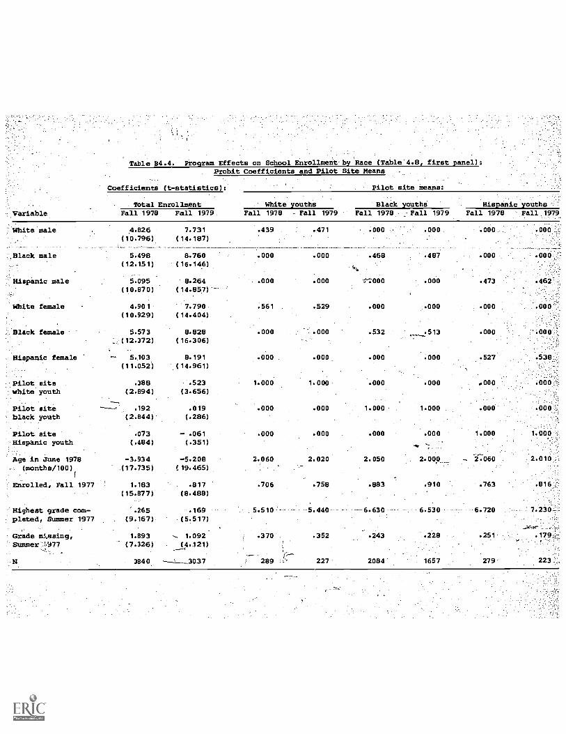
Table 84.4. Program Effects on School Enrollment by Race (Table 4.8, first panel):Probit Coefficients and Pilot Site Means


Total Enrollment White youths Black youthsVariable Fall 1978 Fall 1979 Fall 1978 Fall 1979 Fall 1978

White male 4.826 7.731 .439 .471 .000

(10.796) (14.187)

.Black male 5.498 8.760 .000 .000 .468(12.151) (16.146)

Hispanic male 5.095 8.264 .000 .000 :n000(10.870) (14.857)

White female 4.90 1 7.790 .561 .529 .000

(10.929) (14.404)

:.Black female 5.573 8.828 .000 .000 .532(12.372) (16.306)

Hispanic female 5.103 8.191 .000 . .000 .000

(11.052) (14.961)

Pilot sits .388 .523 1.000 1.000 .000

white youth (2.894) (3.656)

Pilot site .192 .019 .000 .000 1.000

black youth (2.844) (.286)

Pilot site .073 - .061 .000 .000 .000

Hispanic youth (.484) (.351)

Age in June 1978 -3.934 -5.208 2.060 2.020 2.050(months/100) (17.735) (19.465)

Enrolled, Fall 1977 1.183 .817 .706 .758 .883

(15.877) (8.488)

Highest grade com- .265 .169 5.510 5.440 6.630

plated, Summer. 1977 (9.167) (5.517)

, .

Grade m!,,esing, 1.893 .. 1.092 .370 .352 .243

Summer -1477 (7.326) (4.121)

I-3840 3037 289 ' 227 2084

Hispanic youths,.:Fall 1979 Fall 1978 Fall.1979

.000 .000 . .000

.487 .000 , .000

.000 .473 .462

.000 .000 .000'

.513 .000 -.000:':-. ,-

..000 .527 .538 ..,..,

.000 .000

1.000 .000 .000 ,-

.000 1.000 1.000

2.000 -. 2.060 2.010

.910 .763 .816,

6.530 -6.720 7.230

.228 .251

1657 279' 223

Variable

Table B4.5. Program Effects on Dropout Rates by -Race (Table 4.8,. second panel):Probit Coefficients and Pilot Site Means

Coefficients (t-statistics):

forin

Fall .1976 Fall 1979

Pilot site means:

White youthsenrolled inprevious fall

Fall 1978 Fall 1979

Black, youths Hispanic youthsenrolled in enrolled inprevious fall previous fall

Fall 1978 , Fall 1979 Fall 1978 Fall 1979

White male

7k'ack-maie

.Hispanic male

White female

Black female

,Hlipanic female .

-Pilot sitewhite youth

Pilot site,black youth

Pilot siteHispan.tm youth

Agerfirl June 1978' (months/100)

,Highest grade com-pleted, Summer 1977

Grade missing,rSumier1977

6.402 8.022 .461 .481 .000 .000 : 600.(13.941) (12.768)

T.000-L=7.210 8.781 .000- ----.000 --------.476 .481 .000(15.658) (14.103)

6.833 8.496 .000 .000 .000. .000 .488 .4671

(14.255) (13.050)

6.50 8.008 .539 .519 .000 .000 .000(14.204) (12.810)

7.265 8.811 '.000 .000. .524 .519 .000(15.794) (14.154)

6.838 8.309 .000 .000 .000. .000 - .512 ,.,.533':,

(14.426) (13.040)

.509 .283 ' 1.000 1.000 .000', .000 .000 '.000

(3.325) (1.480)

.165 - .029 .000 .000 1.000 1.000 .000

(2.263) (.363)

- .065 - .246 .000 .000 .000 .000 1.000 1.000

(.389). (1. 119)

-4.344 -4.563 2.010 1.960 2.030 . 1.980 2.020 1.980

(17.836) (13.498)

.306 .142 6.980. 6.640 7.070 7.010-- 7.400 7.740

(9.668) (3.960)

2.234 .896 .201' .211 .195 .175 .169 :117

(7.862) (2.864)

3228 2215 204 133 .; 180 1313 213 137.;.

Whis model predicts the school retention rate Which equals one minus the dropout rate.

2 51

Table B4.6. Program Effects on Return-to-School Rates by Race (Table 4.8, third panel):Probit Coefficients and Pilot Site Meant/

Coefficients (t-statistics): -Pilot site means:

Variable

Total enrollment for:youths not enrolledin previous fall

White youths.not enrolledin previous fall

Black youth's',

not enrolledin previous fall

-.-:Hispanic youthsnot enrolled in,:previous.fall

Fall 1978 Fall 1979' Fall 1978 Fall 1979.'' Fall 1978 Fall 1979 Fall 1978 Fall',1379

White male 2:839 3.407 .388 .457 .000 .000 .000 .000;

(2.334) (3.005)

Black male 2.700 4.573 .000 .000 .403 .512 .000 .000

(2.116) (4.145)

Hispanic male 2.310 4.081 .000 .000 .000 .000 .424 .453

(1.729) (3.746)

White female 2.624 3.671 .612 .543 .000 .000 .000 .000,

(2.066) (3.217)

Black female 2.884 4.689 .000 .000 .597 .488 .000 .000

(2.303) (4.239)

Hispanic female 2.360 4.344 .000 .000 .000 , ' .000 .576

(1.834) (4.029)

Pilot sitewhite youth

- .092(.282)

.607

(1.995)

1.000 1.000 .000 .000 .000 .000.,

Pilot siteblack youth

.392

(2.155)

- .084

(.564)

.000 .000 1.000 1.000 .000 ..000,

Pilot site .639 .173 .000 .000 .000 .000 1.000 1.000,'

Hispanic youth (1.677) (.536)

Age in June 1978 -1.969 -2.517 2.190 2.100 2.190 2.09P 2.190- 2.070:

(month6/100) (3.471) (4.435)

Highest grade com- .061 - .030 2.000 3.740 3.280 4.680 4.530 6.420

pleted, Summer 1977 (.771) (.431)

Grade missing, .186 - .343 .776 .553 .609 .430 .515 .279

Summer 1977' (.266) (.565)

N 612 822 85 94 243 344 66

Program Effects on School Enrollment by Sex (Table 4.9,Probit Coefficients and Pilot Site Means

Coefficients (tstatistics):

Variable

'Uthite male

TotalinrollmentFall 1978 Fall 1979

4.927

(11.605)

first panel):

Pilot site means:

8.049(14.802)

Black male 5.499 8.811

(12.179) (16.239)

Hispanic male

White female .

Black female

Hispanic female

5.013 8.257

(10.941) _ _.(14.981)

4.973 7.971(11.094) (14.832)

5.532 8.690

(12.276) (16.110)

4.977 7.992(11.030) (14.786)

.179 - .048(2.240) (.593)

Pilot sitemale youth

Pilot sitefeMale youth

.241

(3.102)

.216

Males FemalesFall 1978 .Fall 1979 Fall 1978 . Fall 1979:

(2.730).

Age in June 1978 -3.938

(months/100) (17.780)

Enrolled, Fall 1977 1.184

(15.896)

Highest grade com- .266

pleted, Summer 1977 (9.227)

Grade missing,Summer 1977

1.911

(7.407)

-5.217(19.530)

.815(8.459)

.170

(5.576)

(4.203)

.3840 3037

.103 .105 .000 .000

.790 .794 .000 .000

.107,

..101 .000 .000 .,

.000 .000 .114 .110

..000 .000 .782 .780

.000 .000 .104 . .110

1.000 1.000 .000 .000

.000 .000 1.000 1.000

2.950 ,_2.010 2.000

.871 .902 `'7'.834 .867

6.430 6.370 6.590 6.590 -_-, - _

.258 .242 .259 .231

1234 1017 1418 1090

Variable

Table 84.8. Program Effects on Dropout Rates by Sex-(Table 4.9, second panel): -`


Coefficientn.(t-statistics): --.' Pilot site means:

Total enrollment for .: Male:youths .Female youths:

youths enrollSd in enrolled in enrolled in .-

previous. .. _.._

previous fall ,previous fall- .,e.fallt777Fall 1978 Fall 1979 Fall 1978 - Fall 1979 :Fa11,1978 :- Fall 1979, ;.

White male

Black male

Hispanic male

White female

Black female

1

Hispanic female

Pilot sitemale youth

Pilot sitefemale youth

Age in June 1978(months/100)

Highest grade com-_-__pleted,..Summer2.1977


N

6.531 8.350 .087 084 A .000

(14.296) (13.326)

7.162 8.933 .816 .831 .080 .000

(15.686 (14.266)

6.625 8.488 .097 .084 .000 .000

(14.281) (13.319)

6.641 8.137 .000 .000 .093 .084

(14.566 (13.154)

7.210 8.731 .000 .000 .815

(15.714) (14.079)

6.621 8.064 .000 .000 .092 .089 '

(14.361) (12.954)

.187 - .172 1.000 1.000 .000 .000

(2.128) (1.716)

.202 .146 .000 .000 1.000 1.000

(2.395) (1.492)

-4.340 -4.583 2.030 1.980 2.020 1.980

(17.920) (13.584)

.308 .141 6.880 6.850 7.290 7.220_(9.762) (3.926)

2.258 .900 .206 .187 .182

(7.976) (2.879)

3228 2215 1075 759 1183

--1This mciel predicts the school retention rate which equals one minus the drOpout rate.

2 4

Table B4.9. Program'Effects on Return-to-School Rates by Sex (Table 4.9, third panel):t

Variable

Coefficients


site Means:(t-statistics): PilotTotal enrollment foryouths not enrolledin previous fall

Male youths Female youths ..-,

not enrolled not enrolled in..:..

in previous fall previous fall`

Fall 1978 Fall 1979 Fall 1978 Fall 1979 Fall 1978, Fall 1979

White male 2.639 3.582 .208 .167 .000

(2.210) (3.241)

Bleak male 2.814 4.358 .616 .682 .000 .000

---(2.239) (4.012)

Hispanic male 2.613 '4.402 .176 .151 - .000 .000

(2.017) (3.684)

White female 2.341 3.756 .000 .000 .221

(1.885) (3.389)

Black female 2.825 4.349 .000 ,.000 .617 .632

(2.303) (4.018)

Hispanic feMale 2.495 4.174 .000 .000 .162 .177,

(2.028) (3.878)

Pilot site .159 .040 1.000 1.000 .000 .000

male youth (.751) (.217)

Pilot site .394 .145 .000 .000 1.000 1.000-,.

femae.youth (1.878) (.895)

Age'in June 1978 -1.936 -2.479 2.190 2.090 2.190 2.080

(months /100) (3.451) (4.472)

Highest grade com- .060 - .017 3.400 4.970 3.090 4.630

pleted, Summer 1977 (.763) (.252)

Grade missing, .162 - .238 .610 .403 .643 .451

Summer 1977 (.230) (.396)

612 822 159 258 235

JJ

'it

S

-Table 84.10. Program Effects on Enrollment, Dropout and Return -to- School Ratesfor the 15-16 Year Old Cohort (Table 4.5):Probit Coefficients and Pilot Site Means

Coefficients it-statistics):

Totalenrollment

Fall Fall

Tatal enrollmentfor youths en-rolled in Rre-vious fallFall Fall

Pilot cite means:

'natal enrollmentfor youths notenrolled 1.9 pre-

vious fall All youthsFall Fall Fall Fall

Variable 1978 1979 1978 1979 1978 1979 1978 1979

4);Constant .tv4. 6.958 8.951 8.083 8.640 18.06 8.664 1.000 1.000

(4.584) (8.196) (5.268) (6.888) (2.473) (2.665)Lt.

Pilot site .240 .119 .200 - .023 1.343 .434 1.000 1.000

(2.760) (1.631) (2.238) (.279) (2.553) (1.936)

Age in June 1978 -5.556 -6.088 -5.371 -5.067 -12.40 -4.991 1.940 1.930

(months/100) (6.931) (10.77) (6.509) (7.378) (2.982) (3.053)

White male - .49B - .666 - .591 - .540 .049 .049

(3.319) (4.889) (3.716) (3.483)

Black male 0.000 0.000 0.000 0.000 .370 .383

(-) (7) (-)

Hispenj.c male - .551 - .573 - .529 - .483 .041 -.042

0.080) (3.924) (2.941) (2.796)

White female - .477 - .66? - 4496 - .497 .057 . .056

(3.120) (4.917) (1.164) (3.026)

Black female -.102 .063 .082 - .001 .426 .412

(.994) (.800) (.795) (.015)

Hispanic female - .689 - .607 .760 - .610 .057 .058

(4.417) (4.343) (4.625) (3.697)

Male 0.000 0.000

I-) (7),

Female .632 .243

(1.323) (1.263)

White .403 - .941

(.804) (3.263)

Black -- 0.000 0.000

-) ( -)

Hispanic -..421 -

(.713) (1.241)

Enrolled, 1.425 1.044 .962 .961

Fall 1977 (8.108) (5.765)

Highest grade--" .451 .323 .449 .280 .575 .025 6.990 6.780

completed, . (9.009) (8.099) (8.722) (6.144) (1.668) (.231)

--SuMmer 1977

Grade missing, 3.178 2.141 '3.172. 1.891 3.771 .173 .182

.SuMmer 1977, (7.739) (6.399) (7.497) (4.911) (1.415) (.231)._

2005' 1920 ' 1924 1644 276 1377 1322

Youths enrolledin previous fall

Youths not enrolledin previous fall

Fall Fall Fall Fall1978 1979 1978 1079

1.000 1.000 1.009 1.000 :

I.000- 1.000 1.000 1.000

1.940 1.930 1.980 1.950

.045 .046

.376 .384

.042 .040

.054 .049

.429 .430

.054. .051

This model predicts the school retention rate which equals one minus the dropout rate:

An additiverece/sex sp,cification was required :for Convergence'of the maximum likelihood estimator

.358 . .506

.642 .494

.302 .175

.547 .662

.151 .163

7.110 7.060 4.000 4.830

'.160' .156 .491 .367

1324 53 166

Variable

Constant

Pilot site

Age in June 1978imonthm/100)

White male

Black male

Hispanic male

White female

Black female

Bispanic female

Table 84.11. Cumulative Program Effects on School Enrollment Ratesfor the 15-16 Year Old Cohort (Tables 4.6 and A4.5):Divariate Probit Coefficients and Pilot Site Means


Youths enrolled Fall 1977 (N -1766) Youths not enrolled Fall 1977 (N.79)1 YouthsenrolledFall 1977(N -1214)

Youths notenrolledFall 1977(N.52)

Total enrollment Correlation''of errors

Total enrollment Correlationof errorsFall 1970 Fall 1979 Fall 1978 Fall 1979

9.232 11.35 3.014 23.03 14.00 - .130 1.000 1.000 ;

(6.028) (8.629) (3.594) (2.950) (1.219) (.078)

.184 :128 -1.729 2.000 .409 14.34 1.000 1.000(2;042) (1.622) (2.004) (1.744) (.658) (.120)

-5.032 -6.960 -15.47 - 8.01 1.935 1.977(7.102) (9.754) (3.478) (1.332)

- .590 - .600 .046(3.537) (4.707)

0.000( -)

0:000(-)

- .531 - .633(2.025)

...!...--

(4.142)

- .489 - .676137021) (4.449)

.061 .036(.593) (.426)

- .780 - .654(4.717) (4.234)

Male

resale

White

Black

Hispanic

Highest grade .417 .367completed, (7.762) (8.259)Summer 1977

Grade missing, 2.907 2.401Summer 1977 (6.632) (6.641)

1Because of the small sample size, a simpler, race/sex specification was required for convergence of the maximumlikelihood estimator.

.390

.044

.052

.411

0.000

(-) .

0.000

(-)

.234 .096

(.404) (.970)

.120 - .766(.181) (.783)

0.000 0.000(-) (-)

- .352 - .359(.444) (.579)

4.308 - .138

(1.206) (.069)

Variable

Table 84.12.' Program Effects on Enrollment, Dropout and Return-to-School Rates for the15-16 Year Old Cohort, Excluding the Denver and Phoenix Sites (Table A4.4):

Probit Coefficients and Pilot Bite Means '.

Coefficientsit-statiatico):

Total enrollmentfor.youths'en-

TOtal'. rolledlenrollment :wious fall

Fall .. Fall Fall , Fall

1978 '1979. 1978 .11979

Total' enrollmentfor youths notenrolled in,pre-

Lwious fallFall Fall1979 . 1979

Pilot site means:

All youthsFall Fall1978 1979 ,

Youths enrolledin previous fall

Fall Fall1978

Constant

Pilot. site

Age in June 1978(months/100)

White male - .529(3.273)

Black male 0.000 .

I-)

White female .536(3.353)

Black female .123

(1.179)

Male

Female

White

Black

8.589 8.796 10:165 8.697

(5.104)

. 223

(2.308)

-6.262(7.123)

Enrolled,Fall 1977

Highest gradecompleted,Summer 1977


1:497(7.342)

(7.190) (6.031) (6.300)

.123 . .195 -`.016

(1.481) (1.964), (.172)

-6.106(9.930)

-6.294 - 5.192,

(6.990) (6.928)

- .762 - .637 .602

(4.947) (3.654) (3.371)

0.000 0.000 0.000

(-) (-) (-)

-'.720(4.910)

.054(.663)

1.190

(5.462)

- .580(3.514)

.103

(.975)

- .529(2.900).

- .023(.246)

. 411 .330 .414 .305 .

(7.749) (7.759) (7.622) (6.298)

11.418 6.502(13.442) (1.836)

1.160 .481

(1.634) (1.828)

-8.775 -4.062(1.896) (2.293)

0.000 0.000

. (-)

-.560 ..220

,(.904) (1.031).

.420(.669)

0.000

'.516(1.384)

-1.046(3.159)

0.000

.070

(.578)

2.756

(6.377)2.147 2.783 2.070

(6.053) (6.272) (5.083)

1655 1591 . 1593 1365

3.368(1.177)

62

::102

(.106)

1.000 1.000 1.000

1.0001.000 1.000

1.940

. 045 .045 .041

.427 .417

.054 .050

.489 .474 .492

1.940 1.930

.411

. 055

. 963 .962

6.820 6.590

.188 .199 .174

226 1127 1085 1085

. .

Youths.not enrolls,th:previous fall

Fall

1979 1979'

1.000 '.000 1.000

1.000 1.000 1.000

1.930 ' 1.980 1.960

.041

.424

.044

.491

-,

6.950 .6.910

. 405 .522

'.595 .478

. 357 .199

. 643 ':801.

3.430 4.350

.168 .548 . .419

949 42 136

This model predicts the school retention rate which equals one minus the dropout rate...

2An additive race /sex specification was required for convergence of the maXlmum likelihood estimator.

Table 850. 7rogram Effects on Employment Ratios. Separately by Period (Table 5.3):OLS Coefficients and Pilot Site Means

Tall .

1978

Coefficients (t- statistics!:

Constant -1225.36(-7.99)

Pilot dummy 21.13(14.63)

White male 6.74(2.31)

Black male 0.00

(-)

Hispanic male 7.82

(2.44)

Spring Fall' 1979 1979

-1056.00 -75.69

(-5.98) (-0.30)

23.05 15.43

(15.52)

8.45 4.98(2.81) (1.48)

0.00 0.00( -)

13.95(4.20)

(-1

12.84

(3.42)

White female -..... 4.68 6.40 - 6.77(-1.74) (-2.10)

Black female - 2.46 - 1.49 C:. - 6.22(-1.60) (-0.95) -,, (-3.47)

Hispanic female - 3.40(-1.12)

Age (months) 11.66(7.91)

Agm squared . - 0.03(-7.71)

Employment ratio, 0.04Spring 1977 (1.09)

Employment ratio,Summer 1977

Employment ratio.Fall 1977

R2

N

0.08(3.87)

(1.83)

.094

3840

- 1.71 - 8.87(-0.54) (-2.51)

10.25 1.08.-

(5.98) (0.44)

- 0.02(-5.89)

0.03(0.80)

0.10144,2)

qa.40)

- 0.00(-0.48),

- 0.04(-0.87)

0.06(2.46)

0.11

(2.98)

Spring Sommer Summer Summer1980 1978 1979 .1980

-392.25 -627.69 -631.82 -170.47(-1.32) (-3.47) (-2.83) (-0.95)

15.73 14.60 10.79 10.09(9.00) (9.44) (6.67) (5.32)

6.95 3.46 2.06 5.16(1.97) (1.11) (0.61) (1.37)

0.00 0.00 0.00 0.00( -) ( -) ( - )

11.42 8.94 8.07 9.11(2.98) (2.60) (2.27) (2.23)

- 5.86 - 10.18 - 15.97 . -4.22(-1.76) (-3.57) (-5.19) (-1.16)

- 5.81 - 4.11 - 7.04 .9.46(-3.15) (-2.48) (-4.14) (-4.76)

- - 7.69 - 1.23 - 7.95 -10.25(-2.11) (-0.36) (-2.35) (-2.72)

4.34 6.16 6.61 4.23(1.47) (3.60) (3.02) (1.08)

0.01 - 0.01 - 0.02 -0.01(-1.53) (-3.60) (-3.04) (-1.12)

0.01 - 0.04 - 0.05 0.03( -0.30) (-1.06) (-1.09) (0.67)

0.08 0.18 0.09 0.07(3.10) (7.90) (4.00) (2.60)

0.08 0.05 0.07 0.06(2.11) (1.58) . (2.10) (1.51)

.100 .050 . .050 .067 .043 .041....._--

3759 3037 2890 3428 3377 2403

Pilot Site Means:

Whitamele .048

Black male .369

Hispanic male. . .U50

White female .061

Black femeln .418

.055

,204.87

42154.15

8.84

Hispanic female

.048 .051 .048 .048

. 372 .383 .383 .365

.049 .050 .Oil

.0v.i.'' .057 .056 .063--' -

614:. .403 .406, .420'

. 053-- .057 .057 .053

201'.62 200.59 199.48 207.99

41624.92 40362.37 39901.23 43429.01

6.42 5.64 5.31 7.78

.048

Employment ratio,.Summer 1977

Employment ratio,Fall 1977

22.76

10.53

2652

22.69

9.94

21.,07

9.00 8.36

.2107 2000

23.91

11.92

.048 .047

.775 .781..

.050 .052

.057 .053

.398

.063

197.99

39282.7,1

21.46

.414

.056

202.14

41001.52

6.03

2353

Table 85.2. Program Effect, on Employment Ratios, Separately by Period for Denver/Phoenix (Table 5.5)i77

OLS Coefficients and Pilot Site Means

Tall

1978..

Spring1979

Tall1979

Spring'1980

Summer1978

Summer1979

Summer1980


Constant -466.82 -294.04 116.19 -727.64 -149.90 -438.49 723.31 ,.

(-1.28) (-0.68) (-0.17) A-0.88) (-0.33) (-0.79) (-0.66)

--,__

Pilot dummy 9.01 5.71 -2.00 .. 3.10 11.74 - 0.39 8.68

(2.43) (1.53) (-0.47) 4-0.69) -(2.08) (-0.10) (1.76)

White male 13.92 18.72 18.91 20.76 11.98 5.13 15.18

(1.82) (2.46) (2.28) (2.32) (1.48) (0.64) (1.37)

Black male 0.00 0.00 0.00 0.00 ,0.00 0.0C 0.00

(-1 (-1 (-1 ( -1 ( -) (-) e-)

Hispanic male 9.85 20.02 22.88 21.09 10.73 11.95 19.86

(1.81). (3.68) (3.82) (3.40), (1.84) (2.08) (3.03)

White female 3.11 10.31 6.76 9.83 - 1.64 2.62 1.92

(0.43) (1.42) (0.74) (1.12) (-0.22) (0.33) (0.20)

Black female - 3.42 0.38 3.33 3.69 - 2.58 - 4.01 0.69

(-0.54) (0.06) (0.46) (0.49) (-0.38) . (-0.59) (0.09)

Hispanic female - 1.80 4.45 2.50 2.27 - 0.66 - 4.97 0.60

(-0.34) (0.83) (0.42) (0.37) (-0.11) (-0.88) (0.09)

Age (months) 4.46 3.02 - 1.00 7.32 1.81 4.72 - 7.00

(1.27) (0.72) (-0.15) (0.89) (0.42) (0.87) ( -0.64)

Age squared - 0.01 - 0.01 0.00 - 0.02 - 0.00 - 0.01 0.02

(-1.20) (-0.71) (0.16) (-0.87) (-0.46) (-0.88) (0.63)

Employment ratio, 0.13 0.05 0.01 - 0.02 0.02 0.00 0.08

Spring 1977 (1.94) (0.78) (0.16) (-0.20) (0.22) (0.03) (0.88)

Empleyilent ratio, 0.11 0.17 0.20 0.20 0.16 0.11 0.15'

Summer 1977 (2.16) (3.57) (3.72) ,(3.59) (3.21), (2.12) (2.49)

Employment ratio, - 0.02 0.14 0.10 0.02 0.03 0.13 0.06

Tall 1977 -(0.30) (2.35) (1.39) (0.28)' (0.51) (2.00) (0.81)

.- 112

H

.070 .110 .103 .082 .071 ..059 .086 -

654 626 506 485 578 571 418

Pilot Site Means:

White melt . .063. .066 .070 .061 .069 .068 7--.--.053---=

..__

0ieck male .162 .167 .169 .175 .160 .163

Hispanic male .261 '.261 .261 .263 .259 .259 .257

White female .076 ', .075 .065 .067 .085 .075 .060

Black lemale..- .145 .139 .124 .134 .150 .139 .135

Hispanic female"',` .293 .292 .306 .300 .277 -.296

Age (months) 205.45:' 203.89 201.13 ,.-. 200.36 207.99 202.59

Age squared 42398.93 41729.53 40565.17 . 40242.19 43438.89 41172.81 .,39566.57.`

Employment ratio, 12.42 11.62 '10.60 .,l9.86 13.76 11.07

. Spring 1977

Employment ratio, ,35.50 35.53

Summer 1977

Employment ratio, 19.20 18.10

Fall 1977

34.65 t.

475 462 372 357 433

Table 85.3. Program Effects on Employment Ratios, Separately by Period, for Cincinnati/Louisville (Table 5.5):OLS Coefficients and Pilot Site Means

Coefficients

Constant

Pilot dummy

White male

Black male

Hispanic male

White female

Black female

Hispanic female

Age (months)

Age squared

Employment ratio,Spring 1977


'Employment ratio,Fall 1977

R2

Frill-1978

Spring1979

Fall1979

Spring1980

Summr11974

Summer197 9

Summer,

1980

(t-statistics):

-841.38 -1114.02 -318.26 -508.66 -223.27 -862.60 367.64(-3.13) (-3.50) (-0.74) (-0.96) (-0.73) (-2.12) (0.51)

15.87 18.00 17.13 16.55 10.70 , 9.08 - 11.05

(6.49) --', (6.99) (6.06) (5.56) (4.13) (3.17) (3.28)

1.60 0.77 3.76 1.65 . 4.78 - 2.16 1.43

(0.37) (0.17) (0.74) (0.30) (1.05) (-0.42) (0.24)

0.00 0.00 0.00 0.00 0.00 0.00 0.00

(-) ( -) ( -) (-) (-) ( -) (-)

- 29.98 - 8.91 .0.88 - 18.69 - 26.90 7.13 - 31.66

(-1.34) (-0.39) (0.04) (-0.78) (-1.20) (0.29) (-1.07)

- 5.94 - 8.72 - 2.89 - 4.94 - 10.82 - 14.45 - 1.72(-1.52) (-2.11) (-0.65) (-1.04! (-2.64) (-3.17) ( -0.33)

- 4.89 - 6.84 - 12.37 - 11.34 - 6.68 - 12.01 - 7.58

(-1.80) (-2.41) (-3.99) (-3.47) (-2.32) ( -3.84) (-2.11)

- 1.49 0.74 - 3.11 0.08 22.60 11.39 - 5.06

(-0.08) (0.04) (-0.13) (0.00) (0.82) (0.54) (-0.21)

8.10 - 10.84 3.32 5.47 2.25 8.69 -. 3.08

(3:14) (3.51) (0.78) (1.04) (0.78) (2.18) (-0.42)

- 0.02 - 0.03 - 0.01 - 0.01 0.01 - 0.02 0.01

(-3.09) (-3.46) . (-0.77) (-1.07) (-0.77) (-2.16) (0.38)

0.11 0.03 - 0.01 0.01 0.01 - 0.07 0.03

(1.92) (0.44) (-0.10) (0.10) (0.24) (-0.91) (0.31)

0.12 0.15 - 0.00 0.04 0.15 0.08 - 0.01

(3.10) (3.83) (-0.08) (0.84) (3.86) (1.81) (-0.14)

0.06 0.11 0.16 0.14 0.05 0.11 0.18

(t.24) (2.05) (2.58) (2.04) (0.94) (1.75) (2.32)

.100 -- .116 .075 .072 .075 .053 .046

N 1085 1054 881 833 976 957 711

Pilot Site Means:

White male .064

Black male .369

Hispanic male .003

ral".,,Jamale .099

aitc'famale .460


Age (months) 204.60

Age squared 42038.94

.465 p065

.372 .390

.003 - .004

.094 .f&"

.461 .441

.005 . .004

.203:77 200.84

41681.76' 40468.90

Ltployment ratio, 9.08 8.93 7.92

Spring 1977

Employment ratio, 26.38 26.71',

summer 1977

Employment ratio, 12.42 12.17Fall 1977

N

.059

.393

.004

.092

.062 .062 .056

.370 .385 .400

.003 .003 .002

.099 .093 .089

.464 .452 .449

.002 .005 .004

13.18 202.33 198.10

41077.84 39331.57

8.18 7.107.88

24.08 28.45 25.35

658 649

Table B5.4. Program Effects on Employment Ratios, Period, for Baltimore/Cleveland (Table 5.5)z

OLS EoerficCoefficient, AaA Pilot Site Means

Coefficients

Constant

Pilot dummy

White male

Black malt

Hispanic male

White female

Black female

Hispanic female

Age (month)

Age squared



Employment iatio,Fall 1977

Pall

1978

Spring1979

rill1979

.

".ring.1980

(t-statistics):

-2047.82 -1442.51 70.09 -627.12

(-7.42) (-4.65) (0.16) (-1.25)

27.17 32.44 19.07 19.11

(9.27) (10.85) (5.64) (5.54)

0.10 7.58 11.68 13.22

(0.01) (1.03) (1.47) (1.64)

0.00 0.00 0.00 0.00

(-) ( - ) ( -) ( - )

fr

- - 0.71 4.01 2.26

(-0.28)' (-0.05) (0.24) (0.13)

- 5.65 - 11.48 - 9.99 - 6.25

(-0.84) (-1.66) (-1.29) (-0.78)

0.45 3.54 - 2.75 - 3.24

(0.18) (1.38) (-0.94) (-1.09)

- 7.41 4.66 - 14.28 ,- 23.01

(-0.48) (-0.28) (-0.84) (-1.25)

19.54 14.03 0.03 7.08

(7.37) (4.66) (0.01) (1.42)

- 0.05 - 0.03 - 0.00 - 0.02

(-7.24) (-4.61) (-0.11) (-1.53)

- 0.09 0.03 - 0.14 0.09

(-1.28) (0.40) (-1.51) (-0.:9)

0.05 . 0.03 0.05 0.05

(1.33) (0.88) (1.20) (1.01)

0.06 0.06 0.11 0.14

(1.12) (0.97) (1.60) (1.88)

R2 -.114 .110 .048 .053'

N 1299 1279 1037 992

-1699.10"(-5.32)

-385.31(- 1.02).

- 1167.86..

(-1.86)

13.80(4.45)

- 6.08

'12.23

. (3.99)

8.81

7.97(2.29)

4.14

(-0.79) (1.16) ' (0.51)

0.00 3 0.00

(-) (-) (-)

- 3.76 - 20.91 5.66

(-0.26): (-1.35) (0.34)

- 9.67 - 27.64 3.51

(-1.35) (-3.77) (0.43)

- 0.57

(-0.21) (-0.85) (-3.20)

4.36 - 20.75

(0.24) (-0.19) (-1.06)

16.51 4.55 12.58

(5.47) (1.23) (1.99)

- 0.04 - 0.01 - .0.03

(-5.52) (-1.34) (-2.05)

- 0.01 - 0.10 - 0.03

(-0.13) (-1.23) (-0.30)

0.18 0.09 0.06

(4.42) (2.35) (1.25)

0.02 0.08 0.04

(0.43) (0.91) "(0.44)-

Pilot Site Means:

--White male' 019 018 - -- 023 .022

Black male 2

Hispanic male .006

.421

.006

.433

.005

.436

.005

.028White female .027 .029 .029


.520

.004 .005 .005

. Black female .524 .505 .503

Age (months) - 205.42 203.95 200.53 199.50

.063

1170

.043

1204

.032

884

.020

.421

.007

.028

.521

.003

208.76

.019

.400202255

.525

.004

202.61

.023

.430

.027

.509

.005

197,f2.

Age squared , 42387.41 41765.09 40343.86. 39912.53 43757.43 41193.20 39138.56'

Employment ratio, 4.25 '3.82 3.19 2.97 4.72 3.70

Spring 1977

Employment ratio, 19.79 19.68 17.27 17.03 20.60

Summer 1977

Employment ratio, 7.70 .'5.36

fall 1977

759

Program Effects on Employment Ratios, Separately by Period, for Mississippi Pilot /Control

Fall1978

Spring1979

01.5 Coefficients and Pilot Site Means

Summer.1979

Fall1979

Spring1980

Summar1978


Constant -1172.22 -953.43 -526.28 -110.53 431.92 -849.57

(-3.50) -2.60) (-1.00) (-0.17) (1.03) (-1.68)

Pilot dummy 19.79 20.96 13.61 16.14 11.82 12.31

(6.95) (7.20) (3.82) (4.42) (3.76) (3.64)

. . . . . .. . . .

White male 21.18 21.87 1.40 9.20 12.36 8.05

(3.66) (3.67) (0.19) (1.25) .(1.90) (1.14)

Black me), 0.00 0.00 0.00 0.00 0.00 0.00

( -) ( -) ( -) ( -) ( -) ( -)

White female - 1.80 - 7.68 - 13.55 - 14.39 - 4.63 - 23.85(-0.66) (-1.30) (-1.77) (-1.77) (-0.72) (-3.22)

Black female - 6.16 - 6.52 - 9.86 -8.39 8.85 - 13.32

(-2.13) (-2.20) (-2.74) (-2.28) (-2.77) (-3.85)

Age (months) 10.99 9.00 5.21 1.10 - 4.27 8.32

(3.40) (2.52) (1.00) : (0.17) (-1.07) (1.67)

Age squared - 0.03 - 8,02 - 0.01 - 0.00 0.01 - 0.02

(-3.25) ( -2.40) (-0.95) (-0.13) (1.17) (-1.59)

Employment ratio, - 0.09 - 0.07 - 0.01 0.1S - 0.26 0.02

Spring 1977 (-0.93)

employment ratio, 0.03

.. (-0.72)

0.06

(-0.06)

0.01

(0.98)

0.04

. (-2.59).,

0.15

(0.15)

0.08

Summer 1977 (0.54) (1.18) (0.23) (0.56) (2.83) (1.29)

Employment ratio, ' 0.15 0.08 0.05 -- 0.01 0.13 - 0.10Fall 1977 (1.99) (1.00) (0.44). (-0.06) (1.54) ( -1.08)

R2 .129 .120 .050 .064 .080 .079.

N t02 800 03 580 704 . 645.

Pilot Site Means,

.070 .072 .072 .067 . .071White male .070

Black male .448 .455 .472 '.469 .445 .476

White female .064 .064.. .058 .051 .065 .056

Black female .418 .411 .398 ' .408 .423 .397

Age (months) 203.63 202.57 199.86 - 198.58 206.22 200.38

,. ',-

Age squared 41623.83 41178.28 40066.44 39536.31 42664.78 40281.12

Employment ratio, 3.88 .3.70 '2.79 2.23 4.25 .14

Spring 1977

Employment ratio, 12.30 12.10 10.70 9.58 12.39 11.27

Summer 1977

Employment ratio, 5.65 5.28 4.85 4.27 6,12 5.16

Fall 1977

(Table 5.5):

Summer'1980

-874.65(-1.00)

9.59'(2.24)

15.33(1.87)

0.00

( -)

- 13.42

(-1.32),

- 17.75(-4.02)

8.61.

(0.98)

- 0.02

(-0.91)

.0.07(0.39)

0.11

(1.55)

- 0.08(-0.68)

'.087

--. -.523

.046

.344

197.80

39218-85

'2.23

11.53

5.11

241516 400

Table-h5.6. Program Effects on Employment Ratios of Private Sector Employment Ratios (Table 5.6):

OLS Coefficients and Pilot Site Means,

Fall Spring Fall Spring Summer Summer Summer

1978 1979 . 1979 1980 ' 1978 1979 1980

Coefficients (t-statistic.):

Constant .-389.03,-1(-3.28) ( -1.02)

108.09 -108.95

(0.51)1 (-0.43)


3.22. 0.93

White male

(3.22) (2.24)

'(:1!.649119)

(5.73) (4.63)

(0.77)

13.02 15.05 .12.41

(6.30) (4.33) (5.64)

Black male - 0.00 0.00 o.no 0.00 o.00

(-) (-) (-) (-) .(-)

15.63 18.89 18.83

---..

Hispanic male2(7.18) (6.33)

18.39

(6.23) (5.75)

White female 4.24(2.06) (1.20)

2.64(0.15)

1.09

)

1.11

(6.92)

(0.39)

Black female . - 4.33 - 5.08(-4.09) -(-::::)

- 10.07 -

(0.50)

(-3.65) (-6:40) ( -3.45)

Hispanic female 0.88 2.61 2.78 1.49

(0.37) (1.04) (-0.5 57

-.

( -0.52) (-0.89) (0.57)

-182).48.

(-1.31)

Age (months) 3.60

(3.15)

Age squared - 0.01

(-2.93)

Private sector. 0.05

employment ratio, (1.61)

Spring 1977

Private sector 0.05

employment ratio, (2.30)

Summer 1977

sector 0.16

an4,4tyment ratio, (6.06)

fall 1977

R2

1.27

(0.94)

- 0.00

(-0.76)

0.07(2.18)

0.03(1.42)

- 1.05

(-0.50)

0.00(0.58)

0.00(0.06)

0.05(1.69)

0.18 0.16

(6.44) (4.39)

1.15

(0.46)

- 0.00

(-0.40)

0.02

(0.51)

0.08(2.48)

0.14

(3.51)

1.68

(1.27)

- 0.00(-1.14)

- 0.02

(-0.61)

-30.69 -293.19

(-0.16) (-0.83)

- 0.09 4.32

(-0.07) (2.51)

14.68 15.27

(5.33) (4.46)

0.00 0.00( -) (-)

20.04 18.57

(6.72) (5.01)

- 1.07(-0.42)

- 8.95( -6.29)

- 0.28(-0.10)

0.31

(0.17)

- 0.00(-0.05)

- 0.02(-0.62)

0.10 0.05

(4.25) (1.77)

0.20(7.32)

0.17

(4.96)

.095 .097 .073 .075 .107 .078

3840 3759 3037 '2890 3428 3377 ,,,,.,.....,..2403

(1.26)

11.91

(- 6.63)

- 4.46( -1.31)

3.11

(0.88)

- 0.01

(-0.86)

0.09(2.49)

0.09(1.99)

White

Pilot Site Means:

male .048 .048 .051

Black male .368 .372 .383

Hispanic male .050 .048 .049

White female .061 .060 .057

Black female .418 .419 .403

Hispanic female tOSS .053 .057

Age (months) ---204.87 203.62 200.59

Age squared 42154.15 41621.92 40362.37,

Private sector 5.48 5.07_ 4.41

employment-ratio,Spring 1977

Private Sectoremployment ratio,Summer'1977

Private sectoremployment ratio,

' Pall 1977

10.62

7.72

10.35 9.76

7.16 6.66

.048 .048 .047

. 383 .365 .375 .387

.050 .051 .050 .052

. 056 .063 .057 . .:053

.406 .420 .414

. 057 .053 .056

199.48

39901.23

4.20

207.99

43429.01

6.24

9.26 11.35

6.18 8.77

202.14

41001.52

4.67

.063

197.99

39282.71

4.01

9.93 9.67

2652 2605 2107 2000 2353 2362

6.11

193 264

:1; t

Table B5.7. Program Effects on Employment Ratioc of Public Sector Employment Ratios (Table 5.6):OLS Coefficients and Pilot Site Means

Fall Spring Fall Spring Summer SUmmer Summer

1978 1979 1979 1980 1978. 1979 1980


Constant -840.30 -929.67(-6.74)


White male - 7.42(-3.15)

Black oars 0.00

(-)

Hispanic male - 8.77(-3.311

hhite female

Black female

Hispanic female

Age (months)

Age squared

Public sectoremployment ratio,Spring 1977

- 9.00

,( -6.32)

18.26(14.76)

- 7.55(-3.03)

0.00

(-)

- 5.33(-1.93)

- 214.79

(-1.17)

12.25(9.79)

- 8.67(-3.51)

0.00( - )

- 7.60(-2.75)

- 9.54 - 7.62(-4.11) (-4.11) (-3.21)

2.39(1.92) (2.79)

- 4.66" 4.67(-1.88) (-1.77)

9.15(6.41)

3.63 2.97

8.11(6.77)

- 0.02(-6.77)

- 0.01(-0.09)

Public sector 0.14employment ratio, (6.34)Summer 1977

Public sectoremployment ratio,Fall 1977

0.04(0.93)

- 0.02(-6.48)

- 0.06 ,

(-1.00)

0.11(4.73)

(2.26)

- 7.72

(-2.96)

2.44(1.34)

- 0.01(-1.49)

- 0.15(-2.31)

1.05(2.37)

0.12 0.05(2.63) (0.98)

-307.56 -480.62(-1.39) (-3.19)

12.12(9.29) (10:41)

- 8.39 - 11.92(-3.20) (-4.62)

0.00 0.00

( -)( -)

( -)

- 7.81(-2.74) (-3.75).

- 7.61 - 11.70(-3.06) (-4.91)

.4.42 0.72(3.22) (0.53)

- 5.29 - 3.20(-1.94) (-1.14)

'3.44 4.84(1.56) (3.40)

-625.31(-3.36)

10.77(7.98)

-87.51

(-0.3

5.4:

(4.2:

13.74 -11.0:(-5.08) (-4.0'

'0.00 0.01

- 0.01(-1.70)

- 0.06(-0.85)

0.04(1.88)

- 0.01(-3.54)

- 0.12(-1.89)

0.22.. (9.52),

- 12.42(-4.21)

- 15.11

(-5.88)

2.09(1.48)

- 8.

(-2.87)

( -

- 9.71

'( -3.3:

6.55

8.7(-3.3

2.6(1.8!

- 6.0:

(-2.2'

1.2:

.(3.59) (0.4,

- 0.02(-3.76) .:

- 0.12(-1.66)

7 0.01

(-0.5:

. 0 A:(0.6,

0.11 0.0,

(4.64) (1.71

0.02 0.04 0.08 0.0(1.53) (0.21(0.45) (0.98)

R2

.498 .096 .064 .065 .095 .072 .04

N 3840 3759 3037 _2890 3420 3377

Pilot Site Means:

White male .048

Black rale-- .368

Hispanic male '.050

White female

Black female

.061

.418

'Hispanic female .055

Aga (months) 204.87


Public sector 1.36employment ratio,Spring 1977

Public sectoremployment ratio,Summer 1977

Public sectoremployment ratio,Fall 1977

.048 .051 .048 .048

. 372 .383 .383. .365

.048 .049 .050 .051

. 060 .057 .056 .063

.419 .403 .406 .420

.053 '.057 .057 .053

203.62 200.59 199.48 207.99

41621.92 40362.37 39901.23 43429.01

1.35-7 1.23

.048

.375

.050

.057

.414

.056

. 64'

. 38'

.051

. 05:

. 391

..06:

197.91

.39282.7'

1.0:

TADLO 172.42. rrogram recta on &mpioymeni nmmion, popeznmsay .7 ..+,.

Tall Spring1979

OLS Coefficients and Pilot Sits means

Summer1979

, Tall1979

Spring-1980 1978

Coefficients ft-utt:mica):

Constant -1005.07 -617.80 .4783.15 -261.21 168.93 -299.54

( -1.55) (-0.81) (-1.58) (-0.18) (.0.22) (.0.32)

Pilot chimp 16.63 12.29 3.62 15.06

(2.99) (2.14) (0.57) (2.33) (1.64) (.0.50)

,.,.

Age (months) 9.61 5.95 17.31 2.06 2.08 _

(1.54) (0.80) 4(1.57) (0.14) (0.29) (0.33)

Age sguasirct - 0.02 - 0.01 - 0.04 - 0.00 - 0.01

(-1.50) (-0.76) ( -1.52) 1 II) ( -0.32) (-0.30)

Employment ratio. - 0.09 - 0.01 - 0.03 -.09 - 0.16 . . 0.04

Spring 1977 '( -0.96) (- 0.06) ( -0.27) (.0.78) (.1.67) (0.35)

Employment ratio. 0.11 0.21 0.04 --,-. 0.28 0.15 0.06

Summer 1977 . (1.31) (2.33) (0.36( (2.76) (1.68) (0.63)

Employment ratio. 0.23. ..

0.11 0.22. 0.10 0.26 . 0.11._

Tall 1977 (2.62) (1.22) ,(2.12) (0.91) (2.88) : - (1.14)

.107 .098 .079 ..134 .081. , .042

239 232 194 178 217 . :206

'Pilot Site Means:

Age (months) 204.90 204.23 201.93 199.77 207.55 202.98

Age squared 42147.15. 41882.69 40921.65 40016.17 43244.03'. -41363.23


Spring 1977Employment ratio, 30.19 29.64 28.53 26.70 32.45 28.69

Summer 1977

:employment ratio, 21:61 26.99 22.39 18.99 24.73 22.52

Tall 1977

' 127 126 107. 96

114. 113

Summer.1980

761.75: (0.37)

6.45(0.90)

- 7.64

(-0.37)

0.02(4,39) '.

- 0.06

( -0.39)

0.19(1.67)

0.17:: (1.48)

, .077 .

149- ::

198.37.

'39433.787t_....

29.06

20.82'

Table 85.9. Program Effects on Employment 'Leos, Separately by Period, for Slack Males (Table 5.7):

Bummer1980

Tall1978

Spring1979

OLS Coofficientm and Pilot Site Moans.

Summer1979

Pall1979

Spring1980

SUMber.1978

Coefficients (t- etatietica),

Constant -1212.70 -1135.62 388.65 -195.86 - 415.02 -587.74 -605.818

(.4.51) (-3.76) (0.96) (-0.41) (-1.36) ( -1.57) ' (-0.97)

_Pilot dummy 22.60 25.41 18.92 19.72 14.54 11,12 10.45

(8.90) (9.84) (6.50) (6.61) (5.37) (4.05) 13.29)

Ago (months) 11.40 10.79 - 3.72 2.26 3.95 5.98 6.43

(4.40) - (3.68) ( -0.931 (0.48) (1.37) (1.64) (1.02)

Age squared - 0.03( -4.23)

..- 0:03 .-

(.3.54)

0.01 .

(0.95)

7-.7-0.01 ,

(- 0.49)

. 0.01(-1.29)

.0 01_

(- 1.60),

_ .

-

- 0 02. ..

(.1.02). 77-.

.

Employment ratio. 0.06 0.06 , - 0.07 - 0.12 - 0.00 - 0.12

Spring 1977 .' (1.07) (0.92) (-0.94) ( -1.55) . ( -0.04) ( -1.74).

( -1.27)

Employment ratio, 0.06 0.06 0.03 0.03 . 0.14 0.09 . 0.01

Summer 1977 (1.67) (1.77) . (0.70) (0.77) (3.88) .(2.51) .

(.0.16).

10Mployment ratio, 0.03 0.03 , 0.11 "-',2.14 ..: 0.02 0.07 0.18

Pall 1977 (0.57) (0.53) (1.64) (3.00) . ( -0.31) (1.26) : (2.43),-

62

.096 .100. .043 .045 .045 .026 021

1349 1331 1121 1067. 1208 1226 903

Pilot Site Means:

Age (months) -704.42 203.67 200.58 199.50: 208.07. c 202.09 197.76

Age squared 12048.72 41645.89 40359.41 39409.77' 13460.84 _ 40982.67 39192.77

Employment ratio, 8.19 6.74 6.56 9.19 7.3C 6.24

.Spring 1977

rmplOyment ratio. 28.02 27.65 24.89 24.17 29.33 26.45 .25.21

Summer 1977

Employment ratio, 11.81 ,- 11.14 9.04. 13.66 8.58

Fall 1977.,

975,

807.. 768. > 858C.

.'

887 '653

195

OLS Coefficients and Pilot Sits Means

Fall Spring. Spring &Eimer

1978 1979 1979, .1980 .'1978 1979 1980

Coefficients (t-statistics) s _.

Constant - 279.45 68.83 70.95 -1032.87 120.14 17.61 -.1056.41

(.0.30) (0.09) (0.05) (0.14) . (-0.02)

Pilot dummy 0.36 3.08 6.65 4.19 3.15 --: 1.60 13.69

(-0.05) (0.45) (0.82) A0.49) (0.44) ---, ( 4.22) ..(1.55)

Age (months) 2.50 0.67 - 0.05 10.88 - 0.95 0.46 11.69

(0.36) ( -0.09) 1-0.00) (0.68).

( -0.12) (0.05) (0.53) J.,

Age squared -. 0.00 0.00 0.00 - 0.03 0.00 - 0.00 0.03

( .-0.28) (0.14) (.0.02) ( -0.70) (0.14) (- 0.02) - (- 0.57)'

Employment ratio, 0.09 0.06 .. 0.03 - 0;03 . 0.06 0.06 . 0.08

Spring 1977 (0.71) . (0.53) (-0.23) (..0.19) ( -0.48) (-0.49) (0.56):

Employment ratio, 0.06 0.12 0.17 0.16 0.17 0.14 0.13

Summer 1977, , (0.67) (1.321 (1.59) (1.51) (1.80) (1.46) (1.23)

Employment ratio, - 0.05 I 0.07 0.10 - 0.02 0.02 0.08 0.00

Pall 1977 (..0.46) (0.65) .(0.70)..

(- 0.18).. (0.19) (0.73) (0.01)

R2 , .052 .067,, .037 .022 .035 .029 .054

9

.

188 148 144 169 160

Pilot Site mangs

Age (months) 207.77 206.03 --, 202.49

Age 'squared 43371.36 42623.95 41124.02

Employment ratio, 18.11 16.76 13.41

Spring 1977

EMploymeneratio, 39.49Summer 1977

Employment ratio, 24.16.

Pall 1977

132

30.89

21.83

126

36.70

20.46

103

202.14

40976.60

.12.54

209.84

44211.41

19.30

.204.25 199.76

41859.94 39992.08

14.65

35.64 42.10 38.17 ,

20.08 . 26.46 20.87:-

100 % 120 117

Table 85.11. Program Effects on Employment Ratios, Separately by Period, for White Females (Table 5.7)2OLS Coefficients and Pilot Site Man.

Fall-- Spring1978 1979

fall1979

Spring Sumer1980 1978

Summer Suter1979 : 1980

Coefficients (t-statistics)s

Constant -41.29(-0.08)

.506.66(-0.87)

916.55(1.13)

Pilot dummy 6.22 7.08 - 1.01

(1.34) (1.56) (-0.18)

'71(2::1:)

- 499.96

( -0.67)

-1329.28

71f12).1 (-0.97),

2.56 2.27

(0.43) (0.32)

Age (months) 0.50 5.06: - 8.92 2.75 1.01 5.17 14.24

(0.10) (0.91) (-1.12) (0.30) (0.18) (0.71) (1.03)

----- Age squared 7-- 0.00 0.01 .- 0.00 . 0.04_

(-0.08) ( -0.91) (1.13) (-0.33) . (.0.15) ( -0.72) (-1.06)

Employment ratio, 0.13 0.01 . 0.01 0.43 0.06 0.11 0.52

Spring 1977. (1.12) (0.10) (-0.05) (2.35) (0.56) (0.79) (2.35)

Employment ratio, - 0.10 - 0.05 0.01 0.14 0.06 0.10 0.09

Summer 1977 (-1.20) (.0-53) (0.10) (1.29) (0.71) ( -1.14) (-0.61)

Employment ratio, 0.27 0.7 0.26 - 0.21 0.26 0.38 0.03 .

Pall 1977 (2.67) (4.75) (1.70) (-1.22) (2.59) (3.19) (-0.17)

.064 .125 .034 .046 .094 .072 r .052

274 213 201 263 233 160

Pilot Site Roans,

Age (months) 207:13 205.86 201.98 . 200.52 210.00 : 203.91 . 197.64

Age squared 43108.31 42558.03 40940.10- 40327.84 44294.19 41728.63 39141.24

Employment ratio, 10.41 9.19 8.31 7.70 12.13 8.13 ,'6.18

Spring 1977 1

Employment ratio, 16.90 15.73 :15.92 14.51 18.47 15.96 .12.35

Summer 1977

Employment ratio, 12.94 .11.69 8.93 8.21 14.62 1 10.39 6.71

rail 1977 . '

162 155 120 148

196

TablM'15.12. Program Effects on Employment Ratios, Separately by Teriod,'


Pilot dummy

Age (months)

Age squared

'Employment ratio,Spring 1977


R2

Employment ratio,Pall 1977

.

N ./

for Black Tamales (Table 5.7)e

Tell

Coefficients (t -statistica):

Spring

1978 .1979

Constant -1551.24 -1272.28

( -6.62) C.4.671

27.71 30.04..

(12.48) (12.91)

14.84

(6.58)

0.04

(-6.50)

0.11(-1.28)

0.13(3.71)

Employment ratio, 0.03

Pall 1977

1568

pilot Site Keane,

Age (months) 204.48

Age squared : 41984.70

Employment ratio. 2.52

Spring 1977

Employment ratio. 15.16

Summer 1977

12.46

(4.71)

0.03

(-4.71)

- 0.11

(-1.24)

0.12(3.52)

0.06

(-0.52) (1.05).'

.121 .113

1542

203.08

41392.54

2.33 .

15.57

5.50 5.32

1109 1092

Tall Spring . . Summer Suser Summer

1979 1980 1978 1979 1980

-676.42( -1.73)

22.07(8.31)

7.24

(1.87)

0.02

(-1.98)

- 0.14

(-1.39)

0.07

(1.69)

0.03(0.52)

.06/

1192

-755.22(-1.61)

19.25 '

(6.98)

8.13

(1.74)

- 0.02

(.01.82)

- 0.03( -0.27)

-- 0.04

(1.03)

0.10

(1.39)

.055

-1180.40(-4.16)

19.76

(8.23)

11.51

(4.29)

- 0.03

(-4.26)

- 0.09( -1.08)

0.23(6.43)

0.03(-0.52)

.084

-849.37( -2.42)

17.03

(6.62)

(2.57)

0.02(-2.65)

0.17(-1.71) -

0.12':(2.17)

0.04(-0.56)

.047

( -0.00) *.

10.20

(2.33)

0.59(0.10)

-0.00(- 0.15) -,-

-0.01( -0.06)

0.10(2.12)

-0.03( -0.33) .

.020

9251140 1396 1362

.200.01

40125.23

2.07

199.01

39708.04

2.07

207.46

43200.34

2.86

201:67

40803.36

2.25

197.90

39248.67

1.69

14.13 14.14 15.66 15.72 14.89

4.80 4.45 6.23 5.17 4.72

850 811 989 978 671

Table 85.12. program Effects on Employment Ratios, Separately by Period, for Hispanic Towel's (Telble,5.7le


Pall Spring Tall ,'Spring Summar Summer Summer

1978 1979 1979 1980 1978 1979 1980

Coefficient, (t- statistics!,.

410.22

(-1.40)i27.73(0.11)

-203.14( -0.13) 711C.1.91.:).Constant -1217.14

(-2.27)-1101.01

Pilot dummy 14.41 '' 4.96-(21.213)

(-0.86).

25.47 5.86

(2.49) :11:::4(0.81)

ATP (onnths).(2.231

12.40 11.15 - 1.04(1.1125)

13.50)

6.92(0.89) A1.421

14.63

(-0.70)

gm Aquaria(-2.18) .(.t:9)

(-0.09)

-.0.00

(0.08) (.0.17) (-0.90) ( -1.47)


Spring 1977 (2.02)

0.12 0.05 0.09 0.14 0.11

(0.77) (0.24) (0.43) (0.86) (0.62)


Summer 1977 (1.96) (2.40) (2.85) (3.67) (2.06) (1.09)

Employment ratio, - 0.02 0.15 ' 0.03. .. 0.067 .. 0.03 0.09 - 0.09

. Tall 1977 (-0.20) (1.40) (0.24) ( -0.46) (-0.22) , (0.77) . (-0.65)

-382.98

12.24(1.60).

4.28(0.23)

(3.22)

R2

Pilot Site ?manse

Age (months) 204.41



Spring 1977

..145 .129 .069' .102 .128 .056 .145

210 200 169 160 175 184 145

Employment ratio,Summar. 1977

Employment ratio,Tall 1977

, .

202.30 . 200.52 199.16 207.94 281.64 198.47

41068.72 '40321.85 39757.55 42411.09 40789.28 39476.25

5.71 :4.57 7.64 3.66'

30.63 30.95 . '29.69 3026 23.29- 21.59.* 20.52

15.58 15.07 ' 12.55 12.44 *.16.12 14.81 .11.94

.139- .120 113 ,-124 "'''.0) 3 106

Table 85.14. Program Effects on Employment Ratios, Separately by Period,.for Whites (Table 5.7):OLS Coefficients and Pilot Sit. moans

loll1978

Coefficients (tstatistics)r

Cooatant -418.67( -1.01)

Pilot dummy ; 11.08(3.08)

Age (months) 4.08(1.03)

ge squared .. 0.01

( -1.00) .


Spring 1977 r----(0.23)


9usaler 1977 (0.51)

.Employment ratio, 0.26

Pall 1977 (3.90)

_2

'Spring Pull Spring Summer Sumscar

1979 1979 1980 1978 1979

-516.45 -44.29 -28.75 ,27.98 - 390.34

(-1.09) (-0.07) (-0.04) (0.06) ( -0.65)

9.62 0.55 8.66 4.40 - 0.55

12.63) (0.13) (1.95) (1.16) ( -0.14)

. .

5.10 0.45 0.41 - 0.02 4.09

(1.12) 10.07) (0.05) ( -0.01) (0.70)

A - 0.01 - 0.00 .. 0.00 - 0.00 . -. 0.01(-1.10) (- 0.03) ( -0.04) ( -0.00) ( -0.70)

0.03 0.01 0.09. 0.06 0.10

-(0.45) '- (0.12) (0.92): (-0.86) (1.22)

0.12 0.03 0.21 0.12 - 0.00

(1.93) (0.48) (2.81) (1.96) -. (.0.02)

0.27 0.25 0.06 0.27 .0.25

(3.99) (2.96) (0.67) (4.17) (3.28)

. Summer1980

-180.11( -0.16)

5.80(1.15)'

2.27(0.20)

- 0.01

( -0.21)

0.16. (1.40)

0.07(0.40)

..

.. 0.12-:'.

(1.22)

R2 .080 .108 .056 .068 . .087 .063 .044

525 506 407 379 480 439 309

Pilot Site means'

Age (months)

Age squared



Employment ratio,-Pall 197

206.15 205.13 201.96 200.17' 208.94 203.49 .197.98 .

42694.72 42255.21 40931.41 40183.99 43838.12 : 47561.46 39278.80.-_

13.96 13.07 12.12 10.56 16.57 12.32 10.13

'22.74 21.96 21.86 20.14 24.55 21.80

16.75 15.86 15.27 13.18 19.02 15.94

289 281 227 208 _,262 247

20.20

13.34,

168

Table 85.15. Program Effect. on Employment Ratios, separately by Period, for slacks (Table 5.7)r01.5 Coefficients and Pilot Sit. Mean.

Pall Spring Pall Spring Summer Sumer1978 1979 1979 1980 1979

Coefficients (t-statiaties)e

Summer1980

Constant - 1408.75C.

. -1202.16 -91.22 - 436.21 .486.21. -668.64 - 301.02

(-7.95) (- 5.94) (-0.32) (- 1.30) _( .3.78) (2.60) (-0.68)

Pilot dummy 25.34 27.95 20.55 19.59 17.09 14.28 10.24

(15.13) (16.16) (10.41) (9.66) (9.48) (7.56) (4.61)'

Age (months) 13.39 11.62 1.23 7.65 6.93 3.48

(7.85) (5.91) (0.44) (1.44) (3.87) (2.75) (0.79)

Age squared 7 0.03 0.03 '. nP.00 - 0.01 - 0.02 - 0.01

(-7.67) (-5.81) ( -0,49) (-1.51) (-3.87) ( -2.78) ( -0.82)

Employment ratio, 0.02 0.01 - 0.07 . 0.08 - 0.02 - 0.10 - 0.03

Spring 1977 (0.46) (0.25) ( -1.16) ( -1.23) (-0.47) (.1.77), (-0.37),

Employment ratio, 0.09 .0.09 0.06 0.05 0.19 0.12 0.06

Summer 1977 (3.91) (3.81) (2.03) (1.63) (7.46) (4.39) (1.90)

.

Employment ratio, 0.011 0.05 0.03- 0.12 - 0.02 0.03 0.08

Pall 1977 , (0.30) (1.21) , (1.79) (2.44) (-0.42) (0.75) (1.49)

R2

.105 .103 .048 .060 .032 .017,

2917 2873 2313 -'' 2207 2604 2588 1828

Pilot Site Means'

Age (months) 204.55 '203.36 200.28 199.25 207.74 201.87

Age squared 4201445. 41511.53 40239.29 39806.16 43321.35 40888.64 39221.10


Spring 1977


Summer 1977

Employment ratio, 8.45 7.17 4.68 7.77 ..,6.62

Pall A977

'X 2084 _ ) 2059 1657 1579 .: 1847 1865 ,.:,-.1324

198

'Table 85.16. Program Effect on Employment patios,-separately my ',erica, tor nisp.o.n. +es,.

Tall1978 R1V49

OLS Coefficient- and Pilot Site MoLna

Summer. 1979

spring

,1980 ,5778"

Coefficients (t.tatiatics)s

Constant .1017.36 -535.37 - 141.85'-'.683.59 - 345.31 -723.09

( -2.23) (-0.95) (.0.16) (-0.61) ( -0.59) ( -0.99)

pilot dung, 8.20 9.07 0.09 - 3.22 14.72 2.34

(1.77) (1.93) (0.02) (-0.58) (2.91) (0.45). .

Age (months) 9.64 5.42 1.85 7.29 3.53 7.61

(2.20) (0.99) (0.21) (0.65) (0.64)

Age squared .. 0.02 - 0.01 0.00 - 0.02 - 0.01 -, 4.02

( -2.11) (.0.96) ( -0.22) . (-0.67) (-0.64) (-1.08)

Employment ratio, 0.18 0.12 0.04' 0.03 0.03 0.04

Spring.1977 (1.96) (1.32) (0.31) (0.20) (0.34) (0.38)

Employment ratio, . 0.13 0.19 0.23 0.27 0.14

Summer 1977 (2.03) (2.90) (3.17) (3.59) (2.89) (2.07)

6mPloymen ratio, - 0.01 0.11 0.09 . 0.02 0.03 0.09

Tall 1977 (-0.11) (1.62) (0.93) (.007) (0.37) (1.14)

A2.088 .093 .056 .054 .071 .035

.:-:.-.--,------

0 398 380 317 304 344 350

Pilot Site Manes

Age (months) 206.00 204.08 201.43 , 200.56. 208.88 ' 7'202:86

Age squared 42636.23 41808.19 40697.74 40329.87 43804.70 41290.40


Spring 1977


Summer 1977


Tall 1977

279 265 223 213 244 250

Table 8507.. Program Effects on Employment Ratios. Separircely by Period, for gales (Table 5.7)1

OLS Coefficients and Pilot Site Means.

Tall Spring Fall Spring Sumner

Summer1980

- 1581.03( .1.14)

12.51(2.15)

.n 16.56(1.19)

0.04( -1.23)

0.20.

> (1.73)

0.23(3.03)

0.02( -0.17)

.094

266

199.05

39708.77

8.22

32.77

15.68'

193

Summer

1978 1979 1979 1980 1978 1979 1980'

Coefficients (t-etatimtice)s

Constant -1063.49(-4.53)

-944.83(-3.55)

96.44 ,

(0.26)

-280.80(-0.64)

-338.30(.1.26)

-531.25'( -1.62)

-544.95( -0.95)

Pilot dummy 18.45 20.09 14.56 16.39 12.12 7.58 9.86

(8.47) (9.05) (5.82) (6.39) (5.25) (3.22) (3.62)

. 4ti

Age (months) 10.02 9.00 - 0.82 3.04 3.32 5.42 5.83

(4.44) (3.49) (-0.23) A0.70) (1.31) . (1.69) (1.01)

Age squared - 0.02 - 0.02 0.00 - 0.01 - 0.01 - 0.01 - 0.01

( -4.25) ( -3.34) (0.26) (-0.69) 1.1.25) (-1.01)

Employment ratio, 0.05 0.07 - 0.04 - 0.06 . 0.05 - 0.03

Spring 1977 (1.02) (1.19) ( -0.68) ( -1.02) ( -1.04) (.1.25). (-0.46)

ruploymant ratio, 0.06 0.08 0.04 0.08 0.14 0.09 0.03

Summer 1977 (2.04) (2.70) (1.23) (2.1S) (4.49) (2.94) (0.84)

Employment ratio, 0.011-='- ' 0.08 0.14 0.12 0.07 0.08 ,0.15

Tall 1977 , (1.98) (1.85) (2.83) '.(2.26) (1.64) (1.83) (2.71)

A .083 .087 ..036 .039 ,.042 .023 .023

1774 1743 1463 1389 1594 1528 1173

Pilot Site Manes

Ag4.(leonthe ) 204.99 ,".1.f,,203.97 200.91 199.80 208.21 202.41 .108.03

Aga ...squared 42202.39 41771.47 40496.01 40031.04 43520.90 41113.06 39300.92

Employment ratio, 10.31 9.81 8.43 i 7.91 11.67, 7.85

Spring 1977


Summer 1977

Employment ratio, , 14.14 13.27 12.09 11.18 12.91 11.00

T411,1977

:1234 1219 1017 664 '. 1092 1117 819

1990

Table B5.18 Pro ram Effects on Em lo ent Ratios Sebnretelukthriod, for Females (Table 5:7)1OLS Coefficients and Pilot Meat's,-

Fall1978

Spring1979

Fall1979

Spring1980


Constant -1346.24 -1158.93 -351.80 -602.42(-6.67) (-4.91) (-1.04) (-1.49)

,.

Pilot dummy 23.11 25.13 15.95 14.31(12.17) (12.72) (7.01) (6.08)

Age (months) 12.88 11.40 3.95 6.58(6.64) (4.98) (1.18) (1.63)

Age squared - -0.03 - 0.03 - 0.01 - 0.02(-6.54) (-4.99) (-1.27) (-1.72)

, ----_

Employment ratio, 0.04 - 0.02 - 0.04 0.10Spring 1977 (0.60) (-0.32) (-0.49) (1.19)

Employment ratio, 0.10 0.11 0.08 0.08Summer 1977 (3.43) (3.72) (2.23) (2.12)

Employment ratio, 0.02 0.15 0.07 0.05Fall 1977 (0t58) (3.30) (1.35) (0.85)

R2 .096 .098 .041 .039

2064 2016 1574 1501

Pilot Site Means:.

Age (months) 204.78 . 203.31 .200.28 --)99.19

Age squared 42112.18 41490.40 40237.69 39700.44

Employment ratio, - 3.82 '3.03 2.89Spring 1977

EMPloyment ratio, 16.96 17.13 16.04 15.95Summer 1977

EmPloyment ratio, 7.39 7.01 6.11 5.73Fall 1977

1418 1386' 1090 1036

. -

Sumxuer

1978Bummer.

1979Summer1980,

-923.89 -805.60 -241.16(-3.78) (-2.64) (-0.6)

17.36 14.19(8.45) (6.46) (3.62).

9.01 8.43 3.00 y.

(3.90) (2.81)

- 0.02 - 0.02 - 0.01

(-3.95) (-2.91) (-0.63)

- 0.01 - 0.03 0.21

(-0.10) (-0.44) (2.12)

0.22 0.10 0.10(6.99) (2.86) (2.65)

.

0.02 0.05 - 0.03(0.48) (0.98) (-0.49)

.074

1834

:037-,

1779.

.026

1230

207.80 201.91 197.94

43349.44 40901.46 . 39265.48

4.42 3.24 2.39

17.72 17.45 16.54

8.19 6.76 5.81

1261. '1245 866

21

Table 85.1B. YIngram Effects on Employment Ratios, Separately by'Period, for the 15-16 Year Old Cohort (Table 5.4):


Spring1973 " 1979

Fall1979

Spring Summer

, 1980 1978

Summer,1979

Summer1980'

Coefficients ft-statistical:

Constant . -3718.15 -1555.67 -1924.38 -1989.18 .

(-2.72) (-1.25) (-2.19) (-2.24)

Pilot dummy 23.33 ,23.41 '':, 19.04

.. (12.31) (11.83) (8.97)

White male 7.52 9.08 .

(1.97) (2.27) (0.32)

Black'inale 0.00 0.00

( -.) (7)..

Hispanic male 13.35 16.53 13.67: 13.00

(2.99) (3.53) (2.78) (2.61)

White female - 2.32 - 4.25 5.54

(-0.64) (-1.12) (-2.08) (-1.33)

Black female - 0.49 2.45 , 3.37 - 4.01

(-0.24) (1.18) (-1.51) . (-1.77)

Hispanic female - 3.17 - 4.24 - 7.53 - 7.64

(-0.79) (1:01) (-1.69) (-1.70)

Ago (months) 36.88 15.24 20.23 20.96

(2.62) (1.19) (2.22) (2.28)

Age squared - 0.09 0.04 - 0.05 - . 0.05

(-2.52) (-1.12) (-2.23) (-2.28)

Employment ratio, 0.07 0.04 - 0.06 0.06

Spring 1977 (1.21) (0.67) ( -0.04) (0.94)

Employment ratio, 0.09 0.10 0.07 .0.07

Summer 1977-- (3.26) (3.51) (2.09) '('1.19);. ...

Employment:ratio, - 0.00 0.08 0.06 - 0.00

Fall 1977- (-0.11) (1.59) (1.06). (-0.05)

R2 :118 .097 .054

-1229.05(-1.37)

12.42(5.46)

2.49(0.55)

0.00( )

11.50

-4(2.23)

2.91

(-0:67)

- 8.57

(-3064)

8.57(-1.87)

13.17(1.41)

'0.03(0.50)

0.1H(5.39)

(-1.16)

0.02(0.36),

0.10(3.14)*

2005 2053 1920 :

- 0.00(-0.05)

0.00

.037

- 0.03

(-1.42)

0.05(0.67)

0.07

(2.07)

0.03(0.63)

.040

1515 1980 1685'

Pilot Site Means:

White male ' .049

Black male

Hispanic male

White female

' Bleck female

Hispanic female

Age (months)


.426

Employment ratio,Spring 1977;

.Employment ratio,Summer 1977

'

Employment ratio,Pall.1977

18.69

6.73

. 049 '049 .048 .047

. 368 .Bed' .383 .360-077"

. 040 . .042 .042 .043 .042 .046

056,- .056 .056 .060 .055 .057

, ..

.430 .412 .412 .432 .421 .396

.,

. 057 .,:. .057 '.058 .053 .057-- .061

_ -........_,

_193.85'. 193.15 123.14 196.34 193.56 193.12

37608.04 37339.60 . 37336.91. 38564.72 ,37495.49 37328.65

.3.68 ' 3.80 3.75 4.60 3.76 3.72

. .

18.61 ' .18.25 18.24 19.83 10.86 19.03 '

----.

-

6.'56 .6.31 ,...,--,--..1.26 -.6/.08 6.63 6.44,

1377 ,- 1413 1322. , 1318 1032 1368 _ '' 1191

201

Table 85.20. Program Effects on Labor Force Partictoation Rates. Seoarviely by Pettod 'Table 5.101:CLZ Coefficients and Pilot Site Means

Fail tiortng Fall Spring 314/XT.ar

1978 1979 1979 v;7.1

Si=er1929 1980.,

.

Cce"' !ents (t-statistics):

Constant

Pilot dm=my

White =ale

Black male

Hispanic =ale

7r White female

Black femati.n.-=':

Hispanic female

Age (months)!

Age squared

- 956.01

(-6.32)- 821.64

(-4.77)

26417 21.81(14.26) (15.10)

8.59(2.98)'

o.ou

-175.27(-0.73)

13.06

(8.01)

9.81 4.41(3.352 (1.36)

- 597.67(-2.091

14.57(8.71)

6.5.1

0.00 0.00 0.00( -) (-) (-) (-)

4.36 10:6 7.79 7.62(1.38) (3.21) (2.16) (2.08)

- 6.99 9.04 - 11.53 - 11.05(-2.64) (-3.33) (-3.731 (-3.47)

2.67 - 7.05 - 7.13(-1.75) (-4.09) (-4.04)

- 2.87(-1.89)

- 9.02(-3.01)

9.10(0.25)

- 0.02

(-6.02)

- 7.09(-2.31)

8.00

..- 16.07

-(-4.14)- 14.86(-4.26)

2.07 6.37(4,78) (0.87) (2.24)

(-4.651- (-0.80)

labor force par - 0.01 - 0.06,ticipation rates, (0.41)' ,0.2,(0.59).

. (-1.31)Spring 1977

Labor force par- 0.13ticipation rates. (0.201'SumMer 1977

Labor force par-rates.

0.12(6.00) (4.42)

- 0.02(-2,25)

0.02,(-0.551

0.11(4.27)

!-,.1.04 0.08 6.05(1.33) (2.781 (1.30)

.057

0.08(2.27)

Pail, 1917

.058

3840 3759

.053

3037

Pilot Site Yeans:

White male .048 .048

Slack male .368 .372 .383

Hispanic male .050 .048 .049

White female .061 .060 .057

Black female. .418 .419 .403

Hispanic female .C55 .053 .057

Age (months) 204.87 203.62 200.59

Age squared 42154.15 41621.92 40362.37

Labor force par- 9.29ticipation rates.

8.58 7.64

;,Spring, 1977 ;,

Labor force par- 35.91ticipation rates.

35.65 34.49

Summer 1977

Labor force par-13.79ticipation rates.

12.91 11.85

Pall 1977;

2652 2605' 2107

-477S3 -425.6V ' =499.51f-,72.73) (-1.30

14.82 -.0 Fl,17 9.95..(9.51? :,2.652 (5.57)

5,41. 5.10 5.421 h.601 , (1.65) (1.5Z)

.0.00 0.00 0.00

(') (-) (-)

1;.00

(1%51)5.75

(2.311 (1.49)

- 12.09. ,- 16.29 12.28

(-4.38) ( -5.0) 1-2.99)

7.17(.-4.43)

5.7 - 11.87(-4.'811( -1.71.'i..

::'!478:'." -1

(-3.12)

4.51(1.49)

'.,-1

-7-(1i:i

' C2.(8)

.. o.oi - 0.01( -1.50)(-2.13)

- 0.08i -2.221.

- n.ra ,'

(..t.:1S1

0.17 0.14 0.0')et. 011, (6.50) (3.64)

0.04 0.05 0.03(1.25) (1.53) (0.67)

.072 .059 .049

289if 3428 3377 2403

4048

.383

.050

.056

.057

199.48

39901.23

7.09

)4.01

10.94

.048 .048 .047

.365 .375 .387

.050 .052

,063), .057 .053

.420 .414 .398

.053 .056 .063

207.99 202.14 197.99

43429.01 41001.52 39282.71

10.73 8.02- 6.42 1,

37.21

15.67 -

35.41 . 34.82

12.56 10.54

2000 2353 2362 1685 ,,

Table '85.:1. Program Effecms on Employment pates, Separately by Period (Table 5.10):


Fall1978

Spring1979

Fall1979

Spring1980

Summer .

1978 .-

Coefficients itatistics):

.71125.66(-5.81)

23.82(14.61).

10.11(3.08)

0.00( - 1

-66.82(-0.25).

16.54

(9.01)

7.15

(1.97)

0.00

(-)

-270.98( -0.84)

16.30

(8.64)

7.63

(2.01)

0.00

( -)

-687.16(-3.41)

15.39

(8.92)

0.98(0.28)

0.00

(-)

Cons", -1202.30(-7.10)

Pilot 21.82(13.66)

White male - 7.10(2.21)

Slack =ale 0.00(7)

Hispanic male 10.40 17.93 15.63 ..02.20 17.17

(2.93) (4.921 (3.85) 12.951 (4.48)

White female . - 3.09 - 2.68 - 7.43 - 6.13 - 11.17

(-1.04) (-0.88) (-2.14) (-1.71) (-3.51)

-...91ack female - 2.79 - 2.95 -7.10 - 7.70 - 4.60

(-1.64) (-1.71) (-3.66) (-3.87) (-2.50)

Hispanic female - 2.79 1.99 - 6.78 - 6.54 0.00

( -0.83) (0.58) (-1.78) (-1.66) (0.00)

Age (months) 11.49 10.95 1.04 3.26 6.84

(7.06) (5.82) (0.39) (1.02) (3.59)

age-Squared - 0.03 0..33 - 0.00 - 0.01 - 0.02

( -6.a8) (-5.71) (-0.43) (-1.10) (-3.63)

Employment rate, - 0.03 0.03 - 0.01 0.00 - 0.02

Spring 1977 (-0.91) (0.94) ( -0.43) (0.12) (-0.73)

Employment rate, 0.08 0.08 0.06 0.05 0.20

Summer 1977 (4.03) (4.38) (2.62) (2.03) (9.44)

Employment rate, 0.09 0.06 0.07 0.08 0.06

Fall 1977 (3.93) (2.53) (2.64) (2.83) (2.319)

R2 .087 .092 .052 .051 .088

3840" 3759 3037 2890 3428

Pilot Site Means:

White male 448- -- .048 .051 ..048 .048

Black male .368 .372 .383 .383 .365

Hispanic male .050 .048 .049 .050 .051

White female .061 ._.060 .057 .056 .063

Black female :418 419 .403 , .406 .420

Hispanic female .055 .057 .053

Age (months) 204.87 , 203.62 .100.59..... 199.48 207.99

,

Age squared 42154.15 41621.92 40362.37 '39901.23. 43429.01'

EmploymenE rate, 9.60 9.21 8.35 7.77 10.72

.' Spring 1977

Employment rate, 29.84 29:137-' 27.71 27.24 30.92

Summer 1977

Employment rate. 18.70 17.98 16.51 15.83 20.61 .

Pall 1977

2652 2605 * 2107 2000- 2353.:,

203 1

S=mer1979 ,

Summer1980

27

-647.69 -321.51

(-2.63) (-0.76)

8.81(4.93)

2.28(0.63)

10.81

(5.21)

5.75(1.40)

0.00 0.00

(-) (-)

8.40 10.56

(2.14) (2.36)

- 17.72 - 6.24

(-5.21) (-1.57)

- 8.37(-4.46)

- 6.78(-1.81)

6.94(2.87)

- 0.02(-2.93)

- 0.04

- 10.05(-4.63)

- 8.97( -2. 18)

3.96(0.93)

0.01(-1.00)

(-1;12) ?).63,

0.10(4.85) (2.56)

0.01 0.03

(0.56) (1.09)

.043

3377 2403

.048 .047

.375 .387

.050 .052

.057 .053

.414 .398

.056 .063.

202.14 197.99

41001.52 39282.71

8.90 7.40

29.64

17.77:, 16.07

2362 .1685

85.22. Program Effects on Unemployment Rates. Zenaratel by Period (Table 5.10):OLS Ccerficients and P.,!t Site Means

Fall Spring Fall Spring Summer1978 1979 1979 1980 1978

Summer1979

Summer1980

Coefficients it-statistics):

Constant 1288.19(7.60)

Pilot dusty - 21.82(-13.66)

white male" 7.10( -2.21)

Black male 0.00

(-)

Hispanic male 10.40

(-2.93)

white female

Blink female

815panic female

Age (months)

Age squared

3.09(1.04)

2.79(1.64)

2-7,9, -I,(0.83)

- 11.'49

(-7.06)

0.03(6.38)

Unemployment rate,- 0.03Spring 1977 (-0.91)

Unemployment rate, 0.08Summer 1977

Unemoyment rate,_Fall 1977

R

(4.03)

0.09(3.93)

.087

3840

Pilot Site Means:

White male .048

Black male .363

Hispanic male .050.

White female .061

Black female .418


Age (months) 204.87


Unemployment rate, 90.40Spring 1977

Unemployment rate,Summer 1977

Unemployment rate,Fall 1977

70.16

81.30

2652

1208.66 155.29 357.93 763.85 739.56(6.24) (0.58) (1.12) (3.80) (3.00)

- 23.82 - 16.54 - 16.30 - 15.39 - 8.81(-14.61) (-9.01) (-8.64) (-8.92) (-4.93)

- 10.11 - 7.15 - 7.63 - 0.98 - 2.29(-3.08) (-1.97) (-2.01) (-0.28) (-0.63)

0.00 0.00 0.00 0.00( -) ( - ) ( -) ( -) (-)

- 17.93 15.63 - 12.20 - 17.17 - 8.40(-4.92) (-3.85) (-2.95) (-4.48) (-2.14)

2.68 7.43 6.13 11.17 17.72(0.88) (2.14) (1.71) (3.51) (5.21)

2.95 7.10 7.70 4.60 8.37(1.71) (3.66) (3.87) (2.50) (4.46)

- 1.99 6.78 6.54 - 0.00 6.78_.._(-0.58) (1.78) (1.66) (-0.00) (1.81)

- 10.95 - 1.04 - 6.84 - 6.94(-C82) (-0.39) (-1.02) (-3.59) (-2.87)

0.03 0.00 0.02 0.02(5.71) (0.43) (1.10) (3.63) (2.93)

0.03 - 0.01 0.00 - 0.02 - 0.04(0.94) ( -0.33) (0.12) (-0.73) (-1.12)

0.08 0.06 0.05 0.20 0.10(4.38) (2.62) (0.02) (9.44) (4.85)

0.06 0.07 0408 0.06 0.01

(2.53) (2.64) (2.83) (2.38) -(0.56)

.092 .052 .051 .0884 .038

1759 3037 2990 3428 3377

.048 .051 .048 .048 .048

.372 .383 .383 .365 .375

.048 .049 .050 .051 .050

.060 .057 .056 .063 .057

.419 .401 . .406 .420 .414.1,

.053 .057 `.051 .053 .056

203.62 200.59.. )99.43 . 207.99 / 202.14

41621.92 40362.37 39901.23 43429.01. 41001.52

90.79 91.65 .:. 92.23 , 89.28 91.10_____

70.13 72.29 72.76 69.08 70.36

82.02 83.49 84.17 79.39 82.23

2605 2107 2000 2353 2362

2U4

405.64(0.96)

- 10.81(-5.21)

- 5.75(-1.40)

0.00

(-)

- .10.56

( -2.36)

6.24(1.57)

'10.05(4.63)

8.97(2.18)

- 3.96(-0.93)

0.01(1.00)

0.06(1.63)

(2.56)

0.03(1.09)

.043

2403

.047

.387

.052

.053

.398

.063

197.99

39282.71 .

92.60

71.36

1685'

Table 85.27. Program Effects on Labor Force Participation Rates.Separately by Period. for the 15-16 Year Old Cohort fTablo' 5.11):

OLS Coefficients and Piiot Site Kenos

Spring Fall

1978" 1979 1979

Spring1986

Simmer1978

Summer1979

Sumner1980


Constant -2264.02(- 1.65).



Black =ale 0.00(-)

Hispanic male 8.66( 1.93)

White female 3.81

(-1.04)

Black female 0.70(0.15)

Hispanic female - 7.45(-1.84)

Age (months) 22.15

Age squared

(1.57)

(-1.47)

Labor force par- 0.04

ticipation rate. (0.63)

Spring-1977 7

.


ticipation rate.Summer 1977.

(4.59)

Labor force par- - 0.00

ticipation rate. (-0.07)

Fall 1977.

,.. .

-921.76 -1477.99 -0712.74 -4619.22 -881.26

(-0.76) (-1.70)' '( -1.55) ( -1.70) i (-0.79)

_ ....

22.77 16.08 78.69 . 17.36_

12.44

(11.69) 47.87) (8.12) (7.80) (6.37)

' -

9.52 2.08 2.42 7.89 ' 4.63

(2.42) (0.51) (0.58) (1.79) (1.16)

0.00 0.00 0.00 0.00.

(-) (-) ( -). ( -) ( -)

12.28

(2.67)

- 6.79(-1.81)

1.47

(0.72)

0.82(-0.20)

8.83(0.70)

0.02

(-0.63)

10.24 10.02

(2.17) (2.10).

10.13

(-2.56)

4.05(-1.88)

13.30

(-3.10)

15.07

(1.72)

0.04(-1.69)

0.00 - 0.04

(0.08) (-0.70)

0.13(4.58)

0.10(3.54)

(-2.72)

- 4.52(-2.09)

- 13.72

(-1.09)

13.78

(1.56)

10.05(1.94)

- 12.30(-2.93)

- 1.54

(-0.66)

- 1.76

(-0.35)

46.40(1.68)

( -1.65)

0.02(0.71)

0.08(2.79)

0.18

(5.75)

7.42

(1.62)

- 17.81

(-4.60)

- 3.10

(-1.50)

- 5.42(-1.31)

9.06(0.79)

0.02

(-0.75)

(-1.19)

0.15

(5.29)

- 7.22(-1.76)

- 8.13(-7.66)

0.07 0.CE

(1.56) (1.29)

.109 .096

0.0Z 0.01

(0.16)

0.03

(0.59)

0.04, (0.88)

.055 '453 .083

2005 2053 1920 1914 1515

.055"

1980 1685

Pilot Site Means:

White male .049

.

Black male .370 .368

Hispanic male .041 .040

White female .057 .056

Black female .426 .430

.049 .049

.364 .383

.042 .042

.056 .056

.412

Hispanic female .057 .057.

Age (months) . 194.13 193.85

Age squared 37712.86 77608.04:

Labor force par- 4.27 4.17

-ticipat.i.on rate,

Spring 1977

Labor force par-ticipation rate.Summer 1977.:.

Labor force par-ticipation rata,Fall 1977

31.48 71.27

7.79

.057

193. 15

37339.60

4.30,

.412

,.058 .

193.14:

.048

.360 .727.

.043 .042

.060

.433 .421

.046

.055 .057

37736.91

4.24 5.-16

.057

197.56

77495.49

4.24

.39b

.061

193.12

37328.65

4.26

71.17 71.19, 32.92 71.61

7.54 -7.53 9.47 7.89

1377 1413 .!,12 1318 10..2 1368

7.82.

'1191

Table 85.24. Projram Effects on Employment Rotes. Separately by Period.. far TneOLS Caetticients and Pilot Site Bear.:

Fall Spring Fell Spring

*veer Cld Cohort (Table 5.11):

Summer Summer1978 1979 1979. 1980 1978 1973 1980

Coefficients ;1:i...statistics);

, .

Constant -4613.67 -ez4.en -2059.63 -2374.97 -5308.99 -1753.07 -1354.91(-3.1111 (-0.14) (-2.19) ( -2.48) (-1.99) (-1.33) (-1.37)

Pilot dummy .1 25.00 20.04 20.42 - 15.81 7.60 13.00(11.54) !11.45) (8.71):: (8.81) (6.49) (3.27), (5.20)

White male 8.41 i 11.18 3.23 4.46 4.74 0.43 2.77(1.97) (2.54) (0.70) (0.96) (0.93) '(0.09) (0.56)

Black =ale 0.00 0.00 0.00 0.00 0.00 0.00 0.00(-) (-) (-) (-) (-) (-) (-)

Hispanic male 19.48 23.05 16.51 14.07 20.02 8.36 12.34

(3.87) (4.46) (3.10) (2.61) (3.29) (1.53) (2.17)

White female - 0.84 1.20 - 9.63 - 5.26 - 14.06 - 21.85 - 5.37- (-0.21) (-0.29) (-2.16) (-1.17) (-2.86) (-4.78) (-1.13)

Black female - 1.10 1.74 - 4.42 - 5.53 2.11 - 6.37 - 8.60(-0.49) (0.76) (-1.82) (-2.27) (-0.77) (-2.61) (-3.32)

Hispanic female - 1.30 10.49 5.45 -I

6.08 4.85 - 0.18 8.85(-0.29) (2.27) (-1.13) (-1.25) (0.84) (-0.04) , (-1.7s)

Age (months) 46.09 8.16 21.66 25.13 63.78 18.28 14.76

(2.91) (0.58). (2.19) (2.53) (1.97) (1.34) (1.44)

*Age squared 0.11 - 0.02 0.06 - 0.07 - 0.16 .- 0.05_(-2.82) (-0.501 (-2.20) (-2.55) (-1.95) ( -1.32) (-1.46)

Employment rate, - 0.05 0.01 0.03 0.01 - 0.02 - 0.04Spring 1977 (-1.17) (0.31) (-0.72) (0.31) (-0.38) (-0.80) (0.80)

Employment rate, 0.10 0.08 0.04 0.03 0.11 0.05

Summer 1977 (4.031 (2.89) (1.51) (0.99) . (6.86) (4.02) (1.61)

EMptoyment rate.: 0.04 0.06 0.07 0.06 0.02 - 0.02 0.04Fall 1977 * (1.2.6) (1.64).'. ';1.99) (1.59) (0.58) (-0.45)- (0.98),

R2

.112 ..094 .058 .056 .089 .035 .038..

2005 1920 1914 1515 1980 1685

Pilot Slte Means:

White male .049 .049 , 44:9 -.049 .051 .048 . ,*;c0:17

Black male 370 L. .368 .384 -___ .383 .360 .377 .393

Hispanic male .041 .040 .042 .042 .043 .042 .C46

White female .057 .056 .056 .056 .060 .055 .057

Black female .426 .430 .412 .412 .433 .4:1 .396

Hispanic female .057 ,.057 .057 .058 .053 .057 .061

,Age (months) 194.13 193.85 '193.15 ,193.14 196.34 193.56 193.12

Age squared .. 37712.86 37608.04 37339.60 37336.91 38564.72 37495.49', 37328.65

-Employment rate, 5.93 5.85 5.74 5.61 6.91 5.91 S:70.

"'Spring 1377

Employment rate. 25.59 25.47 24.89 24.89., 26.58 25.79 26.13

Summer 19771'2

Employment rate, 13.69 13.35 13.32' 15.95 13.64

Fall :..

1977 . 1/4,,

N 1377 1413 1322 1318 1032 1368.

1191

fZr.

206

Table 35.25. Effects on Employment Ratios. Separately by Period, for the 15-16 Year Old CohortExcluding Denver and Phoenix (Table A5.4):


Fall1978


Constant -3848.97(-2.56)

Pilot dum=y 24.89(12.07)


Black =Ale 0.00

(-1

Hispanic male 13.10(0.58)

_,

White female - 4.90-(.:1.24)

Black female. - 0.78(-0.38)

Hispanic female 4.77(0.38)

Age (months) 38.13(2.47)

Age squared -(-2.371


Spring 1977 (0.67)

Employment ratio', 0.09

Sumter 1977 (2.89)

Employment ratio, - 0.04

Fall 1977 ( -0.68)

R2 .122

1668

Pilot Site Means:

White sale , .045

Black male .407

Hiapallje.mA2ri 002

White female .055

Black female 485

Hispanic female ..006

Age (months) 194.12


.'Employment ratio, 2.59

Spring 1977

`Employment, ratio, 16.41

Summer 1977..

Employment ratio, !4.82Fell 1977

1136

Spring1979

Fall1979

Spring,1980

Summer1978

Summer1979..

Sumer1980

.2105.87.(-1.58)

27.02(12.62)

6.52(1.47)

0.00

-2092.84' (-2.27)

, .23.19,

(10.02)

0.27(0.06)

0.00

-2265.45( -2.44)

23.27

(9.97)

0.07(0.02)

0.00

-6299.83(-2.08)

____ 16.41

(6.70)

5.60(1.10)

0.00

-1580.92(-1.26)

13.67(6.02)

1.46

(0.31)

_ 0.00

-1432.54(-1.51)

13.13

(5.31)

0.41

(0.08)

0.00

( - ) (-) ( - ) (-) (-)

- 17.70 15.02 - 40.44 1.90 - 23.94 - 31.40

(0.751 ( -0.61) (-1.63) (0.08) (-0.98) (-1.29)

- 6.47 8.42 - 5.14 - 13.85 22.23 - 2.02

(-1.57) (-1.89) (-1.15) (-2.91)''

(-4.98) ( -0.43)

1.93 4.17 - 5.17 - 0.96 3.46 - 9.55

(0.90) (-1.81) ( -2.22) (-0.39) (-1.53) (-3.93)

4.67 - 5.48 -, 11.90 37.59 10.31 - 13.48

(0.36) (-0.38) ( -0.83) (2.06) (0.76) (-0.90)

20.80 21.95 23.86 63.24 16.31 ' 15.26.

(1.51) (2.29) , (2.47) (2.05) (1.26) (1.551

- 7,0.05 0.06 - 0.06 - 0.16 0.04

(-1.44) (-2.29) (-2.48) ( -2.01) (-.23) ( _1.55)

0.08 0.02 0.10 - 0.01 ..04 0.06

(1.02) . (0.19) (1.26) (-0.14) (0.A6N (0.741

0.10 0.05 0.05 0.18 0.05

(3.09) (1.30) (1.55) .(4.93) (1.31)

- 0.01 0.03 0.00 - 0.03 5 0.02

(0.44) (-0.42) 1041.0) (0.24)

.109 .068, .074 .048 .036

1714 1603 1652 1401

.044 045 ,'i-,,5 :' ,044 .043 .0441)

.407 .424 .424 398 .418 .437 ,

002 002 .002 002 .002

.054 .054 .055' ' :051 .057

.s.488' .470 .469 ::.4.97 480 .455

.006 005 .006 1.91.4 .006

193.80 193.01 193.00 .,2a.,41 193.47 192.96

376,90.40 37284.51 37281.71j 38:0009 .37461.87- 37269.44

2.52 2.71 2.71 3.04. 2.130 2.62

16.34: 15.78 , 15.80 17.44 :16.60,' 16.44

,,' 4.68 4.48 : :5.85 4.76 4.52.

.1,07,

1171 1093 1091 :841 1129

2 07

Table 85.26. Program Effects on Labor Force Particication Pates, Seoarately by Period, for Denver/Phoenix (Table A5.5):


Fall1978

Spring1979

Fall1979

Spring1980


Constant, -459,70 -349.53 -145.05 -1324.05

( -1.26) (-0.81) (-0.22) ( -1.64)

Pilot dummy 9.06 6.69 0.24 - 0.94

(2.46) (1.82) (0.06) ( -0.22)

White male .18.03 19.73 19.37 19.12

(2.37) (2.63) (2.40) (2.19)

Black sale 0.00 0.00 0.00 0.00

(-) ( -) ( -) ( -)

Hispanic male 7.61 16.59 20.66 18.14

(1.41) (3.09) (3.55) (3.01)

White female - 2.40 4.36 10.16 8.57

(-0.34) (0.61) , (1.22) -(1.00)

Black female - 7.30 3.79 2.72 2.74

(-1.16). (-0.60) (0.38) .(0.37)

Hispanic female - 1.29 - 2.45 - 4.58

(-1.35) (-0.24) (-0.43) (-0.77)

Agejmonths) 4.47 3.65 1.69 13.3k1

(1.28) (0.88) (0.26)-a

f(1.t17)

Ace squared - 0.01 - 0.01 - 0.00 ,0.03

(-1.21) (-0.87) (-0.25) (-1.65)

Labor force 0.10 0.05 - 0.00 0.02

participation rate, (1.55) (0.72) (-0.02) (0.21)

Spring 1977

Labor force 0.11 0.16 0.20 0.22

participation rate, (2.14) (3.23) (3.75) (4.00)

Summer 1977

Labor force 0.03 0.10 0.05 0.04

participation. rate:56) (1.80) (0.70) (-0.62)

Fall 19771,

.077

654

.105

626

.104

506

.099

485

Pilot Site Means: -2

White male ,.063 ..066 .070 .062

....

Black male' '.162 ..167 .169 .174

*Hispanic male .261 , .261 .261 .263

White female .076 -.065 .067

Black female .145 .139 .129 .134

Hispanic female .293 .292 .306 .300

AcP (=OnCh3) 205.45 203.89 201.13 200.36

Age squared- 42398.93 41729.53 40565.17 .40Z42.79

Labor, force 14.21

participation tate,

12.95 11.75 10.35

Spring 1977.

Labor force .43.43

participation r

43.47 43.43 43.32

Summer 1977

Labor force 21.66

participation rate.

20.26 :. 19.23 18.61

Fall:1377.

8 475.i 452 372 . 357

279 208

'Silmmer

1418 .1.

-239.41./(-0.54):

12.16

(3.06)

14.85

(1.88)

0.00

(-)

9.00(1.58)

- 6.01

(-0.83)

- 4.16(-0.63)

- 2.65.(-0.47)

(0.64)

Summer Summer.

1979 1980

6.12(0.80)

0.00

(-)

12.81

(2.34)

-540.22.(-1.02)

--- 1.53(-0.39)

0.84

(0.11)

(-0.90)

- 5.85

17.52

(0.02)

10.87

(2.35)

18.66

(2.04)

0.00

( -)

18.99

(3.07)

2.61

(0.29)

- 2.19(-0.29)

- 7.86(-1.45)

5.76

($.11)

- 4.27(-0.70)

(0.02):.

- 0.01

(..0.67)

0.01(0.09)

, i'.14

0.15

(0/P)

0.61771.11)

( -0.43)

0.13(2.46)

- 0.00

(-0.03)

0-15'

.(0.82)

0.18(3.14) .

0.08 0.02(1.31) : (0.22)

.073 .111

578. .- '571.

-.069 .068.'

.160 .166

..259 .259

.085 .075

.150 .136

.' .277 .296

418

.178

267'

.135 :'.

.317

207.99 202.59 .; 198.72

43438.89 41172.81 39566.5711

15.81.1- 12.12 10.10

44.78 43.42 43.41

23.52 19.50 18.22

,-"7-433 425 :319: ..

-

Table 05.27. Program Effects or, Employment Rates, Separately by Period, for Oenver/PhCenix.(Table A5.51:


Fail1978

Spring1979

Fall1979

Spring1980

Coefficients (t-statisticsl:

Constant -199.32 - 361.23 -319.13 -1005.35

(-0.48) (-0.74) (-0.42) (-1.11)

Pilot dummy 8.50 5.32 - 0.37 5.33

(2.02) (1.27) (-0.'18) (-1.09)

thite male 10.46 16.27 19.27 - 23.10

(1.21) (1.91) (2.09) (2.36)

Black male 0.00 0.00 0.00 ,0.00

( -) (-) (-) ( -)

Hispanic male 6.01 19.77 20.55 17.87

(0.98) (3.23) (3.07) (2.63)

White female 0.75 10.22 2.84 5.29

(0.09) (1.25) (0.20) (0.55)

Black female - 6.95 -. 1.81 - 3.67 4.99

(-0.97) (-0.25) (-0.45) (.0.61)

Hispanic female 7.70 4.25 - 1.08 - 0.12

(-1.27) (0.71) (-0.17) (-0.02)

Age (months) 2.04 3.82 3.35

(0.51) (0.81) (0.44)

Age squared - 0.00 - 0.01 - 0.01

(-0.46) (-0.81) (-0.43)

Employment'rate,Spring 1977

Employment rate,,`:511=1:%r 1977 .

Employment rate,Fall 1977

0107

(-0.16) (1.29)

0.07(1.46)

0.11

(2.49)

- 0.01(-0.17)

0.15(2.98)

10.20(1.13)

- 0.02

(-1.11)

- 0.01

(-0.12)

0.09

1 (1.77)

Summer Summer Summer

1978 - 1979 1980

-170.12 -260.28 1026.98

(-0.35) (-0.42) (0.86)

16.48 - 0.02 11.91

(3.74) (.41.001 (2.21)

9.23 0.06 19.74

-(-1-..05)._, (-0.01) (1.87)

0.00 0.00 0.00

(-) (-) (-)

I:

15.18 8.22 17.96

(2.40) (1.29) (2.50)

- 2.32 -' 2-61 - 1.73

(-0.29) (0.27) (-0.16)

- 5.94 - 2.91 - 2.82

(-0.81) (-0.38) (-0.33)

- 3.95 - 7.89 - 1.19

(-0.63) (-1.25) (-0.17)

2.10(0.45)

^- 0.01(-0.50)

- 0.01

3.18(0.53)

(-0.55)

- 0.03

- 9.95

(-0.83)

0.02

(0.82)

0.07

(-0:24)

0.19(4.12)

(-0.57)

0.08(1.74)

0.10 0.09 0.07 0.07 0.08 0.05

(2.21) (1.97) (1.31) (1.35) (1.79) (1.02)- --

.ass .080 .087 .071 .124 ..032

654 626 506 . 485 578 571

(0.91)

0.09

(f.72)

0.09

(1.55)

.088'

Pilot Site Means:

White male. .063

Black male. .162

Hispanic malt.4

6:.thitefemale .076

Black feMale .145

Hispanic female. .293

Age '205.45

ImUared 42398.93

';"

.066 .070 .062

.167 , .169 .174 .160'

.261% '..261 .263 .259

.075 .065 .067 .085

.139 .129 .134--- .150

.292- .306 .300 .277

.069'

203.89 201.13 200.36 207.99

41729.53 40565.17 40242.79 43438.69

,4yment rate, 18.51.

Ang .1P77

17.77 17.18 15.55 20.54

47.30 47.10 46.76 47.59

31.26 30.50 . 30.38 34.59

.068

.259

.075

.136

.296

202.59

41172.81

17.49

.053

.178

.257

.060

.135

.3W.%

198.72

39566.57

14.73

47.58

30.87

425

r",

Table 95.29. Program Sffects on Labor Force Particitation Rates. Secarately by Period. for Cincinnati/Louisville (Table A5.5):OLS Coefficients ana Pilot Site Means

SpringFall, Spring Fall

1978 1979 1979


Constant -412.76 -655.63 -418.24(-1.51) (-2.06) 1-0.97)

Pilcit dumoy 14.27- -15.93 15.06

(5.75). (6.25) -(5.39)

White =ale 2.80 1.58 3.04

(0.63) (0.34) (0.60)

Black =ale 0.00 0.00 0.00

(-) (-)

Hispanic sale

White female

Black female

Hispanic female

Age (months)

Age squared

Labor forceparticipation rate.Spring 1977

Labor forceparticipation rate.Summer 1977

Labor forceparticipation rate.

- 29.60(-1.30)

- 11.34(-0.50)

- 6.20 ---- 11.72(-1.56) (-2.85)

- 4.20(-1.53)

8.41

(0.43)

3.95(1:7A)

- 0.01(-1.40)

0.08(1.45)

0.15(4.06)

0.05(1.03)

- 6.35(-2.26)

6.91(0.35)

6.37(2.07)

- 0.01(-1.98)

0.06(1.03)

0.14(3.63)

0.08(1.66)

- 12.57(-0.55)

- 8.88

(-2.00)

- 13.62(-4.46)

0.99(0.04)

4.41

(1.04)

- 0.01

(-1.02)

- 0.05(-0.731

0.06(1.44)

1980 197a

-802.18 28.75( -1.55) (0.09)

16.33 9.68(5.65) (3.72)

1.72 4.25(0.32) (0.92)

0.00 0.00

(-) (-)

- 35.01(-1.51)

- 10.26(-2.22)

- 13.19(-4.18)

0.86(0.'04)

8.42(1.63)

0.02(-1.65)

- 0.05

- 27.51

(-1.22)

-11.50

(-2.78)

- 7.20(-2.49)

24.69(0.89)

(-0.06)

0.00

(0.12)

0.04(-0.72) (0.70)

0.06(1.47)

0.12 0.10(1.95) (1.53),

Fall 1977

R2 .095

1085'

.109

1054'

.075

881

.078

833.-,

Pilot :lite f(eans:

White =ale .064 .065 .063

Black =ale .369 .372 .390 ,.393

Hispanic male'' .003 .003 .004 .004',

White female .099 .094 .- .092 .092

Black female .460 .461 .447 .448

Hispanic female .005 .005 ,004 .004

Age (months) .204.60 203.77 200.84' 199.51'

Age squared 42038.94 41681.76 '40468.90 39913.66

Labor force .-. 11.46 11.09,, 9.92 9.56

.:-. participation rate;Spring 1977

Labor-force .

participation rate.

42.01 42.06 '40.78 40.01

Summer 1977 ::. .

Laber'force . 15.95 14.00 12.91

' 'participation rate... Fall 1977

649 541 '509

210

Summer1979

Summer'1980

-385.10 -91.96(-0.98) (-0.13)

8.54 11.72

(3.11) (3.66).

1.04 1.25

(0.21) (0.22)'

0.00 0.00

(-) ( -)

5.36 -48.30

(0.23) (-1.72)

- 14.85 -.8.90(-3.39) (-1.77)

- 10.31 -10.33(-3.44) (-3.03)

13.27 - 5.49(0.65) (-0.24)

3.99 1.58(1.64) (0.23)-

0.01(-0.99) ( -0.26)

- 0.07(-1.08)

- 0.04(-0.42)

0.17(4.23)

0.05(1.05)

.086

0.12(3.00)

0.03(0.55).

0.13(1.83)

.063 .053

976 957 711

.062' .062:. .056

.370 ':.385 .40.0

.

.003 .003 .002

.099 .093 .089

.464 .452 .449

, .-..

.002 . .005

208.18 , 202.33 198.10

43507.46 41077.84

13.71- 10.34

43.97

39331.57

40.98 40.41

18.73 14.64 12.13

',577 461

..""""f ..

Table 85.29. Program Effects on imolovment Rates. Separately by Period. for Cincinnati/Louisville (Table A5.5):GLS Coefficients and Pilot Site Means

Fall' Spring1978 1979

Fall1979

Spring1980


-258.961-0.54)

17.78

(5.72)

(0.98)

0.00

( -)

-489.67(-0.85)

19.11

(5.88) r

2.35(0.40)

0.00

( -)

Constant -1124.92 -1310.29(-3.68) (-3.65)

Pilot dummy 19.41 19.19(6.95) (6.61)

White male 2.56 2.23(0.52) (0.43)

Black safe 0.00 0.00

(-) ( -)

. Hispanic =ale - 37.30 18.20 4.39 - 2.21

(-1.46) : (0.70) (-0.17) (-0.08)

white female - 6.35 - 5.85 - 3.33 - 2.90

(-1.43) (-1.25) (-0.68) (-0.56)

Black female - 5.34 8.34 - 13.45 - 10.85(-1.72) (-2.60) ( -3.94) (-3.04)

Hispanic female 2.34 - 5.97 - 5.39

(-0.36) (0.10) (-0.23) (-0.21)

Age (months) 10.91 12.78 2.69 5.32

(3.71) (3.67) (0.57) (0.93)

Age squared 0.03 - 0.03 - 0.01 - 0.01

-1-3.69) (-3.62) (-0.55) (-0.96)

Employment rate, 0.10 0.09 '0.04 0.01

Spridg71977 (2.01) (1.71) (0.76) (0.15)

. .

Employment rate: 0.10 0.12 - 0.01 0.02

Summer 1977 (2.82) (3.17) ( -0.14) (0.41)

Employment rate, 0.04 0.03 0.09 0.11

Fall. 1977 (1.07) (0.04) (1.90) (2.10)

2.101 .100

1085 1054

.072,

881

.070

.833

Pilot Site Means:

White Male .064 .065 .063 .059

Black male .369 ..i .372 .390 793

Hispanic male .003 .003 .004 .004

White female .094 C92 .092

Black female .4ti3. .461 .447 .448

Hispanic female .005 .005 .004 .004

Age (months) 204.40 203.71

Age squared 42038.94 41681.76

-200.64

40468.90

' ,199.51,

39913.66

----Emproymeht-ra-te-.-77.;711:98----:------- -10751-11;80Spring 1977..

- -------14

(Employment rate, 33.42 '..,

31.22 30.72

Summer 1977 .

Employment rate, '22.33 22.18. 19.43 .19.13

Fall 1977 .

658 -649 ,, 541 -.509

211

Summer1978

-304.77( -0.87)

13.30

(4.47)

3.54

(0.68)

0.00( -)

- 32.39(-1.26)

- 9.73-(-2.07)

- 6.85(-2.07)

18.48

(0.59)

-982.87 302.75(-2.17) (0.38)

8.33 12.91

(2.60) (3.48)

2.23 0.94

(0.39) (0.14)

0.00 0.00

( -) I-)

23.25 - 36.35(0.86) (-1.12)

- 19.58 - 3.89

(-3.86) (-0.67)

- 12.71 - 6.96

(-3.63) (-1.76)

(0.45)

Summer1979

10.57

Summer1980

( -0.47)

3.08 10.03

(0.94) (2.26)

- 0.01 :I - 0.02 -

(-0.94)". (-2.25)

0.07 0.02

(1.36) . (0.42)

0.16(4.03)

0.03

(0.77)

0.07(1.70),

(-0.24)

- 2.20

(-0.27)

0.00(0.21)

(0.03).

0.06

.085 .049

976 _ -957,

i.

'.062 .062 '.056

.370 .385

.003 .003

.099 :.093 .089

.464 .452'. .449

.002 .005 - .004: .

.206.18 ,202.33-1: 198.1°-

43507..46. 41077.84 39331.57

13.75 H-,--10784 9.16

-32.41 31:57_,35.62

25.35 .20.87 . 18.91',

577 600: .461 -..

.046

711

2

Table 85.30. Progrem'Effects on Labor Force Participation Rates, Secarately by Period, for Baltimore/Cleveland (Table A5.5):OLS Coefficients and Pilot Site Means

Fall Spring1978 1979

Fall1979

Spring1980

Summer1978

Coefficients (c-statistics):

Constant -1787.84 -1250.42 -92.14 -614.97 -1467.10(-6.78) (-4.22) (-0.23) (-1.32) (-4.95)

Pilot dummy 25.80 28.52 11.69 13.87 13.63(9.29) (10.09) (3.78) (4.38) (4.79)

White male 5.38 8.78 12.76 17.00 - 4:25"(0.78) (1.25) (1.75) (2.28) (-0.60)

Black male 0.00 0.00 0.00 0.00( -) (-) ( -) ( - ) 4.)

HIscanic'=ale 10.19 1.60 1.50 1.71 . - 1.74

(-0.74) (-0.11) (0.10) (0.11) (-0.13)

White female - 10.84 - 16.71 -17.21 - -14.46 14.09(-1.68) (-2.541 (-2.40) (-1.95)

Black female - 0.25 1.38 - 3.75 - 3.04( -0. 10) (0.56) (-1.38) (-1.45) (-1.21)

Hispanic female - 11.96 - 6.10 -24.24 - - 22.05 - 8.50.(-0.82) ( -0.39) (-1.54) ( -1.29) (-0.51)

Age (months) 17.09 12.18 1.50 6.82 14.32(6.73) (4.23) (0.38) _ (1.46) _ (5.10)

- Age squared - 0.04 - 0.03 - 0.00 - 0.02 - 0.03'

(-6.59) -4.16) (-0.41) (-1.51) (-5.13)

Labor force - 0.07 , 0.02 - 0.08 - 0.02 0.01participation rate, (-1.10). (0.28) (-1.04) (-0.24) (0.12)

Spring 1977

Labor force 0.15 0.12 0.07 0.04 0.21participation rate, (4. 18) (3.19) (1.78) (1.06) - (5.52)Summer 1977

Labor force - 0.00 0.01 0.06 0.08 - 0.06participation rate, (-0.06)' (0.24) (0.89) (1.22) (71.17)Fall 1977

R .1:9 .030 .073

1299 1279 1037 992 1170

Pilot Site Means:

White mole = .019 .018 .023 .022 .020

'..'''-:-,--:',' .

Black male . .422 .421 .433 .436. .421

Hispanic =ale .006 .006 .005 .005 .007

White female :028 .027 .029 .029 ..028

Black female .520 .524 .505 .521

Hispanic female .005 .004 .oas .00s .003

'Age (month) 205.42 203.95 200.53 199.50 208.76. _

Age squared - 42387.41 J:41765.09',

labor force " 7.36 6.50

40343.86

5.64

-39912.53

5.11

43757.43, 8.61-

participation Cate,f

Spring 1977

Labor,foice7-.. 34.08 33.73 .32.11 31.76 '35.12participation rate,Summer 1977 --

L.bor.f9rce 11.80 : 10.83participation rate,

. 9.54 13.63

Fall'1977

1002 988 . 759* 894:

212

Summer' SuMmer1979 '- 1980

-242.81 -688.49(- 1.18)'(-0.70)

12.33(4.42)

8.22(1.181

0.00

- 16.93(-1.19)

7.75(0.98)

- 0.32'

(-0.02)

- 29.54(-4.39) (-0.95)

- 3.36(-1.38)

-. 8.93(-0.59)

3.00(0.89)

- 0.01

(-0.94)

(-2.81)

- 21.87( -1.20)

7.61

(1.29)

.051 ,.. .021

884

:,.....

.422

.005 .006

.025

.525 : .509

.004 .005

202.61 - , 197.62

41193.20 39138.56

6.05 ,4:07

33.66 31.51'

,-

la.si 7.11,-

'.023

.430-

.027

'J926 664 ''

Table 05.31. Program Effects on Employment Rates: Separately by Period, for Baltimore/Cleveland (Table A5.5):


Fall.

1978

Spring1979

Coefficients (t-smatismiesl:

-1380.94(-4.18)

32.38(10.18)

(111136)

0.00( -)

2.42

(-0.16)

12.46

(-.1.70)

Constant

Pilot dummy.

White sale

Black male

Hispanic sale

White female

-1887.54(-6.32)

_

21.91(6.91)

4.29(-0.55)

0.00

(-)

- 1.42

( -0.09)

- 4.99(-0.68)

Fall1979

Spring1980

Sumner Summer

1978 1979

Summer1980

73(.9.::;:) -5 1)= -771:::)--22.5.1.5 - 1751.01 - 199.18

(.-,),(0.49)

18.53.(5.10)::::771 (..?7(6:1)

7.97

(2.41)

(111.4111) (:::1751

( 1:49):___,

12.6012.73(1.49)

6.88(0.78)(1.51)

t0.00 0.00 0.00 0.00

(-1(..)

( -) (-1

12.56

-(-.11.2)- (-O..21:i

- 19.5413.00(0.71)(0.72)

(-..:84/:

-(2...14:) -(-4(1):::) (221.03:) -(-2-;.;774).

-(.0.3421Black female

(g.792)

2.61 - 3.67 - 0.94(-1.09)(-1.17) (-0.32)(0.96)

- 28.75(0.29)

11:1::

Hispanlc.female - 12.67(-0.76)

- 9.10 . :1.397(-(51..1(-1.49)

(-(0115761)).

(-0.19)(-0.52)

17.20Age (months) 18.09

(6.30)13.45 - 1.39 4.92

(0.93)

-:'(05:0341)

(0.74)(4.191'.__ . . (-0.30),_. .

Age squaFed - 0.04 - 0.03 0.00 - 0.01 .- 0.01

(-6.19) (-4.14) (0.19)

-(-g:::/

(-1.05) (-5.37)

(-g:(43132) :(--00:037134:

(-1.80)'.----..,/

-(20.2)Employment rate, - 6.11

( -1.88)

- 0.02 _

(-0.00)Spring 1977

(4.75)

0.0(-0.27)

(21.9g)Employment rate. 0.04 0.03 0.05

Summer 1977 (1.16) (0.84) (1.35)(1.44)(0.04)

Employment rate. 0.09 0.07 0.04.

Fall 1977 (2.08) (1.59) (0.90)

.082 :098 .046

N 1299' 1279 1037

0.13 0.06 0.04

(2.60) (1.46) (0.94)

.053 :072'; ..'- -.042'

992' :1 1170 1204

0.02(0.46)

:036

Pilot Site. Means:

.019

Black sale .422 .421

Hispanic male .006

white female .028 .027

Black female .520 .524 .

Hispanic female .005 .004

Age (months) 205.42 203.95

Age squared 42387.41 41765.09

Employment rate, 5.74'. 5.3i

Spring 1977

Employment rate, 26.98 26.97

Summer'1977

Employment rate, 15.40 14-70

Fall 1972

.018 .023 .022' .020 .019 ,

433 436 421 422 430

.005 005 007 .005

.029 .029 .028 02:( .027

.505 .503 .521 .509

1002 , 988

:005

200.53

40343.86

4.48

005 003 004 .005

199.50 208.76 202.61 197.62

39912.53 43757.43 41191.20 39138.56

4.03:.' '1/ 6.335.19 3.43,

23.61 23.29

12.67' 11.82."

27.68

16.79

794 '759 .094 -

26.69

14.39

926'

22.92

11.11'

664

Table 85.12. Program Effects on Labor Force Particination,Pates. Separately by Period. for Mississimoi Pilot/C1ntrol (Table A5.5OLS Coeffibients and Pilot Site Means

Fall Spring Fall Spring Summer Smmmer Summer1978 1979 1979 1980 1978 . 1979 1980

Coefficients (tstatistics)t

Constant

Pilot dummy

White male

Black male

white female

Black - female

Age (months).

Age squared

-1C08.50( -3.01)

22.85

(8.0s)

17.86

(3.10)

0.00

6.67( -1. 15)

- 799.84

(-2.19)

25.41

(8.81)

21.57(3.67)

0.00'

(-1

- 6.54( -1.12)

6.07 - 6.65

(-2.11) (-2.27)

9.48 7.56

(2.93) (2.13)

- 0.02

(-2.79)

Labor force: - 0.16

participetiOn rate. ( -1.85)

Spring 1977

Labor'foiCe.Irticipation rate.uummer 1977

-Labor forceparticipation rate.Fall 1977

a

N

0.06

(1. 3)

0.22

(2.97) *c_.

t

- 0.02(-2.01)

- 0.13(-1.48)

0.09(1.97)

0.13(1.65)

-404.94(-0.78)

14.56

(4.19)*

0.09

(0.01)

-384.82 345.84(-0.62) (0.85)

17.00 15.91

(4.80) (5.25)

6.46(0.91)

14.95 .

(2.38)

0.00 0.00 0.00

(7) (..)( -)-

- 21.78 - 21.75 - 4.11

(- 2.91) . (-2.761 (-0.661

- 9.56(-2.72)

4.04(0.79)

- 0.01(70.74)

- 0:11-0.91).

0.09(1.73)

0.12(1.15)

- 9.51 - :3.93

(72.67), (2.69)

- 3.47(70.90)

3.88(0.63)

- 0.01

I. ( -0.58)

0.00

(0.00)

0.10(1:78)

0.04(0.37)

0.01'(1.01)

- 0.26.(-2.81)

- 707.32(-1.46)

19.03

(5.88)'

15.65.(2.33)

- 19.72(-2.79)

- 11.60(-3.52)

6:7711742)

- 0.02(-1.30)

- 1227.39

( -1.48)

11.85(2.91)

11.74(1.51)

0;00( - )

21.36(72.21)

,18.21-

,

12.16(1.451

- . 0.03( -1.371

- 0.12. 1,70.831

0.12 0.15 0.16(2.68) (3.05) (2.60)

0.18 0.04(2.29) (0..38)

- 0.08(-0.73)

145 150 070 082 111 133 140,,-

802 800 613 580 704 645 390

Pilot Site Means;

White male

Black male

White female

-Black female

Age Imonths/'

.070'

.448

.064

..613

203.63

Age squared 41623.83.

Cabor forceParticipation rate.Spring 1977

Labor forceparticipation rate.Summer 1977

Labor forceparticipation rate.Fall 1977

N

-5.77

24:72

7.64

07n

.455

.06e

.411:

202.57

41178.28

5.58

.073

.471

.058

.398

199.86

40066.44 ."

4.71

072

.469

051

.408

198.58

39536.31

4.04

.067

.064

.423

206.22

42654.78

6.24

.071

.476

. .056. .

397

200.38

40281.12

4.83

4.

. 087

. 523

:046.

..344

197.80

39210.65

4.21

24.40. 22.39

6.65

517 516 409 375 449 .411

Table 85.33. Program Effects On Employment Pates. Separately by Period. for Miss:ssioni Pilot/Control (Table A5.5):OLS Co.,tiicients and Pilot Site Means

Fall Summer Sur=er1978

Spring Fall Spring Summer1978198 0 . 19801979 1979 1979

Coefficients (t-statistics):7------

Constant' -1155.71 -1035.47(-3.10 (-2.52)

(7.39) (7.04)Pilot d1Y.ry

White male

Black sale

'White female

Black female

Age ioonths)

Age squared

Employment rate.Spring 1977

Employment rate,Summer 1977

Employment rate,Fall 197732

11

23.00

22.42(3.60)

0.00(-1

1.47(0.23)

- 6.32(-2.01)

10.77(3.07)

0.02(-2.91),

20.70.(3.14)

0.00

1.16(0.18).

- 8.05(-2.43)

9.76'(2.44).

-- 0.02(-2.31)

-57-7:141 71.03)

15.29(4.02)

1.34-. (0.18)

0.00(-)

- 14.96(-1.84)

- 12.00(-3.15)*

5.77(1.04)

(-1.00),

- 0.07 - 0.02-A:0.28)

0.05 0.06(1.12) (2.42) (1.03)

(-1.10)

0.08(1.41)

035

398.75(0.56)

18.44(4.54)

8.48(1205)

0.00(-1

- 18.09(-2.02)

13.38(-3.29)

(-0.54)

(0.56)

347.10(0.70),

12:23(3.28)

6.93(0.91)

(-0.951

- 1149.31(-1.98)

10.93.(2.80)

3.95(0.50)

0.00

- 23.71(-2.80)

16.15(-4.08)

11.38(1.99)

0.01(0.78)

- 0.11( -1.52)

0.23(4.19)

0.02-, 0.03(-0.40)

.112

80 2 800

0.08'(0.98)

.060

613

0.03(-1.92)

- 0:03

0.16:(2.57)

(.1.01) . (-0.28) (-2.03)

.079

580

:067

704

.075

645

- 798.47(-0.82)

12.03(2.50)

12.01(1.32)

0.00(-)

- 15.92(-1.40)

- 19.57(-3.97)

7.97(0.81)

- 0.02(-0.76)

0.07(0.73)

0.11(1.51)

- 0710(-1.02)

.099

390

Pilot ..14te Means:

White stale .070. .073 .072 .071

Black male .448 .455 , .471 .469 .446 .476 -.523

White female .064 - 1. 064 .058 .064" -- .046...--t---Black female .418 .411 .398 .408 .423 .397. .344

Age (months)- 203.63 202.57 199.86' 198.58. 206.22 200.38- 197.80

Age squared '41623.33 41178.28 40066.44 39536. 31 42664.78 40281.12 39210.65

Mtployment rate, 5.89 5.90 4.92 4,14 , 6.12 5-52 5.27Spring 1977

Employment rate, 15.12 14.96 13.09 11.95. 15.24 13.68 14.66St=sor. 1977

E--ployment rate, 7.90 7.10 6.77 5.61 .8.65 7.32 "6.65Fall 1977

517 516 400 375 449 411 241

Table B5.34. Estimated Pilot Site Labor Force Participationand Employment Rates in the Absence of thi Program,

Separately by Period (Table A5.5)

School-yearaverage

Summeraverage

During-programaverage

Denver

Labor force parti-cipation rate 43.43 45.11 43.99

Employment rate 47.31 48.58 47.74

Cincinnati



Baltimore



Mississippi



1See notes to Table 5.3

216

TalutEffectsonLaborlitellales(TableR5.6):OLS Coefficients and Pilot Site Means

FO.1

1978

Spring

1979

Fall

1979

Spring

1980

Summer

1978

Summer

1979

Summer

1980


Constant -810.11 -414.38 -397.32 -248.86 76.13 -555.41 80.74

(-1.27) (-0.57) (-0.38) (-0.18) (0.11) (-0.64) (0.43)

Pilot dummy 15,47 13.48 - 0.13 9.10 12.84 - 0.18 1.54

(2.83) (2.45) (-0.02) (1.50) (2.27) (-0.03) (0.24)

Age (months) 7.67 3.81 3.77 2.16 - 0.57 5.49 - 8.06

(1.25) (0.54) (0.37) (0.16) (-0.08) (0.65) (-0.43)

Age squared - 0.02 - 0.01 - 0.01 - 0.00 0.00 - 0.01 0.02

(-1,18) (-0.46) (-0.31) (-0.11) (0.11) (-0.59) (0.45)

Labor force par- - 0.13 - 0.06 - 0.14 - 0.18 - 0.21 - 0.14 - 0.08

ticipation rate, (-1.42) (-0.63) (-1.34) (-1.62) (-2.25) (-1.39) (-0.63)

Spring 1977

Labor force par- 0.13 0.22 0.22 0.34 0.21 0.16 0.22

ticipation rate, (1.42) (2.43) (2.30) (3.49) (2.32) (1.75) (2.07)

Summer 1977

Labor force par- 0.17 0.06 0.10 0.03 0.16 0.07 0.04

ticipation rate, (2.01) (0.66) (1.10) (0.29) (1.86) (0.74) (0.34)

Fall 1977

R2

.093 .100 .082 .117 .079 .048 .055

----- -239 232 194 178 217 206 149

Pilot site means:

Age (months) 204.90 204.23 201.93 199.77 207.55 202.98 198.37

Age squared 42167.15 41882.69 40921.65 40016.17 43246.03 41363.23 39433.78

Labor force par-21.57

ticipation rate,

20.95 19.47 16.23 25.12 20.59 17.02

Spring 1977


ticipation rate,

40.93 40.49 39.54 42.83 40.53 41.92

Summer 1977

Labor force par -26.28

ticipation rate,

25.70 26.99 23.87 29.25 27.26 26.39

Fall 1977

N 127 126 107 96 114 1'3 79

Table B5.36. Pro ram Effects on Labor Force Partici ation Rates, St arately by Period, for Black Males (Table A5.6)"


Fall

1978

Spring

1979

Fall

1979

SpTing

1980

Summer

1978

'Summer

1979

Summer

1900

Coefficients (t-statistics):.4

Constant -930.07 -809.85 69.72 -469.52 -246.77 -144.45 -650.57

(-3.57) (-2.79) (0.18) (-1.05) (-0.85) (-0'.42) (-1.15)

Pilot dummy 21.96 23.37 (7.30 10.52 15.74 1311 12.46

(8.90) (9.40) (6.38) (5.66) (6.12) (5.16) (4.2)

Age (months)- 8.64 7.62 - 0.62 4.86 2.34 1.49 6.75

(3.44) (2.70) .-0.16) (1.09) (0.85) (0.44) (1.18)

Age squared - 0.02 - 0.02 0.00 - 0.01 - 0.00 - 0.00 - 0.02

(-3.21) (-2.52) (0.24) (-1.05) (-0.73) (-0.34) (-1.13)

Labor force par- 0.00 0.02 0.06 - 0.06 0.00 - 0.12 - 0.06

ticipation rate, (0.08) (0.42) (-0.95) (-0.82) (0.07) (-2.11) (-0.88)

Spring 1977

Labor force par- 0.08 0.08 0.05 0.04 0.10 0.11 0.03

ticipation rate, (2.40) (2.40) (1.28) (1.08) (2.72) (3.19) (0.85)_

Summer 1977

Labor force par- 0.03 0.03 0.06 0.05 0.01 0.04 0.07

ticipation rate, (0.67) (0.62) (1.10) (0.77) (0.12) (0.69) (1.02)

Fall 1977

R2

.104

N 1349

.103

1331

.046

1121

.046

1067

Pilot site means:

Age (months) 204.62 203.67 200.58 199.50

Age squared 42048.72 41645.89 40359.41 39909.77


ticipation rate,

10.76 9.21 8.78

Spring 1977


ticipation rate,

40.86 38.44 37.79

Summer 1977


ticipation rate,

14.39 12.56 11.62

Fall 1977

975 967 807 768

.052 .042, .029

1208 1226 903

208.07 202.09 197.76

43460.84 40982.67 39192.77

13.18 9.90 7.99

42.91 39.75 38.93

17.77 13.72 10.76

858 887, 653

Table H5.37. Program Effects on Labor Force Participation Rates, Separately by Period, for Hispanic Males (Table A5.6):


Fail

1976

Spring

1979

Fall

1979

Spring

1980

Summer

1978

Summer

1979

Summer

1980

Coefficients (t-statistics);

Constant 58.28 152.53 558.79 -687.77 130.88 524.92 -178.54

(0.08) (0.20) (0.44) (-0.46) (0.16) (-0.09)

Pilot dummy 0.95 3.38 6.04 4.09 4.81 - 7.66 11.30

(0.14) (0.52) (0.80) (0.51) (0.71) (-1 17) (1.41)

Age (months) - 0.90 - 1.59 - 4.76 7.55 - 1.20 - 5.03 2.98

(-0.14) (-0.22) (-0.38) (0.51) (-0.16) (-0.57) (0.15)

Age squared 0.00 0.01 0.01 - 0.02 0.00 0.01 ,- 0.01

(0.25) (0.29) (0.35) (-0.53) (0.21) (0.62) (-0.19)-

Labor force par- - 0.01 - 0.02 - 0.05 0.05 - 0.07 - 0.13 0.03

ticipation rate, (-0.07) (-0.14) (-0.34) (0.38) (-0.61) (-1.21) (0.22)-

Spring 1977

Labor force par- 0.18 0.21 0.20 0.20 0.14 0.19 0.18

ticipation rate, (1.87) (2.41) (2.00) (1.88) (1.48) (2.19) (1.80)

Summer 1977

Labor force par- - 0.09 0.05 0.11 - 0.01 0.02 0.08 0.09

ticipation rate, (-0.89) (0.48) (0.88) (-0.06) (0.22) (0.84) (0.77)

Fall 1977

R2

.088 .102 .052 .038 .041 .072 .078

188 180 148 144 169 166 121-

Pilot site means:

..Age (months) 207.77 206.03 202.49 202.14 209.84 204.25 199.76

Age squared 43371.36 42623.95 41124.02 40976.60 44211.43 41859.94 39992.08


ticipation rate,

18.88 15.62 14.83 22.27 16.76 15.17

Spring 1977


ticipation rate,

48.70 47.42 46.53 52.12 48.44 46.34

Summer 1977

Labor force par-27.97 25.18 23.95 23.32 30.64 24.02 22.57

ticipation rate,

Fall 1977

132 126 103 100 120 117 8

Table 85.38. Program Effects on Labor Force Participation Rates, Separately by Period, for White Females (TableA5.6):'


Fall

1978

Spring

1979

Fall

1979

Spring

1980

Summer

1978

Summer

1979

Summer*

1980


Constant 11.97 -695.63 . 175.97 -972.34 -65.06 -721.19 -2233.40

(0.02) (-1.15) (0.21) (-1.03) (-0.11) (-0.93) (-1.67)

Pilot dummy 7.61 10.15 - 1.96 1.31 2.34 6.04 0.51

(1.60) (2.16) (.0.33) (0.22) (0.48) (1.13) (-0.07)

Age (months) 0.06 6.92 - 1.36 10.29 9.63 7.21 23.51

(0.01)(1.19) (-0.17) (1.09) (0.11) (0.96) (1.73)

Age squared - 0.00 - 0.02 0.00 - 0.03 - 0.00 - 0.02 - 0.06

(-0.00) (-1.19) (0.16) (-1.12) (-0.07) (-0.94) (-1.77)

Labor force par- 0.13 0.10 - 0.11 0.34 0.05 0.11 0.50

ticipation rate, (1.15) (0.88) ( -0.64) (1.91) (0.46) (0.'9) (2.47)

Spring 1977

Labor force par- - 0.01 - 0.01 0.13 0.13 0.09 0 09 -. 0.04

ticipation rate, (-0.15) (-0.09) (1.36) (1.34) (1.15) (1.00) (-0.36)

Summer 1977

Labor force par- 0.18 0.28 0.20 - 0.22 0.17 0.18 - 0.13

ticipation rate, (1.69) (2.80) (1.30) (-1.30) (1.66) (1.42) (-0.69)

Fall 1977

R2

.054 .089 .032 .034

N 286 274 213 201

Pilot site means:

Age (months) 207.13 205.86 201.98 200.52

Age squared 43108.31 42558.03 40940.10 40327.84


ticipation rate,

11.45 10.96 10.25

Spring 1977

Labor force par- 27:47

ticipation rate,

26.78 27.33 25.49

Summer 1977

Labor force par- 16.29 15.20 12.64 11.07

:ticipation rate,

Fall 1977

162 155 120 112

.074 .064 .058

263 233 160

210.00 203.91

44294.19 41728.63 39141.24

14.43 10.60

197.64

30.07

21.18.33

8.22

27.04 23.81

14.28 9.38

148 134 8 9_

Table B5.39. Program Effects on Labor Force Participation Rates, Separately byand Pilot Site Means

Period,

Summer1978

for Black Females (Table

Summer1979

A5.6):

Summer1980Fall

1978

OLS Coefficients

Spring1979

Fall1979

Spring1980


Constant -1158.88 -980.28 -642.66 -840.28 -918.52 -710.93 -177.23

(-4.94) (-3.65) (-1.65) (-1.84) (-3.29) ( -2. 12) (-0.30)

Pilot dummy 26.07 27.72 18.28 18.59 18.50 17.32 9.39

(11.86) (12.18) (6.97) (6.94) (7.92) (7.10) (3.16)

Age (months) 11.16 9.69 6.84 8.94 9.05 7.47 2.34

(4.94) (3.71) (1.78) (1.96) (3.42) (2.27) (0.39)

Age squared - 0.03 - 0.02 - 0.02 - 0.02 - 0.02 - 0.02 - 0.01

(-4.07) (-3.70) (-1.83) (-2.02) (-3.48) (-2.32) (-0.42)

Labor force par- - 0.02 - 0.03 - 0.06 - 0.07 - 0.01 - 0.15 - 0.06

ticipation rate, (-0.23) (-0.46) (-0.67) (-0.69) (-0.15) (-1.78) (-0.52)

Spring 1977

Labor force par- 0.18 0.14 0.10 0.08 0.24 0.17 0.09

ticipation rate, (5.61) (4.37) (2.61) (1.99) (7.18) (4.88) (2.21)

Summer 1977

Labor force par- - 0.02 0.08 0.05 0.13 - 0.02 - 0.00 0.05

ticipation rate, (-0.34) (1.46) (0.72) (2.04) (-0.37) (-0.07) (0.64)

Fall 1977

R2

N

.114

1563

Pilot site means:

Age (months)

Age squared

Labor force par-ticipation rate,Spring 1977

Labor force par-ticipation rate,Summer 19,77

Labor force par-ticipation rate,Fall 1977

N

204.48

41984.70

4.41

30.01

8.56

1109

.106

1542

.049

1192

.054

1140

.087

1396

.057

1362

.018

925

203.08 200.01 199.01 207.46 201.67 197.90

41392.54 40125.23 38708.04 43200.34 40803.36 39248.67

3.84 3.51 3.31 5.14 3.66 2.62

30.03 29.27 29.10 30.63 30.17 29.81

7.98 7.44 6.86 9.78 7.75 6.71

1092 850 811 989 979 671

292_

Table B5.40. Program Effects on Labor FctiRates,Searat,21/11isanic Females (Table A5.6)::OLS Coefficients and Pilot Site Means

Fall

1978

Spring

1979

Fall

1979

Spring

1980,

Coefficients (4.-statistics):

Constant - 1513.26 -1245.85 35.10 -68.99

(-2.53) (-1.60) (0.03) (-0.04)

Pilot dummy 13.89 11.89 - 3.14 - 5.32

(2.26) (1.90) (-0.44) (-0.74)

Age (months) 14.49 12.65 0.02 1.09

(2.52) (1.66) (0.00) (0.07)

Age squared - 0.03 - 0.03 - 0.00 - 0.00

(-2.48) (-1.70) (-0.01) (-0.08)

Labor force par- 0.22 0.14 - 0.07 - 0.06

ticipation rate, (1.67) (1.02) (-0.41) (-0.35)

Spring 1977

Labor force par- 0.13 0.21 0.29 0.45

ticipation rate, (1.41) (2.39) (2.87) (4.37)

Summer 1977

Labor force par- 0.00 0.10 - 0.04 - 0.18

ticipation rate, (0.01) (0.92) (-0.29) (-1.38)

Fall 1977

R2R .109 .115 .056 .119

N 210 200 169 160.Pilot site means:

Age (months) 204.41 202.30 200.53 199.16

Age squared 41976.11 41068.72 40331.85 39757.55


ticipation rate,

6.94 5.62 4.87

Spring 1977


ticipation rate,

36.83 35.58 36.28

Summer 1977


ticipation rate,

16.11 13.62 13.46

Fall 1977

147 139 120 113

Summer

1978

Summer

1979

Summer

1980

2a3

-1020.54 -1724.45 -284.91

(-1.25) (-1.68) (-0.16)

.21.41 3.74 15.93

(3.02) (0,53) (2.13)

10.00 17.76 3.37

(1.49) (1.76) (0.18)

- 0.02 - 0.04 - 0.01

(-1.32) (-1.81) (-0.21)

0.13 0.04 0.20

(0.89) (0.28) (1.14)

0.18 0.13 0.39

(1.85) (1.32) (3.81)

- 0.01 0.06 - 0.21

(-0:10) (0.52)(-1.60)

.100 .054 .144

175 184 145 m

207.94 201.64 198.47 m

43411.09 40789.38 39476.25

9.59 6.53 4.19

39.25 37.E8 35.73

17.85 15.90 12.85

124 133 106

Table 135.41. Program Effects on Labor Force Participation Rates, Separately by Period, for Whites (Table A5.61:


Fall

1978

Spring

1979

Fall.

1979

Spring

1980

Summer

1978

Summer

1979

Summer

1980


Constant -330.72 -557.25 63.82 -488.35 77.22 -619.50 -739.89

(-0.80) (-1.20) (0.10) (-0.63) (0.17) (-1.08) ( -0.70)

Pilot dummy 11.28 11.63 - 1.33 5.34 7.23 3.28 2.18

(3.14) (3.24) (-0.32) (1.24) (1.96) (0.85) (0.45)

Mile 14.78 18.03 14.36 16.39 16.52 20.05 14.77

(4.01) (4.91) (3.39) (3.69) (4.35) (5.06) (2.97)

Female 0.00 0.00 0.00 0.00 0.00 0.00 0.00

( -) (-) (-) ( -) ( -) (-)

Age (months) 3.15 5.31 - 0.53 5.02 - 0.74 '6.07 7.96

(0.80) (1.18) (-0.08) (0.65) (-0.17) (1.08) (0.75)

Age squared - 0.01 - 0.01 0.00 - 0.01 0.00 - 0.01 - 0.02

(-0.74) (-1.12) (0.12) (-0.64) (0.22) (-1.04) (-0.76)

Labor force par- - 0.02 0.02 - 0.10 0.01 - 0.11 - 0.04 0.15

ticipation rate, (-0.26) (0.25) (-1.14) (0.11) (-1.54) (-0.52) (1.36)

Spring 1977

Labor force par- 0.05 ,0.10 0.17 0.21 0.15 0.12 0.08

ticipation rate, (0.89) (1.77) (2.54) (3.03) (2.46) (1.93) (1.01)

Summer 1977

Labor force par- 0.18 0.15 0.14 - 0.02 0.17 0.12 - 0.01

ticipation rate, (2.72) (2.34) (1.70) (-0.22) (2.66) (1.61) (-0.13)

Fall 1977

R2 .100 .138 .089 .089

N 525 506 407 379

Pilot site means:

Male .439 .448 .471 .462

Female .561 .552 .529 .538

Age (months) 206.15 205.13 201.96 200.17

Age squared 42694.72 42255.21 40931.41 40183.99


ticipation rate,

15:71 14.97 . --- 13.01

Spring 1977

Labor force par-33.54ticipation rate,

33.12 33.53 31.98

Summer 1977


19.91 19.40 16.98

Fall 1977

289 281 227 208

.113

480

2

.435

.565

208.94

43838.12

19.08

4

35.62

23.08

262

.115

439

.063

309

.457 .470

.543 .530

203.49 197.98

41561.46 39278.80

15.17 12.36

33.21 32.32

20.22 17.38

247 168

Table 85.42. Program Effects on Labor Force Participation Rates, Separately by Period, for Blacks (Table A5.6):

OLS Coefficients and Pilot Site Moans


1978 1979 1979 1980 1978 1979 1980


Constant -1082.87 -911.36 -266.91 -640.89 -597.41 -412.90 -432.53

(-6.20) (-4.61) (-0.98) (-2.00) (-2.96) (-1.71) (-1.05)

Pilot dummy 24.07 25.78 17.72 18.52 16.96 15.22 10.87

(14.63) (15.33) (9.39) (9.60) (9.77) (8.62) (5.26)

Male 3.00 2.97 7.39 7.53 5.72 7.51 10.26

(1.98) (1.93) (4.30) (4.28) (3.57) (4.68) (5.49)

Female 0.00 0.00 0.00 0.00 0.00 0.00 0.00

(-) (-) (-) (-) (-) (-) (-)

Age (months) 10.27 8.81 2.88 6.72 5.82 4.30 4.68

(6.10) (4.59) (1.07) (2.11) (3.05) (.1.82) (1.13)

Age squared - 0.02 - 0.02 - 0.01 - 0.02 - 0.01 - 0.01 - 0.01

(-5.90) (-4.46) (-1.06) (-2.12) (-3.01) (-1.79) (-1.12)

Labor force par- - 0.00 0.00 - 0.06 - 0.07 - 0.00 - 0.12 - 0.06

ticipation rate, (-0.04) (0.02) (-1.16) (-1.23) (-0.08) (-2.59) (-1.02)'

Spring 1977

Labor force par- 0.13 0.11 0.07 0.06 0.18 0.14 0.06

ticipation rate, (5.78) (4.88) (2.75) (2.10) (7.15) (5.74) (2.23)

Summer 1977

Labor force par- 0.01 0.05 0.06 0.09 - 0.01 0.02 0.06

ticipation rate, (0.35) (1.48) (1.40) (1.92) (-0.26) (0.57) (1.15).

Fall 1977

R2

.110

N 2917

Pilot site means:

Male .468

Female .532

Age (months) 204.55



ticipation rate,

Spring 1977

Labor force par-

ticipation rate,

Summer 1977

35.35


ticipation rate,

Fall 1977

2084

.101

2873

.050

2313

.055

2207

.470 .487 .486

.530 .513 .514

203.36 200.28 199.25

41511.53 40239.29 39806.16

7.09 6.29 5.97

35.11 33.74 33.32

10.99 9.93 9.18

2059 1657 1579

.067

2604

.465

.535

207.74

43321.35

8.08

. 36.33

2 9 5 13.49

1847

.051 .037

2588 11828

.476 .493

.524 .507

201.87 197.83

40888.64 39221.10

6.63 5.27,...

34.73 34.31

10.59 8.70

1865 1324

Table 85.43. Program Effects on Labor Force Participation Rates, Separately by Period, for Hispanics (Table A5.6):


Fall

1978

Spring

1979

Fall

1979

Spring

1980

Summer

1978

Summer

1979

Summer

1980


Constant -909.35 -496.34 317.36 -458.47 -558.98 -500.36 -487.77( -2.03) (-0.92) (0.37) (-0.43) (-0.99) (-0.73) (-0.38)

Pilot dummy 8.27'',

(1.82)

9.13

(2.03)

1.48

(0.29)

- 0.36

(-0.07)

13.53

(2.77)

- 0.80

(-0.16)

13.68

'1 55)t

Male 12.61 16.37 22.79 21.17 10.57 1P.83 21 35(2.97) (3.91) (4.87) (4.40) (2.34) (4.26) (4.39)

Female 0.00 0.00 0.00 0.00 0.00 ;.00 .00(-) (-) (-) ( -) (-) (-) (-)

Age (months) 8.53 4.96 - 2.70 5.03 5.49 5.30 5.60(1.98) (0.95) (-0.32) (0.48) (1.02) (0.79) (0.43)

Age squared - 0.02 - 0.01 0.01 - 0.01 - 0.01 - 0.01 - 0.02(-1.88) (-0.93) (0.30) (-0.50) (-1.01) ( -0.79) (-0.47)

Labor force par- 0.10 0.05 - 0.05 0.00. 0.01 - 0.06 0.08

ticipation rate, (1.10) (0.61) ( -0.47) (0.03) (0.12) (-0.61) (0.78).Spring 1977

Labor force par- 0.16 0.22 0.24 0.31 0.16 0.17 0.27ticipation rate, (2.47) (3.58) (3.45) (4.40) (2.45) (2.60) (3.90)Summer 1977

Labor force par- - 0.03 0.09 0.04 - 0.08 0.03 0.08 - 0.04ticipation rate, (-0.36) (1.21) (0.49) ' (-0.87) (0.41) (1.02)

(-0.47)Fall 1977 ,

2.110

398

.138

380

.127

317

.134

304

.077

344

.091

350

.172

266

Pilot site means:

Male .473 .475 .462. .469 .492 .468 .451

Female .527 .525 .538 .531 .508 .532 .549

Age (months) 206.00 204.08 201.43 200.56 208.88 202.86 199.05

Age squared 42636.23 41808.19 40697.74 40329.87 43804.70 41290.40 39708.77


12.62 10.24 9.55 15.83 11.32 9.14

Spring 1977


ticipation rate,

42.48 41.05 41.09 -45.58 42.71 40.51

Summer 1977


20.43 18.39 18.09 24.14 19.70 17.23

Fall 1977

279 265 223 213 244 250 193

Table 05.44. Program Effects on Labor Force Participation Rates. Separately by Period, foi Males (Table A5.6),OLS Coefficients and Pilot Site Means

Fall

1978

Spring1979

Fall Spring Summer Summer1979 1980 1978 1979

Summer1980


Constant -799.46 -658.79 47.11 -459.87 -158.41 -148.96 -482.03(-3.52) (-2.60) (0.14) (-1.13) (-0.62) (-0.49) (-0.92)

Pilot dummy 18.67 19.66 13.21 15.28 13.96 8.94 10.74

(8.77) (9.22) (5.65) (6.35) (6.34) (4.10) (4.30)

Whites 8.49 9.93 4.28 6.98 5.25 4.86 5.48

(2.87) (3.36) (1.32) (2.06) (1.71) (1.58) (1.55)

Blacks 0.00 0.00 0.00 0.00 0.00 0.00 0.00

(-) ( - ) (-) ( - ) ( - ) ( - ) ( - )

Hispanics 4.30 10.49 7.84 7.53 5.44 7.75 5.43

(1.34) (3.25) (2.19) (2.07) (1.63) (2.36) (1.44)

Age (months) 7.41 6.16 - 0.35 4.75 1.53 1.54 5.12(3.39) (2.50) (-0.10) (1.17) (0.63) (0.52) (0.98)

Age squared - 0.02 - 0.01 0.00 - 0.01 - 0.00 - 0.00 - 0.01(-3.13) (-2.29) (0.18) (-1.12) (-0.51) (-0.40) (-0.94)

Labor force par- - 0.02 0.01 - 0.06 - 0.04 - 0.05

ticipation rate, (-0.45) (0.30) (-1.20) (-0.78) (-1.25)

Spring 1977

Labor force par-ticipation rate,Summer 1977


R2

N

0.10 0.11 0.08 0.09 0.11

(3.21) (3.69) (2.48) (2.69) (3.63)

0.05 0.04 0.08 0.04 0.05

(1.28) (1.12) (1.83) (0.79) (1.32)

- 0.12 - 0.03

(-2.61) (0.62)

0.12 0.07

(4.08) (2.07)

0.05 0.06(1.21) (1.13)

.095 .103 .042 .044 .052 .041 .030

1776 1743 1463 1389 1594 1598 1173

Pilot site means;

White .103 .103 .105 .100 .104 .101 .096

Blacks .790 .794 .794 .796 .786 .794 .798

Hispanic .107 .103 .101 .104 .110 .105 .106

Age (months) 204.99 203.97 200.91 199.80 208.21 202.41 198..03

Age squared 42202.39 41771.47 40496.01 40031.04 43520.90 41113.06 39300.92

Labor force par- 13.42 12.65 10.94 10.15 15.43 11.70 9.62

ticipation rate,Spring 1977



42.26 41.68 39.56 38.87 43.91 40.74

17.79 16.67 15.23 14.05 20.39 16.17 13.52

N 1234 1219 1017 964 1092 1117 819

0217

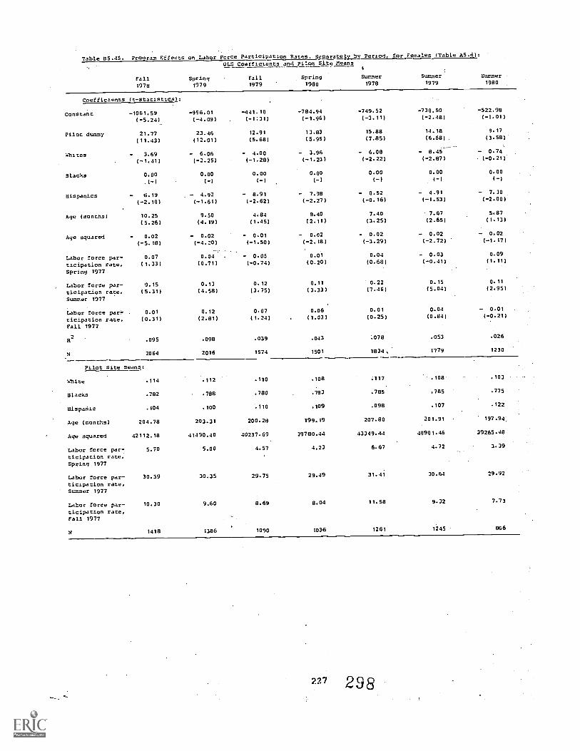
Table 85.45. Program Effects on tabor Force Participation Rates. secaratelyinv Period, for Females (Table A5.6):


Fall1978

Spring1979

Fall1979

Spring1980


Constant -1061.59 -956.01 -441.10 -784.94

( -5.24) ( -4.09) (-1.31) ( -1.96)

Pilot dummy 21.77 23.46 12.91 13.83

(11.43) (12.01) (5.68) (5.95)

Whites 3.69 - 6.06 - 4.00 - 3.96

( -1.41) ( -2.25) (-1.28) (-1.23)

Blacks 0.00 0.00 0.00 0.00

(-) (-) (-) (-)

Hispanics 6.19 - 4.92 - 8.91 - 7.98

(-2.10) (-1.61) (-2.62) ( -2.27)

Age (months) 10.25 9.50 4.84 9.40

(5.26) (4.19) (1.45) (2.11)

Age squared 0.02 - 0.02 - 0.01 - 0.02

( -5.18) (-4.20) (-1.50) (-2.18)_ _

.

Labor force par- 0.07 0.04 . - 0.05 0.01

ticipation rate, (1.33) (0.71) (-0.74) (0.20)

Spring 1977

Labor force par- 0.15 0.13 0.12 0.11

ticipation rate, (5.31) (4.58) (3.75) (3.33)

Summer 1077

Labor force par= 0.01 0.12 0.07 0.06

ticipation rate, (0.31) (2.81) (1.24) (1.03)

82

Fall 1977


.095 .098 .039 .043

.14 2064 2016 1574 1501

Pilot site means.

White .114 .112 .110 .108

Blacks .782 .788 .780 .783

Hispanic .104 .100 .110 .109

Age (months) 204.78 203.31 200.28 199.19

Age squared 42112.18 4(490.40 40237.69 39780.44

Labor force par -_ 5.00 4.57 4.23

ticipation rate,Spring 1977

Labor force par- 30.39 30.35 29.75 29.49

ticipation rate,Summer 1977

10.30 9.60 8.69 8.04

N 1418 1386 1090 1036

Summer1978

-749.52(-3.11)

15.88

(7.85)

- 6.08(-2.22)

0.00( -)

0.52.(-0.16)

7.40(3.25)

- 0.02

(-3.29)

0.04(0.68)

0.22(7.46)

0.01

(0.25)

.078

1834,

.117

.785

.098

207.80

43349.44

6.67

31.41

11.58

1261

227 2 5

Summer Summer1979 1980

-730.50 -522.98

(-2.48) (-1.01)

14.18 9.17

(6.68) (3.58)

,

- 0.74

(-2.87) (-0.21)

0.00 0.00

(-) (-)

- 4.91 - 7.30

(-1.53) (-2.00)

7.67 5.87

(2.65) (1.13)

- 0.02 - 0.02

(-2.72) (-1.17)

- 0.03 0.09

(-0.41) (1.11)

0.15 0.11

(5.04) (2.95)

0.04 - 0.01

(0.84) (-0.21)

.053 .026

1779 1230

.108' .103

.785 .775

.107 .122

201.91 197.94:

40901.46 39265.48

4.72 3.39

30.64 29.92

9.32 7.73

1245 866

ame 95.46. Pre:cram :Effects on Emmloyment Rates. Separately by Period. for 1hite Males (Table A5.71:

Suer1980

Fall1978

Spring1979


Surer1979

Fall1979

Spring1980

Surer1978


Constant -1174.81 -920.43 -1964.13 -311.25 -363.37 258.61 1925.28(-1.71) (-1.14) (-1.63) (-0.20) (-0.44) (0.25) (0.90)

-

Pilot dummy 17.69 16.27 5.31 14.29 11.17 - 3.12 9.14(2.99) (2.67) (0.78) (2.10) (1.71) (-0.47) (1.23)

Age (months) 11.33 8.96 19.06 2.81 4.09 - 2.03 - 19.11

(1.71) (1.15) (1.61) (0.18) (0.52) (-0.20) (-0.89)

Age squared - 0.03 - 0.02 0.05 0.01 - 0.01 0.00 0.05(-1.68) (-1-12) (-1.56) (-0.14) (-0.57) (0.21) (0.90)

Employment rates, - 0.01 0.07 0.04 - v.10 0.02 0.07 0.03Spring 1977 (-0.13) (0.88) (0.43) (-0.95) (0.24) (0.79) (0.25)

Employment rates, 0.03 0.07 0.07 0.26 0.05 0.06 0.12Summer 1977 (0.43) (0.95) (0.83) (3.01) (0.62) (0.71) (1.25)

Employment rates, 0.26 0.15 0.10 G.07 0.23 0.03 0.16

Fall 1977 (3.48) (1.95) (1.18) (0.87) (2.75) (0.37) (1.72)

R2 .116 .093 .075 .117 .073 .019 .087

239 232 194 178 217 206 149

Pilot site means:

Age (iontbs) 204.90 204.23 201.93 199.77 207.55 202.98 198.37

Age '',squared 42167.15 41882.69 40921.65 40016.17 43246.03 41363.23 39433.78

Emiloyment rates, 22.45 21.84 21.05 17.21 25.89 21.70 18.38

Spring 1977

Employment rates, 38.16 37.67 36.46 35.44 39.88 36.78 39.27

Summer 1977


Fall 1977

N 127 126 107 96 114 113 79

Table 85.47. Prooram Effects on Employment Rates. Separately by Period. for Black Males (Table A5.71:



1978 1979 1980 1978 1979 1980


Constant -1173.46 -1177.46 410.65 -165.58 -404.57 -789.91 - 419.98.

( -3.99) (-3.58) (0.94) (-0.32) (-1.19) (-1.93) (-0.62)

Pilot dummy 21.44 25.61 19.96 18.32 12.58 8.37 9.89(7.69) (9.09) (6.40) (5.70) (4.17) (2.77) (2.87)

Age (months) 11.11 11.18 - 3.91 2.07 4.02 8.20 4.78(3.92) (3.50) (-0.91) (0.40) (1.25) (2.05) (0.70)

Age squared - 0.03 - 0.03 0.01 - 0.01 0.01 - 0.02 - 0.01

(-3.77) (-3.34) (0.94) (-0.42) (-1.21) (-2.05) (-0.72)

Employment rates, - 0.03 0.00 - 0.04 - 0.01 - 0.00 - 0.06 0.07

Spring 1977 (-0.68) (0.10) (-0.74) (-0.14) (-0.08) (-1.26) (1.26)


Summer 1977 (2.16) (2.28) (1.69) (1.10) (5.40) (3.46) (1.12)

Employment rates, 0.08 0.01 0.04 0.01 - 0.01 - 0.01 - 0.02

Fall 1977 (2.06) (0.23) (0.98) (0.32) (-0.31) (-0.12) (-0.42)

R2 .080 .091 .043 .032 .049 .022 .014

N 1349 1331 1121 1067 1208 1226 903

Pilot site means:

Age (montba) 204.62 203.67 200.58 199.50 208.07 202.09 197.76

Age squared 42048.72 41645.89 40359.41 39909.77 43460.84 40982.67 39192.77

Employment rates, 11.52 11.31 9.78 9.51. 12.68 10.85 8.76

Spring 1777

Employment rates, 35.82 35.44' .... 31.11W, 31.14 37.04 33.90 32.70

Summer 1977


Pall 1977

N 975 967 807 768 858 887 653

228

299

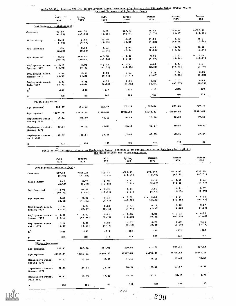
Table 95.48. Pro cram Effects on EmPloyment Rates. Separately by Period. for Hispanic Males (Table A5.71:


Fall1978

Spring1979

Fall Spring Summer

1979 1980 1978

Summer1979

Summer1980


Constant

Pilot dummy

Age (months)

Age squared

Employment rates.Spring 1977

Employment rates.Summer 1977

Employment rates.Fall 1977

R2

- 198.83

( -0.25)

- 51.50

(-0-06)

3.25 - 837.17

(0.00) (-0.50)

- 0.44 3.61 12.19 12.00

(-0.06)

1.91(0.25)

- 0.00

(0.49)

0.61(0.07)

- 0.00

(-0.19) (-0-02)

(1-39)

0.53(0.04)

25.43 1241.38(0.03) (1.16)

11.01 - 1.58

(1.35) (1.52)

8.94(0.54)

(-0.21)

0.06 - 11.74

(0.01) (-1.12)

-1525.76( -0.67)

15.07(1.64)

16.20(0.71)

- 0.00 - 0.02 0.00 0.03 0.04

(-0.04) (-0.55) (0.01) (1.14) (-0.73)

- 0.10 0.02 - 0.12 - 0.11 0.03 - 0.17

(-0.94) (0.20) (1.01) (-0.95) (0.31) (-1.70)

0.08 0.10 0.08 0.03

(0.93) (1.27) (0.85) (0.31)

0.23 0.14

(2.85) (1.78)

0.01(0.10)

0.05"

(0.58)

0.10 0.05 0.08 0.11 0.08 0.03 0.05

(1.18) (0.65) (0.85) (1.16) (1.04) (-0.37) (0.53)

.042 .048 .031 .033 .113 .035 .039

188 180 148 144 169 166 121

Pilot site means:

Age (months) 207.77 206.03 202.49 202.14 209.84 204.25 199.76

Age squared 43371.36 42623.95 41124.02 40976.60 44211.43 . 41859.94 39992.09

Employment rates. 23.74 22.57 19.43 18.01 25.28 20.89 19.60

Spring 1977


Summer 1977


Fall 1977

132 126 103 100 120 117 87

Table B5.49. Program Effects on Employment Rates. Separately by Period. for White Females 'Table A5.7)?


Fall1978.

Spring1979

Fall Spring Summer Summer Summer

1979 1980 1978 1979 1980


Constant

Pilot dummy

Age (months)

Age squared


317.92(0.51)

-1076.37(-1.52)

743.43 -520.95

(0.83) (-0.51)

5.00 0.70 - 3.49

(0.92) (0.13) (-0.55)

- 2.98(-0.50)

10.52

(1.54)

- 7.19

(-0.81)

271.717 -448.97

(-0.40) (-0.51)

5.43 0.10 - 0.48

(0.81) (0.02) (-0.013)

5.84 2.56 4.73

(0.57) (0.40) (0.55)

0.01 0.02 0.02 0.02

(0.53) (-1.52) (0.83) (-0.60)

0.14 0.26 0.02 0.13

(1.50) (2.61) (0.15) (0.94)

Employment rates. - 0.14 0.07

Summer 1977 (-1.68) (-0.88)

Employment rates. 0.22

Pall 1977

0.23(2.49) (2.57)

0.01 - 0.08

(0.13) (-0.70)

0.08 0.27

(0.75) (2.12)

- 0.01 - 0.01

(-0.36) (-0.55)

0.18 0.22(1.96) (2.02)

0.02 - 0.02

(0.25) (-0.25)

0.21 0.09

(2.30) (0.90)

-739.25(-0.51)

3.93(0.52)

8.57(0.59)

0.02

(-0.63)

0.27(1.81)

- 0.20(-1.46)

0.26(1.75)

2 .056 .092 .014 .052 .102 .033 .067

286 274 213 201 263 233 160

Pilot site means:

Age (months)

Age squared



207.13

43108.31

14.52

22.33


Fall.1977

205.86

42558.03

13.24

201.98

40940.10

12.38

21.41 22.09

18.89 17.33

200.52

40327.84

11.48

210.00

44294.19

16.26

20.54 23.20

15.39 21.81

203.91

41728.63

12.48

197.64

39141.24

10.61

22.53 18.37

18.17 13.75

162 155 120 112 148 134 89

229

3 0

Table 35.50. Procram Effects on Employment Rates. SeParately by Period. for Slack Females (Table A5.71:OLS Coefficients and Pilot Site Means

Fall1978


Constant

Pilot dummy

-1615.92(-6.22)

29.98

Age (months)

(12.17)

15.50

(6.20)

Age squared - 0.04(-6.13)

Employment rates, - 0.14Spring 1977 (-2.34)

Employment rates, 0.12Summer 1977 (3.90)


Fall 1977

32

N

(0.91)

.118

1568

Spring Fall Spring1979 1979 1980

-1263.75 -634.60 -311.00(-4.27) ( -1.49) (-0.61)

32.16 23.64 21.30

(12.72) (8-18) (7.13)

12.41 6-91 3.84(4.31) (1.64) (0.76)

- 0.03 - 0.02 - 0.01

(-4.31) ( -1.76) (-0.87)

- 0.08 - 0.03 0.01

(-1.38) ( -0.37) (0.11)

0.12 0.03 0.02

(3.80) (0.93) (0.42)

0.05 0.09 0.13(1.34) (1.87) (2.60)

Pilot site means:

Age (months) 204.48



Spring 1977

Employment rates. 20.90Summer 1977

Employment rates, 11.12Fall 1977

1109

.113

1542

.070

1192

.062

1140

203.08 200.01 199.01

41392.54 40125.23 39708.04

3.49 3.16 3.C2

21.49 19.30 19.28

10.83 9.72 9.34

1092 850 811

Summer Summer Summer1978 1979 1980

-1231.41(-3.85)

20.83(7.68)

12.11(4.00)

- 0.03(-4.08)

- 0.16(2.67)

7-13.25'-'"--r-(7.70)

-952.12 -212.29( -2.42) (-0.31)

14.31 10.47(4.97) (3.05)

9.99 2.95(2.58) (0.43)

- 0.03( -2.66)

- 0.11

( -1.49)

- 0.01(-0.50)

- 0.07(-0.79)

0.11 0.06

(3.16) (1.46)

0,!,A 0.01 0.04

f1.73) (0.28) (0.68)

.100 .035 .023

1396 1362 925

207.46

43200.34

4.22

21.56

11.96

989

201.67

40803.36

3.41

197.90

39248.67

2.61

21.81 20.53

10.67 9.61

978 671

Table 85.51. Proaram Effects on Employment Rates. Separately by Period, for Hispanic Females (Table A5.7):OLS Coefficients and Pilot Site Means

Fall Spring Fall Spring

1978


Constant

Pilot dummy

Age (months)

Age squared


-914.45(-1.38)

15.91

(2.34)

8.69

(1.37)

- 0.02(-1.32)

0.14

(1.26)

Employment rates. 0.18Summer 1977 (2.41)

Employment rates, 0.04

Pall 1977 (0.46)

R2 .126

N 210

Pilot site means:

Age (months)

Age squared



Employment rates.Fall 1977

N

204.41

41976.11

12.17

40.93

26.65

147

1979 1979 1980

-1361.90 25.18 -1467.76( -1.50) (0.02) (-0.80)

11.22 - 7.64 - 10.29(1.53) (-0.98) (-1.24)

14.06 0.30 15.14(1.58) (0.02) (0.83)

- 0.04 - 0.00 - 0.04(-1.64) (-0.04) (-0.83)

0.19 0.11 0.11

(1.57) (0.79) (0.78)

0.15 0.25 0.21

(1.90) (2.88) (2.28)

0.02 0.02 - 0.03

(0.27) (0.16) (-0.31)

.098

200

.084

169

.064

160

102.30 200.53 199.16

41068.72 40331.85 39757.55

11.43 10.74 9.29

41.85 40.30 40.58

26.02 22.38 22.88

139 120 113


-920.84 -1368.78 -842.52(-1.02) (-1.18) (-0.41)

31.50 9.17 20.04(4.05) (1.14) (2.34)

9.11 14.43 8.95

(1.07) (1.26) (0.43)

- 0.02 - 0.04 - 0.02(-1.10) (-1.31) (-0.45)

- 0.03 - 0.03 0.16

(-0.28) (-0.24) (1.05)

0.19 0.10 0.28

(2.15) (1.20) (3.13)

0.09 0.05 - 0.01

40.95) (0.57) (-0.06)

.158

175

.054

184

.163

145

207.94 201.64 198.47

43411.09 40789.38 39476.25

14.43 11.20 8.44

43.68 42.98 40.91

28.37 25.69 22.74

124 133 106

230 301

Table B5.52. Program Effects on Employment Rates, S9arately by Period, for Whites (Table A5.7):


Fall

1978

Spring

1979

Fall

1979

Spring

1980

Summer

1978

Summer

19/9

Summer

1980


Constant' -298.78 -924.23 -143.77 -323.27 -101.55 -102.34 553.92

(-0.65) (-1.75) (-0.20) (-0.38) (-0.19) (-0.15) (0.48)

Pilot dummy 11.05 8.19 - 0.07 9.60 5.55 - 1.38 7.70

(2.76) (2.01) (-0.01) (2.01) (1.31) (-0.31) (1.46)

Male 9.03 10.77 13.49 11.47 11.21 18.44 10.52

(2.22) (2.60) (2.86) (2.35) (2.59) (4.06) (1.94)

Female

Age (months)

0.00

(-)

2.89

0.00

(-)

8.98

0.00

(-)

1.36

0.00

(-)

3.44

0.00

(-)

1.17

0.00

(-)

1.33

0.00

(-)

- 4.94

(0.65) (1.76) (0.19) (0.41) (0.24) (0.21) (-0.42)

Age squared - 0.01 - 0.02 - 0.00 - 0.01 - 0.00 - 0.00 0.01

(-0.61) (-1.72) ( -0.14) (-0.40) (-0.24) (-0.21) (0.40)

Employment rate, 0.07 0.15 0.05 0.03 0.09 0.13 0.15

Spring 1977 (1.05) (2.36) (0.66) (0.32) (1.36) (1.92) (1.70)

Employment rate, - 0.05 0.01 0.05 0.11 0.04 0.02 - 0.00

Summer 1977 (-0.94) (0.17) (0.71) (1.71) (0.66) (0.34) (-0.06)

Employment rate, 0.23 0.18 0.09 0.14 0.21 0.06 0.17

Fall 1977 (4.07) (3.07) (1.30) (1.91) (3.56) (0.90) (2.17)

R2

.082

N 525

.102

506

.058

407

.078

379

Pilot site means;

Male .4:, .448 .471 .462

Female .561 .552 .529 .538

Age (months) 206.15 205.13 201.96 200.17

Age squared 42694.72 42255.21 40931.41 40183.99

Employment rate, 18.00 17.09 16.46 14.12

Spring 1977

Employment rate, 29.29 28.70 28.87 27.42

Summer 1977

Employment rate, 23.64 22.89 23.40 20.72

Fall 1977

289 281 227 208

.096 .071 .073

480 439 309

.435 .457 .470

.565 .543 .530

208.94 203.49 197.98

43838.12 41561.46 39278.80

20.45 16.70 14.26

30.46 29.05 28.20

26.07 23.64 21.61

262 247 168

Table B5.53. Program Effects on Employment Rates, Separately by Period, for Blacks (Table A5.7):

Summer1980

Fall

1978

Spring1979


Summer1979

Fall1979

Spring1980

Summer1978


Constant -1431.39 -1222.68 -79.39 -214.38 -820.35 -855.71 *14.87(-7.33) (-5.54) (-0.26) (-0.59) (-3.52) (-3.02) (-1.65)

Pilot dummy 26.10 29.20 21.80 19.77 16.79 11.49 10.10(14.12) (15.50) (10.26) (9.03) (8.31) (5.52) (4.16)

Male 3.11 3.38 7.40 8.05 5.10 8.63 10.55(1.84) (1.96) (3.83) (4.04) (2.74) (4.56) (4.82)

Female 0.00 0.00 0.00 0.00 0.00 0.00 0.00(-) (-) (-) (-) (-) (-) f-)

,Age (months) 13.65 11.81 1.14 2.68 8.07 8.90 3.81(7.27) (5.51) (0.38) (0.75) (3.65) (3.20) (0.79)

Age squared 0.03 0.03 - 0.00 - 0.01 - 0.02 - 0.02 - 0.01(-7.11) (-5.40) (-0.44) (-0.83) (-3.69) (-3.26) (-0.85)

Employment rate, 0.06 0.03 - 0.04 - 0.01 - 0.06 - 0.07 0.03Spring 1977 (1.85) (-0.80) (-0.92) (-0.18) (-1.72) (-1.83) (0.59)

Employment rate, 0.09 0.09 0.05 0.03 0.22 0.11 0.05Summer 1977 (4.19) (4.30) (1.93) (1.11) (9.12) (4.65) (1.82)

Employment rate, 0.06 0.03 0.07 0.07 0.02 0.00 0.01Fall 1977 (2.21) (1.09) (2.02) (1.95) (0.54) (0.15) (0.16)

R2

.098 .100 .057 .052 .074 .035 .030

N 2917 2873 2313 2207 2604 2588 1828

Pilot site means:

Male .468 .470 .487 .486 .465 .476 .493

Female .532 .530 .513 .514 .535 .524 .507

Age (months) 204.55 203.36 200.28 199.25 207.74 201.87 197.83

Age squared 42014.65 41511.53 40239.29 39806.16 43321.35 40888.64 39221.10

Employment rate, 7.36 7.16 6.38 6.18 8.15 6.95 5.64Spring 1977

Employment rate, 27.88 28.04 25.39 25.05 28.75 27.56 26.53Summer 1977

Employment rate, 16.04Fall 1977

15.51 13.83 13.30 17.840 I)la;

15.15 13.44

2084 2059 1657 1579 1847 1865 1324

Table 85.54. Program Effects on Employment Rates, Separately by Period, for Hispanics (Table A5.7):

Fall1978

Spring1979


Summer Summer

1979 1980Fall1979

Spring1980

Summer1978


Constant -732.10 -649.01 -33.83 -942.23 -384.07 -47.09 -1724.41(-1.46) (-1.05) (-0.03) (-0.78) (-0.63) (-0.06) (-1.15)

Pilot dummy 8.49 9.05 1.98 0.57 21.71 4.74 18.17(1.66) (1.75) (0.34) (0.10) (4.12) (0.85) (2.94)

Male 12.36 15.60 21.27 17.94 16.18 15.64 18.27(2.61) (3.24) (3.99) (3.27) (3.33) (3.10) (3.28)

Female 0.00 0.00 0.00 0.00 0.00 0.00 0.00(-) (-) (-) (-) (-) (-) (-)

Age (months) 6.95 6.69 0.75 9.78 3.93 1.69 17.88(1.44) (1.11) (0.08) (0.81) (0.68) (0.14) (1.20)

Age squared - 0.02 - 0.02 - 0.00 - 0.02 - 0.01 - 0,00 0.05(-1.38) (-1.12) (-0.09) (-0.82) (-0.69) (-0.17) (-1.22)

Employment rate, 0.00 0.10 - 0.02 - 0.01 0.01 - 0.11 0.07Spring 1977 (0.04) (1.25) (-0.17) (-0.10) (0.08) (-1.39) (0.70)

Employment rate, 0.15 0.14 0.16 0.12 0.22 0.13 0.18Summer 1977 (2.55) (2.42) (2.61) (1.79) (3.74) (2.22) (2.78)

Employment rate, 0.08 0.05 0.06 0.U5 0.09 0.02 0.02Fall 1977 (1.29) (0.81) (0.83) (0.76) (1.51) (0.26) (0.26)

R2 .092 .090 .093 .064 .163 .051 .137

N 398 380 317 304 344 350 266

Pilot site means:

Male .473. .475 .462 .469 .492 .468 .451

Female .527 .525 .538 .531 .508 .532 .549

Age (months) 206.00 204.08 201.43 200.56 208.88 202.86 199.05

Age squared 42636.23 41808.19 40697.74 40329.87 43804.70 41290.40 39708.77

Employment rate, 17.64 16.73 i+.76 13.39 19.77 15.73 13.47Spring 1977

Employment rate, 45.03 45.32 43.76 43.34 47.81 45.76 43.43Summer 1977

Employment rate, 33.40 32.01 29.39 29.83 35.73 31.48 29.28Fall 1977

N 279 265 223 213 244 250 193

Table B5.55. Program Effects on EmployFent Rates, Separately by Period, for Males (Table A5.7):OLS Coefficients and Pilot Site Means

Fall

1978

Spring1979

Fall

1979

Spring1980

Summer1978

Summer197 3

Siam.r198(


Constant -1085.00 -1049.31 139.33 -192.95 -377.08 -489.40 -278.25

(-4.26) (-3.66) (0.36) (-0.41) (-1.28) (-1.38) (-0.45)

Pilot dummy 18.19 21.59 16.45 16.75 11.89 5.58 10.28

(7.59) (8.95) (6.11) (6.09) (4.65). (2.16) (1.49)

White 6.16 9.86 7.12 8.33 0.32 1.89 5.72

(1.87) (2.97) (1.91) (2.16) (0.09) (0.53) (1.39)

Black 0.00 0.00 0.00 0.00 0.00 0.00 0.00

(-) (-) (-) (-) (-) (-) ( -)

Hispanic 10.00 18.07 15.70 12.41 17.59 8.38 10.57(2.77) (4.94) (3.79) (2.97) (4.53) (2.15) (2.37)

Age (months) 10.30 9.98 - 1.26 2.26 3.82 5.24 3.33(4.20) (3.59) (-0.32) (0.49) (1.37) -(1.50) (0.54)

Age squared - 0.02 0.02 0.00 - 0.01 - 0.01 - 0.01 - 0.01

(-4.05) (-3.43) (0.36) (-0.49) (-1.35) (-1.50) (-0.56)

Employment rate, - 0.03 0.02 - 0.03 - 0.03 0.00 - 0.05 0.06

Spring 1977 (-0.93) (0.58) (-0.66) (-0.58) (0.13) (-1.24) (1.38)

Employment rate, 0.06 0.07 0.06 0.06 0.17 0.12 0.05

Summer 1977 (2.26) (2.66) (1.94) (1.97) (5.65) (3.90) (1.42)

Employment rate, . 0.11 0.04 0.06 0.04 0.04 - 0.00 0.02

Fall 1977 (3.61) (1.24) (1.73) (1.13) (1.23) (-0.08) (0.54)

R2

.079 .095 .047 .040 .068 .020 .024

N 1776 1743 1463 1389 1594 1598 1173

Pilot site means:

White .103 .103 .105 .100 .104 .101 .096

Black .790 .794 .794 .796 .786 .794 .798

Hispanic .107 .103 .101 .104 .110 .105 .106

Age (months) 204.99 203.97 200.91 199.80 208.21 202.41 198.03

Age squared 42202.39 41:1At.47 40496.01 40031.04 43520.90 41113.06 39300.92

Employment rate, 13.95 13.56 11.94 11.16 15.45 13.00 10.84

Spring 1977

Employment rate, 37.53 37.09 33.92 33.16 38.99 35.76 34.80

Summer 1977

Employment rate, 24.40 23.36 21.39 20.52 7 ..... 27.41 23.00 20.74

Fall 1977 L.: ii a1

N 1234 1219 1017 964 1092 1117 819

Table 85.56. Program Effects on Employment Rates, Separately by Period, fox Females

OLS Coefficients and pilot Site Means

(Table A5.7):

Summer1979

Summer1980

Fall1978

Spring1979

Fall1979

Spring1980

Summer1978


Constant -1287.58 -1191.01 -332.12 -402.52 -967.04 -828.11 -372.10

(-5.69) (-4.54) (-0.90) (-0.91) (-3.51) (-2.42) (-0.63)

Pilot dummy 24.93 25.61 16.60 15.86 18.66 11.73 11.36

(11.64) (11.60) (6.63) (6.13) (7.99) (4.74) (3.88)

White 0.56- 0.74 - 0.06 1.17 - 5.62 -. 8.85 3.90

(0.19) (0.24) (-0.02) (0.33) (-1.79) (=2.59) (0.97)

Black 0.00 0.00 0.00 0.00 0.00 0.00 r.00

(-) ( -) (-) ( -) ( -) (-) %)

Hispanic 0.22 4.44 0.30 0.64 4.29 1.44 i.91

(0.07) (1.28) (0.08) (0.16) (1.15) (3.36) ( '.22)

Age (months) 12.34 11.76 3.84 4.71 9.51 8.77 4.54

(5.67) (4.62) (1.05) (1.07) (3.65) (2.61) (0.77)

Age squared - 0.03 - 0.03 - 0.01 - 0.01 - 0.02 - 0.02 - 0.01

(-5.58) (-4.62) (-1.14) (-1.17) (-3.71) (-2.70) -0.85)

Employment rate, - 0.02 0.04 0.01 0.07 - 0.06 - 0.01 0.07

Spring 1977 (-0.34) (0.85) (0.26) (1.12) (-1.25) (-0.27) (0.97)

Employment rate, 0.09 0.09 0.05 0.03 0.23 0.09 0.07

Summer 1977 (3.44) (3.40) (1.66) (0.77) (7.75) (2.95) (2.10)

Employment rate, 0.06 0.08 0.08 0.12 0.08 0.03 0.05

Fall 1977 (1.76) (2.32) (1.89) (2.90) (2.18) (0.86) (1.05)

R2

.088 .086 .040 .044 .093 .034 .031

1 N 2064 2016 1574 1501 18341,

1779 1230

Pilot site means:

White .114 .112 .110 .108 .117i

.108 .103

Black .782 .788 .780 .783 .785 I

.

.785 .775

,Hispanic .104 .100 .110 .109 .098 .107 .122

Age (months) 204.78 203.31 200.28 199.19 207.80 201.91 19/.94

Age squared 42112.18 41490.40 40237.69 39780.44 43349.44. 40901.46 39265.48

Employment rate, 5.82 5.38 5:01 4.62 6.63 5.22 4.15

Spring 1977

Employment rate, 23.14 23.52 21.92 21.74 23.93 24.15 22.81

Summer 1977

Employment rate, 13.73 13.26 11.95 11.47 14.73 13.08 11.64

Fall 1977

N 1418 1386 1090 1036Q 1261 1245 866

auv

Cable 85.57. Program Effects on Labor Force Participation Rates. Separately by Period,for the 15-16 Year Old Cohort Excluding Denver/Phoenix (Table A5.911


Fall Spring Fall Spring1978 1979 1979 1980


Coefficients (t-statistics13

Constant -2133.43 - 1278.57 -1354.96 -1276.15 -4847.74 - 880.43 -1046.31(-1.42) 1-0.97) ( -1.53) (-1.44) 1-1.641 (-0.74) ( -1.17)

Pilot dummy 24.57 25.95 19.66 20.39 17.46 15.44 11.49(11.85) (12.27) (8.94) (9.14) (7.33) (7.21) (4.95)

White male 6.41 7.09 0.87 0.75 5.12 6.67 0.10(1.49) (1.61) (0.19) (0.16) (1.03) (1.49) (0.02)

Black =ale 0.00 0.00 0.00 0.00 0.00 0.00 0.00( -) (-) (-) (-) (-) ( -) (-)

Hispanic male 8.22 - 3.72 5.52 - 16.34 - 3.07 - 3.56 - 21.99(0.36) (-0.16) (0.23) (-0.69) (-0.13) (-0.15) (-0.96)

White female - 5.61 - 8.77 - 12.18 - 10.48 - 13.28 - 21.97 - 7.94(-1.41) ( -2.15) (-2.84) (-2.44) (-2.86) ( -5.21) (-1.80)

Black female 0.33 1.16 - 4.93 - 5.90 - 1.07 - 3.22 - 9.08(0.16) (0.55) (-2.22) (-2.61) (-0.44) ( -1.51) (-3.96)

Hispanic female 4.05 4.97 - 9.13 11.94 28.15 5.70 16.01(0.32) (0.39) (-0.66) (-0.87) (1.58) (0.45) (-1.13)

Age (months) 20.76 12.41 14.18 13.44 48.69 9.04 11.15(1.34) (0.92) (1.54) (1.46) (1.62) (0.74) (1.20)

Age squared - 0.05 - 0.03 0.04 - 0.03 - 0.12 0.02 0.03

Labor force par-ticipation rate,Spring 1977



R2

N

(-1.25)

0.02

(-0.85) (-1.51)

0.01 - 0.08(0.28) (0.12)

(-1.43) (-1.59)

- 0.02 - 0.00(-1.05) (-0.27).

0.14 0.12 0.09(4.52) (4.07) (2.82)

0.03 0.01 0.09(-0.51) (0.14) (1.54)

(-0.70) (-1.18)

- 0.09 - 0.05(-0.00) (-1.26)

0.06 0.19(1.95) (5.47)

0.07 - 0.03(1.10) (-0.51)

(-0.69)

0.16 0.06(5.02) (1.70)

0.02 0.06(0.40) (0.98)

.115 .107 .064 .063 .081 .070 .036

1668 1714 1603 1600 1264 1652 1401

Pilot site means:'

White male .045 .044 .045 .045 .044 .043 .044

Slack male .407 .407 .424 .424 .398 .418 .437.

Hispanic =ale .002 .002 .002 .002 .002 .002 , .002

White female .055 .053 .054 .054 .055 .051 .057

Black female .485 .488 .470 .469 .497 .480 .455

Hispanic female .006 .006 .005 .006 .004 .006 .005

Age (months) 194.12 193.80 193.01 193.00 196.41 193.47 192.96

Age squared 37709.28 37590.40 37284.51 37281.71 38595.19 37461.87 37269.44...--.

Labor force par-, 3.17 3.07 3.28 3.29 3.70 3.17 3.26tieipation rate, _ ...... _

Spring 1977

Labor force par- 29.91 29.69 29.38 29.43 31.17 30.05 30.26ticipation rate,Summer 1977

Labor force par- 6.17 6.00 5.84 5.85 7.32 6.12 6.02tiCipation rate,Fall 1977

1136 1171 1093 1091 841 1129 970

236.

Table 85.58. Prooram Effects on Employment Pates. Secaratelv by Period.for the 15-15 Year Old Cohort excluding Denver/Phoenix (Table A5.91;

OLS Coefficients and pilot Site means

Fall1978

Spring1979

Fall.1979

Spring1980

Sumter1978

Summer19 79

Summer1980

Coefficients (t-statistics13

Constant -3962.71 -816.47 -21e6.ao -2782.63 -6748.14 -1721.67 -1743.91

(-2.36) (-0.56) (-2.19) (-2.79) (-1.95) (-1.23) (-1.67)

Pilot dummy 25.98 28.76 24.06 25.54 14.81 9.57 13.24

(11.25) (12.19) (9.611 (10.19) (5.27) (3.77) (4.86)

White =ale 5.55 7.93 1.41 1.48 1.14 3.28 1.26

(1.17) (1.63) (0.28) (0.29) (0.20) (0.62) (-0.23)

Black male 0.00 0.00 0.00 0.00 0.00 0.00 0.00

( -) (-) (-) ( -) (-) (- ( -)

Hispanic male 31.51 9.97 - 10.46 - 47.24 - 9.11 - 26.40 - 38.93

(1.26) (-0.3B) (-0.39) (-1.77) (-0.34) (-0.96) (-1.45)

White female 3.70 - 3.38 - 9.40 - 2.93 - 18.17 7 26.47 - 3.88

(-0.84) (-0.75) (-1.95) (-0.61) (-3.34) (-5.31) (-0.75)

Black female - 1.14 1.34 - 4.83 - 6.08 - 2.42 - 6.56 - 9.43

(-0.49) (0.57) (-1.94) (-2.44) . (-0.85) (-2.60) (-3.52)

Hispanic female 0.31 2.71 1.38 - 19.34 40.83 4.94 - 11.87

(0.02) (0.19) (0.09) (-1.25) (1.96) (0.33) (-0.72)

Age (months) 39.31 7.44 22.99 29.44 68.04 17.95 1E1.80

(2.28) (0.49) (2.22) (2.84) (1.93) (1.24) (1.73)

Age squared - 0.10 - 0.02 - 0.06 - 0.08 - 0.17 - 0.05 - 0.05

(-2.18) (-0.42) (-2.22) (-2.87) (-1.90) (-1.22) (-1.75)

Employment rate, - 0.06 0.02 - 0.02 0.05 - 0.11 - 0.01 0.05

Spring 1977 (-1.12) (0.42) (-0.32) (0.92) (-1.86) ( -0.20) (0.77)

Employment rate, 0.11 0.09 0.04 0.03 0.22 0.13 0.05

Summer 1977 (3.82) (3.10) (1.11) (1.03) (6.32) (3.96) (1.38)

Employment rate, - 0.01 - 0.01 0.05 0.05 0.00 - 0.06 0.02

Fall 1977 (-0.27) (-0.20) (1.30) (1.16) (0.00) (-1.33) (0.41)

R2 .110 .100 .066 .076 .076 .041 .033

N 1668 1714 1603 1600 1264 1652 1401

Pilot site means;

White male .045 .044 .045 .045 .044 .043 .044

Black male .407 .407 .424 .424 .398 .418 .437

Hispdni.0 male .002 .002 .002 .002 .002 .002 .002

White female .055 .053 .054 .054 .055 .051 .057

Black female .485 .488 .470 .469 .497 .480 .455

Hispanic female .006 .006 .005. .006 .004 .006 .005

Age (months) 194.12 193.80 193.01 193.00 196.41 193.47 192.96

Age squared 37709.28 37590.40 37284.51 37281.71 38595.19 37461.87 37269.44

Employment rate, 4.11 4.02 4.02 4.43 4.15 4.01

Spring 1977

Employment rate, 22.14 22.04 21.17 21.21 23.09 22.33 22.21

Summer 1977

Employment rate, 10.69 10.37 10.39 10.40 12.55 10.67 10.77

Fall 1977

N 1136 1171 1093 1091 B41 1129 970

Table 88.1. Program Effects on the Percentage of Program-Eligible TimeSpent in Different School and Employment States (Table 6.1):


Coefficients (t-statistica):1 Pilot site means:

Variable

Percentage. of

time enrolled,employed

Percentage oftime enrolled,not employed

Percentage enot enrolledemployed

time

Constant - .503 - .034 .248 1.000(3.796) (.212) (2.083)

Pilot site .132 - .091 .020 1.000(17.116) (10.904) (3.212)

Age in June 1978 .699 .722 - .264 2.050(months/100) (5.309) (4.612) (2.237)

Age squared - .184 - .216 .097 4.230 .

(5.437) (5.460) (3.234)

White male - .027 - .003 .068 .048(2.443) (.371) (6.449)

Black male 0.000 0.000 0.000 .368(-) () (-)

Hispanic male - .010 - .059 .104 .049(.566) (3.073) (7.261)

White female - .037 - .038 - .007 .061

(2.556) (2.427) (.586)

Black female .021 .027 - .059 .420(2.535) (3.102) (8.917)

Hispanic female - .021 - .026 - .025 .054(1.300) (1.492) (1.853)

Proportion of pre-program time:

Enrolled, employed .229 - .263 .034 .057(9.114) (9.615) (1.682)

Not enrolled,employed

- .135(5.233)

- .425(15.173)

.401

(19.159).081

Not enrolled,not employed

- .215(2.925)

- .403(5.503)

.038(.512)

.282

R2

.169 .239 .207

4033 4033 4033 2778

1

Fitted values for the percentage of time not enrolled and not employed aie calculated by subtractingthe fitted values for the'three estimated categories from 100.

Table 86.2. Program Effects on the Percentage of Program-Eli:able Time Spent in Different

School and Emoloyeent States, by Pri=ary State in the Pre-croaram Period (Table 6.21:


Coefficients (t-statistics) :1Pilot site means:

Youths pri=arily enrolled.employed in oreoroaram'eeriod

Youths primarily enrolled, notemoloved in orenroaram period

Youths primarilyenrolled, em-ployed in pre-program period

Percentage of Percentage of

time enrolled, time enrolled,

Variable employed not employed

Percentage oftime not en-rolled, employed

Percentage oftime enrolled,employed

"Percentage oftime enrolled,not employed


Constant 1.434 1.602 3.832 -2.420 2.948 -1.257 1.000

(.357) (.468) (1.187) (2.511) (2.765) (2.035)

Pilot site .107 - .030 - .015 .166 - .131 .023 1.000

(2.404) (.788) (.416) (17.5621 (12.539) (3.829)

Age in -1.052 - .709 -3.996 2.599 -2.069 1.187 2.050

Jute 1978 (.271)

(months /100)

(.215) (1.283) (2.773) (1.995) (1.977)

Age squared .218 .082 1.043 - .653 .444 - .253 4.230

(.235) (.104) (1.397) (2.867) (1.763) (1.7341

White male .009 - .168 .094 - .033 - .090 .077 .119

1., (.158)

Black =ale 0.000

(3.390)

0.000

(1.998)

0.000

(1.537)

0.000

(3.792)

0.000

(5.618)

0.000 .488

(-) (-1 1-) (-) 1-) 1-)

Hispanic =ale .038 - .152 .120 - .023 - .079 .110 .104

(.553) (2.623) (2.1791 (.9881 (3.116) (7.475)

White female - .032 - .017 .032 - .035 - .048 - .002 .044

(.309) (194) (.384) (1.813) (2.238) (.192)

Black female .025 - .034 - .051 .026 .016 - .044 .193

(.436) (.720) (1.128) (2.743) (1.5281 (7.061)

Hispanic .250 - .092 - .033 - .041 - .052 .021 .052

female (2.9011 (1.257) (.479) (1.919) (2.186) (1.517)

Proportion ofpre-program time:

Enrolled, .116 - .231 .153 .409 - .555 .228 .637

employed (.752) (2.006) (1.308) (7.106) (8.725) (6.192)

Not enrolled,- .106 - .190 .294 - .051 - .510 .194 .169

employed (.368) (1.132) (1.439) (.660) (6.025) (3.963)

Not enrolled,- .230 .159 .043 - .381 - .401 .046 .058

not employed (1.80) (.277) (.043) (1.369) (1.452) (.1681

R2 .031 .115 .098 .135 .106 1.06

N 194 194 194 2995 2995 2995 135

Youths primarilyenrolled, notemployed in pre-program period

1.000

1.000

2.010

4.060

.036

.384

.040

.048

.444

.048

.028

.054

.189

2080

Variable

Coefficients 1t-stattstics1t1Pilot site means:

Youths primarily not enrolled,employed in orenrooram period

Youths primarily not enrolled, notemployed in orenrooram period

Youths primarilyenrolled, em-ployed in pre-program period

Youths primarilyenrolled, notemployed in pre-program period







Constant 1.453 -4.493 8.299 -1.899 1.563 -4.785 1.000 1.000

(.580) (1.614) (1.126) (1.633) (1.231) (2.645)

Pilot site .004 .005 - .037 .037 - .005 .033 1.000 1.000

(2.33) (.212) (.653) (3.001) (.359) (1.707)

Age in -1.189 4.347 -8.076 1.911 -1.085 4.630 2.230 2.190

June 1978(months/100)

(.521) (1.716) (1.204) (1.766) (.918) (2.749)

Age squared .276 -1.011 2.012 - .435 .244 -1.074 5.000 4.810

(.534) (1.762) (1.324) (1.739) (.893) (2.756)

White male - .061 - 0.021 .207 - .044 .046 .200 .053

(2.386) (.732) (2.759) (3.021) (1.613) (1.173)

239 31


Black male 0.000 ;

(-)

Hispanic - .071

male (2.353)

White - .038

female (1.298)

Black - .029

female (.970)

Hispanic .016

female (.356)

Proportion of

pre-program time:

Enrolled, .061

employed (.555)

Hot enrolled,- .118

employed' (1.447)

Not enrolled,- .164

not employed (1.88)

.064R2

0 H 147

0.000

(6)

0.000

(-)

0.000

(-)

0.000

(-)

0.000

(-1

.311 .272

.001 .051' - .026 .024 .063 .156 .047(.035) (.580) (.949) (.774) (1.451)

- .020 .076 - .073 . .038 - .069 '.133 .112(.618) (.877) (3.853) (1.818) (2.339)

- .010 - .096 - .025 .022 .122 .133 .438,(.306) (1.105) (1.718) (1.350) (5.327)

.005 - .079 - .066 - .014 - .101 .067 .078(.105) (.592) (2.891) (.564) (2.842)

.170 .011 .561 - .216 - .200 .069 .013(1.731) (.0371 (4.830) (1.708) (1.111)

- .124 .248 - .136 - .375 .561 .750 .049(1.819) (1.177) (2.236) (5.659) (5.931)

- .067 - .319 - .145 - .311 .015 .114 .791(.119)

(.4431 (.603) (1.300) (.061)

.068 .184 .126 .130 1.50

147 147 697 697 697 90 473


T

APPENDIX C

Tests of Sample Attrition Bias

241 313

APPENDIX C

In measuring program impacts for this report, we have restricted

attention to sample members.who responded to all three during-program

interviews:' Waves I, II, and III: Both Waves II and III are required if

our data'are to cover the period of full program operation. However, since

a significant portion of the original sample did not complete all the

interviews, this opens the possibility of bias in our results. Such-attri-

tion bias may occur if pilot site sample respondents are systematically

different from comparison site sample respondents in ways that are not

corrected for in our statistical analyses of the data.

In an attempt to test for the existence and magnitude of such bias,

a special survey of a subset of Wave II nonrespondents was undertaken

during Wave III data collection. That is, special efforts were made to

locate Hispanics in Denver and Phoenix and blacks in Baltimore and Cleveland

who had not responded to Wave II; those located were administered both

Waves II and III.1

The resulting attrition sample was then used to

estimate program efforts for survey nonrespondents; these results were then

compared with estimated efforts for otherwise identical respondents. The

result is a straightforward calculation of potential attrition bias,

utilizing a methodology which is likely to be more reliable than the

econometric techniques employed to estimate bias in our previous report.

(See Farkas et al. (1980: Appendix A1).)2

.Program Participation

Table C2.1 shows program participation rate estimates for the local

field survey and attrition survey samples, and estimated program participa-

tion rates in the absence of attrition for (a) Hispanic youths in Denver,

1Attention was restricted to particulcr race and site groups in an attemptto use limited resources to provide as much information as possibleconcerning the most substantively important program effects.

2The difficulty with econometric tests for attrition bias is that theyrely upon (necessarily) untested assumptions regarding relationships amongthe variables in the analysis. It should be noted, however, that ourprevious work in this regard concluded that sample attrition was not aproblem for'the analysis.

242

314

Hispanic youths in Denver:

Local field survey sample2

Attrition sample3

Estimated participation

re..tes in he absence of

Otrition

Bin); youths in Baltimore:

Local field survey sample

tN.1Attrition sample

A

315

Estimated participation

rates in the absence of

attrition

Table C2.1. Sam le Attrition Program Participation Rates'

Spring

1980

Summer

1980

Cumulative:

Spring 1978

through

Summer 1980

Spring

1978

Summer

1978

Fall

1978

Spring

1979

Summer

1979

Fall

1979

36.9 25.4 23.2 26.0 26.7 17.5 15.9 13.7

(268)

5(210) (232) (263) (2g50) (236) (211) (201) (183)

18.7 7.7 9.5 9.7 10.0 12.3 10.4 8.5 4.3

(150) (130) (137) (144) (140) (130) (115) (106) (92)

27.8 13.4 17.5 16.5 18.0 19.5 14.0 12.2 9.0

70.5 43.3 47.3 47.4 51.9 51.5 43.2 44.5 39.6

(999) (770) (842) (944) (933) (876) (745) (712) (624)

61.7 33.7 34.0 34.3 41.4 32.2 27.9 31.6 28.8

(107) (86) (94) (105) (99) (90) (79) (76) (66)

68.4 41.0 44.1 44.2 49.3 46.8 39.5 41.4 37.0

0......= 1111

The participation rate is the number of youths ever holding a program job in a period divided by the

number ever program-eligible. See Chapter 3 for further details.

2The sample includes youths who completed three waves of the local field survey.

3The sample includes youths who did not complete the second wave of the survey but were reinterviewed

at a later date, using a special questionnaire that collected information about their activities

during both the Wave II and Wave III time periods.

4Average of the, estimated participation rates for the local field:survey sample and the attrition sample

with one minus the attrition rate and the attrition rate, respectively, as weights, The Wave I - Wave III

sample attrition rate for Denver is .499; for Baltimore, .244.

5Number of eligible youths.

and (b) black 'youths, in Baltimore. Estimated rates in the absence of attri-

tion are computed as a weighted average of the respondent and nonrespondent

rates, with the tights being the percent of the total sample represented

by each.

The first panel of this table shows the results for Hispanics in

Denver. Youth completing the first three waves of the local field survey

(LFS) have much higher participation than attritors--twice as high on a

cumulative basis, and almost three times as high for particular periods.

Combined with very high sample attrition for Denver (almost 50 percent for

the Wave I - Wave III comparison), this leads to a large downward correc-

tion in the LFS participation rates--from 36.9 percent to 27.8 percent on a

cumulative (ever participated) basis.

The second panel displays analogous results for blacks in Baltimore.

Once again attritors show lower participation, but in this case the gap is

narrower--from 70.5 percent to 61.7 percent on a cumulative basis. Since

sample attrition was much lower in Baltimore (24.4 percent), the result is

only a small correction to the LFS participation rate--from 70.5 percent

down to 68.4 percent.

What are we to conclude regarding the effect of attrition on

participation rate estimates for the sample as a whole? Not surprisingly,. ..

in all cases examined above attritors showed lower particiption than LFS

completers, and we certainly conclude that the LFS estimates of participa-

tion reported in Chapter 3 are biased upwards. As for the magnitude of

this bias, the two panels of Table_C2.1_yield conflicting stories--a large

bias in Denver, but a very much smaller bias in Baltimore. This difference

is partly attributable to the particularly low participation rates of

Denver attritors, but is even more directly due to the very much higher

attrition rate in Denver than Baltimore. This latter fact yields a rela-

tively optimistic conclusion for attrition bias in the sample as a whole.

For it is Denver/Phoenix which show the highest sample attrition--no other

sites come close. Moreover, Baltimore in particular, and blacks in general,

are a relatively large proportion of the sample as a whole. Thus we

conclude that corrected participation rate estimates for the sample as a

244

whole would lie between those for Denver Hispanics and Baltimore. blacks, but

very much closer to the latter. This leaves undisturbed our overall substan-

tive conclusion that participation was quite high in this demonStration.1

School Enrollment

Table C2.2 shows regression-adjusted, program effect estimates on

____school enrollment in the LFS and attrition samples, as well as the estimated

.program effect in-the absence of attrition. These are computed from probit

regression calculations in which a dummy variable for pilot site, attrition

sample members tests the hypothesis of different program effects for the

LFS and attrition 'samples. These regression cal!CUlations are shown in

Table C2.3.

The most important result from this analysis is that in all cases

the pilot site attrition sample dummy'variable coefficient fails to achieve

statistical significance (see the t-statistics for the variables in the

fourth row-Of-Table C2.3), indicating no significant difference between LFS

and attrition sample program effects. The estimated program effects in the

absence of attrition calculated in Table C2.2 show an increase over the LFS

effects in three out of four cases, so that the LFS findings reported in

Chapter 4 may be downward biased. However, a conservative approach based

on statistical significance must conclude that we have failed to find

evidence of bias.

Employment

Tables C2.4 and C2.5 repeat these analyses for program effects on

employalent. The pilot site attrition sample dummy variable is significant

only for the summer of 1980 in Denver, and for the fall of 1979 and the

summer of 1978 in Baltimore. For Denver, the estimated effect in the

absence of attrition is generally smaller (or more negative) than the LFS

estimated effect, but this is of little consequence since we have already

concluded that for a variety of reasons (poor program implementation and a

strong labor market, in particular), program effects were small or nonexis-

tent in this site (see Chapter 5 above).

1It should also be noted that the over-time patterns in Table C2.1 generally

reflect those reported for the sample as a whole.

Table C2.2. Sample Attrition and Program Effects

Estimated

on Total School Enrollment Rates

Local field survey sample ,Attrition sample2

programPilot Pilot effect insite Program site Program the absencerate effect rate effect of attrition

Hispanic youthsin Denver:

Fall 1978 58.9 3.2 39.6 1.0 2.1

Fall 1979 41.7 -1.1 26.9 6.3 2.6

Black youths inBaltimore:

Fall 1978 75.9 3.3 59.8 14.1 5.9

Fall 1979 64.9 2.4 54.7 14,3 6.3

The sample includes youths who completed three waves of the local fieldsurvey. The program effect is the difference between the pilot site rateand a regression-adjusted comparison site mean (fit at pilot site averagepersonal characteristics, enrollment rates and highest grade completed).Means of the right-hand side variables and probit coefficients are reportedin Table C2.3.

2The sample includes youths who completed the special attrition survey.The program effect for this sample is calculated in the same manner as theprogram effect for the,locl field survey sample. None of the programeffects in the attrition sample are significantly different, in a statis-tical sense, from the effects for the local field survey sample.

3Average of the estimated program effects for the local field surveysample and the attrition sample with one minus the attrition rate and theattrition rate, respectively, as weights.. The Wave I - Wave III sampleattrition rate for Denver is .499; for Baltimore, .244.

Table C2.3. Sample Attrition and Program Effects on School Enrollment Rates (Table C2.2):



Total enrollment

for Hispanic

youths in Denver/

Phoenix

Total enrollment

for black youths

in Baltimore/

Cleveland

Pilot site means:

Denver Hispanics Denver Hispanics in Baltimore blacks Baltimore blacks in

in LFS sample in attrition sample in LFS sample attrition sample

Iariable

Fall

1978

Fall

1979

Fall

1978

Fall

1979

Fall

1978

Fall

1979

Fall

1978

Fall

1979

Fall

1978

Fall

1979

Fall

--' 1978-------:onstant 3.197 8.485 3.794 7.265 1.000 1.000 1.000 1.000 1.000 1.000 1.000

(2.635) (5.455) (4.913) (8.162)

Attrition -1.827 -2.229 -1.733 -1.590 .000 .000 1.000 1.000 .000 .000 1.000

;ample (1.166) (1.221) (1.415) (1.179)

Pilot site .107 - .037 .150 .077 1.000 1.000 1.000 1.000 1.000 1.000 1.000

(.638) (.201) (1.178) (.627)

Pilot site x - .075 .272 .328 .349 .000 .000 1.000 1.000 .000 .000 1.000

attrition (.218) (.612) (1.267) (1.293)

;ample

Age in -2.821 -5.555 -3.456 -4.649 2.060 2.020 2.080 2.040 2.050 2.010 2.080

Tune 1978

(months/100)

(5.135) (6.456) (9.697) (10.727)

Hale 0.000 0.000 0.000 0.000 . .471 .460 .500 .530 .448 .462 .543

I-) I-) I-) (-)

Female .018 .111 .002 - .038 .529 .540 .500 .470 .552 .538 .457

(.148) (.794) (.021) (.447)

Enrolled, 1.307 1.274 1.216 .628 .753 .806 .736 .800 .881 .909 .752

Fall 1977 (6.621) (3.343) (8.237) (3.451)

Enrolled, - .190 - .687 - .267 - .182 .000 .000 .736 .800 .000 .000 .752

Fall 1977 x

attrition

sample

(.523) (1.176) (.873) (.513)

Highest grade .191 .150 .360 .238 6.810 7.340 6.830 7.110 6.680 6.610 6.170

:ompleted, (2.175) (1.162) (7.814) (4'.922)

Summer 1977

Highest grade .169 .248 .130 .136 .000 .000 6.830 7.110 .000 .000

:ompleted x

attrition

(1.018) (1.222) (1.016) (.978)

;ample

;made missing, 1.740 1.144 2.434 1.427 .243 .171 .257 .209 .226 .20J .286

Summer 1977 (2.131) (.996) (5.601) (3.427)

3rade missing, 1.274 2.232 1.757 1.679 .000 .000 .257 .209 .000 .000 .286

K attrition

sample

(.830) (1.223) (1.534) (1.336)

553 441 1383 1097 263 211 144 115 744 745 105

Fall- -,

1979

1.000

1.000

1.000

1.000

2.030

.570

.430

.797

.797

6.130

6.130

.266

.266

79

Table C2.4. Sample Attrition and Program Effectson Employment Ratios

EstimatedLocal field survey sample

1Attrition sample

2program

Pilot Pilot effect insite Program site Program the absence

. 3rate effect rate effect of attrition

Hispanic youthsin Denver:

Fall 1978 .39.3 7.3 34.3 2.2 4.8Spring 1979 46.1 6.2 39.7 0.9 3.6Fall 1979 40.0 - 1.8 39.3 - 6.7 - 4.2Spring 1980 41.6 - 4.3 33.8 - 5.9 - 5.1

Summer 1978 49.5 15.5 39.4 9.7 12.6Summer 1979 47.6 - 0.1 46.7 5.6 2.7Summer 1980 47.9 13.7 33.8 -13.6*** 0.1

Black youths inBaltimore:

Fall 1978 45.7 28.5 38.1 20.4 26.5Spring 1979 49.9 33.7 46.6 25.2 31.6Fall 1979 47.4 21.4 35.1 4.4** 17.3Spring 1980 47.2 19.8 39.7 6.4 16.5

Summer 1978 48.7 14.8 38.6 1.0* 11.4Summer 1979 51.6 12.5 41.3 7.1 11.2Summer 1980 43.8 9.5 37.4 0.6 7.3

1The sample includes youths who completed three waves of the local fieldsurvey. The program effect is the difference between the pilot site rateand a regression-adjusted comparison site mean (fit at pilot site averagepersonal characteristics and preprogram employment). Means of the right-hand side variables and regression coefficients are reported in Table C2.5.

2The sample includes youths who completed the special attrition survey.The program effect for this sample is calculated in the same manner as theprogram effect for the local field survey sample. Asterisks indicateattrition sample program effects different from local field survey programeffects at the 10 percent (*), 5 percent (**), or .1 percent (***) levelof significance.

3Average of the estimated program effects for the local field surveysample and the attrition sample with one minus the attrition rate andthe attrition rate, respectively, as weights. The Wave I - Wave IIIsample attrition rate for Denver is .499; for Baltimore, .244.

Table C2.5. Regression Coefficient Estimates for Sample Attritionand Program Effects on Employment Ratios (Table C2.4)

Fall 1978 Spring 1979 Fall 1979 Spring 1980 Summer 1978 Summer 1979 Summer 1980

C2.5A. HiSedniC Youths in Denver/Phoenix

- 113.8(0.2)

- 1.79(0.3)

3.67(0.4)

- 4.89(0.5)

-1053.2(1.2)

48.2

(0.8)

10.81

(1.1)

1.61

(0.2)

448.7(0.9)

15.54

(3.1)

13.72(1.5)

- 5.83

(0.6)

- 243.7(0.4)

- 0.13

(0.0)

12.11(1.3)

5.76(0.6)

- 821.9(0.7)

13.74

(2.3)

15.60(1.5)

- 27.35(2.5)

Constant

Pilot dummy

Attrition sampledummy

Pilot x attritionsample dummy

-1017.1 - 838.0

(2.6) (1.8)

7.26 6.22

(1.5) (1.3)

- 1.30 3.70

(0.2) (0.4)

- 9.41 5.35

(1.0) (0.6)

Female Dummy - 15.08 - 13.96 - 18.70 - 16.57 11.08 19.11 - 16.73

(3.6) (3.8) (4.6) (3.9) (2.9) (4.9) (3.81

Age 9.90 8.67 1.58 11.01 4.73 3.09 9.12

(2.6) (2.0) (0.2) (1.2) (1.0) (0.5) (0.8)

Age squared - 0.023 - 0.021 - 0.004 0.027 0.012 0.008 - 0.024

(2.5) (2.0) (0.2) (1.3) (1.1) (0.6) (0.9)

Employment ratio, 0.177 0.113 - 0.019 0.006 0.048 0.011 0.156

Spring 1977 (2.0) (1.2) (0.2) (0.1) (0.5) (0.1) (1.3)

Employment ratio. 0.134 0.188 0.208 0.237 0.159 0.159 0.198

Summer 1977 (2.1) (2.9) (2.9) (3.2) (2.4) (2.3) (2.7)

Employment ratio, - 0.049 0.107 0.088 0.019 0.010 0.061 - 0.018

Fall 1977 (0.6) (1.4) (1.0) (0.2) (0.1) (0.7) (0.2)

Employment ratio, - 0.432 - 0.292 - 0.159 0.031 0.125 0.259 - 0.352

Spring 1977 xattrition sampledummy

(2.8) (1.9) (0.9) (0.2) (0.8) (1.5) (1.5)

Employment ratio, 0.078 0.049 - 0.086 - 0.046 0.172 0.064 - 0.096

Summer 1977 xattrition sampledummy

(0.7) (0.4) (0.7) (0.4) .(1.5) (0.5) (0.7)

Employment ratio. 0.243 0.087 0.095 0.114 0.127 0.143 0.056

Fall 1977 xattrition sampledummy

(1.8) (0.7) (0.6) (0.7) (0.9) (1.0) (0.3)

R2.109 .131 .102 .101 .128 .105 .123

N 553 531 441 420 492 489 364

C2.58. Black Youths in Baltimore/Cleveland

Constant -1795.0 -1282.4 150.0 -530.3 -1441.8 - 392.9 - 902.3

(6.8) (4.2) (0.4) (1.1) (4.7) (1.1) (1.5)

Pilot dummy 28.53 33.69 21.36 19.83 14.81' 12.50 9.46

(9.2) (10.7) (6.0) (5.5) (4.5) (3.9) (2.6)

Attrition sample - 2.70 3.34 4.10 4.81 2.22 - 8.20 1.76

dummy .(0.5) (0.6) (0.7) (0.3) (1.2) (0.2)

Pilot x attrition - 8.09 8.49 17.0 - 13.42 - 13.78 5.43 - 8.89

sample dummy (1.1) (1.2) (2.1) (1.6) (1.8) (0.7) (1.0)

Female Dummy - 11.74 0.70 - 5.10 5.30 2.27 5.72 - 10.61

(0.7) (0.3) (1.9) (1.9) (0.9) (2.3) (3.7)

Age 17.12 12.50 - 0.74 6.18 14.12 4.68 9.92

(6.7) (4.2) (0.2) (1.3) (4.8) (1.3) (1.6)

Age squared - 0.040 - 0.030 0.001 - 0.017 - 0.034 - 0.012 - 0.026....,.

'(6.6) (4.2) (0.1) (1.4) (4.9) (1.4) (1.7)

Employment ratio, - 0.061 0.067 - 0.111 - 0.124 0.000 - 0.098 - 0.027

Spring 1977 (0.8) (0.8) (1.1) (1.2) (0.0) (1.1) (0.2)


Summer 1977 (0.9) (0.5) (1.0) (0.5) (3.9) (2.4) (1.0)

Employment ratio, - 0.020 -- - 0.009 0.093 0.147 0.051 0.006 0.016

Fall 1977 (0.3) (0.1) (1.2) (1.8) (0.8) (0.1) (0.2)

Employment ratio, - 0.156 - 0.527 - 0.074 - 0.323 0.396 - 0.248 - 0.058

Spring 1977 x (0.8) (2.5) (0.3) (1.4) (1.8) (1.2) (0.3)

attrition sampledummy

Employment ratio,Summer 1977 xattrition sampledummy

Employment ratio,

0.068/(0.7)-

0.206

0.022(0.2)

0.407

0.009(0.1)

0.131

0.062(0.5)

0.255

0.048(0.4)

0.204

0.101

(0.9)

0.173

0.063(0.5)

0.008

Fall 1977 xattrition sampledummy

(1.4) (2.7) (0.8) (1.5) (1.4) (1.1) (0.0)

R2 .111 .109 .056 .063 .059 .043 .036

1383 1357 . 1097 1050 1250 1278 934

249

3

Employment effects for Baltimore are more interesting, since they

are reported to be large and positive in Chapter 5, and although not all

pilot site attrition sample dummy variables are statistically significant

in the lower panel of Table C2.5, the negative signs of this coefficient

are consistent across time periods. As a result, Table C2.4 shows a

reduced program effect in the absence of attrition for this site, with the

reduction falling in the 2 to 3 percentage point range. That is, from 28.5

to 26.5 percent, from 33.7 to 31.6 percent, etc. (See the second and fifth

columns in the bottom panel of Table C2.4.) Since, as discussed above for

participation, Baltimore blacks more nearly resemble the full sample than

do Denver Hispanics, this encourages us in the correctness of our basic

substantive finding regarding YIEPP employment effects--they are large and

positive.

250

Table C2.6. Means for Sample Attrition and ProgramEffects on Emolovment Ratios (Table C2.4(

Fall 1978 Spring 1979 Fall 1979 Spring 1980 Summer 1978 Summer 1979 Summer 1980

C2.6A. Local Field Survey. Hispanic Youths in Denver

Female .529 .52B .540 .532 .517 .534 .552

Age 206.1 204.2 201.6 200.6 208.8 203.0 199.2

Age squared 42668.4 41844.6 40748.4 40361.1 43776.0 41339.5 39756.0


Spring 1977


Summer 1977

Employment ratio, 20.2....

18.7 16.7 16.6 21.9 18.0 16.1

Fall 1977

Dependent variable 39.3 46.1 40.0 41.6 49.5 47.6 47.9

(Employment ratioIn )

N 263 250 211 201 232 236 183

C2.60. Attrition Sample. Hispanic Youths in Denver

Female .500 .486 .470 .453 .504 .465 .434

Age 207.8 207.0 203.6 202.0 209.2 205.1 200.0

Age squared 43370.6 43004.7 41594.5 40899.5 43952.5 42231.0 40071.0


Spring 1977


Summer 1977

Employment ratio, 26.2 26.3 23.9 24.3' 25.6 25.5 23.6

Fall 1977

Oependenc variable 34.3 39.7 39.3 33.8 39.4 46.7 33.8

(Employment ratio

in I

N 154 140 115 106 137 130 92

. .. _.. , ,... ...., . . . .,....._

C2.6C. Local Field Survey,' Hispanic Youths in Phoenix

Female' .527 .528 .518 .518 .511 .505 .538

Age 204.9 203.3 199.7 199.2 208.8

Age squared 42189.8 41490.9 39992.4 39752.4 43752.5 40569.3 40011.5

Employment ratio, 13.0. 11.6 8.3 7.3 15.4 9.0 7.3

Spring 1977


Summer 1977

_.


Fall 1977

.Dependent variable 30.9 38.1 39.5 43.7 33.0 46.3 31.3

(Employment ratio

in 1

N 110 106 85 83 92 91 65

C2.6D. Attrition Sample, Hispanic Youths in Phoenix

Female .528 .543 .533 .533 .516 .531 .542

Age 206.4 206.9 203.7 203.7 209.5 205.2 202.1

Age squared 42797.6 42995.7 41601.1 41601.1 44011.6 42235.8 40938.7

Employment ratio. 15:0 15.4 11.6 11.6 17.4 13.2 6.2

Spring 1977

Employment ratio, 36.2 34.5 33.8 33.8 36.9 34.6 .33.8

Summer 1977

Employment ratio, 18.4 18.9 16.5 .

16.5 21.3 18.0 14.8

FaLl 1977 ........_.-

Dependent variable 32.6 34.3 42.0 34.7 27.2' 36.3 42.8

(EMployment ratioin )

36 . 35 30 30 31 32 24

Table C2.6. (Continued)

Fall 1978 Spring 1979 r.01 011

C2.6E. Local Field Survey. Black Youths in A41, ;qt,,,.

Female .552 .555 .53i,

Age 205.4 204.0 200.6

Age squared 42357.6 41764.5 40360.11

Employment ratio, 4.0 3.7 2.9Spring 1977

Employment ratio, 20.2 20.1 17.6Summer 1977

Employment ratio, 7.6 7.1 5.9Fall 1977

Dependent variable 45.7 49.9 47.4(Employment ratioin )

N 944 933 745

C2.6F. Attrition Sample. Black Youths in Baltimore

Female .457 .444 .430

Age 208.0 205.9 202.7

Age squared 43500.3 . 42549.9 41222.8

Employment ratio, 4.7 4.4 5.5Spring 1977

Employment ratio, 24.3 23.9 22.8;Summer 1977

Employment ratio, 8.8 8.5 8.2 ,

Fall 1977

Dependent variable 38.1 46.6 35.1(Employment ratioin )

N 105 99 79

C2.6C. Local Field Survey. Black Youths in Cleveland

Female .529 .526 .512

Age 204.5 202.6 199.8

Age squared 41989.0 41221.4 40029.5

Employment ratio. 5.3 5.5 5.7Spring 1977

Employment ratio, 35.8 36.2 34.9Summer 1977

Employment ratio, 9.5 9.5 8.6Fall 1977

Dependent variable 17.2 16.6 27.3 -(Employment ratioin )

N 255 249 207

C2.68. Attrition Sample, Black Youths in Cleveland

Female .443 .434 .439

Age 206.9 205.0 203.3

Age squared 42946.1 42150.5 41461.4

Employment ratio. 4.5 4.6 5.4Spring 1977

Employment ratio. 29.6 30.8 30.3Summer 1977

Employment ratio. 9.5 9.9Fall 1977

Dependent variable 20.3 23.7(Employment ratioin )

11.4

31.5

6ttAna Summer 1978 Summer 1979 Summer 1980

.536 .553 .555 .542

199.6 208.8 202.7 197.7

W4)0.2 43758.9 41213.1 39178.3

2.8 4.5 3.5 2.4

17.3 21.0 19.8 17.0

5.1 8.7 6.9 4.5

47.2 48.7 51.6 43.8

712 842 876 624

.447 .436 .433 .470

201.9 211.0 204:0 200.2

40881.1 44717.2 41749.8 40178.4

5.7 5.2 4.0 6.5

22.9 24.5 24.1 23.2

8.6 9.8 9.3 7.8

39.7 38.6 41.3 37.4

76 94 90 66

.518 .517 .527 .513

198.9 207.0 201.5 197.8

39658.2 43042.1 40724.0 39217.5

4.8 6.3 5.7 5.1

34.6 '- 37.5 35.7 35.1

7.7 11.0 8.5 7.1

28.6 36.1 41.2 35.4

199 238 239 187

....,-.,

.460 .461 .425 .421

202.4 208.9. 204.5 201.3

41053.5 43791.0 I 41930.3 40620.3

4.6 4.2 4.8 5.1

30.1 29.9 30.3 32.1

10.3 11.2

35.1 40.8

10.3

36.0

11.4

313.3

PUBLISHED REPORTS ON THE YIEPP DEMONSTRATION

Ball, Joseph; Diaz, William; Leiman, Joan; Mandel, Sheila; McNutt,

Kenneth. THE YOUTH ENTITLEMENT DEMONSTRATION: AN INTERIM REPORT ON

PROGRAM IMPLEMENTATION, 1979.

Bali, Joseph; Wolfhagen, Carl; with David Gerould and Loren Solnick.

THE PARTICIPATION OF PRIVATE BUSINESSES AS WORK SPONSORS IN THE

YOUTH ENTITLEMENT DEMONSTRATION, 1981.

Ball, Joseph; Gerould, David M.; Burstein, Paul. THE QUALITY OF WORK IN

THE YOUTH ENTITLEMENT DEMONSTRATION, 1980.

Barclay, Suzanne; 'Bottom, Christine; Farkas, George; Olsen, Randall;

Stromsdorfer, Ernst W. SCHOOLING.AND WORK AMONG YOUTHS FROM LOW-

INCOME HOUSEHOLDS: A BASELINE REPORT FROM THE ENTITLEMENT DEMON-

STRATION, 1979.

Diaz, William A.; Ball, Joseph; Jacobs, Nancy; Solnick, Loren; Widman,

Albert. THE YOUTH ENTITLEMENT DEMONSTRATION: SECOND INTERIM REPORT

ON PROGRAM IMPLEMENTATION, 1980.

Diaz, William A.; Ball, Joseph; Wolfhagen, Carl; with Judith Gueron,

Stephanie Sheber, and Albert Widman. LINKING SCHOOL AND WORK FOR

DISADVANTAGED YOUTHS: THE YIEPP DEMONSTRATION: FINAL IMPLEMENATION

REPORT, 1982.

Farkas, George; Smith, D. Alton; Stromsdorfer, Ernst W.; Bottom, Chris-

tine. EARLY IMPACTS FROM THE YOUTH ENTITLEMENT DEMONSTRATION:

PARTICIPATION, WORK AND SCHOOLING, 1980.

Leiman, Joan. QUALITY CONTROL OF ELIGIBILITY: RESULTS OF A PILOT PROJECT,

YOUTH ENTITLEMENT DEMONSTRATION, 1980.

Manpower Demonstration Research Corporation. THE YOUTH ENTITLEMENT.

DEMONSTRATION PROGRAM: A SUMMARY. REPORT ON THESTART-UP PERIOD OF

THE YOUTH INCENTIVE ENTITLEMENT PILOT PROJECTS, 1979.

All published reports are available from Manpower Demonstration Research

Corporation at a charge of $5.00 each to' handle printing costs and

mailing.

SUPPLEMENTAL PAPERS

Ivry, Robert; Wolfhagen, Carl; Van Horn, Carl E. THE ENRICHMENT PROGRAM:STRENGTHENING THE SCHOOL-WORK LINKAGE IN THE YOUTH INCENTIVE EN-TITLEMENT PILOT PROJECTS, 1982.

Joans, Barbara. THE YOUTH INCENTIVE ENTITLEMENT PILOT PROJECTS DEMON-STRATION: HOW YOUTHS VIEW THE PROGRAM, AN ATTITUDINAL STUDY, 1981.

Mandel, Sheila; Solnick, Loren. A PRELIMINARY ESTIMATE OF THE IMPACT OFYOUTH ENTITLEMENT ON SCHOOL BEHAVIOR, 1979.

FORTHCOMING REPORTS AND SUPPLEMENTAL PAPERS

Unicon Research Corporation, Measuring DisplaCement in the YIEPP Demon-stration, forthcoming in 1983.

Abt Associates, Inc. Final Report on In-Program and Post-Program Impacts,forthcoming in 1983.

327

41.t'Sct1,1r.;-,

fFS1+.,t<

Pc:

ek..7"Wif

-"-t,a!ott,Sr

rah 4.07,

DOCUMENT RESUME ED 236 301 UD 023 191 … · AUTHOR Farkas, George; And Others ... Valuable...

Documents

Transcript of DOCUMENT RESUME ED 236 301 UD 023 191 … · AUTHOR Farkas, George; And Others ... Valuable...