DOCUMENT DE TRAVAIL WORKING PAPER N°07-07.RS RESEARCH SERIES

WEIGHTING FUNCTION IN THE

BEHAVIORAL PORTFOLIO THEORY.

Olga BOURACHNIKOVA

DULBEA l Université Libre de Bruxelles Avenue F.D. Roosevelt, 50 - CP-140 l B-1050 Brussels l Belgium

1

 

Weighting Function in the Behavioral Portfolio Theory  

 

 

Olga BOURACHNIKOVA 

LaRGE (Laboratoire de Recherche en Gestion et en Economie), FSEG, ULP, Strasbourg I, 

Pôle Européen de Gestion et d’Economie 61, avenue de la Forêt Noire 67085 Strasbourg Cedex 

France E‐mail : olga@cournot.u‐strasbg.fr 

Abstract

The Behavioral Portfolio Theory  (BTP) developed  by  Shefrin  and  Statman  (2000) 

considers  a  probability weighting  function  rather  than  the  real  probability  distribution 

used  in Markowitz’s  Portfolio  Theory  (1952).  The  optimal  portfolio  of  a  BTP  investor, 

which consists  in a combination of bonds and  lottery ticket, can differ from the perfectly 

diversified portfolio of Markowitz. We  found  that  this particular  form of portfolio  is not 

due  to  the weighting  function.  In  this  article we  explore  the  implication  of weighting 

function in the portfolio construction. We prove that the expected wealth criteria (used by 

Shefrin and Statman), even if the objective probabilities were deformed, is not a sufficient 

condition for obtaining significantly different forms of portfolio. Not only probabilities but 

also future outcomes have to be transformed. 

 

JEL code: G11. 

2

1  Introduction  

The  expected wealth  or  expected  return  criteria  is  an  intuitive  criteria  used  for 

decision  making  under  uncertainty.  In  fact,  economic  analysis  of  choice  under  risky 

alternatives  has  been  dominated  by  the  expected  utility  (EU) model  proposed  by Von 

Neumann  and  Morgenstern  in  1947.  Following  this  framework  the  preferences  of  a 

individual are determined by an increased utility function U . We assume a concave utility 

function in order to take in account the risk aversion of individuals. In the particular case 

where  U   is  a  linear  function,  an  individual  using  the  expected  utility  criteria  can  be 

consider  as  an  expected  wealth  maximiser.  In  the  same  way,  the  Markowitz  (1952) 

portfolio  theory,  (the most  used  on  portfolio  analysis),  is  based  on  the mean‐variance 

approach. More precisely Markowitz suggests  that when  investors choose  their portfolio 

they maximize the expected return subject to standard deviation which is maintained on a 

constant  level.  In  this approach  the standard deviation  is used  to measure  the degree of 

portfolio risk.  

Other models (e.g. Lopes, 1987; Tversky and Kahneman, 1992; Shefrin and Statman, 

2000) are also founded on the expected wealth criteria, but, opposite to classical approach, 

they  do  not  require  that  individual  preferences  are  linear  in  probability.  Drawing  on 

experimental evidences (Edwards, 1953, 1954; Allais, 1953; Kahneman, Slovic and Tversky, 

1982),  the apparent overweighting of  low probability events with extreme consequences 

has been put forward. This observation was the starting point of the first wave of the ”non 

linear models”.  Their main  idea was  to  replace  the  objective  probabilities  by  decision 

weights. The decision weight associated with a given event was  related  to  the objective 

probability  by  a  concave  or  convex  or  S‐shaped  function  w . Unfortunately, within  the 

probability  ‐ weight approach, the violation of the concept of dominance arises except  in 

the  special  case where  the model  is  equivalent  to  EU. A  solution  to  this  problem was 

offered by Quiggin (1982) who applies the weighting function, not to the probabilities of 

individual events themselves, but to the cumulative distribution function. More precisely, 

if  the  future  portfolio’s  payments  are  given  by    1 20 ... nx x x≤ ≤ ≤ ≤  with  corresponding 

objectives probabilities  1,..., np p ,  the weight associated to each payment is given by : 

3

1 1( )q w p= , 

1 2 1 2 1( ... ) ( ... )i i iq w p p p w p p p −= + + + − + +  

1( ( )) ( ( ))i iw F x w F x −= − for  2i ≥  

where  ( ) ( )i iF x P W x= ≤  is the cumulative distribution function of the random variable W  

denoting a  future wealth. The weighting  function  w  :  [0,1] [0,1]→  has  to satisfy  (0) 0w =  

and  (1) 1w = .   

The non  linear models (Quiggin, 1982; Yaari, 1987; Tversky and Kahneman, 1992), 

offer an alternative notion of risk aversion. In fact, within the expected utility theory, the 

only  explanation  for  risk aversion  is  that  the utility  function  is  concave. The non  linear 

models  combine  two different  concepts  :  they distinguish between  the attitude  towards 

outcomes and  the attitude  towards probabilities. The manner  to  transform  the objectives 

probabilities characterizes pessimists or optimists. A pessimistic person  is someone who 

for worst outcomes adopts decision weights higher than the real probability and who for 

better  outcomes  adopts  decision weights  smaller  than  the  real  probability.  To  put  the 

matter  somewhat  differently,  the  transformed  probabilities  of  a  pessimist  yields  an 

expected value lower than the mathematical expectation (Yaari M., 1987).  

The probability weighting allows to explain, for  instance, the popularity of  lottery 

tickets over the centuries1. This phenomenon can not be explained by EU that supposes a 

risk aversion attitude. In fact, the jackpot of a bet associated with the smallest chance to be 

worn seems to be attractive for an optimistic person who overweighs the real probability 

of  gain. Moreover,  the possibility  to  combine  the  optimistic  attitude with  risk  aversion 

offers the explanation of so called Friedman and Savage (1948) paradox. The authors point 

out the fact that most people who purchase insurance policies buy also lottery tickets. The 

coexistence of gambling and  insurance has been observed also  in portfolio management 

(Blume M,  and  Friend  I,  1975;  Jorion  P,  1994).  Late  on,  in  2000  Shefrin  and  Statman 

developed  the  Behavioral  Portfolio  Theory  (BPT  ) who  seems  to  be  able  to  take  into 

1 Leonnet (1936) ; Pfiffelmann , Roger (2005).

4

account  this  “double”  behavior.  The  BPT‐  agent  maximizes  expected  wealth  for 

transformed probabilities : 

    ( )hMax E W                     

subject to the constraint that 

  ( )P W A α< ≤  

where  A   is the aspiration  level which a person seeks to reach. Nevertheless, he can bear 

the failure with a small probability that must not exceed α . This means that BPT investor 

maximizes  expected  wealth  on  a  particular  set  of  portfolio  that  satisfied  the  security 

constraint. As a result, the optimal portfolio of BPT investor is a combination of bonds or a 

riskless asset and a lottery ticket. In the fist stage, the investor seeks to be in security and 

he  buys  the  bonds  or  a  riskless  asset  in  order  to  reach his  aspiration  level  A  with  the 

maximum chance of failure α . In the second stage the investor is able to take risk with the 

residual wealth.  In consequence,  the BTP optimal portfolio can differ  from  the perfectly 

diversified portfolio of Markowitz2 who suggests  that  individual seeks  to  reduce  risk as 

much as possible.  

In the BPT model, risk aversion is taken into account by the constraint  ( )P W A α< ≤   

that determines the set of security portfolios. It is important to underline that BTP investor 

does  not  transform  the  future  outcomes  comparing with  other  non  linear models  (for 

instance Quiggin, 1982; Tversky and Kahneman, 1992). In terms of EU theory this means 

that his utility function is linear. In other words, the BPT ‐ investor maximizes his expected 

wealth on a particular set of portfolios for transformed probabilities. In fact, the weighting 

function is a one of the central point in the Shefrin and Statman theory. Nevertheless, we 

will  prove  hereafter  that  the  particular  form  of  the  BPT  optimal  portfolio  is  not  the 

consequence of probability transformation. More precisely we will compare two investors: 

the first one, called VNM – investor (to pay a tribute to Von Neumann and Morgenstern), 

maximizes  the  expected wealth without  probabilities  transformation.  The  second  one, 

called BPT – investor, transforms the objective probabilities by a weighting function before 

maximizing his expected wealth. Given that  0A =  for the VNM –  investor as well as for 

2 The recent studies (Levy, 2004; Broihanne, Merli and Roger, 2006) prove that BPT and mean –variance efficient frontiers coincide in the case of normal distribution of return.

5

the BPT  investor,  the  security  constraint  is  always  satisfied. This hypothesis permits  to 

establish  the  real  impact of probability  transformation on  the portfolio selection because 

the impact due to security constraint was eliminated (the inequality  ( 0)P W α< ≤  is always 

verified).  Finally,  we  will  compare  the  optimal  portfolio  of  a  VNM  –  investor  who 

maximizes  ( )E W with the optimal portfolio of a BTP investor maximizing  ( )hE W .      

The paper  is organized as  follows :  in section 2 we consider a very simple market 

with  two  contingent  claims  and  two  assets.  First we  remind  the well  know  result  of  a 

VNM  ‐  agent maximization,  in particular  that his  optimal portfolio  is  a  risky portfolio. 

Afterwards, we will see  that at optimum  the BPT  investor can choose a riskless asset. In 

section 3 we test this outcome in the case of three assets. We establish, using an analytical 

and graphical approach, a necessary and sufficient condition  in order that the BPT agent 

invests in a riskless asset. We finally prove that this condition can never be satisfied on the 

set of all accessible portfolios. We give some concluding observations in section 4.  

 

 

2  Case of two assets  2n =  

Let us remind the results of expected wealth maximization for a VNM – investor.    

 

2.1  VNM – agent’s choice   

Consider a market with two contingent claims  1e  and  2e  in date zero. At date one a 

state i contingent claim pays one unit of consumption if state i occurs and zero otherwise. 

Let the probability of the state i be  1,2ip i = 3. Let  in  note supply of asset  ie  and  iπ  note his 

price in date 0.  

Suppose the investor has a portfolio  0 01 02( , )W x x=  at date 0. The VNM‐ agent seeks 

to  maximize  date  one  expected  wealth  1 2( , )W x x= ,  subject  to  budget  constrain.  His 

program is given by : 

             1 1 2 2( )Max x p x p+  

3 In order to except trivial case we suppose 1 2p p≠ . Further, in the case with more than two assets, we will suppose that the law of probability is not uniform.

6

  s.c  1 01 1 2 02 2( ) ( ) 0x x x xπ π− + − =         (1) 

1 0x ≥ ,  2 0x ≥  

This  program  characterizes  a  risk  neutral  person,  his  indifference  curves  are  parallel 

straight lines with slope equal  1

2

pp

− . The slope of the budget line is  1

2

ππ

− . Thus, there are 

three  possibilities  :  both  slopes  are  equal  or  one  of  them  is more  or  less  steeper  than 

another one. Figure 1.1. shows the first possibility when both slopes are equal  1 1

2 2

pp

ππ

= . In 

this case the budget line coincides with an indifference curve and the agent is indifferent 

between  all portfolios belonging  to  the budget  line.  In other words,  a  riskless portfolio 

( 1 2x x= )  and  a  risky portfolio,  for  example  1( ,0)x   or  2(0, )x ,  generate  the  same  level  of 

satisfaction. 

              

          1 1

2 2

pp

ππ

=               1 1

2 2

pp

ππ

<                1 1

2 2

pp

ππ

>  

        Figure 1.1          Figure 1.2             Figure 1.3 

 

Figures 1.2 and 1.3 show  respectively  two other cases  1 1

2 2

pp

ππ

<  and  1 1

2 2

pp

ππ

> ,  in both  the 

agent prefers to invest in only one of the two assets. The point W ∗  illustrates the optimal 

portfolio,  it equals  1( ,0)x   if  1 1

2 2

pp

ππ

<   (or,  1 2

1 2p pπ π

<   ) and  2(0, )x   if  1 1

2 2

pp

ππ

>   (or  1 2

1 2p pπ π

> ).  It 

means  that  it  is  optimal  to  purchase  a  portfolio  with  the  lowest  price  per  unit  of 

probability.  

W ∗

1x

2x

Budget Line

1x

2x

0

Indifference Curves

Budget Line

1x

2x

0 W ∗

Indifference Curves

Budget Line Indifference Curves

7

2+   is  the  set  of  all  portfolios  available  for  purchase4. We  note  that  the  optimal 

portfolio of a VNM –  investor belongs  to  the boundary of  the set  2+ , hence  it  is a risky 

portfolio.  In  the  particular  case  1.1,  there  are  two  risky  portfolios  belonging  to  the 

boundary that can be chosen by the agent. 

 

 

2.2  BTP‐ investor’s choice 

Consider a BPT – agent who maximizes the expected wealth as a VNM –  investor 

but who deforms the real probability according to the Quiggin’s (1984,1987) rule.  

We  study how  the  results obtained earlier will be affected by  this psychological aspect. 

The new program is given by : 

1 1 2 2Max x q x q+  

                          s.c  1 01 1 2 02 2( ) ( ) 0x x x xπ π− + − =     (2) 

1 0x ≥ ,  2 0x ≥  

where  1q  and  2q  are the weights associated to the real probabilities  1p  et  2p . Let’s denote 

{ }1 1 2 1 2( , ) /S x x x x= ≤  and  { }2 1 2 2 1( , ) /S x x x x= ≤ . The weights are not determined a priori  in 

the same manner in two sets. In fact,  

1 1( )q w p=  and    2 1 2 1 1( ) ( ) 1 ( )q w p p w p w p= + − = −   if  1 2x x< 5 

and 

2 2( )q w p=  and    1 2 1 2 2( ) ( ) 1 ( )q w p p w p w p= + − = −   if  2 1x x<  

w  is a weighting function such as  (0) 0w =  and  (1) 1w =  witch shows the level of optimism 

or pessimism of  the  individual. Thus,  the  set of all portfolios  2+   is decomposed  in  two 

parts  1S  and  2S . The slope of the indifference curves  1

2

qq

−  equals  1

1

( )1 ( )

w pw p

−−

 in set the  1S  

4 { }2 1 2 1 2( , ) / 0, 0x x x x+ = ≥ ≥

5 In the trivial case 1 2x x= , the only one optimal solution is to invest the amount 0

1 2

Wπ π+

in each asset.

8

and   2

2

1 ( )( )w p

w p−

−  in set the  2S . Nevertheless, we can prove, because of  1 2( ) ( ) 1w p w p+ = , that 

two slopes are equal :  

  1 2

1 2

( ) 1 ( )1 ( ) ( )

w p w pw p w p

−=

−. 

In fact, 

1 2 2 1( ) ( ) (1 ( ))(1 ( ))w p w p w p w p= − −  

1 2 1 2 1 2( ) ( ) 1 ( ) ( ) ( ) ( )w p w p w p w p w p w p= − − +  

1 2( ) ( ) 1w p w p+ = . 

The  latter  equality must  be  satisfied  for  any weighting  function  w .  It means  that  the 

indifference curves of a person who deforms the real probabilities are the straight parallel 

lines with  slope  1 1 2

2 1 2

( ) 1 ( )1 ( ) ( )

q w p w pq w p w p

−− = =

−. Thus,  the optimal portfolio of a BPT – agent 

has the same form that the portfolio chosen by a VNM – agent; more exactly both belong 

to the boundary of the set  2+ . This does not mean that they will choose the same portfolio 

because, à priori,  the  indifference curve’s slopes differ :  1 1

2 2

q pq p

− ≠ − . However,  there  is no 

significant difference between the behavior of the two investors in a way that a BTP agent 

also invests in a risky asset. 

This result has been drawn thinks to the equality  1 2( ) ( ) 1w p w p+ =  which is true for 

all  n . But,  if  2n >   its meaning  is  not  the  same. More precisely,  this does  not  allow  to 

conclude  that  the  indifference plans associated  to different  sets  resulted  from  change  in 

probability are parallel.  

In fact, let us consider now a market with three contingent claims,  3n = . Let’s note   

{ }/ 0 ; , , 1, 2,3ijk i j kS W x x x i j l et i j k= ≤ < < = ≠ ≠ . So, the set  3+  of all portfolios is divided 

into six areas  ijkS . The weights  iq ,  jq  and  kq  corresponding to each area differ and they 

are determinated according to Quiggin’s rule : 

( )i iq w p= , 

( ) ( )j i j iq w p p w p= + − , 

( ) ( ) 1 ( )k i j k i j i jq w p p p w p p w p p= + + − + = − + . 

9

The indifference plan equation is : 

i i j j k kx q x q x q const+ + =  

We can prove that the plans associated to different  ijkS  are not parallel. For instance, let us 

consider  123S  and  132S . The equations of indifference plans are :  

1 1 2 1 2 1 3 1 2( ) ( ( ) ( )) (1 ( ))x w p x w p p w p x w p p const+ + − + − + =   in  123S  

1 1 2 1 3 1 1 3( ) ( ( ) ( )) (1 ( ))kx w p x w p p w p x w p p const+ + − + − + =   in  132S  

The plans will be parallel if and only if    

1 1 2 1 1 2

1 1 3 1 1 3

( ) ( ) ( ) 1 ( )( ) ( ) ( ) 1 ( )

w p w p p w p w p pw p w p p w p w p p

+ − − += =

+ − − +. 

Nevertheless,  none  one  of  these  two  inequalities  can  be  verified because 

1 2 1 3( ) ( )w p p w p p+ ≠ + .  

We will see that this fact can affect greatly the portfolio choice. In order to explore 

the case with three contingent claims we must use a graphical approach that is difficult to 

represent. Thus,  let us consider a market with  two assets and  suppose  1 2( ) ( ) 1w p w p+ ≠ . 

This case is not really realistic but it can help us to understand what happens in the market 

with three and more assets because this inequality means no parallel indifference curves. 

 

 

2.3  Graphical approach  

If  1 2( ) ( ) 1w p w p+ ≠ , there are two possibilities : indifference curves in the set  1S  are 

more or  less steep than  indifference curves in the set  2S . We consider only the first case. 

The second one  is not very  interesting because  it  leads  to an optimal portfolio similar  to 

the one chosen by a VNM – agent6.     

6 See the annex 2.

10

 

1 2

1 2

( ) 1 ( )1 ( ) ( )

w p w pw p w p

−>

− 

Figure 2 

 

When we maximize expected wealth, we are in a particular case of expected utility 

theory: utility function is linear and characterizes a risk neutral person. At the same time, 

the figure 2 describes an individual who is risk averse. It is important to underline that the 

form of the indifference curve is the result of the weighting function and not of the utility 

function.       

Figure 3 shows different position of the budget line. In both cases 1.1 and case 1.2 

the  optimal  solution  is  similar  to  one  that  has  been  drawn  for  an VMN  –  investor,  i.e 

portfolio belonging to the boundary of set the  2+ . The investor follows the same strategy : 

he invests in the portfolio which has the lowest price per unit of probability7.  

 

 

 

 

 

7 See the annex 1 for proof.

1x

2x

1 2x x=

2S

1S

11

                        

1 1 2

2 1 2

( ) 1 ( )1 ( ) ( )

w p w pw p w p

ππ

−> >

−         1 2 1

1 2 2

( ) 1 ( )1 ( ) ( )

w p w pw p w p

ππ

−> >

− 

Case 1.1.          Case 1.2. 

 

1 2 1

1 2 2

( ) 1 ( )1 ( ) ( )

w p w pw p w p

ππ

−> >

− 

Case 1.3. 

Figure 3 

 

 The case 1.3 is more interesting because the riskless asset is the optimal solution. It 

means  that  the  risk  neutral  agent  who  deforms  the  real  probabilities  in  the  manner 

represented on  figure 3  case 1.3  chooses a  riskless asset at optimum  rather  than a  risky 

asset  that would have been selected by a VMN‐agent. More exactly, a VMN – agent can 

also  invest  in  a  riskless  asset  but  only  in  the  case when  he  is  indifferent  between  all 

portfolios from the budget line. While for a BPT investor the riskless asset is the only one 

portfolio  that  can  be  chosen  at  optimum. We would  like  to  emphasize  this  fact  as  an 

essential difference in the behavior of two investors.  

 

1x

2x

1 2x x=

2S

1S

W ∗

1x

2x

1 2x x=

2S

1S

W ∗ 1x

2x

1 2x x=

2S

1S

W ∗

12

3.2 Case of three assets  

  Let us consider a market with three contingent claims and an investor who deforms 

the real probabilities, his program is as follows  

1 1 2 2 3 3Max x q x q x q+ +  

                        s.c  1 01 1 2 02 2 2 03 3( ) ( ) ( ) 0x x x x x xπ π π− + − + − =     (6) 

1 0x ≥ ;  2 0x ≥ ;  3 0x ≥ . 

where  1q ,  2q  et  3q  denote weights that are determined according to a Quigginʹs rule. As 

we said before  the set of all portfolios  is divided  into 6 parts  ijkS . Hence,  the program 6 

must be resolved in each   ijkS 8 : 

i i j j k kMax x q x q x q+ +  

                        s.c  0 0 0( ) ( ) ( ) 0i i i j j j k k kx x x x x xπ π π− + − + − =    

0ix ≥ ;  i jx x≤ ;  j kx x≤ . 

The corresponding Lagrangien  ijkL  is given by : 

0 0 0

1 2 3

(( ) ( ) ( ) )

( ) ( )ijk i i j j k k i i i j j j k k k

i i j j k

L x q x q x q x x x x x x

x x x x x

λ π π π

μ μ μ

= + + − − + − + −

+ − − − − 

where  1 0μ ≥ , 2 0μ ≥  and  3 0μ ≥ . We seek to resolve the following system : 

                                

1 2

2 3

3

1 2 3

00

0.

0; ( ) 0; ( ) 0;

0; ; .

i i

j j

k k

i i j j k

i i j j k

qq

qc b

x x x x x

x x x x x

λπ μ μλπ μ μ

λπ μ

μ μ μ

− + − =⎧⎪ − + − =⎪⎪ − + =⎪⎨⎪⎪ = − = − =⎪

≥ ≤ ≤⎪⎩

                   (7) 

In  the  first  place  note  that  if  both  constraints  i jx x≤   and  j kx x≤   are  not  saturated we 

obtain a solution similar to that would be obtained in the case of a VNM ‐ investor. At the 

same time, if at least one of these constraints is saturated, for example  2 0μ > , the system 7 

does not comply with a program 6. In fact,  2 0μ >  means to seek a solution so that  i jx x= . 

But, in the plan  i jx x=  the weights are not determined in the same manner that in the set 

8 { }/ 0 ; , , 1, 2,3ijk i j kS W x x x i j l et i j k= ≤ ≤ ≤ = ≠ ≠ is the complement of  ijkS  in  3 .

13

ijkS  where  ix  is strictly smaller than  jx . In fact, if  2 0μ >  the three ‐ dimensions program 6 

must be replaced by one of two ‐ dimensions program : 

ij ij k kMax x q x q+  

                        s.c  0 0 0( ) ( ) ( ) 0ij i i ij j j k k kx x x x x xπ π π− + − + − =    

0ijx ≥ ;  ij kx x≤  

where  ijx   represents  the  quantity  of  assets  1e   and  2e   at  optimum  and  the weights  are 

determined by  

( )ij i jq w p p= +  and  1k ijq q= − . 

If both constrains  i jx x≤  and  j kx x≤  are simultaneously saturated we have  2 0μ >  

and  3 0μ >   in  the  system  7.  Thus,  we  seek  a  solution  that  must  satisfy    i j kx x x= =  

corresponding  to  a  riskless portfolio,  the most  interesting  case. On  the  other  hand,  the 

assumption  that  two  constraints are  saturated  leads  to one  ‐ dimension program whose 

solution is well known : investment of the same amount   0

1 2 3

Wπ π π+ +

 in each asset. In other 

words, the perception  in one  ‐ dimension cannot allow to establish any conditions about 

decision weights  from  ijkS   (corresponding  to  three  ‐ dimension) which  lead an agent  to 

invest in a riskless asset. Nevertheless, our goal is to study the case of a riskless asset in  3+  

and  determine  these  conditions.  Thus,  because  we  cannot  reach  our  goal  with  the 

analytical approach, we will use the graphical approach. We will establish a necessary and 

sufficient  condition  so  that  a  riskless  asset  would  be  the  optimal  solution  for  a  BTP 

investor. 

 

 

3.3  Graphical Approach. Necessary and Sufficient Condition. 

The set  ijkS  is a subset of  3+  enclosed between two plans  i jx x=  and  j kx x= . Their 

intersection  is  the straight  line  i j kx x x= = . The  form of  the optimal portfolio depends on 

the position of the budget plan regarding to the indifference plans. The riskless asset is the 

optimal solution if, in both sets  i jx x=  and  j kx x= , the indifference curves are steeper than 

14

the budget line. In this case, and only in this case, the intersection of the budget plan with 

the highest indifference plan in  ijkS  is a point from straight line  i j kx x x= = . The equation 

of indifference plan is given by 

i i j j k kx q x q x q const+ + =  

and the equation of the budget constraint is  

0 0i i j j k kx x x Wπ π π+ + − =  

If  i jx x=  we have  

( )i i j k kx q q x q const+ + =  

0( ) 0i i j k kx x Wπ π π+ + − =  

The  fact  that  the  slope of  indifference curve  is bigger  than  the one of  the budget  line  is 

shown as follows  : 

                                  i j i j

k k

q qq

π ππ

+ +>                              (8)        

If  j kx x=  we have 

( )i i j j kx q x q q const+ + =  

0( ) 0i i j j kx x Wπ π π+ + − =  

and our condition takes the following form : 

i i

j k j k

qq q

ππ π

>+ +

      (9) 

  Note that the riskless asset is also the optimal portfolio in the case of equality in the 

equations  8  and  9.  This  particular  case  is  not  very  interesting  because  the  agent  is 

indifferent between a riskless asset and any other one from the set  i jx x=  (equation 8) or 

from  the  set  j kx x=   (equation 9). But we are  interested  in a  situation where  the  riskless 

asset is  only one possible solution. We consider, thus the strict inequalities  in 8 and 9. 

We can prove that if 8 and 9 are verified then a riskless asset is the optimal solution 

of system 7. Hence, 9 and 8 together are a sufficient condition. In fact, let us suppose that 

equation 8 is satisfied. According to first three equations of 7 we have :  

1 3

3

( )i j i j i j

k k k

q qq

λ π π μ μ π πλπ μ π

+ + − + += >

−. 

15

Or  

1 3 3( ) ( ) ( )i j k k k i j k i jλ π π π μ π μ π λ π π π μ π π+ − + > + − + . 

Thus 

3 1( ) 0i j k kμ π π π μ π+ + > ≥  

because  1 0μ ≥ . We obtain  3 0μ > , therefore  j kx x= . 

Let us suppose now  that 9  is verified. According  to  the equations of system 7 we 

have  

1 2

2( )i i i

j k j k j k

qq q

λπ μ μ πλ π π μ π π

− += >

+ + − + 

or  

2 1( ) ( ) 0i j k j kμ π π π μ π π+ + > + ≥ . 

Thus  2 0μ >  and hence  i jx x= . 

  Consequently, if the conditions 8 and 9 are verified, the riskless asset is the solution 

of 7. 

We can also prove that the equations 8 and 9 form the necessary condition in order 

to a riskless asset would be the solution of system 7. At first we observe that the weights in 

the conditions 8 and 9 are being expressed in terms of 3 ‐ dimensions portfolio problem. It 

would be useful for us to explain them in terms of 2 ‐ dimensions than  i jx x=  or  j kx x= . In 

3 – dimensions problem the decision weights have been defined as follows : 3 ( )i iq w p= ,  3 ( ) ( )j i j iq w p p w p= + −  and  3 1 ( )k i jq w p p= − + . 

And for the dimension 2 we have   2 ( )ij i jq w p p= +  and  2 1 ( )k i jq w p p= − +   if    i jx x=  

2 ( )i iq w p=  and  2 1 ( )jk iq w p= −   if    j kx x= . 

Thus, on the plan  i jx x=  we have  3 3 2( )i j i j ijq q w p p q+ = + =  and the weights associated to the 

best event are  the same  for both 2 and 3 dimensions :  3 2k kq q= . So, on  the plan  i jx x=   the 

condition 8 becomes : 

ij i j

k k

qq

π ππ+

>       (10) 

16

At  the  same  time,  on  the  plan  j kx x=  we  have  3 2i iq q=   and  3 3 21 ( )j k i jkq q w p q+ = − = .  The 

equation 9 becomes : 

  i i

kj j k

qq

ππ π

>+

     (11) 

 

in order to prove that the condition 8 is a necessary condition we suppose that this 

condition is not satisfied : 

i j i j

k k

q qq

π ππ

+ +≤    or,  we have   ij i j

k k

qq

π ππ+

≤   on the plan  i jx x=   (12) 

We can then indicate a risky portfolio which gives more satisfaction for the investor than a 

riskless  asset.  In  fact,  on  the  plan  i jx x=   hypothesis  12 means  that  the  budget  line  is 

steeper than the indifference curves ( Figure 9).  

 

Figure 9 

 

Thus, it is optimal for the person to invest all his money in  ke . Les us consider portfolio  P  

so  that  0i jx x= =   and  0k

k

Wxπ

= .   We  have  0( ) kh

k

q WE Pπ

=  where  h  means  that  an  agent 

deforms the real probabilities. We can prove that  0( )hi j k

WE Pπ π π

≥+ +

 where the left term is 

the utility associated to the riskless asset. According to 12 we have the following inequality 

( ) 0i j k i j kq qπ π π− + ≤  

or 

(1 ) ( ) 0k k i j kq qπ π π− − + ≤  

because  1i j kq q+ = . Thus 

W ∗

i jx x=

kx

Contrainte budgétaire

Courbe d’Indifférence

17

( )k i j k kqπ π π π≤ + +  

0 0

( )k

k i j k

q W Wπ π π π

≥+ +

. 

This means that if inequality 8 is not satisfied we can point to a risky portfolio which gives 

more  satisfaction  for  a person  than  a  riskless  asset.  In other words  the  condition  8  is  a 

necessary condition so that a riskless asset would be an optimal portfolio.    

Using  the same approach we prove  that  the condition 9  is also a necessary condition so 

that the investment in riskless asset would be optimal9.  

 

  In conclusion, we proved the following theorem :  

 

Theorem 1 

Consider an agent who looks for resolving the following problem of maximization :  

i i j j k kMax x q x q x q+ +  

s.c  0 0 0( ) ( ) ( ) 0i i i j j j l k kx x x x x xπ π π− + − + − =  

0ix ≥ ;  i jx x≤ ;  j kx x≤ . 

Where the weights  were defined by  

( )i iq w p= , 

( ) ( )j i j iq w p p w p= + −  and 

1 ( )k i jq w p p= − + . 

A riskless asset is only one optimal portfolio in the set  ijkS 10 if and only if   i j i j

k k

q qq

π ππ

+ +>  

and  i i

j k j k

qq q

ππ π

>+ +

. 

 

9 In this case the risky portfolio P has a form 0ix =  et  j kx x=  and  0 0( )

( )jk

hj k i j k

q W WE Pπ π π π π

= ≥+ + +

10 { }/ 0 ; , , 1, 2,3ijk i j kS W x x x i j l et i j k= ≤ ≤ ≤ = ≠ ≠

18

This  theorem  proposes  a  sufficient  and  necessary  condition  in  the  set  ijkS . 

Obviously, if a person chooses a riskless asset in each of six subsets  ijkS ,  this asset will be 

preferred by the agent for any other portfolio. Nevertheless, we prove that the condition of 

the  theorem  1  cannot  be  verified  in  each  subset  ijkS   simultaneously. To prove  that, we 

rewrite the condition of the theorem 1 in terms of real probabilities  , ,i j kp p p   : 

( )1 ( )

i j i j

i j k

w p pw p p

π ππ

+ +>

− +   and    ( )

1 ( )i i

i j k

w pw p

ππ π

>− +

    (13) 

For instance, in the set  123S  these conditions take the following form  

1 2 1 2

1 2 3

( )1 ( )

w p pw p p

π ππ

+ +>

− +  and   1 1

1 2 3

( )1 ( )

w pw p

ππ π

>− +

. 

 

Finally, according to the theorem 1, a riskless asset would be an optimal portfolio in each 

ijkS  if and only if the following system have a solution : 

                  

1 2 1 2

1 2 3

1 3 1 3

1 3 2

2 3 2 3

2 3 1

1 1

1 2 3

2 2

2 1 3

3 3

3 1 2

( )1 ( )

( )1 ( )

( )1 ( )

( )1 ( )

( )1 ( )

( )1 ( )

w p pw p p

w p pw p p

w p pw p p

w pw p

w pw p

w pw p

π ππ

π ππ

π ππ

ππ ππ

π ππ

π π

+ +⎧ >⎪ − +⎪+ +⎪

>⎪ − +⎪⎪ + +

>⎪ − +⎪⎨⎪ >⎪ − +⎪⎪ >⎪ − +⎪⎪ >⎪ − +⎩

                      (14) 

We note  1 2 3π π π π= + + . After simple calculations the system 14 becomes   

19

1 21 2

1 31 3

2 32 3

11

22

33

( )

( )

( )

( )

( )

( )

w p p

w p p

w p p

w p

w p

w p

π ππ

π ππ

π ππ

ππππππ

+⎧ + >⎪⎪

+⎪ + >⎪⎪ +⎪ + >⎪⎨⎪ >⎪⎪⎪ >⎪⎪

>⎪⎩

 

 

According  to  the  three  first  equations  we  have  1 2 3( ) ( ) ( ) 1w p w p w p+ + > .  But,  each 

weighting function  w  must satisfy  1 2 3( ) ( ) ( ) 1w p w p w p+ + = . Therefore we proved that the 

necessary and sufficient condition of the theorem 1 cannot be verified  in each subset  ijkS  

simultaneously. This means that at least one subset, that we shall call  ijkS% , exists on which 

the  investment  in a  riskless asset  in not optimal. Thus,  in  this particular  subset  ijkS%   the 

agent will  choose a  risky portfolio  P  which gives him more  satisfaction  than a  riskless 

asset. Because a  riskless asset gives  the  same  satisfaction on  each  subset  ijkS ,    the  risky 

portfolio  P  will be chosen by the agent at optimum. In conclusion, for a BPT ‐ agent who 

maximizes his expected wealth in respect of weighting function, it would never be optimal 

to invest in a riskless asset.    

   

   

4  Concluding Observations 

The probability‐weighting approach has been more and more frequently integrated 

in  the models  of decision making under  risky  alternatives.  In  this  article we  study  the 

impact of  this psychological phenomenon on  the portfolio selection. Our reference point 

was  the  Behavioral  Portfolio  Theory  developed  by  Shefrin  and  Statman  (2000) which 

consider  an  investor who maximizes  the  expected wealth with  deformed  probabilities 

subject  to  a  security  constraint. We  choose  this  theory  as  a  reference point because  the 

20

optimal portfolio obtained by a BPT investor differs from the perfectly diversified optimal 

portfolio offered by mean‐variance approach of Markowitz (1952). In fact, a BPT agent is 

able  to  invest  some  parts  of  his wealth  in  to  lottery  ticket.  This  risk  seeking  behavior, 

nevertheless, is not due to the probability weighting, contrary to what one can think. We 

prove, using an analytical and graphical approach, that the form of the optimal portfolio 

of an  investor who  transforms  the objective probabilities  is similar  to  the portfolio of an 

individual  who  does  not  do  it.  This  does  not  mean  that  both  will  choose  the  same 

portfolio. We suggest that both will choose a risky portfolio belonging to the boundary of 

the set of all accessible assets. Therefore, there are non significant differences between the 

behaviors of  two  investors. Obviously,  this result  is not surprising  in  the case of a VNM 

agent  who  does  not  transform  the  real  probabilities  because  he  maximizes  a  linear 

function.  Nevertheless, it is not the case for an investor who applies decision weights : his 

objective function is  linear in some parts but not in the entire set of portfolios.  

In conclusion, our main results can be put  in  two essential  issues. First, we prove 

that the expected wealth criteria, even if the objective probabilities were deformed, is not 

enough for obtaining significantly different forms of portfolio. Not only probabilities but 

also future outcomes must be transformed. Secondly, it will not be difficult to prove that 

the particular form of a BPT investor is a result of maximization of a linear function on the 

particular set of portfolios.  This is one of the many paths for our future research.     

 

 

 

 

 

 

 

 

 

 

 

21

Annex 1 

Case 1.1. The budget  line is steeper than the indifference curves in the set  1S  (and  

hence in the  2S ) :  1 1 2

2 1 2

( ) 1 ( )1 ( ) ( )

w p w pw p w p

ππ

−> >

−. In this case, the portfolio  2(0, )x  is the optimal 

solution in the set  1S . At the same time, the optimal portfolio of the set  2S  is positioned on 

the  bisecting  line.  Finally,  the  optimal portfolio  (in  the  2+ )  takes  form  2(0, )x .  In  other 

words, the agent invests only in one asset  2e .  

Case 1.2. In both sets  1S  and  2S the indifference curves are steeper than the budget 

line  :    1 2 1

1 2 2

( ) 1 ( )1 ( ) ( )

w p w pw p w p

ππ

−> >

−. The  optimal  solution  of  the  set  1S   is positioned  on  the 

bisecting  line  and  the  one  of  2S   takes  the  form  1( ,0)x .  Finally,  the  optimal portfolio  is 

1( ,0)x . The agent invests all his wealth in the asset  1e . 

Case 1.3. In  the set  1S   the  indifference curves are more steep  than  the budget  line 

and the last is steeper than the indifference curves in the set  2S  :  1 1 2

1 2 2

( ) 1 ( )1 ( ) ( )

w p w pw p w p

ππ

−> >

−. 

In  this case, a point on  the bisecting  line  is  the optimal solution  in both sets  1S  and  2S . 

Thus, the optimal portfolio in the set  2+  is a riskless portfolio.   

 

 

 

22

Annex 2 

The following figure shows the case where the indifference curves of the set  2S  are 

more steep than the indifference curves of  1S  :  1 2

1 2

( ) 1 ( )1 ( ) ( )

w p w pw p w p

−<

−.  

 

1 2

1 2

( ) 1 ( )1 ( ) ( )

w p w pw p w p

−<

− 

Figure 1  

 

We prove that the optimal agent’s choice in this case consists to invest all his wealth 

in only one asset as in the case of a VNM – investor.  We consider three possibilities: 

Case 2.1. The budget line is steeper than the indifference curves in the set  2S  (and  

hence in the set  1S ) :  1 2 1

1 2 2

( ) 1 ( )1 ( ) ( )

w p w pw p w p

ππ

−< <

−. In  1S  the optimal portfolio is  2(0, )x . In the 

set  2S  the optimal solution is positioned on the bisecting line. Finally,  2(0, )x  is the optimal 

portfolio in  2+ . (Figure 2). 

Case 2.2. In both sets  1S  and  2S the indifference curves are steeper than the budget 

line :  1 1 2

2 1 2

( ) 1 ( )1 ( ) ( )

w p w pw p w p

ππ

−< <

− Thus, the optimal solution of the set  1S  is positioned on the 

bisecting line and the one of  2S  takes the form  1( ,0)x . Finally,  1( ,0)x  is the optimal choice.  

 

 

 

 

1x

2x

1 2x x=

2S

1S

A′

A

23

                  

1 2 1

1 2 2

( ) 1 ( )1 ( ) ( )

w p w pw p w p

ππ

−< <

−        1 1 2

2 1 2

( ) 1 ( )1 ( ) ( )

w p w pw p w p

ππ

−< <

− 

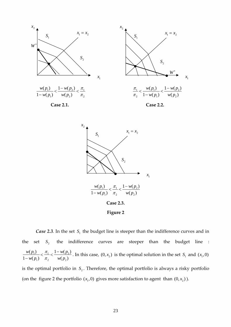
 Case 2.1.            Case 2.2. 

 

 

1 1 2

1 2 2

( ) 1 ( )1 ( ) ( )

w p w pw p w p

ππ

−< <

− 

Case 2.3. 

Figure 2  

 

Case 2.3. In the set  1S  the budget line is steeper than the indifference curves and in 

the  set  2S    the  indifference  curves  are  steeper  than  the  budget  line  : 

1 1 2

1 2 2

( ) 1 ( )1 ( ) ( )

w p w pw p w p

ππ

−< <

−. In this case,  2(0, )x  is the optimal solution in the set  1S  and  1( ,0)x  

is the optimal portfolio  in  2S . Therefore, the optimal portfolio  is always a risky portfolio 

(on the  figure 2 the portfolio  1( ,0)x  gives more satisfaction to agent  than  2(0, )x ). 

 

 

1x

2x

1 2x x=

2S

1S

1x

2x

1 2x x=

2S

1S

W ∗ 1x

2x

1 2x x=

2S

1S

W ∗

24

BIBLIOGRAPHIE Ali M.M. (1977) ‘’Probability and Utility Estimates for Racetrack Betting’’ Journal of Political Economy

85 (4), 803-15.

Allais M. (1953) ’’Le comportement de l’Homme Rationnel devant le Risque, Critiques des Postulats

et Axiomes de l’ École Américaine’’ Econometrica 21, 503-546.

Arzac R. E. et Bawa V. (1977) ‘’Portfolio Choice and Equilibrium in Capital Markets with Safety First

Investors” Journal of Financial Economics 4, 227-288.

Barberis N. et Huang M. (2001) “Mental Accounting, Loss Aversion, and Individual Stock Returns”

Journal of Finance LVI (4), 1247-1292.

Bernoulli D. (1954, Edition originale, 1938) ‘’Exposition of new Theory of the Measurement of Risk”

Econometrica 22, 123-136.

Bernoulli N. (1713 ) ’’Specimen Theoriae Novae de Mensura Sortis’’ Commentarii Academiae

Scientiarum Imperialis Petropolitanae 5, 175-192.

Blume M. et Friend I. (1975) ‘’The asset Structure of Individual Portfolios and Some Implications for

Utility Functions’’ Journal of Finance 30, 585-603.

Broihanne M.H., Merli M. et Roger P. (2004) Finance Comportementale. Economica.

Broihanne M.H., Merli M., Roger P. (2006) ‘’Sur quelques aspect comportementaux de la gestion de

portefeuille’’ (en cours de publication)

Edwards W. (1953) ‘’Probability Preferences in Gambling’’ American Journal of Psychology 66, 349-

64.

Edwards W. (1954) ‘’Probability Preferences Among Bets with Differing Expected Value’’ American

Journal of Psychology 67(1), 56-67.

Edwards W. (1962) ‘’Subjective Probabilities Inferred from Decisions’’ Psychological Review, 69 (1),

109-135.

Fishburn P.C. (1988) ‘’Non Linear Preference and Utility Theory’’ by Weatsheaf Books Ltd.

Fishburn (1978) ‘’On Handa’s New Theory of Cardinal Utility and the Maximization of Expected

Return’’ Journal of Political Economy, 86, 321-324.

Fisher K. et Statman M. (1997) “Investment Advice from Mutual Fund Companies” Journal of

Portfolio Management 24, 9-25.

Friedman M. et Savage L. (1948) ‘’The Utility Analysis of Choices Involving Risk” Journal of Political

Economy 56, 279-304.

Guillen M.F. et Tschoegl A.E. (2002) ‘’Banking on Gambling: Banks and Lottery-Linked Deposit

Accounts’’ Journal of Financial Services Research 21 (3), 219-231.

Jorion P. (1994) ‘’Mean-Variance Analysis of Currency Overlays’’ Financial Analysts Journal 50, 48-

56.

Kahneman D., Slovic P. et Tversky A. (1982) “Intuitive Prediction : Biaises and Corrective

Procedures’’, in Judgment under Uncertainty : Heuristics and Biases, CUP, London.

Kahneman D. et Tversky A. (1979) ’’Prospect Theory : An Analiysis of Decision under Risk’’

Econometrica 47(2),263-291.

Kroll Y., Levy H. et Rapoport A. (1988) ‘’Experimental Tests of the Separation Theorem and the

Capital Asset Pricing Model’’ American Economic Review 78, 500-518.

25

Leonnet J. (1936) ‘’Les loteries d’état en France au XVIIIe et XIXe siècles’’, Paris.

Lopes L.L (1987) ‘’Between Hope and Fear: The Psychology of Risk’’ Advances in Experimental

Social Psychology, 20, 255-295.

Lopes L.L. et Oden G.C. (1999) ‘’The Role of Aspiration Level in Risky Choice: A Comparison of

Cumulative Prospect Theory and SP/A Theory’’ Journal of Mathematical Psychology 43, 286-313.

Markowitz H. (1952) ‘’Portfolio Selection’’ Journal of Finance 6, 77-91.

Pfiffelmann M. et Roger P. (2005) ‘’Les comptes d’épargne associés à des loteries: approche

comportementale et étude de cas’’, Banque et Marchés, sept-oct 2005.

Quiggin J. (1982) ‘’A Theory of Anticipated Utility” Journal of Economic Behavior and Organization 3

(4), 323-343.

Quiggin J. (1993) ‘’Generalized Expected Utility Theory: The Rank-Dependent Model’’ Kluwer

Academic Publishers Group.

Roy A.D. (1952) ‘’ Safety-First and the Holding of Asset’’ Econometrica 20, 431-449.

Shefrin H. (2005). A Behavioral Approach to Asset Pricing. Elsevier Academic Press.

Shefrin H. et Statman M. (2000) “Behavioral Portfolio Theory” Journal of Financial and Quantitative

Analysis 35, 127-151.

Shefrin H.M. et Thaler R.H (1992) ‘’Mental Accounting, Saving, and Self-control’’ Choice Over Time,

éd. G. Loewenstein and j. Elster, New York, NY, Russell Sage Foundation, 287-330.

Thaler R.H. et Jonson E.J. (1990) ‘’Gambling with the House Money and Trying to Break Event: The

Effects of Prior Outcomes on Risky Choice’’ Management Science 36, (6) 643-660.

Tversky A. et Kahneman D. (1992) ‘’Advances in Prospect Theory : Cumulative Representation of

Uncertainty’’ Journal of Risk and Uncertainty 5, 297-323.

Von Neumann J. et Morgenstern O. (1947) “Theory of Games and Economic Behavior” Princeton

University Press (1ed, 1944).

Yaari M. (1984) Risk Aversion without Diminishing Marginal Utility. London School of Economics.

Yaari M.(1987) “The Dual Theory of Choice Under Risk” Econometrica 55, 95-115.

 

 

DULBEA Working Paper Series

2007

N° 07-07.RS Olga Bourachnikova  «Weighting Function in the Behavioral Portfolio

Theory», May 2007. N° 07-06.RS Régis Blazy and Laurent Weill « The Impact of Legal Sanctions on Moral

Hazard when Debt Contracts are Renegotiable », May 2007. N° 07-05.RS Janine Leschke «Are unemployment insurance systems in Europe adapting to

new risks arising from non-standard employment? », March 2007. N° 07-04.RS Robert Plasman, Michael Rusinek, Ilan Tojerow « La régionalisation de la

négociation salariale en Belgique : vraie nécessité ou faux débat ? », March

2007. N° 07-03.RS Oscar Bernal and Jean-Yves Gnabo « Talks, financial operations or both?

Generalizing central banks’ FX reaction functions », February 2007.

N° 07-02.RS Sîle O’Dorchai, Robert Plasman and François Rycx « The part-time wage

penalty in European countries: How large is it for men? », January 2007.

N° 07-01.RS Guido Citoni « Are Bruxellois and Walloons more optimistic about their

health? », January 2007.

2006

N° 06-15.RS Michel Beine, Oscar Bernal, Jean-Yves Gnabo, Christelle Lecourt

« Intervention policy of the BoJ: a unified approach » November 2006.

N° 06-14.RS Robert Plasman, François Rycx, Ilan Tojerow « Industry wage differentials,

unobserved ability, and rent-sharing: Evidence from matched worker-firm

data, 1995-2002»

N° 06-13.RS Laurent Weill, Pierre-Guillaume Méon « Does financial intermediation matter

for macroeconomic efficiency? », October 2006.

N° 06-12.RS Anne-France Delannay, Pierre-Guillaume Méon « The impact of European

integration on the nineties’ wave of mergers and acquisitions », July 2006.

N° 06-11.RS Michele Cincera, Lydia Greunz, Jean-Luc Guyot, Olivier Lohest « Capital

humain et processus de création d’entreprise : le cas des primo-créateurs

wallons », June 2006.

N° 06-10.RS Luigi Aldieri and Michele Cincera « Geographic and technological R&D

spillovers within the triad: micro evidence from us patents », May 2006.

N° 06-09.RS Verena Bikar, Henri Capron, Michele Cincera « An integrated evaluation

scheme of innovation systems from an institutional perspective », May 2006.

N° 06-08.RR Didier Baudewyns, Benoît Bayenet, Robert Plasman, Catherine Van Den

Steen, « Impact de la fiscalité et des dépenses communales sur la localisation

intramétropolitaine des entreprises et des ménages: Bruxelles et sa périphérie»,

May 2006.

N° 06-07.RS Michel Beine, Pierre-Yves Preumont, Ariane Szafarz « Sector diversification

during crises: A European perspective », May 2006.

N° 06-06.RS Pierre-Guillaume Méon, Khalid Sekkat « Institutional quality and trade: which

institutions? which trade? », April 2006.

N° 06-05.RS Pierre-Guillaume Méon « Majority voting with stochastic preferences: The

whims of a committee are smaller than the whims of its members », April

2006.

N° 06-04.RR Didier Baudewyns, Amynah Gangji, Robert Plasman « Analyse exploratoire

d’un programme d’allocations-loyers en Région de Bruxelles-Capitale:

comparaison nternationale et évaluation budgétaire et économique selon trois

scénarios », April 2006.

N° 06-03.RS Oscar Bernal « Do interactions between political authorities and central banks

influence FX interventions? Evidence from Japan », April 2006.

N° 06-02.RS Jerôme De Henau, Danièle Meulders, and Sile O’Dorchai « The comparative

effectiveness of public policies to fight motherhood-induced employment

penalties and decreasing fertility in the former EU-15 », March 2006.

N° 06-01.RS Robert Plasman, Michael Rusinek, and François Rycx « Wages and the

Bargaining Regime under Multi-level Bargaining : Belgium, Denmark and

Spain », January 2006.

2005

N° 05-20.RS Emanuele Ciriolo « Inequity aversion and trustees’ reciprocity in the trust

game », May 2006.

N° 05-19.RS Thierry Lallemand, Robert Plasman, and François Rycx « Women and

Competition in Elimination Tournaments: Evidence from Professional Tennis

Data », November 2005.

N° 05-18.RS Thierry Lallemand and François Rycx « Establishment size and the dispersion

of wages: evidence from European countries », September 2005.

N° 05-17.RS Maria Jepsen, Sile O’Dorchai, Robert Plasman, and François Rycx « The wage

penalty induced by part-time work: the case of Belgium », September 2005.

N° 05-16.RS Giuseppe Diana and Pierre-Guillaume Méon « Monetary policy in the presence

of asymmetric wage indexation », September 2005.

N° 05-15.RS Didier Baudewyns « Structure économique et croissance locale : étude

économétrique des arrondissements belges, 1991-1997 », July 2005.

N° 05-14.RS Thierry Lallemand, Robert Plasman, and François Rycx « Wage structure and

firm productivity in Belgium », May 2005.

N° 05-12.RS Robert Plasman and Salimata Sissoko « Comparing apples with oranges:

revisiting the gender wage gap in an international perspective », April 2005.

N° 05-11.RR Michele Cincera « L’importance et l’étendue des barrières légales et

administratives dans le cadre de la directive ‘Bolkestein’ : Une étude

comparative entre la Belgique et ses principaux partenaires commerciaux »,

April 2005.

N° 05-10.RS Michele Cincera « The link between firms’ R&D by type of activity and source

of funding and the decision to patent », April 2005.

N° 05-09.RS Michel Beine and Oscar Bernal « Why do central banks intervene secretly?

Preliminary evidence from the Bank of Japan », April 2005.

N° 05-08.RS Pierre-Guillaume Méon and Laurent Weill « Can Mergers in Europe Help

Banks Hedge Against Macroeconomic Risk ? », February 2005.

N° 05-07.RS Thierry Lallemand, Robert Plasman, and François Rycx « The Establishment-

Size Wage Premium: Evidence from European Countries », February 2005.

N° 05-06.RS Khalid Sekkat and Marie-Ange Veganzones-Varoudakis « Trade and Foreign

Exchange Liberalization, Investment Climate and FDI in the MENA »,

February 2005.

N° 05-05.RS Ariane Chapelle and Ariane Szafarz « Controlling Firms Through the Majority

Voting Rule », February 2005.

N° 05-04.RS Carlos Martinez-Mongay and Khalid Sekkat « The Tradeoff Between

Efficiency and Macroeconomic Stabilization in Europe », February 2005.

N° 05-03.RS Thibault Biebuyck, Ariane Chapelle et Ariane Szafarz « Les leviers de contrôle

des actionnaires majoritaires», February 2005.

N° 05-02.RS Pierre-Guillaume Méon « Voting and Turning Out for Monetary Integration:

the Case of the French Referendum on the Maastricht Treaty », February 2005.

N° 05-01.RS Brenda Gannon, Robert Plasman, Ilan Tojerow, and François Rycx «

Interindustry Wage Differentials and the Gender Wage Gap : Evidence from

European Countries », February 2005.

Apart from its working papers series, DULBEA also publishes the Brussels Economic Review-Cahiers Economiques de Bruxelles. Aims and scope First published in 1958, Brussels Economic Review-Cahiers Economiques de Bruxelles is one of the oldest economic reviews in Belgium. Since the beginning, it publishes quarterly the Brussels statistical series. The aim of the Brussels Economic Review is to publish unsolicited manuscripts in all areas of applied economics. Contributions that place emphasis on the policy relevance of their substantive results, propose new data sources and research methods, or evaluate existing economic theory are particularly encouraged. Theoretical contributions are also welcomed but attention should be drawn on their implications for policy recommendations and/or empirical investigation. Regularly the review publishes special issues edited by guest editors.

Authors wishing to submit a paper to be considered for publication in the Brussels Economic Review should send an e-mail to Michele Cincera: mcincera@ulb.ac.be, with their manuscript as an attachment. An anonymous refereeing process is guaranteed.

Additional instructions for authors and subscription information may be found on the Brussels

Economic Review’s website at the following address:

http://homepages.vub.ac.be/~mcincera/BER/BER.html

Brussels Economic Review

University of Brussels DULBEA, CP140

Avenue F.D. Roosevelt, 50 B-1050 Brussels

Belgium

ISSN 0008-0195