Document de travail de la série Etudes et Documents E 2002

CERDI, Etudes et Documents, E 2002.14

Document de travail de la série Etudes et Documents

E 2002.14

Currency boards: are they as strong as they look?

Jean-Louis COMBESa, Romain VEYRUNE*b

a CERDI, University of Auvergne, France b CERDI, University of Auvergne, France

June 2002, 26 p. * Corresponding author. Tel : +33(0) 4-73-17-74-00; Fax: +33(0) 4-73-17-74-28 E-mail address: [email protected]


Currency boards: are they as strong as they look?

Abstract Since Krugman 1979, we know that the fixed exchange rate regimes have a propensity to fail because governments are unable to commit simple monetary rule in order to avoid divergence between base money supply and reserve variations. The currency boards (CB) propose a radical solution: an institutional rule linking base money and reserve. In this context, how to explain the failure of the Argentina CB? We test, in a co-integration model adapted for panel data, the efficiency of the CB rule to run the monetary policy. We conclude that in some situations, as Argentina bi-monetarism, the monetary policy could become inoperative. Keywords: Currency Boards, endogenous money supply, Panel unit root test, Panel co-integration model, Argentina. JEL Classification: C22, C23, E51, E52, F31, F32, F33. Résumé Depuis les travaux de Krugman nous savons que les régimes de change fixe ont une forte propension à s'effondrer. Cette faiblesse tiendrait à l'incapacité des gouvernements à respecter la règle du jeu d'un régime de change fixe : c'est-à-dire empêcher les déviations significatives entre la base monétaire et les réserves de change. Les caisses d'émission proposent une solution radicale : établir un lien institutionel entre la base monétaire et les réserves. Dans ce contexte comment expliquer l'échec argentin ? Pour apporter un élément de réponse, nous essayons, grâce à un modèle de cointégration adapté au panel, de tester l'efficacité de la règle des CB pour conduire la politique monétaire. Les résultats de ce test nous incitent à penser que certaines situations, comme le bi-monétarisme argentin, peuvent rendre la politique monétaire des Caisses d'émission inopérante.

mots clé : Caisses d'émission, offre de monnaie endogène, test de racine unitaire en panel, modèle de co-intégration en panel, Argentine.


Introduction.

Fixed exchange rate regimes are known to have an important propensity to fail. Since

Krugman (1979), we have some evidences about the monetary reasons for their failures.

Krugman demonstrates that a deviation between monetary base and foreign assets conduct to

the collapse of the regime. Without an institutional and clear link between the two aggregates,

the fixed exchange rates suffer a fatal lack of credibility, which greatly concurs to the check

of the regime. The Krugman explanation has the advantage to offer only monetary

explanations to the weakness of the regime.

One way to vanish the lack of credibility of fixed exchange rates and to solidly

establish the trust in the regime could be to promote a clear institutional link between

monetary aggregates and foreign currency aggregates. The currency board has suggested a

solution for a long time: foreign currencies as the unique counterpart of base money. Foreign

currencies are a secure, liquid and always available counterpart; and the control of base

money constitutes an efficient tool to regulate the money and the credit evolution. In effect,

historically, few indeed no orthodox currency boards have known a failure. However, the

Argentina bankruptcy and its currency board abandon recently lower the credibility of this

kind of regime: Currency boards are they as strong as they look?

In order to check this assumption, we test the convergence hypothesis between base

money and external position in a currency board regime with a co-integration model adapted

for a panel data structure. The main idea is to check the compliance with the rule for the

whole currency boards experiences in the 90's (five countries in our panel: Argentina,

Bulgaria, Hong Kong, Estonia and Lithuania) and to evaluate the degree of heterogeneity of

the panel. Could a country engaged in a currency board, for example Argentina, significantly

deviates from the panel interpretation of the rule for a soft compliance?

We recall, in a first section, how the currency boards could improve the credibility of

the fixed exchange rates in a Krugman type model and we present the reason why they may

fail to achieve their mission. In a second section, we present our econometric tests.

3


1. The fatal death of fixed exchange regimes and currency boards.

In a currency board regime the base money supply is endogenous, and this feature

greatly improves the credibility of the regime. Before explaining why the base money supply

can be consider as endogenous, we recall the fundamental weakness of fixed exchange

regimes as exposed by Krugman (1979). In a last step, we briefly evoke the implications of an

endogenous base money supply on monetary policy.

Krugman observes frequent failures of government to maintain a fixed parity1. This

statement holds even if the government is able to get some re-fund. In that case, the

government can compensate the reserve depletion and restore the confidence in order to avoid

the crisis. However, this strategy is linked to the capacity of getting re-fund, and this capacity

vanishes over the time2.

The survival of a fixed exchange rates regime is determined by external accounts. A

lack of foreign reserves implies that the monetary authorities are no longer able to comply

with their obligation of converting their money in foreign currency at a fixed exchange rate.

Thus, the basic rule to safeguard such a regime is to connect the domestic-inflation to the

anchor-inflation, in order to avoid any competitiveness losses which compromise current

account. Insofar, as excessive money issue causes inflation, the domestic money supply has to

follow the anchor money supply. In case of excess inflation, the current account deficit leads

to a depletion of reserve in fixed exchange system. If the country respects the rule of the

game, this depletion should imply a reduction of money supply and, thus, a reduction of

inflation that vanishes current account deficit and vice versa. Consequently, an automatic

mechanism adjusts the money supply to reserve variations in order to comply with fixed

exchange rate rules.

1 Krugman (1979) notes that: “at a fixed exchange rate the government’s reserves gradually decline. Then at some point, generally well before gradual depletion of reserves would exhaust then; there is a sudden speculative attack that rapidly eliminates the last of reserve. The government then becomes unable to defend exchange rate any longer” 2 To quote Krugman (1979) again: “it sometimes happens that the government is able to weather the crisis by calling on some kind of secondary reserves: it draws on its gold tranche or negotiates emergency loans. At this point, there is a dramatic reversal, the capital that as just flowed out returns, and the government’s reserves recover. The reprieve may only be temporary. Another crisis may occur, which will oblige the government to call on still further reserves. There may be a whole sequence of temporary speculative attacks and recoveries of confidence before the attempt to maintain fixed exchange rate is finally abandoned.”

4


However, in Krugman model, the government has not enough incentives to respect the

basic rule of the game. Coping with external shocks or financing budget deficit incites the

government to issue money without any respect of foreign reserve amount. Indeed, a time

inconsistency appears between the rate of growth of base money and the obligations of fixed

exchange rate regimes. Investors aware of this inconsistency do not trust the government

announcements. Most traders forecast the abandon of the fixed exchange rate, i.e. potential

gains in holding foreign assets. This speculative movement exhausts the central bank foreign

reserve as soon as the regime becomes less credible. The speculation accelerates the end of

the fixed exchange rate regime.

A legal rule can institutionalize the link between reserve and money supply, and can

dismiss the government discretion. In that case, the fixed exchange rule and the anti reserve

depletion mechanism can hold. Trust in the regime is guarantied and, thus, the credibility is

restored. Such an institutional fixed exchange rate regime avoids the fatal death described by

Krugman. That is exactly what the currency board regime looks for. In a currency board

system, the law forbids explicitly all the base money counterparts different from foreign

liquid assets. In the central bank accounts the short-term liability of the bank (essentially the

base money) are equal to the foreign reserve. The availability of liquid foreign assets gives a

guarantee to internal and external domestic assets holders of satisfying their exchange demand

at a fixed and known rate. In addition, the limited central bank counterpart regulates the base

money issue. Such a regulation of an essential monetary aggregate powerfully influences the

monetary policy in a low inflation bias.

In effect, the currency boards have known lasting experiments. Historically, they have

been widely spread in the developing countries during the XIXth and the first part of the XXth

century. At the heyday of the regime, it was in function in seventy countries around the world.

They provide a stable fixed exchange rate regime and the failures have been very scarce,

indeed none. Abandoned for political more than economical reasons in the 1950-60’s, they

have done a noticed come back in the 90’s. Countries in great monetary turmoil as Argentina

and Bulgaria use the rule to stabilizing quickly their economy and the results have been quite

efficient. Estonia and Lithuania use the rule to issue a credible new currency the day after

their independence. The new issues successfully integrated the world of the international

currencies. The oldest currency board, Hong Kong, maintains the regime in order to stay a

solid international financial place. In the turmoil of the 1997 Asian crisis, the Hong Kong

dollar kept its exchange rate pegged with the united states dollar. At a first sight, the currency

5


board seems to be an efficient monetary tool for developing countries. However, recently, the

Argentina bankruptcy questions the evidence of currency board monetary success: how a

regime, which is supposed to handle a great quantity of foreign reserve, could let a country in

foreign debt suspension of payments?

The collapse of Argentina recently lowers the credibility of currency board. In

particular, it puts in doubt the truth telling of the currency board arrangement. The strength of

the currency board rule is that it looks like an identity in the central bank accounts. However,

the 90’s currency boards are qualified as non-orthodox because they abandon certain

characteristics of the genuine ancestral currency boards. The orthodox currency board had a

strict definition of the rule: they could not hold foreign reserve more than 100% of the base

money. They excluded the possibility widely used in new currency boards of holding excess

foreign reserve in order to generate rooms to some monetary policy interventions opposite to

the “currency spirit”. In the present currency boards (Argentina (1991), Estonia (1992),

Bulgaria (1997) and Lithuania (1994)), the law allows some regulation of credit and bank

activities. However, the central bank chart generally stipulates limitations to the use of these

tools. These limitations correspond to amendments of the former central bank chart

empowered in order to respect the currency or convertibility acts, which are the true laws

establishing the Currency Board system. The only case where the central bank chart (and its

available instruments) is fully altered is the case of the Bulgarian National Bank.

The following quadrant is an extract of the Argentina laws establishing a currency

board. Argentina is the oldest modern currency board, which inspired especially Estonia and

Lithuania currency boards. Seven extracts from the laws establishing currency board in

Estonia, Lithuania and Bulgaria are presented in Appendix A.

6


Argentina The law 12.155 (May 31, 1935) empowered the Central Bank of Argentina Republic (CBAR). In effect, this law ended a "caja de conversion" composed of various monetary and banking institutions, functioning closely to a currency board, and created a centralized body functioning as a classic central bank. However, the new body kept certain autarchy, for example a great part of its capital remained private. This organic law has been altered several times to improve the discretionary capacity of the institution and to reduce its independence. We could notice especially the decree 8.505 (1946) that nationalized the central bank, and the law 20.520 (1973), which imposes that the monetary policy have to follow the government policy. These laws also increased the discretionary abilities of the central bank. The convertibility act (law 23.928, (1992)) completely changed the monetary authorities nature. We quote the main articles below: Article 1: The convertibility between the austral and the United stated dollar is

established at a rate of 10.000 austral per dollar. (The year after, the austral was replaced by the peso at a rate of 10.000 austral for a new peso).

Article 1bis (2001): the convertibility between the peso and the united state dollar is

established at the rate of 1 United stated dollar and 1 European Union Euro. Article 2: the CBAR shall sell the foreign exchange required for conversion operation

at the rate established by Article 1. Article 4: the freely available reserves of the CBAR in gold and foreign exchange shall

always be equivalent to at least one hundred percent of the monetary base. These three articles would suffice to establish, in effect, the currency board. However, the republic of Argentina always disposes of a central bank, whose chart (BCRA’s chart, law 24,144 (1992)) stipulated :

The primary and essential mission of the Central Bank is to preserve the value of the national currency, in order to secure the function of money as value of reserve, unit of account and instrument of payment (article 3). The central bank shall not be subject to any order, suggestion or instruction given by the national executive power.

The new chart institutes the independence of the BCRA, and considerably reduced its discretionary power. However, we notice that an important number of central bank traditional prerogatives persist :

The central bank chart retains the possibility to rediscount or refinance the commercial bank in difficulties of solvency (article 17.1), but strictly limits the period and the amount per institution (article 17.2). The period is limited to 30 days and to the amount of the equity capital.

The central bank could operate certain open market operations with its excess resources (excess of foreign reserves on base money) (article 18).

7


The commercial banks have to fill deposit on the central bank account. The reserve requirement on these accounts is determined by the central bank. The reserve requirement of the central bank itself comes from the convertibility act (100% of the money base in foreign reserves) (article 28). The supervision of the banking system recovers from a superintendent, mainly empowered of issuing licenses and authorizations to practice a financial activity (article 34).

The legacy of the central bank system to the currency board is important. The currency board has various tolls to regulate the credit and to supervise commercial banks. However, these tolls are available in strict bounds defined by the convertibility act. In fact, the monetary authorities are much more ruled by the Convertibility act, which fixes the resource available for the monetary authorities, than by the central bank chart, which only gives marginal capacity of action on credit.

In spite of the tight arrangement, the government and the central bank have some

rooms to deviate from the strict application of the rule. The motivations to deviate for a weak

government could be strong.

Even if the government is not able or unwilling to soften the rule, people themselves

could worsen the rule mechanism. Indeed, the adjustment, which insures the viability of fixed

exchange rate, supposes that the rule makes base money very reactive to exit/entry of foreign

currency in the country. However, the change Money-currency is never instantaneous. People

can hold foreign currencies (currency retention) or it can exist delays less or more important

due to technical factors. The technical reasons are simply the time taken by the traders and the

banking sector to effectively done the change. Which factors can influence the delays and the

holding of currencies? For the delays, we could imagine that the technical reasons are quite

invariant. On the contrary, the retention of currencies would be influenced by the trust in the

regime and the confidence in the future of the national economy. More specifically in the case

of Argentina, the monetary regime was bi-monetarist, the dollar and the peso were both legal

tenders. By the way, Argentina shared its base money between the peso base money produced

by the CB and the imported dollar base money privately managed, meanly by banks and

traders. The imported base money was entirely independent from the CB rule. We could

suppose that if the constraint becomes tighter, the incitement to use dollar would be higher,

that to say people hold a greater part of their private local deposits in dollar. In effect, people

worry by the long recession and mistrustful about their institutions used the possibility to hold

deposits in dollar to protect their assets, by the way, the base money, is to say monetary

8


policy, become less sensitive to external account variations and the adjustment mechanism

disappear. When the crisis become really critical, in order to avoid the deflation due to the

shortage of liquidity, some federal bodies (federal treasuries) issue substitute base money as

patacondes or argentino which contribute to make the legal base money issued by the CB less

sensible, indeed rigid, to external account.

The skirting of the central bank by an important part of the private sector, as the will

of the government to soften the rule, could make the regime inoperative to implement an

efficient external account adjustment mechanism likely to improve the survival of fixed

exchange rate. In order to test if the currency boards are as strong and honest as they look, we

evaluate, in the next section, the standard currency board behavior in the group of five

countries implementing this regime in the 90’s. The average effective implementation of the

rule is used as a benchmark to stress the experiments that significantly deviate from the CB’s

rule commonly used.

2. Empirical test on long run and dynamic relation between base money and external position.

In this section, we test the link previously supposed between base money supply and

external reserve. The experiments of institutional monetary rule regime on a long period of

time are not really numerous. So we use an unbalanced panel data structure with 5 countries

(Argentina 1991-2002, Estonia 1992-2002, Lithuania 1994-2002, Bulgaria 1997-2002 and

Hong-Kong 1990-2002).

Formally, we can write a long run relation between base money and external balance:

M0i,t = βi.Xi,t + εi,t (1)

with Xi,t = Ci + Σtj=t0,iBGi,j.

M0i,t, is the base money at time t for the country i. It is the part of money aggregate on

which the monetary authorities have a monopoly on issue. The series are provided by the

international financial statistics (IFS), issue December 2001. We use the ratio between the M0

9


aggregate and the GNP. Such a ratio permits to have a more homogenous indicator to

compare M0 variations between countries3.

Xi,t = Ci + Σtj=t0,iBGi,j represents the net currency balance or exterior position of the

country i at time t. Ci are the foreign available reserve at the beginning of the system and

Σtj=t0,iBGi,j are the cumulated overall balances BGi,t , since the begning of the system is in t0,i

in each country. The data on reserves and overall balances are extracted from IFS December

2001. We use the ratio of the external position to the GNP 4. This aggregate represents the

stock of foreign assets standing in the country at each date. This evaluation of foreign assets is

different from the foreign asset available for the currency board. Indeed the only a part of the

stock of foreign assets belongs to the board.

εit is the usual disturbance term for the country i at time t.

βi is the coefficient of the long term relation between base money and the stock of

foreign assets. The currency board principle well defines the relation between base money and

the fraction of foreign asset belonging to the board. Indeed, in a strict 100% backing rule, the

coefficient linking base money and board foreign asset must be equal to 1. However, the

exceptional rule-ratio manipulations and excess reserve practices are able to slightly deviate

the coefficient from one. Moreover, we don't test the relation between the fractional currency

board reserve and the base money, but the relation between the total external position of the

country and the base money. The board handles only a fraction of the total foreign asset and

doesn't clearly define the relation that we estimate. We assume thus that the relation between

the two aggregate must be high, that to say close but less than 1, and strongly significant.

The unit of time is the quarter. In a first time, we test the order of integration of M0

(base money), and of the country external position, with a specific unit root test adapted for

panel: Maddala and Wu (1999) based on the Elliot, Rothenberg and Stock (1996) statics. In a

second time, with the Choi (2001) method, we test the co-integration hypothesis in our model.

In a third time, we provide an estimation of the long run relation between base money and

external position assumed in currency board regime. Finally, we highlight the short term

dynamic, using the Engle Granger two steps method.

.

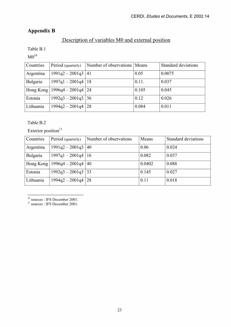
3 Annex 2: The table A.1 gives some statistical information about M0. 4 Annex 2: The table A.2 gives some statistical information about the exterior position.

10


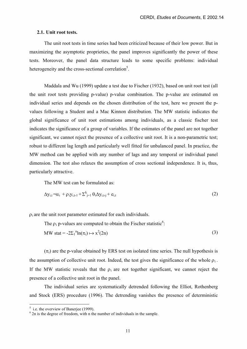
2.1. Unit root tests.

The unit root tests in time series had been criticized because of their low power. But in

maximizing the asymptotic proprieties, the panel improves significantly the power of these

tests. Moreover, the panel data structure leads to some specific problems: individual

heterogeneity and the cross-sectional correlation5.

Maddala and Wu (1999) update a test due to Fischer (1932), based on unit root test (all

the unit root tests providing p-value) p-value combination. The p-value are estimated on

individual series and depends on the chosen distribution of the test, here we present the p-

values following a Student and a Mac Kinnon distribution. The MW statistic indicates the

global significance of unit root estimations among individuals, as a classic fischer test

indicates the significance of a group of variables. If the estimates of the panel are not together

significant, we cannot reject the presence of a collective unit root. It is a non-parametric test;

robust to different lag length and particularly well fitted for unbalanced panel. In practice, the

MW method can be applied with any number of lags and any temporal or individual panel

dimension. The test also relaxes the assumption of cross sectional independence. It is, thus,

particularly attractive.

The MW test can be formulated as:

∆yi,t =αi + ρiyi,t-1 + Σkj=1 θi∆yi,t-j + ei,t (2)

ρi are the unit root parameter estimated for each individuals.

The ρi p-values are computed to obtain the Fischer statistic6:

MW stat = -2Σ1nln(πi) a x2(2n) (3)

(πi) are the p-value obtained by ERS test on isolated time series. The null hypothesis is

the assumption of collective unit root. Indeed, the test gives the significance of the whole ρi .

If the MW statistic reveals that the ρi are not together significant, we cannot reject the

presence of a collective unit root in the panel.

The individual series are systematically detrended following the Elliot, Rothenberg

and Stock (ERS) procedure (1996). The detrending vanishes the presence of deterministic

5 i.e. the overview of Banerjee (1999). 6 2n is the degree of freedom, with n the number of individuals in the sample.

11


trend in individual series likely to weaken the ADF test. Our series on money and external

accounts are known to be usually subject to deterministic trend. This alteration of the series

greatly improves the ADF power7.

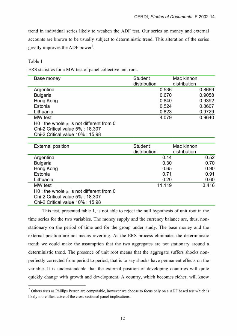
Table 1

ERS statistics for a MW test of panel collective unit root.

Base money Student distribution

Mac kinnon distribution

Argentina 0.536 0.8669Bulgaria 0.670 0.9058Hong Kong 0.840 0.9392Estonia 0.524 0.8607Lithuania 0.823 0.9729MW test H0 : the whole ρi is not different from 0 Chi-2 Critical value 5% : 18.307 Chi-2 Critical value 10% : 15.98

4.079 0.9640

External position Student

distribution Mac kinnon distribution

Argentina 0.14 0.52Bulgaria 0.30 0.70Hong Kong 0.65 0.90Estonia 0.71 0.91Lithuania 0.20 0.60MW test H0 : the whole ρi is not different from 0 Chi-2 Critical value 5% : 18.307 Chi-2 Critical value 10% : 15.98

11.119 3.416

This test, presented table 1, is not able to reject the null hypothesis of unit root in the

time series for the two variables. The money supply and the currency balance are, thus, non-

stationary on the period of time and for the group under study. The base money and the

external position are not means reverting. As the ERS process eliminates the deterministic

trend; we could make the assumption that the two aggregates are not stationary around a

deterministic trend. The presence of unit root means that the aggregate suffers shocks non-

perfectly corrected from period to period, that is to say shocks have permanent effects on the

variable. It is understandable that the external position of developing countries will quite

quickly change with growth and development. A country, which becomes richer, will know

7 Others tests as Phillips Perron are computable, however we choose to focus only on a ADF based test which is likely more illustrative of the cross sectional panel implications.

12


an increase of its external position. This increase will be deeply influenced by the erratic

variations of the growth rate, and by the also erratic variations of the political preference for

inward or outward looking development.

2.2. Co-integration test.

Choi (2001) proposes a comprehensive co-integration test. It is the extension for panel

data of unit root test based on residual from the Engle Granger first step. The method consists

in determining the order of integration of the estimated residual of the long run relation: εit

(equation 1).. It is close to the previously presented unit root MW (1999) test. It consists in a

combination of residual unit root test p-values calculated for isolated time series. In effect, it

follows the same procedure and the same critical value as MW (1999). It is, thus, easy to

compute and presents the same advantage of the MW test. Especially, it requires few

assumptions on sample and individuals nature (cross sectional heterogeneity, cross sectional

independence) and has high power8.

The result are presented in table 2. We should admit that one time series included in

our panel is quite short to report an ADF test really strong; the other time series are good

enough to be reliable. The test is not able to reject the hypothesis of co-integration.

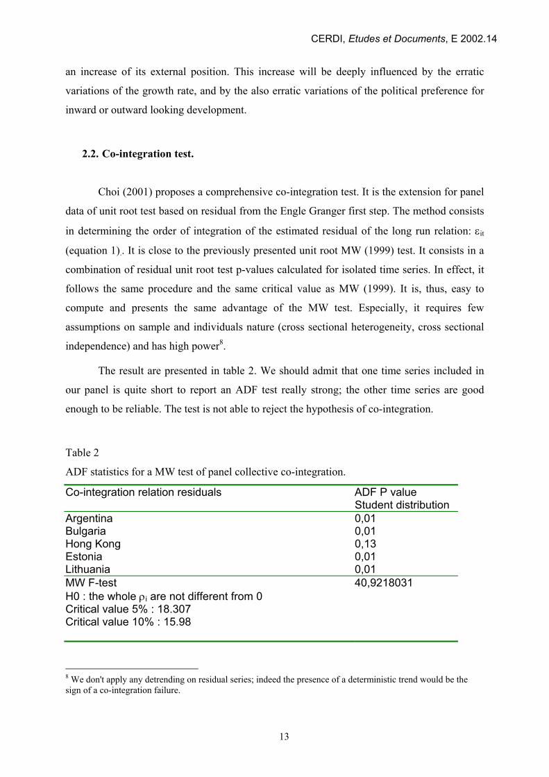
Table 2

ADF statistics for a MW test of panel collective co-integration.

Co-integration relation residuals ADF P value Student distribution

Argentina 0,01 Bulgaria 0,01 Hong Kong 0,13 Estonia 0,01 Lithuania 0,01 MW F-test H0 : the whole ρi are not different from 0 Critical value 5% : 18.307 Critical value 10% : 15.98

40,9218031

8 We don't apply any detrending on residual series; indeed the presence of a deterministic trend would be the sign of a co-integration failure.

13


Co-integration between base money and foreign assets is theoretically expected, the

test supports the theoretical hypothesis. Indeed, the statistic doesn't stress the presence of unit

roots in the co-integration long-run relation residuals.

2.3. Model specification: Long-term representation.

The currency board systems give us the luck to establish a clear bi-variate co-integration

relation. The two integrated variables are the base money and the external position. The long

run relation, Engle Granger first step, could be described in three ways as follows:

(1) All the countries across the panel are supposed to have the same behaviors (to be the

same), thus the coefficient and the intercept are homogenous between individuals, i.e equation

4.

M0i,t = α + δ.t + β.Xi,t + εi,t (4)

(2) The panel is known to be heterogeneous. In such a panel, we cannot assume a perfect

homogeneity in intercepts and slopes across individuals, i.e. equation 5.

M0i,t = αi + δi.t + βi.Xi,t + εi,t (5)

(3) In a CB's case, the monetary authorities intervention means are ruled, we can, thus,

suppose the individual behaviors to be quite homogenous and slopes to be close. Our

specification, inspired from Pedroni (1995), supposes and tests the homogeneity of the slope

βi constant among countries. However, we keep the individual specific intercepts to allow for

certain heterogeneity among individuals due to the great diversity of country types in our

sample, except the use of CB's system. In addition, we introduce individual specific time

trend in order to control for trend likely to be present in monetary aggregates. The

sustainability of the exchange rate regime as exposed formerly supposes a marginal or

negative time trend, that to say δi non significant or negative, i.e. equation 6.

M0i,t = αi + δit + β.Xi,t + εi,t (6)

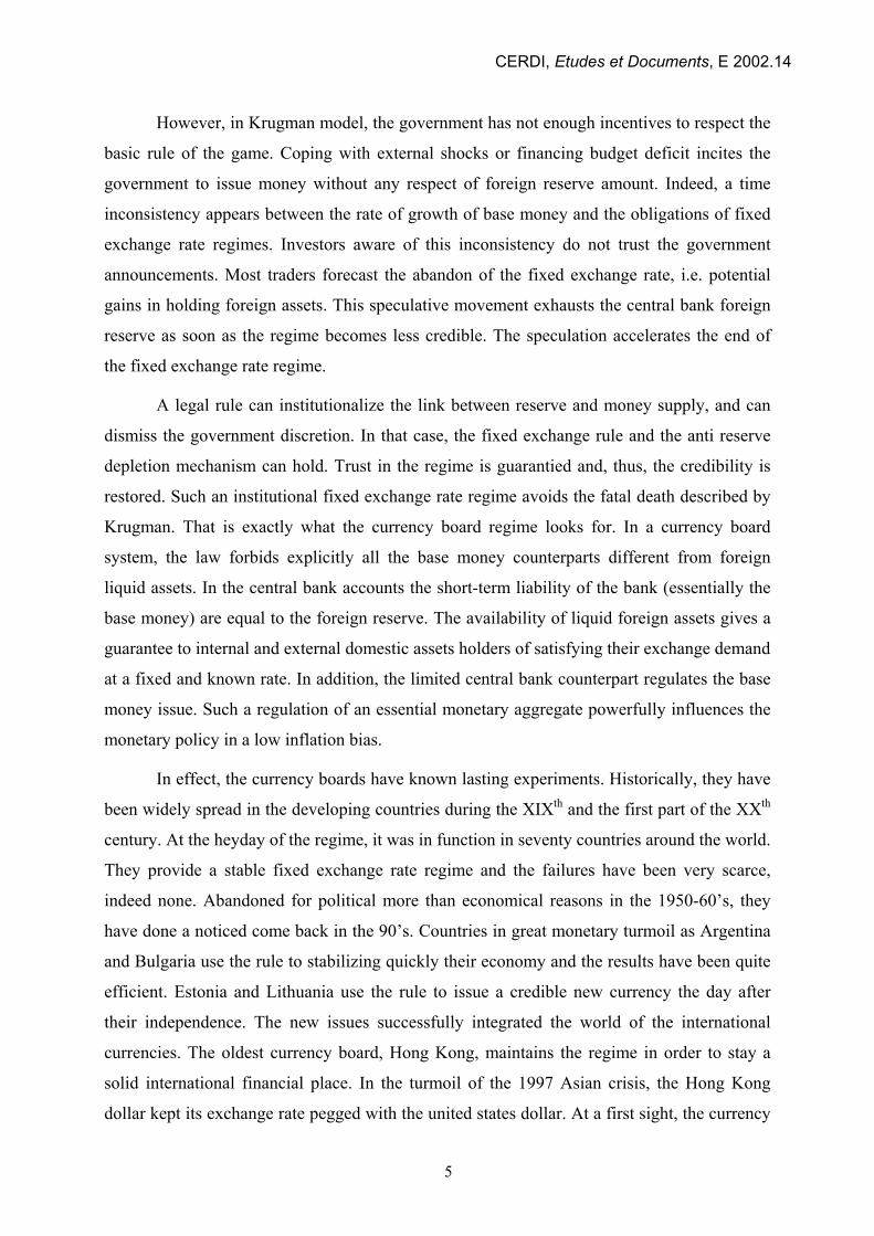
The following chart illustrates the chosen modelisation of the currency board rule.

Three scenarios are exhibited. The first scenario assumes the convergence between base

money and external account toward a stable long run relation as illustrated by B. As previouly

14


specified, the line B has a slope positive, constant, close to one but always inferior to the

unity. An intercept assumes that the base money would never be null, even if the external

position is null. The panel specification allows this intercept two be different across countries,

for the ease of the representation we draw only an unique intercept. The B line constitutes a

boundary. Above the line, the A case, the base money/external position ratio grows at a faster

rate than the long run relation, thus the monetary policy diverges from the rule and the fixed

exchange rate regime becomes unsustainable. Below the B line, the ratio base money/external

position grows at a rate inferior or equal to the long run relation, the regime is viable. A

positive and significant deterministic time trend or a slope superior to the unity corespond to

the A scenario. Non significant or negative trends and a slope equal or inferior to one

correspond to the viable scenario B and C.

base money.

Fig. 1. Convertibility scenario in a Currency Bo

15

A

B

C

45°

External position.

ard context.


Table 3

Engle Granger long-term relation. Equation 6.

Number of observation = 141 Within estimator R-sq:0.93 Coefficient. p-value

Xi,t 0.51 0.000 Argentina -0.00063 0.013 Bulgaria 0.00283 0.026 Hong Kong -0.00880 0.762 Estonia 0.00102 0.190

Individual time specific effect

Lithuania 0.00022 0.754 Constant 0.02766 0.000 (fixed effects) F(4. 130) = 2.43(0.01)

The long run estimation fits well with the model assumption, i.e. table 3 : the slope is

strongly significant, positive and inferior to one. Consequently, we conclude that it exist on

the long run and across the panel a stable base money / external position relation. The

estimated coefficient which sizes 0.51, indicates that the base money is undersensitive to the

external position variations. Indeed, only a part of the external position are recorded in the

currency board accounts, the remainder is kept by the public or by the banks. The external

flux which impacts the central bank balance sheet are, thus, the lone likely to change the

monetary policy, that to say to modificate the base money stock. The trends are, in a great

majority of cases, no significant or negative. The lone positive significant trend concerns

Bulgaria one of the shorter time series. But, in this case, we notice that the estimated trend is

really low, or even marginal.

2.4. Homogenous short-term dynamic.

We think that during each period, due to various internal and external shocks, the base

money will tend to deviate from its long-term relation with the country external position,

defined in equation 6. However, in contrary to other monetary regimes, the CB's system

forecasts an automatic mechanism to send back the base money to its long run

correspondence with CB external assets (proxy of the country external position). This

mechanism defines an error correction model close to that presented by Engle and Granger

(EG) (1987). The EG method has often been criticized, above all it is really non-performing

on small sample. It is also particularly sensitive to the presence of omitted variables. The rule-

16


based model may bring a correct specification moreover, the use of a fixed effects model

catches the effect of individual specific and time invariant characteristics9.

The dynamic short run relation could be written as:

∆M0i,t = ai + b.∆Xi,t + σ.(εi,t-1) + ei,t (7)

b gives the dynamic between the base money supply and the overall balance. b is

supposed constant across countries. σ is the coefficient of the error correction term. It gives

the rate of convergence of the model to its long-term equilibrium. If σ is significantly -1<σ<

0, the model is convergent to the long run equilibrium defined in (6). If σ is not different from

0, the model would not converge to an equilibrium. According to the Granger theorem, co-

integrated variables always converge. A significant convergence coefficient σ is, thus, the

indicator of a correct co-integration specification.

Table 4

Engle Granger short run dynamic. Equation 7

Number of observation =122 Within estimator R-sq:0.72 Coef. P-Value

∆xi,t 0.44 0.000 (εi,t-1) -0.82 0.000 Constant 0.00053 0.74

(fixed effects) F(4,115) =2.3(0,05)

The convergence coefficient (table 4) is strongly significant, that supports our

hypothesis of co-integration and also confirms the good feature of the EG model. The rate of

convergence is quite high, from a quarter to another, more than 3/4 of the divergence from the

long-term equilibrium is corrected. The monetary policy will, thus, quickly react to any

modification of the external position. In less than 6 months, the base money will be adjusted

to its long run relation with the stock of external assets available in the country.

9 Others methods have been developed in the area of co-integration as for example the one step procedure or the Henry method. They both present bias consisting in lagged dependent variable endogeneity in a panel specification. Assessing respective bias of the methods, we prioritize the EG procedure.

17


2.5. Heterogeneous short-term dynamic.

Finally, we cross the correction error term and the country dummy variables to test for

some panel heterogeneity in the error correction term σ (table 5). So we estimate the

following model:

∆M0i,t = ai + b.∆Xi,t + σi.(εi,t-1) + ei,t (8)

Table 5

Error Correction Term homogeneity.

Number of observation =121 Within estimator R-sq: 0.74 Coefficient. p-value ∆xi,t 0.43 0.000 (εt-1) Argentina -0.20 0.020 (εt-1) Bulgaria -0.99 0.013 (εt-1) Hong Kong -0.73 0.013 (εt-1) Estonia -0.81 0.009 (εt-1) Lithuania -1.01 0.016 Constant 0.006 0.321

In a perfect homogeneity context the entire coefficient estimated for the error

correction term would have been the same. However, the individual specific effects do not

seem to be perfectly neutral. In particular, Argentina significantly diverges from the other

countries in the panel and reveals a less efficient convergence. This divergence can be

explained by a “soft” interpretation of the rule or by the people abandon of the peso. In

particular, another reflection has to be carry out about the role played by the substitutes of

money issued by federal bodies at the end of the regime. They have, probably, contributed to

significantly lower the sensibility of the base money to external accounts, and to lower the

sensibility of money and credit to the board base money, that to say the official peso issued by

the board.

In order to test further the panel heterogeneity, we implement another test. We add to

the general error correction term and individual specific error correction term for each

individuals.

∆M0i,t = ai + b.∆Xi,t + σ(εi,t-1)+ σi.(εi,t-1) + ei,t (9)

18


We estimate the equation (9) with σi.(εi,t-1), the country specific error correction for

one country (i), and σ(εi,t-1), the general error correction term for all the panel. We repeat the

process for each country of the panel. By the way, we can estimate the differential impact of

each country on the panel co-integration short term relation.

Table 6

Country specific effect.

fixed effect estimation Panel ECT Country specific ECT Argentina -092** 0,7** Bulgaria -0,79** -0,2 Hong Kong -0,84** 0,12 Estonia -0,81** 0,0014 Lithuania -0,72** -0,46**

The error correction term is significant for any control; that confirms the coherence of

our currency boards panel. However, we notice two groups of countries. On one hand,

Estonia, Bulgaria and Hong Kong for which the control is not significant, that means that

theses three countries have not specific effect different from the remainder of the panel. In

particular Estonia appears to be the currency board standard of the panel. Its control specific

makes absolutely no changes. In another hand, Lithuania and Argentina significantly break

the homogeneity of the panel. Lithuania converges toward the long-term equilibrium quicker

than the remainder of the panel (40% quicker). On the contrary Argentina converge much

more slowly toward the equilibrium than the rest of the group. This divergence reveals a

"soft" implementation of the rule likely to disrupt the regime.

3. Conclusion.

Our tests conclude that the currency board regime permits, in most of case, a rapid

convergence between base money and external account. This convergence had been stressed

as the condition of viable fixed exchange rate regime. In addition, the behaviors of the

currency board regimes are quite close. The monetary policy of all countries, honestly

adopting a currency board, converges toward the same result.

19


However, some divergences are empirically noted. Government and board keep some

rooms likely to tighten or to soften the constraint imposed by the rule. In addition, the regime

stays dependent from the trust of people and of the state good governance. In the majority of

cases no significant deviations in opposite to the rule are noticed. The lone case, which

exhibits a clear deviation from the rule, is the case of Argentina. The Argentinean case is a

relevant example of board's limits. Indeed, Argentina did not seem able to accept the currency

board constraints. Some internal characteristics make the internal cost, in terms of

unemployment for example especially high and painful. Consequently, the government and

the board used all rooms available to soften the rule. People used to handle dollar and peso,

both national legal tender, accumulated dollar position out of the rule regulation. At the end of

the system, symptomatic of the government no cooperation, some federal bodies issued notes

as central bank money substitute. These issues contributed to ended the system.

Appendix A Laws and Acts ruling monetary authorities in some CB regime.

Estonia The first Estonian central bank born with the first Estonian national independence in 1919. It was an active body disposing of great discretionary powers. However, in order to permit fixed exchange rate with the German mark, it reforms its status to approach a currency board system based on a gold standard (1926). With the soviet invasion the bank of Estonia lost its independence (1938), and finally disappeared (1946). In the last years of soviet occupation (1988-1991), a kind of pre-liberalization made emerge some commercial banking activities and increased the foreign trade. To cope with the central government incapacity, the local authority begun to empower quasi-monetary authorities and to imagine the development of local commercial banks and of national money. When the transition period begun, the entire ex-soviet republic known recession and hyperinflation. On the base of the primitive monetary authorities already created, the Estonian government decided to empower a currency board to avoid a predictable monetary crisis. The Estonian bank got back the gold reserve of the old Estonian CB of 1926 hidden in England; it also sold to private sector a part of the public patrimonial. These resources were used to constitute the foreign reserve of the bank. The Currency act (1992) established the exchange rate of the Estonian kroon with the Deutsche mark and now with the Euro. It also specified a foreign reserve requirement of 100% of the base money. As in the case of Argentina, the act on currency established the currency board system. The law on the central bank of the republic of Estonia, established the common tool available for a traditional central bank to pursue its activities under the limitation of the Currency Act:

The law forecasts rediscount, reserves requirement and deposit on CB account (article 9). The law forecasts a body in charges of the commercial banks supervision (article 17), that means issuing and revoking bank licenses.

20


The law stipulated the independence of the central bank from the all-public bodies (article 1 and article 3), and specified clearly its mission: the bank of Estonia regulates the currency circulation in respect with the currency act.

Lithuania. The first central bank of Lithuania was empowered by the constituent assembly in 1922. Its destine follows the destine of the Estonia central bank, after the soviet invasion all the banks were nationalized and the central bank disappeared. The independence process is close of the process followed by Estonia. The local authorities created the embryo of monetary authorities to overcome the central government incapacity (1988-1990). After the independence, the Lithuania case is more unconventional; they empowered first a complete central bank (1991). This central bank issued a provisional currency, the Talonas (1992), highly inflated and non-convertible. In 1994, the monetary authorities issued a new currency the litasruled by the “law of the republic of Lithuania on the credibility of the Litas”, which in fact installed a currency board. The “law on credibility of the litas” (n°1-407(1994)) explicitly specifies that : Article 1: the Litas put into circulation by the CB is fully covered by gold and foreign exchange

reserves of the CB. Article 2: the amount of Litas in circulation does not exceed the foreign exchange reserve. Article 3: the official exchange rate of the litas shall be established against the currency chosen

as anchor. Only in extraordinary circumstance, the central bank in coordination with the government may change the official exchange rate.

This formulation is one of the more explicit and strict encounters in currency board system definition. The central bank chart (n°99-1957 and n°28-890 (1994)), however, mainly inspired from the first version of (1994) is close to the chart of a classical independent central bank.

We find the disposal for central bank independence (article 3). Usual credit regulation : limited rediscount (article 26) and open market (article 29) Usual bank supervision limited to the issue of licenses and to the imposition of prudential ratio. (article 46)

One of the main originality of this chart is that the law initially established that the bank of Lithuania determines and announces the official litas exchange (article 31) rate. The law on the litas credibility fixes the exchange rate, but also let to the central bank the ability to change the nominal exchange rate in “extraordinary circumstances”.

Bulgaria. The Bulgarian central bank has been empowered by the newly autonomous from Turkish sultan kingdom of Bulgaria, with the help of the Russian tsarist administration in 1879. After some unsuccessful first experiment a new law establish the Bulgarian National Bank, ancestor of the present central bank (1885). This body was state owned and could lend to the government. The institution known several crisis and hardly staid on the gold standard. The first world wars imposed the emission of necessity notes, quickly inflated. The great depression pushed the monetary authorities to vanish the classic standards (as gold) and a law (1937) increases the BNB dependence on the state.

21


During the communist period, the BNB was dependent of the communist party. In contrary to the Estonian and the Lithuanian case, the local authorities did not prepare the transition. In 1991, a law fully restores the BNB in modern central bank prerogatives. In 1992, a law on bank and credit activity is empowered. However, the transition problem deeply affected the monetary policy and the banking sector. The system established in 1991 seems not able to cope with inflation and bank failure. (Bad loans). After the tragic hyperinflation of 1996-1997, the BNB had been reformed as a currency board: the exchange rate is fixed with the deutsche mark, thus, the Euro. The BNB became independent and not allowed lending to the government. The lender at last resort of the monetary authorities has been strictly ruled. The Bulgarian case is one of the last CB’s experience, the new BNB law inspired by its predecessors and well prepared, is one of the most relevant CB’s Act: The same law include :

The main objective of the institution that is contributed to the maintenance of the stability of the national currency (article 2) The independence of the institution (article 12) The currency board principle (article 28, 29, 30) The relation with the government (chapter 7).

The law also precise the relation with the bank in the chapter 6. The chapter 6 is almost the last one, relatively short end elusive, it gives to the institution some means of credit regulation (reserves requirement article 42). The Bulgarian central bank chart is less ambiguous than the former three. It explicitly includes the currency board principle in the chart and explicitly limits the bank regulation on credit and financial activities. In the three previous case, more (Lithuania) or less (Argentina, Estonia), a new law (currency, convertibility or credibility act) restraints the central bank objectives and capacity without so clear modification of its chart. The government uses this mean to make easier the exit from a currency board system: they just have to make void the currency act and let the central bank use all the tools conserved (but not used) in they ambiguous charts.

22


Appendix B

Description of variables M0 and external position Table B.1

M010

Countries Period (quarterly) Number of observations Means Standard deviations

Argentina 1991q2 – 2001q3 41 0.05 0.0075

Bulgaria 1997q1 – 2001q4 18 0.11. 0.037

Hong Kong 1996q4 – 2001q4 24 0.105 0.045

Estonia 1992q3 – 2001q3 36 0.12 0.026

Lithuania 1994q2 – 2001q4 28 0.084 0.011

Table B.2

Exterior position11

Countries Period (quarterly) Number of observations Means Standard deviations

Argentina 1991q2 – 2001q3 40 0.06 0.024

Bulgaria 1997q1 – 2001q4 16 0.082 0.037

Hong Kong 1996q4 – 2001q4 40 0.0402 0.088

Estonia 1992q3 – 2001q3 33 0.145 0.027

Lithuania 1994q2 – 2001q4 28 0.11 0.018

10 sources : IFS December 2001. 11 sources : IFS December 2001.

23


Appendix C

List of present Currency board (2000)12 COUNTRIES EMPOWER

EMENT DATES.

ANCHOR OFFICIAL COVERAGE

EFFECTIVE COVERAGE

Argentina 1991 1 Peso = 1 dollar (EU) 100% (M0*) 139% M0, 23% M2

Barbuda 1965 Dollar US 60% (M0*) 86% M0, 12% M2

Bermudas 1915 1 Bermudas pounds = 1 dollar EU

100% (M0*) ?

Bosnia-Herzegovina

1997 1 mark BZ = 1 DM (0.5 Euro)

100% (M0*) ?

Brunei 1952 1 Brunei dollar = 1 dollar de Singapore

100% (M0*) ?

Bulgaria 1997 1 lev = 1 DM (0.5 Euro) 100% (M0*) 148% M0, 54% M2

Djibouti 1949 177.72 Dj franc = 1 Dollar (EU)

100% (M0*) ?

Estonia 1992 8 Kroon = 1DM (0.5 Euro) 100% (M0*) 122% M0, 47% M2

Gibraltar 1927 1 Gibraltar pounds = 1 sterling

100% (M0*) ?

Hong Kong 1983 7.8 Dollar HK = 1 dollar (EU)

100% (M0*) 110% M0

Caymans Isles 1972 1 Caymans island dollar = 1,2 Dollar (EU)

100% (M0*) ?

Faeroe Isles 1940 1 crown Faeroe = 1 Danish crown

100% (M0*) ?

Lithuania 1994 1994-1997: 4 litai = 1 dollar 1997-2001: 4 litai = 1 Euro.

100% (M0*) 112% M0, 51% M2

Falklands 1899 1 Falklands pounds = 1 sterling pounds

100% (M0*) ?

* The aggregate M0 is the money issued by the central bank. 12 Sources: IFS IMF February 2001, Schuler (2000). The effective coverage ratio are calculated by Ghosh, Gulde et Wolf (2000)

24


References

Banerjee, A., 1999. Panel Unit Roots and Co-integration: An Overview. Oxford Bulletin of

Economics and Statistics, vol. 61, pages 607-631 Choi, I., 2001. Unit root tests for panel data. Journal of International Money and Finance, 20,

249-272. De Grauwe, P., 1999. International Money, Postwar Trends and Theories, second edition. De

Boeck University. Elliot, G., Rothenberg, T., and Stock, J., 1996. Efficient test for an autoregressive unit root.

Econometrica, vol. 64, pp.151-174. Fischer, R.A., 1932. Statistical Methods for Research Workers. Olivier & Boyd, Edinburgh,

4th Edition. Guillaumont-Jeanneney, S., 1998. Monnaie et finances. Themis Economie. Hanke, S., Schuller, K., 2000. Currency boards for developing countries: a handbook.

International Center for Economic Growth Press. Hayek, F.A., 1976. Denationalization of money. The Institute of Economic Affairs, London. Im, K. S., Pesaran, M. H., and Shin, Y., 1997. Testing For Unit Roots in Heterogeneous

Panels. Mimeo, Department of Applied Economics, University of Cambridge. Krugman, P., 1979. A model of balance-of-payments crises. Journal of money, credit and

banking vol.11, n°3. Levin, A., Lin, C., 1992. Unit Root Tests in Panel Data: Asymptotic and Finite Sample

Proprieties. Department of Economics, University of California at San Diego, Discussion paper n°92-93.

Levin, A., Lin, C., 1993. Unit Root Tests in Panel Data: New Results. Department of

Economics, University of California at San Diego, Discussion paper n°92-56. Maddala, G.S., Wu, S.A., 1999. Comparative study of unit root tests with panel data and a

new simple test. Oxford Bulletin of Economics and Statistics, vol. N°61; p631–653. Pedroni, P., 1995. Panel co-integration; asymptotic and finite sample proprieties of pooled

time series test with an application to the PPP hypothesis. Mimeo, Department of Economics, Indiana University.

O’Connell, P., 1998. The overvaluation of purchasing power parity. Journal of international

economics, 44, 1-19. Rist, C., 1938. Histoire des doctrines du credit et de la monnaie, de John Law jusqu’à nos

jours. Libraire du recueil Sirey, Paris.

25


Schuller, K., 1992. Currency boards. Ph.D. dissertation, George Mason University of

Virginia. Tutin, C., 1989. Monnaie et Libéralisme: le cas de Hayek. Le libéralisme économique:

interprétation et analyses, Cahier d’Economie Politique, L’Harmatan Paris. Republic of Argentina, 1991. Convertibility act, law 23.928. Central Bank of the Republic of

Argentina publication. Republic of Argentina, 1992. BCRA’s chapter, law 24.144. Central Bank of the Republic of

Argentina publication. Republic of Estonia, 1992. The currency law. Central Bank of Estonia publication. Republic of Estonia, 1993. Law on the central bank of the republic of Estonia. Central Bank

of Estonia publication. Republic of Lithuania, 1994. Law on the amendement of the law on the bank of Lithania.

Central Bank of Estonia publication. Republic of Lithuania, 1994. Law on the credibility of the Litas. Central Bank of Lithuania

publication. Republic of Bulgaria, 1997. Law on the Bulgarian national bank. Central Bank of Bulgaria

publication.

26

Document de travail de la série Etudes et Documents E 2002

Documents

Transcript of Document de travail de la série Etudes et Documents E 2002