
DOCTORAL THESIS Sliding Mode Control in Grid-Connected Wind ...
238
UNIVERSIDAD CARLOS III DE MADRID DOCTORAL THESIS Sliding Mode Control in Grid-Connected Wind Farms for Stability Enhancement Author: Diana Marcela Flórez Rodríguez Supervisors: Hortensia Amarís Duarte Universidad Carlos III de Madrid Enrique Acha Tampere University of Technology DEPARTMENT OF ELECTRICAL ENGINEERING Leganés, 2012
Transcript of DOCTORAL THESIS Sliding Mode Control in Grid-Connected Wind ...

UNIVERSIDAD CARLOS III DE MADRID
DOCTORAL THESIS
Sliding Mode Control in Grid-Connected Wind Farms for Stability
Enhancement
Author: Diana Marcela Flórez Rodríguez
Supervisors:
Hortensia Amarís Duarte Universidad Carlos III de Madrid Enrique Acha Tampere University of Technology
DEPARTMENT OF ELECTRICAL ENGINEERING
Leganés, 2012

TESIS DOCTORAL
SLIDING MODE CONTROL IN GRID-CONNECTED WIND FARMS FOR STABILITY ENHANCEMENT
Autora: Diana Marcela Flórez Rodríguez
Directores: Hortensia Amarís Duarte, Universidad Carlos III de Madrid
Enrique Acha , Tampere University of Technology
Firma del Tribunal Calificador:
Firma Presidente:
Vocal:
Vocal:
Vocal:
Secretario:
Calificación:
Leganés, de de

Abstract
Aiming at reducing the rather high percentage of CO2 emissions at-
tributed to the electrical energy production industry, a new generation
of power plants has been introduced which produce electricity by using
primary energy resources which are said to be renewable, such as wind,
solar, geothermal and biomass. This has had not only the benefit of
reducing CO2 emissions into the atmosphere to a trickle, by the new
power plants but to also encourage a great deal of technological ad-
vance in both the manufacturing sector and in research institutions.
Wind power is arguably the most advanced form of renewable energy
generation today, from the bulk energy production and economic van-
tages.
This doctoral thesis rigorously deals with the analysis, assessment
and description of the impact of double-fed variable speed wind tur-
bine on the dynamic behaviour of both, the wind farm itself and its
interconnection with the conventional power generation system.
Analytical analysis of the results published in the open literature is
used as a tool to gain a solid understanding of the dynamic behaviour
of power systems with wind generation.
The influence of the characteristics of the electrical system and wind
turbines or external parameters on stability is assessed using modal
analysis. Studies conducted have focused on the analysis of transient
stability and small signal stability for the damping of oscillations in
power systems and its enhancement. Analysis of small signal stability
i

and transient stability analysis are carried out using modal analysis
and dynamic simulations in the time domain.
This thesis proposes the implementation of sliding mode control
techniques for the DFIG WT converters, both the Machine-Side Con-
verter (MSC) and the Grid-Side Converter (GSC). The proposed con-
trol system is assessed on conventional dynamic power systems with
wind power generation under different test case scenarios.
The newly developed SMC control scheme demonstrates the impor-
tance of employing non-linear control algorithms since they yield good
operational performances and network support. This is of the utmost
important since in power systems with wind power generation is crit-
ically important to ensure the robust operation of the whole system
with no interaction of controllers.
Sliding Mode Control shows to be more robust and flexible than
the classical controller, opening the door for a more widespread future
participation of DFIG-WECS in the damping of power system oscilla-
tions.
ii

Resumen
Con el objetivo de reducir el elevado porcentaje de las emisiones de
CO2 atribuidas al sector de la generacion de energıa electrica, se ha
introducido una nueva generacion de centrales electricas cuya fuente
primaria de energıa es de naturaleza renovable como las eolicas, so-
lares, geotermicas y de biomasa. Esto no solo beneficia la reduccion
de las emisiones de CO2 a la atmosfera sino que tambien estimula e
impulsa el avance tecnologico, tanto en el sector manufacturero como
en los centros de investigacion. En la actualidad la energıa eolica es
probablemente la fuente de energıa renovable mas avanzada, desde la
produccion de energıa hasta las ventajas economicas.
La presente Tesis Doctoral se ha centrado en analizar, evaluar y
describir rigurosamente el impacto de los aerogeneradores de veloci-
dad variable doblemente alimentados en el comportamiento dinamico
tanto del propio sistema eolico como de su interconexion con el sistema
sıncrono convencional de generacion de energıa electrica.
El analisis analıtico de los resultados publicados en la literatura es
utilizado como herramienta para una mejor comprension del compor-
tamiento dinamico de los sistemas de potencia con generacion eolica.
La influencia de las caracterısticas del sistema electrico y de los
aerogeneradores o parametros externos sobre la estabilidad es evalu-
ada empleando analisis modal. Los estudios realizados se han enfocado
en el analisis de estabilidad transitoria y de pequena senal para la eval-
uacion de la amortiguacion de oscilaciones en las redes electricas de
iii

potencia. Analisis de estabilidad de pequena senal y analisis de esta-
bilidad transitoria son llevados a cabo usando analisis modal y simula-
ciones dinamicas en el dominio del tiempo.
En esta tesis se propone la aplicacion de tecnicas de control en
modo deslizante en los convertidores de los aerogeneradores doblemente
alimentados, tanto en el convertidor de la maquina como en el con-
vertidor de la red. El sistema de control propuesto es evaluado en
redes dinamicas de generacion convencional con generacion eolica, con-
siderando diferentes escenarios.
El recientemente sistema de control CMD desarrollado demuestra
la importancia de implementar algoritmos de control no lineales, ya que
producen un buen rendimiento y dan soporte a la red. Esto es suma-
mente importante ya que en los sistemas de potencia con generacion
de energıa eolica es vital asegurar el funcionamiento eficiente de todo
el sistema sin interaccion de los controladores.
El Control en modo deslizante demuestra ser mas robusto y flexible
que el controlador clasico, abriendo la puerta a un futuro con una
mayor participacion de generacion eolica en la amortiguacion de las
oscilaciones de potencia.
iv

Agradecimientos
Esta tesis doctoral, aunque resultado del esfuerzo, sacrificio y dedi-
cacion personal, no hubiera sido posible sin la confianza, ayuda, tiempo
y motivacion de personas e instituciones involucradas durante todo su
desarrollo y a quienes es preciso decir: “Gracias”.
En primer lugar, sin duda, mi mas profundo y sincero agradecimiento
a la Dra. Hortensia Amarıs y al Dr. Enrique Acha, con quienes no
habrıa podido trabajar mas a gusto y quienes se convirtieron en mas
que mis tutores academicos. Ha sido un gran honor realizar este tra-
bajo bajo su direccion.
Hortensia, gracias por haber confiado en mı desde el primer mo-
mento y haber continuado guiandome en mi formacion como investi-
gadora. He aprendido tanto de ti que serıa demasiado pretensioso in-
tentar enumerarlo, me has apoyado incondicionalmente y has adoptado
sin reserva el papel de amiga, confidente e incluso de madre. Gracias
por tu tiempo, entrega, dedicacion y paciencia.
Profesor Acha, ha sido una gran bendicion trabajar contigo, por tu
excelente prestigio y experiencia y por tu gran corazon. Gracias por
tu buena disposicion, generosidad, por tus oportunas indicaciones, por
todo el tiempo que has dedicado a este trabajo, por las revisiones y
apoyo constante. Gracias por haber hecho realidad mis estancias de
investigacion en Escocia y en Finlandia y contribuir a que fuesen tan
agradables, productivas e inolvidables.
v

Agradezco de manera muy especial a dos prestigiosas instituciones
en Escocia y Finlandia: University of Glasgow - Department of Elec-
tronics and Electrical Engineering y Tampere University of Technology
- Department of Electrical Energy Engineering por permitirme realizar
mis estancias de investigacion. En Glasgow: A Mr Douglas Irons, por
facilitarme el uso de los recursos de la universidad, a Julie Mitchell,
Glenn Moffat, Nagisa Okada por toda la ayuda y paciencia con mi
ingles y por hacer mas especiales los dıas en Escocia. En Tampere, al
director de departamento Dr. Seppo Valkealahti por su amabilidad,
colaboracion y total disposicion, a Terhi, Merja y Mirva, por su ama-
bilidad, voluntad e interes para ayudarme con toda las formalidades y
facilitarme el uso de las instalaciones de la universidad.
A todos y cada uno de mis companeros del Departamento de In-
genierıa Electrica de la Universidad Carlos III de Madrid, gracias por
todos los buenos momentos y por todas las ensenanzas.
Julio Usaola, gracias por tu confianza y las acertadas recomenda-
ciones, Javier Sanz, Juan Carlos Burgos, Jorge Martinez, gracias por
las entretenidas conversaciones y el buen sentido del humor con que
siempre me han contagiado, Guillermo, gracias por tu apoyo, tu cor-
dialidad y siempre buena disposicion. Eva, por tu eficiencia en todas
las gestiones y por tu invaluable ayuda, siempre dispuesta con una gran
sonrisa.
Un especial agradecimiento a quienes se convirtieron en mas que
mis companeros de trabajo: Johann, por tu disposicion desde antes de
mi llegada a Espana; te convertiste en mi mejor amigo y posibilitaste
grandiosas oportunidades, nunca podre retribuir tanto carino, preocu-
pacion y apoyo, Yimy, Quino, por toda la ayuda desde mi llegada
a la universidad, Luchıa, amiga, gracias por darme un espacio en tu
corazon, has sido mi soporte en muchos momentos difıciles, gracias por
permitirme compartir tantas cosas contigo, que increıbles momentos
hemos vivido, gracias tambien a tu hermano Antonio por haber sido
vi

complice en tantos momentos, Monica Alonso gracias por tu apoyo
incondicional, confianza, ayuda y carino, Carlos Alvarez, por tu asom-
brosa cordialidad y buena voluntad.
A mis amigos de Sta. Bea, por su paciencia, comprension, ayuda,
animo, carino y alegrıa: un millon de gracias. Ahora tengo una gran
familia.
A mi madre, por condescender siempre a la locura de mis suenos y
luchar por contribuir a su realizacion, gracias por todos los sacrificios.
A Chuchın y a Nico por toda la ayuda y siempre buena voluntad en
Madrid.
A toda mi familia en Colombia, en especial a mi hermana Angela,
gracias por todo el animo, apoyo y companıa a pesar de la distancia, a
mis ninos, Samuel y Juanfe, como pagar tantos momentos de companıa,
tantas sonrisas, abrazos y besos “virtuales”, gracias por ser parte de
mi motivacion y alegrıa, a mi Abue, gracias por todas las oraciones y
preocupaciones, a Sigi, gracias por todo el apoyo y por creer en mi.
Gracias a todos mis amigos en Colombia por entender mi ausencia
y encomendarme en sus oraciones.
Gracias Senor por darme la gracia de terminar este trabajo y por
bendecirme todos los dıas a traves de tantas personas y oportunidades
maravillosas.
Muchas gracias a todos!!
Thank you very much!!
Kiitos paljon!!
vii

viii

Contents
Abstract i
Acknowledgements v
Contents ix
List of Figures xi
List of Tables xiii
Nomenclature xv
1 Introduction 1
1.1 Motivation . . . . . . . . . . . . . . . . . . . . . . . . . 2
1.2 Objectives and approach of the thesis . . . . . . . . . . 4
1.3 Contributions . . . . . . . . . . . . . . . . . . . . . . . 5
1.4 Thesis organization . . . . . . . . . . . . . . . . . . . . 6
2 Power System Stability Concepts 9
2.1 Power System Stability . . . . . . . . . . . . . . . . . . 9
2.2 Small Signal Stability . . . . . . . . . . . . . . . . . . . 14
2.2.1 Characteristics of the Small Signal Stability Prob-
lems . . . . . . . . . . . . . . . . . . . . . . . . 14
2.2.2 Modal Analysis . . . . . . . . . . . . . . . . . . 15
2.2.3 Methods for Modal analysis . . . . . . . . . . . 24
2.3 Transient Stability Analysis . . . . . . . . . . . . . . . 25
2.4 Wind Power Generation Systems . . . . . . . . . . . . 27
ix

CONTENTS
2.4.1 Fixed-speed Wind Turbines . . . . . . . . . . . 27
2.4.2 Variable-speed Wind Turbines . . . . . . . . . . 29
2.5 Variable-speed Wind Turbine Systems Integrated in Power
Systems . . . . . . . . . . . . . . . . . . . . . . . . . . 31
3 Variable-Speed Wind Power Generation Systems 35
3.1 Introduction . . . . . . . . . . . . . . . . . . . . . . . . 35
3.2 Wind Speed . . . . . . . . . . . . . . . . . . . . . . . . 36
3.3 Mechanical System of a Wind Turbine . . . . . . . . . 38
3.3.1 Principles of wind energy conversion . . . . . . 38
3.3.2 Wind turbine rotor performance and model for
power system studies . . . . . . . . . . . . . . . 44
3.3.3 Shaft system . . . . . . . . . . . . . . . . . . . 47
3.4 Electrical System of a Wind Turbine Equipped with DFIG 51
3.4.1 Generator Model . . . . . . . . . . . . . . . . . 52
3.5 Converter System and Control Strategies . . . . . . . . 60
3.5.1 Machine Side Converter . . . . . . . . . . . . . 61
3.5.2 Field Oriented Control (FOC) . . . . . . . . . . 61
3.5.3 Sliding Mode Control (SMC) . . . . . . . . . . 64
3.5.4 Grid Side Converter . . . . . . . . . . . . . . . 67
3.6 Conclusions . . . . . . . . . . . . . . . . . . . . . . . . 68
4 Double-fed Induction Generator Grid Connected apply-
ing Sliding Mode Control 71
4.1 Background . . . . . . . . . . . . . . . . . . . . . . . . 71
4.2 Simulation and Results . . . . . . . . . . . . . . . . . . 73
4.2.1 Effect of operating point . . . . . . . . . . . . . 75
4.2.2 Effect of machine parameters . . . . . . . . . . 77
4.2.3 Effect of DFIG-order model . . . . . . . . . . . 89
4.2.4 Effect of grid stiffness . . . . . . . . . . . . . . . 90
4.2.5 Influence of the control strategy . . . . . . . . . 91
4.3 Conclusions . . . . . . . . . . . . . . . . . . . . . . . . 95
x

CONTENTS
5 Stability Analysis of Multi-machine Systems with Wind
Power Generation 97
5.1 Background . . . . . . . . . . . . . . . . . . . . . . . . 98
5.2 The Three-Machine, Nine-Bus System . . . . . . . . . 103
5.2.1 Power Network with no Wind Generation . . . 109
5.2.2 Power Network with Wind Generation . . . . . 113
5.3 The Two-area System . . . . . . . . . . . . . . . . . . 117
5.3.1 Power Network With No Wind Generation. The
Base Line Case . . . . . . . . . . . . . . . . . . 120
5.3.2 Power Network with Wind Generation . . . . . 126
5.4 Conclusions . . . . . . . . . . . . . . . . . . . . . . . . 139
6 Transient Stability 141
6.1 Background . . . . . . . . . . . . . . . . . . . . . . . . 141
6.2 DFIG dynamic model . . . . . . . . . . . . . . . . . . . 145
6.2.1 Dynamic equations of the machine . . . . . . . 146
6.3 DFIG Control Design . . . . . . . . . . . . . . . . . . . 146
6.3.1 Sliding Control Design in the Machine Side Con-
verter . . . . . . . . . . . . . . . . . . . . . . . 146
6.3.2 Sliding Control Design in the Grid Side Converter 161
6.4 Sliding Mode Control for Damping Inter-area Oscilla-
tions in Power Systems . . . . . . . . . . . . . . . . . . 175
6.5 Conclusions . . . . . . . . . . . . . . . . . . . . . . . . 186
7 General Conclusions and Future Research Avenues 187
7.1 Future Research Avenues . . . . . . . . . . . . . . . . . 190
Bibliography 193
xi

CONTENTS
xii
List of Figures
2.1 Possible combination of eigenvalues pairs (left). Their
trajectories (middle) and time responses (right). . . . . 20
2.2 Configuration of a fixed-speed wind turbine. . . . . . . 28
2.3 Typical configuration of a FRC-connected wind turbine. 29
2.4 Typical configuration of a DFIG-based wind turbine. . 30
3.1 Flow model of momentum theory . . . . . . . . . . . . 39
3.2 Flow velocities and aerodynamics forces at a blade element 43
3.3 Power Coefficient as a function of tip speed ratio and
the pitch angle. . . . . . . . . . . . . . . . . . . . . . . 45
3.4 Typical Power curve for a wind turbine . . . . . . . . . 46
3.5 Three-mass model of drive train . . . . . . . . . . . . . 48
3.6 Two-mass model of drive train . . . . . . . . . . . . . . 48
3.7 Stator and rotor circuits of an induction machine . . . 53
3.8 Steady-state equivalent circuit of the DFIG . . . . . . . 54
3.9 Typical torque-slip characteristic of an induction machine 55
3.10 Schematic of a DFIG-based wind turbine. . . . . . . . 60
3.11 Block diagram of a vectorial control of a DFIG. . . . . 62
3.12 Block diagram of a sliding mode control of a DFIG. . . 67
4.1 Effect of the machine resistances variation at synchronous
regime. . . . . . . . . . . . . . . . . . . . . . . . . . . . 79
4.2 Effect of machine resistances variation at sub-synchronous
operation. . . . . . . . . . . . . . . . . . . . . . . . . . 80
xiii
LIST OF FIGURES
4.3 Effect of machine resistances variation at super-synchronous
operation. . . . . . . . . . . . . . . . . . . . . . . . . . 80
4.4 Effect of the leakage inductance variation at synchronous
regime. . . . . . . . . . . . . . . . . . . . . . . . . . . . 81
4.5 Effect of leakage inductance variation at sub-synchronous
operation. . . . . . . . . . . . . . . . . . . . . . . . . . 82
4.6 Effect of leakage inductance variation at super-synchronous
operation. . . . . . . . . . . . . . . . . . . . . . . . . . 82
4.7 Effect of inertia constants variation at synchronous regime. 84
4.8 Effect of inertia constants variation at sub-synchronous
regime. . . . . . . . . . . . . . . . . . . . . . . . . . . . 85
4.9 Effect of inertia constants variation at super-synchronous
regime. . . . . . . . . . . . . . . . . . . . . . . . . . . . 86
4.10 Effect of shaft stiffness variation on modes at synchronous
regime. . . . . . . . . . . . . . . . . . . . . . . . . . . . 87
4.11 Effect of shaft stiffness variation on modes at sub-synchronous
regime. . . . . . . . . . . . . . . . . . . . . . . . . . . . 88
4.12 Effect of shaft stiffness variation on modes at super-
synchronous regime. . . . . . . . . . . . . . . . . . . . 89
4.13 Effect of short circuit ratio variation at zero-slip. . . . . 90
4.14 Eigenvalues and damping ratio of a DFIG with FOC and
SCM under stator voltage variation. . . . . . . . . . . . 95
5.1 3-Machine, 9-Bus System . . . . . . . . . . . . . . . . . 104
5.2 IEEE Type I exciter . . . . . . . . . . . . . . . . . . . 105
5.3 Impact of power output of G2 on the swing-rotor modes
of the WSCC system. The upper figures depict the
eigenvalues movement and; the lower figures the par-
ticipation factors. . . . . . . . . . . . . . . . . . . . . . 111
xiv

LIST OF FIGURES
5.4 Properties of the swing-rotor modes of the WSCC sys-
tem with active power output of G2 increases . The
upper figures depict the eigenvalue properties of the λ1,2
mode and; the lower figures depict the eigenvalue prop-
erties of the λ3,4 mode. . . . . . . . . . . . . . . . . . . 112
5.5 Impact of increasing wind power penetration on the swing-
rotor oscillatory modes of the 9 bus system. The upper
figures (first row) depict the eigenvalues movement and
the lower figures the participation factors correspond-
ing to the case 2, ( middle row figures) and the case 3,
(bottom row figures). . . . . . . . . . . . . . . . . . . . 114
5.6 Mode shape of the oscillatory modes. Case 1: Base case;
Case 2: G2 as a DFIG-WT with FOC; and Case 3: G2
as a DFIG-WT with SMC. . . . . . . . . . . . . . . . . 115
5.7 Eigenvalues properties of the a) mode λ1,2; b) mode λ3,4;
of the 9 bus system with wind power penetration in-
creases. Case 1: Base case; Case 2: G2 as a DFIG-WT
with FOC controller; and Case 3: G2 as a DFIG-WT
with SMC controller. . . . . . . . . . . . . . . . . . . . 116
5.8 Two-area system . . . . . . . . . . . . . . . . . . . . . 117
5.9 Impact of power output increases of G2 on the intra-area
mode λ1,2 of the two-area system. a) Eigenvalue move-
ment (top) and participation factors (bottom). b) Oscil-
lation frequency (top) and damping ratio (bottom). The
arrow indicates the direction of increasing wind power
penetration. Base case. . . . . . . . . . . . . . . . . . . 124
5.10 Impact of power output increases of G2 on the intra-area
mode λ3,4 of the two-area system. a) Eigenvalue move-
ment (top) and participation factors (bottom). b) Oscil-
lation frequency (top) and damping ratio (bottom). The
arrow indicates the direction of increasing wind power
penetration . Base case. . . . . . . . . . . . . . . . . . 125
xv

LIST OF FIGURES
5.11 Impact of increasing power output of G2 on the intra-
area mode λ5,6 of the two-area system. a) Eigenvalue
movement (top) and participation factors (bottom). b)
Oscillation frequency (top) and damping ratio (bottom).
The arrow indicates the direction of increasing wind
power penetration. Base case. . . . . . . . . . . . . . . 126
5.12 Impact of increasing wind power penetration at bus 2
on the intra-area mode λ1,2 of the two-area system. a)
Eigenvalue movement; b) Participation factors with FOC-
based controller (top) and with SMC-based controller
(bottom); c) Oscillation frequency (left) and damping
ratio (right). The arrow indicates the direction of in-
creasing wind power penetration. Case 2 and Case 3. . 130
5.13 Impact of increasing wind power penetration at bus 2
on the intra-area mode λ3,4 of the two-area system. a)
Eigenvalue movement; b) Participation factors with FOC-
based controller (top) and with SMC-based controller
(bottom); c) Oscillation frequency (left) and damping
ratio (right). The arrow indicates the direction of in-
creasing wind power penetration. Case 2 and Case 3. . 131
5.14 Impact of increasing wind power penetration at bus 2
on the intra-area mode λ5,6 of the two-area system. a)
Eigenvalue movement; b) Participation factors with FOC-
based controller (top) and with SMC-based controller
(bottom); c) Oscillation frequency (left) and damping
ratio (right). The arrow indicates the direction of in-
creasing wind power penetration. Case 2 and Case 3. . 132
5.15 Impact of wind power penetration on (a) the intra-area
mode of Area 2, and (b) the inter-area mode, compared
with the base case. The arrow indicates the direction of
increasing wind power dispatch. . . . . . . . . . . . . . 134
xvi

LIST OF FIGURES
5.16 Impact of increasing wind power penetration at bus 2
on the intra-area mode λ7,8 of the two-area system. a)
Eigenvalue movement; b) Participation factors with FOC-
based controller (top) and with SMC-based controller
(bottom); c) Oscillation frequency (left) and damping
ratio (right). The arrow indicates the direction of in-
creasing wind power penetration. Case 2 and Case 3. . 136
5.17 Impact of increasing wind power penetration at bus 2
on the intra-area mode λ9,10 of the two-area system.
a) Eigenvalue movement; b) Participation factors with
FOC-based controller (top) and with SMC-based con-
troller (bottom); c) Oscillation frequency (left) and damp-
ing ratio (right). The arrow indicates the direction of
increasing wind power penetration. Case 2 and Case 3. 138
6.1 Converter configuration for the DFIG-based wind turbine145
6.2 Stator and rotor currents with Tm reference variation . 157
6.3 Rotor voltage with Tm reference variation . . . . . . . . 157
6.4 Control law functions with Tm reference variation . . . 158
6.5 Stator and rotor currents with QS reference variation . 159
6.6 Voltage (d-q) at generator terminals with QS reference
variation . . . . . . . . . . . . . . . . . . . . . . . . . . 159
6.7 Rotor voltage with QS reference variation . . . . . . . . 160
6.8 Control law functions with QS reference variation . . . 160
6.9 Diagram of the GSC for the DFIG-based wind turbine 161
6.10 udc control in the GSC . . . . . . . . . . . . . . . . . . 173
6.11 ifq response to a change in the reactive current of the GSC173
6.12 Control variable d-q . . . . . . . . . . . . . . . . . . . . 174
6.13 Response to a change in the active power flow from the
MSC. . . . . . . . . . . . . . . . . . . . . . . . . . . . . 174
6.14 Detailed dq axis if with PR change . . . . . . . . . . . 175
6.15 Two areas system with wind power generation . . . . . 176
6.16 Equivalent Power System for SMC control design . . . 177
xvii

LIST OF FIGURES
6.17 Classical two-machine power system model with wind
generation . . . . . . . . . . . . . . . . . . . . . . . . . 179
6.18 3-machine . . . . . . . . . . . . . . . . . . . . . . . . . 183
6.19 Generator rotor speed of area 1 and area 2 . . . . . . . 185
6.20 Inter-area angle . . . . . . . . . . . . . . . . . . . . . . 185
6.21 Reactive current from the GSC . . . . . . . . . . . . . 186
xviii
List of Tables
3.1 Approximation of power curve for a variable-
speed wind turbine . . . . . . . . . . . . . . . . . . 46
4.1 DFIG-WT data . . . . . . . . . . . . . . . . . . . . . 74
4.2 Eigenvalues, properties and participation fac-
tors of the DFIG-WT at zero-slip . . . . . . . . 75
4.3 Eigenvalues, properties and participation fac-
tors of the WT-DFIG at sub-synchronous op-
eration . . . . . . . . . . . . . . . . . . . . . . . . . . 76
4.4 Eigenvalues, properties and participation fac-
tors of the WT-DFIG at super-synchronous
operation . . . . . . . . . . . . . . . . . . . . . . . . 77
4.5 Eigenvalues of the DFIG-WT modelled by a
5th ROM . . . . . . . . . . . . . . . . . . . . . . . . . 90
4.6 Eigenvalues and properties of the WT-DFIG
with field-oriented control (FOC) . . . . . . . 92
4.7 Participation factors of the modes of the WT-
DFIG with field-oriented control (FOC) . . . 93
4.8 Eigenvalues and properties of the WT-DFIG
with sliding-mode control (SMC) . . . . . . . . 94
4.9 Participation factors of the modes of the WT-
DFIG with sliding-mode control (SMC) . . . . 94
5.1 Machines Data . . . . . . . . . . . . . . . . . . . . . 106
xix

LIST OF TABLES
5.2 System data for the 3-machine System (Fig.
5.1) . . . . . . . . . . . . . . . . . . . . . . . . . . . . 106
5.3 Load Flow Results of the 3-machine, 9 bus sys-
tem . . . . . . . . . . . . . . . . . . . . . . . . . . . . 107
5.4 System Modes of the 3-machine system: Two-
axis Synchronous Generator with IEEE I ex-
citer . . . . . . . . . . . . . . . . . . . . . . . . . . . 110
5.5 Machine Data in per unit on the rated MVA
base . . . . . . . . . . . . . . . . . . . . . . . . . . . . 118
5.6 Load Flow Results of the two-area system . 118
5.7 System modes of the two-area system without
wind generation . . . . . . . . . . . . . . . . . . . . 122
5.8 Properties and dominant states of the exciter-
field modes . . . . . . . . . . . . . . . . . . . . . . . 127
6.1 DFIG-WT data . . . . . . . . . . . . . . . . . . . . . 156
6.2 Load Flow Results of the 3-machine system . 184
xx
Nomenclature
Variable Unit
A rotor swept area m2
B susceptance
c damping coefficient pu . s/el.rad
Cp performance coefficient
e , e induced voltage, e.m.f V, pu
f frequency; generic function Hz = 1/s
G conductance
g generic function
H inertia constant s
i current A, pu
k shaft stiffness pu/el.rad
K proportional gain
L inductance H, pu
ngb gearbox ratio
npp generator pole pairs number
P active power, mechanic power W, pu
Q reactive power VA, pu
R resistance Ω,pu
s slip pu
T time constant s
v, v voltage V, pu
xxi

vw wind speed m/s
Y admittance matrix
β pitch angle rad
λ tip speed ratio; eigenvalue
ψ flux linkage Wb, pu
ρair mass density of air
ρ angle of space vector rad
σ leakage factor
τ torque N.m, pu
θtw shaft twist angle (mechanical) rad
ω angular frequency , angular velocity rad/s, pu
Subscripts
d d-axis
dc direct current
eleB electrical base
f filter
g generator
GSC grid-side converter
l leakage
mB mechanical base
o mutual
q q-axis
R rotor
Ref reference
sh shaft
S stator
t turbine
vector
xxii
Abbreviations
dc Direct Current
DFIG Double Fed Induction Generator
FACTS Flexible Alternating Current Transmission System
FRC Fully Rated Converter
FSWT Fixed Speed Wind Turbines
G Generator
GSC Grid-Side Converter
MIMO Multiple Input Multiple Output
PCC Point of Common Coupling
PWM Pulse Width Modulation
SCIG Squirrel Cage Induction Generator
SG Synchronous Generator
VSC Voltage Source Converter System
WECS Wind Energy Converter System
WT Wind Turbine
xxiii


Chapter 1
Introduction
Electrical energy demand continuous to grow unabated fuelled by rapid
technological change and economic development. However, the in-
creases in energy consumption have been met, to a larger extent, by
building new power plants of the conventional kind, particularly those
that burn fossil fuels. This has resolved the pressing issue of electrical
energy demand but has led to excessive and dangerous levels of carbon
(CO2) emissions into the atmosphere. Recent estimates of CO2 emis-
sions put the contribution of the electrical energy production industry
at more than 40% of the total global. This is followed by 22% contri-
bution of the transport sector and 20% of the manufacturing sector.
Aiming at reducing the rather high percentage of CO2 emissions
attributed to the electrical energy production industry, a new genera-
tion of power plants has been introduced which produce electricity by
using primary energy resources which are said to be renewable, such as
wind, solar, geothermal and biomass. This has had not only the bene-
fit of reducing CO2 emissions into the atmosphere to a trickle, by the
new power plants but to also encourage a great deal of technological
advance in both the manufacturing sector and in research institutions.
Wind power is arguably the most advanced form of renewable en-
ergy generation today, from the bulk energy production and economic
1
1.1. MOTIVATION
vantages. It is fair to say that the central status that the wind power
generation has reached within the global electricity supply industry has
been the result of far-sighted public energy policies pursued by individ-
ual governments and international organizations, where economic in-
centives figure prominently. For instance, in the United States of Amer-
ica, Production Tax Credits (PTC) or Investment Tax Credits (ITC)
were introduced to promote the development of new technologies in the
renewable energy sector and to bring down the competitive barrier with
respect to the conventional forms of electricity generation [1]. In con-
trast, wind energy projects in Europe have been supported mainly from
the profits side by feed-in premium and fee-in tariffs (FIT) which are
over electricity market prices [2]. The past decade has witnessed rather
impressive developments in wind power technology, particularly in Eu-
rope, where the individual wind turbines have grown in size and the
number of wind power installations has multiplied rapidly. However, as
reported in [3], in developing countries and emerging economies, more
wind power capacity was installed in 2010 for the first time.
1.1 Motivation
There is a general agreement that the increasing penetration of wind
power will impact quite significantly power system operation and sys-
tem stability [4, 5]. The dynamic behaviour of power systems with
large wind energy plants require careful examination and a full system
characterization in order to evaluate the operating parameters of the
system, operating regions and control strategies to follow. Likewise, it
is essential to identify both benefits and drawbacks relating to location,
the technologies employed and power penetration levels as well as to
consider the new requirements regarding the integration of wind power
into the power system.
This research project explores one key aspect relating to stability
threats concerning the impact of increasing wind power penetrations,
2

CHAPTER 1. INTRODUCTION
more specifically, it researches on the damping of electromechanical os-
cillations.
The double fed induction generator (DFIG) is today one of the most
popular schemes for variable-speed wind turbines which has been in-
troduced to replace the fixed-speed, squirrel-cage induction generators.
This variable speed technology offers advantages such as four quadrant
power capabilities, maximum aerodynamic efficiency, reduced mechan-
ical stress and a relatively small converter size.
The DFIG control capabilities have been researched quite amply by
other researchers and it has been shown that wind power can increase
the damping of inter-area oscillations and that advanced controls may
be used to enhance even further their damping performance.
Technological advances have lead to the development of more effi-
cient strategies based on advanced and modern control techniques such
as Fuzzy Logic Control, Robust Control, Adaptive Control and Slid-
ing Mode Control (SMC). Among all these control techniques, SMC
emerges as a particularly suitable option to deal with electronically
controlled variable speed operating WECS, owing to its potential to
eliminate the undesirable effects of parameter variations with mini-
mum complexity of implementation [6], [7].
To push further the boundaries of power system stability investi-
gations with particular reference of multi-machine systems with signif-
icant content of WECS, the research reported in this thesis looks at
applying a robust and flexible solution to the control capabilities of the
double fed wind generators that yields an improvement to the stabil-
ity of power systems with a high penetration of DFIGs. The solution
put forward is based on the SMC method and the analysis is geared
towards the assessment of network oscillations damping.
3
1.2. OBJECTIVES AND APPROACH OF THE THESIS
1.2 Objectives and approach of the thesis
This thesis aims to study the dynamic performance of grid connected
wind energy conversion systems (WECS) with double-fed induction
generators (DFIG) and its impact on power system stability. The fo-
cus is on evaluating the stability of the DFIG control system itself and
on assessing the stability of the system to which it is connected, for dif-
ferent wind power penetration levels using both, small-signal and time
domain based analyse. These studies complement each other rather
well and they are widely accepted amongst the power systems engi-
neering community [8] to be an entirely suitable approach to evaluate
power system oscillations.
A single-machine infinite bus system is assessed with the sole aim
of investigating local modes in a rather exhaustive manner. It is ar-
gue that this kind of system is the best test bed available to study
such modes in a robust manner, without the interference of external
noise. A multi-machine framework is developed to lend further cre-
dence to the above assertion but more importance to study inter-area
oscillations. The developed multi-machine frame work enables de in-
vestigations of combined power systems with conventional synchronous
generation systems and DFIG-based wind turbines controlled by two
different approaches: one of them is the most widely employed classical
control technique which is based on Field Oriented Control (FOC); the
second one is a new control method based on non-linear Sliding Mode
Control. In this research work the role of FOC is to form a basis for
comparison for the results obtained with SMC.
It should be brought to attention that the non-linear SMC tech-
nique has been applied in variable-speed WECS but that it has been
applied to the mechanical circuits as opposed to the electrical ones,
i.e., the focuses has been on mechanical power maximization and pitch
control. Research work on SMC applied to the electrical control of
4

CHAPTER 1. INTRODUCTION
WECS is very limited, for instance, no modal analysis has not been
reported.
In this thesis SMC is applied to the machine side converter to con-
trol the supplied rotor voltage and to the grid side converter to control
the reactive power generated by the wind turbine. The common objec-
tive is to ameliorate electromechanical oscillations.
The specific objectives of the research can be outlined as follows.
• To assess the dynamic performance of a DFIG when connected
to a very strong equivalent grid.
• To assess the dynamic performance of a power system when syn-
chronous conventional generators are replaced by DFIG-based
wind farms.
• To analyse the correlation between the damping of electrome-
chanical oscillations, the DFIG-based wind turbine control sys-
tems and wind power penetration levels.
• To put forward a control strategy to improve on the damping
of electromechanical oscillations of combined power systems with
wind power generation.
1.3 Contributions
• A critical assessment of parameters variation of a DFIG-based
wind turbine led to the identification of the critical variables that
affect most the frequency and damping of the dominant oscilla-
tion modes.
• A non-linear control strategy based on sliding mode control has
been put forward. The dynamic performance of the DFIG-based
wind turbine with such a controller is evaluated under a wide
range of operation conditions.
5

1.4. THESIS ORGANIZATION
• A better understanding of the dynamic performance of the DFIG-
based wind turbine has been achieved by implementation of the
proposed controller and its comparison with a classical control
implementation based on the decoupled field oriented control us-
ing dq components.
• The development of an analytical tool for eigenvalue analysis of
a grid connected DFIG, suitable for both, an equivalent grid and
a multi-machine power system.
• A comparative analysis of the dynamic behaviour of DFIG-based
wind turbines is performed. To this end, small signal stability
and transient stability analyse are carried out for different wind
power scenarios drawing special attention to the phenomena of
power oscillations.
• A critical assessment of the impact of wind integration into the
power grid, is carried out with emphasis on the nature of power
oscillations of electrical systems. This is carried out by replacing
conventional synchronous generation with wind generation of the
DFIG type,employing different network topologies and, in each
case, starting from its power flow solution.
1.4 Thesis organization
The thesis is organized in seven chapters. Chapter 1 is the introduc-
tory chapter where a background to the research study is presented. It
includes a succinct review of wind power together with the objectives,
motivation and contributions of this research.
Chapter 2 presents a review of power system stability concepts and
provides current definitions of transient stability and small signal sta-
bility. The chapter further reviews the state-of-the-art in wind power
engineering, with particular regard to power system stability and the
6

CHAPTER 1. INTRODUCTION
analysis mechanisms used to assess the effect of DFIG-based wind farms
on the electrical network.
Chapter 3 presents models of variable-speed wind turbines with
DFIG systems and the non-linear sliding mode control put forward in
this research as applied to the DFIG.
Chapter 4 analyse the dynamic behaviour of the DFIG-based wind
turbine with the proposed control system by drawing comparisons with
a conventional controller based on the modal analysis approach. Com-
puter simulation results are presented to show the effectiveness of the
proposed controller.
Chapter 5 assesses the impact of wind generation and the DFIG
control system on the dynamic characteristics of different power net-
work topologies. The assessment is geared towards small-signal stabil-
ity analysis.
Chapter 6 addresses the transient performance of the DFIG-based
wind turbines relaying on simulations results to assess the impact of
reactive power control under increasing wind penetration levels and
subjected to grid disturbances.
Chapter 7 bring the thesis to a close stating the overall conclusions
and key findings of the research work carried, as well as directions and
recommendations for further research work.
7

1.4. THESIS ORGANIZATION
8

Chapter 2
Power System Stability
Concepts
The present chapter includes a review of general concepts relating to
power system stability in order to contextualize this research. The
classification of stability problems in the power grid along with the
methods that have been proposed for its analysis are summarized. An
overview of variable-speed wind turbines performance in this framework
is also presented.
2.1 Power System Stability
The continuing growth in power systems interconnections as well as the
introduction of new technologies and control equipment, and the in-
creasing number of operation actions carried out under highly stressed
operating conditions explain the fact that power systems stability re-
mains a topic of paramount importance in power system operation.
Some challenging problems in power system management are vindicate
because power systems are operated closer to security limits, environ-
mental constraints restrict the expansion of transmission network and
the necessity of power transfers over long distances has increased. Ris-
ing energy consumption, attention on environmental concerns and de-
9

2.1. POWER SYSTEM STABILITY
velopment in renewable technologies have encouraged the installation
of renewable energies. Within the renewable energies, wind energy
plays today a potential role; it has developed to a mature stage and is
becoming widely used all over the world. However, better power ex-
change capabilities over long distances is one of essential characteristics
of transmission systems to achieve a higher penetration level of wind
power.
In order to contextualize the subject, a definition of power system
is quoted from IEEE task force on terms and definitions [9]:
“A network of one or more electrical generating units, loads, and/or
power transmission lines, including the associated equipment electri-
cally or mechanically connected to the network.”
It should be remarked that this definition is made solely from the
vantage of engineering with no consideration to either political, geo-
graphical or any other jurisdictional boundary.
Over the years, several definitions of power systems stability have
been formulated aiming at clarifying technical and physical aspects of
the problem from the system theory perspective. The stability concert
more consistent with the emphasis placed in this research project is
the one relating to the system’s ability to ride-through disturbances
arising the system itself and its capacity to settle down to a new stable
operating state after the effects of such disturbance disappears.
A formal definition of power system stability is provided by [10],
“Power system stability is the ability of an electric power system, for a
given initial operating condition, to regain a state of operating equilib-
rium after being subjected to a physical disturbance, with most system
variables bounded so that practically the entire system remains intact.”
10

CHAPTER 2. POWER SYSTEM STABILITY CONCEPTS
To a greater or lesser extent, all possible disturbances may fall into
two categories: small and large signal disturbances. In a small distur-
bance the equations that describe the dynamics of the power system
may be linearised around a base operating point for the purpose of
analysis. Small load or generation changes may be designated to be
small disturbances whilst sudden voltage changes resulting from short-
circuit faults, switching operations, loss of generation or transmission
circuits will come under the category of large disturbances.
For the purposes of system analysis, power system stability is di-
vided into two broad classes [9, 11].
1. Small signal stability or steady-state stability. A power
system is said to be stable, for a given steady-state operating
condition, if following a small disturbance, it reaches a steady-
state operating condition which is identical or close to the pre-
disturbed operating condition. This is also known in some quar-
ters as small disturbance stability of a power system [9].
2. Transient stability. A power system is said to be transiently
stable at a given steady-state operating condition if following a
large disturbance it reaches an acceptable new steady-state op-
erating condition.
It should be emphasized that transient stability is a function of
both, the operating condition and the disturbance, whereas small-signal
stability is a function only the operating condition.
Although power system stability is essentially a single problem, the
phenomenon can take different forms. Therefore a classification into
more manageable categories is essential for meaningful practical anal-
ysis and for the resolution of power system stability problems. The
different forms of stability phenomena, according to the root cause
of instability, or otherwise are categorized into three main subclasses:
rotor angle stability, voltage stability, and frequency stability; even
11

2.1. POWER SYSTEM STABILITY
though these three issues are not widely disjointed when a major dis-
turbance arises in utility-size power systems. A brief description of
each form is given as follows:
Rotor angle stability
For a power system to remain stable, it is a pre-condition that there is
sufficient synchronizing torque as well as sufficient damping torque for
each one of the synchronous machines in operation. These are the two
components of the net electrical torque acting on a generator. The syn-
chronizing torque is the component of the torque incremental change
which is in phase with the rotor angle perturbation. On the other hand,
damping torque is the component of torque which is in phase with the
speed deviation. Lack of sufficient synchronizing torque results in a
periodic or non-oscillatory instability, whereas lack of damping torque
results in an oscillatory instability [12, 13].
Solution of the differential equations representing the system will
yield at least one positive real root, or one pair of complex roots with
real parts. In cases of small disturbances, this class of stability can
be assessed by analysing the roots of the linearised system, whilst in
cases of large disturbances, because of the non-linearities involved, the
difference between the torque components (synchronizing and damping
torque) can only be estimated from the nature of the trajectories [9].
Voltage Stability
Insufficient reactive power support may induce voltage instability prob-
lems leading to a wide-area voltage collapse. When one or more gen-
erators reach their reactive power limits the ability to transfer power
becomes severely restricted restricted. It may be argued that loads
are the driving force of voltage instability; the tendency of distribution
voltage regulators, tap changing transformers, and thermostats is to
re-establish the consumed power by the loads, following a disturbance
12
CHAPTER 2. POWER SYSTEM STABILITY CONCEPTS
[14]. Such a response increases the stress on the high voltage network
owing to the rising power consumption; exceeding the capacity of the
network and causing, in turn, a further voltage reduction. [15, 16].
Unlike rotor angle stability, the distinction between small-signal
and large is blurred. Voltage stability can be seen as a single problem
where a combination of both, linearised and non-linear analytical tools
is applied.
Frequency Stability
Frequency stability is a phenomenon that involves the whole system.
It is the ability of the power system to maintain the steady-state fre-
quency within acceptable limits following a severe system contingency.
The system frequency will decrease following an event that reduces
the total active power output; system frequency is a key indicator of
mismatch between generation and demand.
All things considered, frequency stability depends primarily on the
overall system response to a contingency and on the availability of
system power reserve. In general, apart from insufficient generation
reserve, frequency stability problems concern deficiencies in equipment
responses, poor control coordination and protection equipment [10].
Although power system stability is classified according to causes
of instability with suitable analysis tools and property corrective mea-
sures, any one instability form (rotor-angle stability, voltage stability,
frequency stability) may not occur in its pure form, particularly in
highly stressed power systems and for cascading events, and one in-
stability form may, in the end, lead to another one. Thus, the differ-
entiation between them is important to understand the causes of the
problem in order to develop appropriate design operating procedures.
In general, keeping in mind that stability is an integral property of
a system, quite independently from its classification, the solution of a
13

2.2. SMALL SIGNAL STABILITY
specific problem should not be at the expense of creating a different
kind of stability problem. Therefore, a comprehensive assessment of
the stability phenomenon, involving different aspects of the problem,
is essential.
In modern power systems where conventional synchronous gener-
ation is replaced by wind generation the stability impact evaluation
must to be considered. In power systems with a large wind power pen-
etration there will be large asynchronous active power flows that can
help to preserve rotor angle stability of the system. However, angular
stability support of the synchronous units may depend on the man-
ner in which reactive power is injected from wind systems. Insufficient
reactive power support from wind generation can lead to voltage sta-
bility issues [17, 18]. Also, the frequency stability of the system will
be impacted if synchronous generation is displaced by wind generation
[19, 20]. Power system stability assessment with large-scale wind power
integration is restricted due to the lack of appropriate dynamic models.
2.2 Small Signal Stability
2.2.1 Characteristics of the Small Signal Stability
Problems
Interactions amongst system components bring about the phenomena
associated with small signal stability. For instance, diverse oscillations
modes are caused by the generators’ rotors swing against each other.
The two kinds of electromechanical oscillation modes most widely spo-
ken of are:
1. Local mode involves a small portion of the system. Oscillations of
one or two remotely located power stations swinging against the
rest of the power system are called local mode oscillations. These
are amongst the most commonly found problems. Oscillations of
14

CHAPTER 2. POWER SYSTEM STABILITY CONCEPTS
electrically close machines swinging against each other are called
inter-machine or inter-plant mode oscillations.
The local mode oscillations have frequencies typically in the range
of 1 to 3 Hz.
There are other possible local modes associated with control modes,
such as those involving the inadequate tuning of control sys-
tems (generator excitation systems, HVDC converters, FACTS
equipment) [21] and the turbine-generator rotational (mechan-
ical) components [22]. These are the so-called torsional mode
oscillations and involve the interaction of the turbine shaft dy-
namics with these controls.
2. Inter-area oscillations relates to oscillations of a group of gener-
ators in one area against those in another area, usually across a
long or a weak tie-line. If the oscillation frequency is very low,
in the range of 0.1 to 0.3 Hz, the system is breaking up into two
parts, each one swinging against the other. Modes of higher oscil-
lation frequencies, in the range of 0.4 to 1 Hz, involve subgroups
of generators swinging against each other.
The duration of these two modes will depend on their relative damping,
which is, in many systems, a critical factor to operate in a secure mode.
2.2.2 Modal Analysis
The behaviour of a dynamic system, such as a WT-DFIG, may be de-
scribed by a set of n first-order, non-linear, ordinary algebraic-differential
equations (DAE) of the following form [21, 23, 24]:
dxidt
= fi(x1, x2, ..., xn; z1, z2, ..., zm; u1, u2, ..., ur) (2.1)
0 = gi(x1, x2, ..., xn; z1, z2, ..., zm; u1, u2, ..., ur) (2.2)
where i = 1, 2, ..., n.
15

2.2. SMALL SIGNAL STABILITY
Using vector-matrix notation, the system can be expressed by
x = f(x, z,u) (2.3)
0 = g(x, z,u) (2.4)
with
x =
x1
x2...
xn
z =
z1
z2...
zm
u =
u1
u2...
ur
f =
f1
f2...
fn
g =
g1
g2...
gn
(2.5)
where x, z, and u are the column-vectors of the states, algebraic,
and input variables, respectively; n is the order of the system, m is
the number of algebraic variables, r is the number of inputs. f and g
are vectors of non-linear functions relating state, algebraic and input
variables to derivatives of the state variables and to algebraic equations,
respectively.
The system output can be expressed in terms of the state variables,
algebraic variables and input variables in the following form:
y = h(x, z,u) (2.6)
where y is the column vector of outputs and h is a vector of non-
linear algebraic output equation.
The system’s state is an important concept in state-space represen-
tations. It encapsulates all the necessary information to describe the
system at any instant in time. A set of linearly independent system
variables, referred to as the state variables, along with the inputs to
the system yield a complete description of the system’s behaviour [21].
Either physical quantities (such as voltage, torque, angle, speed) or
mathematical variables associated with the differential equations de-
16

CHAPTER 2. POWER SYSTEM STABILITY CONCEPTS
scribing the system dynamics may be chosen as state variables. How-
ever, the state variables are not unique and whatever the set of state
variables selected, it will provide the essentially same information about
the system.
Modal analysis starts from a power flow solution corresponding to
a particular loading condition (initialisation procedure) to determine
an operating point (x0, z0, y0). The differential-algebraic equations are
linearised around the operating point by applying Taylor Series Expan-
sion. The Taylor series represents a non-linear function as an infinite
sum of terms calculated from the values of its derivatives evaluated at
a single point.
Neglecting terms of order two and above and eliminating the alge-
braic variables z, a procedure for small perturbations is established,
xi = xi0 + ∆xi = fi [(x0 + ∆x0), (u0 + ∆u0)]
= fi(x0,u0) +∂fi∂x1
∆x1 + ... +∂fi∂xn
∆xn
+∂fi∂u1
∆u1 + ... +∂fi∂ur
∆ur (2.7)
Since xi0 = fi(x0,u0),
∆xi =∂fi∂x1
∆x1 + ...∂fi∂xn
∆xn +∂fi∂u1
∆u1 + ...∂fi∂ur
∆ur
with i = 1, 2, ..., n
In a likewise manner, and with reference to (2.6),
∆yj =∂gj∂x1
∆x1 + ...∂gj∂xn
∆xn +∂gj∂u1
∆u1 + ...∂gj∂ur
∆ur
with j = 1, 2, ..., n.
17
2.2. SMALL SIGNAL STABILITY
The prefix ∆ denotes a small deviation, thus
∆x = x− x0 ∆y = y − y0 ∆u = u− u0
The linearised system model is of the form
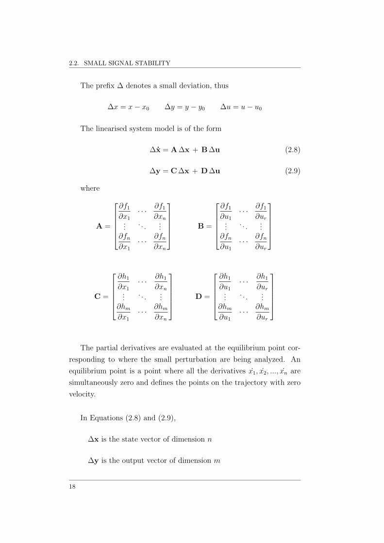
∆x = A ∆x + B ∆u (2.8)
∆y = C ∆x + D ∆u (2.9)
where
A =
∂f1∂x1
· · · ∂f1∂xn
.... . .
...∂fn∂x1
· · · ∂fn∂xn
B =
∂f1∂u1
· · · ∂f1∂ur
.... . .
...∂fn∂u1
· · · ∂fn∂ur
C =
∂h1∂x1
· · · ∂h1∂xn
.... . .
...∂hm∂x1
· · · ∂hm∂xn
D =
∂h1∂u1
· · · ∂h1∂ur
.... . .
...∂hm∂u1
· · · ∂hm∂ur
The partial derivatives are evaluated at the equilibrium point cor-
responding to where the small perturbation are being analyzed. An
equilibrium point is a point where all the derivatives x1, x2, ..., xn are
simultaneously zero and defines the points on the trajectory with zero
velocity.
In Equations (2.8) and (2.9),
∆x is the state vector of dimension n
∆y is the output vector of dimension m
18

CHAPTER 2. POWER SYSTEM STABILITY CONCEPTS
∆u is the input vector of dimension r
A is the state or plant matrix of size nxn
B is the control or input matrix of size nxr
C is the output matrix of size mxn
D is the (feed-forward) matrix which defines the proportion of
inputs appearing directly in the outputs, size mxr
Eigenvalues and eigenvalue properties
Small signal stability analysis studies the properties of the system
((2.8), (2.9)) around (x0, z0, y0) through an eigenvalue analysis of the
state matrix A. Each eigenvalue, denoted by λ, describes one special
dynamic behaviour of the system called a mode which is obtained from
A matrix.
For an operating point to be stable, the real parts of all eigenvalues
of A must lie in the left half-plane of the complex plane (i.e, with neg-
ative real parts). This ensures that oscillations will decay with time
and will return to a steady state following a small disturbance. The
opposite will occur if an eigenvalue has a positive real part. The am-
plitude of the modes will increase exponentially and the power system
will be unstable at that operating point.
If A is real, complex eigenvalue occur in conjugate pairs, and each
pair would correspond to an oscillatory mode. Fig. 2.1 shows the pos-
sible natural modes of a system.
The eigenvalues of A contain essential information about the mode’s
frequencies and their damping after a small disturbance. The real part
component gives the damping and the imaginary component gives the
frequency of oscillation.
19

2.2. SMALL SIGNAL STABILITY
0 50 100 150 200 250 300 350 400 450 5000
0.5
1
1.5
2
2.5x 10
4
s
jw
xx
s
jw
xx
s
jw
x
s
jw
x
x
s
jw
x
x
z1
t
t
z2
z1
z2
z1
z1
z2
0 50 100 150 200 250 300-0.8
-0.6
-0.4
-0.2
0
0.2
0.4
0.6
0.8
1
t
0 100 200 300 400-3000
-2500
-2000
-1500
-1000
-500
0
500
1000
1500
2000
t
0 500 1000 1500 2000 2500 3000-1
-0.8
-0.6
-0.4
-0.2
0
0.2
0.4
0.6
0.8
1
t
z2
x
z2
z1
Eigenvalues
l = s ± jw
Trajectory Time depend characteristic
Figure 2.1: Possible combination of eigenvalues pairs (left). Their trajecto-ries (middle) and time responses (right).
20

CHAPTER 2. POWER SYSTEM STABILITY CONCEPTS
For a complex eigenvalue λi = σi ± jωi, the damping ratio ζ is
defined as:
ζi = − σi√σ2i + ω2
i
(2.10)
with ζ ∈ [−1, 1].
The damping ratio ζ determines the rate of decay of the ampli-
tude of the oscillation. The time constant τ of the amplitude decay is
τ = 1/|σ| [21].
The damping is an important measure of the quality of the system’s
transient response. A poorly damped system oscillates for a relatively
long time following a disturbance, an undesirable characteristic which
ought to be minimized.
Several researchers have addressed the issue of small signal secu-
rity, which is strongly related to the damping of system oscillations
[25, 26, 27, 28]. Minimum admissible dampings have been defined to
be in the range 3 to 5%.
The oscillation frequency f of the ith mode, in Hz, is defined as:
fi =ωi2 π
(2.11)
Mode shape and eigenvectors
The shape of a mode that corresponds to a certain eigenvalue is de-
scribed by its associated right eigenvector, which defines the relative
activity of the system’s dynamic states on each mode.
The eigenvectors are determined regarding the chosen states for the
formulation of the power system model, but it is not a good indicator of
the importance of states to a mode, since eigenvectors are not unique.
The left eigenvector weighs the contribution of the states within a
mode.
21

2.2. SMALL SIGNAL STABILITY
The right eigenvector Φi and the left eigenvector Ψi associated with
the ith eigenvalue λi satisfy
AΦi = λiΦi (2.12)
ΨitA = Ψi
tλi (2.13)
Eigenvalue sensitivity
Differentiating equation (2.12) with respect to akj the element of A in
kth row and jth column yields
∂A
∂akjΦi + A
∂Φi
∂akj=
∂λi∂akj
Φi + λi∂Φi
∂akj
Pre-multiplying by Ψi
Ψi∂A
∂akjΦi + Ψi(A− λiI)
∂Φi
∂akj= Ψi
∂λi∂akj
Φi
and knowing that ΨiΦi = 1 and Ψi(A− λiI) = 0, the above equa-
tion simplifies to
Ψi∂A
∂akjΦi =
∂λi∂akj
Since the only non-zero partial derivatives of A with respect to akj
are equal to 1 (corresponding to element in the kth row and jth column),
∂λi∂akj
= Ψik Φji (2.14)
Therefore the sensitivity of the eigenvalue λi to the element akj of
the state matrix is equal to the product of the left eigenvector element
Ψik and the right eigenvector element Φji [21] .
Participation Factors
Participation factor represents a measure of the contribution of each
dynamic state in a given mode or eigenvalue.
22

CHAPTER 2. POWER SYSTEM STABILITY CONCEPTS
In terms of eigenvectors, the participation factor may be defined
by:
pfki =ΨkiΦik
ΨtiΦi
(2.15)
where Ψki and Φik are the kth entries in the left and right eigenvec-
tors associated with the ith eigenvalue.
The participation matrix Pf , proposed in [29, 30], is defined as:
Pf =[pf1 pf2 ... pfn
](2.16)
with
pfi =
pf1ipf2i
...
pfni
=
Φ1iΨi1
Φ2iΨi2
...
ΦniΨin
(2.17)
By using the scale property of an eigenvector it is possible to choose
a scaling that simplifies the use of participation factors. Thus, by choos-
ing eigenvectors such ΨitΦi = 1, a normalised form of the participation
factor is defined as:
pfni=|Φni| |Ψin|n∑i=1
|Φni| |Ψin|(2.18)
where n is the number of state variables, pfniis the participation
factor of the system. The pfnimagnitude represents a measure of the
relative participation of the nth state variable into mode i, and vice
versa. A further normalization can be done by making the highest of
the participation factors equal to unity. From equation (2.14), it can
be observed that the participation factor pfki is equal to the sensitivity
of the eigenvalue λi to the diagonal element akk of A,
pfki =∂λi∂akk
(2.19)
23
2.2. SMALL SIGNAL STABILITY
In power systems, participation factors can be used as a comple-
mentary measure to the suitability of power system stabilizers (PSS)
placement.
Transfer Function
Although eigenvalue analysis of the system state matrix is carried out
to examine small signal stability of power systems, modal analysis is
very useful when it comes to control design, addressing the open-loop
transfer function and its relationship to the state matrix and its eigen-
properties.
The transfer function has the general form of:
G(s) = KN(s)
D(s)(2.20)
By applying the method used in [21], it can be seen that G(s) may
be written as:
G(s) =n∑i=1
Ri
s− λi(2.21)
where the residues, Ri, in terms of the eigenvectors
Ri = c ΦiΨi b (2.22)
It can be seen that the poles of G(s) are given by the eigenvalues
of A.
2.2.3 Methods for Modal analysis
The eigenvalues of the system state matrix can be computed by solv-
ing the characteristic equation of first and second order systems. For
higher-order systems a method that has been widely used is the QR
transformation method [31, 32].
In this method, a tridiagonal matrix Q is constructed from a set of
orthogonal transformations applied to A matrix. A good description
of the method can be found in [33].
24

CHAPTER 2. POWER SYSTEM STABILITY CONCEPTS
Application of the QR method is confined to small size power sys-
tems with up to approximately 80 generators. Due to computer limita-
tions it has only used in systems containing up to about 800 modes [28].
For larger power systems, special techniques have been developed,
in which partial modal analysis is used. The first algorithm was the
Analysis of Essentially Spontaneous Oscillations in Power Systems (AE-
SOPS), originally presented in [34], which uses the quasi-Newton itera-
tion method to find eigenvalues associated with rotor angle modes close
to initial value set. It is able of handle up to about 2000 states.
Other more efficient methods such as the Inverse Iteration, Gener-
alized Rayleigh Quotient Iteration, Modified Arnoldi [35] and, Simulta-
neous Inverse Iteration [35] have been proposed. All these methods are
based on iterative multiplication of a vector by the system state matrix
A. The Program for Eigenvalue Analysis of Large Systems (PEALS)
combines the AESOPS and the modified Arnoldi method. It is pre-
sented in [36].
On the other hand, Selective Modal Analysis (SMA) focuses on
the relevant eigenvalues in a specific area and therefore, storage and
computer requirements are heavily reduced. This method is described
in [30] and [37].
2.3 Transient Stability Analysis
The so-called transient stability analysis aims to assess the dynamic
response of a power system when subjected to a contingency, such as
line outage or a short circuit of different types: phase-to-ground, phase-
to-phase-to-ground, or three-phase. Although they are commonly as-
sumed to occur in transmission lines, occurrences in buses or trans-
former should also be considered. Of course, as the transient analysis
pertains to stability under large disturbances, the non-linearities of the
25
2.3. TRANSIENT STABILITY ANALYSIS
model have to be taken into account and, hence, linearization of the
power system is deemed as not valid.
In contrast to the small signal stability analysis, the system com-
monly presents a stable pre and post-disturbance equilibrium. The
point in question is whether or not the trajectory of the system follow-
ing the contingency is unstable and reaches a new stable equilibrium
operating point. Caution needs to be exercised though, because al-
though the system may reach a stable operating point from the mathe-
matical vantage, it cannot be considered transiently stable if the mode
of operation is not an acceptable one. From a mathematical viewpoint,
“transient stability implies that an acceptable post-disturbance steady-
state operating condition of the power system is asymptotically stable
and the response to the given disturbance is such that the trajectories
of the operating quantities tend to this operating condition as time in-
crease” [38].
The study’s period of interest may be cover 3 to 5 seconds and per-
haps extended to go up to 10 seconds in some special cases.
With regards to the simulation method some of the most important
techniques that have been used thus far are a) carrying out numerical
integrationof the differential equations that describe the system and ob-
serve the power system response; b) using Lyapunov-based approaches
based on energy functions of the power system; and c) carrying out
probabilistic solutions.
The stability or otherwise of the first solution a), is determined
by the convergence (divergence) of the time domain simulation. The
accuracy of this approach depends only on the numerical integration
method and on the system model. In a complete contingency analysis
this is applied in off-line environments, but for on-line applications
the computational burden of the method is an important issue to be
considered.
26
CHAPTER 2. POWER SYSTEM STABILITY CONCEPTS
The second approach is known as the transient energy function
(TEF), a method in which a stability criterion substitutes the numer-
ical integration. TEF is based on an analytical representation of the
system to determinate the transient kinetic and the potential energy
for the post-contingency system. The energy responsible for the devi-
ation from synchronous operation is quantified by the transient kinetic
energy, whereas the integral of the instantaneous real power mismatch
between electrical and mechanical power at generator buses defines the
potential energy [39].
In the last method, stability is assessed by examining probability
distribution functions resulting from initiating factors such as fault
type, fault location, system conditions, (loading and configuration)
which are probabilistic in nature. This seems to be a tool more suitable
for planning purposes; statistically meaningful results require a large
amount of computation time [40].
2.4 Wind Power Generation Systems
Although many wind turbine designs have been proposed over the
years, the horizontal axis, three-blades, upwind turbines have prevailed
because they have proved to offer an efficient configuration.
Fixed-speed and variable speed are the two types used for wind
energy conversion; fixed- speed operation is generally associated with
smaller turbines whereas variable speed operation is associated with
the largest machines.
2.4.1 Fixed-speed Wind Turbines
The fixed-speed or constant speed generator is based on a directly
coupled conventional squirrel-cage induction generator whose slip, and
hence the rotor speed, vary depending on the amount of generated
power.
27

2.4. WIND POWER GENERATION SYSTEMS
However, the rotor speed variation is generally 1 or 2 percent [5, 41].
The configuration of a FRC is illustrated in Fig. 2.2.
Squirrel-cage induction generators always consume reactive power
and therefore, the factor power correction is provided by capacitors at
each wind turbine. The power control is done by stall and pitch con-
trol which allow reducing the aerodynamic efficiency of the rotor. The
first one (stall) corresponding to the design of the rotor blades reduces
the efficiency of wind speed above nominal value. With pitch control
the efficiency is reduced by turning the blades out of the wind using
hydraulic mechanisms or electric motors [41].
Both, advantages and drawbacks of this generation system can be
summarizes as follows [41, 42]:
• This is a relatively simple generation system and less expensive.
• FSIG-based wind farms can contribute to network damping but
their ability to survive network faults is poor.
• The fluctuations of the drive train torque produced by fluctua-
tions in wind speed could lead to high structural loads due to the
lack of capability to vary the rotor speed. This requires a more
mechanically robust turbine.
Gearbox
SCIG
Grid
Wind
Capacitor bank
Figure 2.2: Configuration of a fixed-speed wind turbine.
28
CHAPTER 2. POWER SYSTEM STABILITY CONCEPTS
2.4.2 Variable-speed Wind Turbines
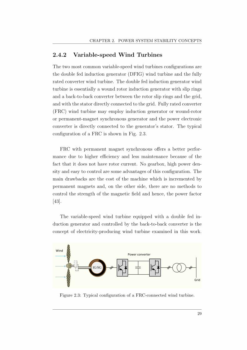
The two most common variable-speed wind turbines configurations are
the double fed induction generator (DFIG) wind turbine and the fully
rated converter wind turbine. The double fed induction generator wind
turbine is essentially a wound rotor induction generator with slip rings
and a back-to-back converter between the rotor slip rings and the grid,
and with the stator directly connected to the grid. Fully rated converter
(FRC) wind turbine may employ induction generator or wound-rotor
or permanent-magnet synchronous generator and the power electronic
converter is directly connected to the generator’s stator. The typical
configuration of a FRC is shown in Fig. 2.3.
FRC with permanent magnet synchronous offers a better perfor-
mance due to higher efficiency and less maintenance because of the
fact that it does not have rotor current. No gearbox, high power den-
sity and easy to control are some advantages of this configuration. The
main drawbacks are the cost of the machine which is incremented by
permanent magnets and, on the other side, there are no methods to
control the strength of the magnetic field and hence, the power factor
[43].
The variable-speed wind turbine equipped with a double fed in-
duction generator and controlled by the back-to-back converter is the
concept of electricity-producing wind turbine examined in this work.
IG/SG
Grid
WindPower converter
Figure 2.3: Typical configuration of a FRC-connected wind turbine.
29
2.4. WIND POWER GENERATION SYSTEMS
Grid
DFIG
Gearbox
Wind
Power converter
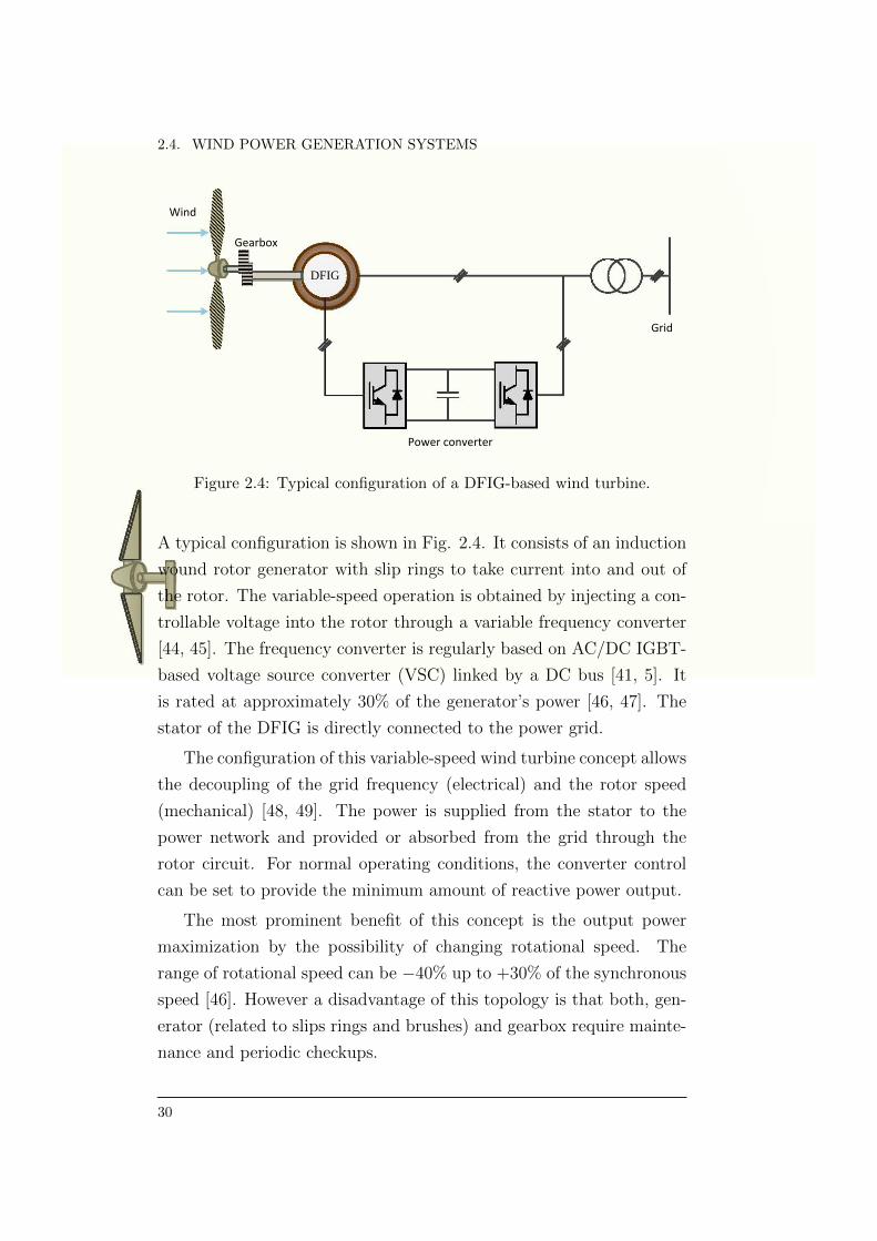
Figure 2.4: Typical configuration of a DFIG-based wind turbine.
A typical configuration is shown in Fig. 2.4. It consists of an induction
wound rotor generator with slip rings to take current into and out of
the rotor. The variable-speed operation is obtained by injecting a con-
trollable voltage into the rotor through a variable frequency converter
[44, 45]. The frequency converter is regularly based on AC/DC IGBT-
based voltage source converter (VSC) linked by a DC bus [41, 5]. It
is rated at approximately 30% of the generator’s power [46, 47]. The
stator of the DFIG is directly connected to the power grid.
The configuration of this variable-speed wind turbine concept allows
the decoupling of the grid frequency (electrical) and the rotor speed
(mechanical) [48, 49]. The power is supplied from the stator to the
power network and provided or absorbed from the grid through the
rotor circuit. For normal operating conditions, the converter control
can be set to provide the minimum amount of reactive power output.
The most prominent benefit of this concept is the output power
maximization by the possibility of changing rotational speed. The
range of rotational speed can be −40% up to +30% of the synchronous
speed [46]. However a disadvantage of this topology is that both, gen-
erator (related to slips rings and brushes) and gearbox require mainte-
nance and periodic checkups.
30
I~ ItO

CHAPTER 2. POWER SYSTEM STABILITY CONCEPTS
2.5 Variable-speed Wind Turbine Systems
Integrated in Power Systems
Technical aspects, such as the use of converter utility interfaces, the in-
herent uncontrollability of the wind, and the existence of machines of
smaller size make a distinction between wind power system generation
and conventional synchronous generation systems and their interac-
tion with power networks. Impacts both, local (power flows, busbar
voltages, protection schemes, power quality) and system-wide (system
dynamics, system stability, reactive power, voltage and frequency sup-
port) affect the system’s behaviour either in the vicinity or as a whole.
As described above, fixed-speed and variable-speed wind turbines
are the two main categories used at wind power systems. However
thanks to the development of power electronics and their cost reduc-
tion, the variable-speed wind technology becomes a competitive can-
didate for the wind energy system operation. This is the addressed
technology in this thesis.
Variable-speed turbines can affect their terminal voltage by mod-
ifying the exchange of reactive power. The use of power electronic
converters in this kind of wind turbine is an important subject. Re-
garding power quality the attention is focused on harmonic distortion.
In case of faults, the wind turbine may be disconnected from the grid
by intervention of the converter control system: in FRC wind turbine
by blocking the turn-on pulses for the converter; in DFIG-based wind
turbines, in case of too high rotor voltages, the rotor windings are
short-circuited by a crowbar protection system.
This is an important issue concerning the power system stability.
The consequences of disconnecting the wind turbines in a high wind
penetration scenario, i.e., above 10% [46], can lead to voltage drops
which degrade the power generation performance. Thus, nowadays,
31

2.5. VARIABLE-SPEED WIND TURBINE SYSTEMS INTEGRATED INPOWER SYSTEMS
new technical requirements for the reliable operation of large wind en-
ergy systems interconnected to the power grid are imposed by grid
codes [50, 51].
Dynamic advantages of the variable-speed DFIG wind turbines in-
clude enhancement of machine stability margin and damping of system
oscillations. However, under transient conditions, as the ones me above
mentioned, the generator works as a traditional squirrel cage induction
generator due to the fact that the protection scheme acts to short cir-
cuit the rotor.
Comparative studies between this concept with synchronous gen-
erators (SG) and squirrel cage induction generators (SCIG) have been
considered to analyze how the dynamic behaviour of the DFIG itself
affects stability of the power system. The studies have been carried
out by considering both frequency domain and time domain approach.
An analysis using a frequency-domain approach based on eigenvalue
analysis has been performed to examine the impact of the DFIG-based
wind turbine on the low-frequency oscillatory modes of the synchronous
machines [52, 53, 54, 55, 56]. The time domain approach has been ex-
tensively used throughout the literature to investigate voltage dynamics
of power systems subject to large disturbances [57, 58, 59, 60, 61].
The decoupled controllability of the d-axis and q-axis component
of the DFIG rotor voltage vector confers greater flexibility. It is a sig-
nificant difference between DFIG and both, SG and SCIG. In case of
SG, developed excitation systems use additional control such as power
system stabilizer to control the field voltage, to damp system oscilla-
tions, and, in general, to enhance the whole system dynamic perfor-
mance. In case of SCIG, additional components, e.g. power electronic-
based compensator, are inherent associated with any dynamic control
[62, 63, 64, 65].
32

CHAPTER 2. POWER SYSTEM STABILITY CONCEPTS
Otherwise, in recent years a growing interest in studying the DFIG
frequency support is justified because the DFIG does not contribute to
any inertial response to frequency events (as a fixed-speed wind turbine
with induction machine does) [66]. Although it has not been studied
extensively, some papers deal with the impact of DFIG frequency re-
sponse [19, 67, 68], but because of their assumptions, there are some
discrepancies between the pointed out conclusions. None of these pa-
pers discusses the limiting factors of DFIG frequency support.
The interest on this topic also increases along with the risk of oc-
currence of frequency variations because of interactions between large
active power variations, an installed high wind power capacity, and the
existence of frequency controllers in the conventional power stations.
In order to quantify the extra active power support provided from
a variable-speed wind turbine at a certain wind speed, it is calculated
the amount of energy that can be extracted from the wind turbine with
along the extra energy from the stored rotational energy in the turbine-
generator [69]. As expected, the capability of providing an extra active
power support of the wind turbine is reduced at high wind speed con-
ditions (above medium wind speed) and hence, the dimensions of the
turbine mechanical design and the power rating of the generator side
converter need to be suitably adjusted. In [70], a variable proportional
controller to facilitate a temporary extra wind turbine active power
support in high wind speed conditions is proposed, in which a maxi-
mum delivery of 5% and 10% extra active power was reported.
Implementation of primary frequency regulation in wind turbines
can be found in [20, 71, 72, 73, 74, 75].
Acknowledging the control capabilities of the DFIG, the authors in
[55], brought forward a power system stabilizer for a wind turbine em-
ploying a DFIG and showed that this PSS could significantly influence
the contribution of a DFIG-based wind farm to network damping. The
power system stabilizer was designed to operate with a flux magnitude
33

2.5. VARIABLE-SPEED WIND TURBINE SYSTEMS INTEGRATED INPOWER SYSTEMS
and an angle controller (FMAC) scheme, by which the terminal voltage
and the stator power output can be controlled via the magnitude of the
rotor flux vector and its angular position.
The control strategies usually adopted are those one based on in-
ertial control, using the kinetic energy stored in the rotating masses
and the proportional control implemented in conventional units. The
possibility of releasing kinetic energy from a DFIG-based wind turbine
system by adding an extra control loop, sensitive to the network fre-
quency, has also been applied in works as [76, 19] and compared to
fixed-speed wind turbines [42, 67].
Considering the published results it can be concluded that variable
speed DFIG farms with frequency control managed to increase the
eigenvalues damping, improving as well the dynamic response of the
frequency. This improvement is more significant in DFIG-based wind
farms with frequency control than in the fixed-speed SCIG.
34

Chapter 3
Variable-Speed Wind Power
Generation Systems
Some basic considerations concerning the performance of wind turbines
in electrical power systems are presented in this chapter. To this end,
an introduction to aerodynamic aspects of wind turbines is presented,
followed by a brief overview of the concept of modelling, simulation
aspects, and the main elements of a variable-speed wind turbine model
in connection with the type of studies addressed in this work.
3.1 Introduction
Computer simulations of complex systems, as it is the case of wind
turbines, make possible to investigate a wide range of properties of key
technology aspects such as design, construction and applications.
It is fair to say that investigation has its own requirements concern-
ing its necessary level of modelling detail and the model data require-
ments all of which need to be agreed on before simulation can start.
This is strongly related to the accuracy and reliability of the obtained
results.
35
3.2. WIND SPEED
In this way, an overview of the wind turbine generation system is
first presented aimed at having a good understanding of the technology
with a view to assess the relevance of each one of its components within
the scope of this thesis.
3.2 Wind Speed
The modelling of power fluctuations of wind farms in continuous op-
eration may be a key requirement to obtain realistic results in most
studies. Wind speed is one of the most difficult variables to predict
in order to estimate the wind farms energy production and to get an
acceptable analysis of its behaviour when connected to the electrical
network.
Theoretical estimations can be collected by means of statistical data
related to wind variations at a particular location, although these are
better suited for planning stage in terms cost, electricity output per unit
and area. To ensure that all design limits are satisfied, the performance
evaluation of wind power generation system schemes has be considered
in the full range of wind speed variations. Stochastic and deterministic
effects (caused by turbulences, the tower shadow, etc.) have been taken
into account by means of various wind functions.
For power output of a wind turbine the long-term variations of the
mean wind velocity are of great importance while short-term fluctua-
tions determine the fatigue loading on the wind turbine structure.
The wind, in time, can be regarded as having a quasi-static mean
speed which fluctuations superimposed on the average value. Random
variations of the instantaneous speed from the mean wind speed in
periods below 10 minutes are considered as termed turbulences [77].
Turbulences are caused by the airflow over the earth’s surface and are
influenced by orography characteristics, soil surfaces or by the presence
of obstacles such as buildings.
36

CHAPTER 3. VARIABLE-SPEED WIND POWER GENERATION SYSTEMS
The mean wind speed vw (generally over a period of ten minutes),
ignoring short-term fluctuations, is determined by the level of wind
speed. Thus, the instantaneous wind speed can be expressed as a
function of a steady mean wind speed vw(y, z) and a field of turbulence
vT (y, z, t) corresponding to the superimposed fluctuating part of the
wind speed
v(y, z, t) = vw(y, z) + vT (y, z, t) (3.1)
A more common measure of the wind variability is the turbulence in-
tensity index, which is defined as the relation of the standard wind
speed deviation to the mean wind speed
IvT =σwvw
(3.2)
This index can be up to 20% over forest or urban areas [78].
Other kind of wind fluctuations denominated gusts, also exist and
may vary from a few to several tens of seconds. The average wind
speed is often modelled by a Weibull distribution function whose den-
sity function is given by
p(v) =(ab
)(vb
)a−1exp
[−(vb
)a](3.3)
where p(v) is the probability related to wind speed v, b is the scale
factor, and a is the form factor.
The so-called Rayleigh distribution is a special case of Weibull dis-
tribution, in which the a parameter is assumed to be equal to 2 [79, 80].
Both distributions fit quite well to most wind histograms and b and a
can be determined by applying common estimation methods such as
the standard deviation method (SD), the maximum likelihood method
(MLM), and the least squares method (LSM) [81]. Wind speed in-
creases with height because of friction at the earth surface [82]. The
increase rate of wind speed is given by
v(z) = v0
(z
z0
)α(3.4)
37

3.3. MECHANICAL SYSTEM OF A WIND TURBINE
where v is the predicted wind speed at height z and v0 is the wind speed
at height z0. This results in a significant increase in power greater
heights. At the same time, α is an empirical parameter of the wind
shear and it can take a value of either 1/7 (during the day) and 1/5
(during the night) [83]. For more specialised information on wind speed
in wind turbines the following references [84, 85], are particularly useful.
3.3 Mechanical System of a Wind Tur-
bine
The wind mechanical turbine model represents essentially the shaft
dynamics of the wind turbine and its control system. The main me-
chanical turbine components are the blades, hub, shafts and depending
on the wind turbine technology, the gearbox.
In this section, the energy conversion process is addressed to explain
the role that the drive train elements play in the wind power extraction
process. Afterwards the shaft system model is presented.
3.3.1 Principles of wind energy conversion
Elementary momentum theory
The elementary “momentum theory” provides a common physical basis
for the understanding and operation of wind energy conversion. The
analysis considers a control volume bordered by a surface of a stream
tube and two cross-sections of the stream tube, as shown in Fig 3.1.
An uniform ‘actuator disc’ represents the turbine.
This theory states that the kinetic energy of an air mass m, moving
at a velocity v can be expressed as
E =1
2mv2 (3.5)
38

CHAPTER 3. VARIABLE-SPEED WIND POWER GENERATION SYSTEMS
Pmech
Actuator
disc
v2
axial
Stream-tube
v1 v'
Figure 3.1: Flow model of momentum theory
The volume V flowing through a certain cross-sectional area A,
through which the air passes at velocity v, is
V = vA (3.6)
and the mass flow with air density ρ is
m = ρvA (3.7)
The energy passing through the cross-section A per second, which
has been produced by the kinetic energy of the moving air and the
mass flow, is identical to the power P
P =1
2ρv3A (3.8)
The mass flow through the stream-tube must remain unchanged
everywhere. Therefore, the flow velocity increases due to its narrow
cross-sectional area.
The power difference of the air flow upstream and downstream of
the converter yields the mechanical energy that has been previously
39

3.3. MECHANICAL SYSTEM OF A WIND TURBINE
extracted from the airflow
P =1
2ρA1v
31 =
1
2ρA2v
32 =
1
2m(v21 − v22) (3.9)
Downstream v1 is the wind velocity before it gets to the converter,
whereas v2 is the flow velocity behind the converter. In theory, the
power would reach its maximum level when the downstream velocity is
zero. However, the wind speed cannot be reduced to zero in practice.
This equation is of great importance since it reveals that the power in-
creases with the cube of wind speed and only linearly with air density
and swept area.
Conservation of momentum provides the relationship between the
converter thrust, T , and the rate of change of momentum of the airflow,
T = m(v1 − v2) (3.10)
The net force on the control volume must be equal and opposite to
the converter thrust, which is an equal force exerted by the converter
on the air stream. In this sense the required power is
P = Fv′= m(v1 − v2)v
′(3.11)
Thus the mechanical power extracted from the air stream can be
deduced from both, the power difference between the upstream and
downstream of the converter and the thrust and the flow velocity. By
equating (3.9) and (3.11)
1
2m(v21 − v22) = m(v1 − v2)v
′(3.12)
The power coefficient Cp is defined as the ratio of the wind power
and the mechanical power output of the converter,
Cp =Pwind turbine
Pair
(3.13)
40

CHAPTER 3. VARIABLE-SPEED WIND POWER GENERATION SYSTEMS
A theoretical ideal maximum coefficient Cp, which was derived by
Betz [78], is Cp = 1627
= 0.593 1
The dependency of the power coefficient on such a relationship,
when looked at from the energy vantage, is what it is termed tip-speed
ratio λ, which is determined by the ratio of the rotor blade’s tangential
velocity in the undisturbed axial airflow and the wind speed. It is
commonly referenced to the tangential velocity of the rotor blade tip,
uT .
λ =uTvw
=tangential velocity of the rotor blade tip
wind speed(3.14)
or
λ =ωR
v(3.15)
where
ω = rotational speed of rotor
R = radius to tip of rotor
v = upwind free wind speed, m s−1
The tip-speed ratio λ, and the power coefficient Cp are dimension-
less and are well suited to characterize the performance of any size of
wind turbine rotor, as it will be described later in the chapter.
Blade element momentum
The physical framework from which the analysis of conversion of kinetic
energy to mechanical energy is developed, should not be separated from
the actual capabilities of the energy converter. Under real conditions,
the power output depends on the aerodynamic forces that have been
employed to produce it.
1It is frequently called the Betz factor or Betz limit. Modern wind turbines,operate close to the power coefficient limit, with Cp up to 0.5 and are thereforeoptimized because of this.
41
3.3. MECHANICAL SYSTEM OF A WIND TURBINE
Such forces, expressed as a function of the local aerodynamic lift
and drag coefficients, can be derived by using the blade element theory,
which divides the rotor blade into a number of elements. Both, the
velocity component in the span-wise direction and three-dimensional
effects are ignored.
Fig. 3.2 shows all the forces and velocities relative to the blade
chord line at radius r. The blade elements are formed by the local ro-
tor blade chord and the radial extension of the element δr. The incident
resultant velocity, vr, is obtained from the combination of the axial flow
velocity in the rotor plane and the tangential speed at the radius of the
blade cross-section. The angle of attack is an aerodynamic parameter
formed from vr in the cross-sectional plane of the blade. The blade
pitch angle is a geometrical parameter (design parameter) referring to
the plane of rotation.
The lift force, L, is perpendicular to the flow direction, and the
drag force, D, is parallel to the flow direction. These forces are defined
by following relations
L =1
2ρairv
2r cCL (3.16)
D =1
2ρairv
2r cCD (3.17)
where c is the chord of the blade section and CL and CD are the
lift and the drag coefficients, respectively, which can be determined by
using the airfoil data catalogues.
The normal and tangential forces, FN and FT , acting on the blade
sections are
FN = L cosφ+D sinφ (3.18)
FT = L sinφ+D cosφ (3.19)
with φ being the angle between the relative velocity and the rotor
plane,
φ = arctan(vaxialrω
)42

CHAPTER 3. VARIABLE-SPEED WIND POWER GENERATION SYSTEMS
dr
r
b : blade pitch angle
a : angle of attack
a
b
vrxi lva a
tangential r fo ce
agdr
wind
wspeed v
i c o d re ti n ofa rot tion
wr.
chord
a usxial force (thr t)
lift e rr sultant ai force
Figure 3.2: Flow velocities and aerodynamics forces at a blade element
43
- ......... ..... ....
/ .... / ,
/ \
1'/ /;:: • :~~ ••• '.\."""'\\' \\ (( ,,1 : \ ; ........ !.J .... ) ~~ -' /
\ \ / ....... ::::::::::...... / I \
.... / .... /
........... _-- -
----

3.3. MECHANICAL SYSTEM OF A WIND TURBINE
On this basis, the exerted forces on the blade element moving though
the stream tube-strip can be calculated. Assuming that there is no
aerodynamic interference between the strips, the forces on the blade
elements distributed over the blade length can be added, and hence
the aerodynamic force distribution over the blade length is obtained.
The rotor torque is obtained by the integration of the tangential
force distribution and the power coefficient Cp or the rotor power with
the rotor speed.
The rotor thrust is obtained from the axial force distribution. Thus,
both the rotor performance and the aerodynamic loading for a given
rotor geometry can be determined by applying the blade theory.
Further details on theoretical modelling concepts are available in
the literature [78, 86, 87].
3.3.2 Wind turbine rotor performance and model
for power system studies
The power, torque and rotor thrust are the three main indicators used
to assess the performance of a wind turbine, depending on how these
vary with wind speed.
The amount of energy taken from the wind and the gearbox size
are defined by the power and the developed torque, respectively. The
wind turbine tower design is strongly linked to the rotor thrust.
For power system studies the wind turbine is represented by a non-
linear wind power model relating power output Pt to wind speed vw and
power coefficient Cp. Since the interest is mainly focused on the input
torque, the complex airflow dynamics and their associated mechanical
vibrations and deformations are ignored.
44

CHAPTER 3. VARIABLE-SPEED WIND POWER GENERATION SYSTEMS
The available shaft power Pt is calculated as, [5]
Pt =1
2ρair v
3w AwtCp (λ, β) (3.20)
where ρair is the mass density of air, Awt is the wind turbine rotor
swept area, the power coefficient Cp, is a function of the tip speed ratio
λtip and the pitch angle β.
Fig. 3.3 illustrates a power coefficient curve with the pitch angle, β
as parameter. The power coefficient is maximum for a unique tip-speed
ratio. For a fixed-speed wind turbine, operation at maximum power
coefficient corresponds to a particular wind speed; however in variable-
speed wind turbines it is possible to cover a wide range of wind speeds.
Cp− λ curves are obtained from field measurements and are gener-
ally provided by manufacturers. Numerical approximations have been
used to obtain the Cp−λ curves for academic purposes. Using a generic
equation developed in reference [49], Cp can be calculated as
Cp = c1
(c2λi− c3β − c4βc5 − c6
)exp−c7λi
+ c10λ (3.21)
0 2 4 6 8 10-0.1
0
0.1
0.2
0.3
0.4
Tip-speed ratio tip
Pow
er c
oeffi
cien
t C
p
0º
25º
15º
1º
10º
5º
Figure 3.3: Power Coefficient as a function of tip speed ratio and the pitchangle.
45

3.3. MECHANICAL SYSTEM OF A WIND TURBINE
where
λ−1i =
[(1
λ+ c8 β
)−(
c9β3 + 1
)]−1The Cp parameters ci, are given in Table 3.1.
A straightforward and convenient way to obtain the dynamic per-
formance relating to the operating point is by means of power and
torque coefficients curves resulting from the theoretical analysis men-
tioned above.
Power curves of wind turbines give the steady-state relationship
between the net electrical power output and the wind speed at hub
height. These are normally given by the turbine manufacturer.
Fig. 3.4 shows an example of a typical power curve for a wind
turbine.
Table 3.1: Approximation of power curve for a variable-speedwind turbine
c1 c2 c3 c4 c5 c6 c7 c8 c9 c100.73 151 0.58 0.002 2.14 13.2 18.4 -0.02 -0.003 0
Wind speed (m/s)
Ele
ctric
al p
ower
(
MW
)
vw
Pratedvw,rated
vw,co
vw,ci
Figure 3.4: Typical Power curve for a wind turbine
46
CHAPTER 3. VARIABLE-SPEED WIND POWER GENERATION SYSTEMS
The points corresponding to cut-in wind speed, vw,ci, and rated wind
speed, vw,rated, represent the wind speed value at which the machine
will deliver the minimum useful power and the rated power, Prated,
respectively. Due to safety restrictions, the delivery electrical power is
limited at a maximum wind speed, termed cut-out wind speed, vw,co.
The cut-in and the cut-out wind speed are given by the wind designer.
All wind velocities are measured at hub height.
Approximated values for an average annual wind speed of 8 m/s are
[5]:
• cut-in wind speed: 5m s−1
• rated wind speed: 12− 14m s−1
• cut-in wind speed: 25m s−1
In small network disturbance studies a simple turbine model with
constant input power or torque (constant wind speed, rotor speed and
pitch angle) can be used, since the variation in rotor speed, and hence
pitch angle are small.
3.3.3 Shaft system
The shaft system represents the coupling between mechanical and elec-
trical parameters of a wind turbine. For small-signal stability studies
of wind turbines with DFIG’s, a multi-mass drive train must be con-
sidered.
A complete shaft system of a turbine-generator unit can be modelled
as three masses connected by two shafts, as shown in Fig. 3.5. It
consists of turbine, low-speed shaft, gearbox, high-speed shaft, and
generator.
High turbine inertia and low stiffness between the turbine and gen-
erator rotor are distinctive characteristics of wind turbines in contrast
with conventional steam and hydro turbines [88]. Low mechanical shaft
stiffness, viewed from the high-speed shaft, is a result of the gearbox.
47

3.3. MECHANICAL SYSTEM OF A WIND TURBINE
A simplified two-mass model, shown in Fig 3.6, can be obtained
by comparing the shaft stiffness and the masses of the same speed
reference. If k∗LS = kLS/n2gb is the low-speed shaft stiffness referred to
the high-speed side, the high-speed side can be considered rigid respect
to the low-speed shaft, since the gear ratio for machines rated between
300 kW and 2000 kW (with higher rotational speeds between 48 and
17 r.p.m.) is between about 1:31 and 1:88 [86].
Thus, one of the masses is related to the wind turbine (low-speed
shaft) representing the lumped-mass of hub and blades, while the sec-
ond mass represents the equivalent shaft, the high-speed shaft, in which
gearbox and generator inertia are lumped together. The shaft stiffness
in Fig 3.6 is represented by ksh.
turbine
low speed shaft high speed
shaftTm
Te
gearbox generator
Figure 3.5: Three-mass model of drive train
turbine
Tm Te
generator +gearbox
ksh
Figure 3.6: Two-mass model of drive train
48
CHAPTER 3. VARIABLE-SPEED WIND POWER GENERATION SYSTEMS
The two-mass approach is recommended for power system stability
studies because the flexibility (or softness) of the shafts are correctly
represented [89]. It should be emphasised that the gearbox of the wind
turbine represents a low mechanical stiffness, ksh, hence, the two-mass
model is used to preserve correctly the drive train dynamics [90].
The resonance frequency of the low speed shaft is in the range be-
tween 1 and 2 Hz for multi-megawatt wind turbine generators, and
therefore within the frequency band of interest (0.1-10 Hz). The res-
onance frequencies of the gearbox and the high speed shaft are above
this band, hence, these are considered to be infinitely stiff [41].
Moreover, the modes associated with the blades and the hubs are
either well damped or their frequencies are out of the range of interest
[90].
The dynamics equations for the shaft system can be obtained from
Newton’s equations of motion for each mass,
J∗tdω∗tdt
= (T ∗t − Tsh) (3.22)
Jgdωgdt
= (Tsh − Te) (3.23)
dθωtdt
= ωeleB (ω∗t − ωg) (3.24)
with shaft mechanical torque given by:
Tsh = ksh θωt + cdθωtdt
(3.25)
where Jt and Jg are the inertia of the turbine and generator; ωt and
ωR are the turbine and generator speed; Tt and Tg are the torques of
the turbine and generator; ωωt is the shaft torsional angle; and ksh and
c are the equivalent shaft stiffness and damping coefficient. All turbine
variables (angular speed and torque) are referred to the generator side
of the gearbox and are denoted by a superscripted asterisk.
49
3.3. MECHANICAL SYSTEM OF A WIND TURBINE
In power systems it is helpful to normalize all variables and parame-
ters using per unit notation, in order to make all variables dimensionless
and simplify the computation and the system analysis. For that, ap-
propriate reference bases should be chosen, and thus the per unit value
is given by the ratio between the actual value and the base value,
per unit value =actual value
base value(3.26)
The following base speed and base torque are defined to express the
drive train system in per unit values
ωtB =ωRBngb
(3.27)
TtB = TeB ngb (3.28)
where ωRB = ωelB/npp is the base speed of the generator with ωelB
the electrical speed equal to 2πf , and npp the generator’s pole-pair
number, TeB = Prated/ωRB is the base of the generator electrical torque
and, ngb is the gearbox ratio.
With the turbine speed inertia and torque referred to the high-speed
shaft by ω∗t = ngbωt, J∗t = Jt/n
2gb and T ∗t = Tt/ngb, respectively, and
the turbine bases (ωtB, TtB), equation (3.22) in per unit can be written
asJtn2gb
ωRBωtpudt
= TeB(Ttpu − Tshpu) (3.29)
and together with the inertia constant of the turbine (in seconds),
Ht =1
2
Jt ωRBn2gb TeB
(3.30)
yields to the turbine speed equation,
dωtpudt
=1
2Ht
(Ttpu − Tshpu) (3.31)
50

CHAPTER 3. VARIABLE-SPEED WIND POWER GENERATION SYSTEMS
Similarly, the rotor generator speed equation ((3.23)) in per unit
form is obtaineddωgpudt
=1
2Hg
(Tshpu − Tepu) (3.32)
where the electromagnetic torque, Te, in per unit, as presented in
next section, is calculated as
Te = iSd ΨSq − iSq ΨSd (3.33)
The shaft torque from (3.25) can be expressed in per unit by apply-
ing the per unit definition (equation (3.26)) with the stiffness base
as kB = TeB/(1 el.rad) and the base damping coefficient as cB =
TeB/(1 el.rad/1 s)
Tshpu = kshpu θωt + cpudθωtdt
(3.34)
The equation (3.24) for the equivalent twist angle is expressed in
actual units (radians). The equations for the drive train system are
summarized as below. The system model in this document is assumed
to be expressed in per unit notation, therefore the subscript ‘pu’ and
superscript ‘∗’ are omitted, from now on,
dωtdt
=1
2Ht
(Tt − Tsh) (3.35)
dωgdt
=1
2Hg
(Tsh − Te) (3.36)
Tsh = ksh θωt + cdθωtdt
(3.37)
dθωtdt
= ωeleB (ωt − ωg) (3.38)
3.4 Electrical System of a Wind Turbine
Equipped with DFIG
Along with the mechanical drive train, the electrical system is a fun-
damental part of a wind turbine. The electrical system comprises the
51

3.4. ELECTRICAL SYSTEM OF A WIND TURBINE EQUIPPED WITHDFIG
components necessary to convert the mechanical energy into electric
power, including electrical auxiliaries and control systems.
The electrical generator is the central component for the mechani-
cal/electrical energy conversion process in a wind turbine. Nowadays,
wind turbines equipped with double fed induction generators are the
most widely used variable speed wind turbine technology for large wind
turbines (above 1 MW). It consists essentially of a wound rotor induc-
tion generator with slip rings and a back-to-back converter between the
rotor slip rings and the grid, and with the stator directly connected to
the grid. A typical configuration is shown in Fig. 2.4.
The main features of this generator are:
• The range of rotational speed can be −40% up to +30% of the
synchronous speed [46].
• The frequency converter is rated at approximately 30% of the
rated generator power [46, 47].
• The grid frequency (electrical) and the rotor speed (mechanical)
are decoupled [48, 49].
• The power is supplied from the stator to the power network and
provided or absorbed from the grid through the rotor circuit.
Likewise, the controllability of the electrical system is an important
aspect linked to the energy quality of the power system and plays an
important role to ensure its security and stability.
3.4.1 Generator Model
The induction generator comprises three-phase windings in the stator
Sa , Sb, Sc and three-phase windings in the rotor Ra , Rb
, Rc distributed
120 as shown Fig. 3.7.
52
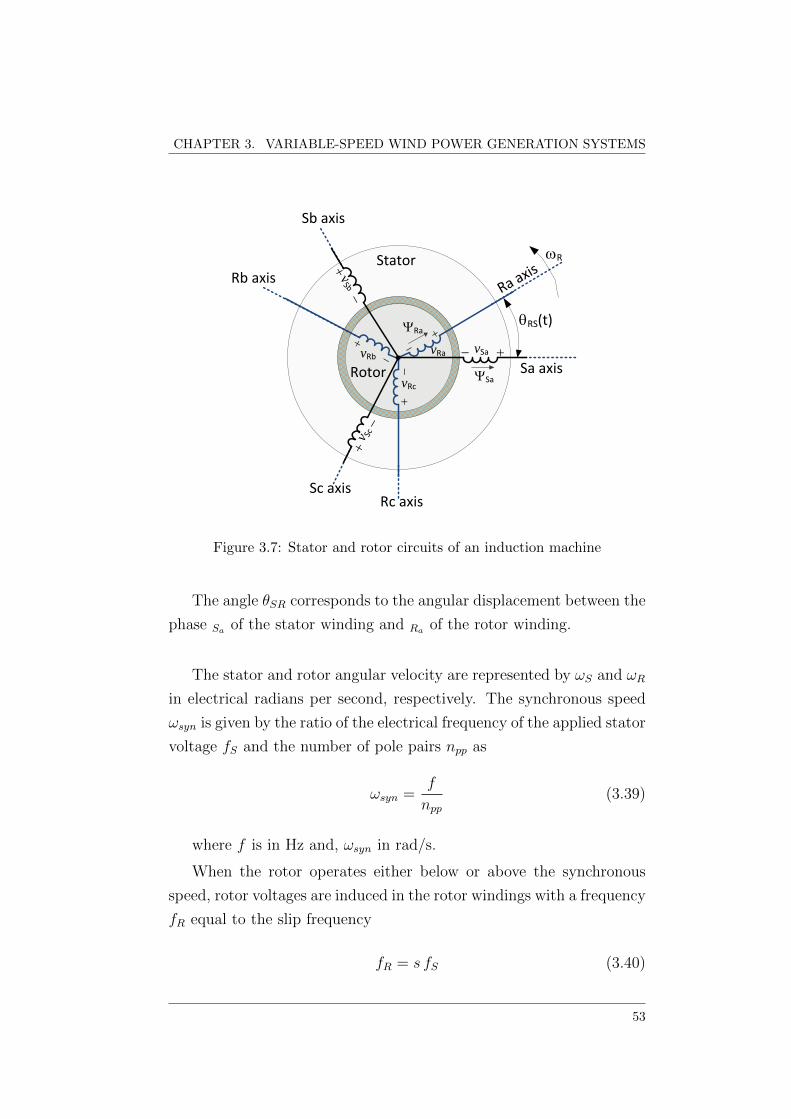
CHAPTER 3. VARIABLE-SPEED WIND POWER GENERATION SYSTEMS
Ra axiswR
Sa axis
Sb axis
Rb axis
Rc axisSc axis
Rotor
Stator
qRS(t)
vRa-
+
vSa- +
YSa
+ -
YRa
vRb
vRc-
+
-
+
+
-
vSb
v Sc
Figure 3.7: Stator and rotor circuits of an induction machine
The angle θSR corresponds to the angular displacement between the
phase Sa of the stator winding and Ra of the rotor winding.
The stator and rotor angular velocity are represented by ωS and ωR
in electrical radians per second, respectively. The synchronous speed
ωsyn is given by the ratio of the electrical frequency of the applied stator
voltage fS and the number of pole pairs npp as
ωsyn =f
npp(3.39)
where f is in Hz and, ωsyn in rad/s.
When the rotor operates either below or above the synchronous
speed, rotor voltages are induced in the rotor windings with a frequency
fR equal to the slip frequency
fR = s fS (3.40)
53

3.4. ELECTRICAL SYSTEM OF A WIND TURBINE EQUIPPED WITHDFIG
where the slip s is given by
s =ωsyn − ωRωsyn
(3.41)
Stable state performance
The equivalent circuit of at double fed induction generator is shown in
Fig. 3.8. In this, V S and IS represent the phase stator voltage and
current, V R and IR the rotor voltage and current, RS and RR the sta-
tor and rotor resistances, Lsl and Lrl are the stator and rotor leakage
inductances and Lo the magnetizing inductance.
From Fig. 3.8 stator and rotor voltage (referred to the stator) are
expressed as
V S = −RS IS + jωS Lsl IS + jωS Lo (IS + IR) (3.42)
V R
s= −RR
sIR + jωS Lrl IR + jωS Lo (IS + IR) (3.43)
The electromechanical torque is given by
Te = 3|IR|2RRnppsωS− 3< [V R I
∗R]nppsωS
(3.44)
Then, the torque is slip dependent.
RS Lsl Lrl
Lo
IRIS
VRVS
+ +
_ _
RR
s
s
Figure 3.8: Steady-state equivalent circuit of the DFIG
54

CHAPTER 3. VARIABLE-SPEED WIND POWER GENERATION SYSTEMS
−1 −0.8 −0.6 −0.4 −0.2 0 0.2 0.4 0.6 0.8 1−3
−2
−1
0
1
2
3
Slip (pu)
Tor
que
(pu
)
Pull−out torque
Motoring operation
Generating operation
Figure 3.9: Typical torque-slip characteristic of an induction machine
Fig. 3.9 illustrates the relationship between torque and slip. When
rotor operates below the synchronous speed (i.e., slip increases) the
machine operates in motoring mode; if rotor speed is greater than
synchronous speed (negative slip) the machine operates in generating
mode.
Dynamic analysis
Depending on stator and rotor windings, the voltage dynamics of the
machine can be described by
vSa(t) = −RS iSa(t)− dΨSa(t)
dt(3.45)
vSb(t) = −RS iSb
(t)− dΨSb(t)
dt(3.46)
vSc(t) = −RS iSc(t)−dΨSc(t)
dt(3.47)
vRa(t) = −RR iRa(t)− dΨRa(t)
dt(3.48)
vRb(t) = −RR iRb
(t)− dΨRb(t)
dt(3.49)
vRc(t) = −RR iRc(t)−dΨRc(t)
dt(3.50)
55
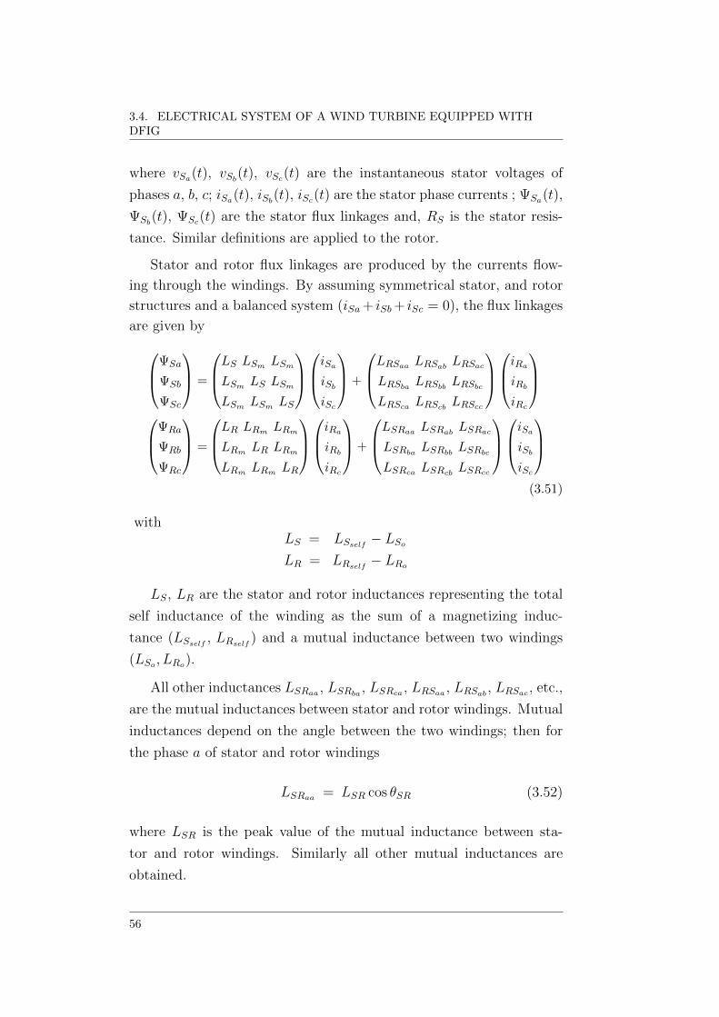
3.4. ELECTRICAL SYSTEM OF A WIND TURBINE EQUIPPED WITHDFIG
where vSa(t), vSb(t), vSc(t) are the instantaneous stator voltages of
phases a, b, c; iSa(t), iSb(t), iSc(t) are the stator phase currents ; ΨSa(t),
ΨSb(t), ΨSc(t) are the stator flux linkages and, RS is the stator resis-
tance. Similar definitions are applied to the rotor.
Stator and rotor flux linkages are produced by the currents flow-
ing through the windings. By assuming symmetrical stator, and rotor
structures and a balanced system (iSa+ iSb+ iSc = 0), the flux linkages
are given byΨSa
ΨSb
ΨSc
=
LS LSm LSm
LSm LS LSm
LSm LSm LS
iSa
iSb
iSc
+
LRSaa LRSabLRSac
LRSbaLRSbb
LRSbc
LRSca LRScbLRScc
iRa
iRb
iRc
ΨRa
ΨRb
ΨRc
=
LR LRm LRm
LRm LR LRm
LRm LRm LR
iRa
iRb
iRc
+
LSRaa LSRabLSRac
LSRbaLSRbb
LSRbc
LSRca LSRcbLSRcc
iSa
iSb
iSc
(3.51)
withLS = LSself
− LSo
LR = LRself− LRo
LS, LR are the stator and rotor inductances representing the total
self inductance of the winding as the sum of a magnetizing induc-
tance (LSself, LRself
) and a mutual inductance between two windings
(LSo , LRo).
All other inductances LSRaa , LSRba, LSRca , LRSaa , LRSab
, LRSac , etc.,
are the mutual inductances between stator and rotor windings. Mutual
inductances depend on the angle between the two windings; then for
the phase a of stator and rotor windings
LSRaa = LSR cos θSR (3.52)
where LSR is the peak value of the mutual inductance between sta-
tor and rotor windings. Similarly all other mutual inductances are
obtained.
56

CHAPTER 3. VARIABLE-SPEED WIND POWER GENERATION SYSTEMS
Equations (3.45)-(3.51) can be written in the general matrix form
as
vS = −dΨS
dt−RS iS
vR = −dΨS
dt−RR iR (3.53)
ΨS = LS iS + LSR iR
ΨR = LR iR + LRS iS (3.54)
where vS, vR, iS, iR are the three-phase voltage and current vectors,
and the matrices LSR = LSR are
LSR = LSR
cos θSR cos(θSR + 2π
3
)cos(θSR − 2π
3
)cos(θSR − 2π
3
)cos θSR cos
(θSR + 2π
3
)cos(θSR + 2π
3
)cos(θSR − 2π
3
)cos θSR
(3.55)
d-q Model
The dynamic equation of a three-phase DFIG can be represented in the
d-q frame since the resultant equations are especially suited for control
and simulation purposes.
The Park transformation can be written as
xdq =
[xd
xq
]= T(θ)
xaxbxc
(3.56)
with
T(θ) = K
sin θ sin(θ − 2π
3) sin(θ + 2π
3)
cos θ cos(θ − 2π3
) cos(θ + 2π3
)1√2
1√2
1√2
(3.57)
where θ is the rotation angle and the factor K is taken as usually√2
3for power invariant transformations.
57

3.4. ELECTRICAL SYSTEM OF A WIND TURBINE EQUIPPED WITHDFIG
By applying the transformation to equations (3.45)-(3.50)
vSd = −RS iSd −dΨSd
dt− ωSΨSq (3.58)
vSq = −RS iSq −dΨSq
dt+ ωSΨSd (3.59)
vRd = RR iRd −dΨRd
dt− s ωSΨRq (3.60)
vRq = −RR iRq −dΨRq
dt+ s ωSΨRd (3.61)
with rotor and stator d-q fluxes given by
ΨSd = LS iSd + Lo iRd (3.62)
ΨSq = LS iSq + Lo iRq (3.63)
ΨRd = LR iRd + Lo iSd (3.64)
ΨRq = LR iRq + Lo iSq (3.65)
Per unit
In order to normalize the electrical system, the power and the voltage
are usually chosen as base quantities; that is to say, equal to one per
unit under rated condition.
The wind turbine electrical system in dq-axis reference frame ((3.58)-
(3.61)) is described in per unit (pu) values based on nominal voltage, on
the three-phase nominal power of the generator, and on the electrical
speed of the generator,
VB =√
3VLLrated[ V ] (3.66)
SB = S3φ,rated [ VA ] (3.67)
ωelB = 2πf
[el.rad
s
](3.68)
where f is the electrical grid frequency in Hz.
58

CHAPTER 3. VARIABLE-SPEED WIND POWER GENERATION SYSTEMS
Thus, the base current and impedance are defined as
IB =SBVB
[A] , ZB = 3V 2B
SB[ Ω ]
The base voltage of low and high voltage side are referred to the
same side by the turns ratio of the transformer. The mechanical and
electrical speeds are related by the pole-pair number as
ωRB =ωelBnpp
[mech.rad
s
](3.69)
The bases of the electromagnetic and turbine torque are given by
TeB = SB/ωRB and TtB = SB/ωtB, respectively, with ωtB = ωRB/ngb
as defined in the previous section. The base torque is in [Nm].
With the per-unit definition in (3.26), stator and rotor voltage equa-
tions in d-q reference frame ((3.58)-(3.61)) in per-unit notation can be
rewritten as
vSd = −RS iSd −1
ωelB
dΨSd
dt− ωSΨSq (3.70)
vSq = −RS iSq −1
ωelB
dΨSq
dt+ ωSΨSd (3.71)
vRd = −RR iRd −1
ωelB
dΨRd
dt− s ωSΨRq (3.72)
vRq = −RR iRq −1
ωelB
dΨRq
dt+ s ωSΨRd (3.73)
ΨSd = LS iSd + Lo iRd (3.74)
ΨSq = LS iSq + Lo iRq (3.75)
ΨRd = LR iRd + Lo iSd (3.76)
ΨRq = LR iRq + Lo iSq (3.77)
Notice that subscript “pu” is not indicated in the previous equations
as the model used in the remainder of this text is expressed in per-unit
(unless otherwise stated).
59
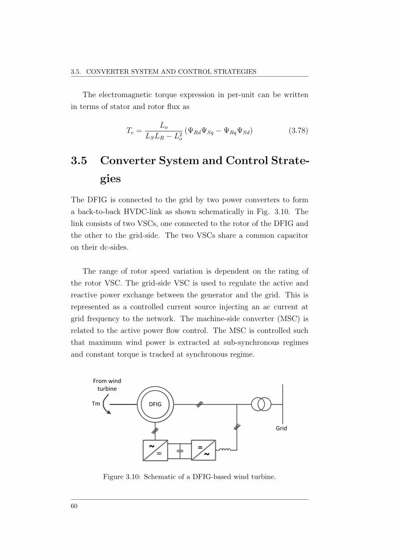
3.5. CONVERTER SYSTEM AND CONTROL STRATEGIES
The electromagnetic torque expression in per-unit can be written
in terms of stator and rotor flux as
Te =Lo
LSLR − L2o
(ΨRdΨSq −ΨRqΨSd) (3.78)
3.5 Converter System and Control Strate-
gies
The DFIG is connected to the grid by two power converters to form
a back-to-back HVDC-link as shown schematically in Fig. 3.10. The
link consists of two VSCs, one connected to the rotor of the DFIG and
the other to the grid-side. The two VSCs share a common capacitor
on their dc-sides.
The range of rotor speed variation is dependent on the rating of
the rotor VSC. The grid-side VSC is used to regulate the active and
reactive power exchange between the generator and the grid. This is
represented as a controlled current source injecting an ac current at
grid frequency to the network. The machine-side converter (MSC) is
related to the active power flow control. The MSC is controlled such
that maximum wind power is extracted at sub-synchronous regimes
and constant torque is tracked at synchronous regime.
Grid
~ ~
DFIGTm
From wind turbine
Figure 3.10: Schematic of a DFIG-based wind turbine.
60

CHAPTER 3. VARIABLE-SPEED WIND POWER GENERATION SYSTEMS
The DFIG converter control has been generally dealt with classical
methods. The most widely employed control techniques are based on
field oriented control (FOC) [91] and direct control techniques like the
direct control torque (DTC), direct self control (DSC) and direct power
control (DPC) [92, 93, 94]. The direct control techniques, as applied
to the DFIG, are based on rotor flux regulation as opposed to stator
flux regulation which applies to squirrel cage induction machine.
Technological advances have lead to develop more efficient strate-
gies based on advanced and modern control techniques such as Fuzzy
Logic Control, Robust Control, Adaptive Control, etc. Among them,
Sliding Mode Control (SMC) emerges as a particularly suitable option
to deal with electronically controlled variable speed operating WECS.
Interest in this control approach has emerged due to its potential to
eliminate the effects of parameter variations with minimum complex-
ity of implementation [6], [7]. The non-linear SMC technique has been
widely applied in variable-speed wind systems but it has been applied
at only the mechanical system, i.e., the thrust has been on power max-
imization and on the pitch controller.
In this thesis a non-linear technique based on Sliding Mode Con-
trol (SMC) is put forward as an alternative approach to control the
converter of a DFIG-based wind system. A FOC based scheme is also
applied as a basis of comparison with the new results obtained with
the proposed SMC.
3.5.1 Machine Side Converter
3.5.2 Field Oriented Control (FOC)
The control of the MSC has been generally carried out by the classical
field-oriented control to carry out a decoupled regulation of active and
reactive power delivery through the stator. In the FOC method, the
active and reactive powers are controlled separately by means of d-q
components of the rotor currents using PI controllers [95].
61
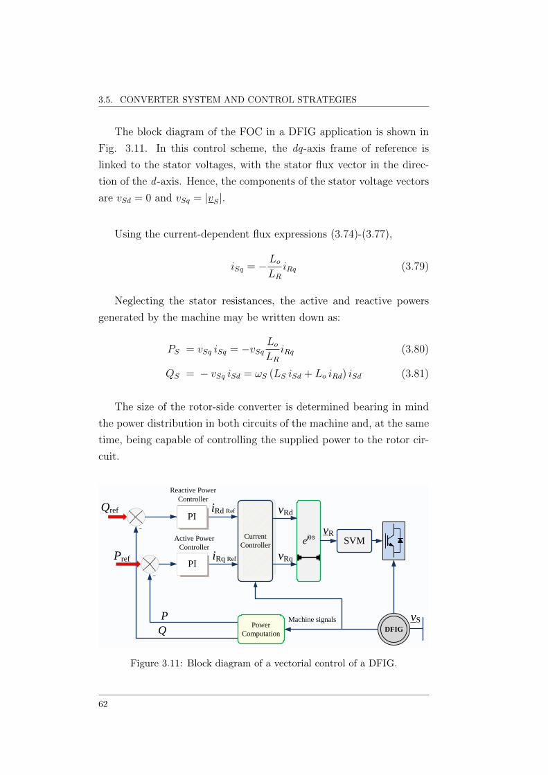
3.5. CONVERTER SYSTEM AND CONTROL STRATEGIES
The block diagram of the FOC in a DFIG application is shown in
Fig. 3.11. In this control scheme, the dq-axis frame of reference is
linked to the stator voltages, with the stator flux vector in the direc-
tion of the d -axis. Hence, the components of the stator voltage vectors
are vSd = 0 and vSq = |vS|.
Using the current-dependent flux expressions (3.74)-(3.77),
iSq = −LoLR
iRq (3.79)
Neglecting the stator resistances, the active and reactive powers
generated by the machine may be written down as:
PS = vSq iSq = −vSqLoLR
iRq (3.80)
QS = − vSq iSd = ωS (LS iSd + Lo iRd) iSd (3.81)
The size of the rotor-side converter is determined bearing in mind
the power distribution in both circuits of the machine and, at the same
time, being capable of controlling the supplied power to the rotor cir-
cuit.
PI
Current
Controllere
jqsSVM
DFIGPower
Computation
Qref
Pref
Reactive Power
Controller
Active Power
Controller
iRd Ref
iRq Ref
vRd
vRq
vR
Machine signals vS
Q
P
-
-
PI
PI
Figure 3.11: Block diagram of a vectorial control of a DFIG.
62

CHAPTER 3. VARIABLE-SPEED WIND POWER GENERATION SYSTEMS
The reference values for the rotor currents are determined from the
steady-state relationship between the rotor and stator currents, with
the stator resistance neglected,
iR =vS
ωS Lo− LSLoiS (3.82)
Assuming known values of the stator reference active and reactive
powers, the corresponding reference currents referring to the rotor are
iRdRef=|vS|ωS Lo
+LS|vS|Lo
QSRef(3.83)
iRqRef= − LS
LoiSq PSRef
(3.84)
The rotor voltage components are obtained from the dynamic equa-
tions of the machine-side controller as follows.
For the d -axis control loop
dXQS
dt= QSRef
−QS = QSerr (3.85)
dXid
dt= KQS
QSerr +KQS
TQS
XQS− iRd (3.86)
uRd = KiddXid
dt+Kid
TidXid (3.87)
For the q-axis control loop
dXP
dt= PRef − P = Perr (3.88)
dXiq
dt= KPPerr +
KP
TPXP − iRq (3.89)
uRq = KiqdXiq
dt+Kiq
TiqXiq (3.90)
where QSerr is the reactive power error; XQSis the state variable
of the outer controller; Xid is the state variable of the inner controller,
Perr is the active power error; XP and Xiq are the state variables of the
outer and inner controllers. The parameters Kid, Kiq, KP , KQSare the
63

3.5. CONVERTER SYSTEM AND CONTROL STRATEGIES
controller proportional gains (P-gains). The parameters Tid , Tiq , TP ,
TQSare the controller reset times or integral times (I-times).
3.5.3 Sliding Mode Control (SMC)
The design of the rotor controller is developed through a theoretical
framework based on the combination of a geometric approach and slid-
ing mode techniques, as put forward in [96]. The key idea of sliding-
mode control (SMC) is to allow a desired performance of the system
to follow a specified sliding surface. Interest in this control approach
has emerged due to its potential to eliminate the effects of parameter
variations with minimum complexity of implementation [6, 7].
Design method
The sliding mode control design consists of two steps:
• First Step: selection of an equilibrium sliding surfaces (x), such
that the internal zero-dynamics is stable and the enforcing sliding
mode in this manifold (x) = 0. Considering the non-linear system
x = Ax+B u+ h
y = s(s)(3.91)
where x ∈ Rn , u(x) ∈ Rm, B(x) ∈ Rnxm, and y ∈ R.
x, u, and B, represent the state, control vectors and control input
matrix, h represents the external uncertainties and disturbances.
The disturbances are assumed to be bounded as follows: |h1| ≤H1, |h2| ≤ H2.
The system (3.91) is transformed to the regular form [6]
x1 = A11 x1 + A12 x2 + h (3.92)
x2 = A21 x1 + A22 x2 +B2 u+ h (3.93)
64

CHAPTER 3. VARIABLE-SPEED WIND POWER GENERATION SYSTEMS
where x1 ∈ Rn−m, x2 ∈ Rm, and B2 is an mxm non-singular
matrix.
Let the tracking error e = x∗ − x where x∗ is the commanded
value. The system can be expressed as
de
dt= e = Ae+B u+ h (3.94)
where h = h− (A− I)x∗.
The sliding mode manifold can be defined as
s = Ce =[F b2
] [e1e2
]= Fe1 + e2 (3.95)
with F ∈ Rmxn The state vector e2 is selected as a function of
the state vector e2 as
e2 = −F e1 (3.96)
Shaping the desired dynamics of the system
e1 = (A11 − A12F )e1 (3.97)
where matrix F is chosen such that AsysSM= A11 − A12F has
stable eigenvalues and the system response has the desired be-
haviour while the system is in sliding mode.
• Second Step: After switching surface design, the next important
aspect is guaranteeing the existence of a sliding mode. These
conditions may be derived from a Lyapunov function
V (x) > 0
V (x) =1
2sT s
(3.98)
The time derivative of V (x) is given by
V (x) =1
2sT∂s
∂xx = sT
∂s
∂x(f(x) +B(x)u) (3.99)
65

3.5. CONVERTER SYSTEM AND CONTROL STRATEGIES
where s =[s1, s2, ..., sm
]Tand
∂s
∂x=
[∂s1∂x
,∂s2∂x
, ...,∂sm∂x
]Tmxn
In order to design a sliding mode control scheme to drive the
system trajectories onto the sliding mode s = 0 for t > 0, it may
be assumed that s(x) = 0 too, and then the equivalent control
law is obtained. From (3.95)
u(x) = −[∂s
∂xB
]−1 [∂s
∂xA
](3.100)
and substituting u(x) into (3.91) to yield the sliding mode dy-
namics as
x = A+B
(−[∂s
∂xB
]−1 [∂s
∂xA
])(3.101)
Sliding surfaces of a DFIG
In a wind turbine DFIG is necessary to regulate both, the active and
the reactive power to a set point ordered by the wind farm control
system. This is so in order to meet the demanded generation control
capability by the grid connection requirements [97, 98].
The block diagram of the SMC in a variable speed wind turbine
application in this research project is shown in Fig. 3.12.
The reference value for the stator active power is determined from
the electromagnetic torque expression given by (3.78) and by the flux-
currents relationship between the rotor and the stator ((3.74)-(3.77)).
The objective of active power control can be set through the indi-
vidual sliding manifold determined by
s1 = PSRef−(−ωS Lo ΨSd ΨRq
σ LS LR
)(3.102)
66

CHAPTER 3. VARIABLE-SPEED WIND POWER GENERATION SYSTEMS
Sliding Mode
Controller ejqs
SVM
DFIGPower
Computation
Qref
Pref
vRd
vRq
vR
Machine signals vS
Q
P
-
-
Figure 3.12: Block diagram of a sliding mode control of a DFIG.
The second objective control is the reactive power tracking, defined
by considering the minimization of the DFIG’s copper losses. It can be
expressed through the following sliding variable:
s2 = QRef −(− Lo |vS| iRdωS (LS + Lo)
− |vS|2
ωS Lo
)(3.103)
3.5.4 Grid Side Converter
Since the DFIG-based wind system is particularly sensitive to volt-
age variations, disturbed grid voltage conditions have to be considered
in the GSC control design. The dc-link voltage is kept constant by
the control of the grid-side converter and ensures steady active power
output from the whole system. As GSC controls affect primarily the
dynamics of dc-link, they are not specifically applied to wind driven
DFIG applications. These dynamic characteristics of the dc link can be
well encapsulated by representing their impact on the DFIG’s rotor by
a dynamic equivalent voltage source, which is a function of the power
balance at the dc bus,
Pdc = Pg + PR (3.104)
Pdc = vdc idc = C vdcdvdcdt
(3.105)
67
--

3.6. CONCLUSIONS
According to the DFIG-converter configuration, it can be stated
that
PR = Poutput − PS (3.106)
Moreover, in accordance with (3.104) and (3.105),
Pg = Poutput − PS (3.107)
the dc link voltage will be kept around its reference value. An ex-
haustive literature search indicates that the GSC controls employ PI
controllers where the dc link voltage and the reactive power are com-
manded by different loop controls.
Regarding reactive power flow control, different operating strategies
may be pursued depending on the sharing of reactive power production
between the DFIG stator and the grid-side converter [91, 99, 100].
Control of the DFIG based on SMC has been addressed both un-
der ideal [101, 102] and unbalanced grid voltage conditions [103, 104].
In [101] a non-linear sliding-mode control scheme was employed in a
direct active and reactive power control (DPC) of a grid-connected
DFIG-based wind turbine system. In [104] a DFIG-based wind turbine
operating under unbalanced and/or harmonically distorted grid voltage
conditions was addressed.
In this work, the control of the GSC is carried out using SMC under
grid disturbances to assess the dynamical control performance of the
DFIG.
3.6 Conclusions
In this chapter a wind turbine system model with double fed induction
generator was presented. The turbine performance was described by
means of the energy conversion theory and general considerations re-
garding simulations for wind turbines in electrical power systems were
68

CHAPTER 3. VARIABLE-SPEED WIND POWER GENERATION SYSTEMS
presented. Simple turbine model assuming constant wind speed, rotor
speed and pitch angle can be used in studies in which the variation in
rotor speed is small as in the case of small disturbance studies with
constant wind speed. However it is not suitable for studies with chang-
ing wind speed or significant rotor speed variation.
Non-linear algebraic models in which power output is obtained from
the wind speed were used in power system stability analysis. The drive
train was modelled by the two-mass model approach in order to rep-
resent correctly the shaft dynamics. The electrical system model was
expressed in per-unit notation and d-q reference frame. The converter
configuration was described and the machine side controller was de-
tailed. The rotor voltage was determined either applying FOC-based
or SMC-based algorithm. In the scheme put forward, the grid-side
converter controls regulate the reactive power which flows through con-
verter to grid and influence mainly the dc-link dynamics by maintaining
the voltage of dc-capacitor into a fixed value.
69

3.6. CONCLUSIONS
70

Chapter 4
Double-fed Induction
Generator Grid Connected
applying Sliding Mode
Control
The small-signal stability assessment of a wind turbine with doubly-fed
induction generator under sliding mode control is carried out in this
chapter. The Double-fed Induction Generator is represented by its sev-
enth order model and subjected to a wide range parameter variation
aiming at carrying out a rather comprehensive dynamic stability assess-
ment of the system. In order to evaluate the impact that controllers
have on the system modes of a Double-fed Induction Generator-based
wind system, the sliding mode control (SMC) algorithm is used and
compared to the classical field-oriented control (FOC).
4.1 Background
Wind energy has shown to be one of the most competitive and effi-
cient renewable energy sources and, as a result, its use is continuously
increasing. It has been reported that in June 2010, the total installed
71

4.1. BACKGROUND
wind energy capacity around the world stood at 175,000 MW [105].
However, incorporation of wind energy units into power networks not
only modifies power flows but may also induce under-voltages or over-
voltages at specific points of the network [106], as well as in certain cases
introduce dynamic stability problems. Doubly-Fed Induction Genera-
tors (DFIG) are the most widespread technology around the world and
they offer the ability of a decoupled PQ control and the possibility of
maintaining their steady state under small perturbations. The increase
of wind energy penetration based on power converters is reducing the
effective inertia of power networks [107], increasing thus the need to
improve the dynamic behaviour of WTs under disturbances.
When performing small signal and transient stability analysis, mod-
els of generators, shafts and their controls must be accurate within the
range of oscillation modes. The use of inaccurate models of equipment
and controls will yield erroneous results in most cases [108]. In [109],
a two-axis model with constant lumped parameters is used for tran-
sient stability analysis in which the mechanical part of the turbine is
all but omitted. Also it is customary to neglect the stator dynamics
[55, 110, 111]. However, the associated modes could have significant
effects on DFIG transient behaviour, as it has been shown in [112].
Classic controllers of DFIGs are usually based on Field Oriented
Control (FOC), where its performance relies on the tuning of the PI
parameters according to the adopted model of the wound induction
machine, the flexible shaft coupling and the converters. Very little re-
search has been done on analyzing the effect of non-linear control on the
improvement of the stability assessment. Technology break-throughs
have allowed the incorporation of advanced control systems into wind
energy generation systems (WECS) and the development of more ef-
ficient strategies based on modern control techniques such as: Fuzzy
Logic Control, Robust Control, Adaptive Control, etc. Among them,
Sliding Mode Control (SMC) emerges as a particularly suitable option
72

CHAPTER 4. DOUBLE-FED INDUCTION GENERATOR GRIDCONNECTED APPLYING SLIDING MODE CONTROL
to deal with electronically controlled variable speed operating WECS.
Interest in this control approach has emerged due to its potential to
eliminate the effects of parameter variations with minimum complex-
ity of implementation [6], [7]. In recent years, the application of SMC
techniques to electrical drives and wind-energy generation [113], [114]
has been studied.
The small-signal stability of a wind turbine with DFIG has been as-
sessed under different operating modes and control tuning [115]. How-
ever, the study was carried out using the 5th reduced order model
(ROM) of the induction generator and the control representation was
simplified and based on decoupled vector control principles.
To overcome these limitations, this study uses a full 7th order DFIG
model. The model comprises the wind turbine, the DFIG and its asso-
ciated back-to-back HVDC link and its associated controls. Connection
of the DFIG to a strong equivalent grid is assumed at this stage of de-
velopment. This study is particularly useful to check the stability of
the DFIG itself and its controls.
The dynamic stability of the system is investigated by eigenvalue
assessment for a wide range of parameter variations. The modal anal-
ysis carried out elucidates the main effects existing on system modes
of a DFIG-based wind system by applying the classical FOC control
and the SMC techniques. This study may form basis on which to es-
tablish guidelines to improve the small-signal stability of DFIG wind
turbines by applying non-linear controls such as the SMC. The results
were obtained with a computer program written in MATLAB.
4.2 Simulation and Results
The small-signal stability of a DFIG directly connected to an equivalent
grid is studied by examining the eigenvalues, eigenvalue properties and
participation factors for a number of different system conditions.
73

4.2. SIMULATION AND RESULTS
The simulation used for this analysis contains models of the turbine,
drive train, generator, electrical network and controllers.
It is important to emphasize how the dynamic behaviour of the
DFIG-based WT system changes under different modes of operation.
First, modal analysis (analysis of eigenvalue locations, eigenvalue
properties and participation factors) of the open-loop DFIG is carried
out to gain a solid understanding of the inherent strengths and weak-
nesses of the system with no control.
From the linearised DAE model (2.8), the system state matrix, Asys
can be obtained:
∆x = Asys ∆x (4.1)
The state vector is defined by
x =[iSd iSq eSd eSq ωt ωR θωt
]T(4.2)
The terminal voltage is 1 pu and remains constant throughout the
simulation. The reactive power output is zero. The parameters of the
DFIG wind turbine system are listed in Table 4.1.
The linearised model (4.1) is used for the small-signal stability anal-
ysis. For the given case of the DFIG-based WT system, the charac-
Table 4.1: DFIG-WT data
DFIG parameters
RS RR Lo Lsl Lrl Hg npp Pwrated
(pu) (pu) (pu) (pu) (pu) (s) (MW)
0.0048 0.0059 3.953 0.092 0.099 2.5 2 2
Ht k c vwratedRblade ngb Cpmax λtipopt
(s) ( puel.rad
) ( pu.sel.rad
) (ms) (m)
0.5 0.3 0.01 17 45 100.5 0.45 7.84
74
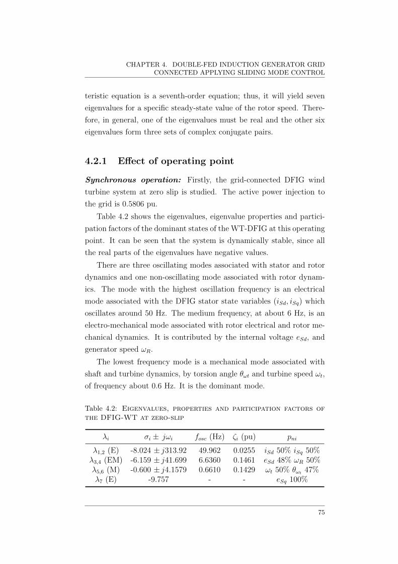
CHAPTER 4. DOUBLE-FED INDUCTION GENERATOR GRIDCONNECTED APPLYING SLIDING MODE CONTROL
teristic equation is a seventh-order equation; thus, it will yield seven
eigenvalues for a specific steady-state value of the rotor speed. There-
fore, in general, one of the eigenvalues must be real and the other six
eigenvalues form three sets of complex conjugate pairs.
4.2.1 Effect of operating point
Synchronous operation: Firstly, the grid-connected DFIG wind
turbine system at zero slip is studied. The active power injection to
the grid is 0.5806 pu.
Table 4.2 shows the eigenvalues, eigenvalue properties and partici-
pation factors of the dominant states of the WT-DFIG at this operating
point. It can be seen that the system is dynamically stable, since all
the real parts of the eigenvalues have negative values.
There are three oscillating modes associated with stator and rotor
dynamics and one non-oscillating mode associated with rotor dynam-
ics. The mode with the highest oscillation frequency is an electrical
mode associated with the DFIG stator state variables (iSd, iSq) which
oscillates around 50 Hz. The medium frequency, at about 6 Hz, is an
electro-mechanical mode associated with rotor electrical and rotor me-
chanical dynamics. It is contributed by the internal voltage eSd, and
generator speed ωR.
The lowest frequency mode is a mechanical mode associated with
shaft and turbine dynamics, by torsion angle θωt and turbine speed ωt,
of frequency about 0.6 Hz. It is the dominant mode.
Table 4.2: Eigenvalues, properties and participation factors ofthe DFIG-WT at zero-slip
λi σi ± jωi fosc (Hz) ζi (pu) pni
λ1,2 (E) -8.024 ± j313.92 49.962 0.0255 iSd 50% iSq 50%λ3,4 (EM) -6.159 ± j41.699 6.6360 0.1461 eSd 48% ωR 50%λ5,6 (M) -0.600 ± j4.1579 0.6610 0.1429 ωt 50% θωt 47%λ7 (E) -9.757 - - eSq 100%
75

4.2. SIMULATION AND RESULTS
The non-oscillating mode is a real eigenvalue associated with rotor
electrical dynamics, by the internal voltage eSq. As it can be seen from
Table 4.2, the λ1,2 is a poorly damped mode (∼ 2.5%). All other modes
are well damped (ζ > 10 %).
Sub/super-synchronous operating: In these cases, the total
active power injected at the point of common coupling is 0.26146 pu at
the sub-synchronous regime and 0.99583 pu at the super-synchronous
regime.
Table 4.3 shows the eigenvalues, eigenvalue properties and par-
ticipation factors of the dominant states of the WT-DFIG at sub-
synchronous speed and Table 4.4 shows similar information but for
the super-synchronous speed. It can be observed that the system is
dynamically stable at both operating modes.
There are three oscillating modes associated with stator and rotor
dynamics and one non-oscillating mode associated with mechanical dy-
namics. The mode with the highest oscillation frequency is an electrical
mode associated with the DFIG stator state variables (iSd, iSq) which
oscillates around 50 Hz. The medium frequency electrical mode, about
12-13 Hz, is associated with the rotor through the dynamics of the
internal voltages eSd and eSq and a small contribution of rotor speed
(∼ 12%).
Table 4.3: Eigenvalues, properties and participation factors ofthe WT-DFIG at sub-synchronous operation
λi σi ± jωi fosc (Hz) ζi (pu) pni
λ1,2 (E) -8.044 ± j313.85 49.951 0.0256 iSd 50% iSq 50%λ3,4 (EM) -8.086 ± j84.031 13.374 0.0957 eSd 50% eSq 40%
ωR 12%λ5,6 (EM) -3.078 ± j8.910 1.418 0.3265 θωt 54% ωR 33%
ωt 10% eSq 8%λ7 (M) -0.881 - - ωt 80% ωR 17%
76
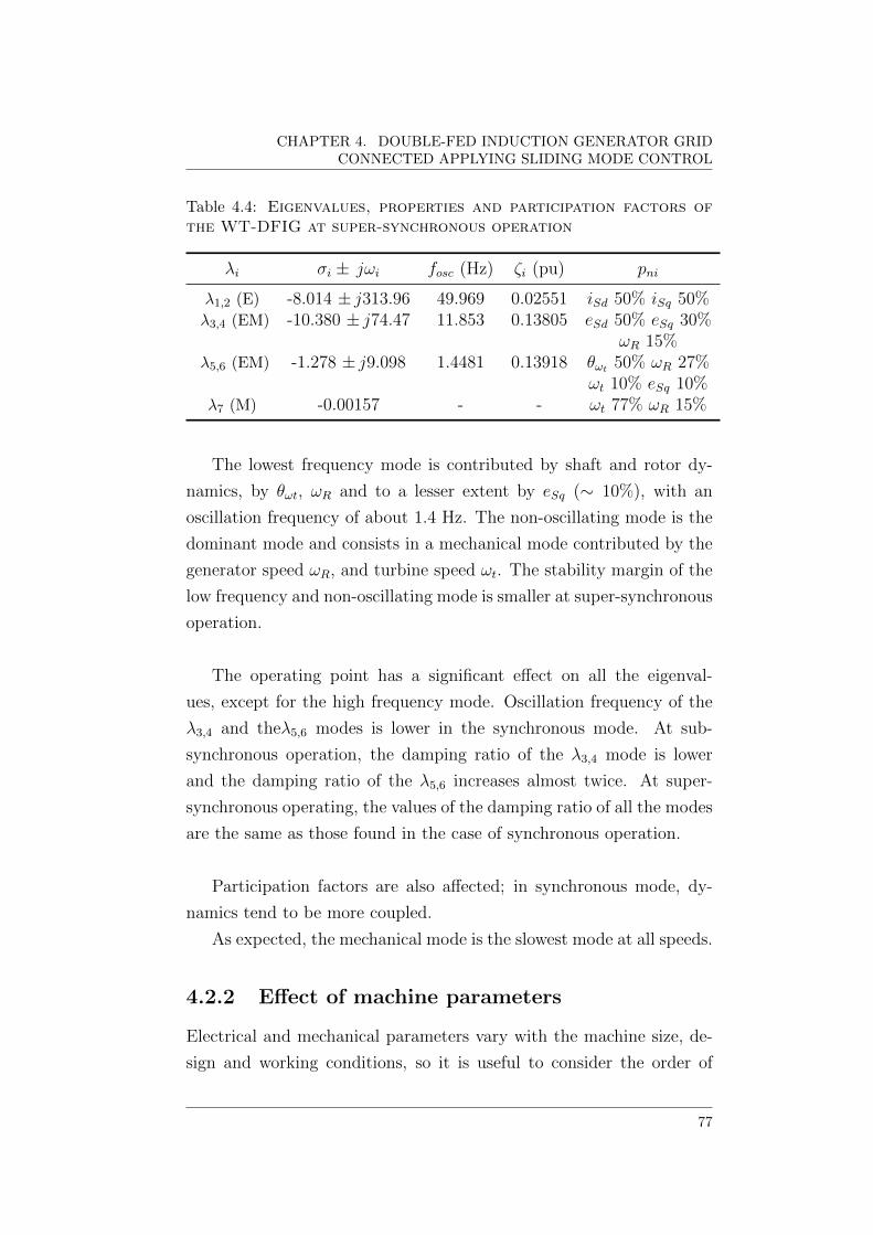
CHAPTER 4. DOUBLE-FED INDUCTION GENERATOR GRIDCONNECTED APPLYING SLIDING MODE CONTROL
Table 4.4: Eigenvalues, properties and participation factors ofthe WT-DFIG at super-synchronous operation
λi σi ± jωi fosc (Hz) ζi (pu) pni
λ1,2 (E) -8.014 ± j313.96 49.969 0.02551 iSd 50% iSq 50%λ3,4 (EM) -10.380 ± j74.47 11.853 0.13805 eSd 50% eSq 30%
ωR 15%λ5,6 (EM) -1.278 ± j9.098 1.4481 0.13918 θωt 50% ωR 27%
ωt 10% eSq 10%λ7 (M) -0.00157 - - ωt 77% ωR 15%
The lowest frequency mode is contributed by shaft and rotor dy-
namics, by θωt, ωR and to a lesser extent by eSq (∼ 10%), with an
oscillation frequency of about 1.4 Hz. The non-oscillating mode is the
dominant mode and consists in a mechanical mode contributed by the
generator speed ωR, and turbine speed ωt. The stability margin of the
low frequency and non-oscillating mode is smaller at super-synchronous
operation.
The operating point has a significant effect on all the eigenval-
ues, except for the high frequency mode. Oscillation frequency of the
λ3,4 and theλ5,6 modes is lower in the synchronous mode. At sub-
synchronous operation, the damping ratio of the λ3,4 mode is lower
and the damping ratio of the λ5,6 increases almost twice. At super-
synchronous operating, the values of the damping ratio of all the modes
are the same as those found in the case of synchronous operation.
Participation factors are also affected; in synchronous mode, dy-
namics tend to be more coupled.
As expected, the mechanical mode is the slowest mode at all speeds.
4.2.2 Effect of machine parameters
Electrical and mechanical parameters vary with the machine size, de-
sign and working conditions, so it is useful to consider the order of
77

4.2. SIMULATION AND RESULTS
magnitude of the various parameters and the extent to which each
parameter influences particular modes.
In this subsection, a modal analysis of DFIG is carried out to inves-
tigate the effect of changing DFIG parameters on eigenvalues and the
degree of participation of state variables in the system modes. Changes
from 0.01% to around 300% in machine parameters were introduced to
assess their impact at different operating modes, i.e., for the whole of
rotor speed range.
Electrical parameters: Stator and rotor machine resis-
tances and magnetization inductance.
The machine resistances RS and RR exert a significant effect on the
open-loop eigenvalue placement and on the participation factor. The
relationship between stator and rotor resistance is RR = 1.2292RS.
Smaller resistance values alter the system stability at non- synchronous
speed. Displacement of real part magnitude of all eigenvalues σi, is di-
rectly proportional to resistances variation, i.e., it tends to increase
negatively with resistance value increases.
The real part magnitudes of the high-frequency and medium-frequency
oscillating modes have an almost linear variation with resistance vari-
ation for the whole operating range. The frequency is affected more
with resistance value increases. The most significant changes are for
the oscillation frequency of the λ3,4 and λ5,6 modes. The oscillation
frequency of λ3,4 decreases up to -4.5% at synchronous speed and the
oscillation frequency of λ5,6 decreases up to -13% (from RS to 3RS) be-
low synchronous speed. The frequency of the λ1,2 is affected to a lesser
extent (∼ −0.5% from RS to 3RS) for the whole operating range. The
damping ratio improves with increasing resistance values.
The main outcomes at both, synchronous and non-synchronous op-
eration are:
At synchronous speed, the system is dynamically stable for the
78
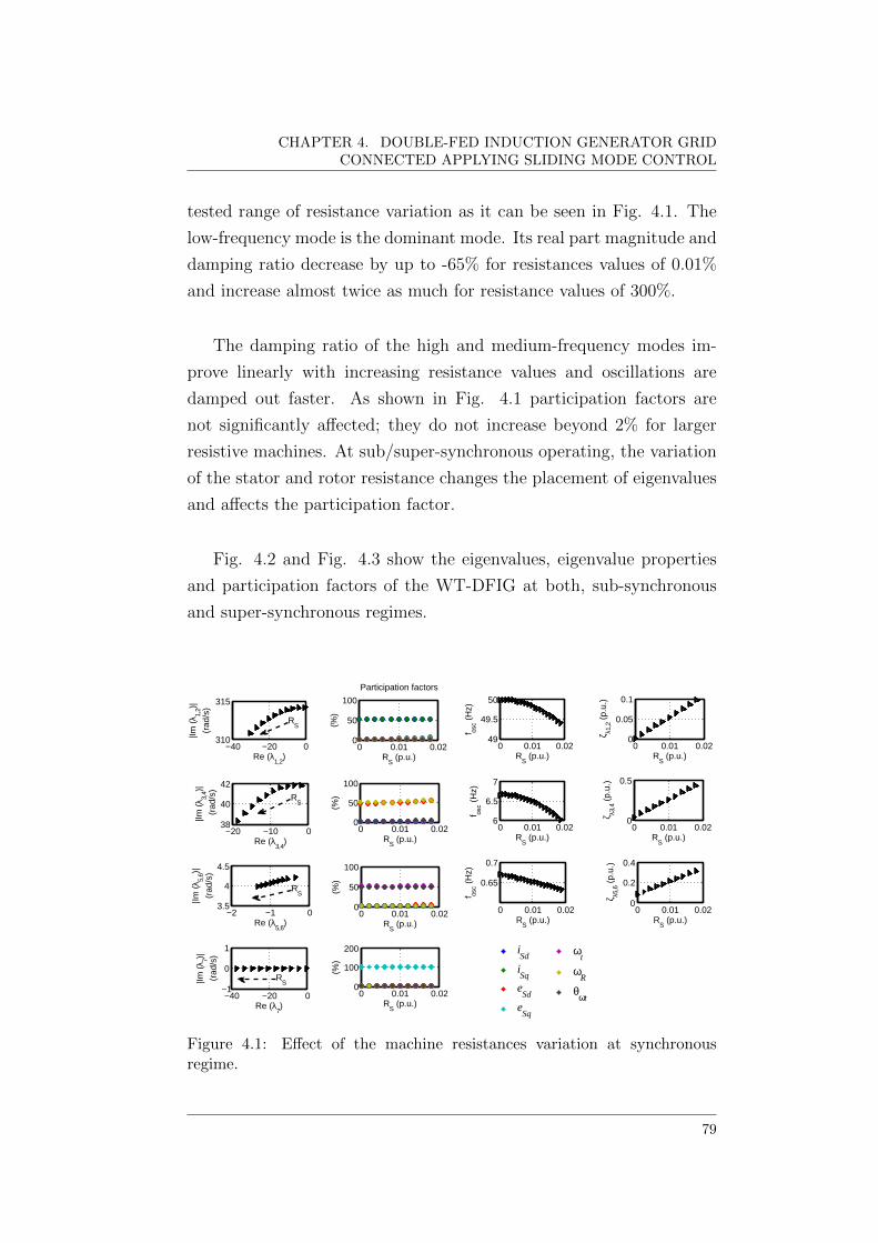
CHAPTER 4. DOUBLE-FED INDUCTION GENERATOR GRIDCONNECTED APPLYING SLIDING MODE CONTROL
tested range of resistance variation as it can be seen in Fig. 4.1. The
low-frequency mode is the dominant mode. Its real part magnitude and
damping ratio decrease by up to -65% for resistances values of 0.01%
and increase almost twice as much for resistance values of 300%.
The damping ratio of the high and medium-frequency modes im-
prove linearly with increasing resistance values and oscillations are
damped out faster. As shown in Fig. 4.1 participation factors are
not significantly affected; they do not increase beyond 2% for larger
resistive machines. At sub/super-synchronous operating, the variation
of the stator and rotor resistance changes the placement of eigenvalues
and affects the participation factor.
Fig. 4.2 and Fig. 4.3 show the eigenvalues, eigenvalue properties
and participation factors of the WT-DFIG at both, sub-synchronous
and super-synchronous regimes.
−40 −20 0310
315
|Im (λ
1,2)|
(rad
/s)
Re (λ1,2
)0 0.01 0.02
0
50
100
RS (p.u.)
(%)
−20 −10 038
40
42
|Im (λ
3,4)|
(ra
d/s)
Re (λ3,4
)
0 0.01 0.020
0.5
RS (p.u.)
ζ λ3,4
(p.
u.)
0 0.01 0.020
50
100
RS (p.u.)
(%)
−40 −20 0−1
0
1
|Im (λ
7)|
(rad
/s)
Re (λ7)
0 0.01 0.020
100
200
RS (p.u.)
(%)
−2 −1 0
4.5
4
3.5
|Im (λ
5,6)|
(rad
/s)
Re (λ5,6
)0 0.01 0.02
0
0.2
0.4
RS (p.u.)
ζ λ5,6
(p.
u.)
0 0.01 0.020
50
100
RS (p.u.)
(%)
0 0.01 0.020
0.05
0.1
RS (p.u.)
ζ λ1,2
(p.
u.)
0 0.01 0.0249
49.5
50
f osc (
Hz)
RS (p.u.)
0 0.01 0.026
6.5
7
f osc (
Hz)
RS (p.u.)
0 0.01 0.02
0.65
0.7
RS (p.u.)
f osc (
Hz)
00.51203040
iSd
iSq
eSd
eSq
−20 20
50100
ωt
ωR
θωt
RS
RS
RS
RS
Participation factors
Figure 4.1: Effect of the machine resistances variation at synchronousregime.
79

4.2. SIMULATION AND RESULTS
−40 −20 0305
310
315
|Im (λ
1,2)|
(rad
/s)
Re (λ1,2
)
−40 −20 080
85
90
|Im (λ
3,4)|
(rad
/s)
Re (λ3,4
)
−8 −6 −4 −2 06
8
10
|Im (λ
5,6)|
(rad
/s)
Re (λ5,6
)
−3 −2 −1 0−1
0
1
Re (λ7)
|Im (λ
7)|
(rad
/s)
0 0.01 0.020
0.05
0.1
RS (p.u.)
ζ λ1,2
(p.
u.)
0 0.01 0.02−0.5
0
0.5
RS (p.u.)
ζ λ3,4
(p.
u.)
0 0.01 0.020
0.5
1
RS (p.u.)
ζ λ5,6
(p.
u.)
0 0.01 0.020
50
100
RS (p.u.)
(%)
0 0.01 0.020
50
100
RS (p.u.)
(%)
0 0.01 0.020
50
100
RS (p.u.)
(%)
0 0.01 0.020
50
100
RS (p.u.)
(%)
0 0.01 0.0249
49.5
50
f osc (
Hz)
RS (p.u.)
0 0.01 0.0213
13.5
14
f osc (
Hz)
RS (p.u.)
0 0.01 0.021
1.5
f osc (
Hz)
RS (p.u.)
−20 20
50100
ωt
ωR
θωt
00.51203040
iSd
iSq
eSd
eSq
RS
RS
RS
RS
Participation factors
Figure 4.2: Effect of machine resistances variation at sub-synchronous op-eration.
−40 −20 0310
315
|Im (λ
1,2)|
(rad
/s)
Re (λ1,2
)
−40 −20 070
75
|Im (λ
3,4)|
(rad
/s)
Re (λ3,4
)
−4 −2 08
9
10
Re (λ5,6
)
|Im (λ
5, 6)|
(rad
/s)
−2 0 2−1
0
1
Re (λ7)
|Im (λ
7)|
(rad
/s)
0 0.01 0.020
0.05
0.1
RS (p.u.)
ζ λ1,2
(p.
u.)
0 0.01 0.020
0.5
ζ λ3,4
(p.
u.)
RS (p.u.)
0 0.01 0.020
0.5
RS (p.u.)
ζ λ5,6
(p.
u.)
0 0.01 0.02−1
0
1
RS (p.u.)
ζ λ7 (
p.u.
)
0 0.01 0.02
49.6
49.8
50
f osc (
Hz)
RS (p.u.)
0 0.01 0.0211
11.5
12
f osc (
Hz)
RS (p.u.)
0 0.01 0.021.3
1.4
1.5
f osc (
Hz)
RS (p.u.)
0 0.01 0.020
50
100
RS (p.u.)
(%)
0 0.01 0.020
50
100
RS (p.u.)
(%)
0 0.01 0.020
50
100
RS (p.u.)
(%)
0 0.01 0.020
50
100
RS (p.u.)
(%)
00.51203040
iSd
iSq
eSd
eSq
−20 20
50100
ωt
ωR
θωt
RS
RS
RS
RS
Participation factors
Figure 4.3: Effect of machine resistances variation at super-synchronousoperation.
80

CHAPTER 4. DOUBLE-FED INDUCTION GENERATOR GRIDCONNECTED APPLYING SLIDING MODE CONTROL
The medium-frequency mode becomes unstable at sub-synchronous
operation if the resistance is neglected. The real part magnitude of
the lowest frequency mode varies ±60% at sub-synchronous operation
within the range of resistance value considered. As the real mode at
non-synchronous operation is the closest to the imaginary axis, it is the
dominant mode. At super-synchronous operation, it has the smallest
stability margin and it becomes unstable for RS < 0.004 pu (below
0.83RS).
As shown in Fig. 4.2, increasing resistance affects the participa-
tion factors of the mechanical and non-oscillating modes. Contribution
of the state variables associated with λ5,6 increases around 10%. The
shaft dynamics, by θωt, increases its participation in the real mode at
sub-synchronous speed. Oscillations are damped out faster for more
resistive machines (above RS).
Variation on magnetization inductance Lo seems to alter only the
stability of the real mode at super-synchronous operation when it in-
creases above 5% (Lo > 4.15 pu), as shown in Figs. 4.4, 4.5 and 4.6.
−15 −10 −540
50
60
|Im (λ
3,4)|
(rad
/s)
Re (λ3,4
)
−20 −15 −10313.8
314
314.2
|Im (λ
1,2)|
(rad
/s)
Re (λ1,2
)
−0.605 −0.6
4.25
4.2
4.15
|Im (λ
5,6)|
(rad
/s)
Re (λ5,6
)
−20 −10 0−1
0
1
Re (λ7)
|Im (λ
7)|
(rad
/s)
0 5 100.02
0.04
0.06
Lo (p.u.)
ζ λ1,2
(p.
u.)
0 5 100.1
0.15
0.2
ζ λ3,4
(p.
u.)
Lo (p.u.)
0 5 100.14
0.142
0.144
ζ λ5,6
(p.
u.)
Lo (p.u.)
0 5 10
49.95
50.1
f osc (
Hz)
Lo (p.u.)
0 5 106
8
10
f osc (
Hz)
Lo (p.u.)
0 5 100.66
0.68
0.7
Lo (p.u.)
f osc (
Hz)
0 5 100
50
100
Lo (p.u.)
(%)
0 5 100
50
100
Lo (p.u.)
(%)
0 5 100
50
100
(%)
Lo (p.u.)
0 5 100
100
200
Lo (p.u.)
(%)
00.51203040
iSd
iSq
eSd
eSq
−20 20
50100
ωt
ωR
θωt
Lo
Lo
Lo
Lo
Participation factors
Figure 4.4: Effect of the leakage inductance variation at synchronous regime.
81
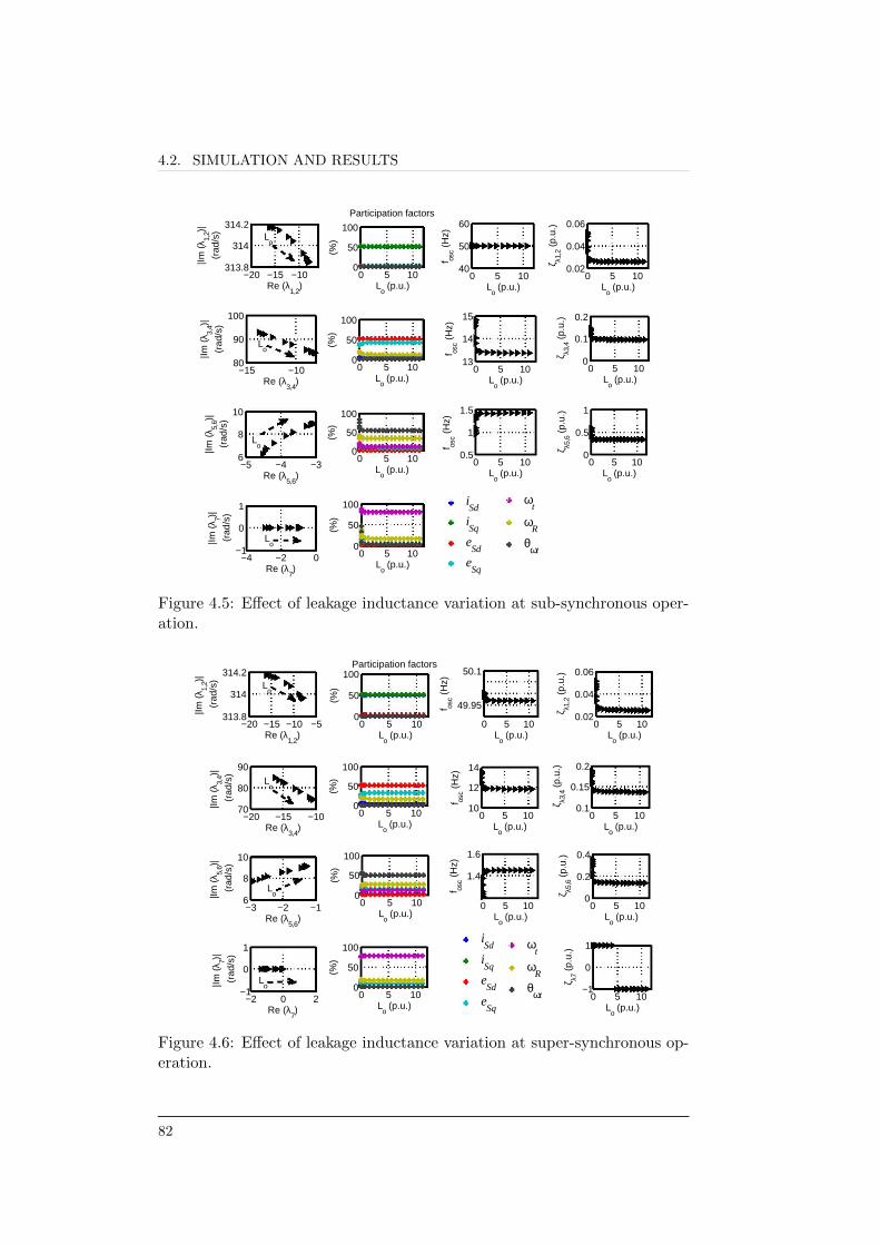
4.2. SIMULATION AND RESULTS
−20 −15 −10313.8
314
314.2
|Im (λ
1,2)|
(rad
/s)
Re (λ1,2
)
−15 −1080
90
100
|Im (λ
3,4)|
(rad
/s)
Re (λ3,4
)
−5 −4 −36
8
10
|Im (λ
5,6)|
(rad
/s)
Re (λ5,6
)
−4 −2 0−1
0
1
Re (λ7)
|Im (λ
7)|
(rad
/s)
0 5 100.02
0.04
0.06
Lo (p.u.)
ζ λ1,2
(p.
u.)
0 5 100
0.1
0.2
ζ λ3,4
(p.
u.)
Lo (p.u.)
0 5 100
0.5
1
Lo (p.u.)
ζ λ5,6
(p.
u.)
0 5 100
50
100
Lo (p.u.)
(%)
0 5 100
50
100
Lo (p.u.)
(%)
0 5 100
50
100
Lo (p.u.)
(%)
0 5 100
50
100
Lo (p.u.)
(%)
0 5 100.5
1
1.5
f osc (
Hz)
Lo (p.u.)
0 5 1013
14
15
f osc (
Hz)
Lo (p.u.)
0 5 1040
50
60
f osc (
Hz)
Lo (p.u.)
00.51203040
iSd
iSq
eSd
eSq
−20 20
50100
ωt
ωR
θωt
Lo
Lo
Lo
Lo
Participation factors
Figure 4.5: Effect of leakage inductance variation at sub-synchronous oper-ation.
−20 −15 −10 −5313.8
314
314.2
Re (λ1,2
)
|Im (λ
1,2)|
(rad
/s)
−20 −15 −1070
80
90
|Im (λ
3,4)|
(rad
/s)
Re (λ3,4
)
−3 −2 −16
8
10
Re (λ5,6
)
|Im (λ
5,6)|
(rad
/s)
−2 0 2−1
0
1
Re (λ7)
|Im (λ
7)|
(rad
/s)
0 5 100
50
100
Lo (p.u.)
(%)
Participation factors
0 5 100
50
100
Lo (p.u.)
(%)
0 5 100
50
100
Lo (p.u.)
(%)
0 5 100
50
100
Lo (p.u.)
(%)
0 5 100.02
0.04
0.06
Lo (p.u.)
ζ λ1,2
(p.
u.)
0 5 100.1
0.15
0.2
ζ λ3,4
(p.
u.)
Lo (p.u.)
0 5 100
0.2
0.4
ζ λ5,6
(p.
u.)
Lo (p.u.)
0 5 10−1
0
1
Lo (p.u.)
ζ λ7 (
p.u.
)
0 5 10
49.95
50.1
f osc (
Hz)
Lo (p.u.)
0 5 1010
12
14
f osc (
Hz)
Lo (p.u.)
0 5 10
1.4
1.6
f osc (
Hz)
Lo (p.u.)
00.51203040
iSd
iSq
eSd
eSq
−20 20
50100
ωt
ωR
θωt
Lo
Lo
Lo
Lo
Figure 4.6: Effect of leakage inductance variation at super-synchronous op-eration.
82
[]]J a aG]
~."".~ •. L... 8·· b:] ... L ... L 8·· ~ ~ . . ...... : .. . ........ ~
CE ~ EJ]~
c:::J ~ : : ~ ~ . .
•
Eft] EE ~G]
Ba ~ EEf]~
rn ¡¡¡¡¡ ffi]~
63...... w: : : 8] ............. . --=... .. . . . . .
•
CHAPTER 4. DOUBLE-FED INDUCTION GENERATOR GRIDCONNECTED APPLYING SLIDING MODE CONTROL
The real part of the rest of the modes does not decrease beyond 1%
with magnetization inductance increases. The effects are significant for
smaller values of Lo below 15 % (Lo < 0.5). The stability margin of all
modes increases 50 %. Hence, the damping ratio increases up to 50 %,
as shown in Fig. 4.4. The oscillation frequency of the lowest frequency
mode increases up to 30 %.
Effects of Lo on eigenvalue properties at both, sub-synchronous and
super-synchronous operation are shown in Figs. 4.5 and 4.6, respec-
tively. The λ1,2 (E) mode is the fastest mode at sub/super-synchronous
regime. Participation factors are influenced only to some extent at
non-synchronous speed. The contribution of generator ωR, to the elec-
tromechanical mode tends to increase; i.e., it tends to an EM mode for
Lo < 0.2 (5%). Concerning the λ5,6 and λ7 modes, the participation
of the associated variables varies by about ±5%. The contribution of
rotor mechanical and shaft dynamics to the λ7 mode increases at sub-
synchronous speed.
Mechanical parameters.
As expected, varying inertia constants and stiffness do not affect
the electrical modes significantly. The relationship between generator
and turbine inertia constants is Hg = 0.2Ht. For heavier machines, the
stability margin tends to decrease, except for the medium-frequency
mode at sub-synchronous speed, which tends to increase (up to ±12%
for 3Ht), and also for the real mode at synchronous operation which
does not change. For the electrical high-frequency mode, changes do
take place in the real part but to a lesser extent, decreasing by about
-0.5% with increases of Ht to 3Ht and increases up to 5% with the
smaller inertia value considered, for whole range speed.
The main effects at synchronous speed, are shown in Fig. 4.7. The
dominant mode is the lowest frequency mode, λ5,6. The imaginary part
tends to decrease with inertia constants increases.
83

4.2. SIMULATION AND RESULTS
−8.4 −8313.9
313.95
Re (λ1,2
)
|Im (λ
1,2)|
(rad
/s)
−15 −10 −50
50
100
|Im (λ
3,4)|
(rad
/s)
Re (λ3,4
)
−2 −1 0−10
−5
0
Re (λ5,6
)
|Im (λ
5,6)|
(rad
/s)
−9.75765 −9.75755−1
0
1
Re (λ7)
|Im (λ
7)|
(rad
/s)
0 2 4 6 80.024
0.026
0.028
Ht (s)
ζ λ1,2
(p.
u.)
0 2 4 6 80
0.2
0.4
ζ λ3,4
(p.
u.)
Ht (s)
0 2 4 6 80
0.2
0.4
ζ λ5,6
(p.
u.)
Ht (s)
0 2 4 6 849.955
49.96
49.965
f osc (
Hz)
Ht (s)
0 2 4 6 80
10
20
f osc (
Hz)
Ht (s)
0 2 4 6 80
50
100
Ht (s)
(%)
0 2 4 6 80
50
100
Ht (s)
(%)
0 2 4 6 80
50
100
Ht (s)
(%)
0 2 4 6 80
100
200
Ht (s)
(%)
0 2 4 6 80
1
2
Ht (s)
f osc (
Hz)
00.51203040
iSd
iSq
eSd
eSq
−20 20
50100
ωt
ωR
θωt
Ht
Ht
Ht
Participation factors
Figure 4.7: Effect of inertia constants variation at synchronous regime.
Therefore, as expected, heavier machines present lower oscillation
frequencies. The oscillation frequency of λ3,4 and λ5,6 modes varies
between 2.2 times and -40% in the range of variation considered for
the inertia constants which go from 0.2Ht to 3Ht.
Fig. 4.7 shows the effects of inertia constants on eigenvalue prop-
erties. It can be observed that the damping ratio of the medium-
frequency mode increases/decreases by about ±5 percent for Ht =
7.5/Ht = 0.5. As expected, the mechanical mode is the slowest mode
and its τ increases with increasing Ht. Its damping ratio goes up to
5% with decreasing Ht. The participation factors do not seem to be
affected at this operating point.
In case of non-synchronous operation, the λ7 mode is the dominant
mode. The stability margin of λ5,6 and λ7 modes reduces by about 60
percent with increases of Ht to 3Ht, as shown in Figs. 4.8 and 4.9.
84
[aJ B mt~
LE E3 tsJ ~
~ .. ~;:;t. ......... ~. : ... : ... :... ~: ........ ~ .. . ~ - " , ,
- - - - - -
1".1 f··M·· ... t : : •
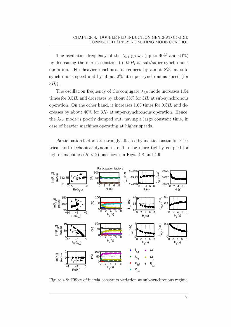
CHAPTER 4. DOUBLE-FED INDUCTION GENERATOR GRIDCONNECTED APPLYING SLIDING MODE CONTROL
The oscillation frequency of the λ3,4 grows (up to 40% and 60%)
by decreasing the inertia constant to 0.5Ht at sub/super-synchronous
operation. For heavier machines, it reduces by about 8%, at sub-
synchronous speed and by about 2% at super-synchronous speed (for
3Ht).
The oscillation frequency of the conjugate λ5,6 mode increases 1.54
times for 0.5Ht and decreases by about 35% for 3Ht at sub-synchronous
operation. On the other hand, it increases 1.63 times for 0.5Ht and de-
creases by about 40% for 3Ht at super-synchronous operation. Hence,
the λ5,6 mode is poorly damped out, having a large constant time, in
case of heavier machines operating at higher speeds.
Participation factors are strongly affected by inertia constants. Elec-
trical and mechanical dynamics tend to be more tightly coupled for
lighter machines (H < 2), as shown in Figs. 4.8 and 4.9.
−8.5 −8313.8
313.85
Re(λ1,2
)
|Im(λ
1,2)|
(rad
/s)
−10 −8 −650
100
150
|Im(λ
3,4)|
(rad
/s)
Re(λ3,4
)
−10 −5 05
10
15
|Im(λ
5,6)|
(rad
/s)
Re(λ5,6
)
−4 −2 0−1
0
1
Re(λ7)
|Im(λ
7)|
(rad
/s)
0 2 4 6 80.024
0.026
0.028
Ht (s)
ζ λ1,2
(p.
u.)
0 2 4 6 80
0.1
0.2
ζ λ3,4
(p.
u.)
Ht (s)
0 2 4 6 80
0.5
Ht (s)
ζ λ5,6
(p.
u.)
0 2 4 6 849.945
49.95
49.955
f osc (
Hz)
Ht (s)
0 2 4 6 810
15
20
f osc (
Hz)
Ht (s)
0 2 4 6 80
2
4
f osc (
Hz)
Ht (s)
0 2 4 6 80
50
100
Ht (s)
(%)
0 2 4 6 80
50
100
Ht (s)
(%)
0 2 4 6 80
50
100
Ht (s)
(%)
0 2 4 6 80
50
100
Ht (s)
(%)
00.51203040
iSd
iSq
eSd
eSq
−20 20
50100
ωt
ωR
θωt
Ht
Ht
Ht
Ht
Participation factors
Figure 4.8: Effect of inertia constants variation at sub-synchronous regime.
85

4.2. SIMULATION AND RESULTS
−8.5 −8 −7.5313.9
313.95
314
Re(λ1,2
)
|Im(λ
1,2)|
(rad
/s)
−20 −10 050
100
150
|Im(λ
3,4)|
(rad
/s)
Re(λ3,4
)
−4 −2 05
10
15
Re(λ5,6
)
|Im(λ
5,6)|
(rad
/s)
−0.01 −0.005 0−1
0
1
Re(λ7)
|Im(λ
7)|
(rad
/s)
0 2 4 6 80
50
100
Ht (s)
(%)
0 2 4 6 80
50
100
Ht (s)
(%)
0 2 4 6 80
50
100
Ht (s)
(%)
0 2 4 6 80
50
100
Ht (s)
(%)
0 2 4 6 80.024
0.026
0.028
Ht (s)
ζ λ1,2
(p.
u.)
0 2 4 6 80.13
0.14
0.15
ζ λ3,4
(p.
u.)
Ht (s)
0 2 4 6 80
0.2
0.4
Ht (s)
ζ λ5,6
(p.
u.)
0 2 4 6 849.965
49.97
49.975
f osc (
Hz)
Ht (s)
0 2 4 6 810
15
20
f osc (
Hz)
Ht (s)
0 2 4 6 80
2
4
f osc (
Hz)
Ht (s)
00.51203040
iSd
iSq
eSd
eSq
−20 20
50100
ω
t
ωR
θωt
Participation factors
Figure 4.9: Effect of inertia constants variation at super-synchronous regime.
Concerning the shaft stiffness variations, changes are significant
only in the medium-frequency and in the low-frequency modes. For
stiffer drive trains, the stability margin of medium-frequency system
modes decreases whereas the low-frequency mode tend to increase. Os-
cillation frequencies increase with k value increases and the damping
ratios deteriorate for the whole range speed. The participation factors
are also affected negatively.
At synchronous speed, the system dynamics change with increasing
shaft stiffness above 6.6k (k > 2), as shown in Fig. 4.10. The dominant
mode changes for stiffer drive trains at this regime, as observed from
the results presented in Fig. 4.10.
With k less than 7.5, the λ5,6 is the dominant mode; otherwise,
the dominance passes onto λ3,4. The λ3,4 mode is the slowest mode
for k > 13. There is an electro-mechanical mode of low oscillation
86
BJ EEB [±±ti ~
BJ &:B [[J]CHíJ
m ea fS ~
Ea ~: : •
•
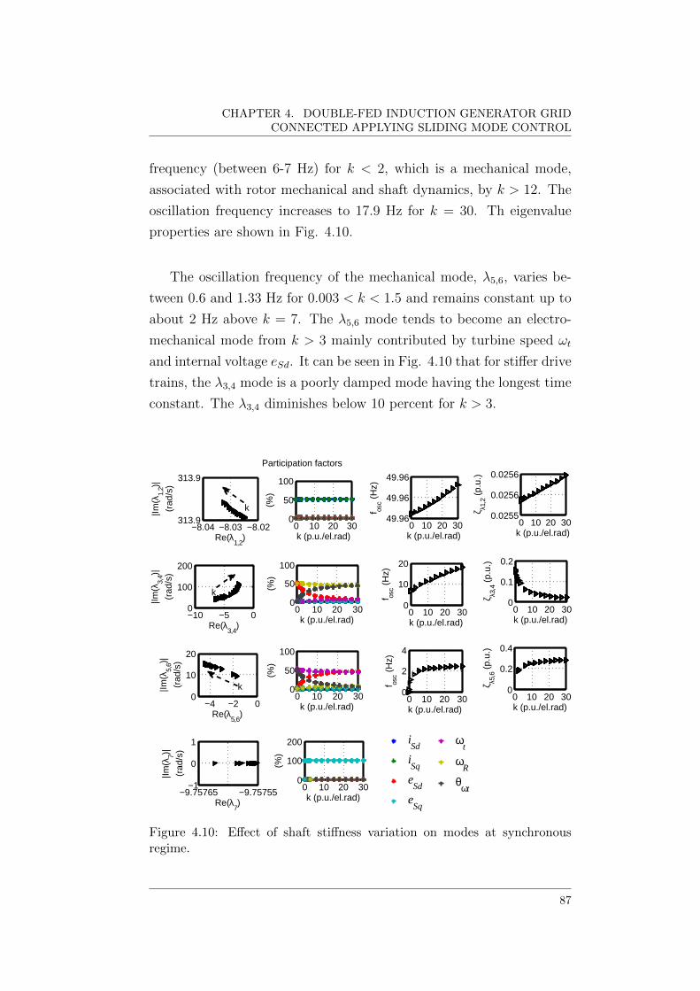
CHAPTER 4. DOUBLE-FED INDUCTION GENERATOR GRIDCONNECTED APPLYING SLIDING MODE CONTROL
frequency (between 6-7 Hz) for k < 2, which is a mechanical mode,
associated with rotor mechanical and shaft dynamics, by k > 12. The
oscillation frequency increases to 17.9 Hz for k = 30. Th eigenvalue
properties are shown in Fig. 4.10.
The oscillation frequency of the mechanical mode, λ5,6, varies be-
tween 0.6 and 1.33 Hz for 0.003 < k < 1.5 and remains constant up to
about 2 Hz above k = 7. The λ5,6 mode tends to become an electro-
mechanical mode from k > 3 mainly contributed by turbine speed ωt
and internal voltage eSd. It can be seen in Fig. 4.10 that for stiffer drive
trains, the λ3,4 mode is a poorly damped mode having the longest time
constant. The λ3,4 diminishes below 10 percent for k > 3.
0 10 20 3049.96
49.96
49.96
f osc (
Hz)
k (p.u./el.rad)0 10 20 30
0.0255
0.0256
0.0256
k (p.u./el.rad)
ζ λ1,2
(p.
u.)
0 10 20 300
10
20
f osc (
Hz)
k (p.u./el.rad)0 10 20 30
0
0.1
0.2
ζ λ3,4
(p.
u.)
k (p.u./el.rad)
0 10 20 300
2
4
f osc (
Hz)
k (p.u./el.rad)0 10 20 30
0
0.2
0.4
k (p.u./el.rad)
ζ λ5,6
(p.
u.)
0 10 20 300
50
100
k (p.u./el.rad)
(%)
0 10 20 300
50
100
k (p.u./el.rad)
(%)
0 10 20 300
50
100
k (p.u./el.rad)
(%)
0 10 20 300
100
200
k (p.u./el.rad)
(%)
−8.04 −8.03 −8.02313.9
313.9
|Im(λ
1,2)|
(rad
/s)
Re(λ1,2
)
−10 −5 00
100
200
|Im(λ
3,4)|
(rad
/s)
Re(λ3,4
)
−4 −2 00
10
20
Re(λ5,6
)
|Im(λ
5,6)|
(rad
/s)
−9.75765 −9.75755−1
0
1
Re(λ7)
|Im(λ
7)|
(rad
/s)
00.51203040
iSd
iSq
eSd
eSq
−20 20
50100
ωt
ωR
θωt
k
k
k
Participation factors
Figure 4.10: Effect of shaft stiffness variation on modes at synchronousregime.
87

4.2. SIMULATION AND RESULTS
At sub/super-synchronous speed, the system dynamics change in
the case of very stiff mechanical systems (k > 23) and are strongly
coupled for 6 < k < 23. The λ7 mode is the dominant mode at both,
sub-synchronous and super-synchronous speed, as shown in Figs. 4.11
and 4.12.
For larger stiffness, the stability margin of λ3,4 is significantly re-
duced (by about 65 percent for k = 30). The λ3,4 mode is an electrical
mode which oscillates with a frequency around 12-13 Hz for k < 2, but
it becomes a mechanical mode with an oscillation frequency between
16-18 Hz, associated with rotor mechanical and shaft dynamics (ωR,
θωt), by k > 23.
For stiffer drive trains, λ3,4 mode is a poorly damped mode having
the longest time constant. Its damping ratio diminishes below 10 per-
cent for k > 9 at super-synchronous speed. The oscillation frequency
of the λ5,6 increases up to around 7-9 Hz for k > 20.
0 10 20 3049.95
49.95
49.95
f osc (
Hz)
k (p.u./el.rad)0 10 20 30
0.0256
0.0256
0.0257
k (p.u./el.rad)
ζ λ1,2
(p.
u.)
0 10 20 3010
15
20
f osc (
Hz)
k (p.u./el.rad)0 10 20 30
0
0.05
0.1
ζ λ3,4
(p.
u.)
k (p.u./el.rad)
0 10 20 300
0.5
1
k (p.u./el.rad)
ζ λ5,6
(p.
u.)
0 10 20 300
50
100
k (p.u./el.rad)
(%)
0 10 20 300
50
100
k (p.u./el.rad)
(%)
0 10 20 300
50
100
k (p.u./el.rad)
(%)
0 10 20 300
50
100
k (p.u./el.rad)
(%)
−8.06 −8.05 −8.04313.85
313.85
313.85
|Im(λ
1,2)|
(rad
/s)
Re(λ1,2
)
−10 −5 080
100
120
|Im(λ
3,4)|
(rad
/s)
Re(λ3,4
)
−10 −5 00
50
100
Re(λ5,6
)
|Im(λ
5,6)|
(rad
/s)
−1 −0.9 −0.8−1
0
1
Re(λ7)
|Im(λ
7)|
(rad
/s)
0 10 20 300
10
20
f osc (
Hz)
k (p.u./el.rad)
0 0.5 1203040
iSd
iSq
eSd
eSq
−20 20
50100
ωt
ωR
θωt
k
k
k
k
Participation factors
Figure 4.11: Effect of shaft stiffness variation on modes at sub-synchronousregime.
88

CHAPTER 4. DOUBLE-FED INDUCTION GENERATOR GRIDCONNECTED APPLYING SLIDING MODE CONTROL
0 10 20 3049.96
49.96
49.96
f osc (
Hz)
k (p.u./el.rad)0 10 20 30
0.0255
0.0255
0.0255
k (p.u./el.rad)
ζ λ1,2
(p.
u.)
0 10 20 3010
15
20
f osc (
Hz)
k (p.u./el.rad)0 10 20 30
0
0.1
0.2
ζ λ3,4
(p.
u.)
k (p.u./el.rad)
0 10 20 300
5
10
f osc (
Hz)
k (p.u./el.rad)0 10 20 30
0
0.5
1
k (p.u./el.rad)
ζ λ5,6
(p.
u.)
−8.02 −8.01313.96
313.96
313.96|Im
(λ1,
2)|
(rad
/s)
Re(λ1,2
)
−12 −9 −6 −350
100
150
|Im(λ
3,4)|
(rad
/s)
Re(λ3,4
)
−6 −4 −2 00
20406080
|Im(λ
5,6)|
(rad
/s)
Re(λ5,6
)
−4 −2 0−1
0
1
Re(λ7)
|Im(λ
7)|
(rad
/s)
0 10 20 300
50
100
k (p.u./el.rad)
(%)
0 10 20 300
50
100
k (p.u./el.rad)
(%)
0 10 20 300
50
100
(%)
k (p.u./el.rad)
0 10 20 300
50
100
k (p.u./el.rad)
(%)
00.51203040
iSd
iSq
eSd
eSq
−20 20
50100
ω
t
ωR
θωt
k
k
k
k
Participation factors
Figure 4.12: Effect of shaft stiffness variation on modes at super-synchronousregime.
4.2.3 Effect of DFIG-order model
A 5th reduced order model (ROM) which does not include the stator
transients has been used by several researches [55, 110, 111].
Table 4.5 shows the modal parameters of the DFIG machine when
a 5th reduced order model is employed. It is noticed that the stability
margin reduces compared to the case when an exact 7th order model is
used (Table 4.2 - 4.4). The electrical high-frequency modes are elimi-
nated.
An important aspect that could be highlighted is the fact that at
super-synchronous regime one of the modes is unstable; however, this
mode does not exist when an exact 7th full-order model is employed.
Furthermore, the effects of the grid should be taken into account for
more accurate results; the dynamics of the machine may be changed
and push some of the modes into the right half plane.
89

4.2. SIMULATION AND RESULTS
Table 4.5: Eigenvalues of the DFIG-WT modelled by a 5th ROM
λi σi ± jωi σi ± jωi σi ± jωi(ωR = 0.7672 p.u ) (ωR = 1 p.u ) (ωR = 1.1981 p.u )
λ3,4 (EM) -4.741 ± j80.26 -5.31 ± j37.072 -10.689 ± j73.323λ5,6 (EM) -3.1343 ± j9.27 -0.617 ± j4.125 -0.588 ± j9.206λ7 (M) -0.817 -7.8287 +0.35455
4.2.4 Effect of grid stiffness
The effect of the grid stiffness is assessed by varying the short circuit
ratio of the grid. The results are shown in Fig. 4.13. It can be seen
that grid impacts mainly the electrical high-frequency mode.
0 10 20−1
0
1
ζ λ1,2
(p.
u.)
Ssc
(p.u.)
0 10 200.12
0.13
0.14
ζ λ3,4
(p.
u.)
Ssc
(p.u.)
0 10 200.1
0.15
0.2
ζ λ5,6
(p.
u.)
Ssc
(p.u.)
0 10 200
50
100
150
f osc
(Hz)
Ssc
(p.u.)
0 10 202
4
6
f osc (
Hz)
Ssc
(p.u.)
0 10 200.5
0.6
0.7
Ssc
(p.u.)
f osc (
Hz)
−20 0 20 40 60 800
250
500
750
Re(λ1,2
)
|Im (λ
1,2)|
(rad
/s)
−4 −3 −210
20
30
Re(λ3,4
)
|Im (λ
3,4)|
(rad
/s)
−0.64 −0.62 −0.63.5
4
4.5
Re(λ5,6
)
|Im (λ
5,6)|
(rad
/s)
−10 −5 0−1
0
1
Re(λ7)
|Im (λ
7)|
(rad
/s)
0 10 200
50
100
Ssc
(p.u.)
(%)
0 10 200
50
100
Ssc
(p.u.)
(%)
0 10 200
50
Ssc
(p.u.)
(%)
0 10 200
100
200
Ssc
(p.u.)
(%)
00.51203040
iSd
iSq
eSd
eSq
−20 20
50100
ωt
ωR
θωt
Ssc
Ssc
Ssc
Ssc
Participation factors
Figure 4.13: Effect of short circuit ratio variation at zero-slip.
90
CHAPTER 4. DOUBLE-FED INDUCTION GENERATOR GRIDCONNECTED APPLYING SLIDING MODE CONTROL
Larger values of short circuit ratio Ssc slide the highest frequency
mode (stator electrical mode) into the right half plane. Hence, the
more inductive the external grid the more the need arises for series
compensation or other controls measures in order to diminish the ef-
fective value of the equivalent inductance.
In case of a strong external networks, the high-frequency electrical
dynamics decay quite fast. For the medium-frequency mode (rotor
electro-mechanical mode), the damping ratio decreases with decreasing
Ssc.
The low-frequency mode (turbine mechanical mode) is, relatively
speaking, less sensitive to external line parameters. This is to be ex-
pected since the grid impedance is an electrical parameter. The non-
oscillating mode (rotor electrical mode) is a real eigenvalue closer to
the imaginary axis for large values of Ssc.
Participation factors are not significantly affected by grid strength.
Although frequency and damping ratio change, the stator mode re-
mains decoupled from the other modes, a situation that applies to
both, strong and weak grids cases.
4.2.5 Influence of the control strategy
To assess the effect of the machine-side controller on local modes, two
different control algorithms are applied to the 7th full-order model
DFIG wind turbine model. The control algorithms are the so-called
FOC and SMC. The study is carried out for the whole range of rotor
speed.
The WT-DFIG system under FOC is in fact an eleventh-order
model. The state vector is defined by
x =[iSd iSq eSd eSq ωt ωR θωt xc
]T(4.3)
91

4.2. SIMULATION AND RESULTS
with
xc =[Φid Φiq ΦTe ΦQs
]Twhere xc is the state vector of the machine-side converter controller.
The state vector of the WT-DFIG system under SMC is defined by
(4.2).
Tables 4.6 and 4.7 show the eigenvalues, properties and the par-
ticipation factors of dominant states of the WT-DFIG system under
FOC. There are two oscillating modes. The highest frequency mode,
unlike the mode in open-loop, is associated with a coupling between
the q-axis stator current component (iSq) and rotor electrical dynamics
(eSd), but it should be notice that the damping ratio is lower.
The lowest frequency mode is a mechanical mode contributed by
θωt and ωR, oscillating with a frequency of around 1.6 Hz with an
acceptable damping (> 10%).
Table 4.6: Eigenvalues and properties of the WT-DFIG withfield-oriented control (FOC)
ωR = 0.91535 p.u. ωR = 1 p.u. ωR = 1.1981 p.u.mode λi λi λi
# ( fosc (Hz), ζi (pu)) ( fosc (Hz), ζi (pu)) ( fosc (Hz), ζi (pu))
λ1 -14780 -15139 -14554λ2 -3391.2 -3636.7 -3634.5λ3,4 -25.815 ± j292 -17.668 ± j289.75 -10.403 ± j292.12
(46.47, 0.08806) ( 46.11, 0.06086) (46.49, 0.03559)λ5 -438.71 -435.88 -440.29λ6 -180.57 -188.73 -195.12λ7 -22.69 -23.715 -23.734λ8,9 -1.8849 ± j10.466 -1.8903 ± j10.465 -1.895 ± j10.464
(1.66 ,0.1772) (1.66, 0.1777) (1.66, 0.1781)λ10 -0.0884 -0.1004 -0.1128λ11 -6.234 -6.667 -6.641
92

CHAPTER 4. DOUBLE-FED INDUCTION GENERATOR GRIDCONNECTED APPLYING SLIDING MODE CONTROL
Table 4.7: Participation factors of the modes of the WT-DFIGwith field-oriented control (FOC)
mode Dom. States# pni
λ1 iSd 100%λ2 iSq 100%λ3,4 eSq 48%, eSd 47%λ5 Φiq 100%λ6 Φid 95%λ7 ΦTe 99%λ8,9 ωR 42%, θωt 50%λ10 ωt 83%, ωR 16%λ11 ΦQs 99%
Below synchronous speed, the mechanical mode, associated with ro-
tor and turbine dynamics, moves close to zero, i.e., the stability margin
decreases with decreasing rotor speed.
The modes associated with the controller depend on the tuning of
the proportional-integral (PI) controllers. For example, it can be cou-
pled with the state variables of the machine.
Eigenvalues, eigenvalue properties and participation factors of the
dominant modes in a WT-DFIG system under SMC are shown in Ta-
bles 4.8 and 4.9. It can be observed that there are two conjugated
modes and that there are no electro-mechanical modes as it was the
case with FOC.
The highest frequency mode, which is associated with electrical
dynamics by iSq and eSq, oscillates with a frequency of around 50 Hz.
Its damping is much improved compared to the one obtained with FOC.
The oscillating mechanical mode is a well damped out mode associated
with shaft and rotor mechanical dynamics, θωt and ωR. It oscillates
with a frequency of around 1.6 Hz.
There are no modes associated with the controller.
93
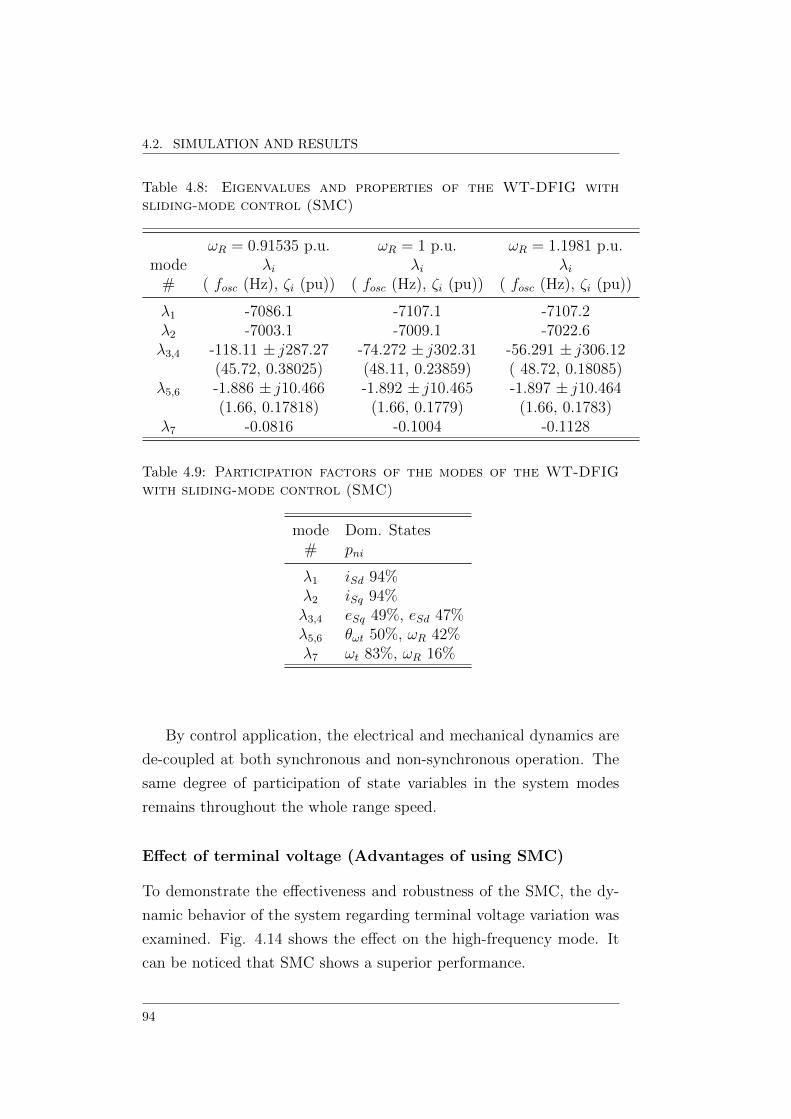
4.2. SIMULATION AND RESULTS
Table 4.8: Eigenvalues and properties of the WT-DFIG withsliding-mode control (SMC)
ωR = 0.91535 p.u. ωR = 1 p.u. ωR = 1.1981 p.u.mode λi λi λi
# ( fosc (Hz), ζi (pu)) ( fosc (Hz), ζi (pu)) ( fosc (Hz), ζi (pu))
λ1 -7086.1 -7107.1 -7107.2λ2 -7003.1 -7009.1 -7022.6λ3,4 -118.11 ± j287.27 -74.272 ± j302.31 -56.291 ± j306.12
(45.72, 0.38025) (48.11, 0.23859) ( 48.72, 0.18085)λ5,6 -1.886 ± j10.466 -1.892 ± j10.465 -1.897 ± j10.464
(1.66, 0.17818) (1.66, 0.1779) (1.66, 0.1783)λ7 -0.0816 -0.1004 -0.1128
Table 4.9: Participation factors of the modes of the WT-DFIGwith sliding-mode control (SMC)
mode Dom. States# pni
λ1 iSd 94%λ2 iSq 94%λ3,4 eSq 49%, eSd 47%λ5,6 θωt 50%, ωR 42%λ7 ωt 83%, ωR 16%
By control application, the electrical and mechanical dynamics are
de-coupled at both synchronous and non-synchronous operation. The
same degree of participation of state variables in the system modes
remains throughout the whole range speed.
Effect of terminal voltage (Advantages of using SMC)
To demonstrate the effectiveness and robustness of the SMC, the dy-
namic behavior of the system regarding terminal voltage variation was
examined. Fig. 4.14 shows the effect on the high-frequency mode. It
can be noticed that SMC shows a superior performance.
94
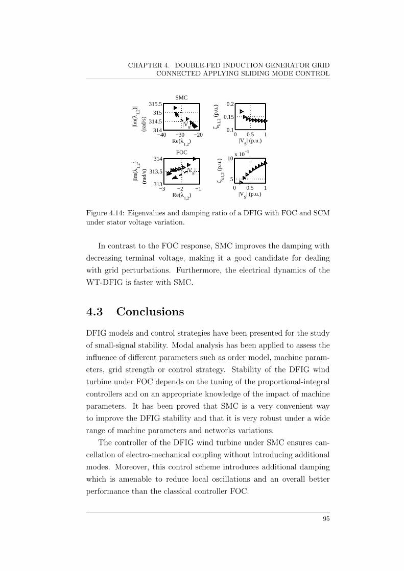
CHAPTER 4. DOUBLE-FED INDUCTION GENERATOR GRIDCONNECTED APPLYING SLIDING MODE CONTROL
−40 −30 −20314
314.5
315
315.5
Re(λ1,2
)|Im
(λ1,
2)|
(ra
d/s)
SMC
0 0.5 10.1
0.15
0.2
ζ λ1,2
(p.
u.)
|VS| (p.u.)
−3 −2 −1313
313.5
314
Re(λ1,2
)
|Im(λ
1,2)
| (ra
d/s)
FOC
0 0.5 1
5
10x 10
−3
ζ λ1,2
(p.
u.)
|VS| (p.u.)
|VS|
|VS|
Figure 4.14: Eigenvalues and damping ratio of a DFIG with FOC and SCMunder stator voltage variation.
In contrast to the FOC response, SMC improves the damping with
decreasing terminal voltage, making it a good candidate for dealing
with grid perturbations. Furthermore, the electrical dynamics of the
WT-DFIG is faster with SMC.
4.3 Conclusions
DFIG models and control strategies have been presented for the study
of small-signal stability. Modal analysis has been applied to assess the
influence of different parameters such as order model, machine param-
eters, grid strength or control strategy. Stability of the DFIG wind
turbine under FOC depends on the tuning of the proportional-integral
controllers and on an appropriate knowledge of the impact of machine
parameters. It has been proved that SMC is a very convenient way
to improve the DFIG stability and that it is very robust under a wide
range of machine parameters and networks variations.
The controller of the DFIG wind turbine under SMC ensures can-
cellation of electro-mechanical coupling without introducing additional
modes. Moreover, this control scheme introduces additional damping
which is amenable to reduce local oscillations and an overall better
performance than the classical controller FOC.
95
~: ~ .... l( .•.. ~.... ..~:: ...... . :~

4.3. CONCLUSIONS
96

Chapter 5
Stability Analysis of
Multi-machine Systems with
Wind Power Generation
All the studies presented in this chapter focus on assessing the impact
of double-fed induction generators on oscillatory stability. The key
factors influencing the system inherent oscillations are brought to the
fore. Then, the main contributing factors of the double-fed induction
generator to system stability are drawn by using modal analysis.
Throughout the chapter, a wide range of simulations are used to
show by numerical example the prowess of the concepts and meth-
ods put forward in this research. Two different power systems are
used: a three-machine system and a four-machine, two-area system.
These enable a good understanding of the electromechanical oscilla-
tions phenomenon and illustrate rather well the improvements that
can be achieved by using DFIG-based wind turbine controllers.
A small signal stability analysis is carried out for two scenarios.
Firstly, all generators are considered to be conventional synchronous
generators and, secondly, one of the synchronous generator is replaced
by one DFIG-based wind farm which, in turn, is controlled by two
different control schemes. One of them is the well-known and widely
implemented Field Oriented Control FOC algorithm; the other is based
97

5.1. BACKGROUND
on a robust design technique termed Sliding Mode Control SMC. The
latter represents a relatively new control application in the area of wind
energy which is rapidly gaining adepts.
The first scenario is used to provide a base line case against which
the impact of wind generation on the network dynamics, can be quan-
tified with a degree of realism.
5.1 Background
The subject of power system stability has received a great deal of at-
tention for decades. In the open literature, the phenomenon of stability
in multi-machine power systems has been addressed from great many
angles by hundreds of researchers. Over the years the research has
addressed issues such as model development, power system equipment
and topologies, control methods, system operating conditions, solution
methods and many other issues.
Operation and dynamics characteristics of systems comprising syn-
chronous generation are already well established and understood. More-
over, due to the tendency to operate systems near their stability limits,
additional schemes have been added to maintain the system dynamics
at acceptable levels. All this has increased further the awareness of
power system oscillation and has provided the motivation to develop
new technology to keep them at bay. A good example of this is the use
of power electronic devices, referred to as FACTS (flexible AC trans-
mission systems) devices [116, 117, 118].
Dynamic studies of mixed synchronous and induction generators is
an issue that is receiving increasing attention, particularly over the last
decade, as the growing penetration levels of DFIGs has increased.
Key contributions have been made toward the understanding of the
interaction of conventional generation with wind power generation by
resorting of transient and modal analysis studies.
98
CHAPTER 5. STABILITY ANALYSIS OF MULTI-MACHINE SYSTEMSWITH WIND POWER GENERATION
In one of the early works [90], the dynamic and transient stability
properties of wind turbine generators integrated into a power system
were explored. The study addressed both, single and grouped wind
turbines subjected to the influence of electrical and wind speed dis-
turbances. Further studies on the dynamic characteristics of electrical
networks with wind energy generation can be found in [52],[111].
The dynamic properties of electrical networks with wind generation
seem to acquire a degree of improvement compared to those systems
with no wind generation. One plausible explanations is that the de-
mands on synchronous generators becomes less onerous with increases
in wind energy, particularly under heavy wind regimes. In addition,
from the DFIG-based wind turbines point of view, the decoupling ca-
pability of the power electronic converter control does not introduce
new oscillatory modes and, consequently, this prevents the wind tur-
bine from being involved in power system oscillations.
A topic that is becoming increasingly important in the field of power
system stability is related to small signal stability of grid-connected
wind power generation [4, 52, 119, 120]. In particular, the damping
of oscillations which characterizes the phenomena of stability has seen
increased research activity in recent years [74, 115, 119, 120, 121, 122,
123]. A point of great relevance has been the influence of increased
DFIG penetration on the stability of inter-area oscillations.
It is shown in [120] that the effect of increased DFIG penetration
is generally favorable since the damping of the inter-area oscillation
increases. However, there are certain cases where the wind turbine is
in voltage control mode and the system becomes stiffer, resulting in
a less well damped inter-area mode which may even become unstable.
Therefore an appropriate controller tuning of the voltage/VAR control
loop is necessary to avoid instability.
An assessment of the impact of eigenvalues location of inter-area
modes has been addressed by conducting a study of wind power level
variations, [4, 52, 54, 74, 119]. Careful observation of the movement of
99
5.1. BACKGROUND
the eigenvalues through the complex plane, lead to the conclusion that
for high levels of wind power penetration the dynamic performance is
superior since the eigenvalue damping increases and the dynamic re-
sponse of the frequency improves [74]. Further evidence of this was
presented in [54], in connection with the impact that a large wind farm
exerts on the oscillation modes of a two-area, four-generator power
system. The study indicates that the inter-area mode tends to become
more stable as the wind generator approaches its rated power, whereas
the opposite is true for systems with synchronous generator.
It has been further verified in [4] that a small increase of both
damping and frequency occurs for the inter-area modes by increasing
gradually the wind power and by reducing, by the same amount, con-
ventional power production, within the same area. However, it was
also observed from several patterns of increasing wind power and load,
that damping reduces whit wind power increases and contributes to
congestion in weak interconnection lines, i.e. when increasing wind
power generation pushes the power system stress level up [124].
In [121], the affected modes by inertia changes (due to the premise
that the increased penetration of DFIG-based wind farms reduces the
system inertia) are identified and then excited by introducing appro-
priate disturbances. The method suitably identifies the benefits and
drawbacks of increasing DFIG penetration from the vantage of small
signal stability and related studies.
Other interesting proposals have been put forward to enhance the
system dynamic performance. By way of example,the use of power
system stabilizers (PSSs) in DFIGs has been proposed recently [55,
122, 125, 126, 127]. The authors in [55] quite insightfully identified
the control capabilities of the DFIG and put forward the idea of a
power system stabilizer for a wind turbine employing the DFIG; they
showed that the PSS can significantly influence the contribution that
100

CHAPTER 5. STABILITY ANALYSIS OF MULTI-MACHINE SYSTEMSWITH WIND POWER GENERATION
a DFIG-based wind farm can make to network damping. The power
system stabilizer was designed to operate with a flux magnitude and
angle controller (FMAC) scheme, where the terminal voltage and sta-
tor power output can be controlled through the magnitude of the rotor
flux vector and its angular position.
In [128] and [129] other types of PSS configurations and controllers
for DFIGs were also introduced. In [128] a conventional PSS was com-
pared with two other PSSs in which their output signals were added
to the power and to the voltage side of the DFIG control system, re-
spectively. It was concluded that a DFIG fitted with the capability to
improve PSS to improve the damping of inter-area power system os-
cillations and that the wind farm may have the potential to positively
contribute to power system damping. The impact of the voltage con-
trol loop on system dynamic performance is examined in [129]. It was
found that besides the penetration level, this control loop has the great-
est impact on inter-area oscillations in comparison with other control
loops such as phase-locked loop (PLL) and pitch angle control, which
exerts a negligible impact.
Since the active and reactive power of variable-speed wind turbines
can be modulated to damp power system oscillations [123], auxiliary
controllers with power modulation (active, reactive or a combination
thereof) have been employed. Power damping control is achieved by
adding auxiliary corrective signals to the control of the machine side
converter of a DFIG-based wind turbine.
In [125], it is pointed out that by active power modulation, ad-
ditional damping to inter-area oscillations can be introduced. The
proposed active power modulation is accomplished by introducing a
supplemental signal at the control loops which contains the inter-area
oscillation information. Results demonstrated that with proper control,
DFIGs have the capability to damp inter-area oscillations. However,
101
5.1. BACKGROUND
one potential disadvantage of active power modulation of wind gener-
ation is its interaction with torsional dynamics of the wind turbines,
since the active power is directly related to the electromagnetic torque.
If P modulation yields oscillations of low-frequency in wind genera-
tors, these may interact with torsional oscillation because of theirs
low-frequency oscillations. This concern, already addressed in [126],
led to the outcome that the damping of the shaft mode decreases due
to active power modulation in wind farms while reactive power modu-
lation is immune to such risk.
Likewise, a combined PSS and active damping controller by eigen-
structure assignment to improve both, the DFIG shaft oscillation and
the power system electromechanical damping was a worthwhile contri-
bution put forward in [127]. The authors demonstrated the use and
capability of the method via its application to the design of a DFIG
controller required to improve both, the damping of DFIG shaft oscil-
latory modes and the network electromechanical damping.
In [122], a coordinated tuning of the damping controller to enhance
the damping of the oscillatory modes by using a bacteria foraging tech-
nique was developed. However, the study was limited to a single DFIG
WT system connected to an infinite bus. Hence, extensions to a multi-
machine DFIG system should be made to quantify the actual impact
of DFIGs on power system stability.
It is stated in [130] that the PSS function in variable-speed wind
generators does not actually require the use of compensators to pro-
duce damping torque due to the fast action of power electronic con-
verter controllers. However, it is possible to increase the selectivity of
the modal damping capabilities and to reduce the sensitivity to distur-
bances through the use of tuned filters. PSS functions based on the
energy function approach (EFA-PSS) and frequency deviation (WPSS),
are normally used in VSC-HVDC and FACTS devices, and may also be
102
CHAPTER 5. STABILITY ANALYSIS OF MULTI-MACHINE SYSTEMSWITH WIND POWER GENERATION
used in this application. The energy function method consists of defin-
ing a function to represent the energy in the system, which is composed
of kinetic and potential energy. The gradient of this energy is mini-
mized by active and reactive power control laws. Both PSS controllers
use active and reactive power modulation.
Similar damping capabilities of wind farms with both PSS functions
are given but both require high proportional gains. On the other hand,
with the tubed Band-Pass Filter in the WPSS, the reactive power con-
trol loop of the EFA-PSS showed vulnerability to voltage disturbances,
which can limit the proportional gain. Active power modulation is
more effective if the PCC of the DFIG-based wind farm is located elec-
trically close to a synchronous generator plant. The opposite holds for
reactive modulation but it requires a large reactive power modulation.
By careful examination of results pertaining to the various scenarios,
it was observed that the amount of PQ modulation impacts directly
the damping potential. Moreover, it was noticed that with a broader
distribution of wind resources, the damping capabilities of the PSS
controller increase while the real and reactive power modulation level
decrease.
Nevertheless, in spite of the fact that the design methodologies for
active and reactive power modulation-based PSSs have great potential,
published work on PSSs remains scant [123].
5.2 The Three-Machine, Nine-Bus System
The nine-bus power system of the Western Systems Coordinating Coun-
cil (WSCC) [24] shown in Fig 5.1 is used as the first test case. It com-
prises three generators, three loads, three transformer and six trans-
mission lines.
Generator 1 is a hydro-generator. Generator 3 is a steam-generator
and Generator 2 is a double fed induction generator (DFIG) although
Generator 2 is considered first to be a steam turbine-driven synchronous
103

5.2. THE THREE-MACHINE, NINE-BUS SYSTEM
generator in order to provide a baseline case against which to compare
the impact on the network dynamic performance, by the wind genera-
tor. The loads are modelled as constant power load type.
The synchronous generators are represented by their two-axis model
and fitted with an IEEE Type I exciter (slow acting with low gain),
shown in Fig. 5.2. The fourth-order two-axis model in the dq frame
is described by equations (5.1)-(5.4). Equations (5.5)-(5.7) are the
differential equations for the IEEE Type I exciter (Fig. 5.2).
dδidt
= ωSGi− ωe (5.1)
2Hi
ωe
dωSGi
dt= TMi − E ′diIdi − E ′qiIqi −
(X ′qi −X ′di
)IdiIqi − . . .
. . .−Di (ωSGi− ωe) (5.2)
T ′qoiE ′didt
= − E ′di +(Xqi −X ′qi
)Iqi (5.3)
T ′doiE ′qidt
= − E ′qi + (Xdi −X ′di) Idi + Efdi (5.4)
1
2 3
4
5 6
7 8 9
Slack
Bus
16.5 kV
230 kV
18 kV 13.8 kV
G2
G1
G3
L5 L6
L8
Figure 5.1: 3-Machine, 9-Bus System
104

CHAPTER 5. STABILITY ANALYSIS OF MULTI-MACHINE SYSTEMSWITH WIND POWER GENERATION
1 AK
FsK
VR
Vs
refV
V
Efd
S (E )E fd
K + sTE E1 + sTA
1 + sTF
Figure 5.2: IEEE Type I exciter
TEi
Efdidt
= − (KEi+ SEi
)Efdi + VRi(5.5)
TFi
Rfi
dt= −Rfi +
KFi
TFi
Efdi (5.6)
TAi
VRi
dt= − VRi
+KAiRfi −
KAiKFi
TFi
Efdi + . . .
. . .+KAi(Vrefi − VSGi
+ Vsi) (5.7)
The exciter is assumed to be identical for all three machines. Power
System Stabilizers (PSS) were not employed in this model so as to en-
able a more straightforward assessment of the impact of Generator 2.
The machine data and the exciter data are given in Table 5.1.
The double fed induction generator is modelled by a 7th order model
as described in Chapter 3. The electrical and mechanical data for the
DFIG-WT are given in Table 5.1.
The system MVA base is 100, and the system frequency is 50 Hz.
The rated power of generators is: Generator 1 = 247.5 MVA, Generator
2 = 192 MVA, and Generator 3 = 128 MVA.
The impedances are in per unit on the system 100 MVA base and
are given in Table 5.2. The power flow solution for the nominal case,
is shown in Table 5.3.
105

5.2. THE THREE-MACHINE, NINE-BUS SYSTEM
Table 5.1: Machines Data
Generator Data
Bus Xd Xq X′d X
′q T
′do T
′qo H D
# (pu) (pu) (pu) (pu) (s) (s) (s)
1 0.146 0.0969 0.0608 0.0969 8.96 0.31 23.64 0.02542 0.8958 0.8645 0.1198 0.1969 6.0 0.535 6.4 0.00663 1.3125 1.2578 0.1813 0.25 5.89 0.6 33.01 0.0026
Exciter Data
KA TA KE TE KF TF Aexc Bexc
(s) (s) (s)
20 0.2 1 0.314 0.063 10.35 0.0039 1.555
DFIG parameters
RS RR Lo Lsl Lrl Hg npp Pwrated
(pu) (pu) (pu) (pu) (pu) (s) (MW)
0.0048 0.0059 3.953 0.092 0.099 2.5 2 2
Ht k c vwrated Rblade ngb Cpmax λtipopt
(s) ( puel.rad) ( pu.s
el.rad) (ms ) (m)
0.5 0.3 0.01 17 45 100.5 0.45 7.84
Table 5.2: System data for the 3-machine System (Fig. 5.1)
System line data
From bus To bus R X Bc (total)
1 4 0.00 0.0576 0.00
7 2 0.00 0.0625 0.00
3 9 0.00 0.0586 0.00
4 6 0.0170 0.0920 0.158
9 6 0.0390 0.1700 0.358
9 8 0.0119 0.1008 0.209
7 8 0.0085 0.0720 0.149
7 5 0.0320 0.1610 0.306
5 4 0.0100 0.0850 0.176
106
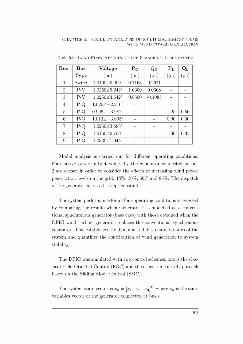
CHAPTER 5. STABILITY ANALYSIS OF MULTI-MACHINE SYSTEMSWITH WIND POWER GENERATION
Table 5.3: Load Flow Results of the 3-machine, 9 bus system
Bus Bus Voltage PG QG PL QL
Type (pu) (pu) (pu) (pu) (pu)
1 Swing 1.0400∠0.000 0.7163 0.2671 - -
2 P-V 1.0250∠9.242 1.6300 0.0668 - -
3 P-V 1.0250∠4.642 0.8500 -0.1085 - -
4 P-Q 1.026∠−2.216 - - - -
5 P-Q 0.996∠−3.982 - - 1.25 0.50
6 P-Q 1.013∠−3.693 - - 0.90 0.30
7 P-Q 1.0260∠3.685 - - - -
8 P-Q 1.0160∠0.700 - - 1.00 0.35
9 P-Q 1.0330∠1.945 - - - -
Modal analysis is carried out for different operating conditions.
Four active power output values by the generator connected at bus
2 are chosen in order to consider the effects of increasing wind power
penetration levels on the grid: 15%, 30%, 50% and 85%. The dispatch
of the generator at bus 3 is kept constant.
The system performance for all four operating conditions is assessed
by comparing the results when Generator 2 is modelled as a conven-
tional synchronous generator (base case) with those obtained when the
DFIG wind turbine generator replaces the conventional synchronous
generator. This establishes the dynamic stability characteristics of the
system and quantifies the contribution of wind generation to system
stability.
The DFIG was simulated with two control schemes, one is the clas-
sical Field Oriented Control (FOC) and the other is a control approach
based on the Sliding Mode Control (SMC).
The system state vector is xn = [x1 x2 x3]T , where xn is the state
variables vector of the generator connected at bus i.
107

5.2. THE THREE-MACHINE, NINE-BUS SYSTEM
The state vector of the synchronous generator is made up of the
states of the two-axis model as well as the state variables of the exciter
model
xSG =[δ ω E ′d E ′q Efd Rf VR
]T(5.8)
where three last three states correspond to the exciter model.
The state variables vector of the DFIG WT takes of the form
xWT =[iSd iSq eSd eSq ωt ωR θωt xc
]T(5.9)
with xc being the state vector of the DFIG controller.
The order of the state variables vector for the DFIG depends on
the order of the type of applied control strategy. This is detailed in
Chapter 3.
For each operating condition two cases are analyzed:
a. Power network with no wind generation
In this case the eigenvalue analysis is performed assuming that all
three generation units are conventional synchronous generators.
The system is a 21th order one,
xSGn =[δi ωi E ′di E ′qi Efdi Rfi VRi
]T(5.10)
for i = 1, 2, 3.
b. Power network with wind generation
In these studies the generator at bus 2 is assumed to be a DFIG-
based wind farm and two different controllers are utilized, namely
FOC and SMC. When the FOC-based controller is used, the sys-
tem is a 24th order system with the following state variables
xn =[xSGi
xWT
]T(5.11)
108

CHAPTER 5. STABILITY ANALYSIS OF MULTI-MACHINE SYSTEMSWITH WIND POWER GENERATION
with xSGibeing the state vector of the synchronous generators
for i = 1, 2 and, xWT = being the state vector of the DFIG-based
wind turbine given by (5.9), where xc =[Xid Xiq XTe XQS
]Tare the state variables of the FOC-based controller.
When the SMC-based controller is used, the system is a 21th order
system with the state vector given by equation (5.11) where xWT
is a 7th order system.
5.2.1 Power Network with no Wind Generation
An electrical power system in which the exported power is supplied by
a conventional synchronous generator is considered first to provide a
base line against which wind penetration studies can be assessed.
Table 5.4 summarizes all the relevant information concerning the
small-signal study for this case. It can be noticed that the system is
stable.
This test system shows two rotor angle oscillations (λ1,2 andλ3,4)
and one real rotor speed mode (λ19). The 1.74 Hz mode λ3,4 corre-
sponds to rotor speed of the machines 3 and 2, where the machine 3
is dominant, and the 1.17 Hz mode λ1,2 is related to machines 1 and
2, with the latter providing most of the contribution. This is the least
damped mode with a damping ratio of 4.395%.
The real rotor speed mode, λ19, contributed by machines 1 and 2,
depends mainly on the rotor speed of machine 1.
The rest of the modes are the local and inter-machine modes as-
sociated with excitation control. The exciter’s modes are all very well
damped. The zero eigenvalue is not shown.
109

5.2.T
HE
TH
RE
E-M
AC
HIN
E,
NIN
E-B
US
SY
ST
EM
Table 5.4: System Modes of the 3-machine system: Two-axis Synchronous Generator with IEEE I exciter
Mode Eigenvalue Frequency Damping Dominant Machine Participation# σi ± jωi f (Hz) ratio ζ(pu) states at bus factor (%)
λ1,2 -0.3261 ± j7.4138 1.1799 0.04395 δ, ω 2 31.6, 31.71 13.4, 13.4
λ3,4 -0.9092 ± j10.982 1.7479 0.08250 δ, ω 3 41.5, 41.52 9.5, 9.5
λ5,6 -5.6101 ± j7.9667 1.2679 0.57576 VR, Efd, Rf 2 45.6, 45.1, 13.0λ7,8 -5.2139 ± j7.8330 1.2467 0.55410 VR, Efd, Rf 1 45.7, 44.4, 13.8λ9,10 -5.4107 ± j7.9291 1.2619 0.56366 VR, Efd, Rf 3 45.1, 44.2, 13.5λ11 -5.3428 - - E ′d 2 53.58
3 49.0λ12 -4.0872 - - E ′d 3 53.4
2 47.8λ13,14 -0.3891 ± j1.1145 0.17738 0.32967 E ′q, Rf 1 29.9, 21.7
2 16.8, 12.4λ15,16 -0.3830 ± j0.7370 0.11731 0.46110 E ′q, Rf 1 25.5, 19.0
2 23.3, 18.2λ17,18 -0.3136 ± j0.5031 0.08007 0.52899 E ′q, Rf 3 37.7, 32.3
2 18.5, 13.2λ19 -0.1645 - - ω 1 72.4
2 18.6λ20 -3.2258 - - E ′d 1 100
110

CHAPTER 5. STABILITY ANALYSIS OF MULTI-MACHINE SYSTEMSWITH WIND POWER GENERATION
Fig. 5.3, describes the eigenvalues movement of the two rotor angle
oscillatory modes λ1,2 and λ3,4 for the 9 bus system when the active
power output of the generator 2 changes from 15% to 85%; four levels
are considered: 15%, 30%, 50%, 85%.
The top two figures of Fig. 5.3 show the eigenvalues movement and
their respective participation factors are shown in the lower row. The
arrow indicates the direction of increasing power output.
From the participation factors results, it can be observed that the
xn state variable contribution changes little at all the various operating
conditions considered, namely (15%, 30%, 50% and 85% of Generator
2’s power output.
−1.05 −1 −0.95 −0.9 −0.8510.5
11
11.5
σ (s−1)
| ω |
(ra
d/s)
λ1,2
−1 −0.8 −0.6 −0.4 −0.26.5
7
7.5λ
3,4
σ (s−1)
| ω |
(ra
d/s)
0 2 4 6 8 1012141618200
20
40
60
State variable x i
Par
ticip
atio
n fa
ctor
(%
)
0 2 4 6 8 1012141618200
20
40
60
State variable x i
%
ω2δ
2
ω1
δ1
ω3δ
3
δ2 ω
2
15% 30% 50%
85% 15%
30%
50%85%
Figure 5.3: Impact of power output of G2 on the swing-rotor modes of theWSCC system. The upper figures depict the eigenvalues movement and; thelower figures the participation factors.
111

5.2. THE THREE-MACHINE, NINE-BUS SYSTEM
The small-signal stability margin of the rotor-speed oscillations,
which is understood to be the distance of the real-part of the eigen-
values (stable eigenvalues with negative real-part) measured from the
imaginary axis of the complex plane; decreases with progressive in-
creases of active power (Fig. 5.3).
The real part magnitude of the inter-machine mode, λ1,2, decreases
up to 65% from lower to higher power whilst the real part magnitude
of the mode λ3,4, decreases up to 15%. Hence, the damping is reduced
from 13.2% to 4.4% and, from 9.17% to 8.25%, respectively (Fig. 5.4).
The oscillation frequencies of the modes, as shown in Fig. 5.4 (left),
are affected little by power generation changes, with the variation being
less than 5% between the two extreme operating conditions (15% and
85% of P of G2).
0 1 2
15 %
30 %
50 %
85 %
f (Hz)
Pow
er o
utpu
t of G
2 Oscillation frequency λ3,4
0 5 10
15 %
30 %
50 %
85 %
ζ (%)
Pow
er o
utpu
t of G
2 Damping ratio λ3,4
0 0.5 1 1.5
15 %
30 %
50 %
85 %
f (Hz)
Pow
er o
utpu
t of G
2
Oscillation frequency λ1,2
0 3 6 9 12 15
15 %
30 %
50 %
85 %
ζ (%)
Pow
er o
utpu
t of G
2
Damping ratio λ1,2
Figure 5.4: Properties of the swing-rotor modes of the WSCC system withactive power output of G2 increases . The upper figures depict the eigenvalueproperties of the λ1,2 mode and; the lower figures depict the eigenvalueproperties of the λ3,4 mode.
112

CHAPTER 5. STABILITY ANALYSIS OF MULTI-MACHINE SYSTEMSWITH WIND POWER GENERATION
5.2.2 Power Network with Wind Generation
In these studies the generator connected at bus 2 is now assumed to be
a DFIG-based wind farm. The DFIG is fitted with the two distinct con-
trol strategies, which have been introduced in previous chapters. The
first one is based on the conventional Field Oriented Control (FOC)
and the second is based on the robust design technique Sliding Mode
Control (SMC).
The benefits of using mixed power generation, involving conven-
tional synchronous generators and DFIG WT, is assessed below, with
two different kinds of DFIG controls being implemented.
Three cases are singled out for analyses:
Case 1: All three generators G1, G2, G3 are of the conventional syn-
chronous generation type
Case 2: G2 represents wind generation with a DFIG-WT with FOC
Case 3: G2 represents wind generation with a DFIG-WT with SMC
The damping ratio is the key parameter with which to assess the
impact that the DFIG has on the dynamics of the system.
Under this scenario, depicted in Fig. 5.5, the system shows two
rotor angle oscillations (λ1,2, λ3,4): λ1,2 relating to the machine con-
nected at bus 1 and, λ3,4 relating to the machine connected at bus 3.
The upper figures (first row) depict the eigenvalues movement and the
lower figures the participation factors corresponding to Case 2: Gener-
ator 2 is a DFIG-WT with FOC, (middle row figures ) and for Case 3:
Generator 2 is a DFIG-WT with SMC, (bottom row figures).
Firstly, it can be seen that the system stability is strongly affected
by the operating point. The oscillatory modes tend to become more
stable as the wind power penetration increases; this is in contrast to
113

5.2. THE THREE-MACHINE, NINE-BUS SYSTEM
the base case (power network with no wind generation), where the sys-
tem stability margin decreases with output power generation increases
(Fig. 5.3, top).
As expected, oscillations associated to the machine 2 only exist in
the base case (with no wind generation).
−0.4 −0.2 0
1.5
2
2.5
3
| ω |
(rad
/s)
σ (s−1)
λ1,2
−0.4 −0.2 02.2
2.4
2.6
PG2
= 15% PG2
= 30% PG2
= 50% PG2
= 85%
−0.62 −0.6 −0.58 −0.56
9
10
11
12λ
3,4
σ (s−1)
| ω |
(rad
/s)
DFIG−WT SMC
DFIG−WT FOC
DFIG−WT FOC
DFIG−WT SMC
0 2 4 6 8 10 12 14 16 18 20 22 240
20
40
60
80
Par
ticip
atio
n fa
ctor
(%
)
λ1,2
0 2 4 6 8 10 12 14 16 18 20 22 240
20
40
60
80λ
3,4
0 2 4 6 8 10 12 14 16 18 200
20
40
60
80
State variable x n
0 2 4 6 8 10 12 14 16 18 200
20
40
60
80
State variable x n
δ1ω
1
ωt
δ3ω
3
ω3
δ3
ωt
ω1δ
1
DFIG−WT FOC DFIG−WT FOC
DFIG−WT SMCDFIG−WT SMC
Figure 5.5: Impact of increasing wind power penetration on the swing-rotoroscillatory modes of the 9 bus system. The upper figures (first row) depictthe eigenvalues movement and the lower figures the participation factorscorresponding to the case 2, ( middle row figures) and the case 3, (bottomrow figures).
114
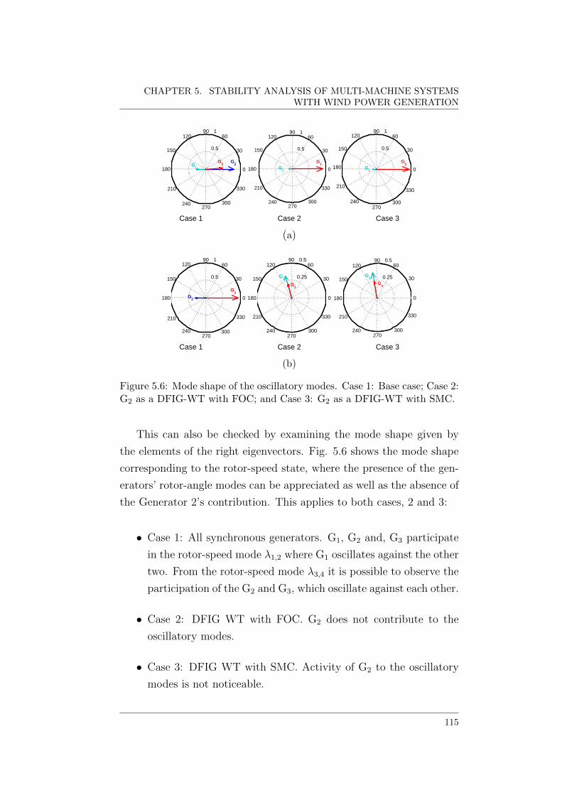
CHAPTER 5. STABILITY ANALYSIS OF MULTI-MACHINE SYSTEMSWITH WIND POWER GENERATION
0.5
1
30
210
60
240
90
270
120
300
150
330
180 0
P2 = 84.375 %
G3
G2G
1
0.5
1
30
210
60
240
90
270
120
300
150
330
180 0
P2 = 84.375% DFIG with VOC
G3
G1
0.5
1
30
210
60
240
90
270
120
300
150
330
180 0
P2 = 84.375% DFIG with SMC
G3
G1
0.5
1
30
210
60
240
90
270
120
300
150
330
180 0
P2 = 84.375%
G3
G2
0.25
0.5
30
210
60
240
90
270
120
300
150
330
180 0
P2 = 84.375% DFIG with VOC
G1
G3
0.25
0.5
30
210
60
240
90
270
120
300
150
330
180 0
P2 = 84.375% DFIG with SMC
G1
G3
Case 1 Case 2 Case 3
(a)
0.5
1
30
210
60
240
90
270
120
300
150
330
180 0
P2 = 84.375 %
G3
G2G
1
0.5
1
30
210
60
240
90
270
120
300
150
330
180 0
P2 = 84.375% DFIG with VOC
G3
G1
0.5
1
30
210
60
240
90
270
120
300
150
330
180 0
P2 = 84.375% DFIG with SMC
G3
G1
0.5
1
30
210
60
240
90
270
120
300
150
330
180 0
P2 = 84.375%
G3
G2
0.25
0.5
30
210
60
240
90
270
120
300
150
330
180 0
P2 = 84.375% DFIG with VOC
G1
G3
0.25
0.5
30
210
60
240
90
270
120
300
150
330
180 0
P2 = 84.375% DFIG with SMC
G1
G3
Case 1 Case 2 Case 3
(b)
Figure 5.6: Mode shape of the oscillatory modes. Case 1: Base case; Case 2:G2 as a DFIG-WT with FOC; and Case 3: G2 as a DFIG-WT with SMC.
This can also be checked by examining the mode shape given by
the elements of the right eigenvectors. Fig. 5.6 shows the mode shape
corresponding to the rotor-speed state, where the presence of the gen-
erators’ rotor-angle modes can be appreciated as well as the absence of
the Generator 2’s contribution. This applies to both cases, 2 and 3:
• Case 1: All synchronous generators. G1, G2 and, G3 participate
in the rotor-speed mode λ1,2 where G1 oscillates against the other
two. From the rotor-speed mode λ3,4 it is possible to observe the
participation of the G2 and G3, which oscillate against each other.
• Case 2: DFIG WT with FOC. G2 does not contribute to the
oscillatory modes.
• Case 3: DFIG WT with SMC. Activity of G2 to the oscillatory
modes is not noticeable.
115

5.2. THE THREE-MACHINE, NINE-BUS SYSTEM
0 0.3 0.6 0.9 1.2f (Hz)
Oscillation frequency λ
1,2
0 3 6 9 12 15ζ (%)
Damping ratio λ
1,2
Case 1Case 2Case 3Case 1Case 2Case 3Case 1Case 2Case 3Case 1Case 2Case 3
PG2
=85%
PG2
=50%
PG2
=30%
PG2
=15%
0 0.5 1 1.5 2f (Hz)
Oscillation frequency λ
3,4
0 2 4 6 8 10ζ (%)
Damping ratio λ
3,4Case 1Case 2Case 3Case 1Case 2Case 3Case 1Case 2Case 3Case 1Case 2Case 3
(a) (b)
Figure 5.7: Eigenvalues properties of the a) mode λ1,2; b) mode λ3,4; of the 9bus system with wind power penetration increases. Case 1: Base case; Case2: G2 as a DFIG-WT with FOC controller; and Case 3: G2 as a DFIG-WTwith SMC controller.
The relevant property modes of the wind power penetration and
the DFIG controller type are shown in Fig. 5.7. This figure shows
the oscillation frequencies of the swing-rotor modes (left plot) and the
damping ratios (right plot).
The mode λ1,2,corresponds to the machine at bus 1 which oscillates
with a frequency close to one-third the frequency in the base case (case
1). It can be seen that for Case 3, when the DFIG-WT is controlled
by SMC, there is an enhancement of the mode damping of up to 5%
compared to the one obtained by FOC in Case 2.
The oscillation frequency of mode λ3,4, associated to Generator 3,
in Fig. 5.7(b), is about 10% higher than when Generator 2 is a syn-
chronous generator. The reason is that the hydro-turbine unit is quite
heavy and the contribution of Generator 2 to this mode in the base
case is quite marginal, as it can be observed from Fig. 5.3. Likewise,
the damping ratio is around 2% better than the base case.
This case has furnished preliminary results that show that a DFIG
WT with SMC yields excellent results in small-signal stability assess-
116
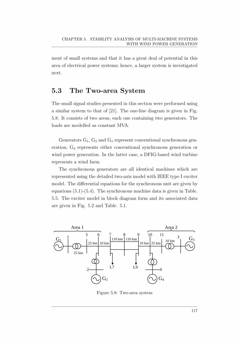
CHAPTER 5. STABILITY ANALYSIS OF MULTI-MACHINE SYSTEMSWITH WIND POWER GENERATION
ment of small systems and that it has a great deal of potential in this
area of electrical power systems; hence, a larger system is investigated
next.
5.3 The Two-area System
The small signal studies presented in this section were performed using
a similar system to that of [21]. The one-line diagram is given in Fig.
5.8. It consists of two areas, each one containing two generators. The
loads are modelled as constant MVA.
Generators G1, G3 and G4 represent conventional synchronous gen-
eration; G2 represents either conventional synchronous generation or
wind power generation. In the latter case, a DFIG-based wind turbine
represents a wind farm.
The synchronous generators are all identical machines which are
represented using the detailed two-axis model with IEEE type I exciter
model. The differential equations for the synchronous unit are given by
equations (5.1)-(5.4). The synchronous machine data is given in Table.
5.5. The exciter model in block diagram form and its associated data
are given in Fig. 5.2 and Table. 5.1.
2
3
4
5 6 7 8 9 101
25 km
10 km110 kmG1
G2
G3
G4
L7 L9
Area 1 Area 2
25 km 10 km110 km
10 km25 km
11
Figure 5.8: Two-area system
117

5.3. THE TWO-AREA SYSTEM
Table 5.5: Machine Data in per unit on the rated MVA base
Rs Xd Xq X′
d X′q T
′
do T′qo H D
0.00028 1.8 1.7 0.3 0.55 8.0 0.4 54 0.0
Both, the synchronous generators models and the DFIG WT mod-
els are assumed to operate under the same conditions as in the previous
section. Data for the DFIG-WT is given in Table 4.1.
The system base power is 100 MVA and the system frequency is
50 Hz. The generator rated powers are: Generator 1 = 1000 MW,
Generator 2 = 500 MW, Generator 3 = 1000 MW, and Generator 4 =
500 MW.
The parameters of the lines in per unit on the system 100 MVA
base and 230 kV base are:
r = 0.0001pu/km xL = 0.001pu/km bC = 0.00175 pu/km
Table 5.6 summarizes the power flow results for the case of 42% of
generation from Generator 2.
Table 5.6: Load Flow Results of the two-area system
Bus Bus Voltage PG QG PL QL
# type (pu) (pu) (pu) (pu) (pu)1 P-V 1.0100 ∠ 0.6290 4.9000 0.3218 — —2 P-V 1.0100 ∠−8.164 2.1000 -0.0492 — —3 Swing 1.0100 ∠ 0.0000 4.9205 0.3326 — —4 P-Q 1.0100 ∠−7.242 2.3000 -0.0254 — —5 P-Q 1.0080 ∠−4.770 — — — —6 P-Q 1.003 ∠−11.730 — — — —7 P-Q 1.002 ∠−15.712 — — 7.00 0.358 P-Q 1.023 ∠−15.610 — — — —9 P-Q 1.001 ∠−15.260 — — 7.00 0.3510 P-Q 1.002 ∠−11.150 — — — —11 P-Q 1.0080 ∠−4.159 — — — —
118
CHAPTER 5. STABILITY ANALYSIS OF MULTI-MACHINE SYSTEMSWITH WIND POWER GENERATION
Modal analyses for four different operating conditions were carried
out. The conditions correspond to a variation of the output power from
Generator 2 by considering wind power penetration levels of 0.28%,
0.42%, 0.6%, and 0.76%. The dispatch from generators G1, and G4 is
kept constant.
For each one of the four operating conditions considered, the results
when Generator 2 in Area 1 is modelled as a conventional synchronous
generator are compared against those obtained when the generator is
replaced by a single DFIG wind turbine generator. The aim is to es-
tablish the dynamic stability characteristics that enable an assessment
of the contribution of wind generation to stability at various levels of
wind penetration.
The state variables vector of the system is composed of
xn =[x1 x2 x3 x4
]Twhere xn indicates the state variables vector of generator connected at
bus i.
The state vector of a synchronous generator is made up of the states
of the two-axis model as well as of the state variables of the exciter
model described in previous section (equation (5.8)).
For each operating condition two cases are analyzed:
a. Power network with no wind generation.
In this case the eigenvalue analysis is carried out assuming that
all generation, in both areas, are of the conventional synchronous
generator type.
From power dispatch variations, the response of electro-mechanical
oscillatory modes is analyzed. This is accomplished by increasing
the power output of Generator 2.
119

5.3. THE TWO-AREA SYSTEM
In this case the system is a 28th order model with equation (5.10)
providing the basic building block, with i = 1, 2, 3, 4.
b. Power network with wind generation.
Generator 2 of Area 1 is assumed to be a DFIG-based wind farm
and two different controllers are employed, namely the FOC-
based and SMC-base controllers.
The influence of the wind power penetration on the behaviour of
the swing modes of the system is examined. The assessment of
this impact is compared to the one obtained from the case with
no wind power generation.
When the FOC-based controller is used, the system is a 32nd
order one with the following state variables
xn =[xSGi
xWT
]T(5.12)
with xSGibeing the state vector of the synchronous generators
for i = 1, 2, 3 and, xWT = state vector of the DFIG-based wind
turbine where xc =[Xid Xiq XTe XQS
]Tbeing the state vari-
ables of the FOC-based controller.
When a SMC-based controller is used, the system is a 28th order
one with the state vector given by equation (5.12) where xWT is
a 7th order system.
5.3.1 Power Network With No Wind Generation.
The Base Line Case
In this case the exported power is supplied by a steam turbine driven
synchronous generator. It provides the base line case against which the
results obtained with the system containing wind power generation, will
be contrasted to.
120

CHAPTER 5. STABILITY ANALYSIS OF MULTI-MACHINE SYSTEMSWITH WIND POWER GENERATION
Table 5.7 reports on the eigenvalues and modal properties for the
operating point given in Table 5.6. The zero eigenvalues are not shown.
It can be observed that the system is stable, since the real part
magnitudes of all eigenvalues are on the left side of the complex plane.
The oscillatory modes correspond to local and inter-area modes asso-
ciated with generator angles and speeds, and exciter state variables.
The swing-rotor modes (λ1,2, λ3,4, λ5,6) are the dominant modes;
they are poorly damped (< 5%) and exhibit the largest time constants.
They have a frequency within the range from 1.7 to 2.5 Hz.
The test system shows an intra-area oscillation between buses 1 and
2, λ1,2, and inter-area oscillations between buses 1 and 3 and 4, λ3,4,
and, between buses 2 and 4, λ5,6. Notice that the generators in the test
system do not represent one single generator, but a group of strongly
coupled, coherent generators.
The influence of the active power dispatch variations on the be-
haviour of the swing modes is depicted in Figs. 5.9, 5.10 and 5.11. The
figures at the top show the eigenvalues movement; their respective par-
ticipation factors are shown below the figure of eigenvalues movement.
The behaviour of the mode λ1,2 is shown in Fig. 5.9, Fig. 5.10
shows the mode λ3,4 and, Fig. 5.11 shows the behaviour of the mode
λ5,6. The arrow in the figures indicates the direction of increasing dis-
patch from Generator 2.
Mode λ1,2 is an intra-area oscillation associated to generators in
Area 1 (G1, G2) (Fig. 5.9(a) - bottom figure). From the top plot in
Fig. 5.9(a), the reduction in stability margin is quite striking (up to
about -40% reduction) for this intra-area oscillation, when the active
power output of Generator 2 increases progressively for the whole range
of power output considered.
121

5.3.T
HE
TW
O-A
RE
AS
YS
TE
MTable 5.7: System modes of the two-area system without wind generation
Mode Eigenvalue Frequency Damping Dominant Machine Participation
# σi ± jωi f (Hz) ratio ζ(pu) states at bus factor (%)
λ1,2 -0.9123 ± j15.426 2.4551 0.05903 δ, ω 1 18.5, 18.5
2 15.6, 15.6
λ3,4 -0.7759 ± j15.741 2.5053 0.04923 δ, ω 3 22.2, 22.2
1 12.1, 12.1
4 12.0, 12.0
λ5,6 -0.4370 ± j11.09 1.7650 0.03937 δ, ω 2 17.8, 17.8
4 17.1, 17.1
λ7,8 -5.2165 ± j7.813 1.2435 0.55527 VR, Efd 1 14.2, 13.9
3 13.4, 13.1
2 10.5, 10.2
4 9.2, 8.9
λ9,10 -5.2674 ± j7.895 1.2565 0.55499 VR, Efd 3 17.4, 17.0
1 15.5, 15.2
λ11,12 -5.3042 ± j7.947 1.2648 0.55514 VR, Efd 2 29.9, 29.0
1 17.9, 17.4
λ13,14 -5.3112 ± j7.949 1.2653 0.55551 VR, Efd 4 30.6, 29.8
122

CH
AP
TE
R5.
ST
AB
ILIT
YA
NA
LY
SIS
OF
MU
LT
I-MA
CH
INE
SY
ST
EM
SW
ITH
WIN
DP
OW
ER
GE
NE
RA
TIO
N
3 17.0, 16.5
λ15 -4.6106 - - E ′d 2 64.6
1 36.8
λ16 -4.7404 - - E ′d 4 71.0
3 30.1
λ17 -3.8543 - - E ′d 3 40.7
1 34.0
2 14.7
4 13.5
λ18 -2.9843 - - E ′d 1, 3 29.9, 28.1
2, 4 22.0, 18.3
λ19,20 -0.4132 ± j1.1113 0.1768 0.3485 E ′q, Rf 3 17.8, 13.2
1 17.2, 12.8
λ21,22 -0.4341 ± j0.77713 0.1236 0.4876 E ′q, Rf 1 20.9, 16.4
3 20.8, 16.3
λ23,24 -0.4179 ± j0.47285 0.0752 0.6622 E ′q, Rf 2 22.5, 18.3
4 11.8, 9.6
λ25,26 -0.4149 ± j0.45413 0.0722 0.6745 E ′q, Rf 4 26.4, 21.5
2 15.1, 12.3
123

5.3. THE TWO-AREA SYSTEM
−1.1 −1 −0.9 −0.8 −0.7 −0.610
15
20
σ (s−1)
| ω |
(rad
/s)
λ1,2
2 4 6 8 10 12 14 16 18 20 22 24 26 280
20
40
60
State variable xn
part
icip
atio
n fa
ctor
(%
)
ω2
δ2
δ1
ω1
76%60%42%28%
0 2 4 6 828 %42 %60 %76 %
Damping ratio ζ (%)
0 0.7 1.4 2.1 2.8
28 %42 %60 %76 %
Oscillation frequency f (Hz)
Pow
er o
utpu
t of G
2
λ1,2
(a) Mode λ1,2 (b) Eigenvalue properties
Figure 5.9: Impact of power output increases of G2 on the intra-area modeλ1,2 of the two-area system. a) Eigenvalue movement (top) and participa-tion factors (bottom). b) Oscillation frequency (top) and damping ratio(bottom). The arrow indicates the direction of increasing wind power pen-etration. Base case.
The frequency of oscillation is only lightly affected by power vari-
ation, (Fig. 5.9(b) - top), but it nevertheless increases at the higher
power output rate of Generator 2, e.g., from 2.39 Hz at 28% of P to
2.47 Hz at 76% of P ; representing a change of about 6%. Conversely,
the damping is much affected; it reduces by about 45% (Fig. 5.9(b) -
bottom.
Mode λ3,4 is an intra-area oscillation associated to generators in
Area 2 (G3, G4) (Fig. 5.10(a) - bottom). However, the angle and rotor
speed of G1 contribute, to a smaller extent, depending on the specific
operating conditions. It is observed from Fig. 5.10 (a) - bottom that
this mode tends to be an inter-area mode when generation of G2 is
about 42% but, the rotor speed and angle of generator 3 in Area 2 are
the dominant states.
From Fig. 5.10(a) - top, it can be seen that real part magnitude of
the eigenvalue moves to the left half plane, from the origin; it changes
by about 20%.
124
· ...... . ..................~ " rl
liEi,I.t;l.ti¡tI.ij¡l.i.I 1

CHAPTER 5. STABILITY ANALYSIS OF MULTI-MACHINE SYSTEMSWITH WIND POWER GENERATION
2 4 6 8 10 12 14 16 18 20 22 24 26 280
20
40
60
State variable x n
part
icip
atio
n fa
ctor
(%
)
−0.9 −0.85 −0.8 −0.7510
15
20
σ (s−1)
| ω |
(rad
/s)
λ3,4
ω4δ
4δ1
ω1
δ3
ω3
42%60%76%
28%
0 1 2 3
28 %42 %60 %76 %
Oscillation frequency f (Hz)
Pow
er o
utpu
t of G
2
λ3,4
0 2 4 628 %42 %60 %76 %
Damping ratio ζ (%)
(a) Mode λ3,4 (b) Eigenvalue properties
Figure 5.10: Impact of power output increases of G2 on the intra-area modeλ3,4 of the two-area system. a) Eigenvalue movement (top) and participa-tion factors (bottom). b) Oscillation frequency (top) and damping ratio(bottom). The arrow indicates the direction of increasing wind power pen-etration . Base case.
The frequency of oscillation is to a lesser degree influenced by the
power dispatch change, (Fig. 5.10(b) - top). It only increases by about
1.6%. Hence, the damping ratio decreases up to 18%, Fig. 5.10(b) -
bottom.
Mode λ5,6 is an inter-area oscillation as it can be confirmed by look-
ing at the participation factors in Fig. 5.11(a) - bottom. From Fig.
5.11(a) - top, it can be observed that the stability margin of this os-
cillatory mode reduces with increases of the active power output of
Generator 2. It decreases up to 60% between extreme operating con-
ditions (from 28% to 76% of PG2).
The frequency of oscillation in Fig. 5.11(b) - top varies only up
to 2%, and hence the damping is reduced from 5.4% for PG2 = 28%
to 3.4% for PG2 = 76%, Fig. 5.11(b) - bottom. This is the dominant
mode.
125
L ............ ; ' ............. • • II
I¡I.I.I.l.loj.l'EI.l.M.l.! 11

5.3. THE TWO-AREA SYSTEM
−0.6 −0.5 −0.4 −0.35
10
15
σ (s−1)
| ω |
(rad
/s)
λ5,6
2 4 6 8 10 12 14 16 18 20 22 24 26 280
20
40
60
State variable xn
part
icip
atio
n fa
ctor
(%
)
δ2
ω2
ω4δ
4
76%
δ1
ω1
δ3
ω3
28% 42% 60%
0 0.5 1 1.5
28 %42 %60 %76 %
Oscillation frequency f (Hz)
Pow
er o
utpu
t of G
2
λ5,6
0 2 4 628 %42 %60 %76 %
Damping ratio ζ (%)
(a) Mode λ5,6 (b) Eigenvalue properties
Figure 5.11: Impact of increasing power output of G2 on the intra-areamode λ5,6 of the two-area system. a) Eigenvalue movement (top) and par-ticipation factors (bottom). b) Oscillation frequency (top) and dampingratio (bottom). The arrow indicates the direction of increasing wind powerpenetration. Base case.
5.3.2 Power Network with Wind Generation
To assess the potential benefits that wind power may bring into the
operation of the power system, the conventional synchronous Generator
2 of Area 1 is replaced by a DFIG wind farm. The power contributed
by wind farm was taken to represent a variable wind penetration into
Area 1.
The study carried out in this section with the DFIG WT uses both
the FOC and the SMC strategies, one at the time. The oscillatory
modes of the test system with the two DFIG-WT controllers are shown
below.
Table 5.8, indicates the exciter-field oscillatory modes correspond-
ing to the three cases under study: 1) Generator 2 as a steam turbine
synchronous generator, 2) Generator 2 as a DFIG WT controlled by
FOC and 3) Generator 2 as a DFIG WT controlled by SMC. These low
frequency and well-damped modes remain practically with no change.
The same is true for all other operating conditions.
126

CH
AP
TE
R5.
ST
AB
ILIT
YA
NA
LY
SIS
OF
MU
LT
I-MA
CH
INE
SY
ST
EM
SW
ITH
WIN
DP
OW
ER
GE
NE
RA
TIO
N
Table 5.8: Properties and dominant states of the exciter-field modes
Case fosc ζ Dominant Machine Case fosc ζ Dominant Machine(Hz) (pu) states at bus (Hz) (pu) states at bus
1 1.2432 0.5539 VR, Efd 1, 2 2 1.2408 0.5555 VR, Efd 1, 3, 43 1.2405 0.5560 VR, Efd 1, 3, 4
1 1.2633 0.5534 VR, Efd 2, 1 2 - - - -3 - - - -
1 1.2564 0.5542 VR, Efd 4, 3, 1 2 1.2574 0.5542 VR, Efd 1, 3, 43 1.2574 0.5542 VR, Efd 1, 3, 4
1 1.2646 0.5557 VR, Efd 4, 3 2 1.2647 0.5557 VR, Efd 3, 43 1.2647 0.5557 VR, Efd 3, 4
1 0.1805 0.3426 E ′q, Rf 3, 1 2 0.1941 0.2986 E ′q, Rf 1, 33 0.1854 0.3057 E ′q, Rf 1, 3
1 0.1233 0.4942 E ′q, Rf 1, 3 2 0.1196 0.5020 E ′q, Rf 1, 33 0.1188 0.5050 E ′q, Rf 1, 3
1 0.0782 0.6671 E ′q, Rf 2, 1, 4 2 - - - -3 - - - -
1 0.0718 0.6798 E ′q, Rf 4, 3 2 0.0721 0.6778 E ′q, Rf 4, 33 0.0721 0.6779 E ′q, Rf 4, 3
127

5.3. THE TWO-AREA SYSTEM
Figs. 5.12-5.17 present the results of the two cases, variation of
wind power penetration and DFIG WT controlled by both control op-
tions. The impact on the eigenvalues of the oscillatory modes of the
system is illustrated in Figs. 5.12, 5.13, 5.14. The eigenvalue movement
is depicted in Figs. 5.12(a), 5.13(a), and 5.14(a) with their respective
participation factors in Figs. 5.12(b), 5.13(b), and 5.14(b). The par-
ticipation factors of the DFIG WT controlled by FOC are shown on
top and those of the DFIG WT controlled by SMC are shown at the
bottom. The eigenvalue properties are shown in part (c) of Figs. 5.12,
5.13 and, 5.14; the frequency of oscillation on the LHS and the damp-
ing ratio on the RHS.
In this case, the system shows an intra-area oscillation between
buses 3 and 4 (λ1,2) and inter-area oscillations between bus 1 and bus
4 (λ3,4) and between bus 1 and buses 3 and 4 (λ5,6), as observed from
the participation factors in Figs. 5.12(b), 5.13(b), and, 5.14(b), respec-
tively.
As expected, the intra-area mode, associated with the area in which
the type of generation is modified, does not exist. Likewise, inter-are
oscillations involving Generator 2 in the baseline case do not existent
when Generator 2 is a DFIG WT, they are distributed the remaining
synchronous generators.
The system stability is strongly affected by the point of operation
in which the controller algorithm of the DFIG WT plays an important
role, as seen below.
The behaviour of the intra-area mode of Area 2 (λ1,2) at different
wind power penetration levels is depicted in Fig. 5.12. The intra-area
mode loci drawn with solid and dashed lines correspond to the DFIG-
FOC and to the DFIG-SMC, respectively. It can be seen that the
effect of the DFIG controller scheme is practically the same for both
algorithms; the response of λ1,2 by SMC is only 1% better than the one
offered by FOC.
128

CHAPTER 5. STABILITY ANALYSIS OF MULTI-MACHINE SYSTEMSWITH WIND POWER GENERATION
The stability margin of λ1,2, increases by about 15% when wind
generation increases from 28% to 76% while the frequency of oscillation
changes by only 1%, as shown in Fig. 5.12(a).
The contribution of state variables on the modes remains with no
change in both circumstances, with wind power penetration variations
and with changes in DFIG controllers. This can be corroborated from
Figs. 5.12(b) where the participation factors with FOC are shown on
top and the participation factors with SMC are shown at the bottom.
The λ1,2 is a low frequency oscillatory mode at around 2.49 Hz (Fig.
5.12(c), left) which is poorly damped, it reaches around 5% for 28%
of P and 6% at high levels of wind penetration, i.e., 76% of P (Fig.
5.12(c), right).
The behaviour of the inter-area modes λ3,4 and λ5,6 at different wind
power penetration levels is depicted in Figs. 5.13 and 5.14, respectively.
The effect of the DFIG controller schemes on the inter-area mode
λ3,4 is very much the same for both, FOC and SMC. The magni-
tudes |σ3,4| of the FOC controller for the four operating points con-
sidered (from 28% to 76%) are: 0.4425 s−1, 0.4507 s−1, 0.4858 s−1 and,
0.5463 s−1 whereas for the SMC controller are: 0.4653 s−1, 0.4708 s−1,
0.5128 s−1 and, 0.5724 s−1. The phase angles decrease in value from
12.71 rad/s to 12.58 rad/s for the FOC-based controller and from 12.67 rad/s
to 12.36 rad/s for the SMC controller. The oscillation frequency is about
2 Hz and it is a poorly damped mode (ζ3,4 < 5)% (Fig.5.13(c), LHS for
FOC and RHS for SMC).
It can be noticed that the effect of the DFIG controller scheme is
practically the same for both algorithms; the response of λ3,4 by the
SMC-based controller is only a 1 % better than the one furnished by
the FOC-based controller.
In the case of the inter-area mode λ5,6 the impact of the controller is
markedly different. The system with the SMC-based controller shows
a much improved performance than the FOC-based controller.
129

5.3. THE TWO-AREA SYSTEM
−0.9 −0.85 −0.810
12
14
16
18
20
| ω |
(rad
/s)
σ (s−1)
λ1,2
42%
28%
60%76%DFIG−WT SMC
DFIG−WT FOC
(a)Mode λ1,2
2 4 6 8 10 12 14 16 18 20 22 24 26 28 30 320
20
40
DF
IG F
OC
−ba
sed
%
State variable xn
2 4 6 8 10 12 14 16 18 20 22 24 26 280
20
40
State variable xn
DF
IG S
MC
−ba
sed
% δ3 ω
3 δ4
ω4
δ3 ω
3 δ4
ω4
(b)Participation factors
0 1 2 328 %42 %60 %76 %
f (Hz)
DF
IG
FO
C−
base
d
Pow
er o
utpu
t of G
2
Oscillation frequency
0 1 2 328 %42 %60 %76 %
f (Hz)
DF
IG S
MC
−ba
sed
0 2 4 628 %42 %60 %76 %
ζ (%)
Pow
er o
utpu
t of G
2
Damping ratio
0 2 4 628 %42 %60 %76 %
ζ (%)
(c)Eigenvalue properties
Figure 5.12: Impact of increasing wind power penetration at bus 2 on theintra-area mode λ1,2 of the two-area system. a) Eigenvalue movement;b) Participation factors with FOC-based controller (top) and with SMC-based controller (bottom); c) Oscillation frequency (left) and damping ratio(right). The arrow indicates the direction of increasing wind power pene-tration. Case 2 and Case 3.
130
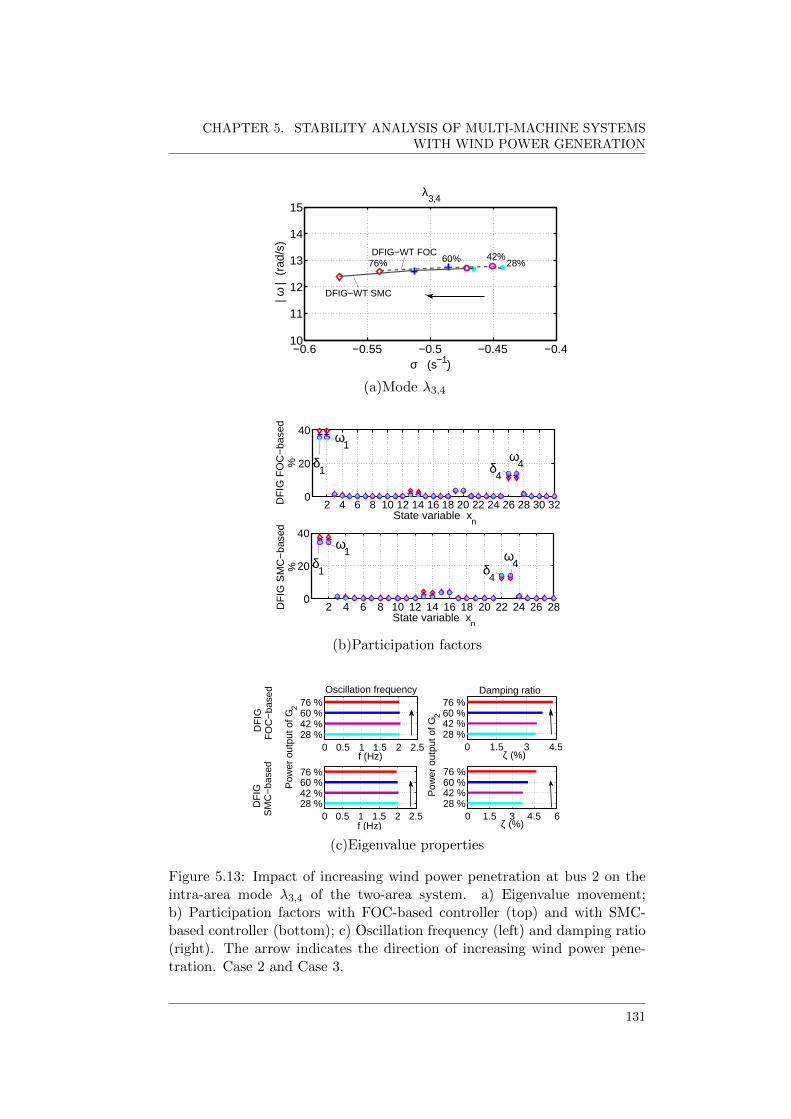
CHAPTER 5. STABILITY ANALYSIS OF MULTI-MACHINE SYSTEMSWITH WIND POWER GENERATION
−0.6 −0.55 −0.5 −0.45 −0.410
11
12
13
14
15
σ (s−1)
| ω |
(ra
d/s)
λ3,4
42%28%60%76%
DFIG−WT FOC
DFIG−WT SMC
(a)Mode λ3,4
2 4 6 8 10 12 14 16 18 20 22 24 26 28 30 320
20
40
DF
IG F
OC
−ba
sed
%
State variable xn
2 4 6 8 10 12 14 16 18 20 22 24 26 280
20
40
State variable xn
DF
IG S
MC
−ba
sed
% δ1
δ1
ω1
ω1
ω4δ
4
ω4δ
4
(b)Participation factors
0 0.5 1 1.5 2 2.528 %42 %60 %76 %
f (Hz)
Oscillation frequency
DF
IG
FO
C−
base
d
P
ower
out
put o
f G2
0 1.5 3 4.528 %42 %60 %76 %
ζ (%)
Pow
er o
utpu
t of G
2
Damping ratio
0 1.5 3 4.5 628 %42 %60 %76 %
ζ (%)0 0.5 1 1.5 2 2.5
28 %42 %60 %76 %
f (Hz)
DF
IG
S
MC
−ba
sed
(c)Eigenvalue properties
Figure 5.13: Impact of increasing wind power penetration at bus 2 on theintra-area mode λ3,4 of the two-area system. a) Eigenvalue movement;b) Participation factors with FOC-based controller (top) and with SMC-based controller (bottom); c) Oscillation frequency (left) and damping ratio(right). The arrow indicates the direction of increasing wind power pene-tration. Case 2 and Case 3.
131

5.3. THE TWO-AREA SYSTEM
−0.6 −0.5 −0.4 −0.3 −0.2 −0.10
1
2
3
4
5
σ (s−1)
| ω |
(ra
d/s)
λ5,6
76%60%
42%
28%28%42%
60%76%
DFIG−WT SMC
DFIG−WT FOC
(a)Mode λ5,6
2 4 6 8 10 12 14 16 18 20 22 24 26 28 30 320
20
40
DF
IG F
OC
−ba
sed
%
State variable xn
2 4 6 8 10 12 14 16 18 20 22 24 26 280
20
40
State variable xn
DF
IG S
MC
−ba
sed
%
δ1
ω1
δ1
ω1
ωt
θωt
δ3
ω3
δ4
ω4
θωt
ωt
ω3δ
3 δ4
ω4
(b)Participation factors
0 0.2 0.4 0.628 %42 %60 %76 %
f (Hz)
Oscillation frequency
DF
IG
F
OC
−ba
sed
Pow
er o
utpu
t of G
2
0 2 4 628 %42 %60 %76 %
ζ (%)
Pow
er o
utpu
t of G
2
Damping ratio
0 0.2 0.4 0.628 %42 %60 %76 %
f (Hz)
DF
IG
S
MC
−ba
sed
0 6 12 1828 %42 %60 %76 %
ζ (%)
(c)Eigenvalue properties
Figure 5.14: Impact of increasing wind power penetration at bus 2 on theintra-area mode λ5,6 of the two-area system. a) Eigenvalue movement;b) Participation factors with FOC-based controller (top) and with SMC-based controller (bottom); c) Oscillation frequency (left) and damping ratio(right). The arrow indicates the direction of increasing wind power pene-tration. Case 2 and Case 3.
132
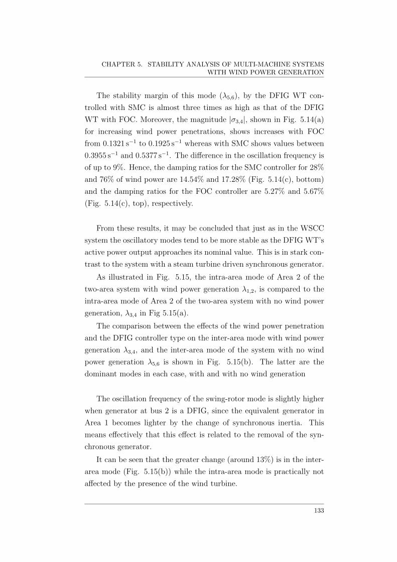
CHAPTER 5. STABILITY ANALYSIS OF MULTI-MACHINE SYSTEMSWITH WIND POWER GENERATION
The stability margin of this mode (λ5,6), by the DFIG WT con-
trolled with SMC is almost three times as high as that of the DFIG
WT with FOC. Moreover, the magnitude |σ3,4|, shown in Fig. 5.14(a)
for increasing wind power penetrations, shows increases with FOC
from 0.1321 s−1 to 0.1925 s−1 whereas with SMC shows values between
0.3955 s−1 and 0.5377 s−1. The difference in the oscillation frequency is
of up to 9%. Hence, the damping ratios for the SMC controller for 28%
and 76% of wind power are 14.54% and 17.28% (Fig. 5.14(c), bottom)
and the damping ratios for the FOC controller are 5.27% and 5.67%
(Fig. 5.14(c), top), respectively.
From these results, it may be concluded that just as in the WSCC
system the oscillatory modes tend to be more stable as the DFIG WT’s
active power output approaches its nominal value. This is in stark con-
trast to the system with a steam turbine driven synchronous generator.
As illustrated in Fig. 5.15, the intra-area mode of Area 2 of the
two-area system with wind power generation λ1,2, is compared to the
intra-area mode of Area 2 of the two-area system with no wind power
generation, λ3,4 in Fig 5.15(a).
The comparison between the effects of the wind power penetration
and the DFIG controller type on the inter-area mode with wind power
generation λ3,4, and the inter-area mode of the system with no wind
power generation λ5,6 is shown in Fig. 5.15(b). The latter are the
dominant modes in each case, with and with no wind generation
The oscillation frequency of the swing-rotor mode is slightly higher
when generator at bus 2 is a DFIG, since the equivalent generator in
Area 1 becomes lighter by the change of synchronous inertia. This
means effectively that this effect is related to the removal of the syn-
chronous generator.
It can be seen that the greater change (around 13%) is in the inter-
area mode (Fig. 5.15(b)) while the intra-area mode is practically not
affected by the presence of the wind turbine.
133

5.3. THE TWO-AREA SYSTEM
−1−0.9−0.815.515.615.7
PG2
= 28 % PG2
= 42 % PG2
= 60 % PG2
= 76 %
−0.95 −0.9 −0.85 −0.8 −0.7514
14.5
15
15.5
16
16.5
17
σ (s−1)
| ω |
(rad
/s)
Case 1All SG (λ
3,4)
Case 2DFIG−WT FOC (λ
1,2)
Case 3DFIG−WT SMC (λ
1,2)
(a)Intra-area mode of Area 2
−1−0.9−0.815.515.615.7
PG2
= 28 % PG2
= 42 % PG2
= 60 % PG2
= 76 %
−0.65 −0.6 −0.55 −0.5 −0.45 −0.4 −0.358
10
12
14
16
σ (s−1)
| ω |
(rad
/s)
Case 1All SG (λ
5,6)
Case 2DFIG−WT FOC (λ
3,4)
Case 3DFIG−WT SMC (λ
3,4)
(b)Inter-area mode
Figure 5.15: Impact of wind power penetration on (a) the intra-area modeof Area 2, and (b) the inter-area mode, compared with the base case. Thearrow indicates the direction of increasing wind power dispatch.
134
CHAPTER 5. STABILITY ANALYSIS OF MULTI-MACHINE SYSTEMSWITH WIND POWER GENERATION
It should be noticed that the inter-are mode of the test power sys-
tem with wind power penetration is not linked to the same buses as in
the base case (with no wind generation).
The damping ratio is a critical parameter in the system stability.
Thus, the obtained damping ratio for the three cases (G2 as a SG, G2
as a DFIG WT FOC and G2 as a DFIG WT SMC) can then be used
to judge the effect of DFIG control algorithms on the stability phe-
nomena. Moreover, it can directly be assessed by means of graphical
information about the eigenvalue movement.
The SMC controller case exhibits more desirable characteristics
than the FOC controller. Although the damping ratio of the SMC
controller for the inter-area mode between buses 1 and 4 (λ3,4), is only
5% better than the FOC controller, its impact on the damping of the
inter-area mode between bus 1 and the buses in the Area 2 is far mode
significant, it is about three times higher.
Moreover, the increase of wind power level contributes to enhance
the performance of the system with DFIG WT SMC, whereas the op-
erating condition does not affect the performance with FOC controller.
It is noticed that DFIG oscillations are also present in this case,
similarly to the case of a DFIG directly connected to a strong grid.
The DFIG with SMC presents a better dynamic behaviour than the
DFIG with FOC.
The behaviour of the electrical mode of the DFIG, λ7,8, is shown
in Fig. 5.16. In Fig. 5.16(a), the magnitude of the DFIG with SMC
exhibits values twice as larger as the DFIG with FOC. The magnitudes
|σ9,10| in Case 2 are 10.17 s−1, 14.19 s−1, 19.59 s−1 and, 23.77 s−1 while
in Case 3 are: 24.39 s−1, 30.52 s−1, 38.34 s−1 and 44.17 s−1. These values
correspond to increases in wind power generation of 28%, 42%, 60%
and, 76%, respectively.
135

5.3. THE TWO-AREA SYSTEM
−40 −30 −20 −10 0350
400
450
λ7,8
| ω |
(rad
/s)
σ (s−1)
42% 28%76% 60%
42%
28%
60%76%
DFIG−WT SMCDFIG−WT FOC
(a)Mode λ7,8
2 4 6 8 10 12 14 16 18 20 22 24 26 28 30 320
50
State variable xn
DF
IG F
OC
−ba
sed
%
2 4 6 8 10 12 14 16 18 20 22 24 26 280
20
40
State variable xn
DF
IG S
MC
−ba
sed
%
eSd e
Sq
eSd
eSq
iSqi
Sd
(b)Participation factors
0 25 50 7028 %42 %60 %76 %
f (Hz)
DF
IG
FO
C−
base
d
Pow
er o
utpu
t of G
2
Oscillation frequency
0 20 40 60 8028 %42 %60 %76 %
f (Hz)
DF
IG
SM
C−
base
d
0 2 4 6 828 %42 %60 %76 %
ζ (%)
Pow
er o
utpu
t of G
2
Damping ratio
0 2 4 6 8 10 1228 %42 %60 %76 %
ζ (%)
(c)Eigenvalue properties
Figure 5.16: Impact of increasing wind power penetration at bus 2 on theintra-area mode λ7,8 of the two-area system. a) Eigenvalue movement;b) Participation factors with FOC-based controller (top) and with SMC-based controller (bottom); c) Oscillation frequency (left) and damping ratio(right). The arrow indicates the direction of increasing wind power pene-tration. Case 2 and Case 3.
136

CHAPTER 5. STABILITY ANALYSIS OF MULTI-MACHINE SYSTEMSWITH WIND POWER GENERATION
This is a high frequency oscillatory mode near the grid frequency,
Fig. 5.16(c), left.
As shown in Fig. 5.16(c), right, the damping is higher using the
SMC-based strategy (bottom plot).
When the DFIG supplies power operating above synchronous speed
(for instance 76% of P ), the damping of the electrical mode by SMC
control is 10.7% in contrast to the 6.5% offered by the FOC control.
The behaviour of the mechanical mode of the DFIG, λ9,10, is shown
in Fig. 5.17. Similarly to the case of the electrical mode, the magnitude
of the mechanical oscillation with the DFIG under SMC-based control
scheme also exhibits values twice as large as than those under FOC, as
shown in Fig. 5.17(a); while |σ7,8| has values of around 4 s−1, in Case
3 and it has values of around 1.8 s−1 in Case 2.
This mode oscillates with a frequency of around 1.6 Hz, Fig.5.17(c),
LHS plot. As shown in Fig. 5.17(c), RHS plot, the damping is higher
with SMC, bottom plot. Despite the fact that this is a well damped
out mode (> 15%), the damping of the electrical mode by SMC control
is about 37% compared to the 17% offered by the FOC control.
The damping of the mechanical mode remains almost with no change
in the face of DFIG WT power generation changes.
Therefore, the stability margins afforded by SMC to both electrical
and mechanical modes, is about double the stability margins offered
by FOC.
These results show quite amply that the SMC controller exhibits
a superior performance over the FOC controller. Hence,power system
stability may be improved through a wider deployment of the DFIG
SMC wind technology.
137

5.3. THE TWO-AREA SYSTEM
−4.5 −4 −3.5 −3 −2.5 −2 −1.59.5
10
10.5
11
σ (s−1)
λ9,10
| ω |
(rad
/s) 76%
60%
42%
28%DFIG−WT SMC
DFIG−WT FOC
(a) Mode λ9,10
2 2 4 6 8 10 12 14 16 18 20 22 24 26 28 30 320
50
100
State variable xn
DF
IG F
OC
−ba
sed
%
2 4 6 8 10 12 14 16 18 20 22 24 26 280
50
100
State variable xn
DF
IG S
MC
−ba
sed
%
ωR
ωR θωt
θωt
(b) Participation factors
0 0.5 1 1.5 228 %42 %60 %76 %
f (Hz)
DF
IG
FO
C−
base
d
Pow
er o
utpu
t of G
2
Oscillation frequency
0 5 10 15 2028 %42 %60 %76 %
ζ (%)
Damping ratio
Pow
er o
utpu
t of G
2
0 10 20 30 4028 %42 %60 %76 %
ζ (%)0 0.5 1 1.5 2
28 %42 %60 %76 %
f (Hz)
DF
IG
SM
C−
base
d
(c) Eigenvalue properties
Figure 5.17: Impact of increasing wind power penetration at bus 2 on theintra-area mode λ9,10 of the two-area system. a) Eigenvalue movement;b) Participation factors with FOC-based controller (top) and with SMC-based controller (bottom); c) Oscillation frequency (left) and damping ratio(right). The arrow indicates the direction of increasing wind power pene-tration. Case 2 and Case 3.
138
E~liillJ±J U±l±LI~illJE±l
§D §E
~§

CHAPTER 5. STABILITY ANALYSIS OF MULTI-MACHINE SYSTEMSWITH WIND POWER GENERATION
5.4 Conclusions
The impact of the integration of wind power generation systems with
double-fed induction generators has been assessed in this chapter. The
advantage of using this variable-speed wind turbine concept in mixed
generation to improve on the stability of power networks has been
demonstrated under different test case scenarios, by computer simula-
tion.
Field Oriented Control and Sliding Mode Control strategies have
been used to elucidate on the contribution that wind generator con-
trollers may exert on network damping. The analytical validation
illustrates the effectiveness and potential capability of the proposed
Sliding Mode Control approach to provide a dynamic enhancement of
the DFIG itself, and to achieve a much superior performance of grid
connected wind turbines.
139

5.4. CONCLUSIONS
140

Chapter 6
Transient Stability
This chapter addresses the issue of transient stability assessment of
wind power generators with particular reference to power system os-
cillations damping. A control system based on Sliding Mode Control
principles is investigated in DFIG WT systems to contribute to network
operational support. Simulation results are provided and discussed to
show the potential of the nonlinear controller to enhance damping of
inter-area oscillations.
6.1 Background
It should be remarked that many important contributions have been
made toward the understanding of dynamic interactions between con-
ventional generation and wind power generation, by resorting to tran-
sient stability models and methods and linearized models suitable for
modal analyses.
In early works [90], the dynamic and transient stability properties of
wind turbine generators integrated into power systems were explored.
The study was addressed considering both, single and grouped wind
turbines and the influence of electrical and wind speed disturbances.
Further studies to understand the dynamic characteristics of electri-
cal network comprising wind energy generation can also be found in
[52],[111].
141

6.1. BACKGROUND
Determining the impact of DFIG generation on large-scale power
system stability has been a major concern for quite some time, includ-
ing among others things, the dynamic response to short-circuit faults
and system perturbations due to synchronous generators and transmis-
sion line outages, damping of oscillations, etc.
It has been reported in the open literature that DFIG WT have
the capacity to augment the transient stability margin of conventional
synchronous generators when integrated in the same electrical network
[100, 131, 132]. One of the reasons given is that the DFIG’s two rotor
current regulators also act upon the other generators in the vicinity,
improving their dynamic behaviour. Moreover, DFIG deployment re-
duces the dynamic reactive compensation demands on both neighbour-
ing generators and the power network, which would reduce instances
of voltage collapses in the power network.
In [132], simulation studies carried out with and with no wind power
integrated into the power grid, showed that in cases of severe grid faults
the fast control schemes of the DFIG converters do help to ride through
the fault and to maintain the integrity of the whole system. It was also
pointed out that a DFIG WT does not suffer problems of angular sta-
bility, as it is the case with conventional synchronous generators and
that DFIG WT integration makes up for an improved transient perfor-
mance of the system.
A great deal of very useful conclusions have been drawn by com-
paring the transient stability margins of power networks with variable-
speed wind system and those of power networks with fixed speed wind
systems. Attention has been drawn to the inherent risk that fixed speed
wind turbines have of undergoing voltage and rotor speed instability,
initiated by a short-circuit fault or by the tripping of a synchronous
generator and a key conclusion has been that that risk is much lower
with variable speed wind turbines [133].
142

CHAPTER 6. TRANSIENT STABILITY
The impact of DFIG WT on weak transmission systems was inves-
tigated in [56], where the results showed that DFIGs yield an improved
damping performance compared to conventional synchronous genera-
tors of equivalent ratings, a study carried out for various wind plant
load factors and covering a range of dynamic response of the turbines
to short-circuit faults. It is recommended in [134] that transient simu-
lation studies be carried out to assess the post-disturbance behaviour
of a power system for a range of credible operating scenarios and dis-
turbances, even if the system eigenvalues have been determined and
showed the system to be stable.
The impact of short-circuit faults, load disturbances and voltage
dips on the dynamic performance of DFIG WTs has also been ad-
dressed in [135, 136, 119]. It was found in [135] that the dynamic
behaviour of a DFIG subjected to a voltage dip is dominated by the
stator dynamics with poorly damped modes. These, in turn, are greatly
affected by the rotor current control bandwidth and active damping,
rotor back-emf voltages and DFIG power factor. In [136] a new con-
trol scheme was put forward in order to provide the DFIG WT with a
much improved voltage control and voltage recovery following a fault.
Furthermore, the authors claim that the new control scheme give the
DFIG WT the capacity to withstand fault clearances over synchronous
generator with conventional excitation control, for an ample margin.
At the modelling and simulation level, a major disadvantage of the
DFIG WT has been the relative complexity and computing demands
of its mathematical model, which hinders the transient analysis of the
system and limits the simulations studies of whole wind generation
system. Great many research efforts have been made to overcome this
outstanding issue. In order to reduce simulation times and the power
system model complexity, DFIG-based wind turbine models compatible
with transient analysis programs have been developed and published in
the open literature [110, 137, 138]. By way of example, in [110] a sim-
143

6.1. BACKGROUND
plified DFIG WT model was developed where the power converter is
represented by an equivalent voltage source, which regulates the rotor
current to meet the scheduled active and reactive power production.
The model performance was tested by simulating the interaction be-
tween the Arklow Bank Wind Farm and the Irish National Grid. The
proposed model is computationally efficient and suitable for large scale
power system analysis but owing to the intrinsic assumption made in
the model, it cannot be used to study the internal dynamic perfor-
mance of the power converter.
The authors in [137] published a simplified model of the DFIG,
alternative to the third-order model, which renders a more intuitive
estimation of the DFIG performance under transient conditions. The
model yields explicit information of the active and reactive power in-
jections through the stator, as well as balance and unbalanced voltage
drops due to grid faults. The model reproduces the behaviour of the
DFIG by resorting to two second-order transfer functions. The work
at [138], puts forward yet another alternative, it uses selective modal
analysis to reduce the wind turbine model for time domain simulations
by focusing on the most relevant modes and variables. The model was
applied in two test systems and it showed to match closely the be-
haviour of the original power system, in cases of transmission lines and
synchronous generators outages.
The impact of reduced inertia (due to increased wind power pene-
tration) on transient stability performance has been also examined. It
has been found that the transient performance is negatively affected by
certain disturbances, which nevertheless may be ameliorated by control
to overcome the decoupling of the inertia in DFIGs.
It has been discussed in Chapter 2, that various mechanisms are
available to provide the DFIG with frequency response capability; for
instance, primary frequency control based on grid frequency deviation
144

CHAPTER 6. TRANSIENT STABILITY
[19], frequency response by unloading the wind turbine [20, 72], sup-
plementary control similar to the natural inertial response [67], etc.
The authors in [121], assessed the impact of increased DFIG pen-
etration on transient stability through the excitation of the dominant
modes, by applying specific faults at buses close to the generators with
the largest participation factors. Both detrimental and beneficial ef-
fects of increased DFIG penetration on the system were identified by
applying this technique covering a range of fault scenarios.
6.2 DFIG dynamic model
In a double-fed induction generator the wound rotor is fed through
a variable frequency converter via the slip rings which are attached
to the rotor circuit. The rotor converter is commonly referred to as
the machine side converter (MSC). The stator windings are directly
connected to the grid. This arrangement is schematically depicted in
Fig. 6.1.
VS
VR
dc
Rotor
Side
Converter
Grid
Side
Converter
Figure 6.1: Converter configuration for the DFIG-based wind turbine
145

6.3. DFIG CONTROL DESIGN
6.2.1 Dynamic equations of the machine
In this study the DFIG is represented by a balanced continuous-time
model by replacing the flux-currents relations in equations (3.70)-(3.73).
This yields the following dq axis equations expressed in per unit,
vSdq= −RSiSdq
− LSωelB
diSdq
dt− LoωelB
diRdq
dt+ jωSLSiSdq
+ jωSLoiRdq
(6.1)
vRdq= −RRiRdq
− LoωelB
diSdq
dt− LRωelB
diRdq
dt+ jsωSLoiSdq
+ jsωSLRiRdq
(6.2)
where ωelB, is the electrical base speed, s = 1 − ωRωS
, is the slip fre-
quency, and ωR, is the rotor speed.
6.3 DFIG Control Design
6.3.1 Sliding Control Design in the Machine Side
Converter
From equations (6.1)-(6.2), the rotor voltage at the machine side con-
verter terminals can be obtained as follows:
(vSdq
vRdq
)= − 1
ωelB
(LS Lo
Lo LR
)d
dt
(iSdq
iRdq
)+
(−RS + jLS jωSLo
jsωSLo −RR + jsωSLR
)(iSdq
iRdq
)
Solving for the current derivatives,
d
dt
(iSdq
iRdq
)=
ωelB
σLRLS
(LR −Lo
−Lo LS
)(−RS + jLS jωSLo
jsωSLo −RR + jsωSLR
)(iSdq
iRdq
)− . . .
. . .− ωelB
σLRLS
(LR −Lo
−Lo LS
)(vSdq
vRdq
)
146

CHAPTER 6. TRANSIENT STABILITY
with σ = 1− L2o
LSLR
d
dt
(iSdq
iRdq
)=
ωelB
σLSLR
LR (−RS + jLS)− LojsωSLo −jωSLRLo − Lo (−RR + jsωSLR)
−Lo (−RS + jLS) + LSsωSjLo −jωSLoLo + LS (−RR + jsωSLR)
. . .
. . .
(iSdq
iRdq
)+
ωelB
σLSLR
(LR −Lo
−Lo LS
)(vSdq
vRdq
)
Developing further this equations and separating imaginary and real
terms, yields,
d
dt
(iSd
+ jiSq
iRd+ jiRq
)=
ωelB
σLSLR
(−RSLR + j
(LSLR − L2
osωS
)LoRR + jLRLoωS (1− s)
LoRS − jLoLS (1− sωS) −RRLS + jωS
(LSLRs− L2
o
)) . . .
. . .
(iSd
+ jiSq
iRd+ jiRq
)+
ωelB
σLSLR
(LR −Lo
−Lo LS
)(vSd
+ jvSq
vRd+ jvRq
)
d
dt
iSd
iSq
iRd
iRq
=ωelB
σLSLR
Ksr,1
iSd
iSq
iRd
iRq
+
LR 0 −Lo 0
0 LR 0 −Lo
−Lo 0 LS 0
0 −Lo 0 LS
vSd
vSq
vRd
vRq
with
Ksr,1 =
−RSLR −LSLR + L2
osωS LoRR LRLoωS (1− s)LSLR − L2
osωS −RSLR LRLoωS (1− s) LoRR
LoRS −LoLS (1− sωS) −RRLS −ωS
(LSLRs− L2
o
)LoLS (1− sωS) LoRS ωS
(LSLRs− L2
o
)−RRLS
This expression may be expressed in a more general form;
d
dtx = Ax + Bu = Ax + BSuS + BRuR (6.3)
with
A =ωelB
σLSLRKsr,1, BS =
ωelB
σLSLR
LR 0
0 LR
−Lo 0
0 −Lo
, BR =ωelB
σLSLR
−Lo 0
0 −Lo
LS 0
0 LS
147
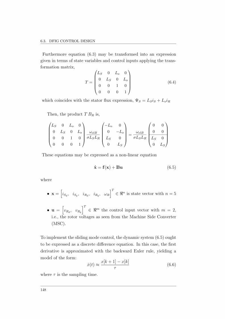
6.3. DFIG CONTROL DESIGN
Furthermore equation (6.3) may be transformed into an expression
given in terms of state variables and control inputs applying the trans-
formation matrix,
T =
LS 0 Lo 0
0 LS 0 Lo
0 0 1 0
0 0 0 1
(6.4)
which coincides with the stator flux expression, ΨS = LSiS + LoiR
Then, the product T BR is,LS 0 Lo 0
0 LS 0 Lo
0 0 1 0
0 0 0 1
ωelBσLSLR
−Lo 0
0 −LoLS 0
0 LS
=ωelBσLSLR
0 0
0 0
LS 0
0 LS
These equations may be expressed as a non-linear equation
x = f(x) + Bu (6.5)
where
• x =[iSd, iSq , iRd
, iRq , ωR
]T∈ <n is state vector with n = 5
• u =[vRd
, vRq
]T∈ <m the control input vector with m = 2,
i.e., the rotor voltages as seen from the Machine Side Converter
(MSC).
To implement the sliding mode control, the dynamic system (6.5) ought
to be expressed as a discrete difference equation. In this case, the first
derivative is approximated with the backward Euler rule, yielding a
model of the form:
x(t) ≈ x[k + 1]− x[k]
τ(6.6)
where τ is the sampling time.
148
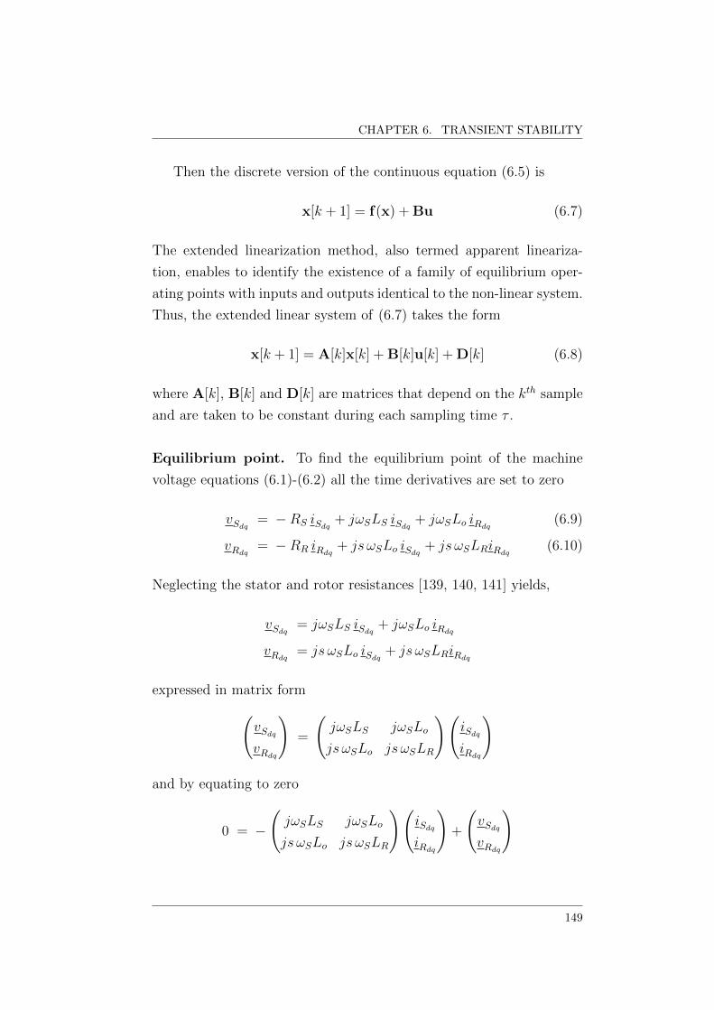
CHAPTER 6. TRANSIENT STABILITY
Then the discrete version of the continuous equation (6.5) is
x[k + 1] = f(x) + Bu (6.7)
The extended linearization method, also termed apparent lineariza-
tion, enables to identify the existence of a family of equilibrium oper-
ating points with inputs and outputs identical to the non-linear system.
Thus, the extended linear system of (6.7) takes the form
x[k + 1] = A[k]x[k] + B[k]u[k] + D[k] (6.8)
where A[k], B[k] and D[k] are matrices that depend on the kth sample
and are taken to be constant during each sampling time τ .
Equilibrium point. To find the equilibrium point of the machine
voltage equations (6.1)-(6.2) all the time derivatives are set to zero
vSdq= −RS iSdq
+ jωSLS iSdq+ jωSLo iRdq
(6.9)
vRdq= −RR iRdq
+ js ωSLo iSdq+ js ωSLRiRdq
(6.10)
Neglecting the stator and rotor resistances [139, 140, 141] yields,
vSdq= jωSLS iSdq
+ jωSLo iRdq
vRdq= js ωSLo iSdq
+ js ωSLRiRdq
expressed in matrix form(vSdq
vRdq
)=
(jωSLS jωSLo
js ωSLo js ωSLR
)(iSdq
iRdq
)
and by equating to zero
0 = −
(jωSLS jωSLo
js ωSLo js ωSLR
)(iSdq
iRdq
)+
(vSdq
vRdq
)
149

6.3. DFIG CONTROL DESIGN
and pre-multiplying by
(LR −Lo−Lo LS
)
0 =
(LR −Lo−Lo LS
)[(−jωSLS −jωSLo−js ωSLo −js ωSLR
)(iSdq
iRdq
)+
(vSdq
vRdq
)]yields
0 =
(−jωSLSLR + js ωSLoLo −jωSLRLo + js ωSLRLo
jωSLSLo − js ωSLoLS jωSL2o − js ωSLRLS
)(iSdq
iRdq
)+ . . .
. . .+
(LR −Lo−Lo LS
)(vSdq
vRdq
)
0 =
(−jωS (LRLS − sL2
o) −jωSLoLR (1− s)jLoLSωS (1− s) −jωS (sLRLS − L2
o)
)(iSd
+ jiSq
iRd+ jiRq
)+ . . .
. . .+
(LR −Lo−Lo LS
)(vSd
+ jvSq
vRd+ jvRq
)yields,
0 =Ksr,2
iSd
iSq
iRd
iRq
+
LR 0 −Lo 0
0 LR 0 −Lo−Lo 0 LS 0
0 −Lo 0 LS
vSd
vSq
vRd
vRq
where
Ksr,2 =
0 ωS
(LRLS − sL2
o
)0 ωSLoLR (1− s)
−ωS
(LRLS − sL2
o
)0 −ωSLoLR (1− s) 0
0 −ωSLoLS (1− s) 0 ωS
(sLRLS − L2
o
)ωSLoLS (1− s) 0 −ωS
(sLRLS − L2
o
)0
pre-multiplying this expression by a transformation matrix
T =
LS 0 Lo 0
0 LS 0 Lo
0 0 1 0
0 0 0 1
150

CHAPTER 6. TRANSIENT STABILITY
yields an expression which coincides with the stator flux ΨS = LSiS +
LoiR, gives the system around the equilibrium point 0
0 = A0x0 + BS0uS0 + BR0uR0 (6.11)
with
x0 =[iSd
iSq iRdiRq
]T, being the state vector
uR0 =[vRd0
vRq0
]T, being the control input vector
uS0 =[vSd0
vSq0
]T, being the stator input vector
A0, BS0, BR0, being constant matrices given by
A0 =
0 ωSLSσLSLR 0 ωSLoσLSLR
−ωSLSσLSLR 0 −ωSLoσLSLR 0
0 −ωSLoLS(1− s) 0 ωS(sLRLS − L2o)
ωSLoLS(1− s) 0 −ωS(sLRLS − L2o) 0
BS0 =
σLRLS 0
0 σLRLS
−Lo 0
0 −Lo
, BR0 =
0 0
0 0
LS 0
0 LS
Sliding Control
A controller is designed to be constrained to the sampling frequency
with the control signal changing only at sampling instances. As de-
scribed in Chapter 3 the design procedure of the controller comprises
two steps, one related to computation of the sliding surface and the
other to the establishment of the control law. The design procedure in
discrete form is described below:
151

6.3. DFIG CONTROL DESIGN
• Step 1 Computation of a sliding surface s[k] = Sx[k] with suit-
able internal dynamics. In order to find the sliding surface s[k] a
linear transformation is performed to bring the system (6.5) into
the so called regular form [6],
x1 = f1(x1, x2, t)
x2 = f2(x1, x2, t) +B2(x1, x2, t)u (6.12)
where x1 ∈ <n−m, x2 ∈ <m, and B2 is an m xm non-singular
matrix. The block x1 does not depend on control, whereas the
dimension of x2 coincides with that of the control.
For the controllable system (6.5) there exists an invertible trans-
formation Trx ∈ <n(x)n, defined as:
z = Trxx (6.13)
with Trx ∈ <n×n being the matrix of the linear transformation.
In this new state coordinates the system becomes:
z[k + 1] = A[k]z[k] + B[k]u + D[k] (6.14)
or in a more explicit form,[z1[k + 1]
z2[k + 1]
]=
[A11[k] A12[k]
A21[k] A22[k]
][z1[k]
z2[k]
]+ . . .
. . .+
[0n−m×m
B2[k]
]u[k] +
[D1[k]
D2[k]
](6.15)
where z1 ∈ <n−m and z2 ∈ <m are all matrices Aij∀i, j = 1..2,
Di∀i = 1..2 of appropriate dimensions and B2 ∈ <m×m has full
rank.
Let e[k] = z[k] − zref be the new state vector where zref is the
requested reference value. The system may be expressed in these
152

CHAPTER 6. TRANSIENT STABILITY
new coordinates as
e[k + 1] = A[k]e[k] + B[k]u+ D[k] (6.16)
where D[k] = D + (A[k]− I) zref
If the sliding mode manifold in these new coordinates is linear,
then
s[k] = Ce[k] = [ F Im×m ]
[e1[k]
e2[k]
]= Fe1[k] + e2[k] (6.17)
with F ∈ <m×n. Assuming that a controller exits that forces the
system into sliding mode (i.e. s[k] = 0), the following relationship
applies
e2[k] = −Fe1[k] (6.18)
Substituting the above equation into Eq. (6.15) yields
e1[k + 1] = (A11[k]− A12[k]F )e1[k] = Asm[k]e1[k] (6.19)
Matrix F is chosen such that Asm[k] = A11 − A12F has stable
eigenvalues and performs the desired dynamics of the closed-loop
while the system is in sliding mode.
Notice that once the system is in sliding mode the order of the
closed loop system dynamics is characterized by Eq. (6.19) whose
order is (n − m), an order that it is less than the order of the
original uncontrolled system (n).
• Step 2 Establishing a control law that steers the system towards
the sliding surface at a finite time and keeps the closed loop
dynamics confined to the manifold. To reach the sliding surface
in one sampling period, i.e. s[k + 1] = 0, the reaching law is
s[k + 1] = CA[k]e[k] + CB[k]u[k] + CD[k] = 0
153
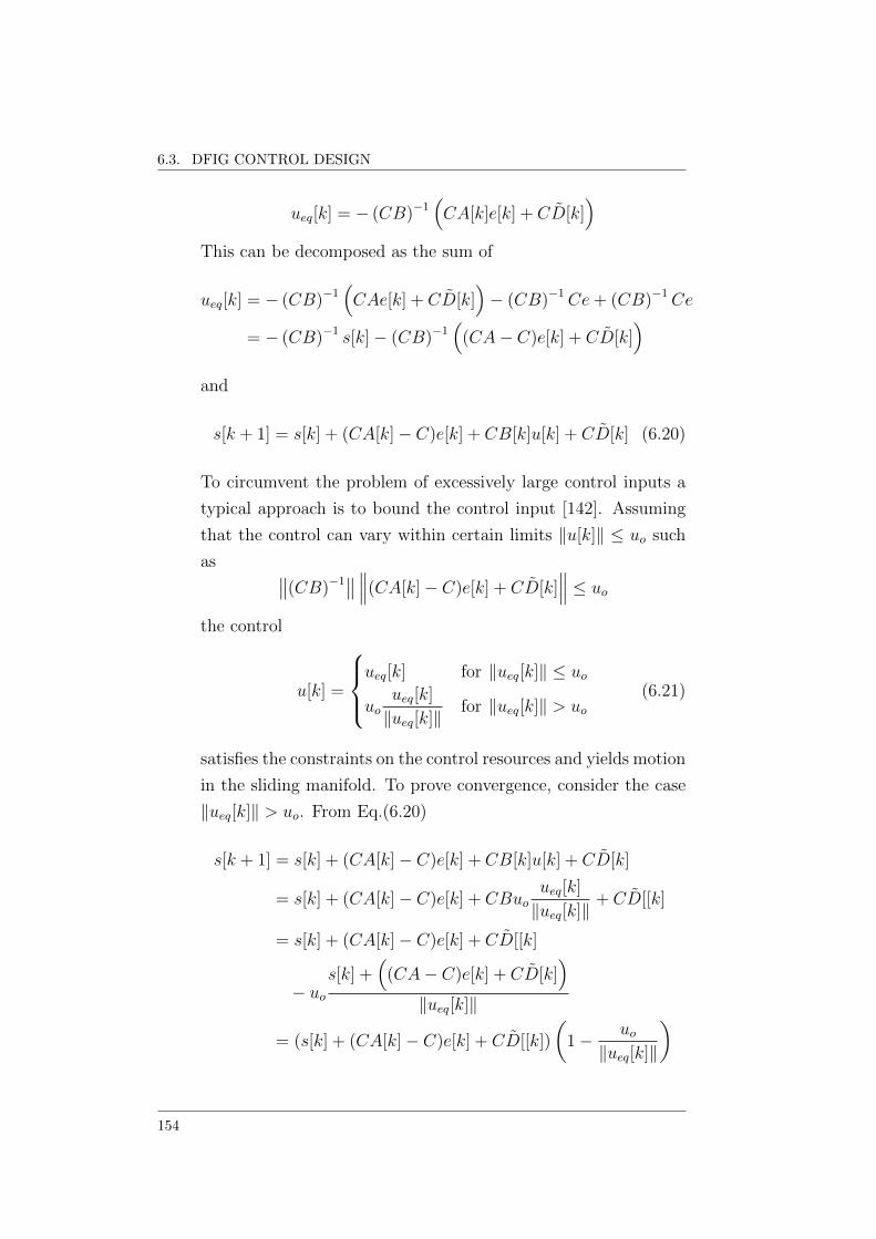
6.3. DFIG CONTROL DESIGN
ueq[k] = − (CB)−1(CA[k]e[k] + CD[k]
)This can be decomposed as the sum of
ueq[k] = − (CB)−1(CAe[k] + CD[k]
)− (CB)−1Ce+ (CB)−1Ce
= − (CB)−1 s[k]− (CB)−1(
(CA− C)e[k] + CD[k])
and
s[k + 1] = s[k] + (CA[k]− C)e[k] + CB[k]u[k] + CD[k] (6.20)
To circumvent the problem of excessively large control inputs a
typical approach is to bound the control input [142]. Assuming
that the control can vary within certain limits ‖u[k]‖ ≤ uo such
as ∥∥(CB)−1∥∥∥∥∥(CA[k]− C)e[k] + CD[k]
∥∥∥ ≤ uo
the control
u[k] =
ueq[k] for ‖ueq[k]‖ ≤ uo
uoueq[k]
‖ueq[k]‖for ‖ueq[k]‖ > uo
(6.21)
satisfies the constraints on the control resources and yields motion
in the sliding manifold. To prove convergence, consider the case
‖ueq[k]‖ > uo. From Eq.(6.20)
s[k + 1] = s[k] + (CA[k]− C)e[k] + CB[k]u[k] + CD[k]
= s[k] + (CA[k]− C)e[k] + CBuoueq[k]
‖ueq[k]‖+ CD[[k]
= s[k] + (CA[k]− C)e[k] + CD[[k]
− uos[k] +
((CA− C)e[k] + CD[k]
)‖ueq[k]‖
= (s[k] + (CA[k]− C)e[k] + CD[[k])
(1− uo‖ueq[k]‖
)
154
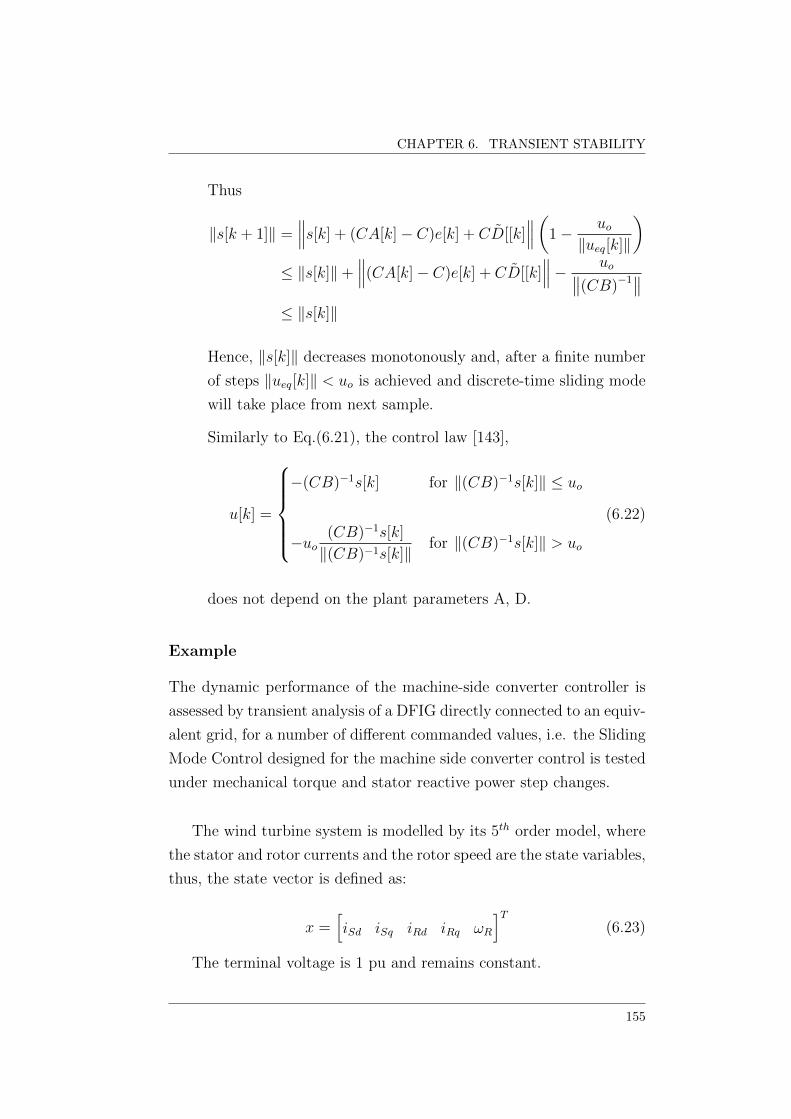
CHAPTER 6. TRANSIENT STABILITY
Thus
‖s[k + 1]‖ =∥∥∥s[k] + (CA[k]− C)e[k] + CD[[k]
∥∥∥(1− uo‖ueq[k]‖
)≤ ‖s[k]‖+
∥∥∥(CA[k]− C)e[k] + CD[[k]∥∥∥− uo∥∥(CB)−1
∥∥≤ ‖s[k]‖
Hence, ‖s[k]‖ decreases monotonously and, after a finite number
of steps ‖ueq[k]‖ < uo is achieved and discrete-time sliding mode
will take place from next sample.
Similarly to Eq.(6.21), the control law [143],
u[k] =
−(CB)−1s[k] for ‖(CB)−1s[k]‖ ≤ uo
−uo(CB)−1s[k]
‖(CB)−1s[k]‖for ‖(CB)−1s[k]‖ > uo
(6.22)
does not depend on the plant parameters A, D.
Example
The dynamic performance of the machine-side converter controller is
assessed by transient analysis of a DFIG directly connected to an equiv-
alent grid, for a number of different commanded values, i.e. the Sliding
Mode Control designed for the machine side converter control is tested
under mechanical torque and stator reactive power step changes.
The wind turbine system is modelled by its 5th order model, where
the stator and rotor currents and the rotor speed are the state variables,
thus, the state vector is defined as:
x =[iSd iSq iRd iRq ωR
]T(6.23)
The terminal voltage is 1 pu and remains constant.
155

6.3. DFIG CONTROL DESIGN
Table 6.1: DFIG-WT data
DFIG parameters
RS RR Lo LS LR H Pwrated
(pu) (pu) (pu) (pu) (pu) (s) (MW)
0.0038 0.0044 3.00 3.2250 3.2100 3.5 2
The parameters of the DFIG wind turbine system are listed in Table
6.1.
Firstly, the mechanical torque is forced to its lower value and the
wind turbine operates with zero reactive power output. Then, the me-
chanical torque is kept constant at -1 per unit whereas the reference of
reactive power is step changed.
The proposed control method provides a torque-reactive power de-
coupled control through the regulating q-axis current and d -axis cur-
rent, respectively.
• Change in the input mechanical torque:
A change in the input mechanical torque is caused by a change in
the active power output reference; with the active power output ob-
tained from the optimal power-speed curve.
Fig. 6.2 shows the simulated results where the input mechanical
torque step changed at 0.2 sec from −1 pu to −0.5 pu. It can be ob-
served that the active power is controlled by the q-axis stator and rotor
current while d -axis stator and rotor current remains constant during
the mechanical torque variation.
The output rotor voltage of the MSC, determined by SMC, is shown
in Fig. 6.3 and Fig. 6.4 depicts the control law functions of the MSC
regulator.
156

CHAPTER 6. TRANSIENT STABILITY
0 0.1 0.2 0.3 0.4 0.5−0.5
0
0.5
1
1.5i R
(pu
)
0 0.1 0.2 0.3 0.4 0.5−1.5
−1
−0.5
0
0.5
i S (
pu)
0 0.1 0.2 0.3 0.4 0.5−1.5
−1
−0.5
0
0.5
time (s)
refe
renc
es (
pu)
T
m
QS
iRd
iRq
iSd
iSq
Figure 6.2: Stator and rotor currents with Tm reference variation
0 0.1 0.2 0.3 0.4 0.5−1
−0.5
0
0.5
time (s)
v R (
pu)
vRd
vRq
Figure 6.3: Rotor voltage with Tm reference variation
157
:.._----
.~ ..
:' ... _._._ .. -
• __ . ,f
•
·
·
_ . _ . • . - J. -----'1
--- - ~-- -- ~------ -- --
•
• •
J

6.3. DFIG CONTROL DESIGN
0 0.1 0.2 0.3 0.4 0.5−0.5
0
0.5
0 0.1 0.2 0.3 0.4 0.5−0.5
0
0.5
time (s)
refe
renc
es (
pu)
u
II,P
uII,Q
uI, P
uI,Q
Figure 6.4: Control law functions with Tm reference variation
• Change in the stator reactive power reference:
A variation on the stator reactive power reference is a rather effective
mean to demonstrate the influence of the d -axis current control in mod-
ulating the reactive power output in order to enable the control of the
generator terminals.
Fig. 6.5 shows the stator and rotor currents and Fig. 6.6 shows the
voltage control at the machine terminals.
The rotor voltage output of the MSC is shown in Fig. 6.7. It can be
observed that the d -axis component of the rotor voltage varies accord-
ing to the change of reactive power and the q-axis component of the
rotor voltage remains practically constant following the reactive power
command variation.
Fig. 6.8 depicts the SMC control law functions of the MSC regula-
tor.
158
¡.... --------- ----:--- ~ -- :- - ~ -~
r

CHAPTER 6. TRANSIENT STABILITY
0 0.1 0.2 0.3 0.4 0.5−0.5
0
0.5
1
i R (
pu)
0 0.1 0.2 0.3 0.4 0.5−1
−0.5
0
0.5
i S (
pu)
0 0.1 0.2 0.3 0.4 0.5
−1
−0.5
0
0.5
time (s)
refe
renc
es (
pu)
T
m
QS
iRd
iRq
iSd
iSq
Figure 6.5: Stator and rotor currents with QS reference variation
0 0.1 0.2 0.3 0.4 0.50
0.5
1
1.5
time (s)
v S (
pu)
0 0.1 0.2 0.3 0.4 0.50
0.5
1
1.5
time (s)
e g (pu
)
vSd
vSq
egd
egq
Figure 6.6: Voltage (d-q) at generator terminals with QS reference variation
159
....................................................... ............. : ............. : .............•........... ··1 ::: [----·----r------- n
~ ~ ............ ~ ............. ; ........... ~ ............. ~ ............ .
1 ·· Jf ·· j~
~ · ... ·~~· ~ . ~ ~ - ~ ~:i -~~~~ .~ -~ · ~ ·~EJpll t· ........... ~ ............. ~ ............. , ............. : ~ .~ .. ~ .... .
.. EJ · . .
.. , ----'- '- '- '- T'- '- '--'f '- '- '-'- '-: '- '-'- '- '- : - --
.. EJ · .
.. , ----r- . - . - . - .- ~ . - . - .-- . +- .- .- . - . _:.- .-. - . - . - :. -_.
· . . . . . . . . . . . . . . . . . . . . . . . . . . . . . . . . . . . .
; . .

6.3. DFIG CONTROL DESIGN
0 0.1 0.2 0.3 0.4 0.5−1
−0.5
0
0.5
time (s)
v R (
pu)
vRd
vRq
0.1 0.2 0.3 0.4 0.5
−0.5
−0.4
−0.3
−0.2
−0.1
0
0.1
time (s)
v R (
pu)
time (s)v R (
pu)
v
Rd
vRq
Figure 6.7: Rotor voltage with QS reference variation
0 0.1 0.2 0.3 0.4 0.5−0.4
−0.3
−0.2
−0.1
0
0 0.1 0.2 0.3 0.4 0.5−0.4
−0.2
0
0.2
0.4
time (s)
refe
renc
es (
pu)
uI,P
uI,Q
uII,P
uII,Q
Figure 6.8: Control law functions with QS reference variation
160

CHAPTER 6. TRANSIENT STABILITY
6.3.2 Sliding Control Design in the Grid Side Con-
verter
The GSC is connected to the grid through a grid-side filter and it is
used to control dc-link voltage and reactive power exchange with the
grid. Fig. 6.9 shows the diagram of the back-to-back converter, where
Zf is the grid-side filter impedance, vf is the output voltage at the
grid-side converter, Eg is the grid voltage and vdc is the dc bus voltage.
Dynamic equations of the GSC
The per unit dq axis voltage equations can be written as
vfd + jvfq = egd + jegq +Rf (ifd + jifq) + Lf1
ωelB
d
dt(ifd + jifq) + . . .
. . .+ jωSLf (ifd + jifq) (6.24)
vfd = egd +Rf ifd + Lf1
ωelB
d
dtifd − ωSLf ifq (6.25)
vfq = egq +Rf ifq + Lf1
ωelB
d
dtifq + ωSLf ifd (6.26)
The stator and the rotor converters are related through the active
power balance in the dc link capacitor:
vdcCdcdvdcdt
= (−Pg − PR) (6.27)
GSC RSCZfIf
Eg
PR
vf vR
IRvdc
Figure 6.9: Diagram of the GSC for the DFIG-based wind turbine
161

6.3. DFIG CONTROL DESIGN
withPR = <vRi∗RPg = <
egi∗f
(6.28)
By aligning the d q-axis with the voltage eg such that eg = egd, and
egq = 0, the direct axis component of the grid side converter current
controls the active power trough the stator converter,
Pg = <egd (ifd − jifq) = egdifd (6.29)
thereby equation (6.27) becomes,
vdcCdcdvdcdt
= (−egdifd − PR)
and reordering the voltage and dc link capacitor equations
vfd = egd +Rf ifd + Lf1
ωelB
d
dtifd − ωSLf ifq
vfq = egq +Rf ifq + Lf1
ωelB
d
dtifq + ωSLf ifd
vdcCdcdvdcdt
= (−egdifd − PR)
gives,
d
dtifd =
ωelBLf
(vfd − egd −Rf ifd + ωSLf ifq) (6.30)
d
dtifq =
ωelBLf
(vfq − egq −Rf ifq − ωSLf ifd) (6.31)
dvdcdt
=1
Cdcvdc(−egdifd − PR) (6.32)
and in matrix form,
d
dt
ifdifqvdc
=
ωelBLf
(−egd −Rf ifd + ωSLf ifq)ωelBLf
(−egq −Rf ifq − ωSLf ifd)1
Cdcvdc(−egdifd − PR)
+
ωelBLf
0
0
vfd +
0
ωelBLf
0
vfq
(6.33)
162

CHAPTER 6. TRANSIENT STABILITY
The system equations can be written in the form
x = f (x) + g1(x)u1 + · · ·+ gm(x)um (6.34)
y1 = h1 (x)
...
ym = hm (x) (6.35)
where
y1 = h1 (x) = ifq (6.36)
y2 = h2 (x) = vdc (6.37)
Feedback Linearization
The key idea of feedback linearization is to algebraically transform the
non-linear system dynamics into fully or partly linear control problem;
then linear control techniques can be applied [144]. The basic method
for accomplishing input-output linearization is to differentiate the out-
puts yi with respect to time until the control inputs appear and then
new inputs are designed that cancel out the non-linearities.
Consider the MIMO system described by (6.34)- (6.35). It is as-
sumed that each output yi has a defined relative degree γi, which rep-
resents the times that the output is differentiated.
By using Lie’s [144, 145] derivatives the process of repeated differ-
entiation begins with
yi = Lfh(x) + Lgh(x)u (6.38)
with a Lie derivative given by Lfh =∂h
∂xf.
Lie’s derivative of order zero is denoted by Lf h and Lie’s derivatives
of higher order are given by Lif h = Lh(Li−1f h
).
163

6.3. DFIG CONTROL DESIGN
In terms of Lie derivatives the output yi has a relative degree γi
if, ∃ an integer LgiL`f ≡ 0 ∀ ` < γi − 1, ∀ 1 ≤ i ≤ m, ∀x ∈ U , and
Lgi Lγi−1f h(x) 6= 0. U ⊂ <n which is in a given neighbourhood of
the equilibrium point of the system. The system’s relative degree r, is
defined to be the sum of the relative degrees of all the output variables.
Lie’s derivative for the ith output is given by
y(ri)i = Lrif hi(x) +
m∑j=1
LgjLri−1f hi(x)uj (6.39)
assuming that ri is the smallest integer such that at least one of
the inputs appears in the ith output and with LgjLri−1f hi(x) 6= 0 for at
least one j. By taking the Lie’s derivative for each ith output, yields,y(γ1)i...
y(γmi)i
=
Lγ1f h1(x)
...
Lγmf hm(x)
+ E(x)u (6.40)
where
E(x) =
Lg1L
r1−1f h1(x) · · · LgmL
r1−1f h1(x)
.... . .
...
Lg1Lrm−1f hm(x) · · · LgmL
rm−1f hm(x)
If the decoupling matrix E(x) is invertible, then the input transfor-
mation
u = E(x)−1
v1 − Lγ1f h1(x)
...
vm − Lγmf hm(x)
(6.41)
yields the decoupled dynamics
y(γi)i = vi (6.42)
The output variables of the GSC aimed at achieving a reactive
power control in order to maintain the dc voltage constant are given
by (6.36)-(6.37).
164

CHAPTER 6. TRANSIENT STABILITY
Differentiation of the output y1 with respect to time reveals a rela-
tive degree of one
y1 =ωelBLf
(−egq −Rf ifq − ωSLf ifd) +ωelBLf
vfq (6.43)
Now, differentiation of the output y2 with respect to time twice
(ri = 2), yields,
y2 =ωelBCdcvdc
(−egdifd − PR) (6.44)
y2 =ωelBCdcvdc
(−egd
ω
Lf(−egd −Rf ifd + ωSLf ifq + vfd)− PR
)− . . .
. . .− ωelBCdcv2dc
ωelBCdcvdc
(−egdifd − PR)(−egdifd − PR) (6.45)
Hence, the whole system has a relative degree of three.
These equations may be expressed in compact form as(y1
y2
)= α + β
(vfd
vfq
)(6.46)
where
α =
−ωelBLf
vfqss
ωelBCdcvdc
(ωelBLf
egdvfdss − PR)−Kdc(−egdifd − PR)2
β =
0ωelBLf
−egdω2elB
LfCdcvdc0
with
vfqss = egq +Rf ifq + ωSLf ifd,
vfdss = egd +Rf ifd − ωSLf ifq,
Kdc =ω2elB
C2dcv
3dc
165

6.3. DFIG CONTROL DESIGN
Thereafter, equation (6.46) can be rewritten as:(v1
v2
)= α + β
(vfd
vfq
)(6.47)
and the following linear form results:(y1
y2
)=
(v1
v2
)(6.48)
Since β is non-singular (except for −egdω3elB
L2fCdcvdc
= 0) in the oper-
ating range of vdc and egd, the control law can be computed as follows(vfd
vfq
)= β−1
((v1
v2
)− α
)(6.49)
Sliding Control
To design two sliding control for the equation (6.48), two decoupled
controllers for each variable (y1, y2) are realized as follows:
• Reactive current controller of the GSC:
The output reactive current is defined as (6.36) by
y1 = v1
Using the Euler’s discretization, gives the first derivative
x(t) ≈ x[k + 1]− x[k]
τ
where τ is the sampling time, yields
y11,k+1 = y11,k + τv1,k (6.50)
166

CHAPTER 6. TRANSIENT STABILITY
Defining the following sequence of maps
ω0,k = y11,k − yrefk
ω1,k = ω0,k+1 = y11,k+1 − yrefk+1
= y11,k + τv1,k − yrefk+1 (6.51)
which clearly expresses the dependence of the output variable y1 at
time k + 1 on the state x(k) and the input sequence u(k), u(k + 1).
The inverse transformation is given by,
y11,k = ω0,k + yrefk (6.52)
then the transformed system is,
ω0,k+1 = ω1,k
= ω0,k + τv1,k + yrefk − yrefk+1 (6.53)
It should be remarked that when the inputs and the initial state
of (6.53) are properly set, the various components of the state of this
system reproduce the output of the system and its next value,
v1,k = uk+1
ω0,k = yk (6.54)
then
ω1,k = yk+1 (6.55)
As the system model is described in controllable canonical form
then a function,
sk = α0ω0,k + α1ω1,k + . . .+ αn−2ωn−2,k + ωn−1,k (6.56)
with the coefficients chosen in such a manner that the polynomial
p(λ) = λn−1 + αn−2λn−2 + . . .+ α0 (6.57)
167

6.3. DFIG CONTROL DESIGN
in the complex variables λ, is Hurwitz, defines a sliding surface as,
sk = ω0,k (6.58)
and a control u such that a sliding mode occurs on sk = 0
ω0,k = 0
which define the equilibrium point y11,k→∞ = yref .
In the next instant of time the sliding mode is:
sk+1 = 0
then
sk+1 = ω0,k+1 = 0
Incorporating this restriction in (6.53)
ω0,k + τv1,k + yrefk − yrefk+1 = 0
so that the control variable becomes,
v1,k =1
τ
(−ω0,k − yrefk + yrefk+1
)v1,k =
1
τ
(−y11,k + yrefk+1
)(6.59)
It should be emphasized that the reactive current control depends
only on the reference value in the next instant of time yrefk+1, and the
reactive current measurement in the current instant of time y11,k
• dc voltage controller in the GSC:
To keep the dc voltage constant in (6.48), the second output y2 is
to be used
y2 = v2
168
CHAPTER 6. TRANSIENT STABILITY
Representing the output function y2 in controllable canonical form
[146]
y21 = y2
y21 = y2 = y22
which may be written in matrix form,(y21
y22
)=
(0 1
0 0
)(y21
y22
)+
(0
1
)v2 (6.60)
In the same way that it was done for the output y1, a discrete-time
frame will be followed: Let us consider the Euler’s discretization of the
first derivative
x(t) ≈ x[k + 1]− x[k]
τ
where τ is the sampling time.
y21,k+1 = y21,k + τy22,k
y22,k+1 = y22,k + τv2,k (6.61)
In order to transform the system into the generalized observability
canonical form (GOBCF) [147], the following sequence of maps are
defined
ω0,k = y21,k − yrefk
ω1,k = ω0,k+1 = y21,k+1 − yrefk+1
= y21,k + τy22,k − yrefk+1
ω2,k = ω1,k+1 = y21,k+1 + τy22,k+1 − yrefk+2
= y21,k + 2τy22,k + τ 2v2,k − yrefk+2 (6.62)
with the inverse transformation given by
y21,k = ω0,k + yrefk
y22,k = τ−1ω1,k − τ−1ω0,k − τ−1yrefk + τ−1yrefk+1 (6.63)
169

6.3. DFIG CONTROL DESIGN
The transformed system then reads
ω0,k+1 = ω1,k
= ω0,k + yrefk + . . .
. . .+ 2τ(τ−1ω1,k − τ−1ω0,k − τ−1yrefk + τ−1yrefk+1
)+ . . .
. . .+ τ 2v2,k − yrefk+2
= −ω0,k + 2ω1,k + τ 2v2,k − yrefk + 2yrefk+1 − yrefk+2 (6.64)
As aforementioned in the case of y1 it should be clear that if
v2,k = uk+1
ω0,k = yk (6.65)
then
ω1,k = yk+1 (6.66)
The sliding surface, defined by function (6.56), may be expressed
in terms of the transformed coordinates
sk = αoω0,k + ω1,k (6.67)
Incorporating the sliding condition sk = 0, gives
0 = αoω0,k + ω1,k = αoω0,k + ω0,k+1
or
ω0,k+1 + αoω0,k = 0
which is stable at the equilibrium point ω0,k→∞ = 0; that is,
y21,k→∞ = yref
170

CHAPTER 6. TRANSIENT STABILITY
In the next instant of time, the sliding motion is required to stay
at the equilibrium point, which means
sk+1 = 0
then
sk+1 = αoω0,k+1 + ω1,k+1 = 0
Incorporating this restriction in (6.53)
αoω1,k +(−ω0,k + 2ω1,k + τ 2v2,k − yrefk + 2yrefk+1 − y
refk+2
)= 0
the control for vdc is given by
v2,k =1
τ 2
(ω0,k − (αo − 2)ω1,k + yrefk − 2yrefk+1 + yrefk+2
)where
ω0,k = y21,k − yrefk
ω1,k = ω0,k+1 = y21,k + τy22,k − yrefk+1
ω2,k = ω1,k+1 = y21,k + 2τy22,k + τ 2v2,k − yrefk+2
Hence,
v2,k =1
τ2
(y21,k − yrefk − (αo − 2) (y21,k + τy22,k − yrefk+1) + yrefk
)− . . .
. . .− 1
τ2
(2yrefk+1 + yrefk+2
)(6.68)
If measurements of vdc,k, egd,k, ifd,k, PR,k are available, then the
value of y21,k and y22,k can be obtained from
y21,k = vdc,k (6.69)
y22,k =ω
Cdcvdc,k(−egd,kifd,k − PR,k) (6.70)
Alternatively, these quantities can be estimated by using an observer.
171
6.3. DFIG CONTROL DESIGN
With the values of v1,k,v2,k given by (6.59),(6.68), the values of vfd,
vfq according to (6.49) are obtained.
Notice that, if the control voltage of the converter is limited to a
maximum value ulim, it should verified that
‖uk,eq‖ =
∥∥∥∥∥(vfd
vfq
)∥∥∥∥∥ < ulim
Otherwise, the control signal should be limited to a maximum value
according to the expression:
uk =
uk,eq for ‖uk,eq‖ ≤ ulim
ulimuk,eq‖uk,eq‖
for ‖uk,eq‖ > ulim
Example
In this section, the transient response of the GSC control is assessed in
connection with voltage and current set point step changes. The wind
turbine is represented by a generic model which incorporates features
of wind turbine electrical controls relevant to transient stability studies.
Simulations of the grid side converter were carried out with the
following parameters:
- The filter parameters: Lf = 0.2, Rf = 0.002, Cdc = 3.5
- For the proposed controller, the design parameter αo = 0.9 and
the sampling interval was chosen to be τ = 0.1ms
- The dc voltage and reactive power references are vrefdc = 2.1,
QGSC = 0.3
The control performance is shown in Figs. 6.10 - 6.14. It is observed
in Figs. 6.10 and 6.11 that dc voltage and reactive current at the stator
side of the DFIG match rather well their respective reference signals.
172

CHAPTER 6. TRANSIENT STABILITY
0.45 0.5 0.55 0.6 0.651.95
2
2.05
2.1
time (s)
v dc (
pu)
v
dcref
vdc
0.45 0.5 0.55 0.6 0.65−1
0
1x 10
−3
i fq (
pu)
ifqref
ifq
Figure 6.10: udc control in the GSC
0.89 0.895 0.9 0.905 0.91 0.915 0.921.999
1.9995
2
2.0005
2.001
time [s]
v dc (
pu)
v
dcref
vdc
0.89 0.895 0.9 0.905 0.91 0.915 0.920
0.1
0.2
0.3
0.4
i fq (
pu)
ifqref
ifq
Figure 6.11: ifq response to a change in the reactive current of the GSC
173
, : ---. ~
. . . . . . . . . . . . . . . .. . ............... .................,. .
• • • •
.... ~--~
•
........ ---
•

6.3. DFIG CONTROL DESIGN
Fig. 6.12 depicts the dq axis components of the output voltage at
the GSC. On the other hand, if the rotor active power is varied, i.e.,
disturbed, the GSC control acts to maintain the dc-link voltage at the
specified voltage level, as shown Fig. 6.13.
0.4 0.5 0.6 0.7 0.8 0.9
0.9
1
1.1
time (s)
v fd (
pu)
0.4 0.5 0.6 0.7 0.8 0.9
−0.1−0.05
00.050.1
v fq (
pu)
Figure 6.12: Control variable d-q
0.95 1 1.05 1.11.999
2
2.001
time (s)
v dc (
pu)
v
dcref
vdc
0.95 1 1.05 1.10
0.2
0.4
time (s)
i fq (
pu)
ifqref
ifq
0.95 1 1.05 1.10
0.2
0.4
time (s)
PR (
pu)
Figure 6.13: Response to a change in the active power flow from the MSC.
174
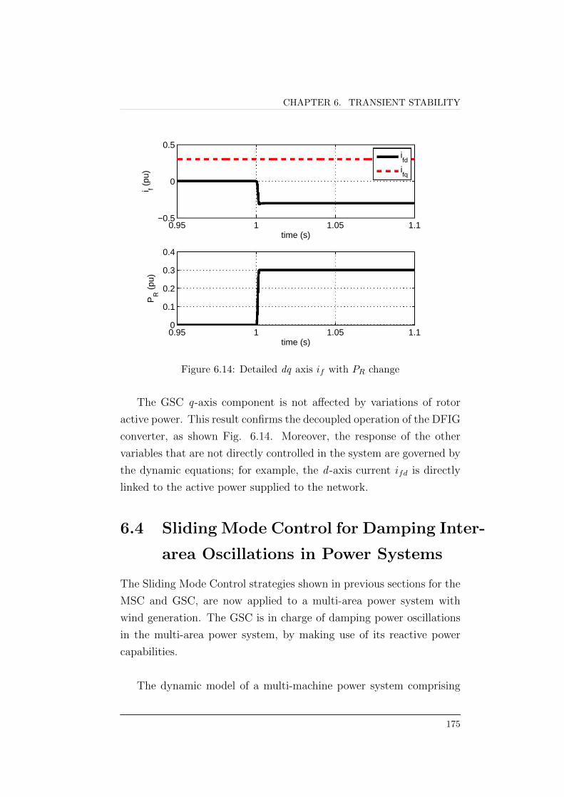
CHAPTER 6. TRANSIENT STABILITY
0.95 1 1.05 1.1−0.5
0
0.5
time (s)
i f (pu
)
ifd
ifq
0.95 1 1.05 1.10
0.1
0.2
0.3
0.4
time (s)
PR (
pu)
Figure 6.14: Detailed dq axis if with PR change
The GSC q-axis component is not affected by variations of rotor
active power. This result confirms the decoupled operation of the DFIG
converter, as shown Fig. 6.14. Moreover, the response of the other
variables that are not directly controlled in the system are governed by
the dynamic equations; for example, the d -axis current ifd is directly
linked to the active power supplied to the network.
6.4 Sliding Mode Control for Damping Inter-
area Oscillations in Power Systems
The Sliding Mode Control strategies shown in previous sections for the
MSC and GSC, are now applied to a multi-area power system with
wind generation. The GSC is in charge of damping power oscillations
in the multi-area power system, by making use of its reactive power
capabilities.
The dynamic model of a multi-machine power system comprising
175
r- - - - - - - - ~ - - - - - - - -:- - - -,
•

6.4. SLIDING MODE CONTROL FOR DAMPING INTER-AREAOSCILLATIONS IN POWER SYSTEMS
N machines may be described by the classical swing equation [21, 148,
149, 150]
δi = ωi − ω0
ωi =1
2Hi
(−Di
(ωi − ω0
)+ Pmi − Pei
)(6.71)
for i = 1, . . . , N
where the state variables δi, ωi are the relative generator power an-
gle and the relative rotor speed of machine i, respectively. Hi is the
inertia constant, Di is the per unit damping constant, ω0 is the sys-
tem speed, Pmi is the mechanical input power, and Pei is the electrical
power.
A power network comprising two dynamic areas and one wind farm
is depicted in Fig. 6.15. The transmission power network can be ex-
pressed as an admittance matrix Y of size (N + m, N + m) where N
is the number of generator buses and m is the number of wind farms
with reactive current injection capability, as schematically shown in
Fig. 6.16. The power network is taken to have L load buses.
2
Area 2Area 2
1
3
Area 1Area 1
Figure 6.15: Two areas system with wind power generation
176
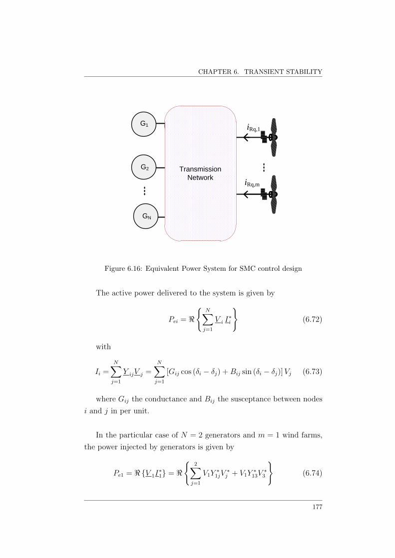
CHAPTER 6. TRANSIENT STABILITY
G1
G2
GN
Transmission
Network
iRq,1
iRq,m
G1
Figure 6.16: Equivalent Power System for SMC control design
The active power delivered to the system is given by
Pei = <
N∑j=1
V i I∗i
(6.72)
with
Ii =N∑j=1
Y ijV j =N∑j=1
[Gij cos (δi − δj) +Bij sin (δi − δj)]Vj (6.73)
where Gij the conductance and Bij the susceptance between nodes
i and j in per unit.
In the particular case of N = 2 generators and m = 1 wind farms,
the power injected by generators is given by
Pe1 = <V 1I∗1 = <
2∑j=1
V1Y∗1jV
∗j + V1Y
∗13V
∗3
(6.74)
177
6.4. SLIDING MODE CONTROL FOR DAMPING INTER-AREAOSCILLATIONS IN POWER SYSTEMS
Pe2 = <V 2I∗2 = <
2∑j=1
V2Y∗2jV
∗j + V2Y
∗23V
∗3
(6.75)
Defining δ12 = δ1 − δ2, and ω12 = ω1 − ω2, the relative power swing
dynamics between the two areas is described by
δ12 = ω12
ω12 = fij + bV ∗3 (6.76)
where
fij =1
2Hi
[−Diωi + Pmi −
2∑k=1
ViVk [Gik cos(δi − δk) +Bik sin(δi − δk)]
]− . . .
. . .− 1
2Hj
[−Djωj + Pmj −
2∑k=1
VjVk [Gjk cos(δj − δk) +Bjk sin(δj − δk)]
]
b =− 1
2HiVi [Gi3 cos(δi − δ3) +Bi3 sin(δi − δ3)]− . . .
. . .− 1
2HjVj [Gj3 cos(δj − δ3) +Bj3 sin(δj − δ3)]
for i = 1; j = 2
get express ω = f + bu, where the indexes i, j have been omitted
for brevity; δ and ω are the system’s state variables, f represents the
balance between mechanical power input (Pm) and electrical power
output (Pe) and bu defines the control objective which force the relative
rotor speed to zero. All terms involved in this equation arise from
(6.71).
The current injection from the wind farm at bus 3 is
I3 =2∑
k=1
Y3kVk + Y33V3 (6.77)
Thus, the electrical active and reactive power output delivered by the
178

CHAPTER 6. TRANSIENT STABILITY
wind farm is given by [151]
Pe3 = < (V 3I∗3)
= V 23 G33 − V3
2∑k=1
Vk [G3k cos (δ3 − δk) +B3k sin (δ3 − δk)]
Q3 = = (V 3I∗3)
= −V 23 B33 + V3
2∑k=1
Vk [G3k sin (δ3 − δk)−B3k cos (δ3 − δk)]
Consider the two-machine equivalent of a two-area power system,
given in Fig. 6.17. Each coherent area is represented by a single equiv-
alent machine which is connected to at buses 1 and 2 through power
transformers.
The synchronous generators are represented by the classical model
so that the internal voltage is denoted as Eqi = Eqi∠δi, i = 1, 2. The
voltages at buses 1, 2 and 3 correspond to nodal voltage at the point
of connection of each machine, V i = Vi∠δi, i = 1, 2, 3. The reactance
Xd consists of the sum of machine’s transient reactance and the trans-
former reactance. The line’s reactances are X1 and X2. The current I
is the current injected by the wind farm.
1Xd1
Eq1
I
3
Eq2
2
G1
X1 X2
G2V1 V2
Xd2
Figure 6.17: Classical two-machine power system model with wind genera-tion
179

6.4. SLIDING MODE CONTROL FOR DAMPING INTER-AREAOSCILLATIONS IN POWER SYSTEMS
Taking voltage V 2 = V2∠0 as reference then voltage V 1 can be
expressed as
V 1 = V3 + jX1I1 (6.78)
with
I1 =Eq1∠δ1 − V1∠θ1
j Xd1
(6.79)
and
V 3 = V2 + jX2 (I + I1) (6.80)
Substituting (6.79) and (6.80) into (6.78), gives,
V 1 = V2 + jX2I + j (X1 +X2)Eq1∠δ1 − V1∠θ1
j Xd1
(6.81)
Further manipulation yields,
V 1 =
(Xd1
Xd1 +X1 +X2
)(V 2 +
X1 +X2
Xd1Eq1
)+
(Xd1
Xd1 +X1 +X2
)jX2I
When the current I injected by the wind farm is in quadrature with
the voltage at PCC, it would only yield reactive power injection, i.e.,
no active power component,
I = I∠(θ1 +
π
2
)= jI∠θ1
Therefore
V1∠θ1 =
(Xd1
Xd1 +X1 +X2
)(V 2 +
X1 +X2
Xd1Eq1∠δ1
)−(
Xd1
Xd1 +X1 +X2
)X2I∠θ1
Where separate expressions for magnitude and phase angle are givenas:
V1 =
∣∣∣∣( Xd1
Xd1+X1 +X2
)(V 2 +
X1 +X2
Xd1Eq1∠δ1
)∣∣∣∣− ( Xd1
Xd1 +X1 +X2
)X2I
θ1 = ∠
(Xd1
Xd1 +X1 +X2
)(V 2 +
X1 +X2
Xd1Eq1∠δ1
)
180
CHAPTER 6. TRANSIENT STABILITY
Alternatively,
V1 = c1 + c2I (6.82)
where
c1 =
∣∣∣∣( Xd1
Xd1 +X1 +X2
)(V 2 +
X1 +X2
Xd1Eq1∠δ1
)∣∣∣∣c2 = −
(Xd1
Xd1 +X1 +X2
)X2
These expressions may be incorporated into the power equation,
Pe1 =1
Xd1
V1Eq1 sin (δ1 − θ1) =1
Xd1
(c1 + c2I)Eq1 sin (δ1 − θ1)
and into the dynamical equation
δ1 = ω1 − ω0
ω1 =1
2H
(−D1 (ω1 − ω0) + Pm1 −
1
Xd1
(c1 + c2I)Eq1 sin (δ1 − θ1))
which can also be written down as:
δ1 = ω1 − ω0
ω1 = d1 (δ, ω) + d2 (δ) I (6.83)
where
d1 =1
2H1
(−D1 (ω1 − ω0) + Pm1 −
1
Xd1
c1Eq1 sin (δ1 − θ1))
d2 =1
2H1
(− 1
Xd1
c2Eq1 sin (δ1 − θ1))
In discrete-time form,
δk+1 = δk + τωk − τω0
ωk+1 = ωk + τd1k (δk, ωk) + τd2k (δk) Ik (6.84)
181

6.4. SLIDING MODE CONTROL FOR DAMPING INTER-AREAOSCILLATIONS IN POWER SYSTEMS
Lyapunov theory may be used to determine both the solutions of the
controller and its associated stability properties. A Lyapunov function
candidate is selected to find out the control that enforces the sliding
mode into the sliding surfaces [6]. For proved stability, the Lyapunov
function candidate is of the form
2V = sT s
= s21 + s22
= (ω1 − ω0)2 + (ω2 − ω0)
2
(6.85)
whose derivative is
V = (ω1 − ω0) ω1 + (ω2 − ω0) ω2
where
ω1 = f1 + g1u
ω2 = f2 + g2u
For the purpose of control derivation, functions f1, f2, are very
small and include terms with no control variables, and can therefore
be neglected. Let us consider only terms with control variables, thus
ω1 ' g1u
ω2 ' g2u
such that
V = [(ω1 − ω0) g1 + (ω2 − ω0) g2]u (6.86)
Then, the control signal u can be selected as a discontinuous func-
tion as [6]
u = −k [(ω1 − ω0) g1 + (ω2 − ω0) g2]−Msign [(ω1 − ω0) g1 + (ω2 − ω0) g2]
(6.87)
with k and M being constant positive values.
182

CHAPTER 6. TRANSIENT STABILITY
Thus, the derivative of positive definite function (6.86) is of form
V = −k ((ω1 − ω0) g1 + (ω2 − ω0) g2)2 −M |(ω1 − ω0) g1 + (ω2 − ω0) g2|
which leads to the conclusion that V < 0 and the system is asymptot-
ically stable for k sufficiently high but finite and an arbitrary value of
M .
Example
The dynamic analysis is carried out by applying the above SMC ap-
proach to the network used in [136]. The one-line diagram is given
in Fig 6.18. It comprises a wind farm connected to bus 3 and con-
ventional thermal generation connected to the main system through
coupling transformers and transmission lines.
Generator 1 and Generator 3 represent steam turbine-driven syn-
chronous generators; Generator 2 represents an equivalent DFIG-based
wind farm. Synchronous generators are represented by their voltage-
behind-transient-reactance model.
2 3
1Slack Bus
G1
L1
L2
X = 0.15
X = 0.15
X = 0.15 X = 0.15
X = 0.3
X = 0.15
46 7
X’d1 = 0.308
H1 = 3.84
D1 = 0.00261
G2
G3
X’d3 = 0.35
H3 = 5
D3 = 0.0254
Figure 6.18: 3-machine
183

6.4. SLIDING MODE CONTROL FOR DAMPING INTER-AREAOSCILLATIONS IN POWER SYSTEMS
Table 6.2: Load Flow Results of the 3-machine system
Bus Bus Voltage PG QG PL QL
Type (pu) (pu) (pu) (pu) (pu)
1 Swing 1.0∠0 2.80 0.150 2.4 0.0
2 P-V 1.0∠1.59 0.80 0.330 - -
3 P-V 1.0∠19.9 0.80 0.3142 - -
4 P-Q 0.93∠−35.412 - - 2.0 2.0
The generators rated power is: Generator 1 = 21000 MVA, Gener-
ator 2 = 2400 MVA, and Generator 3 = 2800 MVA. The system base
MVA is 1000 and system frequency is 50 Hz. The system data are in
per unit on the system MVA base and given in Fig. 6.18. The system
state is described by the power flow results shown in Table 6.2.
The GSC is in charge of damping oscillations between machine 1
and machine 3. To assess the system behaviour when affected by a
small disturbance in the form of a mechanical power reduction of 10%
in G1.
Figs. 6.19 and 6.20 illustrate the perturbed condition. The DFIG
control strategy enhances the oscillatory behaviour by injecting dy-
namic reactive power to the system. The reactive current injection is
depicted in 6.21. The four plots correspond to four values of gain factor
k = 0, 2, 5, 10 in Eq. (6.87).
It is observed that the SMC applied to the GSC works very effi-
ciently to damp out inter-area oscillations. It should be emphasized
that the reactive current from the GSC is bounded between ±0.2 pu,
although the required value for this disturbance quite small (only 0.11
pu).
The chattering effect only appears when the system reaches the
equilibrium point. This chattering effect is quite small, but it may be
reduced even further by fine tuning the gain factor M used in equation
(6.87).
184

CHAPTER 6. TRANSIENT STABILITY
0 2 4 6 8313.8
314
314.2
314.4
314.6
time (s)
ω1 (
rad/
s)
0 2 4 6 8314
314.1
314.2
314.3
314.4
time (s)
ω2 (
rad/
s)
05
k=0k=2k=5k=10
Figure 6.19: Generator rotor speed of area 1 and area 2
0 2 4 6 8−27
−26
−25
−24
−23
−22
−21
−20
time (s)
δ12
(de
g)
Relative interarea angle oscillation
k=0k=2k=5k=10
Figure 6.20: Inter-area angle
185
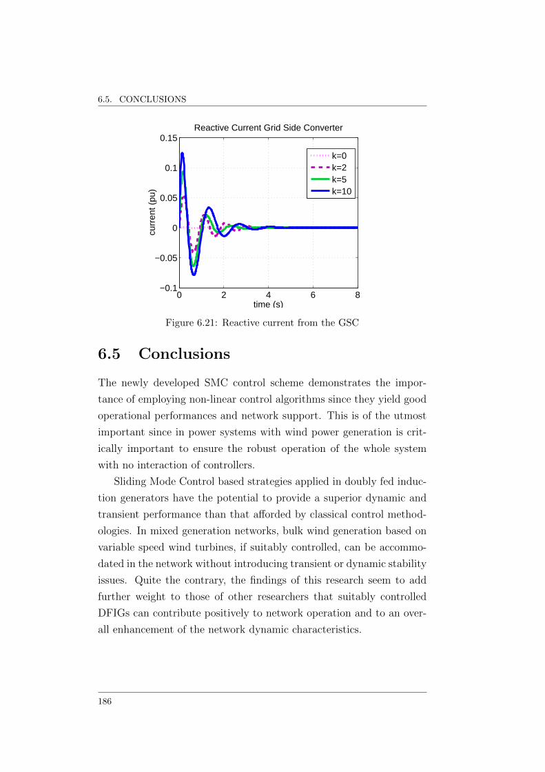
6.5. CONCLUSIONS
0 2 4 6 8−0.1
−0.05
0
0.05
0.1
0.15Reactive Current Grid Side Converter
time (s)
cur
rent
(pu
)
k=0k=2k=5k=10
Figure 6.21: Reactive current from the GSC
6.5 Conclusions
The newly developed SMC control scheme demonstrates the impor-
tance of employing non-linear control algorithms since they yield good
operational performances and network support. This is of the utmost
important since in power systems with wind power generation is crit-
ically important to ensure the robust operation of the whole system
with no interaction of controllers.
Sliding Mode Control based strategies applied in doubly fed induc-
tion generators have the potential to provide a superior dynamic and
transient performance than that afforded by classical control method-
ologies. In mixed generation networks, bulk wind generation based on
variable speed wind turbines, if suitably controlled, can be accommo-
dated in the network without introducing transient or dynamic stability
issues. Quite the contrary, the findings of this research seem to add
further weight to those of other researchers that suitably controlled
DFIGs can contribute positively to network operation and to an over-
all enhancement of the network dynamic characteristics.
186

Chapter 7
General Conclusions and
Future Research Avenues
This research work has addressed the timely issue of the dynamic per-
formance assessment of DFIG Wind Energy Conversion Systems, with
particular reference to its control system and the impact of the wind
power plant on the electrical power grid and vice-versa. The work has
been carried out in connection with a DFIG-WECS connected to an
equivalent strong system to investigate the issue of local oscillation
modes within the wind power plant itself and in a combined multi-
machine power system environment to investigate the issue of inter-
area modes.
A non-linear DFIG controller based on Sliding Mode Control was
proposed and its performance compared with that of a classical con-
troller based on Field Oriented Control. Sliding Mode Control showed
to be more robust and flexible than the classical controller, opening
the door for a more widespread future participation of DFIG-WECS in
the damping of power system oscillations. Modal analysis and time do-
main simulations were chosen to good effect as the study methods with
which to interpret the responses of the dynamic models addressed in
this research. They encompass both one DFIG-WECS connected to an
equivalent strong system and the case of a multi-machine power system
187
including conventional generation and DFIG-WECS. In both cases the
aim has been to assess the impact of wind turbine generator control
in system stability, particularly in electromechanical oscillations damp-
ing. The assessment has been rather comprehensive, including different
electrical grid topologies operating under a wide range of power gener-
ation scenarios.
The most significant findings and contributions of this thesis to-
gether with future avenues of research works in this area of electrical
power systems research are given below:
It has been found rather useful in order to contextualize the impor-
tance of the research, to have started by examining the general aspects
of power system stability and to have written down definitions and spe-
cific stability concepts in order to bring into the discussion, at a later
stage in the thesis, the contribution that DFIG-WECS and SMC will
make to power systems operation in the not too distant future. In the
same tenor, it was also deemed important to outline the most relevant
wind turbine components models available for power system dynamics,
with reference to small-signal and transient stability analyses.
The new application of Sliding Mode Control has been compre-
hensive not only in the sense that it encompasses both the machine
side converter and the grid side converter but also in the sense that it
has been applied to cases of multi-machine power systems containing a
combination of conventional synchronous generation and variable speed
wind power generators. Moreover, a wide range of operating scenarios
was considered and the new control strategy based on SMC, which is
non-linear, showed a very robust performance. A case in point is the
generator model and control strategies for the study of small-signal
stability of a wind turbine generator connected to an equivalent grid,
presented in Chapter 4. The modal analysis results for this simplified
representation of the power grid correctly include the effects of oper-
188

CHAPTER 7. GENERAL CONCLUSIONS AND FUTURE RESEARCHAVENUES
ating conditions, machine parameters and models, grid strength and
control system strategy. The results obtained corroborate that oper-
ating conditions, machine and system parameters affect markedly the
location and nature of the oscillatory modes but also that the control
approach adopted plays a major role. More specifically, it was found
that stability of the DFIG-based wind turbine using FOC depends to a
large extent on the tuning of the proportional-integral controllers and
on having good knowledge of the machine parameters - a change in
operating scenarios or system topology may require a re-tuning of the
proportional-integral controllers. Conversely, it was found that SMC is
a very convenient vehicle to improve on the DFIG stability; it showed
to be very robust under machine parameter and network variations.
It yields electro-mechanical coupling cancellation without introducing
additional modes and provides extra-damping which, in turn, reduces
local oscillations. In brief, SMC presents a far better performance than
the classical controller FOC, in this application.
Since the integration of wind power generators in the power grid
is on the increase, particularly the integration of wind power genera-
tion systems with double-fed induction generators, having a solid un-
derstanding of the impact that these generators will have on system
stability, is a current issue of paramount importance. Comprehensive
computer simulation studies have been carried out to gain a greater
insight into the benefits or otherwise of using variable-speed wind tur-
bine in mixed generation systems to improve on the stability of the
overall power networks. FOC- and SMC-based strategies were used to
evaluate the contribution that the controllers of the wind power gen-
eration units were able to exert on network damping. This showed the
effectiveness that SMC has in enhancing the dynamic performance of
the DFIG plant as well as the great potential that it has in drawing an
even superior dynamic performance of grid connected wind turbines.
This was further corroborated by carrying out transient studies using
time domain simulations of multi-machine power systems with embed-
ded wind power generation. It was found that the best control strategy
189

7.1. FUTURE RESEARCH AVENUES
was: (i) to apply SMC in the machine side converter to control the ro-
tor voltage in order to operate the wind turbine at optimum efficiency,
at the desired power factor; (ii) to apply SMC in the grid side converter
to maximize the damping of electromechanical oscillations by drawing
on its reactive power capability - the control law was derived using a
defined Lyapunov function. More punctually, the multi-machine power
system studies carried out in this research indicate the following:
• That a double fed induction generator has the potential to pro-
vide a superior dynamic and transient performance than that of
a conventional synchronous generator
• That in mixed generation networks, bulk wind generation based
on variable speed wind turbines, if suitably controlled, can be
accommodated on a network without introducing transient or
dynamic stability issues and that they can contribute positively
to network operation and contribute to an overall enhancement
of the network dynamic characteristics
• That the newly developed SMC control scheme demonstrates the
importance of employing non-linear control algorithms since they
yield good operational performances and network support. This
is the most important since in power systems with wind power
generation is critically important to ensure the robust operation
of the whole system with no interaction of controllers.
7.1 Future Research Avenues
Concerning recommendations for future research in this area of elec-
trical power systems, the following topics seem a natural extension of
this research:
• The proposed SMC control should be implemented in larger elec-
trical power systems, including networks with a higher degree of
complexity
190

CHAPTER 7. GENERAL CONCLUSIONS AND FUTURE RESEARCHAVENUES
• In order to test the performance of the sliding mode control
approach in a real-time, a suitable laboratory environment and
eventually a field-trial implementation ought to be carried out
• To take full advantage of the flexibility offered by the SMC, it
looks a rather attractive proposition to apply it other wind power
generation technologies such as the full power-converter system
191

7.1. FUTURE RESEARCH AVENUES
192

Bibliography
[1] M. J. Novogradac, Renewable Energy Tax Credit Handbook - 2010
Edition. Novogradac & Company LLP.
[2] V. Climate Policy Initiative, U. Varadarajan, and C. Initiative,
“A comparative Case-Study analysis of the effectiveness and effi-
ciency of policies that influence the financing of renewable energy
projects: US and europe,”
[3] “Global wind report 2010,” tech. rep., Global WindEnergy Coun-
cil - GWEC:, 2010.
[4] A. Mendonca and J. A. Lopes, “Impact of large scale wind power
integration on small signal stability,” in 2005 International Con-
ference on Future Power Systems, pp. 5 pp.–5, IEEE, Nov. 2005.
[5] O. Anaya-Lara, N. Jenkins, J. Ekanayake, P. Cartwright, and
M. Hughes, Wind Energy Generation: Modelling and Control.
Wiley, 1 ed., Sept. 2009.
[6] V. Utkin, J. Guldner, and J. Shi, Sliding Mode Control in Electro-
Mechanical Systems, Second Edition. CRC Press, 2 ed., May
2009.
[7] A. Sabanovic, L. Fridman, S. K. Spurgeon, and I. o. E. Engineers,
Variable structure systems: from principles to implementation.
IET, 2004.
193

BIBLIOGRAPHY
[8] W. Lee, M. Chen, J. Gim, K. Yoshimura, and S. Wang, “Dynamic
stability analysis of an industrial power system,” IEEE Transac-
tions on Industry Applications, vol. 31, pp. 675–681, Aug. 1995.
[9] “Proposed terms & definitions for power system stability,” IEEE
Transactions on Power Apparatus and Systems, vol. PAS-101,
pp. 1894–1898, July 1982.
[10] P. Kundur, J. Paserba, V. Ajjarapu, G. Andersson, A. Bose,
C. Canizares, N. Hatziargyriou, D. Hill, A. Stankovic, C. Taylor,
T. Van Cutsem, and V. Vittal, “Definition and classification of
power system stability IEEE/CIGRE joint task force on stability
terms and definitions,” IEEE Transactions on Power Systems,
vol. 19, pp. 1387– 1401, Aug. 2004.
[11] K. R. Padiyar, Power System Dynamics: Stability and Control.
John Wiley & Sons Ltd (Import), Pap/Dsk ed., Apr. 1999.
[12] “Power oscillation protection,” Nov. 2002.
[13] K. Prasertwong, N. Mithulananthan, and D. Thakur, “Under-
standing low-frequency oscillation in power systems,” Interna-
tional Journal of Electrical Engineering Education, vol. 47, no. 3,
pp. 248–262, 2010.
[14] Y. N. N. Tchokonte, Real-time Identification and Monitoring of
the Voltage Stability Margin in Electric Power Transmission Sys-
tems Using Synchronized Phasor Measurements. PhD thesis,
Kassel University, Germany, 2009.
[15] Taylor, Power System Voltage Stability. McGraw-Hill Education,
Sept. 1994.
[16] T. v. Cutsem and C. Vournas, Voltage Stability of Electric Power
Systems. Springer, 1 ed., Mar. 1998.
194

BIBLIOGRAPHY
[17] N. R. Ullah, T. Thiringer, and D. Karlsson, “Voltage and tran-
sient stability support by wind farms complying with the E.ON
netz grid code,” IEEE Transactions on Power Systems, vol. 22,
pp. 1647–1656, Nov. 2007.
[18] E. Vittal, M. O’Malley, and A. Keane, “A Steady-State volt-
age stability analysis of power systems with high penetrations of
wind,” IEEE Transactions on Power Systems, vol. 25, pp. 433–
442, Feb. 2010.
[19] J. Morren, S. W. de Haan, W. L. Kling, and J. A. Ferreira,
“Wind turbines emulating inertia and supporting primary fre-
quency control,” IEEE Transactions on Power Systems, vol. 21,
pp. 433– 434, Feb. 2006.
[20] G. Ramtharan, J. B. Ekanayake, and N. Jenkins, “Frequency
support from doubly fed induction generator wind turbines,” IET
Renewable Power Generation, vol. 1, pp. 3–9, Mar. 2007.
[21] P. Kundur, Power System Stability and Control. McGraw-Hill
Professional, Jan. 1994.
[22] L. L. Grigsby, The electric power engineering handbook. CRC
Press, 2001.
[23] J. Machowski, J. W. Bialek, and J. R. Bumby, Power system
dynamics and stability. John Wiley & Sons, Oct. 1997.
[24] P. W. Sauer and M. A. Pai, Power System Dynamics and Stabil-
ity. Prentice Hall, 1st ed., July 1997.
[25] L. Wang, F. Howell, P. Kundur, C. Y. Chung, and W. Xu, “A
tool for small-signal security assessment of power systems,” in
22nd IEEE Power Engineering Society International Conference
on Power Industry Computer Applications, 2001. PICA 2001. In-
novative Computing for Power - Electric Energy Meets the Mar-
ket, pp. 246–252, IEEE, 2001.
195
BIBLIOGRAPHY
[26] U. Kerin, T. N. Tuan, E. Lerch, and G. Bizjak, “Small signal se-
curity index for contingency classification in dynamic security as-
sessment,” in PowerTech, 2011 IEEE Trondheim, pp. 1–6, IEEE,
June 2011.
[27] S. Yang, F. Liu, D. Zhang, S. Mei, and G. He, “Polynomial ap-
proximation of the damping-ratio-based small-signal security re-
gion boundaries of power systems,” in 2011 IEEE Power and
Energy Society General Meeting, pp. 1–8, IEEE, July 2011.
[28] J. Paserba et al., “Analysis and control of power system oscilla-
tion,” CIGRE special publication, vol. 38, no. 07, 1996.
[29] G. C. Verghese, I. J. Perez-Arriaga, and F. C. Schweppe, “Se-
lective modal analysis with applications to electric power sys-
tems, part II: the dynamic stability problem,” IEEE Transactions
on Power Apparatus and Systems, vol. PAS-101, pp. 3126–3134,
Sept. 1982.
[30] I. J. Perez-Arriaga, G. C. Verghese, and F. C. Schweppe, “Selec-
tive modal analysis with applications to electric power systems,
PART i: Heuristic introduction,” IEEE Transactions on Power
Apparatus and Systems, vol. PAS-101, pp. 3117–3125, Sept. 1982.
[31] J. G. F. Francis, “The QR transformation a unitary analogue to
the LR Transformation-Part 1,” The Computer Journal, vol. 4,
pp. 265 –271, Jan. 1961.
[32] J. G. F. Francis, “The QR Transformation-Part 2,” The Com-
puter Journal, vol. 4, pp. 332 –345, Jan. 1962.
[33] J. H. Wilkinson, The algebraic eigenvalue problem. Clarendon
Press, 1988.
[34] R. T. Byerly, R. J. Bennon, and D. E. Sherman, “Eigenvalue
analysis of synchronizing power flow oscillations in large electric
196

BIBLIOGRAPHY
power systems,” IEEE Transactions on Power Apparatus and
Systems, vol. PAS-101, pp. 235–243, Jan. 1982.
[35] L. Wang and A. Semlyen, “Application of sparse eigenvalue
techniques to the small signal stability analysis of large power
systems,” in Power Industry Computer Application Conference,
1989. PICA ’89, Conference Papers, pp. 358–365, IEEE, May
1989.
[36] P. Kundur, G. J. Rogers, D. Y. Wong, L. Wang, and M. G.
Lauby, “A comprehensive computer program package for small
signal stability analysis of power systems,” IEEE Transactions
on Power Systems, vol. 5, pp. 1076–1083, Nov. 1990.
[37] J. I. Perez Arriaga, “Selective modal analysis with applications
to electric power systems,” s, Fred C. Schweppe and George C.
Verghese., Massachusetts Institute of Technology. Dept. of Elec-
trical Engineering and Computer Science., Massachusetts Insti-
tute of Technology. Dept. of Electrical Engineering and Computer
Science., 1981.
[38] M. Pai, Energy Function Analysis for Power System Stability.
Springer, 1 ed., Aug. 1989.
[39] F. A. Rahimi, M. G. Lauby, J. N. Wrubel, and K. L. Lee, “Evalu-
ation of the transient energy function method for on-line dynamic
security analysis,” IEEE Transactions on Power Systems, vol. 8,
pp. 497–507, May 1993.
[40] A. D. Patton, “Assessment of the security of operating electric
power systems using probability methods,” Proceedings of the
IEEE, vol. 62, pp. 892– 901, July 1974.
[41] Slootweg, Wind Power: Modelling and Impact on Power System
Dynamics. PhD thesis, Electrical Engineering, Mathematics and
Computer Science, Delft University of Technology, Dec. 2003.
197

BIBLIOGRAPHY
[42] J. Ekanayake and N. Jenkins, “Comparison of the response of
doubly fed and fixed-speed induction generator wind turbines to
changes in network frequency,” IEEE Transactions on Energy
Conversion, vol. 19, pp. 800– 802, Dec. 2004.
[43] P. W. Carlin, A. S. Laxson, and E. B. Muljadi, “The history and
state of the art of Variable-Speed wind turbine technology,” tech.
rep., NREL, National Renewable Energy Laboratory, February
2001.
[44] S. Muller, M. Deicke, and R. W. De Doncker, “Doubly fed induc-
tion generator systems for wind turbines,” IEEE Industry Appli-
cations Magazine, vol. 8, pp. 26–33, June 2002.
[45] E. B. Muhando, T. Senjyu, E. Omine, T. Funabashi, and C. Kim,
“Modelling-based approach for digital control design for nonlin-
ear WECS in the power system,” Wind Energy, vol. 13, pp. 543–
557, Sept. 2010.
[46] T. Ackermann, Wind power in power systems. John Wiley and
Sons, Mar. 2005.
[47] A. Hansen, P. Sorensen, F. Iov, and F. Blaabjerg, “Control of
variable speed wind turbines with doubly-fed induction genera-
tors,” Wind Engineering, vol. 28, pp. 411–432, June 2004.
[48] J. G. Slootweg, H. Polinder, and W. L. Kling, “Representing wind
turbine electrical generating systems in fundamental frequency
simulations,” IEEE Transactions on Energy Conversion, vol. 18,
pp. 516– 524, Dec. 2003.
[49] J. G. Slootweg, S. W. de Haan, H. Polinder, and W. L. Kling,
“General model for representing variable speed wind turbines
in power system dynamics simulations,” IEEE Transactions on
Power Systems, vol. 18, pp. 144– 151, Feb. 2003.
198
BIBLIOGRAPHY
[50] B.O.E, “Procedimiento de operacion PO 12.3. requisitos de re-
spuesta frente a huecos de tension de las instalaciones electricas
(in spanish),” tech. rep., 2006.
[51] F. K. Lima, A. Luna, P. Rodriguez, E. H. Watanabe, and
F. Blaabjerg, “Rotor voltage dynamics in the doubly fed induc-
tion generator during grid faults,” IEEE Transactions on Power
Electronics, vol. 25, pp. 118–130, Jan. 2010.
[52] J. Slootweg and W. Kling, “The impact of large scale wind power
generation on power system oscillations,” Electric Power Systems
Research, vol. 67, pp. 9–20, Oct. 2003.
[53] L. Holdsworth, X. G. Wu, J. B. Ekanayake, and N. Jenkins,
“Comparison of fixed speed and doubly-fed induction wind tur-
bines during power system disturbances,” Generation, Transmis-
sion and Distribution, IEE Proceedings-, vol. 150, pp. 343– 352,
May 2003.
[54] J. J. Sanchez-Gasca, N. W. Miller, and W. W. Price, “A modal
analysis of a two-area system with significant wind power pen-
etration,” in Power Systems Conference and Exposition, 2004.
IEEE PES, pp. 1148– 1152 vol.2, IEEE, Oct. 2004.
[55] F. M. Hughes, O. Anaya-Lara, N. Jenkins, and G. Strbac, “A
power system stabilizer for DFIG-based wind generation,” IEEE
Transactions on Power Systems, vol. 21, pp. 763– 772, May 2006.
[56] E. Muljadi, C. P. Butterfield, B. Parsons, and A. Ellis, “Effect
of variable speed wind turbine generator on stability of a weak
grid,” IEEE Transactions on Energy Conversion, vol. 22, pp. 29–
36, Mar. 2007.
[57] J. M. Rodriguez, J. L. Fernandez, D. Beato, R. Iturbe, J. Usaola,
P. Ledesma, and J. R. Wilhelmi, “Incidence on power system
dynamics of high penetration of fixed speed and doubly fed wind
199

BIBLIOGRAPHY
energy systems: study of the spanish case,” IEEE Transactions
on Power Systems, vol. 17, pp. 1089– 1095, Nov. 2002.
[58] F. W. Koch, I. Erlich, F. Shewarega, and U. Bachmann, “Dy-
namic interaction of large offshore wind farms with the elec-
tric power system,” in Power Tech Conference Proceedings, 2003
IEEE Bologna, vol. 3, IEEE, June 2003.
[59] P. Ledesma and J. Usaola, “Doubly fed induction generator
model for transient stability analysis,” IEEE Transactions on
Energy Conversion, vol. 20, pp. 388– 397, June 2005.
[60] Y. Chi, Y. Liu, W. Wang, and H. Dai, “Voltage stability analysis
of wind farm integration into transmission network,” in Interna-
tional Conference on Power System Technology, 2006. PowerCon
2006, pp. 1–7, IEEE, Oct. 2006.
[61] A. D. Hansen and G. Michalke, “Fault ride-through capability of
DFIG wind turbines,” Renewable Energy, vol. 32, pp. 1594–1610,
July 2007.
[62] V. Bufano, M. Dicorato, A. Minoia, and M. Trovato, “Embed-
ding wind farm generation in power system transient stability
analysis,” in Power Tech, 2005 IEEE Russia, pp. 1–7, IEEE,
June 2005.
[63] H. Gaztanaga, I. Etxeberria-Otadui, S. Bacha, and D. Roye,
“Fixed-Speed wind farm operation improvement by using DVR
devices,” in IEEE International Symposium on Industrial Elec-
tronics, 2007. ISIE 2007, pp. 2679–2684, IEEE, June 2007.
[64] C. Alvarez, H. Amaris, O. Samuelsson, D. Florez, and L. Gon-
zalez, “Custom power systems and software platforms for wind
farms under voltage dips situations,” in Universities Power En-
gineering Conference, 2008. UPEC 2008. 43rd International,
pp. 1–4, IEEE, Sept. 2008.
200
BIBLIOGRAPHY
[65] C. Angeles-Camacho, E. Farinas-Wong, and F. Banuelos-Ruedas,
“FACTS: its role in the connection of wind power to power net-
works,” in Modern Electric Power Systems (MEPS), 2010 Pro-
ceedings of the International Symposium, pp. 1–7, IEEE, Sept.
2010.
[66] L. Holdsworth, J. B. Ekanayake, and N. Jenkins, “Power system
frequency response from fixed speed and doubly fed induction
generator-based wind turbines,” Wind Energy, vol. 7, pp. 21–35,
Jan. 2004.
[67] G. Lalor, A. Mullane, and M. O’Malley, “Frequency control and
wind turbine technologies,” IEEE Transactions on Power Sys-
tems, vol. 20, pp. 1905– 1913, Nov. 2005.
[68] R. Doherty, A. Mullane, G. Nolan, D. J. Burke, A. Bryson, and
M. O’Malley, “An assessment of the impact of wind generation
on system frequency control,” IEEE Transactions on Power Sys-
tems, vol. 25, pp. 452–460, Feb. 2010.
[69] N. R. Ullah, T. Thiringer, and D. Karlsson, “Temporary pri-
mary frequency control support by variable speed wind turbines-
potential and applications,” IEEE Transactions on Power Sys-
tems, vol. 23, pp. 601–612, May 2008.
[70] N. R. Ullah, Wind Power - Added Value for Network Operation.
PhD thesis, Chalmers University Of Technology, Goteborg, Swe-
den, 2008.
[71] A. Mullane and M. O’Malley, “The inertial response of Induction-
Machine-Based wind turbines,” IEEE Transactions on Power
Systems, vol. 20, pp. 1496– 1503, Aug. 2005.
[72] R. G. de Almeida and J. A. Lopes, “Participation of doubly fed
induction wind generators in system frequency regulation,” IEEE
Transactions on Power Systems, vol. 22, pp. 944–950, Aug. 2007.
201
BIBLIOGRAPHY
[73] E. Vittal, J. D. McCalley, V. Ajjarapu, and T. Harbour, “Wind
penetration limited by thermal constraints and frequency stabil-
ity,” in Power Symposium, 2007. NAPS ’07. 39th North Ameri-
can, pp. 353–359, IEEE, Oct. 2007.
[74] R. Fernandez, R. Mantz, and P. Battaiotto, “Impact of wind
farms on a power system. an eigenvalue analysis approach,” Re-
newable Energy, vol. 32, pp. 1676–1688, Aug. 2007.
[75] J. M. Mauricio, A. Marano, A. Gomez-Exposito, and J. L.
Martinez Ramos, “Frequency regulation contribution through
Variable-Speed wind energy conversion systems,” IEEE Trans-
actions on Power Systems, vol. 24, pp. 173–180, Feb. 2009.
[76] O. Anaya-Lara, F. M. Hughes, N. Jenkins, and G. Strbac, “Con-
tribution of DFIG-based wind farms to power system short-term
frequency regulation,” Generation, Transmission and Distribu-
tion, IEE Proceedings-, vol. 153, pp. 164– 170, Mar. 2006.
[77] D. A. Spera, Wind turbine technology: fundamental concepts of
wind turbine engineering. ASME Press, May 2009.
[78] E. Hau, Wind Turbines: Fundamentals, Technologies, Applica-
tion, Economics. Springer, 2nd ed., Oct. 2005.
[79] J. Zhou, E. Erdem, G. Li, and J. Shi, “Comprehensive evaluation
of wind speed distribution models: A case study for north dakota
sites,” Energy Conversion and Management, vol. 51, pp. 1449–
1458, July 2010.
[80] M. Mohanpurkar and R. G. Ramakumar, “Probability density
functions for power output of wind electric conversion systems,”
in 2010 IEEE Power and Energy Society General Meeting, pp. 1–
7, IEEE, July 2010.
[81] A. Ouammi, V. Ghigliotti, M. Robba, A. Mimet, and R. Sacile,
“A decision support system for the optimal exploitation of wind
202

BIBLIOGRAPHY
energy on regional scale,” Renewable Energy, vol. 37, pp. 299–
309, Jan. 2012.
[82] R. Bansal, T. Bhatti, and D. Kothari, “On some of the design
aspects of wind energy conversion systems,” Energy Conversion
and Management, vol. 43, pp. 2175–2187, Nov. 2002.
[83] J. L. R. Amenedo, Analisis Dinamico y Diseno del Sistema de
Control de Aeroturbinas de Velocidad Variable con Generador
Asıncrono de Doble Alimentacion (in spanish). PhD thesis, Car-
los III de Madrid, Leganes, Madrid, 2000.
[84] C. Vilar Moreno, Fluctuaciones de tension producidas por los
aerogeneradores de velocidad fija (in spanish). PhD thesis, Carlos
III de Madrid, Leganes, Madrid, 2002.
[85] L. Helle, Modeling and Comparison of Power Converters for Dou-
bly Fed Induction Generators in Wind Turbines. Institut for En-
ergiteknik, Aalborg Universitet, 2007.
[86] T. Burton, Wind energy: handbook. John Wiley and Sons, Dec.
2001.
[87] M. O. L. Hansen, Aerodynamics of wind turbines. Earthscan,
Feb. 2008.
[88] S. K. Salman and A. L. Teo, “Windmill modeling consideration
and factors influencing the stability of a grid-connected wind
power-based embedded generator,” IEEE Transactions on Power
Systems, vol. 18, pp. 793– 802, May 2003.
[89] S. K. Salman, A. L. Teo, and I. M. Rida, “The effect of shaft
modelling on the assessment of fault CCT and the power quality
of a wind farm,” in Ninth International Conference on Harmonics
and Quality of Power, 2000. Proceedings, vol. 3, pp. 994–998
vol.3, IEEE, 2000.
203

BIBLIOGRAPHY
[90] E. N. Hinrichsen and P. J. Nolan, “Dynamics and stability of
wind turbine generators,” IEEE Transactions on Power Appara-
tus and Systems, vol. PAS-101, pp. 2640–2648, Aug. 1982.
[91] R. Pena, J. C. Clare, and G. M. Asher, “Doubly fed induction
generator using back-to-back PWM converters and its applica-
tion to variable-speed wind-energy generation,” Electric Power
Applications, IEE Proceedings -, vol. 143, pp. 231–241, May 1996.
[92] I. Takahashi and T. Noguchi, “A new Quick-Response and High-
Efficiency control strategy of an induction motor,” IEEE Trans-
actions on Industry Applications, vol. IA-22, pp. 820–827, Sept.
1986.
[93] L. Xu and P. Cartwright, “Direct active and reactive power con-
trol of DFIG for wind energy generation,” IEEE Transactions on
Energy Conversion, vol. 21, pp. 750–758, Sept. 2006.
[94] L. Holdsworth, X. G. Wu, J. B. Ekanayake, and N. Jenkins, “Di-
rect solution method for initialising doubly-fed induction wind
turbines in power system dynamic models,” Generation, Trans-
mission and Distribution, IEE Proceedings-, vol. 150, pp. 334–
342, May 2003.
[95] W. Leonhard, Control of Electrical Drives. Springer, 3nd ed.,
Sept. 2001.
[96] F. Valenciaga, P. F. Puleston, and S. K. Spurgeon, “A geometric
approach for the design of MIMO sliding controllers. application
to a wind driven double output induction generator,” in Interna-
tional Workshop on Variable Structure Systems, 2006. VSS’06,
pp. 115–120, IEEE, June 2006.
[97] T. Lund, P. Sorensen, and J. Eek, “Reactive power capability
of a wind turbine with doubly fed induction generator,” Wind
Energy, vol. 10, pp. 379–394, July 2007.
204
BIBLIOGRAPHY
[98] L. Fernandez, C. Garcia, and F. Jurado, “Comparative study on
the performance of control systems for doubly fed induction gen-
erator (DFIG) wind turbines operating with power regulation,”
Energy, vol. 33, pp. 1438–1452, Sept. 2008.
[99] Y. Tang and L. Xu, “A flexible active and reactive power control
strategy for a variable speed constant frequency generating sys-
tem,” IEEE Transactions on Power Electronics, vol. 10, pp. 472–
478, July 1995.
[100] M. V. Nunes, J. A. Lopes, H. H. Zurn, U. H. Bezerra, and
R. G. Almeida, “Influence of the variable-speed wind generators
in transient stability margin of the conventional generators inte-
grated in electrical grids,” IEEE Transactions on Energy Con-
version, vol. 19, pp. 692– 701, Dec. 2004.
[101] J. Hu, H. Nian, B. Hu, Y. He, and Z. Q. Zhu, “Direct active and
reactive power regulation of DFIG using Sliding-Mode control
approach,” IEEE Transactions on Energy Conversion, vol. 25,
pp. 1028–1039, Dec. 2010.
[102] X. Zheng, L. Li, D. Xu, and J. Platts, “Sliding mode MPPT
control of variable speed wind power system,” in Power and En-
ergy Engineering Conference, 2009. APPEEC 2009. Asia-Pacific,
pp. 1–4, IEEE, Mar. 2009.
[103] S. Z. Chen, N. C. Cheung, K. C. Wong, and J. Wu, “Integral
Sliding-Mode direct torque control of Doubly-Fed induction gen-
erators under unbalanced grid voltage,” IEEE Transactions on
Energy Conversion, vol. 25, pp. 356–368, June 2010.
[104] M. I. Martinez, G. Tapia, A. Susperregui, and H. Camblong,
“Sliding-Mode control for DFIG rotor- and Grid-Side convert-
ers under unbalanced and harmonically distorted grid voltage,”
IEEE Transactions on Energy Conversion, vol. PP, no. 99, pp. 1–
12.
205

BIBLIOGRAPHY
[105] “World wind energy association, wwea 2010,
http://www.wwindea.org.”
[106] N. Jenkins, R. Allan, P. Crossley, D. Kirschen, and G. Strbac,
Embedded Generation (IEE Power)PBPO0310. Institution of En-
gineering and Technology, July 2000.
[107] D. Gautam, L. Goel, R. Ayyanar, V. Vittal, and T. Harbour,
“Control strategy to mitigate the impact of reduced inertia due to
doubly fed induction generators on large power systems,” IEEE
Transactions on Power Systems, vol. 26, pp. 214–224, Feb. 2011.
[108] M. Klein, G. Rogers, and P. Kundur, “A fundamental study of
inter-area oscillations in power systems,” IEEE Transactions on
Power Systems, vol. 6, pp. 914–921, Aug. 1991.
[109] T. Petru and T. Thiringer, “Modeling of wind turbines for power
system studies,” IEEE Transactions on Power Systems, vol. 17,
pp. 1132– 1139, Nov. 2002.
[110] Y. Lei, A. Mullane, G. Lightbody, and R. Yacamini, “Modeling
of the wind turbine with a doubly fed induction generator for grid
integration studies,” IEEE Transactions on Energy Conversion,
vol. 21, pp. 257– 264, Mar. 2006.
[111] J. B. Ekanayake, L. Holdsworth, X. Wu, and N. Jenkins, “Dy-
namic modeling of doubly fed induction generator wind tur-
bines,” IEEE Transactions on Power Systems, vol. 18, pp. 803–
809, May 2003.
[112] M. Rahimi and M. Parniani, “Transient performance improve-
ment of wind turbines with doubly fed induction generators us-
ing nonlinear control strategy,” IEEE Transactions on Energy
Conversion, vol. 25, pp. 514–525, June 2010.
[113] B. Beltran, T. Ahmed-Ali, and M. E. Benbouzid, “Sliding mode
power control of variable speed wind energy conversion systems,”
206
BIBLIOGRAPHY
in Electric Machines & Drives Conference, 2007. IEMDC ’07.
IEEE International, vol. 2, pp. 943–948, IEEE, May 2007.
[114] F. Valenciaga, P. F. Puleston, and P. E. Battaiotto, “Variable
structure system control design method based on a differential
geometric approach: application to a wind energy conversion
subsystem,” Control Theory and Applications, IEE Proceedings
-, vol. 151, pp. 6– 12, Jan. 2004.
[115] F. Wu, X. P. Zhang, K. Godfrey, and P. Ju, “Small signal stabil-
ity analysis and optimal control of a wind turbine with doubly
fed induction generator,” IET Generation, Transmission & Dis-
tribution, vol. 1, pp. 751–760, Sept. 2007.
[116] M. Al-Biati, M. El-Kady, and A. Al-Ohaly, “Dynamic stabil-
ity improvement via coordination of static var compensator and
power system stabilizer control actions,” Electric Power Systems
Research, vol. 58, pp. 37–44, May 2001.
[117] Z. Elrazaz and A. A. Al-Ohaly, “Optimal coordination of shunt
reactors to enhance system performance at light load operation,”
Generation, Transmission and Distribution, IEE Proceedings C,
vol. 140, pp. 293–298, July 1993.
[118] E. Z. Zhou, “Application of static VAr compensators to increase
power system damping,” IEEE Transactions on Power Systems,
vol. 8, pp. 655–661, May 1993.
[119] C. Wang, L. Shi, L. Wang, and Y. Ni, “Small signal stability
analysis considering grid-connected wind farms of DFIG type,”
in 2008 IEEE Power and Energy Society General Meeting - Con-
version and Delivery of Electrical Energy in the 21st Century,
pp. 1–6, IEEE, July 2008.
[120] G. Tsourakis, B. Nomikos, and C. Vournas, “Effect of wind parks
with doubly fed asynchronous generators on small-signal stabil-
207

BIBLIOGRAPHY
ity,” Electric Power Systems Research, vol. 79, pp. 190–200, Jan.
2009.
[121] D. Gautam, V. Vittal, and T. Harbour, “Impact of increased
penetration of DFIG-Based wind turbine generators on transient
and small signal stability of power systems,” IEEE Transactions
on Power Systems, vol. 24, pp. 1426–1434, Aug. 2009. cc.
[122] Y. Mishra, S. Mishra, F. Li, Z. Y. Dong, and R. C. Bansal,
“Small-Signal stability analysis of a DFIG-Based wind power sys-
tem under different modes of operation,” IEEE Transactions on
Energy Conversion, vol. 24, pp. 972–982, Dec. 2009.
[123] S. Yuanzhang, W. Lixin, L. Guojie, and L. Jin, “A review on
analysis and control of small signal stability of power systems
with large scale integration of wind power,” in 2010 International
Conference on Power System Technology (POWERCON), pp. 1–
6, IEEE, Oct. 2010.
[124] J. L. Rueda and I. Erlich, “Impacts of large scale integration of
wind power on power system small-signal stability,” in 2011 4th
International Conference on Electric Utility Deregulation and Re-
structuring and Power Technologies (DRPT), pp. 673–681, IEEE,
July 2011.
[125] Z. Miao, L. Fan, D. Osborn, and S. Yuvarajan, “Control of DFIG-
Based wind generation to improve interarea oscillation damping,”
IEEE Transactions on Energy Conversion, vol. 24, pp. 415–422,
June 2009.
[126] L. Fan, H. Yin, and Z. Miao, “On Active/Reactive power mod-
ulation of DFIG-Based wind generation for interarea oscillation
damping,” IEEE Transactions on Energy Conversion, vol. 26,
pp. 513–521, June 2011.
[127] N. Kshatriya, U. D. Annakkage, F. M. Hughes, and A. M. Gole,
“Optimized partial eigenstructure Assignment-Based design of a
208
BIBLIOGRAPHY
combined PSS and active damping controller for a DFIG,” IEEE
Transactions on Power Systems, vol. 25, pp. 866–876, May 2010.
[128] K. Elkington, M. Ghandhari, and L. Soder, “Using power system
stabilisers in doubly fed induction generators,” in Power Engi-
neering Conference, 2008. AUPEC ’08. Australasian Universi-
ties, pp. 1–6, IEEE, Dec. 2008.
[129] L. Fan, Z. Miao, and D. Osborn, “Impact of doubly fed wind
turbine generation on inter-area oscillation damping,” in 2008
IEEE Power and Energy Society General Meeting - Conversion
and Delivery of Electrical Energy in the 21st Century, pp. 1–8,
IEEE, July 2008.
[130] C. Martinez, G. Joos, and B. T. Ooi, “Power system stabilizers
in variable speed wind farms,” in IEEE Power & Energy Society
General Meeting, 2009. PES ’09, pp. 1–7, IEEE, July 2009.
[131] N. R. Ullah and T. Thiringer, “Effect of operational modes of a
wind farm on the transient stability of nearby generators and on
power oscillations: a nordic grid study,” Wind Energy, vol. 11,
pp. 63–73, Jan. 2008.
[132] W. Qiao and R. G. Harley, “Effect of grid-connected DFIG wind
turbines on power system transient stability,” in 2008 IEEE
Power and Energy Society General Meeting - Conversion and
Delivery of Electrical Energy in the 21st Century, pp. 1–7, IEEE,
July 2008.
[133] J. Slootweg and W. Kling, “Modelling and analysing impacts
of wind power on transient stability of power systems,” Wind
Engineering, vol. 26, pp. 3–20, Jan. 2002.
[134] K. Elkington, V. Knazkins, and M. Ghandhari, “On the stabil-
ity of power systems containing doubly fed induction generator-
based generation,” Electric Power Systems Research, vol. 78,
pp. 1477–1484, Sept. 2008.
209

BIBLIOGRAPHY
[135] M. Rahimi and M. Parniani, “Dynamic behavior analysis of
doubly-fed induction generator wind turbines -the influence of
rotor and speed controller parameters,” International Journal of
Electrical Power & Energy Systems, vol. 32, pp. 464–477, June
2010.
[136] F. M. Hughes, O. Anaya-Lara, N. Jenkins, and G. Strbac, “Con-
trol of DFIG-based wind generation for power network support,”
IEEE Transactions on Power Systems, vol. 20, pp. 1958– 1966,
Nov. 2005.
[137] A. Luna, F. K. de Araujo Lima, D. Santos, P. Rodriguez, E. H.
Watanabe, and S. Arnaltes, “Simplified modeling of a DFIG for
transient studies in wind power applications,” IEEE Transactions
on Industrial Electronics, vol. 58, pp. 9–20, Jan. 2011.
[138] H. A. Pulgar-Painemal and P. W. Sauer, “Reduced-order model
of Type-C wind turbine generators,” Electric Power Systems Re-
search, vol. 81, pp. 840–845, Apr. 2011.
[139] S. Foster, L. Xu, and B. Fox, “Coordinated reactive power
control for facilitating fault ride through of doubly fed induc-
tion generator- and fixed speed induction generator-based wind
farms,” IET Renewable Power Generation, vol. 4, pp. 128–138,
Mar. 2010.
[140] I. Erlich, J. Kretschmann, J. Fortmann, S. Mueller-Engelhardt,
and H. Wrede, “Modeling of wind turbines based on Doubly-Fed
induction generators for power system stability studies,” IEEE
Transactions on Power Systems, vol. 22, pp. 909–919, Aug. 2007.
[141] S. Engelhardt, J. Kretschmann, J. Fortmann, F. Shewarega,
I. Erlich, and C. Feltes, “Negative sequence control of DFG based
wind turbines,” in 2011 IEEE Power and Energy Society General
Meeting, pp. 1–8, IEEE, July 2011.
210

BIBLIOGRAPHY
[142] G. Monsees, Discrete-Time Sliding Mode Control. PhD thesis,
Delft University of Technology, 2002.
[143] V. Utkin and A. Zinober, “Variable structure and lyapunov con-
trol,” vol. 193 of Lecture Notes in Control and Information Sci-
ences, pp. 87–107, Springer Berlin / Heidelberg, 1994.
[144] A. Isidori, Nonlinear Control Systems. Birkhauser, Aug. 1995.
[145] P. Kachroo and K. Ozbay, “Sliding mode for user equilibrium dy-
namic traffic routing control,” in Intelligent Transportation Sys-
tem, 1997. ITSC ’97., IEEE Conference on, pp. 70 –75, Nov.
1997.
[146] Q. Khan, A. I. Bhatti, S. Iqbal, and M. Iqbal, “Dynamic inte-
gral sliding mode for MIMO uncertain nonlinear systems,” In-
ternational Journal of Control, Automation and Systems, vol. 9,
pp. 151–160, Feb. 2011.
[147] M. Fliess, “Nonlinear control theory and differential algebra,” in
Modelling and Adaptive Control (C. Byrnes and A. Kurzhanski,
eds.), vol. 105 of Lecture Notes in Control and Information Sci-
ences, pp. 134–145, Springer Berlin / Heidelberg, 1988.
[148] X. Yan, C. Edwards, S. Spurgeon, and J. Bleijs, “Decentralised
sliding-mode control for multimachine power systems using only
output information,” Control Theory and Applications, IEE Pro-
ceedings -, vol. 151, pp. 627 – 635, Sept. 2004.
[149] L. Jiang, Q. Wu, and J. Wen, “Decentralized nonlinear adaptive
control for multimachine power systems via high-gain perturba-
tion observer,” Circuits and Systems I: Regular Papers, IEEE
Transactions on, vol. 51, pp. 2052 – 2059, Oct. 2004.
[150] F. Pourboghrat, F. Farid, C. Hatziadoniu, M. Daneshdoost,
F. Mehdian, and M. Lotfalian, “Local sliding control for damping
211

BIBLIOGRAPHY
interarea power oscillations,” Power Systems, IEEE Transactions
on, vol. 19, pp. 1123 – 1134, May 2004.
[151] P. M. Anderson and A. A. Fouad, Power System Control and
Stability. Wiley-IEEE Press, 2 ed., Oct. 2002.
212