
Docteur de l’Universit e Lille 1: sciences et...
130
N ◦ 41841 UNIVERSIT ´ E DE LILLE 1 SCIENCES ET TECHNOLOGIES ´ Ecole Doctorale Sciences Pour l’Ing´ enieur TH ` ESE pour obtenir le grade de Docteur de l’Universit´ e Lille 1: sciences et technologies Sp´ ecialit´ e: Micro et Nanotechnologies, Acoustique et T´ el´ ecommunications pr´ epar´ ee ` a l’Institut d’Electronique de Micro´ electronique et de Nanotechnologie pr´ esent´ ee et soutenue publiquement le 27 novembre 2015 par: Farah ZAAROUR Channel estimation algorithms for OFDM in interference scenarios Membres du jury Rapporteurs: Pr. Daniel ROVIRAS CNAM Paris Pr. Christophe LAOT Telecom Bretagne Examinateur: Dr. Mohammad-Ali KHALIGHI Ecole Centrale Marseille Pr. J´ erˆ ome LOUVEAUX Universit´ e catholique de Louvain Directeurs de th` ese: Pr. Martine LIENARD Universit´ e de Lille Pr. Iyad DAYOUB Universit´ e de Valenciennes Encadrants: Dr. Eric SIMON Universit´ e de Lille Dr. Marie COLIN-ZWINGELSTEIN Universit´ e de Valenciennes
Transcript of Docteur de l’Universit e Lille 1: sciences et...

N 41841
UNIVERSITE DE LILLE 1 SCIENCES ET TECHNOLOGIES
Ecole Doctorale Sciences Pour l’Ingenieur
THESE
pour obtenir le grade de
Docteur de l’Universite Lille 1: sciences et technologies
Specialite: Micro et Nanotechnologies, Acoustique et Telecommunicationspreparee a l’Institut d’Electronique de Microelectronique et de Nanotechnologie
presentee et soutenue publiquement le 27 novembre 2015 par:
Farah ZAAROUR
Channel estimation algorithms for OFDM in interferencescenarios
Membres du jury
Rapporteurs:
Pr. Daniel ROVIRAS CNAM ParisPr. Christophe LAOT Telecom BretagneExaminateur:Dr. Mohammad-Ali KHALIGHI Ecole Centrale MarseillePr. Jerome LOUVEAUX Universite catholique de LouvainDirecteurs de these:Pr. Martine LIENARD Universite de LillePr. Iyad DAYOUB Universite de ValenciennesEncadrants:Dr. Eric SIMON Universite de LilleDr. Marie COLIN-ZWINGELSTEIN Universite de Valenciennes

2

3
To my family ... ♥

Acknowledgments
This thesis, as any journey in life, has been full with moments of doubt,anxiety and uncertainty. It has also been full with moments of success, achieve-ment and confidence. During both times, I was lucky to have the support of alot of people whom I would like to acknowledge. This is to let them know thatthis work could not have been achieved without them.
First, it is thanks to God, Allah, for the courage, patience and guidance Hegave me to begin, persist and finalize this journey.
I am particularly grateful to professor Daniel ROVIRAS and professorChristophe LAOT for accepting to be the reviewers of my manuscript and forthe quality of their reviews on my work. I am also grateful to professor JeromeLOUVEAUX and doctor Mohammad-Ali KHALIGHI for their commitment tobe part of my jury committee.
I would like to thank everyone in TELICE, for their warm welcome, friend-liness and sense of humor. Thanks to professor Martine LIENARD for hostingme in the lab.
My sincere appreciation goes to doctor Eric SIMON. I would like to thankhim not only for his availability and for the particular effort and support heprovided me during my thesis, but also for his patience, kindness and for hisconfidence in me during the most difficult times. Thanks to our discussions, Ihave learned much more than science during my stay.
I would like to thank Emmanuelle GILLMANN for her unconditional helpfrom my first days in France.
4

5
I would also like to thank professor Iyad DAYOUB and doctor MarieCOLIN-ZWINGELSTEIN from the university of Valenciennes for the time theydevoted to me and for their constructive comments on my work, but most ofall for their conviviality.
My gratitude goes to my colleagues and friends in Lebanon and France fortheir support and for all the times we have spent together. Thanks to Hawraa,Hiba, Dina, Nora, Faten, Walaa, Hassanein, Mortada, Raouf, Shiqi, HuaqiangShu, Kyoko, Khaled and to all those they know I consider them as friends.
Finally, I would like to thank my family in Lebanon and USA for their sup-port and their participation, each one in his special way to make this possible.
To my father, mother and sisters: Dunia, Leila and Dana, this is for you...
Resume
La rarete du spectre radio et la demande croissante de bande passanterendent l’optimisation de l’utilisation du spectre essentiel. Tandis qu’une ef-ficacite maximale devrait etre atteinte, un niveau minimal d’interference de-vrait etre maintenu. L’OFDM (Orthogonal Frequency Division Multiplexing enanglais) est un schema de modulation bien connu pour combattre efficacementl’evanouissement multi trajets. OFDM a ete retenu comme un schema de mod-ulation dans plusieurs normes, comme le 3GPP LTE (Long Term Evolutionen anglais) et un derive d’OFDM, le GFDM (Generalized Frequency DivisionMultiplexing en anglais), est un candidat pour le systeme 5G. L’estimationde canal est une tache fondamentale dans les systemes OFDM et elle devientplus difficile en presence d’interference. Dans cette these, notre objectif estde proposer des algorithmes d’estimation de canal pour les systemes OFDMen presence d’interference, ou les algorithmes classiques d’estimation de canalechouent. En particulier, nous nous concentrons sur les interferences dues acertaines approches utilisees pour optimiser le spectre. Cela nous amene a con-siderer les deux cas suivants.
1) Tout d’abord, nous considerons l’environnement radio intelligente CR(Cognitive Radio en anglais) qui a ete propose pour faire face au probleme derarete du spectre. Les technologies qui emploient l’OFDM comme schema demodulation (WIMAX, WRAN) peuvent exister dans un scenario de CR. Dansde tels scenarios, un type particulier d’interference se pose et il est connu commel’interference a bande etroite ou NBI (Narrowband Interference en anglais).NBI est caracterisee par une puissance elevee qui frappe un petit nombre desous porteuse dans un systeme OFDM. Pendant que tous les travaux dansla litterature traitent le cas du canal a variations lentes, nous proposons unnouveau cadre d’estimation de canal pour les canaux a variations rapides con-
6

7
tamines par NBI. Cela est accompli avec l’algorithme EM (Expectation maxi-mization en anglais) et une expression explicite pour l’estimation de la puis-sance du bruit est obtenue.
2) Une autre source de consommation de bande passante en OFDM estla presence de pilotes connus inseres dans la trame OFDM pour accomplirl’estimation du canal. Pour tenter de remedier a ce probleme, les pilotes super-poses SP (Superimposed Pilots en anglais) ont ete proposes comme substitutsaux pilotes classiques. Dans cette these, on est interesse par une nouvelle classede SP pour OFDM connu comme DNSP (Data Nulling SP en anglais). DNSPassure des pilotes sans interference au detriment d’interference des donnes. Duea la modernite de DNSP, un recepteur adapte a son design doit etre concu.Les recepteurs turbo sont connus pour etre les plus efficaces en supprimantl’interference. Neanmoins, ils possedent deux inconvenients majeurs; leur com-plexite et leur besoin d’un canal precis. La contribution de ce travail est doubleet elle est orientee vers le traitement des deux inconvenients mentionnes.
Nous proposons d’abord un annuleur d’interferences IC (Interference can-celer en anglais) base sur le critere MMSE (Minimum Mean Square Erroren anglais) a faible complexite pour DNSP. En fait, nous montrons qu’en ex-ploitant la structure specifique de l’interference en DNSP, l’inversion de matricenecessaire dans le cas classique se reduit a l’inversion d’une matrice diagonale.Cependant, la performance de l’IC propose n’est fiable que quand l’erreur del’estimation du canal est faible. Donc, dans une autre contribution, nous pro-posons un IC pour DNSP en tenant compte des erreurs d’estimation du canal.
Enfin l’estimation robuste du canal est abordee dans le dernier chapitre.
Abstract
The scarcity of the radio spectrum and the increasing demand on band-width makes it vital to optimize the spectrum use. While a maximum effi-ciency should be attained, a minimal interference level should be maintained.Orthogonal frequency division multiplexing (OFDM) is a well-known modula-tion scheme reputed to combat multipath fading efficiently. OFDM has beenselected as the modulation scheme in several standards such as the 3GPP longterm evolution (LTE) and a derivative of OFDM, the generalized frequencydivision multiplexing (GFDM), is a candidate for 5G systems. In order toguarantee a coherent detection at the receiver, in the absence of the channelknowledge, channel estimation is regarded as a fundamental task in OFDM. Itbecomes even more challenging in the presence of interference.
In this thesis, our aim is to propose channel estimation algorithms forOFDM systems in the presence of interference, where conventional channel es-timators designed for OFDM fail. In particular, we focus on interference thatarises as a result of schemes envisioned to optimize the spectrum use. Thisleads us to consider two main themes; cognitive radio (CR) and superimposedpilots (SP).
First, we consider the CR environment which has been proposed to tacklethe problem of spectrum scarcity. Technologies employing OFDM as their mod-ulation scheme such as WIMAX and WRAN, might exist in a CR network. Insuch scenarios, a particular type of interference arises and is known as thenarrowband interference (NBI). NBI is characterized by a high power whichstrikes a small number of OFDM sub-carriers. While all existing literatureaddresses slow time-varying channels, we propose a novel channel estimationframework for fast time-varying channels in OFDM with NBI. This is accom-plished through an expectation maximization (EM) based algorithm. Thisformulation allows us to obtain a closed-form expression for the noise power
8

9
estimation.The known pilot sub-carriers inserted within the OFDM frame to accom-
plish the channel estimation task are another source of bandwidth consumptionin OFDM. In an attempt to overcome this drawback, SP have been proposed assubstitutes to conventional pilots. In this thesis, we are particularly interestedin a very recent class of SP for OFDM, known as the data-nulling SP (DNSP)scheme. DNSP assures interference-free pilots at the expense of data interfer-ence. Seen the modernity of DNSP, a suitable receiver has to be designed tocope with its design. Turbo receivers are well known to be the most efficientin canceling interference. However, two main drawbacks of turbo receivers aretheir high complexity and their need of an accurate channel estimate. The con-tribution of this work is twofold and is oriented to deal with the two mentioneddownsides of turbo receivers.
We first propose a low-complexity soft approximated minimum mean squareerror (MMSE) interference canceler (IC) particularly for DNSP. In fact, weshow that by exploiting the specific interference structure that arises in DNSP,the matrix inversion needed by the approximated MMSE-IC in the classical casereduces to a diagonal matrix inversion. The performance of the proposed IC isreliable when the channel estimation error is small. As another contribution, weextend the design of the approximated IC for DNSP so as to take the channelestimation errors into account. Those two contributions allow us to benefitfrom the interference cancellation property of turbo receivers, while keeping alow-complexity and dealing with channel estimation errors when present.
Finally, robust channel estimation is discussed in the last chapter. In par-ticular, we provide some insights and propositions for its implementation toproblems of channel estimation in OFDM.

Contents
Liste des figures 12
List of variables, notations and acronyms 16List of variables . . . . . . . . . . . . . . . . . . . . . . . . . . . . . . 16List of notations . . . . . . . . . . . . . . . . . . . . . . . . . . . . . 21List of acronyms (in alphabetical order) . . . . . . . . . . . . . . . . 22
Introduction 26
1 Introduction to OFDM 311.1 Introduction . . . . . . . . . . . . . . . . . . . . . . . . . . . . . 311.2 Propagation Model . . . . . . . . . . . . . . . . . . . . . . . . . 32
1.2.1 Typical propagation model . . . . . . . . . . . . . . . . 321.2.2 Multipath Fading . . . . . . . . . . . . . . . . . . . . . . 331.2.3 Channel Model . . . . . . . . . . . . . . . . . . . . . . 35
1.2.3.1 Deterministic Modeling . . . . . . . . . . . . . 361.2.3.2 Random Modeling . . . . . . . . . . . . . . . . 36
1.3 OFDM System Model . . . . . . . . . . . . . . . . . . . . . . . 371.3.1 Introduction . . . . . . . . . . . . . . . . . . . . . . . . 371.3.2 Transmission Chain and mathematical representation . 37
1.4 Channel Estimation in OFDM . . . . . . . . . . . . . . . . . . 411.5 Conclusion . . . . . . . . . . . . . . . . . . . . . . . . . . . . . 42
2 EM-based Channel Estimation for OFDM Contaminated byNarrow Band Interference 432.1 Introduction and Motivation . . . . . . . . . . . . . . . . . . . . 442.2 Coexistence in the Frequency Spectrum . . . . . . . . . . . . . 46
10

CONTENTS 11
2.2.1 The IEEE 802.11g WLAN and Bluetooth . . . . . . . . 47
2.2.2 The IEEE 802.11g WRAN in TV White Space . . . . . 47
2.3 Expectation Maximization Algorithm . . . . . . . . . . . . . . 48
2.3.1 Introduction . . . . . . . . . . . . . . . . . . . . . . . . 48
2.3.2 Mathematical Formulation of EM . . . . . . . . . . . . 49
2.3.3 Extension to the EM-MAP Algorithm . . . . . . . . . . 49
2.4 OFDM System Model with NBI . . . . . . . . . . . . . . . . . 51
2.4.1 BEM Channel Model . . . . . . . . . . . . . . . . . . . . 52
2.4.2 The AR Model for ck . . . . . . . . . . . . . . . . . . . 53
2.5 Proposed Channel Estimator . . . . . . . . . . . . . . . . . . . 53
2.5.1 EM algorithm . . . . . . . . . . . . . . . . . . . . . . . . 54
2.5.2 Kalman Smoother . . . . . . . . . . . . . . . . . . . . . 55
2.6 Simulation results . . . . . . . . . . . . . . . . . . . . . . . . . 56
2.6.1 Algorithm Initialization . . . . . . . . . . . . . . . . . . 58
2.6.2 Comparison of Proposed Algorithm with Literature . . 58
2.6.3 Robustness of Proposed Algorithm to Model Mismatch 61
2.7 Complexity Comparison with Literature . . . . . . . . . . . . . 62
2.8 Conclusion . . . . . . . . . . . . . . . . . . . . . . . . . . . . . 63
3 A Low Complexity Turbo Receiver for Data-Nulling Superim-posed Pilots in OFDM 65
3.1 Introduction . . . . . . . . . . . . . . . . . . . . . . . . . . . . . 66
3.2 System Design . . . . . . . . . . . . . . . . . . . . . . . . . . . 67
3.2.1 Transmitter . . . . . . . . . . . . . . . . . . . . . . . . . 67
3.2.2 OFDM System Model . . . . . . . . . . . . . . . . . . . 69
3.3 DNSP transmission model . . . . . . . . . . . . . . . . . . . . . 70
3.4 Least Squares channel estimation . . . . . . . . . . . . . . . . . 71
3.4.1 Obtaining hk . . . . . . . . . . . . . . . . . . . . . . . . 71
3.4.2 Using hk . . . . . . . . . . . . . . . . . . . . . . . . . . 71
3.5 Proposed Iterative Receiver for DNSP . . . . . . . . . . . . . . 72
3.5.1 MMSE soft IC of the Literature . . . . . . . . . . . . . 72
3.5.2 Proposed Structure . . . . . . . . . . . . . . . . . . . . . 74
3.6 Simulation Results and Discussions . . . . . . . . . . . . . . . . 75
3.6.1 mismatched exact IC vs mismatched proposed IC . . . . 75
3.6.2 DNSP with mismatched proposed IC vs CSP in turboreception framework . . . . . . . . . . . . . . . . . . . . 78
3.6.2.1 Complexity Comparison . . . . . . . . . . . . . 81
3.6.2.2 Convergence . . . . . . . . . . . . . . . . . . . 83
3.7 Conclusion . . . . . . . . . . . . . . . . . . . . . . . . . . . . . 83

12 CONTENTS
4 A Low Complexity Turbo Receiver for DNSP in OFDM withchannel estimation errors 854.1 Introduction and Motivation . . . . . . . . . . . . . . . . . . . . 854.2 Improved exact IC for DNSP . . . . . . . . . . . . . . . . . . . 864.3 Improved proposed IC for DNSP . . . . . . . . . . . . . . . . . 884.4 Improved Approximated IC of [SKD09] . . . . . . . . . . . . . 904.5 Simulation results and discussions . . . . . . . . . . . . . . . . 914.6 Conclusion . . . . . . . . . . . . . . . . . . . . . . . . . . . . . 93
5 Perspectives: On Robust Estimation with bounded data un-certainties 945.1 Introduction and Motivation . . . . . . . . . . . . . . . . . . . . 945.2 The regularized LS and its robust counterpart . . . . . . . . . . 955.3 The Kalman filter and its robust counterpart . . . . . . . . . . 975.4 Ambiguities associated with the robust approach . . . . . . . . 1025.5 Conclusion . . . . . . . . . . . . . . . . . . . . . . . . . . . . . 103
Conclusion 105
Annexe 109
A Calculations related to chapter two 110A.1 Computation of the Q Function . . . . . . . . . . . . . . . . . . 110
A.2 Calculation of σ2n
(i+1). . . . . . . . . . . . . . . . . . . . . . . 111
A.3 Additional complexity calculation for proposed algorithm withrespect to algorithm in [HR10] . . . . . . . . . . . . . . . . . . 112
B Calculations related to chapter three 114B.1 Demonstration of equation (3.17) from (3.11) . . . . . . . . . . 114B.2 Complexity Computation of the mismatched exact IC and the
mismatched proposed IC . . . . . . . . . . . . . . . . . . . . . . 115B.2.1 Complexity of mismatched exact IC . . . . . . . . . . . 115B.2.2 Complexity of mismatched proposed IC . . . . . . . . . 116
C Calculations related to chapter four 118
D Calculations related to chapter 5 120
Bibliographie 123

List of Figures
1.1 Typical Propagation Scenario . . . . . . . . . . . . . . . . . . . 33
1.2 Fading channel classification . . . . . . . . . . . . . . . . . . . . 34
1.3 OFDM transmission chain . . . . . . . . . . . . . . . . . . . . . 38
1.4 Cyclic Prefix insertion in OFDM . . . . . . . . . . . . . . . . . 39
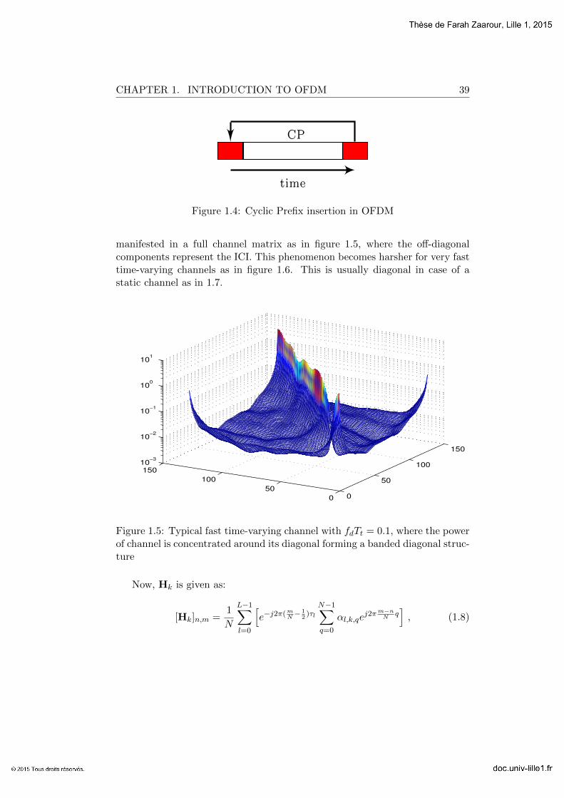
1.5 Typical fast time-varying channel with fdTt = 0.1, where thepower of channel is concentrated around its diagonal forming abanded diagonal structure . . . . . . . . . . . . . . . . . . . . . 39
1.6 Very fast time varying channel for fdTt = 0.5, where the powerof the channel is dispersed all over the sub-carrier indexes . . . 40
1.7 Static channel, i.e. fdTt = 0, where the power of channel isconcentrated on its diagonal entries . . . . . . . . . . . . . . . . 41
2.1 WRAN deployment scenario . . . . . . . . . . . . . . . . . . . . 47
2.2 EM Algorithm [KML04] . . . . . . . . . . . . . . . . . . . . . . 50
2.3 Proposed Estimator . . . . . . . . . . . . . . . . . . . . . . . . 53
2.4 MSE performance for K = 2, SIR = 0 dB, fdTt = 0.05, Nc = 3 57
2.5 MSE performance for K = 2, SIR = 0 dB, fdTt = 0.05, Nc = 3 58
2.6 MSE performance for K = 2, SNR = 20 dB, SIR = 0 dB . . . . 59
2.7 MSE performance for K = 2, SNR = 20 dB, SIR = 0 dB . . . . 60
2.8 MSE performance for K = 2, SIR = 0 dB, SNR = 20 dB, Nc = 3 60
2.9 MSE performance for K = 2, SIR = 0 dB, fdTt = 0.05, Nc = 3 61
2.10 BER performance for K = 4, SIR = 0 dB, fdTt = 0.05, Nc = 3Lf = 8, #:iteration number . . . . . . . . . . . . . . . . . . . . 62
3.1 Transmitter-Receiver for SP schemes . . . . . . . . . . . . . . . 68
3.2 Schematic representation of the DNSP and CSP schemes . . . . 69
13

14 LIST OF FIGURES
3.3 Equalizer Block . . . . . . . . . . . . . . . . . . . . . . . . . . . 75
3.4 BER Performance for 4QAM & coding rate=12 . Solid line: mis-
matched proposed IC, line with asterisks: mismatched exact IC,#:number of iteration . . . . . . . . . . . . . . . . . . . . . . . 76
3.5 BER Performance for 16QAM & coding rate=12 . Solid line: mis-
matched proposed IC, line with asterisks: mismatched exact IC,#:number of iteration . . . . . . . . . . . . . . . . . . . . . . . 77
3.6 MSE Performance for CSP and DNSP , ρ = 0.125, Lf = 8#:number of iteration . . . . . . . . . . . . . . . . . . . . . . . 79
3.7 BER Performance for CSP and DNSP , ρ = 0.125, Lf = 8#:number of iteration . . . . . . . . . . . . . . . . . . . . . . . 80
3.8 BER Performance for CSP, DNSP and C-CSP, ρ = 0.125, Lf = 8#:number of iteration . . . . . . . . . . . . . . . . . . . . . . . 81
3.9 BER Performance for CSP, DNSP and C-CSP, ρ = 0.125, Lf =8, SNR = 12 . . . . . . . . . . . . . . . . . . . . . . . . . . . . 82
4.1 Matrix FFH with different values of L, N=128. . . . . . . . . . 87
4.2 BER performance of the sixth iteration for 4QAM, K = 2, L =15 dB, Lf = 8 for mismatched exact IC, mismatched proposedIC, improved exact IC, improved proposed IC and CSI . . . . . 89
4.3 BER performance of the sixth iteration for 16QAM, K = 3,L = 15 dB, Lf = 8 for mismatched exact IC, improved exact ICand CSI . . . . . . . . . . . . . . . . . . . . . . . . . . . . . . . 90
4.4 BER performance of the sixth iteration for 16QAM, K = 3, L =15 dB, Lf = 8 for mismatched proposed IC, improved proposedIC and CSI . . . . . . . . . . . . . . . . . . . . . . . . . . . . . 91
4.5 BER performance of the sixth iteration for 16QAM, K = 3, L =15 dB, Lf = 8 for improved proposed IC, improved approximatedof [SKD09] and CSI . . . . . . . . . . . . . . . . . . . . . . . . 92
4.6 BER performance of the sixth iteration for the improved proposedIC using Σk denoted full and by using only the diagonal elementsof Σk denoted diag (a) 4QAM (b) 16QAM . . . . . . . . . . . . 93
5.1 Error variance of three filters with ∆i selected uniformly withinthe interval [-1,1], T(1)=0.0198, F(1,2)=0.0196 . . . . . . . . . 98
5.2 Error variance of three filters with ∆i selected uniformly withinthe interval [-1,1], T(1)=0.198, F(1,2)=0.0196 . . . . . . . . . . 99
5.3 Error variance of three filters with ∆i selected uniformly withinthe interval [-1,1], T(1)=0.0198, F(1,2)=0.3912 . . . . . . . . . 100
5.4 G(λ) . . . . . . . . . . . . . . . . . . . . . . . . . . . . . . . . . 102

List of Tables
3.1 Complexity for different IC . . . . . . . . . . . . . . . . . . . . 773.2 Complexity Comparison for different SP schemes . . . . . . . . 82
A.1 Additional Complexity of the proposed algorithm . . . . . . . . 112
15

List of variables, notations andacronyms
List of variables
N Number of sub-carriers in an OFDM system
Ng Cyclic prefix length
NT = N +Ng Total number of samples in an OFDM block
Ts Sampling time in an OFDM frame
T = NTTs Total duration of an OFDM symbol
K Total number of OFDM symbols per frame
xk kth transmitted OFDM symbol
yk kth received OFDM symbol
Hk Channel matrix associated with the kth OFDM symbol
nk Additive white Gaussian noise on the kth OFDM sym-bol
σ2 Noise variance on sub-carrier n
16

LIST OF VARIABLES, NOTATIONS AND ACRONYMS 17
σ2TN Variance of thermal noise
σ2I,n Variance of unknown interference
Nc Number of BEM coefficients
σ2αl
Variance of the lth channel tap
αl,k,q lth channel tap sampled at time kTt + (q +Ng)Ts
L number of channel paths
B Basis function matrix
cl,k BEM coefficients
ξl,k BEM modeling error of the lth path on the kth OFDMsymbol
R(p)cl Correlation matrix of BEM coefficients
A and Ul AR parameters
c(i)k|k−1 BEM coefficients’ prediction
P(i)k|k−1 Prediction error covariance
Kk Kalman Gain
c(i)k|k BEM coefficients’ update
P(i)k|k Measurement error covariance

18 LIST OF VARIABLES, NOTATIONS AND ACRONYMS
A State Matrix
uk State Noise
fdTt Normalized Doppler frequency
Nc Number of BEM coefficients
hk Channel impulse response on kth OFDM symbol
hk Estimate of the channel impulse response on kth OFDMsymbol
D Number of data sub-carriers
P Number of pilot sub-carriers
Lf Distance between two adjacent pilots in frequency
W Hadamard matrix
ρ Pilot power allocation
yd,k kth received OFDM symbol on data sub-carriers
yp,k kth received OFDM symbol on pilot sub-carriers
np,k Noise on pilot sub-carriers of the kth OFDM symbol
nd,k Noise on data sub-carriers of the kth OFDM symbol
wk,n Channel equalizer for the kth OFDM symbol on thenth sub-carrier
sk,n Equalized symbol for the kth OFDM symbol on the nthsub-carrier
s′k,n Expected value of the data symbols given the LLR

LIST OF VARIABLES, NOTATIONS AND ACRONYMS 19
en N × 1 vector with one on its nth entry and zeros else-where
Vk,n N × N diagonal matrix with the variance of the softestimates on its entries
Wd D ×N sub-matrix of W
σ2s Variance of data symbols
σ2s Variance of estimated data symbols given the LLR
F N × L Fourier matrix
Fp P × L Fourier matrix
d Distance between transmitter and receiver
v Pathloss exponent
τm Delay spread
Bc Coherence bandwidth
fd Doppler frequency
Tc Coherence time
B Signal Bandwidth
τs Signal Symbol period
r(t) Continuous received signal in base band
s(t) Continuous transmitted signal in base band
τl Propagation delay associated with the lth path
20 LIST OF VARIABLES, NOTATIONS AND ACRONYMS
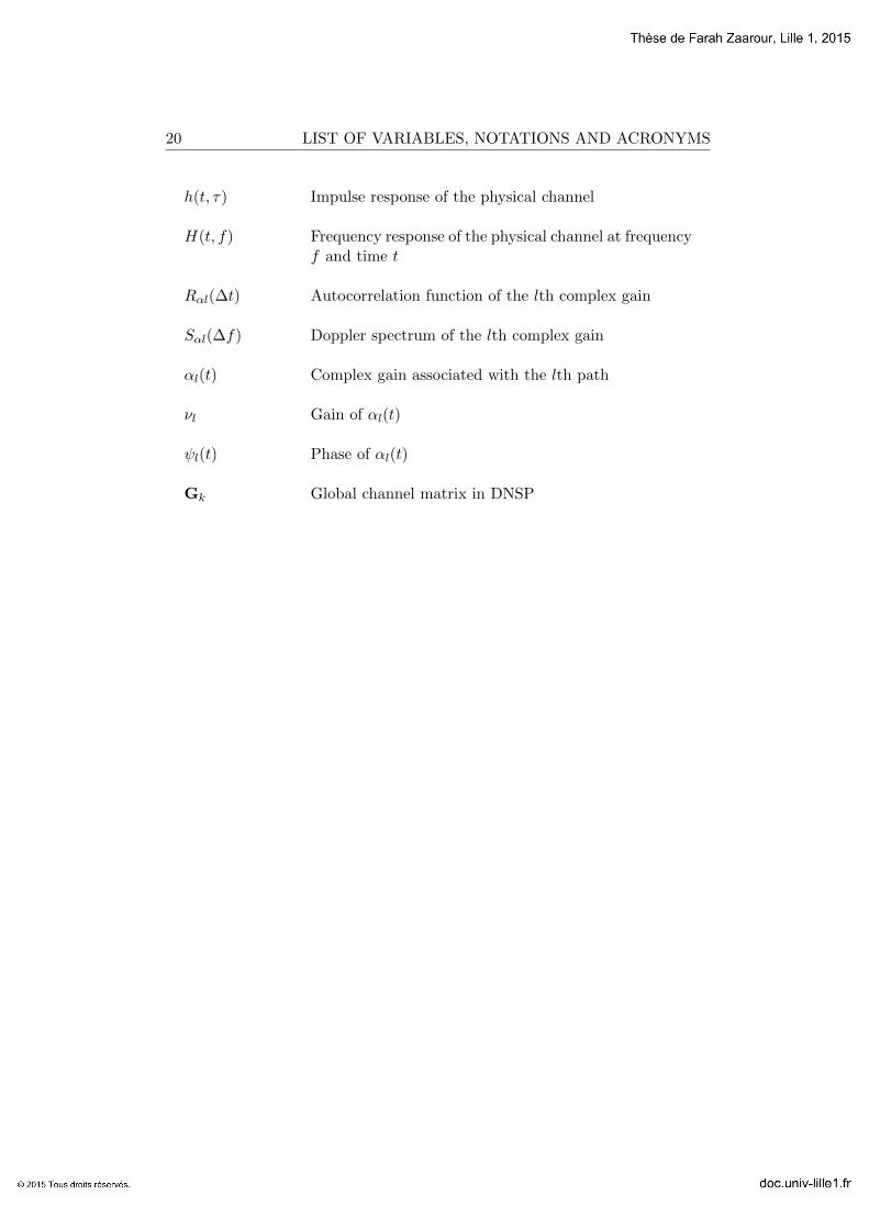
h(t, τ) Impulse response of the physical channel
H(t, f) Frequency response of the physical channel at frequencyf and time t
Rαl(∆t) Autocorrelation function of the lth complex gain
Sαl(∆f) Doppler spectrum of the lth complex gain
αl(t) Complex gain associated with the lth path
νl Gain of αl(t)
ψl(t) Phase of αl(t)
Gk Global channel matrix in DNSP

LIST OF VARIABLES, NOTATIONS AND ACRONYMS 21
List of notations
X Matrix X (bold capital letter )
x Vector x (bold small letter)
[X]n,m Element corresponding to the nth row and mth columnof matrix X
(·)T Transpose operator
(·)∗ Conjugate operator
(·)H Hermitian (conjugate transpose) operator
Tr(·) Trace
Ex,y[·] Expectation over x and y
δk,m Dirac function
arg max(.)
Maximum argument
diag(X) Vector with diagonal entries of matrix X
diag(x) Diagonal matrix with the entries of vector x on its di-agonal
FT Fourier transform operator
Hadamard multiplication

22 LIST OF VARIABLES, NOTATIONS AND ACRONYMS
List of acronyms (in alphabetical order)
ADSL Asynchronous digital subscriber line
AR Auto-regressive
AWGN Additive white Gaussian noise
BCRB Bayesian Cramer–Rao Bound
BDU bounded data uncertainty
BEM Basis Expansion Model
BER Bit Error Rate
BICM Bit-Interleaved Coded Modulation
CA Complex Addition
C-CSP coded classical superimposed pilots
CE Channel Estimation
CFO Carrier frequency offset
CIR Channel impulse response
CM Complex Multiplication
CMMOE Constrained Minimum Mean Output Energy
CP Cyclic Prefix
CR Cognitive Radio
CS Compressive sensing
CSI Channel State Information

LIST OF VARIABLES, NOTATIONS AND ACRONYMS 23
CSP Classical Superimposed Pilots
D/A (A/D) Digital to analog (Analog to digital )
DA Data-Aided
DFT Discrete Fourier Transform
DNSP Data Nulling Superimposed Pilots
ECM Expectation-Conditional Maximization
EM Expectation Maximization
FCC Federal Communications Commission
FFT Fast Fourier Transform
FT Fast Transform
GFDM Generalized Frequency Division Multiplexing
IC Interference Canceler
ICI Inter-carrier interference
IDFT Inverse DFT
IFFT Inverse Fast Fourier Transform
ISI Inter-symbol interference
ISM industrial, scientific and medical
LLR Log likelihood ratio
LMMSE Linear Minimum Mean Square Error

24 LIST OF VARIABLES, NOTATIONS AND ACRONYMS
LOS Line-of-sight
LS Least Squares
LTE Long Term Evolution
MAP Maximum a posteriori
ML Maximum Likelihood
MLE Maximum Likelihood Estimator
MMSE Minimum Mean Square Error
MSE Mean Square Error
MUE Measurement Update Equations
NBI Narrowband Interference
NLOS No Line-of-sight
NRNSC Non-Recursive Non-Systematic Convolutional
OFDM Orthogonal Frequency Division Multiplexing
P/S (S/P) Parallel to serial (Serial to parallel)
P-BEM Polynomial BEM
pdf probability density function
PEF Prediction Error Filter
PSAM Pilot-Symbol Assisted Modulation
PSIC Parallel Soft Interference Canceler
RA Real Addition

LIST OF VARIABLES, NOTATIONS AND ACRONYMS 25
RLS Regularized LS
RM Real Addition
SIR Signal-to-interference-ratio
SNR Signal-to-noise-ratio
SOS Second Order Statistics
SP Superimposed Pilots
TUE Time Update Equations
UFMC Universal Filtered Multi-Carrier
US Uncorrelated scatters
WLAN Wireless Local Area Network
WRAN Wireless Regional Area Network
WSS Wide-Sense Stationary

Introduction
The management of the spectrum is attributed to regulation authoritieswhich have the responsibility of organizing the frequency bands usage, so thatusers are guaranteed an acceptable quality of service. In particular, licensedusers are not supposed to encounter interference. However, measurements re-vealed that less than 40 % of the attributed spectrum is being fully used.This leaves an important portion of the spectrum reserved but underutilized.It reveals at the same time the inefficiency of the current regulation policieswhich offer licensed users the full access to the spectrum at all times. Whilebandwidth is a naturally scarce resource, and demands on higher data rates isin continuous increase, it becomes vital to make use of the wasted spectrum.Thus, optimizing the spectral efficiency becomes a priority in order to confrontthe scarcity of the spectrum on the one hand, and the demand of the constantlyemerging services on the other hand. We will hereafter discuss two approacheswhich will form the road-map to this thesis.
Cognitive radio (CR), first proposed in [Mit93], is based on the idea of spec-trum sharing. Its main idea is to allow secondary users to access the licensedspectrum when vacant. This sharing should be well organized (regulated) sothat the interference from secondary users on primary users is kept at its min-imal levels. This is usually assured by employing spectrum sensing capabilitiesin the CR networks so as to detect the availability of the spectrum beforetransmitting, thus avoiding interference.
While CR offers a solution to the spectrum underutilization caused by cur-rent regulation policies, there exists another source of bandwidth underutiliza-tion which is manifested by the use of known symbols (pilots) for the channelestimation task. This means that a non-negligible portion of the bandwidthis wasted rather than being assigned to useful symbols. Nevertheless, in orderto coherently acquire the channel at the receiver, some known symbols should
26

Introduction 27
be transmitted. To this end, superimposed pilots (SP) have been proposed toreplace classical pilots. In SP schemes, no bandwidth is exclusively dedicatedto pilots, but it is rather shared with unknown symbols (data) thus limitingthe loss in spectral efficiency.
Orthogonal frequency division multiplexing (OFDM) could be considered alandmark with strong foundations in the physical layer. It has been proposedto overcome the undesirable effect of inter-carrier interference and inter-symbolinterference and is perfectly adopted to mulipath channels; a typical scenarioin wireless transmission. Furthermore, OFDM is now standardized in severaltechnologies, ranging from wired to wireless communication and extending totelevision broadcasting transmissions. Consequently, and with reference to theabove discussion, systems employing OFDM as their access scheme might pos-sibly share the spectrum with other technologies. The channel estimation taskis no exception in OFDM systems, and is typically carried out via pilot-aidedalgorithms as discussed above.
We now narrow the rest of our discussion to OFDM, which is the modulationof interest in our thesis. In particular, our main concern in this thesis is toprovide solutions to channel estimation problems in OFDM in scenarios withinterference, where conventional channel estimation algorithms fail. We focuson interference that arises either from spectrum sharing (CR) between users,or from bandwidth sharing (SP) by the same user.
As it could be anticipated, optimizing the spectral efficiency, being it withthe employment of CR or with SP does not come without a cost. In fact, dif-ferent sources of interference should be dealt with at the receiver.
We first consider the CR environment with a fast time-varying OFDM chan-nel and conventional pilots. In CR, the spectrum sensing capabilities we al-ready mentioned can not guarantee an interference-free transmission. In fact,a particular kind of interference arises in OFDM when coexisting with othertechnologies. It is characterized by a high power over a small number of sub-carriers. This is known as the narrowband interference (NBI) and its presencerenders conventional channel estimators inefficient. This will be the focus ofour work in chapter 2.
Then, we consider a quasi-static OFDM channel with SP and an NBI-freeenvironment. The sharing of the bandwidth in SP schemes could be performedusing different approaches. In the classical SP (CSP) scheme, pilots are arith-metically added to data with a different power contribution. This leads tointerference on channel estimation from data and on data decoding from pi-
28 INTRODUCTION
lots. A more recent SP scheme, known as the data-nulling SP (DNSP) scheme,cancels the effect of data on pilots by first precoding the data and then nullingit as some positions for the insertion of pilots. This assures that there is no in-terference on pilots, yet, interference originates from data on themselves. Thiswill be the focus of our work in chapters 3 and 4.
Thesis Organization:
In chapter 1, we provide a brief overview of the multipath propagationchannel, the OFDM model in a fast time-varying scenario and a slow time-varying scenario and then briefly discuss conventional channel estimation tech-niques in OFDM.
In chapter 2, the fast time-varing OFDM channel model will be imple-mented and then adapted to include the NBI model. Extensive work on chan-nel estimation with NBI in OFDM systems exists in literature, but only in thecontext of low mobility. Thus, we present a novel framework to address theproblem of channel estimation in OFDM with NBI in high mobility conditions.In fact, the extension of this problem from low mobility scenarios to high mo-bility scenarios is not a direct one. Another motivation is the recent proposaldealing with the employment of CR in high speed railway in the CORRIDORproject [Cor]. This project is the first to address this topic in Europe in collab-oration with the Societe Nationale des Chemins de fer Francais (SNCF), whichis the French National Railway Company. To tackle this problem, we derive anEM-based channel estimator, in which the Kalman smoother is embedded. Wethen perform a comparison between the proposed algorithm and two algorithmsin the literature. In particular, the comparison is done with an algorithm thattakes into account NBI but neglects mobility and another which takes into ac-count mobility but neglects NBI. This comparison demonstrates the need of achannel estimator capable of dealing with NBI and mobility at the same time.We also calculate the additional complexity of the proposed algorithm whichis shown to be rather small compared to that of existing algorithms.
In chapter 3, the quasi-static OFDM channel model is used and adaptedthis time to include the DNSP model. DNSP is a recent proposal which emergedin 2014. It was thus essential to design a suitable receiver with an accept-able complexity. To this end, we propose a low-complexity turbo receiver forDNSP in OFDM. We then perform a comprehensive comparison with the CSPin OFDM within the turbo framework. This includes channel estimation, data

Introduction 29
decoding, and complexity comparisons. In fact, this study is of important prac-tical interest since it enables the designer to choose the pilot scheme dependingon the application and according to the desired trade-off between complexityand performance.
In chapter 4, we propose an improved low-complexity receiver for DNSPwhich takes the channel estimation errors into account. In the proposed re-ceiver of chapter 3, the channel estimate is used as if it were the true channel.This assumption has a low impact when small channel estimation errors arepresent, but it results in performance degradation otherwise.
Chapter 5 is devoted to the discussion of the possibility of implementingrobust estimators for the problem of channel estimation in OFDM. The robust-ness here refers to taking into account uncertainties in the model for a classof robust estimators known as the bounded data uncertainty (BDU) class. Infact, interference in the OFDM system such as the NBI in chapter 2 or the SPin chapter 3, could be viewed as uncertainties. In those two contexts, the con-ventional channel estimators fail due to the presence of those uncertainties andwe consequently had to design more elaborate techniques to deal with themat the receiver. Taking into account those certainties into the design of theestimator presents a new approach to deal with those problems. The contentof this chapter is to be viewed as a preliminary study which needs further de-velopments and is provided as a perspective for future research.
Publications:
The results of chapter 2 have been published in IEEE Wireless Commu-nications letters. Chapter 3 resulted in two conference publications, DICTAP2015 and BMSB 2015, and a paper under review in IET communications. Theapproach in chapter 4 has been submitted to IEEE Transactions on WirelessCommunications for review. Those are listed below:
F. Zaarour and E. Simon, ”Fast Time-Varying Channel Estimation forOFDM Systems with Narrowband Interference” IEEE Wireless Communica-tions Letters, vol.4 no. 4, pp. 389-392, 2015.
F. Zaarour, E. Simon, M. Zwingelstein-Colin, and I. Dayoub, ”A low com-plexity turbo receiver for data nulling superimposed pilots in OFDM,” FifthInternational Conference on Digital Information and Communication Technol-

30 INTRODUCTION
ogy and its Applications (DICTAP), pp.32,37, April 29 2015-May 1 2015.
F. Zaarour, E. Simon, M. Zwingelstein-Colin, and I. Dayoub, ”Compari-son of Superimposed Pilot Schemes in Iterative Receivers for OFDM Systems”IEEE International Symposium on Broadband Multimedia Systems and Broad-casting (BMSB), June 2015.
F. Zaarour, E. Simon, M. Zwingelstein-Colin, and I. Dayoub, ”On a Re-duced Complexity Iterative Receiver for Data Nulling Superimposed Pilots inOFDM”, under review in IET communications.
F. Zaarour, E. Simon, M. Zwingelstein-Colin, and I. Dayoub, ”An im-proved low Complexity Iterative Receiver for Data Nulling Superimposed Pi-lots in OFDM”, submitted to IEEE Transactions on Wireless Communications.

Chapter1Introduction to OFDM
Contents
1.1 Introduction . . . . . . . . . . . . . . . . . . . . . . . 31
1.2 Propagation Model . . . . . . . . . . . . . . . . . . . 32
1.2.1 Typical propagation model . . . . . . . . . . . . . . 32
1.2.2 Multipath Fading . . . . . . . . . . . . . . . . . . . . 33
1.2.3 Channel Model . . . . . . . . . . . . . . . . . . . . 35
1.2.3.1 Deterministic Modeling . . . . . . . . . . . 36
1.2.3.2 Random Modeling . . . . . . . . . . . . . . 36
1.3 OFDM System Model . . . . . . . . . . . . . . . . . . 37
1.3.1 Introduction . . . . . . . . . . . . . . . . . . . . . . 37
1.3.2 Transmission Chain and mathematical representation 37
1.4 Channel Estimation in OFDM . . . . . . . . . . . . . 41
1.5 Conclusion . . . . . . . . . . . . . . . . . . . . . . . . 42
1.1 Introduction
Orthogonal frequency division multiplexing (OFDM) is reputed for its abil-ity to mitigate multipath fading and enhance the spectral efficiency due toits orthogonal sub-carriers. This paved the way towards its presence in severalstandards today, ranging from wireless technologies such as the long term evolu-tion (LTE) in its downlink, to wired technologies such as the asynchronous dig-ital subscriber line (ADSL). However, the route towards standardization took
31

32 1.2. PROPAGATION MODEL
around 40 years. This dates back to the year 1966 when Cheng [Cha66] firstpresented the idea of transmitting parallel messages via a linear band-limitedchannel while maintaining an inter-carrier interference (ICI) free and inter-symbol interference (ISI) free transmission. Nevertheless, the major break-through which permitted the practical implementation of OFDM did not occurbefore the early 70’s when Weinstein and Ebert [WE71] introduced the use ofthe discrete Fourier transform (DFT) as an alternative to oscillators. However,their proposition did not address the orthogonality problem which was solved10 years later when Peled and Ruiz introduced the idea of the cyclic prefix(CP) [PR80]. Our goal in this chapter is to introduce the notions that willhelp clearly understand the channel models addressed in later chapters. Wefirst introduce the classical channel propagation model. Then, we present theOFDM system model and distinguish between the fast time-varying and thequasi-static channels. The former will provide a base for the system modelfor our discussion in chapter 2 while the latter will form the backbone for thesystem model in chapter 3. This will be followed by a discussion and a briefstate of the art of channel estimation techniques in OFDM. This discussion willhelp us establish the links and understand the motivations for the works pre-sented in later chapters since our ultimate goal is to estimate the channel at thereceiver with highest precision and efficiency (spectral) and lowest complexity.
1.2 Propagation Model
1.2.1 Typical propagation model
The basic structure of any communication system is composed of a transmit-ter, a propagation medium (channel) and a receiver. The propagation mediumcould be wired or wireless. We will be dealing with the latter in this thesis.In case of a fixed line of sight (LOS) transmission where the receiver has onlya single attenuated version of the transmitted signal, then directional anten-nas can be employed. However, a typical propagation scenario in a wirelessmedium leads to the reception of multiple copies of the transmitted signal atthe receiver with or without a LOS. A propagation scenario with a LOS com-ponent follows a Rice distribution while a propagation without a LOS followsa Rayleigh distribution.The propagation of an electromagnetic wave in a radio channel undergoes di-verse physical phenomenon. The three major mechanisms that impact thispropagation are the reflection, diffraction and scattering. Reflection occurswhen a propagating wave impinges upon a smooth surface with very largedimensions relative to its wavelength. Diffraction is produced when the propa-

CHAPTER 1. INTRODUCTION TO OFDM 33
gation path between the transmitter and the receiver is obstructed by a densebody with dimensions that are large relative to the signal’s wavelength, causingsecondary waves to be formed behind the obstructing body. It is often referredto as shadowing because the diffracted field can reach the receiver even whenshadowed by an impenetrable obstacle. Finally, scattering is produced whenthe radio wave falls on a surface whose dimensions are less than of the signal’swavelength, causing the energy to scatter in all directions. Those mechanism
Figure 1.1: Typical Propagation Scenario
lead to the reception of multiple copies of the transmitted signal at the receiver.Thus, the received is made up of the superposition of attenuated and delayedversions of the transmitted signal. A typical propagation scenario is illustratedin Figure 1.1. Those multiple paths characterize what is known as a multipathpropagation, and cause fluctuations in the received signal’s amplitude, phaseand angle of arrival, producing multipath fading. Thus the combination of theprimary signal with the delayed copies, leads to a constructive or destructive(fading) interference.
1.2.2 Multipath Fading
There exists two types of fading [B.S00]: large-scale fading and small-scalefading. Large-scale fading represents the average signal power attenuation or

34 1.2. PROPAGATION MODEL
pathloss due to motion over large areas. Hills, forests, and buildings situatedbetween the transmitter and the receiver might initiate this phenomenon. Prac-tically, this fading is characterized by statistics which provides a way of com-puting an estimate of the path-loss as a function of the distance. Precisely, thepathloss is proportional to 1
dv , where d is the distance between the transmitterand the receiver, and v is the pathloss exponent varying from 2 (free-space) to6 (urban environment). It is normally described in terms of mean path-loss anda log-normally distributed variation about the mean. Small-scale fading refers
Small Scale Fading
Time variation of channelTime spreading of signal
Time domain
Doppler-Shift
Frequencydomain
Time-Delay
Fast: Tc < τs
Slow: Tc > τs
Fast: fd > B
Slow: fd < B
F.Sel.: Bc < B
Flat: Bc > B
F.Sel.: τm > τs
Flat: τm < τs
FTFT
Figure 1.2: Fading channel classification
to the dramatic change in signal amplitude and phase that can be experiencedas a result of small changes in the spatial positioning between a receiver and atransmitter. In order to better understand this phenomenon, we introduce theparameters which characterize it. In particular, those are related to the timespreading of the signal and the time variation of the channel. The delay spreadτm is the difference between the arrival of the first and the last signal. The co-herence bandwidth Bc ≈ 1
τmis the range of frequencies over which the channel
is considered flat. Now, the Doppler spread is the spectral broadening causedby the relative motion of the receiver and transmitter, it is equal to the max-imum Doppler frequency (fd). The coherence time (Tc ≈ 1
fd) is the time over
which the channel is considered constant. The variations of those parametersdetermine the channel classification. In the frequency domain, when Bc > Bwhere B is the signal bandwidth, the channel undergoes flat or frequency nonselective fading. Its equivalent in the time-delay domain is observed when thedelay spread is much smaller than the signal symbol period τs i.e. τs > τm. Afrequency selective channel is produced when the inverse scenario occurs, eitherB > Bc in the frequency domain representation or τm > τs in the time-delayrepresentation. Fading can also be slow or fast 1. A fast fading scenario oc-curs when the coherence time of the channel is less than the symbol duration
1Fast fading is also referred to as time-selective fading.

CHAPTER 1. INTRODUCTION TO OFDM 35
Tc < τs as seen in the time domain or equivalently when the Doppler spreadis greater than the signal bandwidth fd > B in the frequency domain. Slowfading is produced when Tc > τs or fd < B. Those mechanisms are summarizedin Figure 1.2.
1.2.3 Channel Model
The received signal r(t) is composed of the different attenuated and delayedversions of the transmitted signal s(t). It is given in base band as:
r(t) =
L−1∑
l=0
αl(t)s(t− τl(t)) (1.1)
where L is the number of channel paths, τl(t) is the delay of each path withl = 0, ..., L− 1 and αl(t) is the amplitude or complex gain associated with thelth path. Thus, the impulse response of the channel as a function of time t anddelay τ is given as:
h(t, τ) =L−1∑
l=0
αl(t)δ(τ − τl(t)) (1.2)
where δ(τ) is the Dirac delta function. This formulation allows us to distinguishthree kinds of channel relative to the symbol duration τs:
• Static: The channel does not vary with time and is referred to as time-invariant
• Quasi-static: The channel is constant within a symbol but varies fromone symbol to another
• Time-varying: The channel varies within a symbol as well as from onesymbol to another.
Note that in this thesis, we consider that the number of channel paths L andthe delays τl(t), l = 0, ..., L− 1, are constant and known throughout the trans-mission of a frame of just a few symbols. In fact, the knowledge of thoseparameters is justified by the possibility to perform an initial estimation atthe beginning of the transmission [SRHG12]. In addition, the number of pathscould be considered constant due to the fact that the appearance and disap-pearance of paths are rare since those phenomena depend on the shadowingeffect which evolves slowly with respect to the symbol duration. Taking the

36 1.2. PROPAGATION MODEL
previous discussion into account, equation (1.2) could be re-written as:
h(t, τ) =L−1∑
l=0
αl(t)δ(τ − τl · Ts). (1.3)
Here, τl are the delays normalized by the sampling time Ts. It is obvious thatin order to resolve the transmitted signal at the receiver, the knowledge ofh(t, τ) is essential. This can be achieved assuming a deterministic or a randomchannel model.
1.2.3.1 Deterministic Modeling
There exists several ways to this approach. Measurement campaigns aimat measuring the channel impulse response at different points within the mea-surement perimeter. This, however, does not necessarily provide the channelcharacteristics such as the delays and paths. Nevertheless, it might be usefulfor network planning. With the development of the ray tracing technique whichis based on the idea of geometric optics, it became feasible to determine thetrajectory of the signals. This method can provide the propagation conditionsof a user for a given environment. However, it is sensitive to variations in thechannel.
1.2.3.2 Random Modeling
The random model of the channel depends directly on the classificationpresented in figure 1.2. The channel frequency response H(t, f) is directlylinked to the impulse response through the Fourier transform (FT) as:
H(t, f) =
∫ +∞
−∞h(t, τ)e−2jπfτdτ
=
L−1∑
l=0
αl(t)e−2jπfτlTs (1.4)
Classically, the impulse response is assumed to be wide-sense stationary (WSS)which indicates that each path αl(t) is a zero-mean complex Gaussian process;i.e. Eαl(t) = 0, with uncorrelated scatters (US) to indicate that the paths areuncorrelated i.e. Eαl1(t)αl
∗2(t) = 0. The WSSUS model was first introduced
by Bello in [Bel63]. Define ∆t = t1 − t2 as the time difference between tworealizations of the channel, then the complex amplitudes αl(t) could be modeledwith an autocorrelation function Rαl(∆t). Several models could be used to

CHAPTER 1. INTRODUCTION TO OFDM 37
model the channel, however, we focus here on the Rayleigh distribution sinceit is the one we will be using throughout this thesis. Thus, in a non-line-of-sight (NLOS) transmission, the signal is supposed to arrive from all differentdirections at the reception antenna. The channel is seen as the sum of nindependent random realizations. This could be expressed as:
αl(t) = νl(t)ejψl(t) =
∑
n
νl,nejψl,n(t). (1.5)
Applying the central limit theorem, αl(t) is Gaussian complex with gain |αl(t)|=νl that follows a Rayleigh distribution given as:
p(νl) =ν2l
σ2αl
e− ν2
l2σ2αl , (1.6)
and a uniformly distributed phase ψl(t) between 0 and 2π. Its variance, σ2αl
=E|αl(t)|2. Finally, the Doppler spectrum is obtained from Rαl(∆t) by theFourier Transform, i.e. Sαl(f) = FT(Rαl(∆t)) [Cla68].
1.3 OFDM System Model
1.3.1 Introduction
The basic idea behind OFDM is to transform a frequency selective channelinto N parallel sub-channels2 that undergo flat fading. In fact, one can directlyanticipate that the favorable scenario for transmission is to have slow flat fadingchannel conditions. This is guaranteed when fd < B < Bc. However, this isonly possible when fd · τm 1. Then, the symbol duration is chosen such thatτm < τs < Tc. Thus, in order to achieve high data rates, one would send alarge number of narrowband signals over relatively close frequencies. This is theexact rational behind multi-carrier transmission, which consequently facilitateschannel equalization at the receiver.
1.3.2 Transmission Chain and mathematical representation
In a classical OFDM system implemented with the DFT, we give the trans-mission chain in figure 1.3. We will consider frames composed of K OFDMsymbols. An OFDM symbol is the ensemble of the N narrowband signals. Weconsider the N × 1 vector of transmitted symbols on the kth OFDM symbol
2The terms sub-channel and sub-carrier are used interchangeably.

38 1.3. OFDM SYSTEM MODEL
Modulator S/P IFFT P/S add CP D/A
Channel
A/D
+
remove CPS/PFFTP/SDecoder
0, 1, ..., 1
0, 1, ..., 1
nk
Figure 1.3: OFDM transmission chain
xk =[xk,0, ..., xk,N−1
]Twith xk,n being the power-normalized transmitted
symbol on the sub-carrier n− N2 . Note that xk is obtained after the processing
of the binary data which are modulated an then passed through a serial toparallel (S/P) converter. xk is then fed to an N-point inverse DFT (IDFT)that transforms the data to the time domain which is again converted fromparallel to serial (P/S) . This allows us to insert the CP with length Ng whichis typically chosen to be larger than τm to avoid ISI. The CP is a repetition ofthe last part of the symbol at the beginning as depicted in figure 1.4.
Now, the total number of sub-carriers Nt = N +Ng and the total durationof each OFDM symbol is Tt = NtTs where Ts is the sampling time. The signalis then passed through a digital to analog (D/A) converter which containslow-pass filters with bandwidth 1
Ts. Then it is transmitted through the fading
channel where an additive white Gaussian noise (AWGN) nk of length N × 1with a covariance matrix defined as EnknHk = σ2
nI is added. At the receiver,the inverse of the operations performed at the transmitter are done. After the(A/D) converter, the cyclic prefix is removed, the stream is converted (S/P)and an N-DFT operation is performed to obtain the frequency domain receivedsignal yk which is given as:
yk = Hk xk + nk. (1.7)
The binary data is then recovered after channel decoding. The model in(1.7) is valid for any channel variation. However, the N ×N channel matrix ismodeled differently. We distinguish between time-varying channels, static andquasi-static channels. The time-varying channel destroys the orthogonalitybetween the sub-carriers and leads to inter-carrier interference (ICI). This is
CHAPTER 1. INTRODUCTION TO OFDM 39
time
CP
Figure 1.4: Cyclic Prefix insertion in OFDM
manifested in a full channel matrix as in figure 1.5, where the off-diagonalcomponents represent the ICI. This phenomenon becomes harsher for very fasttime-varying channels as in figure 1.6. This is usually diagonal in case of astatic channel as in 1.7.
0
50
100
150
0
50
100
150
10−3
10−2
10−1
100
101
Figure 1.5: Typical fast time-varying channel with fdTt = 0.1, where the powerof channel is concentrated around its diagonal forming a banded diagonal struc-ture
Now, Hk is given as:
[Hk]n,m =1
N
L−1∑
l=0
[e−j2π(m
N− 1
2)τl
N−1∑
q=0
αl,k,qej2πm−n
Nq], (1.8)

40 1.3. OFDM SYSTEM MODEL
0
50
100
150
0
50
100
150
10−4
10−3
10−2
10−1
100
101
Figure 1.6: Very fast time varying channel for fdTt = 0.5, where the power ofthe channel is dispersed all over the sub-carrier indexes
where αl,k,q = α(kTt + (q + Ng)Ts) is the lth channel tap sampled at timekTt + (q +Ng)Ts. In the case of static and quasi-static channels, Hk simplifiesto:
[Hk]n,n =
L−1∑
l=0
[αl,ke
−j2π( nN− 1
2)τl], (1.9)
where αl,k = α(kTt + (Ng + N2 )Ts). This formulation is based on the fact that
in static and quasi-static channels, the complex amplitudes are constant fromone realization of the channel to the other (αl,k). This allows us to re-write(1.7) as:
yk = diagxkFαk + nk, (1.10)
where αk = [α0,k, ..., αL−1,k] and F is the N×L Fourier matrix with its (n, l)th
entry given as [F]n,l = e−j2π( nN− 1
2)τl .
We finally note that the OFDM channel model presented in this section isin terms of the physical parameters [RHS14a][SK13][SHR+10] (complex gainsand delays). This is in order to maintain a continuity with the previous section,so as to clearly link the model to the physical phenomenon. In the rest of this

CHAPTER 1. INTRODUCTION TO OFDM 41
0
50
100
150
0
50
100
150
10−15
10−10
10−5
100
Figure 1.7: Static channel, i.e. fdTt = 0, where the power of channel is concen-trated on its diagonal entries
thesis, however, we use a discrete model for the channel. This is simply doneby replacing the delays τl by l with l = 0, ..., L− 1.
1.4 Channel Estimation in OFDM
From the above discussion, it became clear that in order to have reliabledata detection at the OFDM receiver, the channel should be known, or more re-alistically, estimated. It is well-known, that for a transmission over a Gaussianchannel, at the expense of a 3 dB in the signal-to-noise ratio (SNR), channelestimation can be avoided at the receiver by employing the differential modula-tion [Pro00]. In this thesis, however, we are interested in coherent modulationsand channel estimation algorithms that would resolve the channel at the re-ceiver. Since both the transmitted symbols and the channel are unknown at thereceiver, some symbols are usually sacrificed for the insertion of known data.Those are known as pilots. Pilots are then used at the receiver to estimatethe channel and then recover the data. The insertion of pilots in OFDM couldbe either done by adding a preamble at the beginning of the OFDM framecontaining only pilots or by the periodic insertion of pilots within the frame.

42 1.5. CONCLUSION
The first is known as the block type channel estimation and the second as thecomb type channel estimation.Channel estimation is then carried out using the maximum likelihood estima-tor (MLE), the least squares (LS), the minimum mean square error (MMSE)estimator or the maximum a posteriori (MAP) estimator. Those estimatorsare based on two different views of the channel impulse response (CIR). Whilethe MLE and LS view the CIR as a deterministic but unknown variable, theMMSE and MAP deal with it as a random variable. A detailed explanationof those estimators is found in [Kay93]. Also, several works in literature dealtwith the problem of channel estimation in OFDM for slow time-varying chan-nels [SSR13][SSR15][RHS14b][SRS14] [GHRB12] and fast time-varying channel[HR10][SRHG12][SRH+11].
Classical approaches to channel estimation have two major drawbacks.First, the insertion of pilots decreases the spectral efficiency of the OFDM sys-tem by allocating bandwidth to known symbols. Second, they rely on systemswith known parameters such as the channel noise variance or system matrices.In case those are not completely known or deviate from their nominal value,those estimators might suffer.
1.5 Conclusion
In this chapter, we have presented the basic OFDM system model for astatic, quasi-static and time-varying channels. This system considers multipathfading, which is a typical scenario in an urban medium. The fast time-varyingsystem will be considered in chapter 2 where we address channel estimation inOFDM with narrowband interference (NBI) in a high mobility scenario. Thequasi-static channel will be considered in chapter 3 where we address the prob-lem of channel estimation and data detection for data-nulling superimposedpilots (SP). We then briefly discussed conventional channel estimation algo-rithms in OFDM systems. We will see in chapter 2 and 3 that those algorithmsfail in the presence of interference, NBI in chapter 2 and SP in chapter 3.

Chapter2EM-based Channel Estimation forOFDM Contaminated by NarrowBand Interference
Contents
2.1 Introduction and Motivation . . . . . . . . . . . . . . 44
2.2 Coexistence in the Frequency Spectrum . . . . . . . 46
2.2.1 The IEEE 802.11g WLAN and Bluetooth . . . . . . 47
2.2.2 The IEEE 802.11g WRAN in TV White Space . . . 47
2.3 Expectation Maximization Algorithm . . . . . . . . 48
2.3.1 Introduction . . . . . . . . . . . . . . . . . . . . . . 48
2.3.2 Mathematical Formulation of EM . . . . . . . . . . 49
2.3.3 Extension to the EM-MAP Algorithm . . . . . . . . 49
2.4 OFDM System Model with NBI . . . . . . . . . . . 51
2.4.1 BEM Channel Model . . . . . . . . . . . . . . . . . . 52
2.4.2 The AR Model for ck . . . . . . . . . . . . . . . . . 53
2.5 Proposed Channel Estimator . . . . . . . . . . . . . 53
2.5.1 EM algorithm . . . . . . . . . . . . . . . . . . . . . . 54
2.5.2 Kalman Smoother . . . . . . . . . . . . . . . . . . . 55
2.6 Simulation results . . . . . . . . . . . . . . . . . . . . 56
2.6.1 Algorithm Initialization . . . . . . . . . . . . . . . . 58
2.6.2 Comparison of Proposed Algorithm with Literature 58
43

44 2.1. INTRODUCTION AND MOTIVATION
2.6.3 Robustness of Proposed Algorithm to Model Mismatch 61
2.7 Complexity Comparison with Literature . . . . . . 62
2.8 Conclusion . . . . . . . . . . . . . . . . . . . . . . . . 63
2.1 Introduction and Motivation
In the previous chapter, we presented the basic OFDM scheme and theconventional estimation algorithms that allows us to obtain the channel stateinformation (CSI) at the receiver. A main premise for those algorithms is thatpilot sub-carriers are interference free so that the channel estimate is reliable.When this is not the case, their performance is expected to suffer.
A report published by the Federal Communications Commission (FCC)[FCC] showed a significant amount of unused radio resources in frequency,time and space. This is due to the current regulatory regime which dedicatesfrequency bands to licensed users and restricts its use by other users even if itis vacant.
The idea behind cognitive radio (CR) first introduced by Mitola [Mit93]is to use those resources, originally reserved to licensed users, by secondaryusers while keeping the impact of interference on licensed users at its minimallevel. To attain this goal, spectrum sensing capabilities are implemented in CRnetworks [ALLP12] to assure that radio is free to use. However, interferencemay still arise. Thus technologies using OFDM as their access scheme andwhich are likely to be present in a cognitive network, risk interference withother technologies accessing the same band. This interference is known as NBI.The particularity of NBI is that it strikes a small number of sub-carriers in theOFDM symbol with a high power, rendering conventional channel estimationschemes inefficient.
This implies that new channel estimation algorithms should be designedand which are able to cope with NBI. Major difficulties associated with channelestimation in the presence of NBI are the position and the need of the priorknowledge of NBI statistics. Those are practically difficult to obtain.
NBI mitigation methods can be separated into two categories [ZFC04]: dig-ital filtering techniques and interference cancellation techniques. In [Red02], areceiver window which belongs to the first category was adopted in order toreduce noise spreading in multi-carrier systems by lowering the side lobes ofthe frequency thus requiring that the interference-free CP part of the OFDMsymbol is large enough which reduces the spectral efficiency. In [BZ08], aprediction error filter (PEF) which operates by exploiting the flatness of the

CHAPTER 2. EM-BASED CHANNEL ESTIMATION FOR OFDMCONTAMINATED BY NARROW BAND INTERFERENCE 45
OFDM spectrum, was introduced in an attempt to limit spectral leakage of theinterference power. However, due to the under utilization of the OFDM sub-carriers (zero frequency, guard bands, flexible sub-carrier allocations schemes),the PEF might suffer from performance degradation.
The interference cancellation techniques, on the other hand, can be alsoseparated into two main approaches. The first is based on Taylor expandedtransfer function which maps the disturbance from the interference frequencysignal onto OFDM sub-carriers and subtract them from the corresponding re-ceived OFDM symbol as in [SNB+04]. The other approach is that which adoptsthe linear minimum mean square error (LMMSE) criteria. It is important topoint out that those methods require the knowledge of the position of NBIwithin the signal spectrum.
In another approach, the frequency excision method has been proposed inan attempt to avoid the usage of affected frequency bins of OFDM symbols.This approach requires high SNR values and will fail otherwise [VPN11].
In [BZ09], the authors of [BZ08] have proposed the PEF as an erasureinsertion mechanism that localizes the erasure to the tones surrounding theinterference without affecting other tones. In their two articles, the authorsassume a single contaminated tone. In [DV08], a method to predict the errorterm between the sub-carriers is proposed by assuming that the first sub-carrieris NBI-free. In [HYK+08], a method for detecting and removing jammed pilottones is exposed yet it is limited to the elimination of only one sub-carrier.The constrained minimum mean output energy (CMMOE) which also requiresprior knowledge about the NBI statistics was proposed in [DGPV07]. SecondOrder Statistics (SOS) of the received data are assumed known at the receiver orestimated from a finite number of data symbols. In [WN05] and [GS02], authorsconsidered spreading the OFDM symbols over sub-carriers using orthogonalcodes. However, these methods require modifications to the transmitted OFDMsignal which are not supported by current OFDM standards [Cou07].
Channel estimation algorithms have also been proposed in this context. In[GAD11], the authors exploit the inherent sparsity of the NBI signals in the fre-quency domain and use the compressive sensing (CS) theory to estimate them.In [PL12], the author propose an iterative receiver and use the Expectation-Conditional Maximization (ECM) algorithm to jointly estimate the channelinformation and detect the data. Recently, in [ZZY13], a robust least squareestimation algorithm was presented which requires that the number of pilotsbe greater than twice the channel order. In [MM09], EM-based joint channeltaps and noise power estimation was performed for static channels.
Note that all the aforementioned proposals deal with slow time-varying

46 2.2. COEXISTENCE IN THE FREQUENCY SPECTRUM
channels and no work exists in literature that addresses channel estimation infast time-varying channels.
In a previous work [SRHG12], an EM approach was developed to estimatefast time-varying OFDM channels in the presence of carrier frequency offset(CFO). The channel was the unwanted parameter and the CFO the parame-ter to be estimated. This allowed the formulation of the channel estimationwith the Kalman smoothing whereas the CFO was obtained through numericaloptimization.
In this chapter we propose for the first time a novel estimation frameworkfor fast time-varying OFDM systems contaminated by NBI. This is motivatedby the recent proposal [B+14] dealing with CR in high speed railway for whichthe problem has yet to be addressed. To this end, the approach reported in[SRHG12] is applied to the discussed topic. The original EM formulation ismodified such that the noise variances are now the parameters to be estimatedand the channel the unwanted parameter. Moreover, in contrast to [SRHG12],this enables the derivation of an analytical formulation for the noise variancesestimation We also perform comparisons with existing algorithms that eitherneglect mobility or NBI. The results confirm that the proposed estimator is wellsuited for high mobility scenarios. We also demonstrate that this robustness toNBI comes at the cost of a relatively small additional complexity. Furthermore,the robustness to model mismatches is addressed.
Finally, we note that the novel estimation framework proposed for fasttime-varying channels with NBI in OFDM, presented in this chapter, has beenpublished in IEEE Wireless Communications Letters [ZS15].
The chapter is organized as follows. In section 2.2, we provide examples ofcoexisting scenarios in the frequency spectrum. Then, in section 2.3, we reviewthe EM algorithm and its extension to the EM-MAP algorithm. In section2.4, we detail the system model of our approach and devote section 2.5 for theproposed estimator. We then provide the simulation results and a complexitycomparison in sections 2.6 and 2.7 respectively. Section 2.8 concludes thischapter.
2.2 Coexistence in the Frequency Spectrum
As already stated, the spectrum is a scarce resource, despite that, its use isnot optimized. Thus, some coexistence scenarios are present in the spectrum.We will briefly expose two coexistence scenarios.

CHAPTER 2. EM-BASED CHANNEL ESTIMATION FOR OFDMCONTAMINATED BY NARROW BAND INTERFERENCE 47
2.2.1 The IEEE 802.11g WLAN and Bluetooth
The unlicensed 2.4 GHz industrial, scientific and medical (ISM) band isattractive for wireless applications. It is both free to use and has good propa-gation characteristics. It is thus easy to speculate that different wireless tech-nologies will coexist in this band. The IEEE 802.11g standard which is anOFDM-based wireless local area network (WLAN) operates in the 2.4 GHzband along with the Bluetooth standard. Bluetooth (1 MHz) is based on afrequency hoping technology and is viewed by the WLAN (22MHz) as NBI[MM08].
2.2.2 The IEEE 802.11g WRAN in TV White Space
33-100 Km
Figure 2.1: WRAN deployment scenario
The IEEE 802.22 wireless regional area network (WRAN) depicted in figure2.1 is the first wireless standard with cognitive radios. WRAN is a standard forfixed access services in the TV white space. It aims to provide broadband access

48 2.3. EXPECTATION MAXIMIZATION ALGORITHM
to rural areas where the population density does not exceed 60 person/Km2.The typical coverage area of a WRAN network is 33 Km, while its maximumcoverage area could reach up to 100 Km. The goal is thus to develop a standardfor a cognitive radio-based PHY/MAC/air interface for use by license-exemptdevices on a non-interfering basis in spectrum that is allocated to the TVBroadcast Service. In this band, a CR may use up to 3 consecutive TV channels(18 MHz), whereas police dispatch devices and wireless microphones requireapproximately 200 KHz of bandwidth and are subsequently considered as NBIprimary users in these bands [ASM12].
2.3 Expectation Maximization Algorithm
2.3.1 Introduction
In this section, we give a brief description of the expectation maximizationalgorithm (EM) and its extension to the EM-MAP algorithm.
The maximum-likelihood (ML) estimate of a parameter Θ is the valuethat maximizes the likelihood function of Θ for a set of n observed dataX = [x1, ..., xn]. The likelihood function of Θ given the data X is given as:
p(X ,Θ) =N∏
i=1
p(xi,Θ) (2.1)
Then the ML estimate is obtained as:
ΘML = arg maxΘ
p(X ; Θ) (2.2)
Practically, the maximization is done for log p(X ; Θ) since it is easier to dealwith [Kay93]. However, when the observed data X has missing elements oris incomplete, it is no more feasible to obtain the ML estimate and one hasto resort to more elaborate techniques. One such technique is the expectationmaximization (EM) algorithm. The EM algorithm was first synthesized in theseminal paper [APD77]. Its name corresponds to two iterative steps that makeup the algorithm. The expectation (E-step) and the maximization (M-step).It is a broadly applicable approach to the iterative computation ML estimates[MK97]. EM is well-suited for problems with missing data (the data is actuallymissing) or when the likelihood function is analytically intractable but canbe simplified by some assumptions on the missing data. Intuitively, the EMalgorithms fills in initial values for the missing data which are the updated bytheir predicted values using their initial parameter estimation [Bil98].

CHAPTER 2. EM-BASED CHANNEL ESTIMATION FOR OFDMCONTAMINATED BY NARROW BAND INTERFERENCE 49
2.3.2 Mathematical Formulation of EM
The EM algorithm defines two sets of data, the complete and the incompletedata. The incomplete data is the missing observed data X and the completedata is defined as Z = (X ,Y) where Y is the unobserved data. Now, thelikelihood function of the complete data p(Z,Θ) is a random variable due to themissing information Y. Thus, we calculate the expectation of the log likelihoodof the complete data with respect to Y given the observations X and the currentparameter estimate. This could be formulated as:
Q(Θ,Θi−1) = E[log p(Z; Θ)|X ,Θi−1] (2.3)
Here, Q is known as the auxiliary function and its formulation makes upthe E-step. It thus manufactures data for the complete data problem using theincomplete observed data and the current estimate. It is important to notethat the second argument in the Q function is fixed and known at each E-step,while the first argument is the one that conditions the likelihood function.
The M-step simply maximizes the function (Q) calculated in the E-step andis formulated as:
Θi = arg maxΘ
Q(Θ,Θi−1) (2.4)
Then the E-step and M-step are repeated iteratively until the value of Θi isvery close to the value of Θi+1 which is typically measured by their differencecompared to a threshold. When the difference is less that this threshold, thealgorithm converges. A schematic representation of this process is given infigure 2.2.
2.3.3 Extension to the EM-MAP Algorithm
In certain problems where the likelihood function might have singularities,the EM algorithm might fail. In this case, a simple solution would be tointegrate (or impose) some prior information on Θ. This is known as theEM MAP algorithm. The rational behind the EM-MAP is the same as theEM algorithms with slight modifications. First, one has to specify a priorprobability density function (pdf) as p(Θ). In order to follow the same logic asin the previous section, we define the MAP estimate as:
ΘMAP = arg maxΘ log p(X ; Θ) + log p(Θ) (2.5)

50 2.3. EXPECTATION MAXIMIZATION ALGORITHM
Set iter i=0Initialize Θ0
Initialize threshold µ
E-step: Com-pute Q(Θ,Θi−1)
M-step: Compute Θ∗
by maximizing thefunction of E-step
Set Θi+1 = Θ∗
Q(Θi+1,Θi)−Q(Θi,Θi−1) ≤
µ
ΘEM = Θi+1
i = i + 1
Iterate
Specify the complete and incomplete data sets
Find excepted value of the complete data log likelihoodwith respect to the unknown data and the observed one
Maximize the expectation computed in the E-step
Obtain the parameter to be used in the next E-step
Check for convergence against a termination threshold
Upon convergence, obtain the ML estimate of the parameter
Figure 2.2: EM Algorithm [KML04]
The E-step is similarly performed as in (2.3) with the following modification:
QMAP(Θ,Θi−1) = QMAP(Θ,Θi−1) + log p(Θ) (2.6)
Now, the M-step is performed as (2.4) but over the modified auxiliary function

CHAPTER 2. EM-BASED CHANNEL ESTIMATION FOR OFDMCONTAMINATED BY NARROW BAND INTERFERENCE 51
as:
Θi = arg maxΘ
QMAP(Θ,Θi−1) (2.7)
2.4 OFDM System Model with NBI
We first introduce in this section the system design to model time-varyingOFDM systems [SRHG12, SRH+11, TCLB07, HR10, HSLR10]. This is identi-cal to the one presented in the previous chapter, except for the additional effectof NBI which has to be taken into account in the system.
For a time-varying OFDM system with N sub-carriers and a cyclic prefixlength Ng, each OFDM symbol has a total duration Tt = NtTs, with Ts beingthe sampling time and Nt = N + Ng. Frames are composed of K OFDM
symbols. The transmitted symbols xk =[xk,0, ..., xk,N−1
]Ton the kth OFDM
symbol is modulated by an N -point inverse fast FT (IFFT). Upon reception,the cyclic prefix is removed and FFT is applied to obtain the frequency domainOFDM received symbol yk which is given as:
yk = Hk xk + wk, (2.8)
where wk is a white complex Gaussian noise with zero mean and unknown
covariance matrix defined as E[wkwHk ] = diag(σ2) with σ2 =
[σ2
0, ..., σ2N−1
]Twhere σ2
n = σ2TN + σ2
I,n. This representation is interpreted as the contribution
of the thermal noise (σ2TN ) and an unknown interference (σ2
I,n). In fact, withNBI, the noise is not white. However, since the number of affected sub-carriersis relatively small with respect to the total number of sub-carriers, then for thechannel estimation task, it is still acceptable to consider a diagonal covariancematrix which is nearly diagonal [GG03]. In addition, taking this correlationinto account might benefit the system by increasing its robustness towardsNBI. Thus, as in [MM09], neglecting it could be considered as the worst-casescenario. We show later that although the model itself neglects the correlationbetween NBI samples, however, the proposed algorithm is able to cope withthe actual NBI scenario. Finally, Hk is the N ×N full channel matrix due toDoppler’s shift. The elements of Hk are given as in (1.8).
Channel taps are assumed to be wide-sense stationary (WSS), narrow-bandzero-mean complex Gaussian processes with a variance σ2
αl. The conventional
Jakes’ power spectrum of maximum Doppler frequency fd is assumed. Theaverage energy of the channel is normalized to one, i.e.,
∑L−1l=0 σ
2αl
= 1.

52 2.4. OFDM SYSTEM MODEL WITH NBI
2.4.1 BEM Channel Model
In high mobility scenarios, the number of parameters to be estimated be-comes large due to the rapid variation of the channel. The basis expansionmodel (BEM) is well known to be an attractive method which allows the ap-proximation of the channel taps as the weighted sum of only a few basis function[TCLB07] [SRH+11] as follows:
αl,k = B · cl,k + ξl,k, (2.9)
where B = [b0, ...,bNc−1] is a N × Nc matrix that collects the Nc basis func-
tions bd. Vector cl,k =[cl,k,0, ..., cl,k,Nc−1
]Trepresents the Nc BEM coefficients
for the lth channel tap of the kth OFDM symbol, and ξl,k represents the cor-responding BEM modeling error, which can be neglected in case a sufficientnumber of BEM coefficients is chosen. The optimal BEM coefficients are givenby:
cl,k =(BHB
)−1BHαl,k. (2.10)
Several BEM designs are present in literature, we use the Polynomial BEM(P-BEM). From now on, we can depict the OFDM system model in terms ofthe BEM and estimate the BEM coefficients rather than the channel matrixentries. Substituting (2.9) in (2.8) yields:
yk = X k · ck + wk, (2.11)
where the LNc × 1 vector ck and the N × LNc matrix X k are given by:
ck =[cT0,k, ..., c
TL−1,k
]T
X k = [Z0,k, ...,ZL−1,k] (2.12)
Zl,k = [M0 diagxk fl, ..., MNc−1 diagxk fl] , (2.13)
where vector fl is the lth column of the N ×L Fourier matrix F and Md isa N ×N matrix given by:
[F]n,l = e−j2π( nN− 1
2)l, (2.14)
[Md]n,m =1
N
N−1∑
q=0
[B]q,d ej2πm−n
Nq. (2.15)
The BEM model can be used to model the low mobility scenario by simplyreducing the number of BEM coefficients to one.

CHAPTER 2. EM-BASED CHANNEL ESTIMATION FOR OFDMCONTAMINATED BY NARROW BAND INTERFERENCE 53
2.4.2 The AR Model for ck
From (2.10), we get that the optimal BEM coefficients cl,k are correlatedcomplex Gaussian variables with zero-means and correlation matrix given by:
R(p)cl =
(BHB
)−1BHR
(p)αl B
(BHB
)−1. (2.16)
This allows us to represent their dynamics by an auto-regressive (AR) processof order one denoted as cl,k and represented as follows:
cl,k = A · cl,k−1 + ul,k, (2.17)
where A is an Nc×Nc matrix and ul,k is a Nc×1 complex Gaussian vectorwith covariance matrix Ul. The parameters of the AR (A and Ul) can becomputed by the set of the Yule-Walker equations defined as:
A = R(1)cl
(R
(0)cl
)−1, Ul = R
(0)cl −AR
(−1)cl , (2.18)
yielding the following AR model for c
ck = A · ck−1 + uk,
where A = blkdiag A, ...,A is a LNc×LNc matrix and uk =[uT0,k, ...,u
TL−1,k
]T
is a LNc × 1 zero-mean complex Gaussian vector with covariance matrix U =blkdiag U0, ...,UL−1.
2.5 Proposed Channel Estimator
Noise var.est. of
[WHD+07]
TUE-MUE
BRσ2 Est.Eq.(2.24)
X
y
σ2n
(0)
c(i)k|K
P(i)k|K
c(i)k|k
P(i)k|k
σ2n
(i+1)
Init. σ2
Channel EstimationNoise Var. Est.
Figure 2.3: Proposed Estimator

54 2.5. PROPOSED CHANNEL ESTIMATOR
2.5.1 EM algorithm
First, we consider a frame of K OFDM received symbols. The objective is
to jointly estimate the noise variance vector σ2 =[σ2
0, ..., σ2N−1
]Tand the BEM
coefficient vector c of the channel taps. For this, we exploit the functionality ofthe MAP EM algorithm detailed in section 2.2. First, let y = [y0
T , ...,yK−1T ]T
and c = [c0T , ..., cK−1
T ]T . We suppose that the transmitted symbols xk areknown. This configuration is called data aided (DA) and corresponds to theacquisition task. We consider the received data y as incomplete data, and
define the complete data as zdef=[yT , cT
]T. Since the state is described by first
order Markov model, the likelihood function of the complete data is given by:
p(z;σ2) = p(c0)K−1∏
k=1
p(ck|ck−1)K−1∏
k=0
p(yk|ck;σ2).
with C = diag(σ2), the log-likelihood of the complete data could be expressedas:
ln(p(z;σ2)
)= −K ln
N−1∑
n=0
σ2n −
K−1∑
k=0
(yk −X kck)H C−1 (yk −X kck) (2.19)
E-step : given the measurements y and the latest estimate σ2(i)
from theprevious iteration, we calculate:
Q(σ2, σ2(i)
)def= E
c|y,σ2(i)
[ln p(z;σ2)
](2.20)
In order to apply the MAP EM algorithm, we need to utilize an a-priori pdf forthe estimated value, σ2, (p(σ2)). We assume that the entries of σ2 are statis-tically independent distributed according to an inverse-gamma pdf as assumedin [MM09]. It is given by:
p(σ2) =
N−1∏
n=0
λ
σ4n
exp− λ
σ2n
(2.21)
where λ is a design parameter which is to be set by simulation in section 2.6.
M-step : this step finds σ2(i+1)
, the value of σ2 which maximizesQ(σ2, σ2(i)
)+ln p(σ2) over all possible values of σ2:
σ2(i+1)
= argmaxσ2
(Q(σ2, σ2
(i)) + lnp(σ2)
)(2.22)

CHAPTER 2. EM-BASED CHANNEL ESTIMATION FOR OFDMCONTAMINATED BY NARROW BAND INTERFERENCE 55
The iterations of the EM algorithm is terminated when the estimated valueof σ2 converges towards a stable value. The Q function can be expressed asfollows [SRHG12]:
Q(σ2, σ2(i)
)def= −K ln
N−1∑
n=0
σ2n
−K−1∑
k=0
TrC−1(X kP
(i)k|KXH
k + (yk −X kc(i)k|K)(yk −X kc
(i)k|K)H
, (2.23)
This makes it possible to obtain c(i)k|K and P
(i)k|K for all k = 0, . . . ,K − 1 from
the fixed interval Kalman smoother which we detail later. Thus, at each EMiteration, those terms are estimated by using the estimate of σ2 at the previousiteration as given below and detailed in Appendix A.2.
σ2n
(i+1)=
1
K + 2
K−1∑
k=0
[Mk]n,n +λ
K + 2, (2.24)
withMk = X kP
(i)k/KXH
k + (yk −X kc(i)k|K)(yk −X kc
(i)k|K)H . (2.25)
2.5.2 Kalman Smoother
The Kalman filter provides the LMMSE for the system state and the MMSEin the case the signal and the noise are jointly Gaussian [Kay93]. From sections2.4.1 and 2.4.2, we have the set of state space equations as follows:
ck = A · ck−1 + uk,
yk = X k · ck + wk.
The Kalman filter will utilize prior observations to provide the optimal esti-mate via the set of time update equations (TUE) and measurement updateequations (MUE). The TUE project forward in time the current state and er-ror covariance estimate to obtain priori estimates which are input to the MUE,responsible for the feedback and to provide an improved a posteriori estimate.The iterative equations responsible for this process are given by:

56 2.6. SIMULATION RESULTS
Forward recursion:
TUE:
c(i)k|k−1 = Ac
(i)k−1|k−1, (2.26)
P(i)k|k−1 = AP
(i)k−1|k−1AH + U.
MUE:
Kk = P(i)k|k−1XH
k
(X kP
(i)k|k−1XH
k + diag(σ2))−1
,
c(i)k|k = c
(i)k|k−1 + Kk
(yk −X kc
(i)k|k−1
), (2.27)
P(i)k|k = P
(i)k|k−1 −KkX kP
(i)k|k−1.
The integration of backward recursions to enhance the Kalman filter estimateby using all received OFDM symbols and imposing a smoothing effect, resultsin the Kalman smoother with its equations given below. The schema of theproposed estimator is given in 2.3.
Backward recursion:
Jk = P(i)k−1|k−1AHP
(i)−1
k|k−1,
c(i)k−1|K = c
(i)k−1|k−1 + Jk
(c
(i)k|K − c
(i)k|k−1
), (2.28)
P(i)k−1|K = P
(i)k−1|k−1 + Jk
(P
(i)k|K −P
(i)k|k−1
)JHk .
2.6 Simulation results
The WRAN has been standardized to operate in the TV bands from 54 to862 MHz. We use system parameters complying with the WRAN standard andsimulate the WRAN channel (Profile A) [H+08]. We set N = 2084, Ng = 368and the number of OFDM sub-carriers struck by NBI Ni = 70. The discrete-time channel is modeled with a Rayleigh channel with an exponentially decayingpower such that: σ2
αl= η · exp(−(l + 1)) where η is set so that the power is
normalized to unity. In this band, licensed wireless microphones act as NBI toWRAN which are modeled as a Gaussian narrowband process by generatinga Gaussian white noise signal followed by a raised cosine filter as in [EF10].The channel autocorrelation function is assumed to be given by the widely

CHAPTER 2. EM-BASED CHANNEL ESTIMATION FOR OFDMCONTAMINATED BY NARROW BAND INTERFERENCE 57
accepted Jakes’ model. Channel estimation is performed by exploiting K = 2training symbols located in the frame preamble carrying pilot symbols on all
sub-carrier indexes. The SNR is defined as 10 log σ2s
σ2TN
where σ2s is the power
of the received signal, and the signal-to-interference ratio (SIR) is defined as
10 log σ2s
σ2I,n
. We perform simulations for values of fdTt equal 0.001, 0.01, and
0.05 corresponding to a speed of 7, 70, and 300 Km/h respectively. The numberof BEM coefficients Nc used is 1, 2, and 3 corresponding to fdTt of 0.001, 0.01,and 0.05 respectively. As indicated in [HR09], the value of Nc sufficient tomodel the channel taps in the case of high mobility (fdTt = 0.05) is equal tothree and a value of one models the low mobility case. The average mean squareerror (MSE) defined in (2.29) of the estimate of α denoted as α is plotted andthe expectation is estimated via 500 Monte Carlo simulations. The precisionof the proposed channel estimation algorithm is measured against the BayesianCramer–Rao bound (BCRB) with perfect knowledge of σ2 as given in [HR09].
10−4
10−2
100
102
10−6
10−5
10−4
10−3
10−2
λ
MSE−
α
SNR=10dB
SNR=20dB
Figure 2.4: MSE performance for K = 2, SIR = 0 dB, fdTt = 0.05, Nc = 3
MSE− α def=
1
KNLE[(α−α)H (α−α)
]. (2.29)

58 2.6. SIMULATION RESULTS
2.6.1 Algorithm Initialization
To initialize our algorithm, we estimate the scalar σ2TN by neglecting NBI
as in [WHD+07]. We then fix an appropriate value for the variable λ. Figure2.4 shows the values of λ versus the MSE for the three fdTt values for SIR = 0dB. It could be seen that the appropriate value of λ which is a good trade-offfor the ranges of SNR and fdTt values is 0.1. Note that this is the same valueas in [MM09] for the static case.
0 5 10 15 20 25 3010
−7
10−6
10−5
10−4
10−3
SNR (dB)
MSE−α
Kalman smoother with perfect σ2
Proposed CE
CE of [HR10]
BCRB
Figure 2.5: MSE performance for K = 2, SIR = 0 dB, fdTt = 0.05, Nc = 3
2.6.2 Comparison of Proposed Algorithm with Literature
Since there does not exist an algorithm in literature dealing with channelestimation in high mobility with NBI, we will compare our results to two ex-iting channel estimators. The first one is a modified version of [HR10] whichaddresses mobility but ignores NBI. Here, a noise variance estimator which es-timates a scalar σ2
n has been added [WHD+07] and the filtering was substitutedwith smoothing. The second one is the algorithm proposed in [MM09] whichdeals with NBI in static channels. We then plot in figure 2.5, the MSE of theproposed channel estimator (CE) and the modified CE of [HR10]. As a lowerbound, we plot the BCRB and the Kalman smoother with perfect knowledge of

CHAPTER 2. EM-BASED CHANNEL ESTIMATION FOR OFDMCONTAMINATED BY NARROW BAND INTERFERENCE 59
−10 −5 0 5 102
3
4
5
6
7
8
9
10x 10
−5
SIR (dB)
MSE−α
Proposed CE
CE of [HR10]
Figure 2.6: MSE performance for K = 2, SNR = 20 dB, SIR = 0 dB
σ2, in a high mobility scenario with fdTt = 0.05, Nc = 3 and SIR = 0 dB. Theplot shows that the Kalman smoother with perfect σ2 attains the BCRB for allSNR values and that our algorithm converges towards the BCRB at interme-diate SNR values. However, the performance of the modified version of [HR10]degrades with SNR. The algorithm converges after 6 EM iterations. The per-formance of the proposed CE at low SNR values could be explained by the factthat the estimation of the noise variance at those values could be inaccurateso that neglecting NBI, which is done in [HR10], might be preferable. Notethat an identical behavior could be replicated for slow time-varying channels in[MM09]. We then plot in figure 2.6 the MSE performance of the proposed CEand the modified CE of [HR10] versus the SIR. It could be seen that in highlyinterfered scenarios, the proposed estimator clearly outperforms the estimatorof [HR10]. However, as the interference decreases, the MSE of the two estima-tors converges. To illustrate the need for an algorithm capable of coping withthe high mobility scenario, we plot in figure 2.7 the MSE performance of ourCE and the CE of [MM09] as a function of fdTt for SNR = 20 dB and SIR = 0dB. The plot shows that as the speed increases, the CE of [MM09] divergeswhile our proposed CE maintains a relatively stable performance. Finally, wecarry out a bit error rate (BER) study where our proposed CE and the CE of

60 2.6. SIMULATION RESULTS
10−3
10−2
10−1
10−6
10−5
10−4
10−3
10−2
MSE−α
fdTt
Proposed CE
CE of [MM09]
Figure 2.7: MSE performance for K = 2, SNR = 20 dB, SIR = 0 dB
10−3
10−2
10−1
10−6
10−5
10−4
fdTt
MSE−α
true fdTt
0.5 fdTt
1.5 fdTt
Figure 2.8: MSE performance for K = 2, SIR = 0 dB, SNR = 20 dB, Nc = 3

CHAPTER 2. EM-BASED CHANNEL ESTIMATION FOR OFDMCONTAMINATED BY NARROW BAND INTERFERENCE 61
0 5 10 15 20 25 3010
−7
10−6
10−5
10−4
10−3
SNR (dB)
MSE−α
Proposed CE
CE of [HR10]
BCRB
Figure 2.9: MSE performance for K = 2, SIR = 0 dB, fdTt = 0.05, Nc = 3
the modified version of [HR10] are tested with the data detector of [FRL08],which is designed to handle mobility. In the first iteration, only pilots are usedfor channel estimation. For subsequent iterations, the soft data estimates fromthe turbo equalizer and decoder are used as auxiliary pilots. We define Lf , thenumber of sub-carriers separating two consecutive pilot symbols. Figure 2.10shows that after only two iterations, for a BER target of 10−4, our algorithmis less than 1 dB away from the CSI. However, the modified version of [HR10]diverges away from the CSI with a loss of more than 3 dB.
2.6.3 Robustness of Proposed Algorithm to Model Mismatch
In an attempt to verify the robustness of the algorithm against model mis-matches, we study its performance for a deviation in fdTt or in the channelmodel when the assumed Jakes model is not valid. We plot in figure 2.8 theMSE performance of the algorithm as a function of fdTt for a perfect knowledgeof fdTt, for an overestimation and an underestimation of 50% with SNR = 20dB and SIR = 0 dB. The plot shows that the algorithm is robust to an over-estimation whereas a harsh underestimation (50%) will lead to performancedegradation. In figure 2.9, we plot the MSE of the proposed CE when thechannel has a flat Doppler spectrum, the CE of [HR10], and the BCRB. The

62 2.7. COMPLEXITY COMPARISON WITH LITERATURE
0 2 4 6 8 10 12 1410
−4
10−3
10−2
10−1
100
SNR (dB)
BE
R
Proposed CE #1
CE of [HR10] #1
Proposed CE #2
CE of [HR10] #2
perfect CSI
Figure 2.10: BER performance for K = 4, SIR = 0 dB, fdTt = 0.05, Nc = 3Lf = 8, #:iteration number
plot shows that even with a deviation from the assumed model, the performanceof the algorithm is not affected.
2.7 Complexity Comparison with Literature
In order to highlight at what cost the proposed algorithm outperforms thealgorithm of [HR10], we calculate the additional complexity required for theproposed algorithm. First, we note that a complex multiplication (CM) isequivalent to 2 real additions (RA) and 4 real multiplications (RM), whereasa complex addition (CA) corresponds to 2 RA. Figure 2.3 in the manuscriptshows the three building blocks of the algorithm; the initialization of σ2, channelestimation and the noise variance estimation. The first two steps (initializationof σ2 and channel estimation) do not add any complexity to the algorithmsince they are equivalently done in [HR10]. The additional complexity is thusdue to the noise variance estimation step. For the noise variance estimation,the proposed algorithm needs NLN2
c + NLNc − N complex additions (CA),2NLNc + NLN2
c complex multiplications (CM), 2N + 2 real multiplications

CHAPTER 2. EM-BASED CHANNEL ESTIMATION FOR OFDMCONTAMINATED BY NARROW BAND INTERFERENCE 63
(RM) and NK + N + 1 real additions (RA). Since a CM amounts to 4 RMand 2 RA and a CA amounts to 2 RA, then the total additional complexityis 4NLN2
c + 6NLNc + NK − N + 1 RA and 4NLN2c + 8NLNc + 2N + 2
RM. It is noteworthy that the order of magnitude for the calculation of thenoise variance is N , which remains small compared to that for calculating theKalman smoother which is N3. Thus, this additional complexity has a smalleffect on the global complexity of the proposed algorithm compared to [HR10].This is detailed in Appendix A.3.
2.8 Conclusion
In this chapter, a channel estimator for fast time-varying OFDM systemscontaminated by NBI has been proposed and analyzed. The proposed estima-tor is based on the MAP-EM algorithm where we considered the channel as theunwanted parameter and the noise variances as the parameters to be estimated.This formulation allowed us to elegantly integrate the Kalman smoother withinthe EM algorithm. In addition, a closed-form expression for the noise variancehas been obtained. For performance evaluation, we simulated a realistic sce-nario based on the IEEE 802.22 WRAN standard, which is the first to bestandardized with cognitive capabilities. We first showed that for a relativelysmall additional complexity, the proposed estimator outperforms algorithmsdesigned for fast time-varying OFDM systems and which neglect NBI. In fact,this limited complexity addition is due to the fact that the complexity of theKalman smoother masks the overall complexity of the algorithm. We thendemonstrated that, in contrary to algorithms which have not been designed tohandle mobility with NBI, the proposed algorithm is robust to mobility andattains a relatively stable performance up to a speed of 300 Km/h. We alsoobserved that the performance of the algorithm becomes even more interesting,compared to algorithms neglecting NBI, as the interference level in the systemincreases. Finally, in order to entirely analyze the efficiency of the algorithm,we studied its performance under model mismatches. The results revealed thatdeviation from the assumed Jake’s model does not effect the performance ofthe algorithm. As for a mismatch in the Doppler frequency, the algorithm isshown to be robust to an overestimation of 50% whereas an equivalent under-estimation leads to a performance degradation.

64 2.8. CONCLUSION

Chapter3A Low Complexity Turbo Receiverfor Data-Nulling SuperimposedPilots in OFDM
Contents
3.1 Introduction . . . . . . . . . . . . . . . . . . . . . . . 66
3.2 System Design . . . . . . . . . . . . . . . . . . . . . . 67
3.2.1 Transmitter . . . . . . . . . . . . . . . . . . . . . . . 67
3.2.2 OFDM System Model . . . . . . . . . . . . . . . . . 69
3.3 DNSP transmission model . . . . . . . . . . . . . . . 70
3.4 Least Squares channel estimation . . . . . . . . . . . 71
3.4.1 Obtaining hk . . . . . . . . . . . . . . . . . . . . . . 71
3.4.2 Using hk . . . . . . . . . . . . . . . . . . . . . . . . 71
3.5 Proposed Iterative Receiver for DNSP . . . . . . . 72
3.5.1 MMSE soft IC of the Literature . . . . . . . . . . . 72
3.5.2 Proposed Structure . . . . . . . . . . . . . . . . . . . 74
3.6 Simulation Results and Discussions . . . . . . . . . 75
3.6.1 mismatched exact IC vs mismatched proposed IC . . 75
3.6.2 DNSP with mismatched proposed IC vs CSP in turboreception framework . . . . . . . . . . . . . . . . . . 78
3.6.2.1 Complexity Comparison . . . . . . . . . . . 81
3.6.2.2 Convergence . . . . . . . . . . . . . . . . . 83
3.7 Conclusion . . . . . . . . . . . . . . . . . . . . . . . . 83
65

66 3.1. INTRODUCTION
3.1 Introduction
In the previous chapters, we saw that the acquisition of the CIR requires theinsertion of pilot sub-carriers within the OFDM symbol. The ever increasingdemand on high data rates implies that the spectrum should be optimized.This led to the birth of superimposed SP.
The classical SP (CSP) scheme [CT05, ANS10, LRF06, OLLM04, NRK11]trades power for bandwidth. In other words, pilots are arithmetically addedto data symbols at a fraction of the total transmit power in the time or fre-quency domain. However, CSP suffers from a degraded channel estimationperformance.
To resolve this problem, a new data-nulling SP (DNSP) scheme [DHLG14],inspired by [GMAHS05], has been recently proposed for OFDM systems. InDNSP, the main idea is to precode the data vector before nulling it for pilotinsertion. This assures that pilots are interference free and thus a good chan-nel estimation quality is guaranteed. However, the nulling operation leads tointerference on data detection. This will eventually necessitate an interferencecancellation operation at the receiver. It is interesting to note that the inter-ference that arises in DNSP has a particular structure which we will discusslater.
To deal with this interference, the authors in [DHLG14] proposed a simpleiterative reconstruction scheme to improve data detection at the receiver. How-ever, this scheme has limited interference cancellation abilities since it does notprofit from the information provided by the decoder to the equalizer even if itexists. This could be understood since it has not been designed in the turboframework.
Classically, the most efficient interference cancelers are associated withturbo reception. However, their complexity is high and thus their implementa-tion is prohibitive.
Therefore, the question that arises now is how to take advantage of theaforementioned interference structure to design a less complex turbo interfer-ence canceler (IC) (also called soft IC). In other words, is it possible to exploitthe unitary property of the precoding matrix, present in the interference, toreduce the complexity of the soft IC.
Our aim is thus to propose a suitable receiver for DNSP with an enhancedperformance and an acceptable complexity. To do this, we start from the wellknown highly complex MMSE soft IC. Then, we show that by combining agiven approximated version of this MMSE soft IC with the specific structure ofthe interference, and by using the unitary property of the precoding matrix, thematrix inversion initially needed reduces to the inversion of a diagonal matrix

CHAPTER 3. A LOW COMPLEXITY TURBO RECEIVER FORDATA-NULLING SUPERIMPOSED PILOTS IN OFDM 67
which is computationally inexpensive. Then, we perform a comparative studyfor the proposed receiver for DNSP with the CSP with an iterative receiverof the literature [LRF06]. The comparison is done in terms of MSE and BERperformance. Finally, for the sake of completeness, a complexity study is per-formed.
This work has been published in part in [ZSZCD15a] [ZSZCD15b] and thecomplete analysis has been submitted for review to IET communications.
The chapter is organized as follows. In section 3.2, the system design isgiven. This is followed by the DNSP transmission model in section 3.3. Thensection 3.4 details the proposed iterative receiver for DNSP. We then give thesimulation results and discussions in section 3.5. Before concluding the chapterin section 3.7, a detailed complexity calculation is provided.
3.2 System Design
3.2.1 Transmitter
The bit-interleaved coded modulation (BICM) scheme, which is a suitablecoding scheme for fading channels, is used at the transmitter. It is based ona convolutional code of rate R which is supplied by independent equiprobablebinary data. The coded bits are interleaved and mapped onto complex symbols.The transmission chain for the DNSP and CSP scheme is shown in figure 3.1aand 3.1b respectively. A schematic representation of an OFDM symbol whichillustrates the pilot and data allocation for the two superimposed pilots schemes(DNSP and CSP) is shown in figure 3.2.

68 3.2. SYSTEM DESIGN
DW
+H
k+
Sel
.IC
Dem
ap.
Map
.
Π−1
Dec
oder
Π
BIC
ME
nco
der
Pil
otG
ener
ator
CE
s k
c k
yk
nk
xk
s k,n
s′ k
yp,k
Hk
yd,k
DN
SP
Tra
nsm
itte
rIt
erat
ive
Rec
eive
r
Equ
aliz
atio
nD
ecod
ing
(a)
Tra
nsm
itte
r-R
ecei
ver
for
the
DN
SP
sch
eme
,
BIC
ME
nco
der
Pil
ot
Gen
erato
r
x x
+H
k+
CE
Equ
al.
Dem
ap
.
Map
.
Π−1
Dec
od
er
Π
yk
Hk
nk
Rem
ove
Pilots
√(1−ρ)
√ρ
s k ck
xk
s k,n
s′ ks k
CS
PT
ran
smit
ter
Iter
ati
ve
Rec
eiver
(b)
Tra
nsm
itte
r-R
ecei
ver
for
the
DN
SP
sch
eme
Fig
ure
3.1:
Tra
nsm
itte
r-R
ecei
ver
for
SP
sch
emes

CHAPTER 3. A LOW COMPLEXITY TURBO RECEIVER FORDATA-NULLING SUPERIMPOSED PILOTS IN OFDM 69
frequency
data
pilot
precoded data
DNSP
CSP
Figure 3.2: Schematic representation of the DNSP and CSP schemes
3.2.2 OFDM System Model
An OFDM system with N sub-carriers and a CP of length Ng is considered.Frames of K OFDM symbols are formed. The total duration of each OFDMsymbol is Tt = NtTs, with Ts being the sampling time and Nt = N + Ng.
Let xk =[xk,0, ..., xk,N−1
]Tbe the vector of transmitted symbols on the kth
OFDM symbol, k = 0, ...,K − 1 and xk,n is the transmitted symbol on thesub-carrier n− N
2 , n = 0, ..., N − 1. The kth received OFDM symbol yk afterremoving the CP and applying the fast Fourier transform (FFT) is defined as:
yk = diagHk xk + nk, (3.1)
where nk is a white complex Gaussian noise with zero mean and varianceσ2n. Note that we use here Hk = diagHk to highlight the fact that the
channel matrix is diagonal with the entries of Hk on its main diagonal. Hk =[Hk,0, ...,Hk,N−1]T is the N × 1 vector with Hk,n being the frequency-domainchannel response at sub-carrier n−N
2 . Furthermore, Hk is defined as Hk = Fhkwhere F is the N × L Fourier matrix with its (n, l)th entry given as [F]n,l =
e−j2π( nN− 1
2)l, n = 0, ..., N − 1, l = 0, ..., L − 1, and hk is the L × 1 vector of
the channel impulse response at the kth OFDM symbol where L is the numberof channel taps and l indicates the tap number. Note that in this chapter weconsider a discrete channel model and use hk instead of the physical modelwith αk. We consider the channel taps are wide-sense stationary (WSS), zero-mean complex Gaussian processes with a variance defined as σ2
hl. The average
energy of the channel is normalized to one, i.e.,∑L−1
l=0 σ2hl
= 1. We consider aquasi-static channel where the channel may vary from one OFDM symbol tothe other, yet constant within one OFDM symbol. This corresponds to a lowmobility scenario. In the next section, we will show how to build xk for DNSP.
70 3.3. DNSP TRANSMISSION MODEL
3.3 DNSP transmission model
The DNSP scheme, defined in [DHLG14], combines the advantage of thepilot-symbol assisted modulation (PSAM) and the CSP schemes. In otherwords, it is able to overcome the drawback of the deteriorated channel estima-tion performance in the CSP scheme while keeping its advantage of offering ahigher data rate compared to the PSAM scheme. In order to explain how thisis done, the data information present on N sub-carriers is precoded so as tohave information about all data symbols on each sub-carrier and then certainsub-carriers are nulled for pilot insertion. The spreading operation has the ad-vantage of increasing the transmission diversity and averaging the impairmentsproduced by the nulling operation at the transmitter. This configuration hasmainly two consequences, the first is that pilot sub-carriers are interference-free in contrary to pilot sub-carriers in the CSP scheme, and the second is thateach data symbol undergoes distortion generated from the other data symbolspresent on the same sub-carrier. Now define P and D as the number of pilotand data sub-carriers in an OFDM symbol respectively, i.e., N = D + P . Ppilots are inserted within the OFDM symbol and the pilot indexes are givenby pLf , p = 0 . . . P − 1 where Lf is the distance between two adjacent pilots.Define the N ×N unitary precoding matrix W and the N ×N diagonal matrixM with ones on data sub-carriers and zeros on pilot sub-carriers. Then xk forDNSP is defined as:
xk = MWsk + ck, (3.2)
where sk =[sk,0, ..., sk,N−1
]Tis the N×1 data symbols vector on the transmit-
ted kth OFDM symbol where E|sk,n|2 = σ2s and ck is the N × 1 pilot vector
with pilots on the pilot indexes and zeros elsewhere. Also, cp,k is the P×1 pilotsub-vector of ck which includes all non-zero pilots cp,k in ck, p = 0, ..., P − 1.Now, yk is given as:
yk = Gksk + diagHkck + nk. (3.3)
where Gk is defined as:
Gk = diagHkMW. (3.4)
The formulation of the DNSP scheme in (3.3) renders it clear that the mainchallenge at the receiver is the data detection process. This is due to thefact that for the detection of each data symbol, the subsequent data symbolsfound on the same sub-carrier will act as a source of interference on the currentsymbol. In fact, the interference structure is due to the presence of W, whichwe exploit later. Thus an IC will be needed at the receiver. This will be

CHAPTER 3. A LOW COMPLEXITY TURBO RECEIVER FORDATA-NULLING SUPERIMPOSED PILOTS IN OFDM 71
implemented based on the MMSE criterion which will be dealt with in section3.4. However, the design of the IC assumes the channel knowledge. Thisis obtained by channel estimation using the interference-free pilot sub-carrierswhich allows us to use the conventional channel estimators designed for OFDM.This is detailed in the following section.
3.4 Least Squares channel estimation
3.4.1 Obtaining hk
The estimate of hk, denoted as hk, is obtained in this section with the LScriterion. For this, we introduce yp,k, the P ×1 pilot received vector on the kthOFDM symbol, by selecting the pilot sub-carrier indexes of yk and is given as:
yp,k = diagcp,kFphk + np,k, (3.5)
where Fp is the P ×L Fourier matrix of the pilots with its (p, l)th entry given
as [Fp]p,l = e−j2π(pLfN− 1
2)l, p = 0, ..., P −1, l = 0, ..., L−1, and np,k is the P ×1
channel noise vector formed by similarly selecting the pilot sub-carrier indexesof nk. Then hk is given as [Kay93]:
hk = (FHp Fp)−1FHdiagcp,kHyp,k (3.6)
=1
PFHp diagcp,kHyp,k
Note that the pilots are chosen such that |cp,k|2= 1.
3.4.2 Using hk
As already mentioned and as we will see in the following sections, the ICneeds the knowledge of hk. Thus, in order to be able to calculate the IC equa-tions, we proceed in two steps. First, we assume perfect channel knowledgeto obtain the IC equations, which depend on the unknown channel hk. Wethen simply replace hk by its estimate hk obtained in (3.6). This approachimplies ignoring the channel estimation error and is known as the mismatchedapproach.
Finally, after the data symbols are detected, they could be used to enhancethe channel estimation performance in the next iterations.

72 3.5. PROPOSED ITERATIVE RECEIVER FOR DNSP
3.5 Proposed Iterative Receiver for DNSP
After channel estimation is performed, pilot sub-carriers are discarded sincethey do not provide any information about the data. For this, we introduceyd,k, the D × 1 data received vector on the kth OFDM symbol, by selectingthe data sub-carrier indexes of yk as:
yd,k = Gd,ksk + nd,k (3.7)
where Gd,k is a D×N full sub-matrix of Gk after removing the zero rows.It is defined as:
Gd,k = diagHd,kWd, (3.8)
where Hd,k is the D×1 vector of the data sub-carrier indexes of Hk, Wd is theD×N sub-matrix of W formed by selecting the rows of data sub-carrier indexes.We first review in section 3.5.1 the MMSE soft IC of the literature. Then, wedetail our proposed receiver in section 3.5.2. It is well-known that the use ofthe MMSE soft IC of the literature has a high complexity. We then propose todecrease this complexity by exploiting the structure of the interference whicharises in DNSP and implement an approximated MMSE soft IC.
3.5.1 MMSE soft IC of the Literature
The derivation of the MMSE soft IC necessitates the knowledge of thechannel. We first provide the formulation of the MMSE soft IC of the literatureassuming perfect channel knowledge in (3.11). Then, we formulate it again withthe estimated channel in (3.12).
The linear parallel soft interference canceler (PSIC) based on the MMSEcriterion is employed in order to avoid the prohibitive complexity of joint equal-ization and decoding and that of the optimal MAP-based turbo equalizers. TheMMSE soft IC structure, introduced in the framework of MMSE equalizationin the turbo scheme [LGL01], [GLL97], eliminates the interference that arisesduring transmission and results in a full channel matrix. The iterative receiverconsists of two stages, equalization and channel decoding, see figure 3.1(a).Note that the selection operation (Sel.) in figure 3.1(a) selects either the pi-lot or the data sub-carriers. The exchange of soft information between thetwo stages allows us to enhance the decoding process at each iteration. Thisis assured via the calculation of the log-likelihood ratio (LLR). The equaliza-tion stage consists of three main blocks: interference cancellation, mappingand demapping. Upon receiving the transmitted symbol, the IC calculates the

CHAPTER 3. A LOW COMPLEXITY TURBO RECEIVER FORDATA-NULLING SUPERIMPOSED PILOTS IN OFDM 73
equalized symbol as in figure 3.3:
sk,n = wHk,nyd,k − qHk,ns
′k,n, (3.9)
qk,n = GHd,kwk,n, (3.10)
where s′k,n =[sk,0, ..., sk,n−1, 0, sk,n+1, ..., sk,N−1
]Tis the N×1 vector of the
estimated data symbols and sk,n = E|LLRsk,n, where E|LLR· is the expectedvalue given the LLRs. Note that in s′k, the nth entry is nulled in order to avoidusing a priori information for the current symbol. The equalized symbols arethen supplied to the demapper to calculate the confidence information for eachbit. After decoding, the mapper reconstructs the soft symbols and suppliesthe IC with s′k,n and the variance of the symbol. In order to assure that theequalization and the decoding stages are decorrelated, they are separated byan interleaver or deinteleaver. Now, after defining the N × 1 vector en =[0, ..., 1, ..., 0]T , with 1 on the nth entry and zeros elsewhere, the equalizationvector wk,n is given as:
wk,n = σ2s [Gd,kVk,nG
Hd,k + σ2
nI]−1Gd,ken, (3.11)
with Vk,n = diag[vk,0, ..., vk,n−1, σ2s , vk,n+1, ..., vk,N−1] being the N ×N di-
agonal matrix where vk,n is defined as vk,n = E|LLR|(sk,n)|2 − |sk,n|2. vk,nrepresents the variance of the soft estimate sk,n and provides confidence in-formation in those estimates. Also, I is the identity matrix. When perfect apriori information is present, vk,n tends towards 0, whereas it tends towards σ2
s
when sk,n is random and thus no confidence information about sk,n is present.Now, the MMSE soft IC with the estimated channel for DNSP is obtained byreplacing the channel with its estimate calculated in section 3.4 and Gd,k byits value in (3.8) as:
wk,n = σ2s [diagHd,kWdVk,nW
Hd diagHd,kH + σ2
nI]−1diagHd,kWden.(3.12)
The formulation in (3.12) reveals the high complexity of the IC of theliterature in terms of latency for the calculation of Vk,n and the number ofmatrix inversions carried out, which is equivalent to the number of sub-carriersin the OFDM system. This motivates us to seek an alternative with a lowercomplexity while limiting the performance degradation accompanied by thereduced complexity.
We will refer to this formulation as the mismatched exact IC. The mis-matched refers to the use of the estimated channel instead of the true channel

74 3.5. PROPOSED ITERATIVE RECEIVER FOR DNSP
and the exact refers to the use of the variance of each data symbol in matrixVk,n in the formulation of (3.12).
3.5.2 Proposed Structure
From equation (3.12), we notice that the term WdVk,nWHd embedded
within the matrix inversion does not allow us to exploit the property of matrixWd (WdWH
d = I) due to the presence of matrix Vk,n. We first point outthat Vk,n is a diagonal matrix so in order to profit from this property, we canapproximate the entries of Vk,n with a unique representative value on all itsdiagonal entries. One solution to achieve this is to calculate the variance basedon the expected value of vk,n calculated over all LLRs at the output of thechannel decoder. In fact, the authors in [TKS02, BID03, TSK02] already re-sorted to this approximation in order to reduce the complexity at the receiver.This could be formulated as:
Evk,n = E|sk,n|2 − E|sk,n|2 = σ2s − σ2
s . (3.13)
Assuming the ergodicity of sk,n, σ2s can be calculated as:
σ2s ≈
1
KN
K−1∑
k=0
N−1∑
n=0
|sk,n|2. (3.14)
Now, (3.12) can be reformulated as:
wk,n = σ2s [diagHd,k(σ2
s − σ2s)diagHd,kH + σ2
nI+
σ2sdiagHd,kWdene
TnWH
d diagHd,kH ]−1diagHd,kWden. (3.15)
By using Woodbury identity defined as:
(A + uvH)−1 = A−1 − A−1uvHA−1
1 + vHA−1u(3.16)
where A = diagHd,k(σ2s − σ2
s)diagHd,kH + σ2nI, u = σ2
sdiagHd,kWdenand vH = eTnWH
d diagHd,kH , then (3.15) can be written as:
wk,n = λk,nwk,n, (3.17)
where wk,n and λk,n are defined as:

CHAPTER 3. A LOW COMPLEXITY TURBO RECEIVER FORDATA-NULLING SUPERIMPOSED PILOTS IN OFDM 75
wHk,n
qHk,n
++
yd,k
s′k,n
+
-
sk,n
Figure 3.3: Equalizer Block
wk,n = σ2sdiag
[ Hk,0
|Hk,0|2(σ2s − σ2
s) + σ2n
, . . . ,Hk,D−1
|Hk,D−1|2(σ2s − σ2
s) + σ2n
]Wden.
(3.18)
λk,n =σ2s
σ2s + σ2
seTnWH
d diagHd,kHwk,n
. (3.19)
In fact, the implementation of the approximation in (3.13) allowed the au-thors of [TKS02, BID03, TSK02] to reduce the number of matrix inversions to asingle inversion compared to N inversions originally needed for the mismatchedexact IC. From equation (3.18), we can see that implementing this approxi-mation for DNSP further reduces this inversion to a diagonal matrix inversionwhich is computationally inexpensive. We will refer to this formulation as themismatched proposed IC.
3.6 Simulation Results and Discussions
3.6.1 mismatched exact IC vs mismatched proposed IC
For the simulations, a discrete-time channel with 6 channel taps is consid-ered and modeled as a Rayleigh channel with an exponentially decaying powergiven by η · exp(−(l + 1)) where η is set so that the power is normalized tounity. We consider a quasi-static channel and set N = 128 sub-carriers, Ng = 8and compose frames of K = 5 OFDM symbols. For the DNSP scheme, pilotsare inserted at evenly spaced intervals with Lf = 8, and data is precoded withthe N ×N Walsh Hadamard matrix. Gray mapped QAM modulation is usedtogether with the non-recursive non-systematic convolutional (NRNSC) code[5, 7]8. As a lower bound for the BER plots, we plot the performance of thealgorithm with perfect knowledge of the channel CSI. The received SNR forthe DNSP scheme is given as 10 log D
Nσ2n
.
We will first compare the performance of the DNSP with the mismatchedexact IC and the mismatched proposed IC. For that, we plot in figure 3.4,

76 3.6. SIMULATION RESULTS AND DISCUSSIONS
0 2 4 6 8 10 12 14 16 1810
−4
10−3
10−2
10−1
100
SNR (dB)
BE
R
#1
#2
#3
#6
CSI
Figure 3.4: BER Performance for 4QAM & coding rate=12 . Solid line: mis-
matched proposed IC, line with asterisks: mismatched exact IC, #:number ofiteration
the BER performance of DNSP with both ICs for a 4QAM modulation witha coding rate of 1
2 . We can see that for early iterations there is a negligibleloss in performance of around 0.3 dB at a target BER of 10−4, however, thisalso fades away at convergence and both ICs perform identically. In figure3.5, equivalent plots are shown for a 16QAM modulation. We can replicatea close performance as in the case of 4QAM. However, the performance lossdue to the approximation in the mismatched proposed IC is more important for16QAM. Nevertheless, at convergence, the loss due to the mismatched proposedIC is around 0.8 dB with respect to the mismatched exact IC and the CSI.This difference will prove to be negligible compared to the complexity savedby the mismatched proposed IC with respect to the mismatched exact IC. Wethus calculate the complexity of the mismatched exact IC and the mismatchedproposed IC in terms of the required number of real RA and RM. Those aregiven in table 3.1 and their detailed calculation in Appendix B.2. We can seefrom table 3.1 that the complexity of the mismatched exact IC which is in the

CHAPTER 3. A LOW COMPLEXITY TURBO RECEIVER FORDATA-NULLING SUPERIMPOSED PILOTS IN OFDM 77
0 5 10 15 2010
−4
10−3
10−2
10−1
100
SNR (dB)
BE
R
#1
#2
#3
#6
CSI
Figure 3.5: BER Performance for 16QAM & coding rate=12 . Solid line: mis-
matched proposed IC, line with asterisks: mismatched exact IC, #:number ofiteration
Table 3.1: Complexity for different IC
Operation mismatched exact IC mismatched proposed IC
RA 4D3 + 4ND + 2D2 + 5D − 3 4ND + 5DRM 4D3 + 6ND + 8D2 + 3D 6ND + 13D + 5
order of D3 is much higher than that of the mismatched proposed IC which hasan order of ND.

78 3.6. SIMULATION RESULTS AND DISCUSSIONS
3.6.2 DNSP with mismatched proposed IC vs CSP in turboreception framework
For the sake of completeness, we found it interesting to compare the twoSP schemes in the turbo framework. As already stated, in CSP, pilots aresuperimposed on data sub-carriers at a fraction of the transmitted power. Toconstruct the model of the transmitted signal (xk) in CSP, let us define theN ×1 pilot sequence for CSP with pilots on all sub-carriers. Now, xk is definedas: (see figure 3.1b)
xk =√ρpk +
√(1− ρ)sk, (3.20)
where ρ is the power allocation ratio. Then, the received OFDM symbol yk isgiven as:
yk = Hk(√ρpk +
√(1− ρ)sk) + nk, (3.21)
For this pilot scheme, the interference originates from pilots on data andvice versa. This is due to their presence on the same sub-carrier. Here, for datadetection, the interference originates from pilot symbols which are known andthus the interference cancellation is much simpler than in the DNSP schemesince only the effect of pilot should be removed. However, for channel estima-tion, the interference of pilots with data symbols degrades the performance. Inthe turbo framework, the latter is expected to enhance due to the integrationof the soft estimated symbols in the channel estimation process. We will usethe framework proposed in [LRF06] for CSP, and will detail it briefly hereafter.
For the first iteration, channel estimation is similarly carried out as in (3.6),where only pilots are used for channel estimation as follows:
hk = (FHdiag√ρpkHdiag√ρpkF)−1FHdiag√ρpkHyk. (3.22)
For later iterations, diag√ρpk is replaced by diag√ρpk +√
(1− ρ)sk toenhance the channel estimation performance as already stated. The estimatedsymbols are also evaluated by soft decisions via the LLR calculation.
Now, we are interested in the relative performance of the two superimposedpilot schemes. The received SNR for the CSP scheme is defined as 10 log (1−ρ)
σ2n
.
We thus set (1 − ρ) = DN in order to guarantee equal data and pilot power
allocation for both schemes to perform a fair comparison. We set ρ = 0.125 forthe CSP scheme which corresponds to a value of Lf = 8 for the DNSP scheme.We will first study the channel estimation performance and plot the MSE infigure 3.6 and then the decoding performance and plot the BER performancein figure 3.7. In figure 3.6, we see that the MSE for the DNSP outperforms

CHAPTER 3. A LOW COMPLEXITY TURBO RECEIVER FORDATA-NULLING SUPERIMPOSED PILOTS IN OFDM 79
0 5 10 15 2010
−5
10−4
10−3
10−2
10−1
SNR (dB)
MS
E
DNSP#1
CSP#1
DNSP#6
CSP#6
BCRB
Figure 3.6: MSE Performance for CSP and DNSP , ρ = 0.125, Lf = 8#:number of iteration
that of the CSP for the first iteration since there is no interference on channelestimation in this scheme. However, at convergence, both schemes attain theBCRB. We recall here, that this gap between the first iteration for DNSP andthe last iteration is due to the use of pilots only in the first and all sub-carriersin the subsequent iterations. In figure 3.7, we see that the BER of the CSP isbetter than that of the DNSP for the first iteration which could be explainedby the fact that for the first iteration, the interference on data for the CSP isremoved by excluding the pilots. Whereas for the DNSP scheme, the iterationsare needed for interference removal. We set the number of iterations to 6 and welater study the convergence of the different algorithms. Finally, we note fromfigure 3.7 that at convergence, both schemes attain their CSI curves. However,the CSI curve for the DNSP is lower than that of the CSP. At a target BERof 10−4, there is an SNR loss of more than 3 dB.
In order to explain this difference, we look closely at the inherent structureof the two SP schemes. Although both schemes are guaranteed to have equalpilot and data power, yet the precoding matrix (W), which is a basic element

80 3.6. SIMULATION RESULTS AND DISCUSSIONS
0 2 4 6 8 10 12 14 16 1810
−4
10−3
10−2
10−1
100
SNR (dB)
BE
R
DNSP#1
CSP#1
DNSP#6
CSP#6
CSI−DNSP
CSI−CSP
Figure 3.7: BER Performance for CSP and DNSP , ρ = 0.125, Lf = 8#:number of iteration
for the construction of the DNSP, increases the transmission diversity, whichexplains this difference. In order to verify this, we propose to construct a codedCSP (C-CSP) scheme. The idea here is to conserve the same CSP structure butrather than adding the pilots over the data directly, we first precode the datawith W and then add the pilots. Now, we have two sources of interference ondata, the pilots and the data themselves due to the precoding operation. Thus,for data detection, two interference cancellation steps should be done, removethe pilots from the received signal and then perform interference cancellationusing the mismatched proposed IC for the DNSP scheme. Now, the transmittedsignal (xk) is given as:
xk =√ρpk +
√(1− ρ)Wsk. (3.23)
We now plot the BER of the three SP schemes in figure 3.8. We can see thatthe performance of the C-CSP becomes identical to that of the DNSP. Thisproves that the difference in performance loss observed in figure 3.7 is due tothe precoding operation in the DNSP scheme.

CHAPTER 3. A LOW COMPLEXITY TURBO RECEIVER FORDATA-NULLING SUPERIMPOSED PILOTS IN OFDM 81
0 2 4 6 8 10 12 14 16 1810
−4
10−3
10−2
10−1
100
SNR (dB)
BE
R
DNSP#1
CSP#1
C−CSP#1
DNSP#6
CSP#6
C−CSP#6
Figure 3.8: BER Performance for CSP, DNSP and C-CSP, ρ = 0.125, Lf = 8#:number of iteration
3.6.2.1 Complexity Comparison
We still have to compute the complexity of each SP scheme so that we canhave all needed elements to assess their relative performance. We will calcu-late the global computational complexity (channel estimation and IC) of eachscheme. In fact, the channel estimation complexity is equivalent for the threeschemes since starting from the second iteration, both pilots and estimatedsymbols are used for channel estimation for the three schemes. Except for acomplexity saving for the first iteration in DNSP which only needs 8LP + PRM and 2(P − 1) + 4LP RA, it is reasonable and fair to consider equivalentcomplexities since this will be dominated by the complexity of the subsequentiterations.
For the interference cancellation operation, the IC complexity for DNSP isgiven in table 3.1. For CSP, a classical MMSE equalizer is used and needs 9NRM and 6N −2 RA. Now, for C-CSP, although the mismatched proposed IC isused, however, the interference cancellation is performed over all sub-carriers

82 3.6. SIMULATION RESULTS AND DISCUSSIONS
compared to only data sub-carriers in DNSP. In addition, we have the pilot re-moval, an operation which is not needed in the DNSP scheme and which adds4N RM and 3N RA to the IC of C-CSP. We detail this comparison in table3.2. We can observe that the CSP scheme is the least complex at the cost ofperformance lost. Also, the DNSP is less complex than the C-CSP scheme forthe same BER performance.
Table 3.2: Complexity Comparison for different SP schemes
Operation CSP DNSP C-CSP
RA 6N − 2 4ND + 5D 4N2 + 8NRM 9N 6ND + 13D + 5 6N2 + 17N + 5
1 2 3 4 5 610
−6
10−5
10−4
10−3
10−2
10−1
Iteration
BE
R
DNSP
CSP
C−CSP
Figure 3.9: BER Performance for CSP, DNSP and C-CSP, ρ = 0.125, Lf = 8,SNR = 12

CHAPTER 3. A LOW COMPLEXITY TURBO RECEIVER FORDATA-NULLING SUPERIMPOSED PILOTS IN OFDM 83
3.6.2.2 Convergence
Another important performance to study is the convergence of the threealgorithms. We plot in figure 3.9 the BER of the CSP, C-CSP and the DNSPwith respect to the number of iterations for SNR = 12 dB. The figure showsthat the CSP converges after two iterations while both the DNSP and theC-CSP need 4 iterations to converge. This is because the DNSP and C-CSPschemes utilize the IC which converges with iterations while the CSP simplyremoves the known pilots and thus converges faster.
3.7 Conclusion
In this chapter, a well-suited receiver for the recently introduced DNSPscheme in OFDM has been proposed. In the framework of soft interferencecancellation, an approximated formulation of an IC with a reduced complexityhas been analyzed by exploiting the special interference structure that arisesin this scheme, thus avoiding the matrix inversion needed in the classical case.We then perform a comparison between classical superimposed pilots schemeand DNSP in terms of channel estimation and decoding performance. It turnsout that for a higher complexity, the DNSP outperforms the CSP scheme again of more than 3 dB gain at a BER target of 10−4. In order to explainthis difference, we propose to construct a C-CSP scheme which includes theinherent transmission diversity of DNSP through the precoding matrix W. Weobserve that for a higher complexity, the C-CSP has an equivalent performanceto DNSP. Thus, it is more profitable to introduce diversity to superimposedpilots using the DNSP scheme. In other words, we have shown that it is lesscomplex to introduce transmission diversity in SP schemes, by using a precod-ing matrix, with the DNSP scheme than with the C-CSP scheme.
The answer to which scheme is better could not be easily answered. Thisis because each application might be concerned with a different performanceindicator such as the complexity, the convergence rate, the channel estimationperformance and the target BER. Thus, the preference of a scheme to anotherwill highly depend on the application. In an application where a higher BER istolerated, the CSP scheme might be preferred in return of a faster convergenceand reduced complexity. In an application, where a lower BER is required, theDNSP with the mismatched proposed IC would be a more suitable choice atthe expense of a higher complexity compared to CSP. The C-CSP, however, isthe least interesting since its performance could be attained by the DNSP withless complexity.

84 3.7. CONCLUSION

Chapter4A Low Complexity Turbo Receiverfor DNSP in OFDM with channelestimation errors
Contents
4.1 Introduction and Motivation . . . . . . . . . . . . . . 85
4.2 Improved exact IC for DNSP . . . . . . . . . . . . . 86
4.3 Improved proposed IC for DNSP . . . . . . . . . . . 88
4.4 Improved Approximated IC of [SKD09] . . . . . . . 90
4.5 Simulation results and discussions . . . . . . . . . . 91
4.6 Conclusion . . . . . . . . . . . . . . . . . . . . . . . . 93
4.1 Introduction and Motivation
In chapter three, we proposed a low complexity IC for DNSP assumingperfect channel estimation at the receiver. We have seen that this assumptiondoes not have an important effect on the performance of the IC. However, thisis only true when the channel estimation error is negligible. To this end, weconsider the case of a non-negligible channel estimation error and extend theIC of chapter 3 to take into account this error. An interesting framework toinclude the channel estimation error in the formulation of the IC has been pro-posed in [SKD09]. This approach makes use of the statistics of the channelas well as those of the channel estimation errors to integrate their effect into
85

86 4.2. IMPROVED EXACT IC FOR DNSP
the IC. This approach is referred to as the improved approach since it tends toimproves the performance of the IC by integrating the channel estimation er-rors. Inspired by this work, we design an improved low complexity interferencecanceler for DNSP. In fact, in DNSP, the increase in the number of pilots doesnot necessarily enhance the BER performance as it does in the case of PSAMsince the increase in the number of pilots in DNSP leads to the increase ofinterference on data. This is particularly true for high order modulations. Wefirst derive the improved exact IC and the improved proposed IC for DNSP insections 4.2 and 4.3 respectively. In section 4.5, we give the simulation resultsand discussions and then conclude this chapter in section 4.6.
4.2 Improved exact IC for DNSP
Let us first re-write the system model we used in chapter 3:
yd,k = diagHd,kWdsk + nd,k (4.1)
= Gd,ksk + nd,k (4.2)
From (3.6), we have the LS channel estimate hk:
hk =1
PFHp diagcp,kHyp,k.
Now, define the LS channel estimation error as ∆hk = hk − hk, then thecovariance matrix of the LS channel estimation error R∆h, which will be usedfor the formulation of the IC in the next section is given below. We have:
hk =1
PFHp diagcp,kHdiagcp,kFph + np,k (4.3)
=1
PFHp diagcp,kHdiagcp,kFph
︸ ︷︷ ︸hk
+1
PFHp diagcp,kHnp,k
= hk +1
PFHp diagcp,kHnp,k.
Thus, ∆hk = − 1P FH
p diagcp,kHnp,k and R∆his given as:
R∆h = E∆hk∆hHk
=1
P 2EFH
p diagcpHnp,knHp,kdiagcpFp

CHAPTER 4. A LOW COMPLEXITY TURBO RECEIVER FOR DNSPIN OFDM WITH CHANNEL ESTIMATION ERRORS 87
=σ2n
PI (4.4)
Clearly, the estimate of the frequency channel response Hk is calculated as:Hk = Fhk.
0
50
100
150
0
50
100
150
0
0.5
1
1.5
2
2.5
(a) L = 2
0
50
100
150
0
50
100
150
0
2
4
6
8
(b) L = 6
0
50
100
150
0
50
100
150
0
5
10
15
20
(c) L = 15
0
50
100
150
0
50
100
150
0
50
100
150
(d) L = 128
Figure 4.1: Matrix FFH with different values of L, N=128.
In order to derive the improved IC for DNSP from (3.11), we proceed asin [SKD09]. For this, we need to obtain the posterior distribution of the truechannel frequency response (Hk) conditioned on its estimate (Hk), p(Hk|Hk).
For this, we need to find p(hk|hk). First, it is easy to see that p(hk|hk) =CN (hk,R∆h) and hk = CN (0,Rh). However, to find p(hk|hk), we have to usethe following theorem [SKD09]:
Theorem: Let h1 and h2 be circularly symmetric complex Gaussian ran-
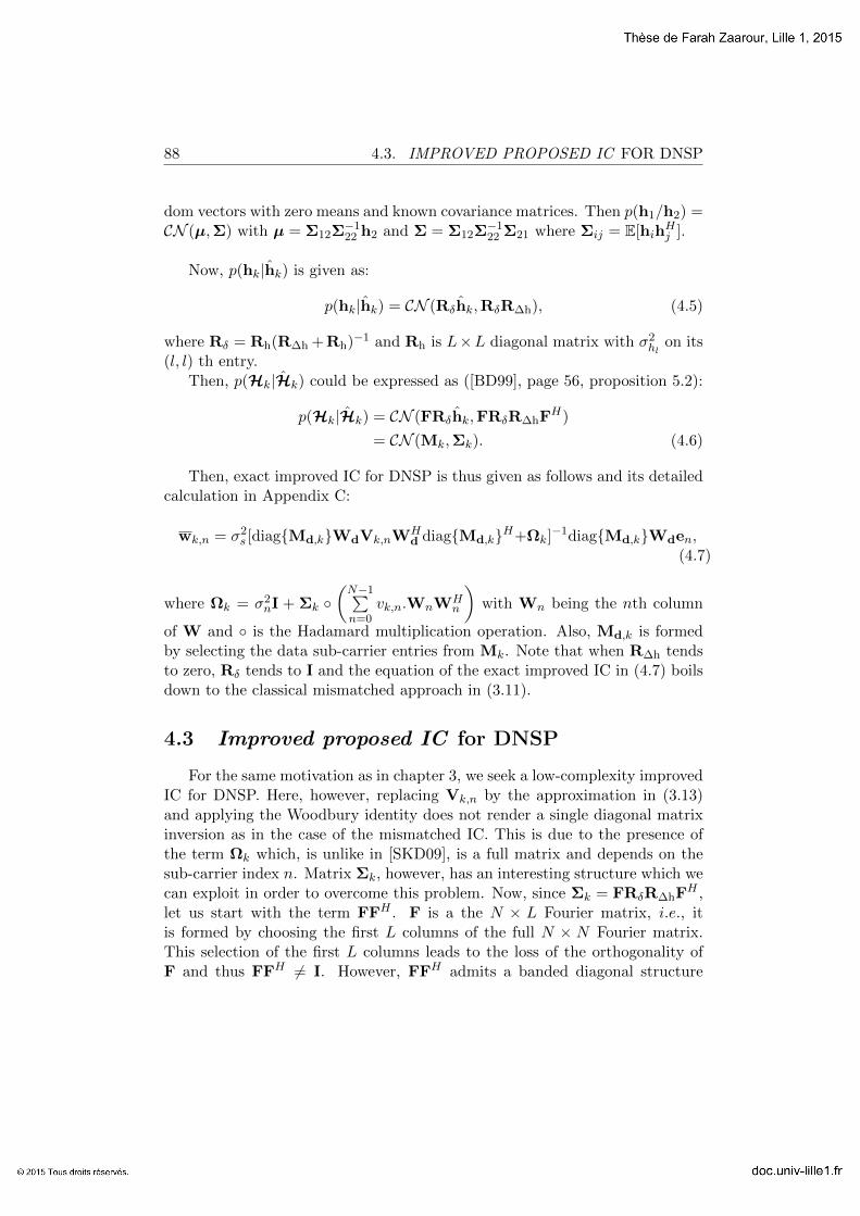
88 4.3. IMPROVED PROPOSED IC FOR DNSP
dom vectors with zero means and known covariance matrices. Then p(h1/h2) =CN (µ,Σ) with µ = Σ12Σ
−122 h2 and Σ = Σ12Σ
−122 Σ21 where Σij = E[hih
Hj ].
Now, p(hk|hk) is given as:
p(hk|hk) = CN (Rδhk,RδR∆h), (4.5)
where Rδ = Rh(R∆h + Rh)−1 and Rh is L×L diagonal matrix with σ2hl
on its(l, l) th entry.
Then, p(Hk|Hk) could be expressed as ([BD99], page 56, proposition 5.2):
p(Hk|Hk) = CN (FRδhk,FRδR∆hFH)
= CN (Mk,Σk). (4.6)
Then, exact improved IC for DNSP is thus given as follows and its detailedcalculation in Appendix C:
wk,n = σ2s [diagMd,kWdVk,nW
Hd diagMd,kH+Ωk]
−1diagMd,kWden,(4.7)
where Ωk = σ2nI + Σk
(N−1∑n=0
vk,n.WnWHn
)with Wn being the nth column
of W and is the Hadamard multiplication operation. Also, Md,k is formedby selecting the data sub-carrier entries from Mk. Note that when R∆h tendsto zero, Rδ tends to I and the equation of the exact improved IC in (4.7) boilsdown to the classical mismatched approach in (3.11).
4.3 Improved proposed IC for DNSP
For the same motivation as in chapter 3, we seek a low-complexity improvedIC for DNSP. Here, however, replacing Vk,n by the approximation in (3.13)and applying the Woodbury identity does not render a single diagonal matrixinversion as in the case of the mismatched IC. This is due to the presence ofthe term Ωk which, is unlike in [SKD09], is a full matrix and depends on thesub-carrier index n. Matrix Σk, however, has an interesting structure which wecan exploit in order to overcome this problem. Now, since Σk = FRδR∆hFH ,let us start with the term FFH . F is a the N × L Fourier matrix, i.e., itis formed by choosing the first L columns of the full N × N Fourier matrix.This selection of the first L columns leads to the loss of the orthogonality ofF and thus FFH 6= I. However, FFH admits a banded diagonal structure

CHAPTER 4. A LOW COMPLEXITY TURBO RECEIVER FOR DNSPIN OFDM WITH CHANNEL ESTIMATION ERRORS 89
0 2 4 6 8 10
10−4
10−3
10−2
10−1
100
SNR (dB)
BE
R
Mismatched exact IC
Mismatched proposed IC
Improved exact IC
Improved proposed IC
CSI
Figure 4.2: BER performance of the sixth iteration for 4QAM, K = 2, L = 15dB, Lf = 8 for mismatched exact IC, mismatched proposed IC, improved exactIC, improved proposed IC and CSI
which decreases with L and tends towards I. We show in figure 4.1 a typicalbehavior of FFH for different values of L. Now, the lth entry of the L × Ldiagonal matrix RδR∆h is
σ2hl
σ2nP
+σ2hl
σ2nP . The value of σ2
n decreases with SNR
and the entries of RδR∆h tends to a unique value proportional to σ2n and thus
the behavior of Σk becomes equivalent to that of FFH . Thus, we can see thatit is safe to ignore the off-diagonal entries of Σk as L increases and the SNRdecreases. We will later show by simulations that this assumption does notincur any performance degradation on the proposed IC while allowing us todesign a low-complexity IC.
Now, we can proceed as in chapter 3 to derive the approximated improvedIC by replacing Vk,n by the approximation in (3.13). Then, the improvedapproximated IC is given equivalently as in (3.17) as:
wk,n = λk,nwk,n, (4.8)
with:wk,n = σ2
s [Md,k(σ2s − σ2
s)MHd,k + (σ2
n + σ2a)I]−1Md,kWden, (4.9)

90 4.4. IMPROVED APPROXIMATED IC OF [?]
0 5 10 15 20
10−4
10−3
10−2
10−1
100
SNR (dB)
BE
R
Mismatched exact IC
Improved exact IC
CSI
Figure 4.3: BER performance of the sixth iteration for 16QAM, K = 3, L = 15dB, Lf = 8 for mismatched exact IC, improved exact IC and CSI
where σ2a = Tr(RδR∆h) · (σ2
s−σ2s)N+σ2
sN and
λk,n =σ2s
σ2s + σ2
seTnWH
d MHd,kwk,n
. (4.10)
4.4 Improved Approximated IC of [SKD09]
We review in this section an approximated version of the improved IC pro-posed in [SKD09]. The idea behind this approximation is to assume perfectsymbol estimation after the second iteration, i.e., vk,q = 0 for all q 6= n andvk,n = σ2
s . Let us first define A = diagMd,kWd and An being the nthcolumn of A, then the approximated IC of [SKD09] for DNSP is formulatedas:
wk,n = σ2s [Anσ
2sA
Hn + (σ2
n + σ2a)I]−1An,
=σ2sA
Hn
σ2sA
Hn An + (σ2
n + σ2a)
(4.11)

CHAPTER 4. A LOW COMPLEXITY TURBO RECEIVER FOR DNSPIN OFDM WITH CHANNEL ESTIMATION ERRORS 91
0 5 10 15 20
10−4
10−3
10−2
10−1
100
SNR (dB)
BE
R
Mismatched proposed IC
Improved proposed IC
CSI
Figure 4.4: BER performance of the sixth iteration for 16QAM, K = 3, L = 15dB, Lf = 8 for mismatched proposed IC, improved proposed IC and CSI
and σ2a = σ2
sTr(RδR∆h)N . We will refer to this IC as the improved IC of [SKD09].
4.5 Simulation results and discussions
For the simulations in this chapter, we use the same parameters as in chapter3 with a quasi-static channel. We first plot in figure 4.2, the BER performanceof the sixth iteration, i.e., at convergence, for a 4QAM modulation with L =15, Lf = 8 for the mismatched exact IC, the mismatched proposed IC, theimproved exact IC and the improved proposed IC. Note that the increase inthe number of channel paths renders the channel estimation harder. We cansee that the loss due to the approximation in both, the improved and themismatched case, is negligible. This is in accordance with the results in chapter3 for a 4QAM modulation. The gain from using the improved ICs at a targetBER of 10−5 is around 1 dB. We then plot in figure 4.3, the BER performance ofthe mismatched exact IC and the improved exact IC for a 16QAM modulation.Here, at a target BER of 10−5, the loss from themismatched exact IC withrespect to the improved optimal IC is negligible. This could be explained thatwith the increase of SNR, the effect of the channel estimation error decreases
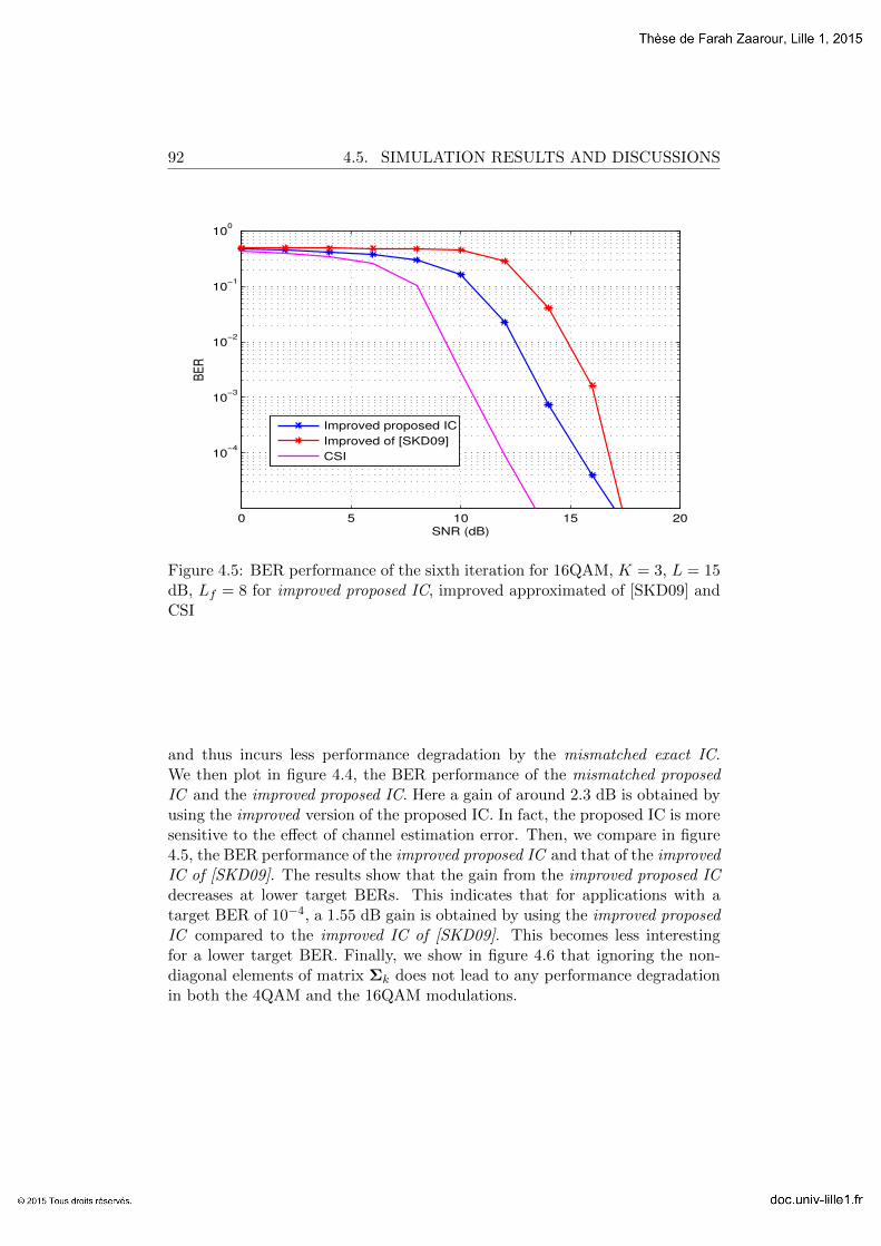
92 4.5. SIMULATION RESULTS AND DISCUSSIONS
0 5 10 15 20
10−4
10−3
10−2
10−1
100
SNR (dB)
BE
R
Improved proposed IC
Improved of [SKD09]
CSI
Figure 4.5: BER performance of the sixth iteration for 16QAM, K = 3, L = 15dB, Lf = 8 for improved proposed IC, improved approximated of [SKD09] andCSI
and thus incurs less performance degradation by the mismatched exact IC.We then plot in figure 4.4, the BER performance of the mismatched proposedIC and the improved proposed IC. Here a gain of around 2.3 dB is obtained byusing the improved version of the proposed IC. In fact, the proposed IC is moresensitive to the effect of channel estimation error. Then, we compare in figure4.5, the BER performance of the improved proposed IC and that of the improvedIC of [SKD09]. The results show that the gain from the improved proposed ICdecreases at lower target BERs. This indicates that for applications with atarget BER of 10−4, a 1.55 dB gain is obtained by using the improved proposedIC compared to the improved IC of [SKD09]. This becomes less interestingfor a lower target BER. Finally, we show in figure 4.6 that ignoring the non-diagonal elements of matrix Σk does not lead to any performance degradationin both the 4QAM and the 16QAM modulations.

CHAPTER 4. A LOW COMPLEXITY TURBO RECEIVER FOR DNSPIN OFDM WITH CHANNEL ESTIMATION ERRORS 93
0 5 10 15 2010
−4
10−3
10−2
10−1
100
SNR (dB)
BE
R
(b)
full
diag
0 2 4 6 810
−4
10−3
10−2
10−1
100
SNR (dB)
BE
R(a)
full
diag
Figure 4.6: BER performance of the sixth iteration for the improved proposedIC using Σk denoted full and by using only the diagonal elements of Σk denoteddiag (a) 4QAM (b) 16QAM
4.6 Conclusion
In this chapter, we extended the proposed IC of chapter 3 to include thechannel estimation errors. We showed that the gain from using the improvedproposed IC is more than 2 dB in a 16QAM modulation compared to 1 dB ina 4QAM modulation for a target BER of 10−5. This is since the proposed ICis more sensitive to channel estimation errors in a 16QAM modulation. Thoseresults lead us to the conclusion that the improved proposed IC is a goodcompromise between the complexity of the optimal ICs on the one hand andthe performance loss due to neglecting the channel estimation errors on theother hand.

Chapter5Perspectives: On Robust Estimationwith bounded data uncertainties
Contents
5.1 Introduction and Motivation . . . . . . . . . . . . . . 94
5.2 The regularized LS and its robust counterpart . . . 95
5.3 The Kalman filter and its robust counterpart . . . 97
5.4 Ambiguities associated with the robust approach . 102
5.5 Conclusion . . . . . . . . . . . . . . . . . . . . . . . . 103
5.1 Introduction and Motivation
In the previous chapters we have seen that the presence of uncertain in-formation at the OFDM receiver leads to the failure of conventional channelestimation algorithms. In particular, in the presence of NBI in chapter 2, theperformance of the Kalman filter deteriorates since the noise variance is un-known. The interference in classical superimposed pilots led to the failure of theLS estimator in chapter 2 since a portion of the power had been attributed tothe unknown data. This necessitated the design of more elaborate techniquesto overcome those problems. In fact, this behavior of the conventional channelestimators is explained by the fact that, by design, they require the knowledgeof certain underlying parameters. This knowledge varies from one estimator toanother and it depends on its nature. The LS estimator for example requiresthe knowledge of the observation matrix. The Kalman filter necessitates, in
94

CHAPTER 5. PERSPECTIVES: ON ROBUST ESTIMATION WITHBOUNDED DATA UNCERTAINTIES 95
addition to the observation matrix, the formulation of a state equation with aknown state matrix and the presence of the state and observation noise char-acteristics.
In this chapter, we investigate a different approach than those presentedin the previous chapters, which aims at dealing with the interference as modeluncertainties in the estimator’s design. Our aim is to shed the light on thepotentials and the underlying challenges of a bounded data uncertainty (BDU)class of robust estimators [SN99][Say01][SC02]. We also give insights abouttheir applications to problems in OFDM with interference. We will refer tothe BDU class as the robust approach. We note that the robust approach isa min-max approach where one aims at minimizing the cost function for theworst possible case.
This chapter is divided as follows. In sections 5.2 and 5.3, we briefly reviewthe work by Sayed on the robust approach for the regularized LS in 5.2 andthe Kalman filter in 5.3. In section 5.4, we provide our understanding on thisapproach and raise some questions and cast doubts on some assumptions relatedto the robust approach. Our goal is to try to get answers and give perspectivesfor future research directions. Finally, we conclude this chapter in section 5.5.
5.2 The regularized LS and its robust counterpart
The problem of ill-conditioned matrices which may arise in LS could beovercome by using the regularized LS (RLS). To understand the motivationbehind this approach, let us consider the following linear model:
b = Ax + v (5.1)
where b is the m× 1 observation vector, A, the m× n observation matrix,x, the n × 1 vector and v, the m × 1 noise vector. Note that in this chapter,we use the notations in [SN99]. The cost function of the RLS is formulated as:
J(x) = xHQx + (Ax− b)HR(Ax− b), (5.2)
where Q and R are symmetric known matrices chosen by the user for regular-ization purposes. They might represent, for example, the covariance matricesof x and v respectively. The solution to this problem is obtained by minimizingthe cost function in (5.2) and is given as:
x = [Q + AHRA]−1AHRb. (5.3)

96 5.2. THE REGULARIZED LS AND ITS ROBUST COUNTERPART
Note that for Q = 0 and R = I, the formulation in (5.3) boils down tothe conventional LS solution. This equation clearly reveals that the solutionnecessitates the knowledge of A, b.
Now, as per our discussion in section 5.1, only a partial knowledge of Aand b is guaranteed. In this case, it is clear to see that if the deviation of Aand b from their actual values is large, the solution x will lead to a high errorvariance since it will be far from x. This motivated the introduction of a newcost function to include the possible uncertainties [Say01][SN99] as:
J(x,u) = xHQx + (Ax− b + Tu)HR(Ax− b + Tu). (5.4)
Now, the formulation of the cost function in (5.4) depends on two unknowns;x which is to be estimated and a new variable u which is the unknown per-turbation vector. Comparing (5.2) and (5.4), we can see that the possibleuncertainties in A and b are modeled in the term Tu. The known matrixT allows the designer to choose a certain range space for the perturbation u.While u is unknown, yet a bound on its norm is assumed to be known, i.e.u ≤ φ(x). Then the min-max robust solution of x is given as:
x = arg minx
max‖u‖≤φ(x)
J(x,u). (5.5)
The formulation in (5.5) could be viewed as a two-player game where thedesigner tries to obtain the minimum x for the worst possible case of u.
In order to be able to concretely understand the formulation in (5.5), wewill consider a special case of uncertainties referred to as the structured uncer-tainties. If we define δA and δb as the unknown portions of A and b, thenin the structured uncertainties case, it is assumed that δA and δb satisfy thefollowing model:
[δA δb] = T∆[Ea Eb], (5.6)
where Ea and Eb are known values which depend on the given problem, and ∆is any contraction matrix, i.e.‖∆‖≤ 1, in which the uncertainties are modeled.In other words, for a given problem, if a designer is able to model the uncer-tainties in A and b as the model in (5.6), then he should be able to formulatea robust solution to the problem.
Now, due to the unknown portions of A and b, we can replace A and b in(5.2) by A + δA and b + δb respectively. Then, (5.4) could be re-written as:
J(x,u) = xHQx + (Ax− b + (δAx− δb))HR(Ax− b + (δAx− δb)), (5.7)

CHAPTER 5. PERSPECTIVES: ON ROBUST ESTIMATION WITHBOUNDED DATA UNCERTAINTIES 97
and with Tu = (δAx − δb) = T(∆Eax − Eb), then u is defined as u =∆(Eax−Eb).
Then, after solving (5.5) which as we will see, conserves the structure ofits conventional counterpart, where only the weighing matrices (W and R) arereplaced by their corrected versions (W and R), the robust solution to (5.7) isgiven as [SN99][Say01]:
x = [Q + AHRA]−1AHQb. (5.8)
where Q and R are given as:
Q = Q + λEHa Ea; R = R + RT(λI−THRT)†THR. (5.9)
We can see from (5.9) that in order to obtain the corrected weighing matrices(Q and R), a scalar λ is to be determined. This is obtained through a numericaloptimization problem as the minimum of a certain non-linear function G(λ) as:
λ = arg minλ≥‖THRT‖
G(λ), (5.10)
with G(λ) defined as:
G(λ) = ‖x(λ)‖2Q(λ)+λ‖Eax(λ)−Eb‖2+‖Ax(λ)− b‖2R(λ) (5.11)
with:
R(λ) = R + RT(λI−THRT)†THR (5.12)
Q(λ) = Q + λEHa Ea (5.13)
x(λ) = [Q(λ) + AHR(λ)A]−1[AHR(λ)b + λEHa Eb]. (5.14)
5.3 The Kalman filter and its robust counterpart
When the parameter to be estimated evolves with time according to a dy-namical model, it becomes more reasonable to resort to the Kalman filter ratherthan to the RLS to perform estimation. The implementation of the Kalmanfilter requires, in addition to the observation equation, a state equation. The

98 5.3. THE KALMAN FILTER AND ITS ROBUST COUNTERPART
100
101
102
103
0
5
10
15
20
25
i
Err
or
Va
ria
nce
(d
B)
Optimal
Kalman
Robust
Figure 5.1: Error variance of three filters with ∆i selected uniformly within theinterval [-1,1], T(1)=0.0198, F(1,2)=0.0196
set of those two equations is known as the state space equations and is givenas:
xi+1 = Fxi + wi (5.15)
bi = Axi + vi (5.16)
where (5.15) is the state equation and (5.16) is the observation equationwith F being the state matrix, G, the covariance matrix of the state noise wi,A, the observation matrix, R, the variance of the observation noise vi and Qthe covariance matrix of xi.
The Kalman filter estimates a process by using a form of feedback control.The filter estimates the process state at some time and then obtains feedbackin the form of noisy measurements. This is done via the measurement and timeupdate equations. In fact, those equations admit a deterministic interpretationas a solution to a RLS problem [Say01]. In other words, the measurement up-date and the time update equations of the Kalman filter could be derived by

CHAPTER 5. PERSPECTIVES: ON ROBUST ESTIMATION WITHBOUNDED DATA UNCERTAINTIES 99
100
101
102
103
0
5
10
15
20
25
30
35
40
i
Err
or
Va
ria
nce
(d
B)
Optimal
Kalman
Robust
Figure 5.2: Error variance of three filters with ∆i selected uniformly within theinterval [-1,1], T(1)=0.198, F(1,2)=0.0196
posing a regularized least-squares problem and imposing some identifications.We give the details of this derivation in Appendix D. In fact, this allowed theauthor in [Say01] to extend the robust solution presented in section 5.2 for RLSto the robust Kalamn filter. The detailed formulations of the different forms ofthe robust Kalman filter could be found in [Say01].
In this section, our goal is to show the relative performance of the robustKalman filter and its classical counterpart. We do that with a numerical exam-ple used in [Say01] to motivate the interest of the robust Kalman filter. Thisnumerical example is also widely use in robust problems [PS99]. We will firstrecall the results provided by Sayed where he showed that by considering astructured uncertainty in the state matrix constructed as in (5.6), the steady-state performance of the robust Kalman filter in terms of the error variance isbetter than that of the Kalman filter.
Consider now the following state-space model with uncertainties:

100 5.3. THE KALMAN FILTER AND ITS ROBUST COUNTERPART
100
101
102
103
0
2
4
6
8
10
12
14
i
Err
or
Va
ria
nce
(d
B)
Optimal
Kalman
Robust
Figure 5.3: Error variance of three filters with ∆i selected uniformly within theinterval [-1,1], T(1)=0.0198, F(1,2)=0.3912
xi+1 = (F + T∆iEf )xi + wi (5.17)
bi = Axi + vi (5.18)
Here, Ef and T represent the known parameters of the uncertainty givenin (5.6). Notice also the dependence of ∆i on the time index i. Let us nowconsider the numerical example of [Say01]:
F =
[0.9802 0.0196
0 0.9802
]; G =
[1 00 1
];
A =[1 −1
]; T =
[0.0198
0
]; R = 1
Ef =[0 5
]; Q =
[1.9608 0.01950.0195 1.9605
];

CHAPTER 5. PERSPECTIVES: ON ROBUST ESTIMATION WITHBOUNDED DATA UNCERTAINTIES 101
With this model, we have F at our disposal, whereas the actual state matrix(Fa = (F + T∆iEf )) is:
Fa =
[0.9802 0.0196 + 0.099∆i
0 0.9802
];
We plot the error variance of three filters; the Kalman filter with the knowl-edge of F which is referred to as Kalman in the figures, the robust Kalman filterreferred to as Robust, and the optimal Kalman filter referred to as Optimal.More precisely, the Kalman filter uses the underlying model as if it were theactual one, the robust Kalman filter takes the uncertainties into account whiledesigning the cost function of the estimator and the Optimal Kalman filter hasthe knowledge of the true matrix Fa. First, we plot in figure 5.1, the errorvariance performance of the three filters with ∆i selected uniformly within theinterval [-1,1] and with the given parameters. We can see that the error vari-ance of the robust filter is lower than that of the Kalman filter and closer tothe performance of the optimal filter. The performance loss is around 2.5 dBat steady-state. The degradation in the performance of the Kalman filter is ex-plained by the fact that it has been formulated with an erroneous model. Next,we keep the same parameters as for figure 5.1 and only change T(1) = 0.198.T here represents the uncertainty in the model and increasing its value mightbe viewed as increasing the uncertainty in the system. We regenerate the sameplots of figure 5.1 in figure 5.2. The results show that the performance degrada-tion of the Kalman filter is more important than in the previous configurationand reaches around 17 dB at steady-state. This indicates that as the uncer-tainty in the model increases, the performance degradation of the Kalman filterwith respect to both the optimal and the robust filter increases. Those two fig-ures have been exposed in [Say01] to show the interest of the robust approach.While those results might be very promising, more recent work on this topic[XM09], showed that through this same numerical example, changing a param-eter in the system matrix, renders the performance of the robust filter worsethan the Kalman filter. We regenerate this example in figure 5.3 where theinitial parameters are kept the same while replacing the (1,2)th entry of F by0.3912. F represents the certainty in the system and increasing its value meansincreasing the certainty in the system. The figure shows that the performanceof the robust Kalman filter deteriorates considerably and that of the Kalmanfilter approaches the performance of the optimal filter.
Those results are explained by the authors in [XM09] as the results of theconservative nature of the robust approach. In other words, they explain that

1025.4. AMBIGUITIES ASSOCIATED WITH THE ROBUST APPROACH
this change in the state matrix decreased the uncertainty and under such con-ditions, the robust approach becomes pessimistic and performs worse than theconventional filter. However, the authors do not precise how the robust ap-proach is conservative.
We finally note that for obtaining parameter λ, the authors in [Say01] as-sume that the function G(λ) tends to reach amplitudes close to its minimumvalue at arguments of λ close to its lower bound (λl = ‖THRT‖). They con-sequently propose a practical approximation for λ as λ = (1 + α)λl.
5.4 Ambiguities associated with the robust approach
We reserve this section for some ambiguous points associated with the ro-bust approach. First, the results in section 5.3 suggests that this approach isefficient only under certain uncertainty conditions. In particular, the authors in[XM09] argue that the robust approach outperforms the conventional approachonly when a high uncertainty is present in the system. They further relate thisfact to the conservative nature of the robust approach.
6 7 8 9 10 11 1215
20
25
30
35
40
45
50
55
λ
G(λ
)
min
(a) G(λ) in interval [λl, 12] ,
0 2 4 6 8 10 12−300
−200
−100
0
100
200
300
λ
G(λ
)
(b) G(λ) in interval [0, 12]
Figure 5.4: G(λ)
It would be interesting to investigate a theoretical framework that enablesthe designer to determine the uncertainty for a given problem.
The second point which is not thoroughly justified for the implementationof the robust approach is the choice of the parameter λ. We will first considera numerical example provided by the authors in [SC02] and plot the function

CHAPTER 5. PERSPECTIVES: ON ROBUST ESTIMATION WITHBOUNDED DATA UNCERTAINTIES 103
G(λ).
Given the following parameters:
A =
1 −10 1−2 00 2
; b =
−101−2
; Q =
[1 00 2
];
Ea =
1 00 −21 10 0
; R = 1; Eb =
1001
; T =
−1 01 20 01 −1
;
we have λl = ‖THRT‖= 5.4142. We plot the G function for this prob-lem for the interval [λl, 12] in figure 5.4a and for the interval [0, 12] in figure5.4b. We notice that the minimum of G(λ) within the interval [λl,∞[ is λlitself. We notice that an important point (the lower bound of the interval) hasbeen neglected by the authors. Although, the authors show in [Say01] thatthe approximation of this parameter has no effect on the performance of thealgorithm, nevertheless, if we closely look into (5.8), we can see that in casethe true λ lies on the lower bound, then the robust solution boils down to theconventional RLS solution with a new regularization parameter Q.
It would be also interesting to investigate this point in more details tounderstand its effect on the solution to the robust problem.
5.5 Conclusion
In this chapter, we reviewed a min-max robust approach which takes intoaccount the model uncertainties in the design of the estimator. The attractiveaspect of this approach is that it conserves the structure of its conventionalcounterparts. We have then recalled the state of the art and presented a nu-merical example which has been used by the authors in literature to motivatefor this approach. This example shows the interesting potential of the robustapproach, but also its conservative nature. We have raised some concerns re-garding this approach which are open questions that provide an interestingperspective in this field. One very interesting framework to apply the robustapproach to is the turbo reception framework. In fact, the uncertainties present

104 5.5. CONCLUSION
in turbo estimation due to the symbol estimation error is unknown but couldbe bounded. This can be done by making use of the variance of the symbolestimation error provided at each turbo iteration.
General conclusion and perspectives
A high quality channel estimation at the OFDM receiver should be main-tained throughout the communication interval, so as to guarantee an acceptablesystem performance with the ultimate goal of coherent data detection. Whiledesigning channel estimation algorithms, a reasonable balance should be estab-lished between the system performance and the receiver’s complexity on theone hand, as well as a trade-off is to be considered between the quality of thechannel estimate and the spectral efficiency of the system on the other hand.In other words, a compromise should be done so as to maximize the spectralefficiency and reduce the complexity while maintaining an acceptable channelestimation performance. Those three criteria form the road map of our thesis.
Channel estimation in OFDM is often accomplished by inserting knownpilot symbols within the OFDM frame. This is known as the pilot-symbol as-sisted modulation (PSAM). In order to be able to apply conventional channelestimation algorithms (LS, MMSE, ...) to those systems, a minimum number ofpilots should be inserted with a minimal interference level. The first constraintwhich is the number of pilots, means that valuable bandwidth which couldhave been attributed to data is to be sacrificed. Consequently, this decreasesthe data rate which is in an ever-increasing demand. The second constraint ofinterference-free pilots can not be always met and interference could originatefrom different sources. A solution to the first problem has been envisioned. Itaims at replacing conventional pilots (PSAM scheme) by superimposed pilots(SP). SP do not require a dedicated bandwidth, however, their presence leadsto the rise in interference. In particular, we distinguish between two variantsof SP; the classical SP (CSP) and the data-nulling SP (DNSP). In CSP, theinterference arises from data on pilots in channel estimation and from pilots ondata in data detection. In DNSP, interference on data originates from nulling
105

106 GENERAL CONCLUSION AND PERSPECTIVES
data sub-carriers after precoding for the insertion of pilot sub-carriers. Thus,we can see that by addressing the first problem, the second problem is worsened.
In a different context, where the initial goal was to optimize the spectralefficiency, the cognitive radio (CR) environment imposes the co-existence oftechnologies in the same frequency band. This may generate interference andeven with PSAM, conventional channel estimation algorithms fail.
Thus, we dedicate this thesis to the design of channel estimation algorithmsfor OFDM systems in the presence of interference.
We organize this work in five chapters. Chapter one is dedicated to a briefintroduction of the radio channel and the basic OFDM system. We distinguishbetween two types of channels in OFDM; the quasi-static channel and the fasttime-varying channel. It is well known that in the case of high mobility, i.e. fasttime-varying channel, the orthogonality between the sub-carriers of the OFDMsystem and thus the channel estimation approaches designed for quasi-staticsystems differ from those designed for fast time-varying systems. Further, wedifferentiate between two kinds of interference; narrowband interference (NBI)which exists in cognitive radio (CR) networks and interference from SP as dis-cussed above.
In chapter two, we consider the problem of channel estimation in fast time-varying channels for OFDM systems contaminated by NBI. NBI strikes a smallnumber of sub-carriers with a high power and renders conventional channelestimation algorithms inefficient. For the first time, we propose a channel es-timation framework in this context. This has been done via the MAP EMalgorithm. The problem is formulated so as to elegantly integrate the Kalmansmoother for the estimation of the channel taps. We then simulate the pro-posed algorithm in a real world scenario and show its robustness to mobility interms of MSE and BER performance, in contrast to existing algorithms whichhave not been designed to handle mobility. In addition, this is obtained at thecost of a reasonable additional complexity.
In chapters three and four, we consider the problem of channel estimationand data detection in DNSP. DNSP is a recently proposed scheme for OFDMand the design of a dedicated receiver is yet to be addressed. Thus we pro-pose a receiver design for DNSP based on turbo reception. Turbo reception iswell-known to be the most efficient in interference cancellation. However, this

Conclusion 107
efficiency comes at the cost of high complexity and the necessity of a precisechannel estimate.
In chapter three, we deal with the complexity issue and propose a low-complexity receiver for DNSP by exploiting the special interference structurein this scheme. The receiver is based on the MMSE soft interference canceler(IC). Then, we initiate a performance comparison between DNSP with the pro-posed receiver and the CSP scheme in an iterative receiver. We first show thatan important gain in terms of BER is achieved by DNSP compared to classicalsuperimposed pilots (CSP) at the cost of a higher complexity. This is explainedby the increased transmission diversity due to the precoding, which is part ofthe DNSP design. We then show that a coded-CSP scheme is able to achievethe same BER performance as DNSP but this time at the cost of a higher com-plexity. From this study we conclude that increasing the transmission diversityin SP schemes is more profitable in terms of complexity via the DNSP scheme.
The performance of the proposed IC for DNSP in chapter three is onlyreliable when the channel estimation error is small. Although DNSP offersby design interference-free pilots, yet in some scenarios the channel estimatemight not be reliable. We thus design in chapter four an enhanced IC for DNSPwhich takes the channel estimation errors into account. The results show thatthe enhanced IC is particularly interesting in scenarios with a high channelestimation error. In addition, the gain in BER is more interesting in 16QAMwhich could reach up to 2.3 dB compared to 1 dB in 4QAM at a target BERof 10−5 since the IC is more sensitive to channel estimation errors for higherorder modulations. However, we should point out that in DNSP and unlike inPSAM, the increase in the number of pilots does not necessarily improve theBER since a higher number of pilots leads to more interference.
In the last chapter, we shed the light on a min-max robust approach. Wefirst expose the robust counterparts of the regularized least-squares and theKalman filter. We then present some interrogations about this approach andpresent a perspective for its possible application.
Finally, the work presented in this thesis has an interesting potential forfuture research:
• Perspectives on chapter two:
In chapter two, we used a Gaussian model for NBI. It would beinteresting to obtain more accurate models for NBI through measurement
108 GENERAL CONCLUSION AND PERSPECTIVES
campaigns. This will help give a clearer idea about the effect of this modelon the performance of the algorithm. In fact, a new channel sounder hasbeen designed at TELICE and which is planned to be used in futuremeasurement campaigns.
Despite the advantages of the OFDM system, which led to its stan-dardization in 4G systems, its documented drawbacks should be ad-dressed while choosing an appropriate modulation for 5G systems. Theuniversal filtered multi-carrier (UFMC) and the generalized frequencydivision multiplexing (GFDM) are the two serious candidates for 5G sys-tems. UFMC is very close in nature to OFDM and is referred to as theuniversal filtered OFDM (UF-OFDM) as well. Unlike filtered OFDMwhich applies a filter to each sub-carrier and filter bank based multi-carrier (FBMC) which applies a filter to the entire band, the UFMC ap-plies filters on a per band basis thus preserving the advantages of OFDMwhile reducing the effect of high spectral lobes in OFDM. This propertycould be very interesting in rendering the system more robust to inter-ference. GFDM is also a generalized form of OFDM. However, unlikeOFDM which uses one cyclic prefix (CP) per symbol, it uses only oneCP for a group of symbols. Recent studies point out that GFDM is wellsuited to cognitive radio (CR), since the rectangular pulse used in OFDMis replaced by a choice of pulse shaping. This lowers the side lobes in thefrequency domain. As a perspective, the study of the impact of NBI inUFMC and GFDM systems which are, by design, robust to interference,could further give insights about the advantage of one system to the otherfrom an interference point of view.
• Perspectives on chapters three and four:
In chapters 2 and three of this thesis, we saw the different variantsof superimposed pilot (SP) schemes proposed for OFDM so as to replacethe bandwidth-consuming conventional pilots. The channel estimationtask and pilot placement schemes are also important aspects to be stud-ied in UFMC and GFDM systems. UFMC, as already stated, preservesthe OFDM structure and thus the extension of the channel estimationand the pilot schemes to UFMC should be direct forward. However, inGFDM, since the data now is transmitted in the time domain and thenfrequency domain equalization (FDE) is performed at the receiver, thetransmitted data are mixed up, the insertion of conventional pilots asin OFDM becomes inefficient. The study of particular pilot schemes forGFDM is an interesting challenge and an open perspective. The work

Conclusion 109
presented in chapters 3 and 4 of this thesis could be the starting point ofthis work.
• Perspectives on chapter five:
The further research on robust channel estimators to problems ofchannel estimation with interference in OFDM is an open topic. Aninteresting area of research could be to consider uncertainties in the co-variance matrix of the channel noise rather than in the system matrices.This could be an interesting application to the environments with NBI.We note here that we have already considered the application of the H∞filter to the NBI problem. However, the results were disappointing al-though the H∞ filter is designed without restrictions on the distributionor the knowledge of the system’s noise. Another challenging aspect is toprovide a theoretical framework which explains the underlying function-ality of the robust approaches.
AppendixACalculations related to chapter two
A.1 Computation of the Q Function
In order to obtain the expression for Q(σ2, σ2(i)
), we take the expectation
with respect to c conditioned on y, given the current parameter estimate σ2(i)
.We have from (2.19):
Q(σ2, σ2(i)
) = −Kln∏
n
σ2n+
K−1∑
k=0
Tr
Ec|y,σ2
(i)
[(yk −X kck)
H C−1 (yk −X kck)]
(A.1)
From (A.1), we obtain:
Q(σ2, σ2(i)
) = Tr
C−1(ykyHk + X kS
(i)k|KXH
k −ykc(i)H
k|K XHk −X kc
(i)k|KyHk )
(A.2)
where S(i)k|K
def= E
c|y,σ2(i)
[ckc
Hk
]and c
(i)k|K
def= E
c|y,σ2(i) [ck]. Let us define:
P(i)k|K
def= E
c|y,σ2(i)
[(ck − c
(i)k|K)(ck − c
(i)k|K)H
]
= S(i)k|K − c
(i)k|K c
(i)H
k|K (A.3)
Then by substituting (D.23) into A.2, we obtain (2.23).
110

APPENDIX A. CALCULATIONS RELATED TO CHAPTER TWO 111
A.2 Calculation of σ2n
(i+1)
We provide here the calculation of σ2n
(i+1)in equation (2.24).
E-step:
σ2n
(i+1)= arg max
σ2n
Q(σ2, σ2(i)
) + ln p(σ2)
= −K ln
N−1∑
n=0
σ2n −
K−1∑
k=0
TrC−1(X kP
(i)k|KXH
k + (yk −X kc(i)k|K)(yk −X kc
(i)k|K)H
+ ln[λ
σ4n
exp−λσ2n
]
= −K lnN−1∑
n=0
σ2n −
K−1∑
k=0
TrC−1(X kP
(i)k|KXH
k + (yk −X kc(i)k|K)(yk −X kc
(i)k|K)H
+ lnλ− 2 lnσ2n −
λ
σ2n
M-step:
Now, we derive with respect σ2n and equate to zero.
Define Mk = (X kP(i)k|KXH
k + (yk −X kc(i)k|K)(yk −X kc
(i)k|K)H , we have:
−Kσ2n
−k=K−1∑
k=0
− 1
σ4n
[Mk]n,n −2
σ2n
+λ
σ4n
= 0
− K
−σ2n
− 2
σ2n
= −K−1∑
k=0
1
σ4n
[Mk][n, n]− λ
σ4n
K + 2 = σ2n
[K−1∑
k=0
1
σ4n
[Mk]n,n +λ
σ4n
]
K + 2 =
K−1∑
k=0
1
σ2n
[Mk]n,n +λ
σ2n
Then,
σ2n
(i+1)=
1
K + 2
K−1∑
k=0
[Mk]n,n +λ
K + 2(A.4)

112A.3. ADDITIONAL COMPLEXITY CALCULATION FOR PROPOSED
ALGORITHM WITH RESPECT TO ALGORITHM IN [?]
A.3 Additional complexity calculation for proposedalgorithm with respect to algorithm in [HR10]
In order to calculate the additional complexity required by the proposedalgorithm, we have to calculate:
σ2n
(i+1)=
1
K + 2︸ ︷︷ ︸O1
K−1∑
k=0︸︷︷︸O2
[Mk]n,n︸ ︷︷ ︸O3
+λ
K + 2︸ ︷︷ ︸O4
. (A.5)
and Mk = X kP(i)k/KXH
k︸ ︷︷ ︸O3c
+ (yk −X kc(i)k|K)
︸ ︷︷ ︸O3a
(yk −X kc(i)k|K)H
︸ ︷︷ ︸O3b
.
︸ ︷︷ ︸O3d
For calculating O1, 1 RM and 1 RA is required. O4 requires only 1 RM sincethe addition has been already done in O1. Now, for the calculation of O3 which
we divide into sub-operations, calculating Xkc(i)k|K in O3a needs NLNc CM and
N(LNc − 1) CA and then N CA for the subtraction from yk. Operation O3bresults in an N ×N Hermitian matrix. Thus the real diagonal entries will need2 RM and 1 RA each, and the non-diagonal entries will require N2 − N CM.However, we notice that for the calculation of (A.5), only the diagonal entriesof Mk are required and thus it is enough to compute only those entries. Thusthe complexity of this step is reduced to 2N RM and N RA. For operation
Table A.1: Additional Complexity of the proposed algorithm
Operation RA RM CA CM
O1 1 1 - -O2 N(K − 1) - - -O3a - - NLNc NLNc
O3b N 2N - -O3c - - NLN2
c −N NLN2c +NLNc
O3d N - - -O4 − 1 - -
Total NK +N + 1 2N + 2 NLN2c +NLNc −N NLN2
c + 2NLNc

APPENDIX A. CALCULATIONS RELATED TO CHAPTER TWO 113
O3c, NLN2c + NLNc CM and NLNc(Nc − 1) + N(LNc − 1) CA are needed
to compute the diagonal entries of O3c. O3d will thus require N RA since theaddition of the diagonal entries of O3b and O3c needs a single RA per sub-carrier. Then to finalize this calculation, operation O2 requires (K−1) RA foreach sub-carrier and thus a total of N(K− 1) RA. This is summarized in tableA.1.

AppendixBCalculations related to chapter three
B.1 Demonstration of equation (3.17) from (3.11)
wk,n = σ2s [Gd,kVk,nG
Hd,k + σ2
nI]−1Gd,ken, (B.1)
Now using the approximation (3.13), Vk,n becomes:
Vk,n =
σ2s − σ2
s 0 . . . . . . 0...
. . .... σ2
s...
. . .
0 σ2s − σ2
s
Then (B.1) can be re-written as:
wk,n = σ2s(Gd,k[(σ
2s − σ2
s) I + σ2sene
Tn ]GH
d,k + σ2nI)−1Gd,ken. (B.2)
By using Woodbury identity defined as:
(A + uvH)−1 = A−1 − A−1uvHA−1
1 + vHA−1u(B.3)
where A = diagHd,k(σ2s − σ2
s)diagHd,kH + σ2nI, u = σ2
sdiagHd,kWdenand vH = eTnWH
d diagHd,kH , we have:
wk,n = σ2s
[A−1 − A−1uvHA−1
1 + vHA−1u
]Gd,ken. (B.4)
114

APPENDIX B. CALCULATIONS RELATED TO CHAPTER THREE 115
Since A is hermitian and u = σ2sv, then (B.4) can be written as:
wk,n = σ2s
[A−1Gd,ken
1 + σ2seTnGH
d,kA−1Gden
]Gd,ken. (B.5)
Now, defining wk,n = σ2sA−1Gd,ken, then (B.5) becomes:
wk,n = σ2swk,n
σ2s + σ2
seTnGH
d,kwk,n
, (B.6)
which could be written as:
wk,n = λk,nwk,n, (B.7)
where λk,n
λk,n =σ2s
σ2s + σ2
seTnWH
d diagHd,kHwk,n
. (B.8)
The only matrix inversion required now is A−1 and which is a diagonalmatrix inversion due to the property of W (WdWH
d = I).
B.2 Complexity Computation of the mismatched ex-act IC and the mismatched proposed IC
We detail here the given complexities of the three ICs given in Table 3.1.We first note that a CM is equivalent to 4 RM and 2 RA and a CA is equivalentto 2 RA.
B.2.1 Complexity of mismatched exact IC
Define O1 = diagHd,kWd, then the equalization vector for the optimalIC is given as:
wk,n =
O5︷ ︸︸ ︷σ2s [O1Vk,nO1H︸ ︷︷ ︸
O2
+σ2nI
︸ ︷︷ ︸O3
]−1
︸ ︷︷ ︸O4
O1en (B.9)
To accomplish operation O1, we need 2ND RM. Its Hermitian has no addi-tional complexity. O2 results in a D×D matrix. The calculation of its diagonal
116B.2. COMPLEXITY COMPUTATION OF THE MISMATCHED EXACT
IC AND THE MISMATCHED PROPOSED IC
entries require 3 RM and 1 RA each, thus a total of 3D RM + (2D − 1) RA,its D2 −D non diagonal entries need 1 CM, 2 RM and (D − 1) CA each, thusa total of (D2 − D)(1 CM + 2 RM + (D − 1) CA). O3 and O4 need D RAand D3 CM respectively. Operation O5 could be written as: σ2
sO4O1As whereO1As = O1AenO1As. O1As is a selection operation and does not add to thecomplexity. O4 O1As results in a D × 1 vector which needs D CM and (D-1) CA per entry and thus a total of D(D CM + (D − 1) CA), finally themultiplication with σ2
s needs 2D RM.
Now the filtering operation is given as follows:
sk,n =
O6C︷ ︸︸ ︷wk,n
H (yd,k −O1Bsk)︸ ︷︷ ︸O6A︸ ︷︷ ︸
O6B
(B.10)
O6A results in a D × 1 vector and each entry needs N CM and (N − 1) CA,thus a total of D(N CM + (N − 1) CA), D CA for O6B. O6C results in ascalar with D CM + (D − 1) CA.
B.2.2 Complexity of mismatched proposed IC
The equalization vector for the proposed IC is given as:
wk,n = σ2s
O4︷ ︸︸ ︷[diagHd,k(σ2
s − σ2s)diagHd,kH︸ ︷︷ ︸
O2
+σ2nI
︸ ︷︷ ︸O3
]−1O1en
︸ ︷︷ ︸O6
(B.11)
First, O1 = diagHd,kWd needs 2ND RM. To accomplish operation O2which results in a D × D real diagonal matrix, we need 3 RM and 1 RA foreach entry, for a total of D(3 RM+1 RA). O3 is the addition of 2 real diagonalmatrices and thus needs D RA. Finally, operation O6 could be written as: σ2
s
O4 O1 en, O1 en is a selection operation. O4 O1 en is the multiplication ofa real diagonal matrix and a complex vector which results in a D × 1 vectorand needs 2 RM per entry so 2D RM in total. The last operation which is themultiplication by σ2
s also requires 2D RM.

APPENDIX B. CALCULATIONS RELATED TO CHAPTER THREE 117
O7 = λk =
O7D︷ ︸︸ ︷σ2s
σ2s + σ2
s eTnWHd diagHkd,kHwk,n︸ ︷︷ ︸
O7A︸ ︷︷ ︸O7B︸ ︷︷ ︸
O7C
(B.12)
O7A is the selection of the (n,n) entry of an N ×N matrix and needs 3 RM +1 RA, O7B needs 1 RM, O7C 1 RA and O7D 1 RM.
Now the filtering operation is given as:
sk,n =
O8D︷ ︸︸ ︷
λkwk,n︸ ︷︷ ︸O8C
O8B︷ ︸︸ ︷(yd − diagHd,kWdsk)︸ ︷︷ ︸
O8A
O8A results in a D × 1 vector which needs D(N CM + (N − 1) CA), O8Bneeds D CA, O8C needs 2D RM, and O8D results in a scalar that necessitatesD CM + (D − 1) CA.

AppendixCCalculations related to chapter four
We demonstrate here the derivation of the improved IC for DNSP.The channel impulse response hk, the covariance matrix Rh of hk and the
covariance matrix of the LS channel estimation error R∆h ar given as:
hk =
h0...
hL−1
; hk =
h0...
hL−1
Rh
σ2h0
. . .
σ2hL−1
; R∆h =
σ2nP
. . .σ2nP
Then:p(hk|hk) = CN (Rδhk,RδR∆h), (C.1)
where Rδ = Rh(R∆h + Rh)−1 [SKD09].
Now, p(Hk|Hk) could be expressed as ([BD99], page 56, proposition 5.2):
p(Hk|Hk) = CN (FRδhk,FRδR∆hFH)
= CN (Mk,Σk). (C.2)
. Let us recall the equation of the exact mismatched IC for DNSP as:
wk,n = σ2s [Gd,kVk,nG
Hd,k + σ2
nI]︸ ︷︷ ︸
Ry
−1Gd,ken︸ ︷︷ ︸
Ry,s
. (C.3)
118

APPENDIX C. CALCULATIONS RELATED TO CHAPTER FOUR 119
Now, the improved approximated IC is calculated as:
wk,n = σ2sR−1y Ry,s, (C.4)
where Ry = EHk|HkRy and Ry,s = EHk|Hk
Ry,s.
Now, we need to calculate EHk|HkGd,kVk,nG
Hd,k and EHk|Hk
Gd,ken.
EHk|HkGd,kVk,nG
Hd,k = EHk|Hk
N−1∑
n=0
vngngHn
(C.5)
=N−1∑
n=0
EHk|Hk
vngngHn
(C.6)
where gn is the nth column of matrix Gd,k where we drop the index k tosimplify notations.
EHk|HkvngngHn = vnEHk|Hk
gngHn (C.7)
andEHk|Hk
gngHn = AnAHn + (Σk Wn). (C.8)
where A = diagMd,kWd, Wn is the nth column of Wd and is theHadamard multiplication operation.
Then,
EHk|HkGd,kVk,nG
Hd,k = AVk,nA
H + Σk (N−1∑
n=0
vnWnWHn
). (C.9)
And,EHk|Hk
Gd,ken = Aen. (C.10)
Finally, replacing (C.9) and (C.10) into (C.4), we obtain the formulation of theexact improved IC for DNSP.
We still have the approximated improved IC for DNSP which is derivedfollowing the same procedure as in Appendix B.

AppendixDCalculations related to chapter 5
Consider the following state-space model at instant i:
xi+1 = Fixi + Giwi (D.1)
bi = Aixi + vi (D.2)
We also define the following matrix identities which will be useful in our deriva-tion:
(A + BDC)−1 = A−1 −A−1B(D−1 + CA−1B)−1CA−1 (D.3)
DC(A + BDC)−1 = (D−1 + CA−1B)−1CA−1 (D.4)
(A + UCV)−1 = A−1U(C−1 + VA−1U)−1VA−1 (D.5)
Then after receiving a new measurement bi+1, xi is estimated by solvingthe following equation by minimizing with respect to xi and xi+1:
J = minxi,wi
[‖xi − xi/i‖2Pi/i−1+‖wi‖2Qi−1+‖bi+1 −Ai+1xi+1‖2Ri+1
−1 ]. (D.6)
We have that the differential of a quadratic form is given by:
d(xTQ−1x) = d(xT )Q−1x + xTQ−1d(x) = 2d(xT )Q−1x (D.7)
Then, derivatives of J w.r.t xi and xi+1 are respectively given as:
dJxi
= −P−1i/i (xi/i − xi)− FT
i Q−1i (xi+1 − Fixi), (D.8)
120

APPENDIX D. CALCULATIONS RELATED TO CHAPTER 5 121
dJxi+1
= Q−1i (xi+1 − Fixi)−AT
i+1R−1i+1(bi+1 −Ai+1xi+1) (D.9)
Now, by equating (D.8) and (D.9) to zero, we obtain the following system ofequations:
(P−1i/i + FT
i Q−1i Fi)xi = P−1
i/i xi/i + FTi Q−1
i xi+1, (D.10)
(ATi+1R
−1i+1Ai+1 + Q−1
i )xi+1 = ATi+1R
−1i+1bi+1 + Q−1
i Fixi. (D.11)
Substituting the value of xi from equation (D.10) into (D.11), we obtain:
[ATi+1R
−1i+1Ai+1 + Q−1
i −Q−1i Fi(F
Ti Q−1
i Fi + P−1i/i )−1FT
i Q−1i
]xi+1 =
ATi+1R
−1i+1bi+1 + Q−1
i Fi(FTi Q−1
i Fi + P−1i/i )−1P−1
i/i xi/i (D.12)
Now, by using the (D.3) with identifications, A = Qi, B = Fi, C = FTi and
D = Pi/i, we get Q−1i −Q−1
i Fi(FiQ−1i Fi+P−1
i/i )−1FT
i Q−1i = (Qi+Fi+Pi/iF
Ti ).
After defining Pi+1 = Qi + FiPi/iFTi , (D.12) could be re-written as:
[ATi+1R
−1i+1Ai+1+Pi+1]xi+1 = AT
i+1R−1i+1bi+1+Q−1
i Fi(P−1i/i+FT
i Q−1i Fi)
−1P−1i/i xi/i.
(D.13)Then, by using (D.4) with identifications, A = P−1
i/i , B = FTi , C = Fi and
D = Q−1i we get Q−1
i Fi(P−1i/i + FT
i Q−1i Fi)
−1 = (Q−1i + FiPi/iF
Ti )−1FiPi/i.
Then (D.13) is re-written as:
[ATi+1R
−1i+1Ai+1 + P−1
i+1]xi+1 = ATi+1R
−1i+1bi+1 + P−1
i+1Fixi/i. (D.14)
Now, xi+1/i+1 is written as:
xi+1/i+1 = [ATi+1R
−1i+1Ai+1+P−1
i+1]−1ATi+1R
−1i+1bi+1+[AT
i+1R−1i+1Ai+1+P−1
i+1]P−1i+1Fixi/i.
(D.15)Now using the matrix identity (D.4) with identifications, A = Ri+1, B =
Ai+1, C = ATi+1 and D = Pi+1, we have [AT
i+1R−1i+1P
−1i+1]−1AT
i+1R−1i+1 =
Ri+1Ri+1[Ri+1+Ai+1Pi+1ATi+1]. After defining Gi+1 = Pi+1A
Ti+1 [Ri+1 + Ai+1Pi+1A
Ti+1]−1
︸ ︷︷ ︸Re,i+1
,
(D.15) becomes:
xi+1/i+1 = Gi+1bi+1 + [ATi+1R
−1i+1Ai+1]P−1
i+1Fixi/i. (D.16)
We use (D.3) again with identifications A = PTi+1, B = AT
i+1, C = Ai+1 andD = R−1
i+1, we have:

122
[ATi+1R
−1i+1Ai+1 + P−1
i+1] = Pi+1 −Pi+1ATi+1[R−1
i+1 + Ai+1P−1i+1A
Ti+1]Ai+1Pi+1
= Pi+1 −Gi+1Ai+1Pi+1 = (I−Pi+1Ai+1)Pi+1.(D.17)
Then (D.16) is re-written as:
xi+1/i+1 = Gi+1bi+1 + (I−Gi+1Ai+1)Fixi/i (D.18)
Now using (D.5), we have:
Pi/i = Pi −PiATi (Ri + AiPiA
Ti )−1AiPi (D.19)
= (P−1i + AT
i R−1i Ai)
−1 (D.20)
Now:
Pi+1ATi+1R
−1e,i+1 = Pi+1A
Ti+1(Ri+1 + Ai+1Pi+1A
Ti+1)−1 (D.21)
= Pi+1ATi+1[R−1
i+1 −R−1i+1Ai+1(P−1
i+1 + ATi+1R
−1i+1Ai+1)−1AT
i+1R−1i+1]
= Pi+1[ATi+1R
−1i+1 −AT
i+1R−1i+1Ai+1(P−1
i+1 + ATi+1R
−1i+1Ai+1)−1AT
i+1R−1i+1]
= Pi+1[I−ATi+1R
−1i+1Ai+1(P−1
i+1 + ATi+1R
−1i+1Ai+1)−1]AT
i+1R−1i+1
= Pi+1[I−ATi+1R
−1i+1Ai+1(Pi+1 + (AT
i+1)−1Ri+1A−1i+1)]AT
i+1R−1i+1
= Pi+1[I−ATi+1R
−1i+1Ai+1Pi+1/i+1]AT
i+1R−1i+1
= Pi+1[I− (P−1i+1/i+1 −P−1
i+1)Pi/i]ATi+1R
−1i+1
= Pi+1/i+1ATi+1R
−1i+1
(D.22)
So finally, we have
xi+1/i+1 = Fixi/i + Pi+1/i+1ATi+1R
−1i+1ei+1. (D.23)
Equation (D.23) corresponds to the MUE of the Kalman filter.
Bibliography
[ALLP12] E. Axell, G. Leus, E.G. Larsson, and H.V. Poor. Spectrum sensingfor cognitive radio : State-of-the-art and recent advances. IEEESignal Processing Magazine, 29(3):101–116, May 2012.
[ANS10] Z. Andalibi, H.H. Nguyen, and J.E. Salt. Channel estimation inbit-interleaved coded modulation with iterative decoding. IETCommunications, 4(17):2095–2103, November 2010.
[APD77] D. B. Rubin A. P. Dempster, N. M. Laird. Maximum likelihoodfrom incomplete data via the EM algorithm. Royal StatisticalSoc., 39(1):1–38, 1977.
[ASM12] E.H.M. Alian, H.E. Saffar, and P. Mitran. Cross-Band Interfer-ence Reduction Trade-Offs in SISO and MISO OFDM-based Cog-nitive Radios. IEEE Transactions on Wireless Communications,11(7):2436–2445, 2012.
[B+14] M Berbineau et al. Cognitive radio for high speed railway throughdynamic and opportunistic spectrum reuse. TRA 2014, Paris,France, April 2014.
[BD99] M. Bilodeau and D.Brenner. Theory of Multivariate Statistics.New York: Springer-Verlag, 1999.
[Bel63] P. Bello. Characterization of randomly time-variant linear chan-nels. IEEE Transactions on Communications Systems, 11(4):360–393, December 1963.
[BID03] Raphael LE BIDAN. Turbo-equalization for bandwidth-efficientdigital communications over frequency-selective channels. PhD
123

124 BIBLIOGRAPHY
thesis, l’Institut National des Sciences Appliquees de Rennes,2003.
[Bil98] J. A. Bilmes. A Gentle Tutorial of the EM Algorithm and itsApplication to Parameter Estimation for Gaussian Mixture andHidden Markov Models. Berkeley CA, 1998.
[B.S00] B.SKLAR. Digital Communications: Fundamentals and Applica-tions. Prentice Hall, 2000.
[BZ08] A. Batra and J.R. Zeidler. Narrowband interference mitigation inOFDM systems. In IEEE Military Communications Conference,2008. MILCOM 2008, pages 1–7, 2008.
[BZ09] A. Batra and J.R. Zeidler. Narrowband interference mitigation inBICM OFDM systems. In IEEE International Conference onAcoustics, Speech and Signal Processing, 2009. ICASSP 2009,pages 2605–2608, 2009.
[Cha66] Robert W. Chang. Synthesis of band-limited orthogonal signalsfor multichannel data transmission. The Bell System TechnicalJournal, 45(10):1775–1796, Dec 1966.
[Cla68] R.H. Clarke. A statistical theory of mobile-radio reception. BellSystem Technical Journal, The, 47(6):957–1000, July 1968.
[Cor] corridor.ifsttar.fr.
[Cou07] Alan James Coulson. Narrowband interference suppression forOFDM systems, 2007.
[CT05] Tao Cui and C. Tellambura. Pilot symbols for channel estimationin OFDM systems. In GLOBECOM ’05, volume 4, pages 5 pp.–2233, Dec 2005.
[DGPV07] D. Darsena, G. Gelli, L. Paura, and F. Verde. A constrainedmaximum-sinr nbi-resistant receiver for OFDM systems. IEEETransactions on Signal Processing, 55(6):3032–3047, 2007.
[DHLG14] Gaoqi Dou, Chunquan He, Congying Li, and Jun Gao. Channelestimation and symbol detection for OFDM systems using data-nulling superimposed pilots. Electronics Letters, 50(3):179–180,January 2014.

BIBLIOGRAPHY 125
[DV08] D. Darsena and F. Verde. Successive NBI cancellation using softdecisions for OFDM systems. IEEE Signal Processing Letters,15:873–876, 2008.
[EF10] Lloyd Emmanuel and Xavier N. Fernando. Wavelet-based spec-tral shaping of UWB radio signal for multisystem coexistence.Computers & Electrical Engineering, 36(2):261 – 268, 2010.
[FCC] FCC. (2002, Nov.). Spectrum policy task force report. FederalCommunications Commission, Tech. Rep. 02-135.
[FRL08] Kun Fang, L. Rugini, and G. Leus. Iterative channel estimationand turbo equalization for time-varying ofdm systems. In Inter-national Conference on Acoustics, Speech and Signal Processing,2008. ICASSP 2008. IEEE, pages 2909–2912, 2008.
[GAD11] A Gomaa and N. Al-Dhahir. A sparsity-aware approach for NBIestimation in MIMO-OFDM. IEEE Transactions on WirelessCommunications, 10(6):1854–1862, June 2011.
[GG03] M. Ghosh and V. Gadam. Bluetooth interference cancellation for802.11g WLAN receivers. In ICC ’03., volume 2, pages 1169–1173, May 2003.
[GHRB12] Soukayna Ghandour-Haidar, Laurent Ros, and Jean-MarcBrossier. On the use of first-order autoregressive modeling forrayleigh flat fading channel estimation with kalman filter. SignalProcessing, 92(2):601 – 606, 2012.
[GLL97] Alain Glavieux, Christophe Laot, and Joel Labat. Turbo equal-ization over a frequency selective channel. In Proc. 1st Symp.Turbo Codes, pages 96–102, 1997.
[GMAHS05] M. Ghogho, D. McLernon, E. Alameda-Hernandez, andA. Swami. Channel estimation and symbol detection for blocktransmission using data-dependent superimposed training. IEEESignal Processing Letters, 12(3):226–229, March 2005.
[GS02] D. Gerakoulis and P. Salmi. An interference suppressing OFDMsystem for wireless communications. In International Conferenceon Communications, IEEE ICC 2002., volume 1, pages 480–484,2002.

126 BIBLIOGRAPHY
[H+08] Sung-Hyun Hwang et al. Design and verification of IEEE 802.22WRAN physical layer. In CrownCom, pages 1–6, May 2008.
[HR09] H. Hijazi and L. Ros. Analytical analysis of Bayesian CramerRao Bound for dynamical Rayleigh channel complex gains estima-tion in OFDM system. IEEE Transactions on Signal Processing,57(5):1889–1900, May 2009.
[HR10] H. Hijazi and L. Ros. Joint data QR-detection and Kalman esti-mation for OFDM time-varying Rayleigh channel complex gains.IEEE Transactions on Communications, 58(1):170–178, January2010.
[HSLR10] H. Hijazi, E.P. Simon, M. Lienard, and L. Ros. Channel estima-tion for mimo-ofdm systems in fast time-varying environments. In4th International Symposium on Communications, Control andSignal Processing (ISCCSP), 2010, pages 1–6, March 2010.
[HYK+08] Myeongsu Han, Takki Yu, Jihyung Kim, Kyungchul Kwak,Sungeun Lee, Seungyoup Han, and Daesik Hong. OFDM channelestimation with jammed pilot detector under narrow-band jam-ming. IEEE Transactions on Vehicular Technology, 57(3):1934–1939, 2008.
[Kay93] Steven M. Kay. Fundamentals of Statistical Signal Processing:Estimation Theory. PRENTICE HALL, 1993.
[KML04] G. Y. Kung, M. W. Mac, and S. H. Lin. Biometric Authentication:A Machine Learning Approach. PRENTICE HALL, 2004.
[LGL01] Christophe Laot, A. Glavieux, and J. Labat. Turbo equalization:adaptive equalization and channel decoding jointly optimized.IEEE Journal on Selected Areas in Communications, 19(9):1744–1752, Sep 2001.
[LRF06] Ting-Jung Liang, W. Rave, and G. Fettweis. Iterative joint chan-nel estimation and decoding using superimposed pilots in OFDM-WLAN. In ICC ’06., volume 7, pages 3140–3145, June 2006.
[Mit93] III Mitola, J. Software radios: Survey, critical evaluation andfuture directions. IEEE Aerospace and Electronic Systems Mag-azine, 8(4):25–36, April 1993.

BIBLIOGRAPHY 127
[MK97] G. J. McLachlan and T. Krishnan. The EM Algorithm and Ex-tensions. Wiley Series in probability and Statistics. Wiley, 1997.
[MM08] M. Morelli and M. Moretti. Robust frequency synchronizationfor OFDM-based cognitive radio systems. IEEE Transactions onWireless Communications, 7(12):5346–5355, 2008.
[MM09] M. Morelli and M. Moretti. Channel estimation in OFDM sys-tems with unknown interference. IEEE Transactions on WirelessCommunications, 8(10):5338–5347, October 2009.
[NRK11] J.P. Nair and R.V. Raja Kumar. Improved superimposedtraining-based channel estimation method for closed-loop mul-tiple input multiple output orthogonal frequency division multi-plexing systems. IET Communications, 5(2):209–221, Jan 2011.
[OLLM04] A.G. Orozco-Lugo, M.M. Lara, and D.C. McLernon. Channelestimation using implicit training. IEEE Transactions on SignalProcessing, 52(1):240–254, Jan 2004.
[PL12] The-Hanh Pham and Ying-Chang Liang. Joint channel infor-mation estimation and data detection for OFDM-based systemsunder unknown interference. In IEEE Vehicular Technology Con-ference (VTC Spring), pages 1–5, May 2012.
[PR80] Abraham Peled and A. Ruiz. Frequency domain data trans-mission using reduced computational complexity algorithms. InAcoustics, Speech, and Signal Processing, IEEE InternationalConference on ICASSP ’80., volume 5, pages 964–967, Apr 1980.
[Pro00] J.G. Proakis. Digital Communications. McGraw-Hill, 2000.
[PS99] Ian R. Petersen and Andrey V. Savkin. Robust Kalman Filter-ing fo Signals and Systems with Large Uncertainties. Birkhauser,1999.
[Red02] Arthur J. Redfern. Receiver window design for multicarrier com-munication systems. IEEE Journal on Selected Areas in Commu-nications, 20(5):1029–1036, 2002.
[RHS14a] Laurent Ros, Hussein Hijazi, and Eric Pierre Simon. ComplexAmplitudes Tracking Loop for multipath channel estimation inOFDM systems over slow to moderate fading. Signal Processing,97(April):134–145, April 2014.

128 BIBLIOGRAPHY
[RHS14b] Laurent Ros, Hussein Hijazi, and Eric-Pierre Simon. Complexamplitudes tracking loop for multipath channel estimation inOFDM systems under slow to moderate fading. Signal Pro-cessing, 97:134 – 145, 2014.
[Say01] A.H. Sayed. A framework for state-space estimation with un-certain models. Automatic Control, IEEE Transactions on,46(7):998 –1013, jul 2001.
[SC02] Ali H. Sayed and Hong Chen. A uniqueness result concerninga robust regularized least-squares solution. Systems & ControlLetters, 46(5):361 – 369, 2002.
[SHR+10] E.P. Simon, H. Hijazi, L. Ros, M. Berbineau, and P. Degauque.Joint estimation of carrier frequency offset and channel complexgains for ofdm systems in fast time-varying vehicular environ-ments. In Communications Workshops (ICC), 2010 IEEE Inter-national Conference on, pages 1–5, May 2010.
[SK13] E.P. Simon and M.A. Khalighi. Iterative soft-kalman channelestimation for fast time-varying mimo-ofdm channels. WirelessCommunications Letters, IEEE, 2(6):599–602, December 2013.
[SKD09] S.M.-S. Sadough, M.-A. Khalighi, and P. Duhamel. Improved it-erative MIMO signal detection accounting for channel-estimationerrors. IEEE Transactions on Vehicular Technology, 58(7):3154–3167, Sept 2009.
[SN99] AliH. Sayed and VitorH. Nascimento. Design criteria for uncer-tain models with structured and unstructured uncertainties. InA. Garulli and A. Tesi, editors, Robustness in identification andcontrol, volume 245 of Lecture Notes in Control and InformationSciences, pages 159–173. Springer London, 1999.
[SNB+04] F. Sjoberg, Rickard Nilsson, P.O. Borjesson, P. Odling, B. Wiese,and J. A C Bingham. Digital RFI suppression in DMT-basedVDSL systems. IEEE Transactions on Circuits and Systems I,51(11):2300–2312, 2004.
[SRH+11] E.P. Simon, L. Ros, H. Hijazi, Jin Fang, D.P. Gaillot, and M. Ber-bineau. Joint carrier frequency offset and fast time-varying chan-nel estimation for MIMO-OFDM systems. IEEE Transactions onVehicular Technology, 60(3):955–965, March 2011.

BIBLIOGRAPHY 129
[SRHG12] E.P. Simon, L. Ros, H. Hijazi, and M. Ghogho. Joint carrier fre-quency offset and channel estimation for OFDM systems via theEM algorithm in the presence of very high mobility. IEEE Trans-actions on Signal Processing, 60(2):754 –765, February 2012.
[SRS14] Huaqiang Shu, L. Ros, and E.P. Simon. Simplified random-walk-model-based kalman filter for slow to moderate fading channelestimation in ofdm systems. IEEE Transactions on Signal Pro-cessing, 62(15):4006–4017, Aug 2014.
[SSR13] Huaqiang Shu, E.P. Simon, and L. Ros. Third-order kalman filter:Tuning and steady-state performance. IEEE Signal ProcessingLetters, 20(11):1082–1085, Nov 2013.
[SSR15] Huaqiang Shu, Eric Pierre Simon, and Laurent Ros. On the use oftracking loops for low-complexity multi-path channel estimationin OFDM systems. Signal Processing, 117:174 – 187, 2015.
[TCLB07] Zijian Tang, R.C. Cannizzaro, G. Leus, and P. Banelli. Pilot-assisted time-varying channel estimation for OFDM systems.IEEE Transactions on Signal Processing, 55(5):2226–2238, May2007.
[TKS02] M. Tuchler, R. Koetter, and A.C. Singer. Turbo equalization:principles and new results. IEEE Transactions on Communica-tions, 50(5):754–767, May 2002.
[TSK02] M. Tuchler, A.C. Singer, and R. Koetter. Minimum mean squarederror equalization using a priori information. IEEE Transactionson Signal Processing, 50(3):673–683, Mar 2002.
[VPN11] Georgi Iliev Vladimir Poulkov, Miglen Ovtcharov and ZlatkaNikolova. Narrowband Interference Suppression in MIMO Sys-tems, MIMO Systems, Theory and Applications. Dr. HosseinKhaleghi Bizaki (Ed.), 2011.
[WE71] S. Weinstein and P. Ebert. Data transmission by frequency-division multiplexing using the discrete Fourier transform. IEEETransactions on Communication Technology, 19(5):628–634, Oc-tober 1971.
[WHD+07] X. Wautelet, C. Herzet, A. Dejonghe, J. Louveaux, and L. Van-dendorpe. Comparison of EM-based algorithms for MIMO

130 BIBLIOGRAPHY
channel estimation. IEEE Transactions on Communications,55(1):216–226, January 2007.
[WN05] Zhiqiang Wu and C.R. Nassar. Narrowband interference rejec-tion in OFDM via carrier interferometry spreading codes. IEEETransactions on Wireless Communications, 4(4):1491–1505, 2005.
[XM09] Huan Xu and S. Mannor. A kalman filter design based on the per-formance/robustness tradeoff. Automatic Control, IEEE Trans-actions on, 54(5):1171 –1175, may 2009.
[ZFC04] Dan Zhang, Pingyi Fan, and Zhigang Cao. Interference cancel-lation for OFDM systems in presence of overlapped narrow bandtransmission system. IEEE Transactions on Consumer Electron-ics, 50(1):108–114, 2004.
[ZS15] F. Zaarour and E.P. Simon. Fast time-varying channel estimationfor ofdm systems with narrowband interference. IEEE WirelessCommunications Letters, 4(4):389–392, Aug 2015.
[ZSZCD15a] F. Zaarour, E.P. Simon, M. Zwingelstein-Colin, and I. Dayoub.Comparison of superimposed pilot schemes in iterative receiversfor ofdm systems. In IEEE International Symposium on Broad-band Multimedia Systems and Broadcasting (BMSB), pages 1–6,June 2015.
[ZSZCD15b] Farah Zaarour, Eric Simon, Marie Zwingelstein-Colin, and IyadDayoub. A low complexity turbo receiver for data nulling super-imposed pilots in OFDM. In Proc. Fifth International Conferenceon Digital Information and Communication Technology and itsApplications (DICTAP), pages 32–37, April 2015.
[ZZY13] Yang Zhang, Xin Zhang, and Dacheng Yang. A robust leastsquare channel estimation algorithm for OFDM systems underinterferences. In IEEE Wireless Communications and Network-ing Conference (WCNC), pages 3122–3127, April 2013.