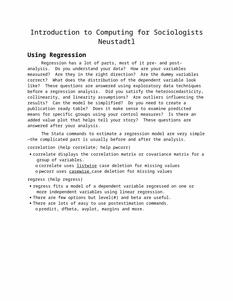
Introduction to Computing for SociologistsNeustadtl

Using RegressionRegression has a lot of parts, most of it pre- and post- analysis. Do you understand your data?

How are your variables measured? Are they in the right direction? Are the dummy variables correct? What does the distribution of the dependent variable look like? These questions are answered using ex-ploratory data techniques before a regression analysis. Did you satisfy the heteroscedasticity, collinearity, and linearity assumptions? Are outliers influencing the results? Can the model be simplified? Do you need to create a publication ready table? Does it make sense to examine predicted means for specific groups using your control measures? Is there an added value plot that helps tell your story? These ques-tions are answered after your analysis.

The Stata commands to estimate a regression model are very simple—the complicated part is usually before and after the analysis.

correlation (help correlate; help pwcorr) correlate displays the correlation matrix or covariance matrix for a group of variables.

o correlate uses listwise case deletion for missing valueso pwcorr uses casewise case deletion for missing values

regress (help regress) regress fits a model of a dependent variable regressed on one or more independent variables using

linear regression. There are few options but level(#) and beta are useful. There are lots of easy to use postestimation commands.

o predict, dfbeta, avplot, margins and more.

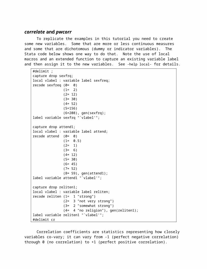
correlate and pwcorrTo replicate the examples in this tutorial you need to create some new variables. Some that are

more or less continuous measures and some that are dichotomous (dummy or indicator variables). The Stata code below shows one way to do that. Note the use of local macros and an extended function to capture an existing variable label and then assign it to the new variables. See -help local- for details.

#delimit ;capture drop sexfrq;local vlabel : variable label sexfreq;recode sexfreq (0= 0) (1= 2) (2= 12) (3= 30) (4= 52) (5=156) (6=208), gen(sexfrq);label variable sexfrq "`vlabel'";

capture drop attend1;local vlabel : variable label attend;recode attend (0= 0) (1= 0.5) (2= 1) (3= 6) (4= 12) (5= 30) (6= 45) (7= 52) (8= 59), gen(attend1);label variable attend1 "`vlabel'";

capture drop reliten1;local vlabel : variable label reliten;recode reliten (1= 1 "strong") (2= 3 "not very strong") (3= 2 "somewhat strong") (4= 4 "no religion"), gen(reliten1);label variable reliten1 "`vlabel'";#delimit cr

Correlation coefficients are statistics representing how closely variables co-vary; it can vary from -1 (perfect negative correlation) through 0 (no correlation) to +1 (perfect positive correlation). Typically correlations are a beginning point for examining linear relationships but, do not control for other variables like regression (though partial and semi-partial correlation both do). There are not many options but Stata has two distinct commands, correlate and pwcorr. Read the help file and look at the following exam-ples:

1. corr sexfrq age2. corr sexfrq age if year==20063. bysort year: corr sexfrq age

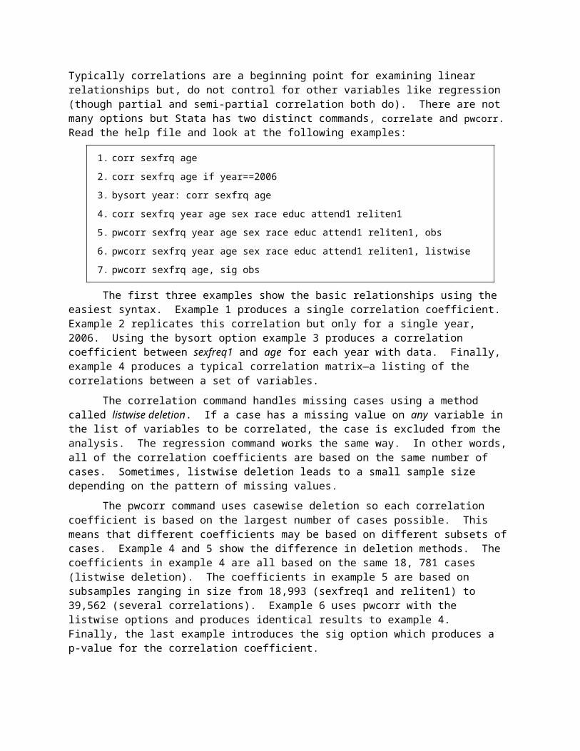
4. corr sexfrq year age sex race educ attend1 reliten15. pwcorr sexfrq year age sex race educ attend1 reliten1, obs6. pwcorr sexfrq year age sex race educ attend1 reliten1, listwise7. pwcorr sexfrq age, sig obs

The first three examples show the basic relationships using the easiest syntax. Example 1 pro-duces a single correlation coefficient. Example 2 replicates this correlation but only for a single year, 2006. Using the bysort option example 3 produces a correlation coefficient between sexfreq1 and age for each year with data. Finally, example 4 produces a typical correlation matrix—a listing of the correla-tions between a set of variables.

The correlation command handles missing cases using a method called listwise deletion. If a case has a missing value on any variable in the list of variables to be correlated, the case is excluded from the analysis. The regression command works the same way. In other words, all of the correlation coeffi-cients are based on the same number of cases. Sometimes, listwise deletion leads to a small sample size depending on the pattern of missing values.

The pwcorr command uses casewise deletion so each correlation coefficient is based on the largest number of cases possible. This means that different coefficients may be based on different subsets of cases. Example 4 and 5 show the difference in deletion methods. The coefficients in example 4 are all based on the same 18, 781 cases (listwise deletion). The coefficients in example 5 are based on subsam-ples ranging in size from 18,993 (sexfreq1 and reliten1) to 39,562 (several correlations). Example 6 uses pwcorr with the listwise options and produces identical results to example 4. Finally, the last example introduces the sig option which produces a p-value for the correlation coefficient.

1. Compare the correlation results for the variables sociability, sex, race, age, education, year attend1, and reliten1 using correlate and pwcorr. What is the strongest linear relationship?

2. The strongest relationship is between sociability and how often a person attends religious services. Is this relationship statistically significant for every year?

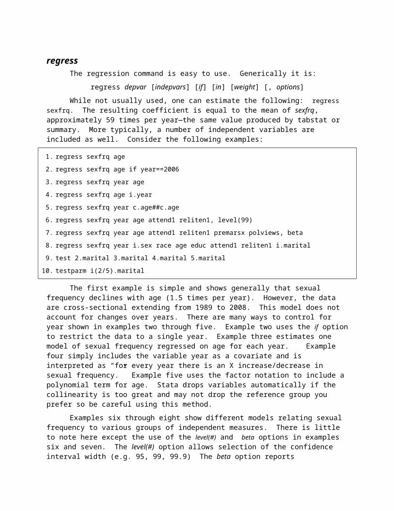
regressThe regression command is easy to use. Generically it is:

regress depvar [indepvars] [if] [in] [weight] [, options]While not usually used, one can estimate the following: regress sexfrq. The resulting coeffi-

cient is equal to the mean of sexfrq, approximately 59 times per year—the same value produced by tab-stat or summary. More typically, a number of independent variables are included as well. Consider the following examples:

1. regress sexfrq age2. regress sexfrq age if year==20063. regress sexfrq year age4. regress sexfrq age i.year5. regress sexfrq year c.age##c.age6. regress sexfrq year age attend1 reliten1, level(99)7. regress sexfrq year age attend1 reliten1 premarsx polviews, beta8. regress sexfrq year i.sex race age educ attend1 reliten1 i.marital9. test 2.marital 3.marital 4.marital 5.marital

10. testparm i(2/5).marital

The first example is simple and shows generally that sexual frequency declines with age (1.5 times per year). However, the data are cross-sectional extending from 1989 to 2008. This model does not account for changes over years. There are many ways to control for year shown in examples two through five. Example two uses the if option to restrict the data to a single year. Example three estimates one model of sexual frequency regressed on age for each year. Example four simply includes the variable year as a covariate and is interpreted as “for every year there is an X increase/decrease in sexual fre-quency.” Example five uses the factor notation to include a polynomial term for age. Stata drops vari-ables automatically if the collinearity is too great and may not drop the reference group you prefer so be careful using this method.

Examples six through eight show different models relating sexual frequency to various groups of independent measures. There is little to note here except the use of the level(#) and beta options in ex-amples six and seven. The level(#) option allows selection of the confidence interval width (e.g. 95, 99, 99.9) The beta option reports standardized coefficients instead of confidence intervals. The beta co-efficients are the regression coefficients obtained by first standardizing all variables to have a mean of 0 and a standard deviation of 1 (i.e. transformed to z-scores).

The last example, number eight, followed by hierarchical F-tests or change in R2 tests for groups of included variables. This is useful when your data story has a progressive logic. For example, if vari-ables can be categorized into groups like demographic (age, sex, and race), human capital (education, oc-cupational prestige, and years in the workforce), social capital (number of friends, sociability, etc.) and you want to compare the effect of these different blocks of measures.

Read the online help (help regress) and:

3. Regress sociability on year and age. Controlling for year, what is the relationship between age and sociability?

4. Suspecting a non-linear relationship between sociability and age, enter a quadratic term for age (i.e. age2) and control for year.

5. Regress sociability on year, sex, race, and education using the beta option to determine that vari-able that has the single greatest effect on sociability, controlling for the others.

6. Use the nestreg prefix to regress sociability on 1) year sex, race, age, and education; 2) marital dummy variables (drop married respondents); 3) religion measures (attend and reliten). You will need to create marital dummies (tabulate with the generate option is one easy method) and re-verse code the religion variables to associate larger values with greater religiosity.

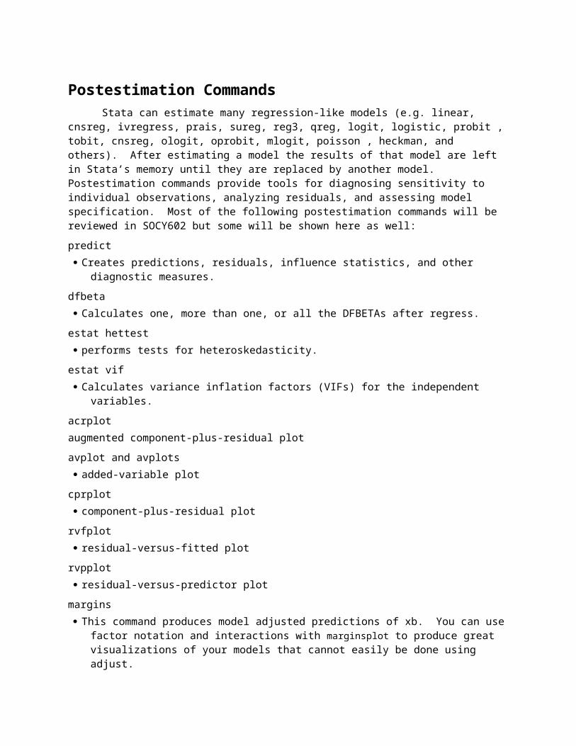
Postestimation CommandsStata can estimate many regression-like models (e.g. linear, cnsreg, ivregress, prais, sureg, reg3,

qreg, logit, logistic, probit , tobit, cnsreg, ologit, oprobit, mlogit, poisson , heckman, and others). After estimating a model the results of that model are left in Stata’s memory until they are replaced by another model. Postestimation commands provide tools for diagnosing sensitivity to individual observations, ana-lyzing residuals, and assessing model specification. Most of the following postestimation commands will be reviewed in SOCY602 but some will be shown here as well:

predict Creates predictions, residuals, influence statistics, and other diagnostic measures.

dfbeta Calculates one, more than one, or all the DFBETAs after regress.

estat hettest performs tests for heteroskedasticity.

estat vif Calculates variance inflation factors (VIFs) for the independent variables.

acrplotaugmented component-plus-residual plot

avplot and avplots added-variable plot

cprplot component-plus-residual plot

rvfplot residual-versus-fitted plot

rvpplot residual-versus-predictor plot

margins This command produces model adjusted predictions of xb. You can use factor notation and interac-

tions with marginsplot to produce great visualizations of your models that cannot easily be done using adjust.

Margins are statistics calculated from predictions of a previously fit model at fixed values of some covariates and averaging or otherwise integrating over the remaining covariates.

The margins command estimates margins of responses for specified values of covariates and presents the results as a table.

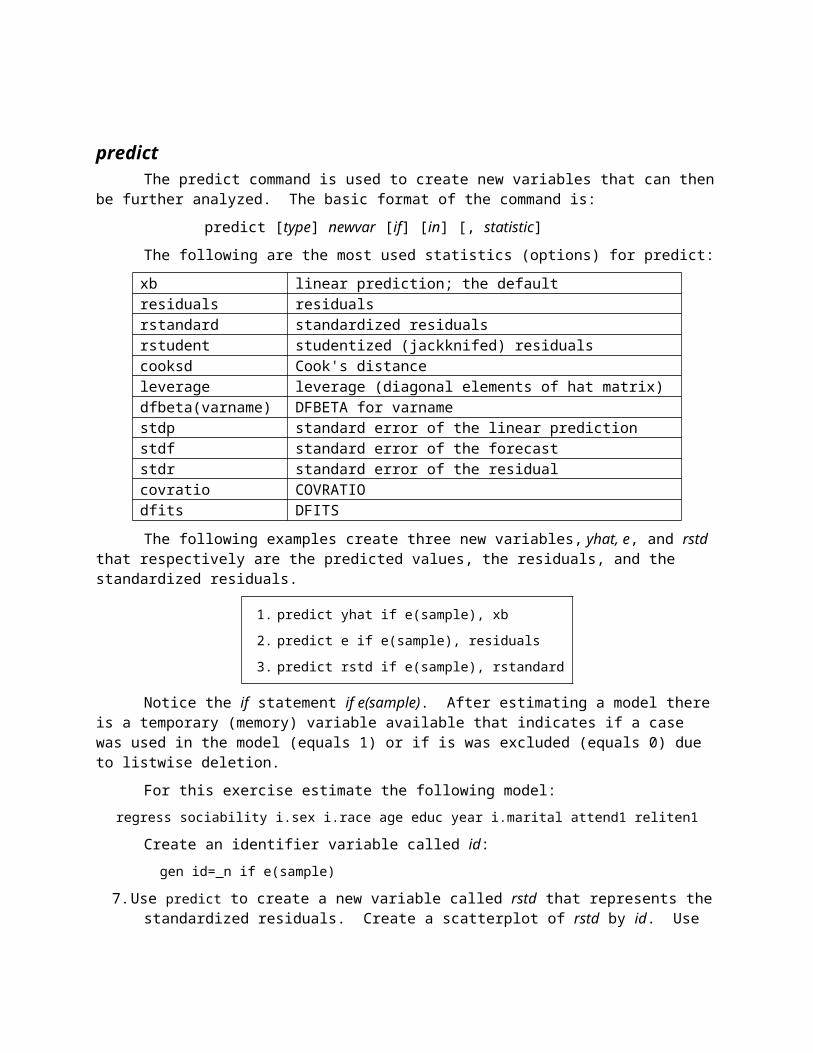
predictThe predict command is used to create new variables that can then be further analyzed. The ba-

sic format of the command is:

predict [type] newvar [if] [in] [, statistic]The following are the most used statistics (options) for predict:

xb linear prediction; the defaultresiduals residualsrstandard standardized residualsrstudent studentized (jackknifed) residualscooksd Cook's distanceleverage leverage (diagonal elements of hat matrix)dfbeta(varname) DFBETA for varnamestdp standard error of the linear predictionstdf standard error of the forecaststdr standard error of the residualcovratio COVRATIOdfits DFITSThe following examples create three new variables, yhat, e, and rstd that respectively are the pre-

dicted values, the residuals, and the standardized residuals.

1. predict yhat if e(sample), xb2. predict e if e(sample), residuals3. predict rstd if e(sample), rstandard

Notice the if statement if e(sample). After estimating a model there is a temporary (memory) variable available that indicates if a case was used in the model (equals 1) or if is was excluded (equals 0) due to listwise deletion.

For this exercise estimate the following model:

regress sociability i.sex i.race age educ year i.marital attend1 reliten1Create an identifier variable called id:

gen id=_n if e(sample)7. Use predict to create a new variable called rstd that represents the standardized residuals. Create a

scatterplot of rstd by id. Use the yline options to put thick, dashed lines at -1.96 and 1.96. Inter-pret this plot.

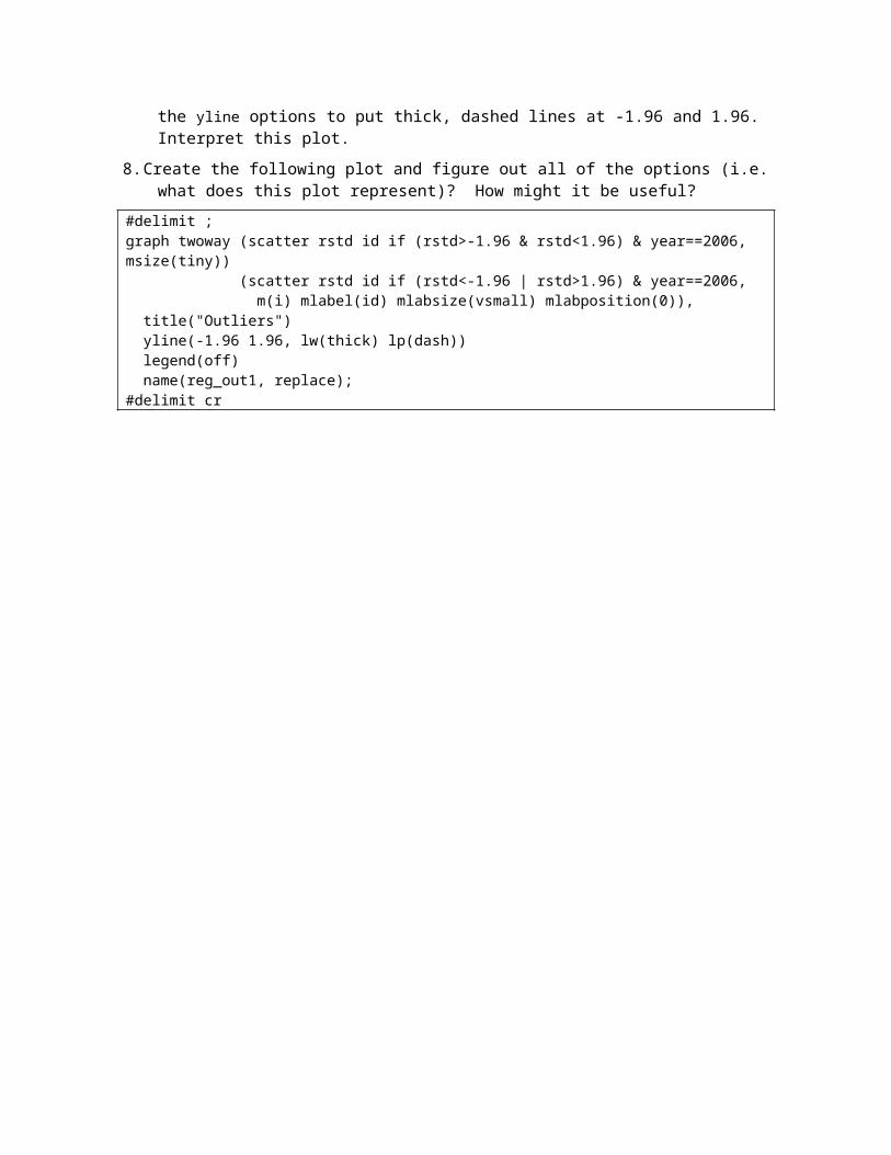
8. Create the following plot and figure out all of the options (i.e. what does this plot represent)? How might it be useful?

#delimit ;graph twoway (scatter rstd id if (rstd>-1.96 & rstd<1.96) & year==2006, msize(tiny)) (scatter rstd id if (rstd<-1.96 | rstd>1.96) & year==2006, m(i) mlabel(id) mlabsize(vsmall) mlabposition(0)), title("Outliers") yline(-1.96 1.96, lw(thick) lp(dash))

legend(off) name(reg_out1, replace);#delimit cr

estat hettest and estat vifThese two commands are used to test for heteroscedasticity and multicollinearity. These topics

will be covered in SOCY602 so no comments are offered here.

9. Produce the hettest (e.g. the Breusch-Pagan/Cook-Weisberg test) and the variance inflation factors (VIF’s).

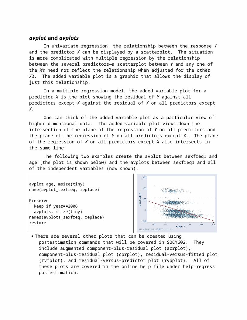
avplot and avplotsIn univariate regression, the relationship between the response Y and the predictor X can be dis-

played by a scatterplot. The situation is more complicated with multiple regression by the relationship between the several predictors—a scatterplot between Y and any one of the X’s need not reflect the rela-tionship when adjusted for the other X’s. The added variable plot is a graphic that allows the display of just this relationship.

In a multiple regression model, the added variable plot for a predictor X is the plot showing the residual of Y against all predictors except X against the residual of X on all predictors except X.

One can think of the added variable plot as a particular view of higher dimensional data. The added variable plot views down the intersection of the plane of the regression of Y on all predictors and the plane of the regression of Y on all predictors except X. The plane of the regression of X on all predic-tors except X also intersects in the same line.

The following two examples create the avplot between sexfreq1 and age (the plot is shown be-low) and the avplots between sexfreq1 and all of the independent variables (now shown).

avplot age, msize(tiny) name(avplot_sexfreq, re-place)

Preserve keep if year==2006 avplots, msize(tiny) names(avplots_sexfreq, re-place)restore

There are several other plots that can be created using postestimation commands that will be covered in SOCY602. They include augmented component-plus-residual plot (acrplot), component-plus-residual plot (cprplot), residual-versus-fitted plot (rvfplot), and residual-versus-predictor plot (rvpplot). All of these plots are covered in the online help file under help regress postesti-mation.

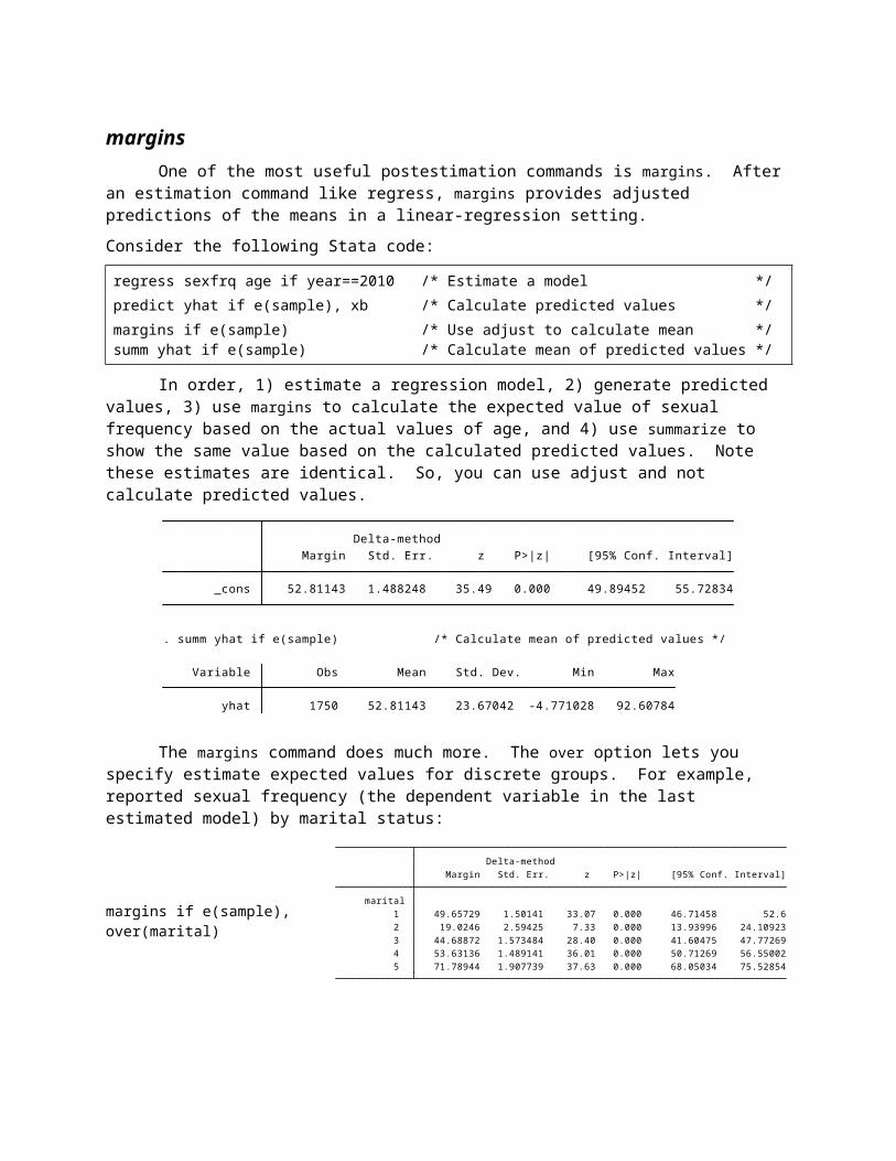
marginsOne of the most useful postestimation commands is margins. After an estimation command like

regress, margins provides adjusted predictions of the means in a linear-regression setting.

Consider the following Stata code:

regress sexfrq age if year==2010 /* Estimate a model */predict yhat if e(sample), xb /* Calculate predicted values */margins if e(sample) /* Use adjust to calculate mean */summ yhat if e(sample) /* Calculate mean of predicted values */

In order, 1) estimate a regression model, 2) generate predicted values, 3) use margins to calcu-late the expected value of sexual frequency based on the actual values of age, and 4) use summarize to show the same value based on the calculated predicted values. Note these estimates are identical. So, you can use adjust and not calculate predicted values.

The margins command does much more. The over option lets you specify estimate expected values for discrete groups. For example, reported sexual frequency (the dependent variable in the last es-timated model) by marital status:

margins if e(sample), over(marital)

yhat 1750 52.81143 23.67042 -4.771028 92.60784 Variable Obs Mean Std. Dev. Min Max

. summ yhat if e(sample) /* Calculate mean of predicted values */

_cons 52.81143 1.488248 35.49 0.000 49.89452 55.72834 Margin Std. Err. z P>|z| [95% Conf. Interval] Delta-method

5 71.78944 1.907739 37.63 0.000 68.05034 75.52854 4 53.63136 1.489141 36.01 0.000 50.71269 56.55002 3 44.68872 1.573484 28.40 0.000 41.60475 47.77269 2 19.0246 2.59425 7.33 0.000 13.93996 24.10923 1 49.65729 1.50141 33.07 0.000 46.71458 52.6 marital Margin Std. Err. z P>|z| [95% Conf. Interval] Delta-method

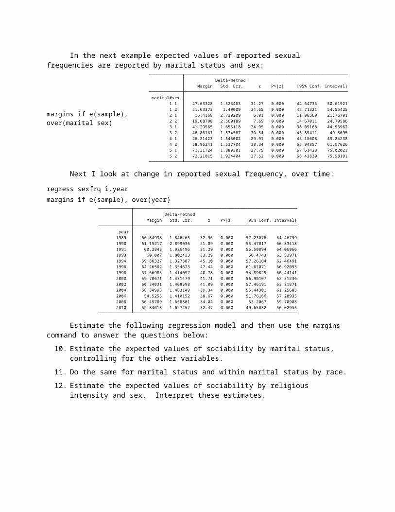
In the next example expected values of reported sexual frequencies are reported by marital status and sex:

margins if e(sample), over(marital sex)

Next I look at change in reported sexual frequency, over time:

regress sexfrq i.yearmargins if e(sample), over(year)

Estimate the following regression model and then use the margins command to answer the ques-tions below:

10. Estimate the expected values of sociability by marital status, controlling for the other variables.

11. Do the same for marital status and within marital status by race.

12. Estimate the expected values of sociability by religious intensity and sex. Interpret these estimates.

5 2 72.21015 1.924404 37.52 0.000 68.43839 75.98191 5 1 71.31724 1.889301 37.75 0.000 67.61428 75.02021 4 2 58.96241 1.537704 38.34 0.000 55.94857 61.97626 4 1 46.21423 1.545002 29.91 0.000 43.18608 49.24238 3 2 46.86181 1.534567 30.54 0.000 43.85411 49.8695 3 1 41.29565 1.655118 24.95 0.000 38.05168 44.53962 2 2 19.68798 2.560189 7.69 0.000 14.67011 24.70586 2 1 16.4168 2.730209 6.01 0.000 11.06569 21.76791 1 2 51.63373 1.49009 34.65 0.000 48.71321 54.55425 1 1 47.63328 1.523463 31.27 0.000 44.64735 50.61921 marital#sex Margin Std. Err. z P>|z| [95% Conf. Interval] Delta-method

2010 52.84018 1.627257 32.47 0.000 49.65082 56.02955 2008 56.45789 1.658801 34.04 0.000 53.2067 59.70908 2006 54.5255 1.410152 38.67 0.000 51.76166 57.28935 2004 58.34993 1.483149 39.34 0.000 55.44301 61.25685 2002 60.34031 1.468598 41.09 0.000 57.46191 63.21871 2000 59.70671 1.431479 41.71 0.000 56.90107 62.51236 1998 57.66983 1.414097 40.78 0.000 54.89825 60.44141 1996 64.26582 1.354673 47.44 0.000 61.61071 66.92093 1994 59.86327 1.327387 45.10 0.000 57.26164 62.46491 1993 60.007 1.802433 33.29 0.000 56.4743 63.53971 1991 60.2848 1.926496 31.29 0.000 56.50894 64.06066 1990 61.15217 2.899036 21.09 0.000 55.47017 66.83418 1989 60.84938 1.846265 32.96 0.000 57.23076 64.46799 year Margin Std. Err. z P>|z| [95% Conf. Interval] Delta-method

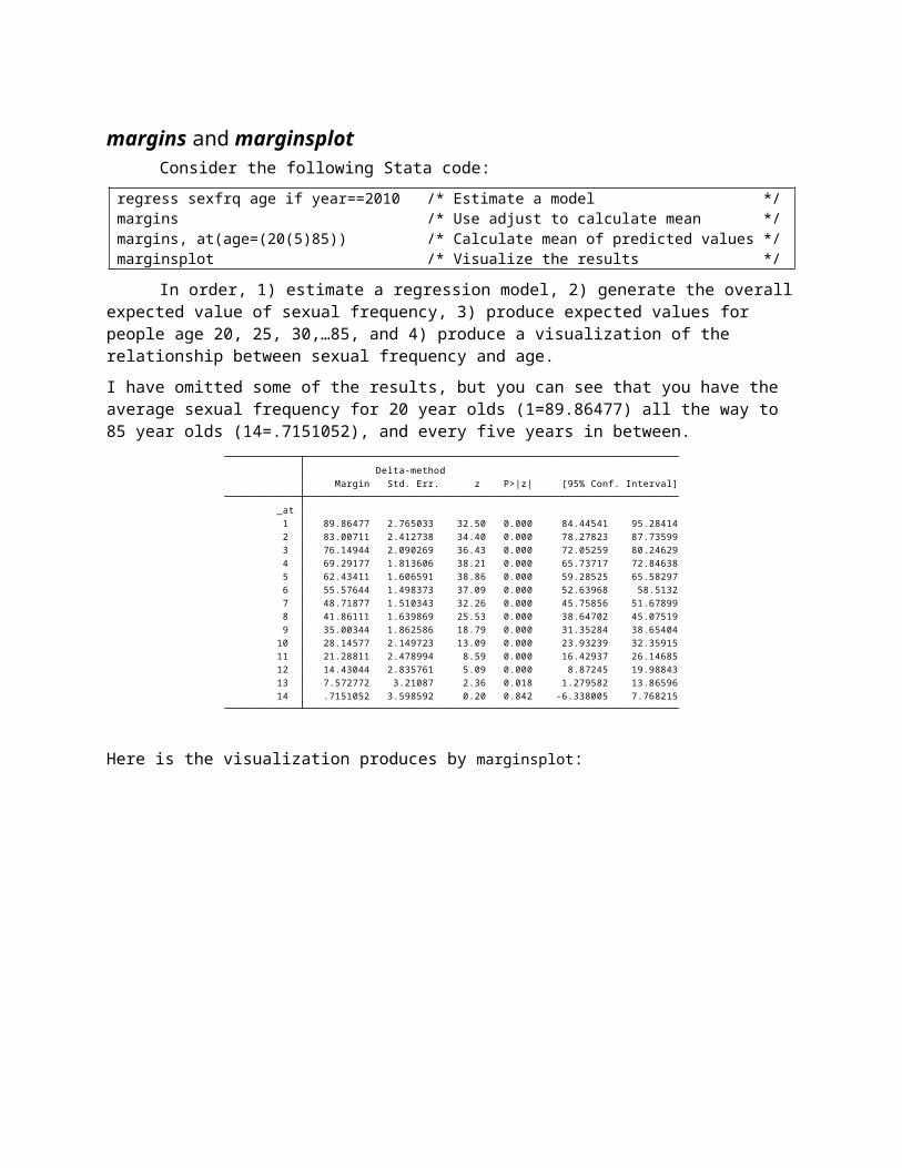
margins and marginsplotConsider the following Stata code:

regress sexfrq age if year==2010 /* Estimate a model */margins /* Use adjust to calculate mean */margins, at(age=(20(5)85)) /* Calculate mean of predicted values */marginsplot /* Visualize the results */

In order, 1) estimate a regression model, 2) generate the overall expected value of sexual fre-quency, 3) produce expected values for people age 20, 25, 30,…85, and 4) produce a visualization of the relationship between sexual frequency and age.

I have omitted some of the results, but you can see that you have the average sexual frequency for 20 year olds (1=89.86477) all the way to 85 year olds (14=.7151052), and every five years in between.

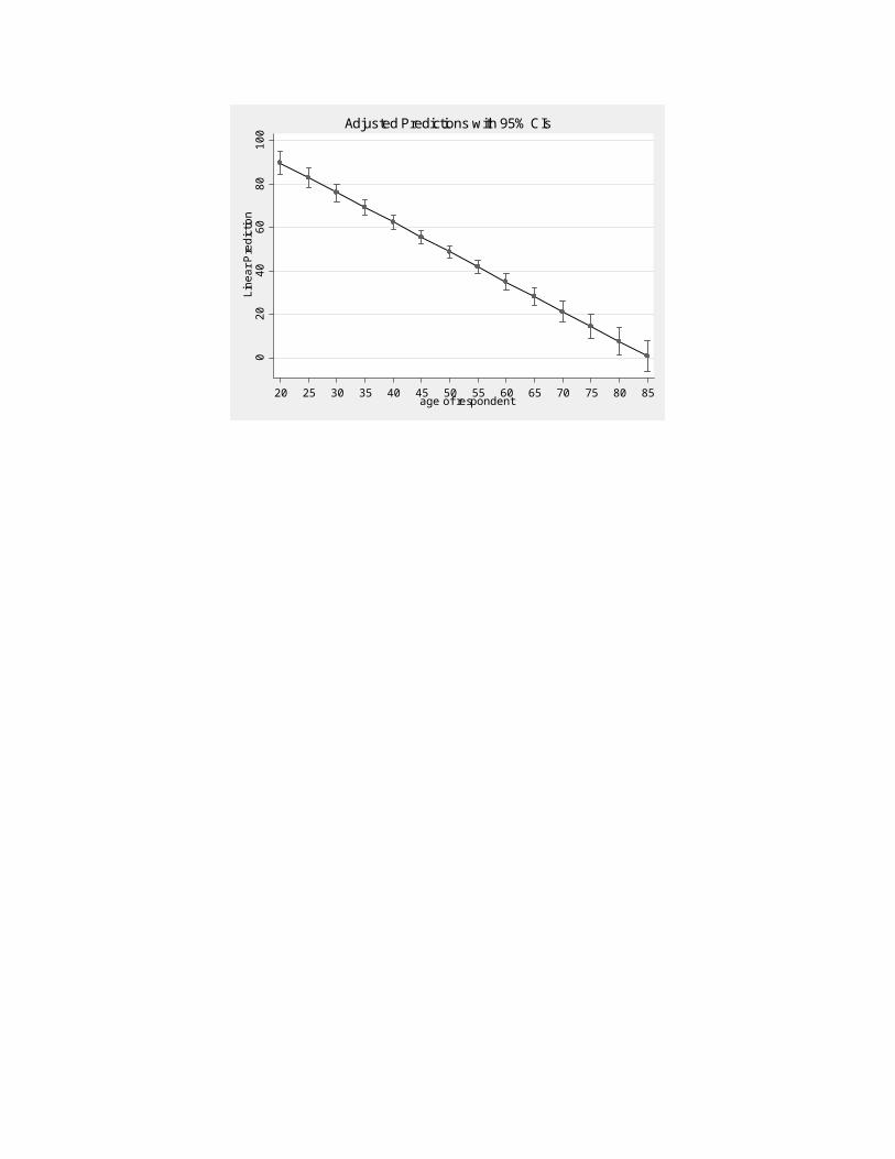
Here is the visualization produces by marginsplot:

14 .7151052 3.598592 0.20 0.842 -6.338005 7.768215 13 7.572772 3.21087 2.36 0.018 1.279582 13.86596 12 14.43044 2.835761 5.09 0.000 8.87245 19.98843 11 21.28811 2.478994 8.59 0.000 16.42937 26.14685 10 28.14577 2.149723 13.09 0.000 23.93239 32.35915 9 35.00344 1.862586 18.79 0.000 31.35284 38.65404 8 41.86111 1.639869 25.53 0.000 38.64702 45.07519 7 48.71877 1.510343 32.26 0.000 45.75856 51.67899 6 55.57644 1.498373 37.09 0.000 52.63968 58.5132 5 62.43411 1.606591 38.86 0.000 59.28525 65.58297 4 69.29177 1.813606 38.21 0.000 65.73717 72.84638 3 76.14944 2.090269 36.43 0.000 72.05259 80.24629 2 83.00711 2.412738 34.40 0.000 78.27823 87.73599 1 89.86477 2.765033 32.50 0.000 84.44541 95.28414 _at Margin Std. Err. z P>|z| [95% Conf. Interval] Delta-method

020

4060

8010

0Li

near

Pre

dict

ion

20 25 30 35 40 45 50 55 60 65 70 75 80 85age of respondent

Adjusted Predictions with 95% CIs

Installing Useful User-Written Stata Programs

User-written programsStata has a somewhat open architecture that allows users to write their own Stata programs for

tasks that they perform repetitively. There are lots of user-written commands for use with Stata. With Stata’s Internet features, obtaining these programs is relatively easy.

Two programs that you might find particularly useful are vreverse and estout.

vreverse generates newvar as a reversed copy of an existing categorical variable varname which has integer values and (usually) value labels assigned. Suppose that in the observations specified varname varies between minimum min and maxi-mum max. Then newvar = min + max – varname and any value labels are mapped accordingly. If no value labels have been assigned, then the values of varname will become the value labels of newvar. newvar will have the same storage type and the same display format as varname. If varname possesses a variable label or charac-teristics, these will also be copied. It is the user's responsibility to consider whether the copied variable label and characteristics also apply to newvar.

estout produces a table of regression results from one or several models for use with spreadsheets, LaTeX, HTML, or a word-processor table. eststo stores a quick copy of the active estimation results for later tabulation. esttab is a wrap-per for estout. It displays a pretty looking publication-style regression table with-out much typing. estadd adds additional results to the e()-returns for one or sev-eral models previously fitted and stored. This package subsumes the previously cir-culated esto, esta, estadd, and estadd_plus. An earlier version of estout is available as estout1.

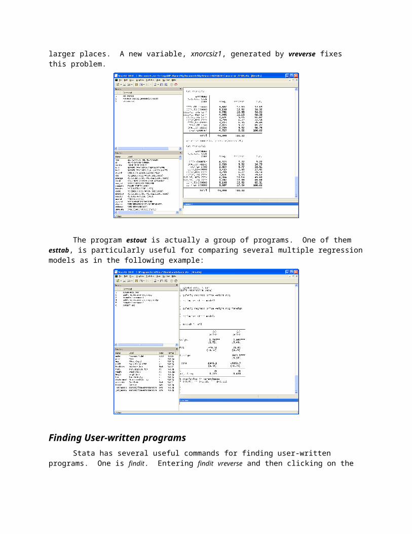
For example, vreverse reorders values and value labels of a variable. In the following screen capture see how the xnorsiz measure is in the wrong direction—smaller numerical values are associated with larger places. A new variable, xnorcsiz1, generated by vreverse fixes this problem.

The program estout is actually a group of programs. One of them esttab, is particularly use-ful for comparing several multiple regression models as in the following example:

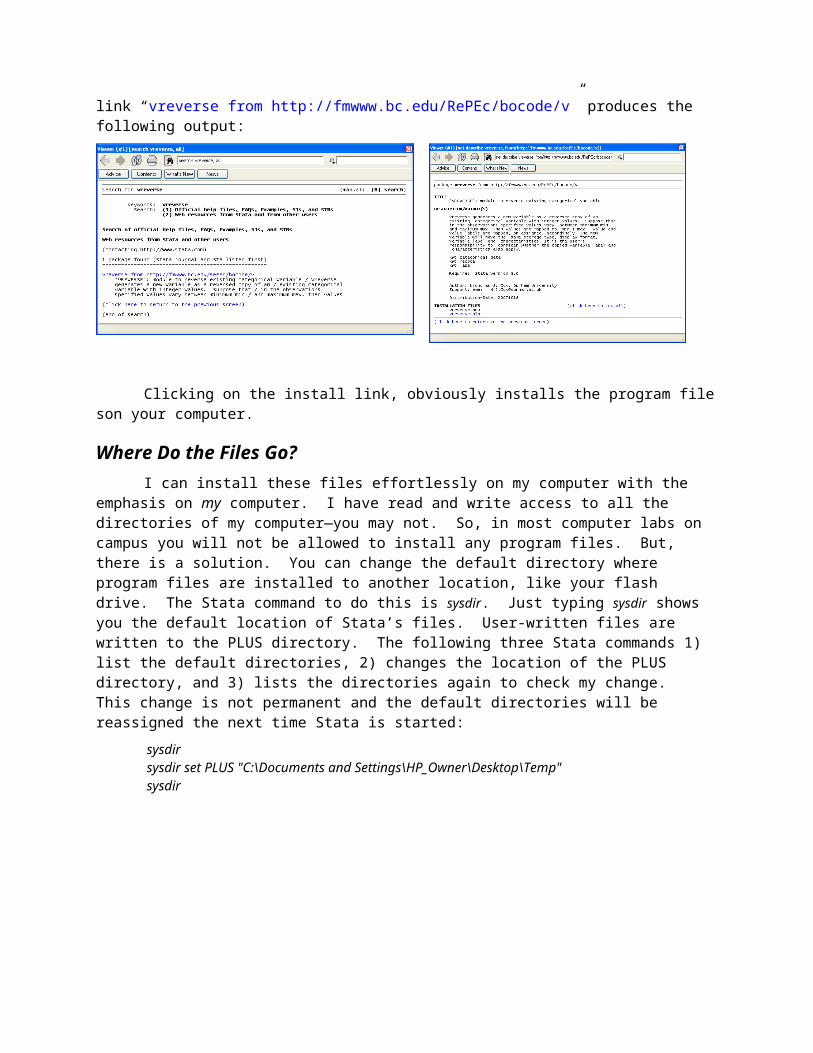
Finding User-written programsStata has several useful commands for finding user-written programs. One is findit. Entering

findit vreverse and then clicking on the link “vreverse from http://fmwww.bc.edu/RePEc/bocode/v” produces the following output:

Clicking on the install link, obviously installs the program file son your computer.

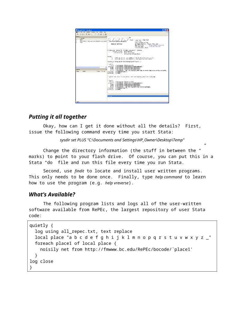
Where Do the Files Go?I can install these files effortlessly on my computer with the emphasis on my computer. I have

read and write access to all the directories of my computer—you may not. So, in most computer labs on campus you will not be allowed to install any program files. But, there is a solution. You can change the default directory where program files are installed to another location, like your flash drive. The Stata command to do this is sysdir. Just typing sysdir shows you the default location of Stata’s files. User-written files are written to the PLUS directory. The following three Stata commands 1) list the default di-

rectories, 2) changes the location of the PLUS directory, and 3) lists the directories again to check my change. This change is not permanent and the default directories will be reassigned the next time Stata is started:

sysdirsysdir set PLUS "C:\Documents and Settings\HP_Owner\Desktop\Temp"sysdir

Putting it all togetherOkay, how can I get it done without all the details? First, issue the following command every

time you start Stata:

sysdir set PLUS "C:\Documents and Settings\HP_Owner\Desktop\Temp"

Change the directory information (the stuff in between the “” marks) to point to your flash drive. Of course, you can put this in a Stata “do” file and run this file every time you run Stata.

Second, use findit to locate and install user written programs. This only needs to be done once. Finally, type help command to learn how to use the program (e.g. help vreverse).

What’s Available?The following program lists and logs all of the user-written software available from RePEc, the

largest repository of user Stata code:

quietly { log using all_repec.txt, text replace local place "a b c d e f g h i j k l m n o p q r s t u v w x y z _" foreach place1 of local place { noisily net from http://fmwww.bc.edu/RePEc/bocode/`place1' }log close}

Outputting Regression Results

Esttab and estoutStata produces output in the results window. For publication quality tables many people organize

this output in a table in MS Word or MS Excel and type the results into the table. This is time consuming and often leads to data entry errors.

The command estout is a command, actually a set of commands, written by Ben Jann to create publication quality tables in the results window or written to a file that can be imported to other software applications (e.g. Word and Excel). Because it is a user-written command you must install the program before you can use it. The program assembles a table of coefficients, “significance stars”, summary sta-tistics, standard errors, t- or z-statistics, p-values, confidence intervals, and other statistics for one or more models previously fitted and stored by estimates store or eststo. It then displays the table in Stata’s results window or writes it to a text file specified by using. The default is to use SMCL formatting tags and horizontal lines to structure the table. However, if using is specified, a tab-delimited table without lines is produced. This file can easily be imported to MS Word or MS Excel. Lots of detailed informa-tion is available at repec.org/bocode/e/estout/index.html.

The three most important commands are eststo (stores model estimates), esttab (displays for-matted regression results in the results window), and estout (writes regression results to a file for use in other programs).

esttab—screen displayConsider the following example and screen capture from the results window:

quietly eststo: regress sexfrq year c.age##c.agequietly eststo: regress sexfrq year c.age##c.age i.sex i.race educ childsesttabeststo clear

The prefix estto stores the last estimation results so they can be reformatted by esttab (or estout). The quietly command is used to suppress the normal Stata regression output. Here, esttab is used with no options and the output looks pretty good. Finally, eststo clear is used to remove the stored results.

* p<0.05, ** p<0.01, *** p<0.001t statistics in parentheses N 24326 24233 (4.08) (3.35) _cons 531.5*** 436.4***

(16.82) childs 4.673***

(-1.54) educ -0.224

(-2.71) 3.race -4.591**

(0.41) 2.race 0.506

(.) 1b.race 0

(-11.14) 2.sex -9.065***

(.) 1b.sex 0

(-6.60) (-3.31) c.age#c.age -0.00860*** -0.00445***

(-5.10) (-9.25) age -0.670*** -1.271***

(-3.24) (-2.37) year -0.211** -0.155* sexfrq sexfrq (1) (2)

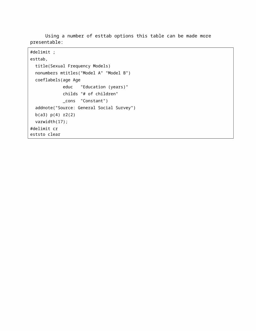
Using a number of esttab options this table can be made more presentable:

#delimit ;esttab, title(Sexual Frequency Models) nonumbers mtitles("Model A" "Model B") coeflabels(age Age educ "Education (years)" childs "# of children" _cons "Constant") addnote("Source: General Social Survey") b(a3) p(4) r2(2) varwidth(17);#delimit creststo clear

estoutThe estout assembles a regression table from one or more models previously fitted and stored

and writes it to a file so it can be imported to other software applications like MS Word and MS Excel. The full syntax of estout is rather complex and is to be found in the help file. In some sense there is lit-tle difference between estout and esttab, but estout seems to have more options for fine tuning a qual-ity table. The esttab command is easier to use but not as good for publication quality tables.

Consider the following estout commands and output:

quietly eststo: regress sexfrq year c.age##c.agequietly eststo: regress sexfrq year c.age##c.age i.sex i.race educ childs#delimit ;estout, title(Table 1. Sexual Frequency Models) mlabels("Baseline" "Full")

* p<0.05, ** p<0.01, *** p<0.001Source: General Social Surveyp-values in parentheses R-sq 0.16 N 24233 (0.0008) Constant 436.4***

(0.0000) # of children 4.673***

(0.1243) Education (years) -0.224

(0.0067) 3.race -4.591**

(0.6813) 2.race 0.506

(.) 1b.race 0

(0.0000) 2.sex -9.065***

(.) 1b.sex 0

(0.0009) c.age#c.age -0.00445***

(0.0000) Age -1.271***

(0.0176) year -0.155* Model A Sexual Frequency Models

note("Source: General Social Survey, 1972-2006") cells(b(star fmt(%8.4f) label(Coef)) se(par fmt(%8.4f))) stats(r2 N, fmt(3 %7.0fc) labels(R-squared "N of cases")) label legend varlabels(_cons Constant year "Survey Year" age Age agesqr Age-squared sex "Sex (0=M/1=F)" race "Race (0=W/1=B)" educ "Years of Education" childs "# of children");#delimit cr

A lot of options were used here to create a reasonably good looking table comparing these two models. For example, titles and labels were created for the table, the models, and a note about the source of the data. Further, the cells content was determined and formatted (coefficients with significance stars and standard errors—se in parentheses, etc.) and the independent variables were relabeled. Finally, a leg-end indicating the significance levels was added.

Once a reasonably good looking table is produces it can be written in a tab-delimited file format to a file. Tab-delimited information is something of a lingua franca for Windows based software applica-tions. Creating this file is easy. The command to write the table to a file is:

estout using example.txt, replace

* p<0.05, ** p<0.01, *** p<0.001Source: General Social Survey, 1972-2006 N of cases 24,233 R-squared 0.160 (130.3198) Constant 436.4408*** (0.2778) # of children 4.6727*** (0.1459) Years of Education -0.2243 (1.6941) 3.race of respondent -4.5909** (1.2314) 2.race of respondent 0.5057 (.) 1b.race of respond~t 0.0000 (0.8139) 2.respondents sex -9.0653*** (.) 1b.respondents sex 0.0000 (0.0013) c.age#c.age -0.0044*** (0.1375) Age -1.2714*** (0.0653) Survey Year -0.1550* Coef/se Baseline Table 1. Sexual Frequency Models

quietly eststo: regress sexfreq1 year age agesqrquietly eststo: regress sexfreq1 year age agesqr sex race educ childs#delimit ;estout using example.txt, replace title(Table 1. Sexual Frequency Models) mlabels("Baseline" "Full") note("Source: General Social Survey, 1972-2006") cells(b(star fmt(%8.4f) label(Coef)) se(par fmt(%8.4f))) stats(r2 N, fmt(3 %7.0fc) labels(R-squared "N of cases")) label legend varlabels(_cons Constant year "Survey Year" age Age agesqr Age-squared sex "Sex (0=M/1=F)" race "Race (0=W/1=B)" educ "Years of Education" childs "# of children");#delimit cr

After copying-and-pasting the content of example.txt into MS Word and some editing the final ta-ble is:

Table 1. Sexual Frequency ModelsBaseline FullCoef/se Coef/se

Survey Year -0.2112** -0.1550*(0.0652) (0.0653)

Age -0.6700*** -1.2714***(0.1313) (0.1375)

c.age#c.age -0.0086*** -0.0044***(0.0013) (0.0013)

2.respondents sex -9.0653***(0.8139)

2.race of respondent 0.5057(1.2314)

3.race of respondent -4.5909**(1.6941)

Years of Education -0.2243(0.1459)

# of children 4.6727***(0.2778)

Constant 531.4707*** 436.4408***(130.3070) (130.3198)

R-squared 0.146 0.160N of cases 24,326 24,233Source: General Social Survey, 1972-2006* p<0.05, ** p<0.01, *** p<0.001

Warning! This can take a lot of time until you learn how to use all of the options in estout and table sin MS Word. If we have time we can review editing tables in MS Word. You only want to invest your time in making pretty tables when you are pretty certain you have the results you want to present. Otherwise, simply use esttab to view the results in the results window as you experiment with different models.

13. Use eststo and esttab to 1) store the estimates from three regression models, and 2) display them efficiently in the results window. The baseline model or first model is sociability regressed on sex, race, age, educ, and year. For the second model add the marital status dummies to this model excluding the married dummy (w, d, s, and nm). Finally, add the religion variables (at-tend1 and reliten1) to this model.

14. Use estout to display the same information.

15. Use estout to produce a clean looking table (titles, source, variable labels, etc.)

16. Write this table to a file in tab-delimited format.

xml_tabAnother user-written alternative to estout is xml_tab. The program xml_tab saves Stata output

directly into XML file that could be opened with Microsoft Excel. The program is relatively flexible and produces print-ready tables in Excel and allows users to apply different formats to the elements of the out-put table and essentially do everything MS Excel can do in terms of formatting from within Stata.

The following is a simple example:

/* estout problems */quietly regress sociability year i.sex i.race age educestimates store m1quietly regress sociability year i.sex i.race age educ i.maritalestimates store m2quietly regress sociability year i.sex i.race age educ i.marital attend1 reliten1estimates store m3xml_tab m1 m2 m3, replaceestimates clear

The logic is similar to estout—regression models are estimated and the results are stored. Then these results are output in an MS Excel format. Stata has a command to store estimates. For example: estimates store m1. This creates a file called “stata_out.xml”. Double clicking on the file opens the file in MS Excel on most Windows based computers