Preliminary and incomplete Please do not quote

Do purified technological shocks support the RBC model?

–Empirical evidence from Japanese industry data-

August, 2005

Tsutomu Miyagawa (Gakushuin University) Yukie Sakuragawa (Atomi University)

Miho Takizawa (Hitotsubashi University)

1. Introduction

Since a seminal paper by Hayashi and Prescott (2002) published, a number of Japanese economists have focused on that technological progress which is represented by growth in Solow residual or total factor productivity affected the long-term stagnation of the Japanese economy. Following Hall (1988), (1990) and Basu and Fernald (1995), (1997), Kawamoto (2004) and Miyagawa, Sakuragawa, and Takizawa (2005) (hereafter MST) examined factors of Solow residual in Japan by estimating production functions by industry. While Kawamoto (2004) emphasized that utilization rates of labor and capital played a crucial role in the fluctuations in Solow residual, MST (2005) concluded that a purified technological shock which excluded the effect of increasing return to scale, utilization rate, and demand externalities from the traditional Solow residual was a key factor of the traditional Solow residual. Using micro-firm data, Nishimura, Nakajima and Kiyota (2005) and Fukao and Kwon (2005) showed that remaining low productivity firms reduced aggregate total factor productivity. Caballero, Hoshi and Kashyap (2004) checked whether low productivity firms were supported by financial intermediations.

However, the above results do not necessarily show the plausibility of RBC model in the short run. Presenting a new Keynesian dynamic general equilibrium model, Gali (1999) showed that technological shocks reduced labor hours in the short run in contrast with RBC model. His empirical works supported new Keynesian sticky price model in most of the advanced countries. Being inspired by Gali’s paper, a number of economists have studied the responses of macroeconomic variables such as labor hours, output, and investment to technological shocks in order to check the plausibility of RBC model in the short run.

While Gali (1999) estimated a structural VAR model to check the effects of technological shocks, Basu, Fernald and Kimball (2004) (hereafter, BFK) picked up pure technological shock by assuming that firms optimized cost function under imperfect competition. They estimated production function considering utilization rates of labor and capital by industry and aggregated pure technological shocks in each industry. They showed that the aggregate technological shocks reduced labor hours as Gali (1999) showed.

Following BFK (2004), two papers attacked this issue by using industry-level or micro-firm data. Malley, Muscatteli, and Woitek(2005) (hereafter MMW) proposed another macro model with sticky wages in addition to the standard RBC model and the sticky price model. In their sticky wage model, the movement of real wages is

1

ambiguous because technological shocks increases labor demand and causes price to fall, while real wages decrease by technological shock in the sticky price model. They measured not only Solow residual but also purified technological shock (modified Solow residual) by industry. They estimated VAR model at the industry level, including three endogenous variables: output, effective labor (or employment) and real wages. Their estimating results supported the RBC model or the sticky wage model. Marchetti and Nucci (2005) examined effects of technological shocks on labor hours by using micro-firm data (manufacturing sector). They also used BFK’s cost function, considering adjustment cost function and the effect of utilization on capital depreciation. Estimating production functions of the panel data, they picked up purified technological shock in each firm. By regressing labor index on a purified technological shock in each firm, they showed that technological shock reduced labor inputs. However, as Gali (1999) and BFK (2004) showed, the negative effect of technological shock on labor inputs is observed in the case of the labor reallocation model as well as the sticky price model. Then, they showed that technological shocks in firms with stickier price had contractionary effect on labor inputs.

In Japan, Braun and Shioji (2004) examined the responses of work hours to technological shocks. Following Gali (1999) and Uhlig (2001), they estimated VAR model with long-run restriction, sign restriction, and range restriction. Their estimation results supported a positive response of work hours to a positive technological shock, though the standard structural VAR model supported Gali’s results. In contrast with the results by Braun and Shioji (2004), Kawamoto and Nakakuki (2005) showed the contractionary effects of a positive technological shock. Following BFK (2004), they used industry-based data (KEO database) and picked up aggregate purified technological shocks by estimating production functions by industry. By estimating bivariate VAR model with aggregate purified technological shocks, they found that not only labor inputs but also investment responded negatively to a positive technological shock.

The above studies not only check the plausibility of several macro models but also help to understand the effectiveness of economic policies. If Gali’s result is plausible, Keynesian type macro economic policies are effective in the short run. However, if RBC model is supported, structural reform policies such as policies promoting R&D should be carried out.

Following the above studies, we check responses of aggregate variables to a positive technological shock by using industry-based data and measuring purified technological shocks. Though our study in the paper is similar to Kawamoto and Nakakuki (2005), our data using Financial Statements Statistics of Corporations

2

(hereafter FSSC) published Ministry of Finance covers not only the manufacturing sector but also non-manufacturing sector, while Kawamoto and Nakakuki (2005)’s paper focused on the manufacturing sector.

BFK (2004) and Marchetti and Nucci (2005) provided alternative models to the standard RBC model, when a negative response of labor hours to a positive technological shock was found. In contrast with Kawamoto and Nakakuki (2005)’s paper, we check the plausibility of alternative macro models after we find a negative response of labor hours.

The outline of our paper is as follows. In the next section, explaining cost minimizing model in BFK (2004), we estimate production function by industry. As MST (2005), we use FSSC quarterly data. In the third section, checking some features of Solow residual and aggregate pure technological shock, we examine the effect of aggregate pure technological shock on macroeconomic variables. In the last section, we summarize our results and state the future research agenda. 2. Measuring purified technological shock In this section, following BFK(2004), we measure a purified technological shock by

industry. Gross output in industry is described as i

(1) , ),,,( ititititit MZLFY Θ=

where denotes gross output, the effective labor input, the effective capital service, stands for intermediate inputs of energy and materials, and is defined as purified technological index. Here,

itY itL itZ

itM itΘ

itL )( ititit EHN= is decomposed into three factors; the number of employees , labor hours per workers , and labor effort

and consists of capital stock ( ) and capital utilization rate ( ), such that . The function is assumed to be homogenous of degree

itN itH

itE itZ itK itU

ititit UKZ = )(⋅F γ in total inputs. We observe only the number of employees ( ), labor hours per workers ( ), capital stock ( ), and intermediate inputs ( ). Labor effort ( ) and capital utilization rate ( ) are not observed.

itN itH

itK itM itE

itU Taking log of all variables in equation (1), differentiating them with respect to time, and separating the observed inputs and the unobserved inputs leads to

)2( itititiit hxy θγ ∆+∆+∆=∆ )( ,

where

itMiitZiititLiit mckchncx ∆+∆+∆+∆≡∆ )(

itZiitLiit uceca ∆+∆≡∆ .

3

For any variable , represents the growth rate of and denotes

cost-based share of factor .

itQ itq∆ itQ jic

jFollowing BFK(2002), we assume that firms face adjustment costs to investment and

hiring. Moreover, we assume that higher utilization or higher effort must raise firms cost, and longer labor hours also raise firms cost because of premium shift to compensate employees for working at night or other undesirable time. Firms minimize the present value of expected cost subject to equation (1), capital accumulation and labor hiring.

∑ ∏∞

− =

− Λ+Ψ+++ts

IM

s

ttOJMUEH K

JKPNOWNMPUXEHWNGrEMin )]()()(),(][)1([)3( 1

,,,,, ττ ,

subject to ititti KJK )1(1 δ−+=+ ,

and , ititti NON +=+1

where is discount rate of the firm, is a base wage, is a price of intermediate inputs, is a price of investment goods,O is labor hiring net of separations and is gross investment. The functions

tr W MP

IP J)(⋅Ψ and )(⋅Λ are adjustment cost functions of labor

hiring and investment, respectively. The function specifies how the hourly

wage depends on the length of the workday and effort and is shift premium.

Thus, represents the total compensation associated with

movements of labor hours, labor efforts, and capital utilization,

),( EHG

)(UX

)(),( UXEHWNG

)( NOWNΨ represents

the total cost of changing the number of employees, and )( KJKPI Λ represents the

total cost of investment. δ is the depreciation rate. Following the first order conditions, we obtain an equation implicitly relating E and H :

),(),(

),(),(

EHGEHEG

EHGEHHG EH = ,

where ( ) denotes the derivative of the labor cost function with respect to .

The elasticity of labor cost with respect to sG EHs ,= s

E and H must be equal because elasticity of effective labor input with respect E and H are equal in terms of benefits. From this relation and the assumption of , we can express unobserved intensity of labor utilization

GE as a function of observed hours per worker H , i.e. , )(HEE =

4

0)(' >HE . We define ξ as the elasticity of effort with respect to hours, we find the relation that dhde ξ= .

Following the first order conditions, we obtain an equation implicitly relating and UH :

])()('[]

),(),([

// 1

UXUUX

EHGEHHG

FLFFZF H

L

Z −=

where ( ) denotes the derivative of the production function with respect to . As in Hall(1990), cost minimization implies that ratios of output elasticities are

proportion to factor cost shares, i.e.

sF MZLs ,,=

s

L

K

L

Z

FLFFZF

αα

=//

. Define as the elasticity of

labor cost with respect to hours:

)(Hg

))(,())(,()(

HEHGHEHHGHg H= . Define as the

elasticity of labor cost with respect to capital’s workweek:

)(Ux

)()(')(

UXUAXUx = . We rewrite

above equation as

)()/()( HgUx LK αα= .

We denote η as the elasticity of labor cost with respect to hours and ω as the elasticity of labor cost with respect to capital utilization rate. We assume that )/( LK αα

is constant. We obtain the relation dhda ⎟⎠⎞⎜

⎝⎛= ωη . Thus, we obtain the rates of change

of effort and utilization rate are proportional to the growth rate of hours. Arranging the above relations, we rewrite equation (2) using only observable

variables as

)4( ititLiziiitiit hccxy θωηξγγ ∆+∆⎟

⎠⎞⎜

⎝⎛++∆=∆ )(

ititiiti hx θφγ ∆+∆+∆= . In order to measure 33 industry-level purified technological shock ( iθ∆ ), we estimate

Equation (4). To conserve parameters, we restrict the utilization coefficient within three groups; non-manufacturing, durable goods, and non-durable goods, and we add to constant terms, as BFK(2004) did. That is;

)'4( ity∆ itititii hxconst θφγ ∆+∆+∆+= . .

The classification of industry is described in Table A-1. The descriptive statistics are shown in Table A-2. We use 3SLS method in estimating equation (4)’ due to the simultaneity between exogenous technology shocks and the inputs used in production.

5

We use following variables as instruments; the diffusion index of financial institution’s lending attitude published by Bank of Japan, the increasing rate of the relative price of oil, the diffusion between the current temperature and the average one, and the nominal exchange rate. Saving the number of coefficients, we aggregate 33 industries into 3 groups (durable manufacturing industry (industry nos. 5, 10-19), non-durable manufacturing industry (industry nos. 2-4, 6-9), and non-manufacturing industry (industry nos. 1, 20-33) and restrict that the coefficient of utilization rate (φ ) is same

within each industry group. The estimation period starts from 1983:1, because we avoid the effects of the second oil shock.

Estimation results are described in Table 1. As MST (2005) showed, the majority of 33 industries have constant return to scale technologies. Estimated return to scale parameters ( γ ) are 1.14 in the durable manufacturing, 1.21 in the non-durable

manufacturing, and 1.18 in the non-manufacturing sector. The coefficient of utilization rate in each sector is insignificant. 1Our results imply that the conventional Solow residual is affected by increasing return to scale in some industries and the effect of utilization rate is not observed. The results are contrast with those of BFK (2004) and Kawamoto and Nakakuki (2005).

(insert Table 1) We calculate the purified technological shock at the aggregate economy using the

above estimation results. The aggregate purified technological shock using Domar weight is calculated as

)5( ii Mi

vi

cS θθ ∆−

=∆ ∑ )1

(33

where is a share of value-added in industry i in the whole industry. viS

Statistical features are summarized in Table 2. In Table 2, means of Solow residual in the 90s decreased from the 80s in all industries and the non-manufacturing sector.2 Means of purified technological growth rate in all industries, the durable

1 The number of industry with increasing return to scale increases in the estimation in the 90s, as MST (2005) showed. Then, return to scale parameter in each industry group increases. 2 When we use cost-based share and Domar aggregation, in all industries and non-durable manufacturing sector, growth of Solow residual becomes negative even in the 80s. However, using revenue-based share and a simple aggregation of the value-added, capital and labor, we find that the aggregate all industries’ Solow residual becomes positive and decreased in the 90s.

6

manufacturing sector, and the non-manufacturing sector decreased in the 90s. From the result in Table 1, the gap between Solow residual and purified technological shock is induced by the properties of increasing return to scale in some industries. The variances of purified technological shocks dominate those of Solow residuals.

(insert Table 2) 3. The response of labor indices to purified technological shocks 3.1 The plausibility of the standard RBC model

In the standard RBC model, a positive technological shock induces the increase in output and factor inputs. Then, we check simple correlations between purified technological shock and output or factor inputs. As for labor input, previous works chose several variables. In our study, we provide three types of labor input: labor hours per worker (H), total man-hours (NH), and number of employment (N).

Table 3 describes these correlations. The contemporaneous correlations between purified technological shocks and output are positive, but only the correlation in the whole period is significant. The signs of contemporaneous correlation between purified technological shock and investment are negative, but insignificant. As for all labor indices, the correlations are negative and significant in the whole period. However, the correlations in the 90s are positive and the correlations with regard to labor hour and man-hour are significant.

(insert Table 3)

From Table 3, the results in the whole period does not support the predictions of

the standard RBC model, while the results in the 90s seem that we can accept the standard RBC model. Next, we regress output and factor inputs on current and lagged purified technological shocks. Estimating equation is as follows.

(6) jtj

jiti

it qbaconstq −=

−=

∆+∆+=∆ ∑∑10

. θ

nnhhjvq ,,,,= where v is aggregate output (=value added).

We check a unit root of purified technological shocks. The null of a unit root by

7

augmented Dicky= Fuller Test and Phillips =Perron Test in Table 4.

(insert Table 4)

Table 5 describes the results of estimation in Equation (6). From Akaike Information criterion and Schwartz criterion, we choose two lags of θ∆ and . As

contemporaneous correlation showed, a positive response of output to purified technological shocks appears and the coefficient in the estimation in the whole period is significant. The responses of investment to contemporaneous technological shock are negative, but insignificant. As for labor indices, all coefficients of contemporaneous technological shocks are negative in the whole period estimation. The coefficients in the estimation including labor hour and man-hour are significant. However, signs of coefficients of contemporaneous technological shocks are completely opposite.

q∆

(insert Table 5)

The above results imply that the standard RBC model seems to be plausible, while

the RBC model is not supported in the estimation including the 80s as we stated from the results in Table 3. To check the plausibility of the results in Table 5, we show impulse responses of aggregate variables to a positive technological shock by estimating bivariate VAR models in the whole period. Following BFK (2004), a purified technological shock depends only on constant term and each aggregate variable follows Equation (6). Figure 1-5 shows accumulated dynamic impulse responses to one standard deviation shock in purified technological shocks based on the estimation in the whole period.

(insert Figure 1-5)

The output response to a positive technological shock is described in Figure 1. The response is positive and consistent with the results in BFK (2004) and Kawamoto and Nakakuki (2005). However, the responses of labor inputs are not similar to the results in BFK (2004) and Kawamoto and Nakakuki (2005). In the short-run, the negative responses of labor inputs except number of employment (Figure 2-4) are found in our estimation as BFK (2004) and Kawamoto and Nakakuki (2005). However, in the long-run, the response of labor hours per worker remains negative in our estimation, while the responses in the two papers became to be positive. In Figure 5, the positive

8

response of investment continues after the negative response is found at first. This result is similar to the result in BFK (2004), but is contrast with Kawamoto and Nakakuki (2005).

Next, we check the responses of aggregate variables to purified technological shocks based on the estimation in the 90s. The results are shown in Figure 6- 10. The responses of output and investment are similar to those in Figure 1 and 5. However, the responses of labor variables are opposite to the results in Figure 2-4. All responses of labor variables except number of employment to the purified technological shocks are positive.

(insert Figure 6-10)

Finally, we check the Granger causality tests among purified technological shocks,

money supply and labor variables. The results are described in Table 6. ∆m shows the growth rate of money supply (M2+CD). In the 90s, we find the Granger causality from the pure technological shocks to labor hours and cannot find the Granger causality from money supply to any labor variables. As a result, we can conclude that the standard RBC model is plausible in the 90s.

(insert Table 6)

3.2 Checking the plausibility of a new Keynesian sticky price model and a labor allocation model

Though we confirm that the standard RBC model is plausible in the 90s, the RBC model is not supported in the whole period. Gali (1999), BFK(2004), Marchetti and Nucci (2005) and Kawamoto and Nakakuki (2005) showed the same negative response of labor inputs as our results. They provided two alternative models which are consistent with negative response to labor inputs in the short run.

An alternative model is a sticky price model. In this model, a monopolistic competitive firm faces a downward demand curve. In the money-in-utility model, aggregate demand depends on real money balance. Under the sticky price condition, aggregate demand does not increase without monetary accommodation. In this environment, a positive technological shock decreases labor input under constant demand.

The other alternative model is a labor reallocation model. Lilien (1982) showed

9

that assuming uneven responses among industries to a positive technological shock a costly labor reallocation prevents labor from moving to positive response industries and reduces aggregate labor inputs in the short run.3

In Table 6, we find the Granger causality from money supply to employment. However, money does not cause labor hour and man-hour. Because employment does not move in the short-run in Japan, we cannot conclude that a sticky price model is plausible.

Then, we check the plausibility of a labor reallocation model. To check a labor reallocation model, BFK (2004) carried out the estimation with an additional variable representing dispersion of technological shocks. 4 The dispersion measure of technological shock is expressed as follows.

(7) 212 ])([ θθ ∆−∆= ∑ iit vDisp

Table 7 is the estimation result with dispersion measures of technological shocks.

The results are similar to those in BFK (2004). The sigh and significance in the coefficients of purified technological shocks does not change from the results in Table 5. Though contemporaneous dispersion measures are negative, they are not significant. In the estimations in the 90s, negative and significant coefficient of contemporaneous dispersion measure is observed in the case that labor hour is dependent variable. Then, we cannot support a labor allocation model.

(insert Table 7) 4. Conclusions (tentative)

Following BFK (2004), we estimate production functions by industry and measure purified technological shocks which are not affected by increasing return to scale, utilization rates, and labor hoarding behavior. Aggregating these purified technological shocks, we study responses of macroeconomic variables to technological shocks and check the plausibility of the standard RBC model and other alternative macro models.

3 BFK (2004) proposed two more alternative models: one was a time to learn model and the other was ‘cleansing effect of recessions’ model. 4 In contrast with BFK (2004), Marchetti and Nucci (2005) checked the plausibility of two models by separating stickier price firms from micro-firm data they used and checking the response of labor input to a technological shock.

10

Our tentative conclusions are as follows. (1) Purified technological shocks dominate the movement of the traditional Solow residual. (2) We find the positive responses of labor inputs to technological shocks by estimating bivariate VAR model in the 90s. However, we get the opposite results in the estimation including 80s. Contemporaneous correlations between labor inputs and technological shocks and results in regressions of labor inputs on current and lagged technological shocks support the above results. These findings show that the standard RBC model is plausible in the 90s. (3) Because the RBC model is not supported in the period including 80s, we check the plausibility of a sticky price model and a labor reallocation model. However, we cannot find the decisive results to support these models.

The above conclusions are still tentative. To check our result, we try following approaches. First, we can distinguish an aggregate (or common) technological shock from idiosyncratic technological shocks following Stock and Watson (1989) and check the robustness of our results.

Second, we check the relation of purified technological shocks and monetary policy. Our study shows that the effects of monetary policy in the 90s are different from those in the80s. However, the tool of monetary policy in our study is very primitive. We would like to check the response of monetary policy to purified technological shocks by using Taylor rule as Gali, Lopez-Salido, and Valles (2003).

11

Reference Basu, S. and J. G. Fernald (1995) “Are Apparent Productive Spillovers a Figment of

Specification Error? ” Journal of Monetary Economics, vol.36, pp.165–188. Basu, S. and J. G. Fernald (1997) “Returns to Scale in U.S. Production: Estimates and

Implications,” Journal of Political Economy, vol.105, pp.249-283. Basu, S., J. Fernald, and M. Kimball (2004) “Are Technology Improvements

Contractionary?,” NBER Working Paper Series No. 10592, forthcoming in American Economic Review.

Braun, T. and E. Shioji, (2004), “Technology Shocks and Work Hours: Evidence from Japan,” mimeo.

Caballero R. J., T. Hoshi and A. K. Kashyap (2004) “Zombie Lending and Depressed Restructuring in Japan,” Online:

<http://gsbwww.uchicago.edu/fac/anil.kashyap/research/Zombiesnov302004.pdf> Fukao, K. and H. Kwon (2005) “Why Did Japan’s TFP Growth Slow Down in the Lost

Decade? An Empirical Analysis Based on Firm-Level Data of Manufacturing Firms,” paper presented at the 6th Annual CIRJE-TCER Domestic Macro Conference. Online :< http://www.rieti.go.jp/jp/publications/dp/05e004.pdf >

Gali, J. (1999) “Technology, Employment and the Business Cycle: Do Technology Shocks Explain Aggregate Fluctuations?” Ame ican Economic Review, vol.89, pp.249-271.

r

c

c c

Gali, J., D. Lopea-Salido, and J. Valles (2003), “Technology Shocks and Monetary Policy: Assessing the Fed’s Performance,” Journal of Monetary Economics vol. 50, pp. 723-743.

Hall, R. E. (1988).”The Relation between Price and Marginal Cost in U.S. Industry,” Journal of Political Economy, vol.96, pp.921–947.

Hall, R. E. (1990) “Invariance Properties of Solow’s Productivity Residual,” in P. Diamond (ed.) Growth, Productivity, Unemployment, Cambridge, MA: MIT Press.

Hayashi, F. and E. C. Prescott (2002) “The 1990s in Japan: A Lost Decade,” Review of Economi Dynamics, vol.5, pp.206–235.

Kawamoto, T. (2004), “What Do the Purifies Solow Residuals Tell Us about Japan’s Lost Decade?” Institute for Monetary and E onomi Studies Discussion Paper Series, No. 2004-E-5.

Kawamoto, T. and M. Nakakuki (2005), “Purified Solow Residual in Japan’s Manufacturing: Do Technology Implovements Reduce Factor Inputs?,” mimeo.

12

Malley, J. R., V. A. Muscattli, and U. Woitek (2005) “Real Business Cycles, Sticky Wages or Sticky Prices? The Impact of Technology Shocks on US Manufacturing,” European Economic Review, vol.49, pp.745-760.

Marchetti D. J. and F. Nucci (2005) “Price Stickiness and the Contractionary Effect of Technology Shocks,” European Economic Review, vol.49, pp.1137-1163.

Lilien, D. (1982), “Sectoral Shifts and Structural Change in the Japanese Economy,” Journal of Political Economy vol. 90, pp. 777-793.

Miyagawa, T., Y. Sakuragawa and M. Takizawa (2005), “Productivity and the Business Cycle in Japan –Evidence from Japanese Industry Data-,” forthcoming in The Japanese E onomic Review c

c

Nishimura, K., T. Nakajima and K. Kiyota (2005), “Does the Natural Selection Mechanism Still Work in Severe Recessions? Examination of the Japanese Economy in the 1990,” Journal of Economi Behavior and Organization, forthcoming.

Ogawa, K. and S. Kitasaka (1998) Shisan shijo to keiki hendo: gendai nihon keizai no jissho bunseki [The Asset Market and Business Fluctuations in Japan], Nihon Keizai Shimbun, Inc.

Stock, J. H. and M. W. Watson (1989), “New Indexes of Coincident and Leading Economic Indicators,” in O. Blanchard and S. Fischer eds., NBER Macroeconomics Annual 1989, MIT Press.

Uhlig, H. (2001), “What are the effects of Monetary Policy on Output? Results from an agnostic identification procedure,” mimeo, Online <http://www. wiwi.hu-berlin.de/wpol/papers/uhlig effects-monetarypolicy-output.pdf.>

13

Table1 Parameter Estimates 1983:1-2002:4

5 1.169 2 1.158 1 1.164(0.144 ) (0.113 ) (0.220 )

10 0.718 3 1.225 20 1.015(0.274 ) (0.127 ) (0.017 )

11 1.788 4 1.328 21 1.476(0.324 ) (0.234 ) (0.387 )

12 1.231 6 1.191 22 1.196(0.107 ) (0.217 ) (0.361 )

13 1.383 7 1.203 23 1.088(0.099 ) (0.097 ) (0.260 )

14 0.948 8 1.267 24 1.338(0.101 ) (0.128 ) (0.263 )

15 1.135 9 1.090 25 1.351(0.079 ) (0.062 ) (0.116 )

16 1.027 26 0.513(0.104 ) (0.343 )

17 1.037 27 0.841(0.098 ) (0.201 )

18 1.077 28 1.386(0.154 ) (0.150 )

19 1.057 29 1.454(0.074 ) (0.209 )

30 1.375(0.283 )

31 1.240(0.081 )

32 1.070(0.668 )

33 1.207(0.088 )

1) Standard Errors in parenthesis.(0.156 ) (0.201 ) (0.128 )

A. Returns-to-Scale (γi) Estimates

B. Coefficient on Hours Per Worker

0.256 -0.146 0.025

Durable Manufacturing

Durables Manufacturing Non-Durable Manufacturing Non-Manufacturing

Non-ManufacturingNon-Durable Manufacturing

14

Table2 Solow residual and purified technology

All industries Durable Non-Durable Non-ManufacturingSolow residual1983:1-2002:4 mean -0.36 0.25 -0.25 0.14

variance 6.14 10.20 15.64 7.101991:2-2002:4 mean -0.46 0.30 -0.18 -0.02

variance 5.82 15.50 20.35 5.03Purified technology1983:1-2002:4 mean 0.01 0.07 -0.11 -0.03

variance 6.26 21.45 19.82 9.631991:2-2002:4 mean -0.11 0.01 0.04 -0.06

variance 23.43 28.27 89.72 98.07

15

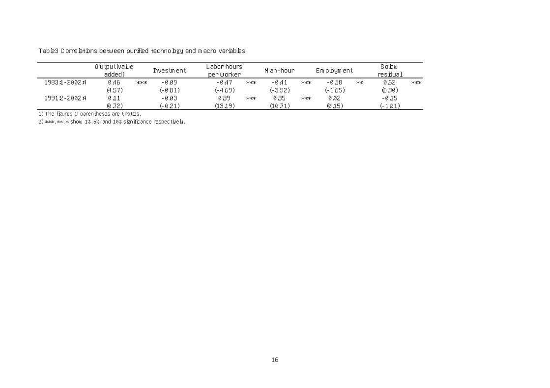
Table3 Correlations between purified technology and macro variables

Output(valueadded)

InvestmentLabor hoursper worker

Man-hour EmploymentSolowresidual

1983:1-2002:4 0.46 *** -0.09 -0.47 *** -0.41 *** -0.18 ** 0.62 ***(4.57) (-0.81) (-4.69) (-3.92) (-1.65) (6.90)

1991:2-2002:4 0.11 -0.03 0.89 *** 0.85 *** 0.02 -0.15(0.72) (-0.21) (13.19) (10.71) (0.15) (-1.01)

1) The figures in parentheses are t ratios.

2) ***, **, * show 1%, 5%, and 10% significance respectively.

16

Table4 Test of unit root in purified technology

ADF test Phillips Perron test1983:2-2002:4 -13.57066 *** -13.3311 ***1991:3-2002:4 -3.5070 *** -12.9505 ***1) *** implies that level in purified technology rejects null hypothesis of a unit root.

17

Table5 Regression on current and lagged purified technology1983:3-2002:4

∆v ∆j ∆h ∆nh ∆n

coefficientstandarderror

coefficientstandarderror

coefficientstandarderror

coefficientstandarderror

coefficientstandarderror

C 0.50 0.24 ** 1.95 1.03 * -0.13 0.24 0.23 0.35 0.03 0.03∆θ 0.43 0.10 *** -0.21 0.45 -0.27 0.11 ** -0.37 0.16 ** -0.01 0.01

∆θ(-1) 0.01 0.12 0.50 0.47 0.06 0.12 0.13 0.17 0.01 0.01

∆θ(-2) -0.11 0.11 0.05 0.46 0.12 0.12 0.05 0.16 0.00 0.01

∆v(-1) -0.24 0.12 **

∆v(−2) 0.08 0.12

∆j(-1) -0.59 0.12 ***

∆j(-2) -0.15 0.12

∆h(-1) -0.76 0.12 ***

∆h(-2) -0.05 0.11

∆nh(-1) -0.73 0.12 ***

∆nh(-2) -0.18 0.11

∆n(-1) 0.48 0.11 ***

∆n(-2) 0.33 0.12 ***

adj.R*R 0.23 0.26 0.63 0.56 0.56D.W. stat. 2.04 1.98 2.12 2.06 2.04AIC 1.44 4.45 1.60 -2.62 -2.66SBIC 1.63 4.63 1.78 -2.44 -2.48

1) Figures in parenthesis are standard deviations2) ***, **, * show 1%, 5%, and 10% significance respectively.

18

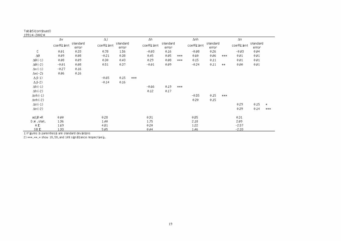
Table5(continued)1991:4-2002:4

∆v ∆j ∆h ∆nh ∆n

coefficientstandarderror

coefficientstandarderror

coefficientstandarderror

coefficientstandarderror

coefficientstandarderror

C 0.01 0.33 0.78 1.56 -0.03 0.16 -0.08 0.26 -0.03 0.04∆θ 0.09 0.08 -0.21 0.38 0.45 0.05 *** 0.60 0.06 *** 0.01 0.01

∆θ(-1) 0.08 0.09 0.30 0.43 0.29 0.08 *** 0.15 0.11 0.01 0.01

∆θ(-2) -0.01 0.08 0.51 0.37 -0.01 0.09 -0.24 0.11 ** 0.00 0.01

∆v(-1) -0.27 0.16

∆v(−2) 0.06 0.16

∆j(-1) -0.65 0.15 ***

∆j(-2) -0.14 0.16

∆h(-1) -0.66 0.19 ***

∆h(-2) 0.12 0.17

∆nh(-1) -0.55 0.15 ***

∆nh(-2) 0.20 0.15

∆n(-1) 0.29 0.15 *

∆n(-2) 0.39 0.14 ***

adj.R*R 0.00 0.28 0.91 0.85 0.31D.W. stat. 1.96 1.40 1.75 2.18 2.09AIC 1.69 4.81 0.20 1.22 -2.57SBIC 1.93 5.05 0.44 1.46 -2.33

1) Figures in parenthesis are standard deviations2) ***, **, * show 1%, 5%, and 10% significance respectively.

19

Table6 Granger Causality Tests1983:1-2002:4

F-Statistic∆θ→∆h 0.766

∆θ→∆nh 1.201

∆θ→∆n 0.339

∆m→∆h 0.249

∆m→∆nh 1.253

∆m→∆n 2.830 *

1991:2-2002:4F-Statistic

∆θ→∆h 7.336 ***

∆θ→∆nh 1.232

∆θ→∆n 0.164

∆m→∆h 0.656

∆m→∆nh 0.170

∆m→∆n 0.6011) ***, **, * shows that non-existence of Granger causality is rejected at 1%, 5%, and 10% significance level, respectively.

20

Table7 Regression on current and lagged purified technology including dispersion measure1983:3-2002:4

∆h ∆nh ∆n

coefficientstandarderror

coefficientstandarderror

coefficientstandarderror

C -0.72 0.85 -0.40 1.20 0.12 0.11∆θ -0.25 0.11 ** -0.35 0.16 ** -0.02 0.01

∆θ(-1) 0.07 0.12 0.15 0.16 0.00 0.01

∆θ(-2) 0.12 0.11 0.04 0.16 0.00 0.01

∆h(-1) -0.81 0.13 ***

∆h(-2) -0.04 0.13

∆nh(-1) -0.75 0.13 ***

∆nh(-2) -0.10 0.13

∆n(-1) 0.49 0.12 ***

∆n(-2) 0.32 0.12 ***disp -0.25 0.25 -0.22 0.36 0.01 0.03disp(-1) 0.53 0.26 ** 0.92 0.37 ** -0.05 0.03disp(-2) -0.05 0.24 -0.46 0.35 0.00 0.03

adj.R*R 0.64 0.54 0.56D.W. stat. 2.13 2.32 2.04AIC 1.61 2.32 -2.59SBIC 1.89 2.59 -2.31

1991:4-2002:4∆h ∆nh ∆n

coefficientstandarderror

coefficientstandarderror

coefficientstandarderror

C -0.68 0.67 -2.29 1.21 * -0.02 0.21∆θ 0.36 0.04 *** 0.42 0.08 *** 0.01 0.01

∆θ(-1) 0.21 0.07 *** 0.15 0.10 0.00 0.02

∆θ(-2) 0.02 0.07 -0.19 0.10 * -0.01 0.01

∆h(-1) -0.88 0.17 ***

∆h(-2) -0.09 0.16

∆nh(-1) -0.75 0.19 ***

∆nh(-2) 0.12 0.19

∆n(-1) 0.30 0.16 *

∆n(-2) 0.34 0.16 **disp -0.21 0.09 ** -0.18 0.18 -0.01 0.03disp(-1) 0.10 0.09 0.53 0.18 *** 0.01 0.03disp(-2) 0.24 0.09 *** 0.12 0.19 0.00 0.03

adj.R*R 0.94 0.88 0.26D.W. stat. 1.99 2.05 2.08AIC -0.15 1.06 -2.45SBIC 0.21 1.42 -2.09

1) Figures in parenthesis are standard deviations2) ***, **, * show 1%, 5%, and 10% significance respectively.

21

Figure1 Accumulated impulse response of output(1983:3-2002:4)

-0.2

0.0

0.2

0.4

0.6

0.8

1.0

1.2

1 2 3 4 5 6 7 8 9 10

22

Figure2 Accumulated impulse response of labor hours per person(1983:3-2002:4)

-0.8

-0.4

0.0

0.4

0.8

1.2

1 2 3 4 5 6 7 8 9 10

23

Figure3 Accumulated impulse response of total man-hour(1983:3-2002:4)

-0.8

-0.4

0.0

0.4

0.8

1.2

1 2 3 4 5 6 7 8 9 10

24

Figure4 Accumulated impulse response of employment(1983:3-2002:4)

-4

0

4

8

12

16

1 2 3 4 5 6 7 8 9 10

25

Figure5 Accumulated impulse response of investment(1983:3-2002:4)

-0.8

-0.4

0.0

0.4

0.8

1.2

1 2 3 4 5 6 7 8 9 10

26

Figure6 Accumulated impulse response of output(1991:4-2002:4)

-0.4

0.0

0.4

0.8

1.2

1 2 3 4 5 6 7 8 9 10

27

Figure7 Accumulated impulse response of labor hours per person(1991:4-2002:4)

-1.2

-0.8

-0.4

0.0

0.4

0.8

1.2

1 2 3 4 5 6 7 8 9 10

28

Figure8 Accumulated impulse response of total man-hour(1991:4-2002:4)

-0.2

0.0

0.2

0.4

0.6

0.8

1.0

1.2

1 2 3 4 5 6 7 8 9 10

29

Figure9 Accumulated impulse response of employment(1991:4-2002:4)

-4

-2

0

2

4

6

8

10

1 2 3 4 5 6 7 8 9 10

30

Figure10 Accumulated impulse response of investment(1991:4-2002:4)

-0.8

-0.4

0.0

0.4

0.8

1.2

1 2 3 4 5 6 7 8 9 10

31

Table A-1 Industry Classification Table

Classification in JapanStandard Industrial

Classification (The 10thRevised Edition)

1 Construction 9,10,112 Manufacture of Food Products 12, 13 3 Manufacture of Textiles 144 Manufacture of Wearing Apparel and Other Textile Products 155 Manufacture of Lumber and Wood Products 166 Manufacture of Pulp , Paper and Paper Products 187 Manufacture of Publishing and Printing 198 Manufacture of Chemicals and Chemical Products 209 Manufacture of Petroleum and Coal Products 2110 Manufacture of Stone, Clay and Glass Products 2511 Manufacture of Steel 2612 Manufacture of Non-Ferrous Metals 2713 Manufacture of Metal Products 2814 Manufacture of General Machinery Equipment 2915 Manufacture of Electrical Machinery 3016 Manufacture of Transportation Equipment 3117 Manufacture of Precision Machinery and Equipment 3218 Manufacture of Ships 3119 Other Manufacturing 17,22,23,24,33,3420 Wholesale 48,49,50,51,52,5321 Retail 54,55,56,57,58,59,60,6122 Real Estate 70,7123 Land Transportation 39,40,4124 Water Transportation 4225 Other Transportation and communication 43,44,45,46,4726 Electricity 3527 Gas, Waterworks 36,37,3828 Services for Business 79,82,83,8629 Inns, Other Lodging 7530 Services for Individuals 72,73,7431 Movies, Entertainment 76,8032 Broadcasting 8133 Other Services 77,78,84,87,88,89,91,92,95

Classification in the Financial Statements Statistics ofCorporations

32

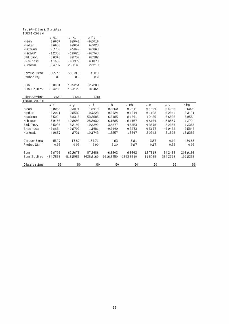
TableA-2 Basic Statistics1983:1-2002:4

⊿yi ⊿xi ⊿hi Mean 0.0034 0.0040 -0.0010 Median 0.0055 0.0054 0.0023 Maximum 0.7752 0.5842 0.0809 Minimum -1.2960 -1.0028 -0.0948 Std. Dev. 0.0942 0.0757 0.0382 Skewness -1.1659 -0.7372 -0.1878 Kurtosis 30.4787 25.7105 2.0213

Jarque-Bera 83657.0 56973.6 120.9 Probability 0.0 0.0 0.0

Sum 9.0481 10.5251 -2.7283 Sum Sq. Dev 23.4295 15.1120 3.8461

Observations 2640 2640 26401983:1-2002:4

⊿θ ⊿y ⊿j ⊿h ⊿nh ⊿n ⊿v disp Mean 0.0059 0.7871 1.0919 -0.0860 0.0871 0.1599 0.4280 2.6002 Median -0.2011 0.8530 0.7228 0.0924 -0.1014 0.1152 0.2944 2.3171 Maximum 5.5074 8.4315 53.2685 6.0185 8.1591 1.2435 5.6926 8.9554 Minimum -9.9192 -10.8692 -28.3030 -6.1685 -6.1157 -0.6104 -5.8867 1.1724 Std. Dev. 2.5025 3.2190 10.3292 3.5877 4.5053 0.3878 2.2339 1.1353 Skewness -0.4654 -0.6700 1.1981 -0.0490 0.3073 0.5177 -0.0463 2.5846 Kurtosis 4.9657 4.8721 10.1743 1.8257 1.8847 3.0043 3.1808 13.8382

Jarque-Bera 15.77 17.67 190.71 4.63 5.41 3.57 0.14 480.63 Probability 0.00 0.00 0.00 0.10 0.07 0.17 0.93 0.00

Sum 0.4702 62.9676 87.3486 -6.8802 6.9642 12.7919 34.2433 208.0199 Sum Sq. Dev 494.7533 818.5950 8428.6160 1016.8750 1603.5210 11.8798 394.2219 101.8236

Observations 80 80 80 80 80 80 80 80

33

TableA-2(continued)1991:2-2002:4

⊿yi ⊿xi ⊿hi Mean 0.0001 0.0009 -0.0003 Median 0.0018 0.0030 0.0033 Maximum 0.7752 0.5574 0.0809 Minimum -1.2960 -1.0028 -0.0948 Std. Dev. 0.0945 0.0751 0.0378 Skewness -1.0992 -0.9411 -0.2888 Kurtosis 33.5540 31.3200 2.1241

Jarque-Bera 60642.7 52059.7 71.1 Probability 0.0 0.0 0.0

Sum 0.1782 1.4663 -0.4460 Sum Sq. Dev 13.8486 8.7504 2.2158

Observations 1551 1551 15511991:2-2002:4

⊿θ ⊿y ⊿j ⊿h ⊿nh ⊿n ⊿v disp Mean -0.1059 0.2594 0.3231 -0.0237 0.0013 0.0139 0.0268 4.4412 Median -0.1955 0.3536 0.4291 0.6843 0.2615 0.0000 0.1371 4.3141 Maximum 10.5692 7.5769 53.2685 6.0143 8.1505 1.2435 5.6926 9.7683 Minimum -10.4180 -7.5942 -28.3030 -6.1325 -5.9453 -0.6104 -4.2958 1.5027 Std. Dev. 4.8403 3.0304 12.1235 3.4752 4.4657 0.3688 2.1466 2.0608 Skewness 0.0622 -0.2750 1.3717 -0.1433 0.3318 1.2214 0.3048 0.6047 Kurtosis 2.2516 3.7959 9.4109 1.8469 1.8644 5.2810 3.1100 2.5550

Jarque-Bera 1.13 1.83 95.22 2.76 3.39 21.88 0.75 3.25 Probability 0.57 0.40 0.00 0.25 0.18 0.00 0.69 0.20

Sum -4.9762 12.1904 15.1859 -1.1116 0.0594 0.6511 1.2607 208.7359 Sum Sq. Dev 1077.6910 422.4363 6761.0250 555.5356 917.3680 6.2582 211.9619 195.3550

Observations 47 47 47 47 47 47 47 47

34