Do Mutual Funds Manipulate Star Ratings? Evidence from ...

Do Mutual Funds Manipulate Star Ratings?

Evidence from Portfolio Pumping

Sanghyun (Hugh) Kim∗

December 31, 2020

Abstract

This paper reveals that mutual fund managers manipulate Morningstar ratings by in-flating their month-end portfolio values when they are likely to finish the month nearrating cutoffs. This star rating manipulation is more pronounced among funds withgreater incentives and abilities to pump their portfolios and manipulate star ratings.Following heightened regulatory scrutiny, portfolio pumping to manipulate star ratingshas largely migrated from quarter/year-ends to less prominent month-ends. Improv-ing star ratings, portfolio pumping increases fund flows, especially in the month of arating upgrade. Placebo tests exploiting the June 2002 change in Morningstar’s ratingmethodology yield expected null effects.

JEL classification: G23, G24, G28, K22

Keywords: Morningstar ratings, managerial incentives, mutual funds, portfolio pumping,performance manipulation

∗Hugh Kim ([email protected]) is at the University of Texas at Dallas, 800 W. Campbell Road,Richardson, TX 75080. I thank Vikram Nanda, Kelsey Wei, Umit Gurun, Alessio Saretto, Qinghai Wang,Munhee Han, Rose Liao, Harold Zhang, Nina Baranchuk, Steven Xiao, Yexiao Xu, Feng Zhao, KyounghunBae (discussant), Anna von Reibnitz (discussant), Jun Chen, Timothy Riddiough, Justin Birru (discussant),Ryan Davies, Eduard Inozemtsev (discussant), Darwin Choi, Philip Dybvig, Byoung Uk Kang, seminarparticipants at the University of Texas at Dallas, and conference participants at the Conference on Asia-Pacific Financial Markets 2019, Australasian Finance and Banking Conference 2019, New Zealand FinanceMeeting 2019, Northern Finance Association (NFA) Annual Conference 2020, and Financial ManagementAssociation (FMA) Annual Meeting 2020 for helpful comments.

“We are all in the gutter, but some of us are looking at the stars.”

– Oscar Wilde

1 Introduction

Since its introduction in 1985, Morningstar’s five-star rating system has become widely ac-

cepted in the mutual fund industry (Del Guercio and Tkac (2008)).1 Unlike performance measures

commonly used in academia (e.g., Jensen (1969), Carhart (1997), Daniel et al. (1997)), Morningstar

star ratings offer less sophisticated investors a simple and intuitive tool to use to allocate their cap-

ital across mutual funds. Prior studies find that discrete star ratings have a powerful influence on

fund flows, independent of the underlying continuous performance metric used to rank funds (Del

Guercio and Tkac (2008), Reuter and Zitzewitz (2015)). Evans and Sun (Forthcoming) show that

mutual fund investors use simple heuristics such as star ratings, rather than asset-pricing models,

for risk adjustment. Ben-David et al. (2019) further argue that star ratings explain mutual fund

investors’ behavior better than asset pricing models, concluding that star ratings are the main

determinant of capital allocation across mutual funds.

Whereas how star ratings influence the behavior of mutual fund investors is well-documented,

little is known about how star ratings distort the incentives of mutual fund managers. In this paper,

I argue that the closer fund rankings are to rating cutoffs, the greater the incentive to inflate the

underlying performance metric that Morningstar uses to determine star ratings. The incentive

to manipulate star ratings arises because even a small increase in fund rankings (such as going

from 89th percentile to 90th percentile) can induce discrete changes in star ratings (such as going

from four stars to five stars), which in turn leads to a large jump in fund flows (Reuter and

Zitzewitz (2015)). Consistent with my prediction, I find strong evidence that U.S. equity mutual1Mutual fund share classes are rated at the end of each month on a scale of one star (lowest) to five stars

(highest) on the basis of Morningstar Risk-Adjusted Returns (MRAR). The top 10% of funds receive fivestars, the next 22.5% four stars, the middle 35% three stars, the next 22.5% two stars, and the bottom 10%one star, approximately following a normal distribution.

1

fund managers manipulate star ratings by inflating their month-end portfolio values when they are

likely to finish the month in the vicinity of rating thresholds.

At the end of every month, mutual fund share classes are rated by Morningstar on the basis of

Morningstar Risk-Adjusted Returns (MRAR) over the prior three, five, and ten years, depending on

data availability. “Overall” star ratings are then determined by taking weighted-averages of three,

five, and ten-year star ratings, rounded to the nearest integer value.2 Following the literature, my

paper focuses on overall star ratings, which are most prominently featured by Morningstar as well

as mutual fund companies.

On June 30, 2002, Morningstar implemented a major change to its star rating methodology.

In addition to changing the risk adjustment process, Morningstar refined its peer groups used to

rank mutual funds.3 Incorporating the June 2002 change, I rank mutual fund share classes each

month on the basis of MRAR computed following Blume (1998) until May 2002 and Morningstar

(2016) starting in June 2002, relative to the peer groups Mornigstar used before and after the

change, respectively. To estimate rankings prior to monthly rating updates, I use trailing returns

over the prior 36, 60, and 120 months, depending on data availability, that are cumulative only

up to the second-to-last trading day of the month in the computation of MRAR. Then, I compute

“overall” percentile rankings by taking weighted-averages of three, five, and ten-year percentile

rankings. Last, I compute the distance to a rating threshold as the distance between overall

percentile rankings and the nearest rating threshold.2Mutual fund share classes less than three years old are not rated. Share classes at least three years old

but less than five years old are rated based only on three-year star ratings. Share classes at least five yearsold but less than ten years old are rated based on three-year star ratings (40 percent weight) and five-yearstar ratings (60 percent weight). Share classes at least ten years old are rated based on three-year starratings (20 percent weight), five-year star ratings (30 percent weight), and ten-year star ratings (50 percentweight).

3Morningstar started raking U.S. equity mutual funds within nine (three-by-three) investment style cate-gories (market-cap interacted with value/growth), whereas all U.S. equity mutual funds were ranked withina single category prior to the change. The revised formula of the MRAR measures the annualized estimateof the certainty equivalent geometric excess return for an investor with CRRA utility (Morningstar (2016)),whereas the older version of the MRAR adjusts for the downside risk (See Blume (1998) for a detailedexplanation of the algorithm used to calculate the MRAR).

2

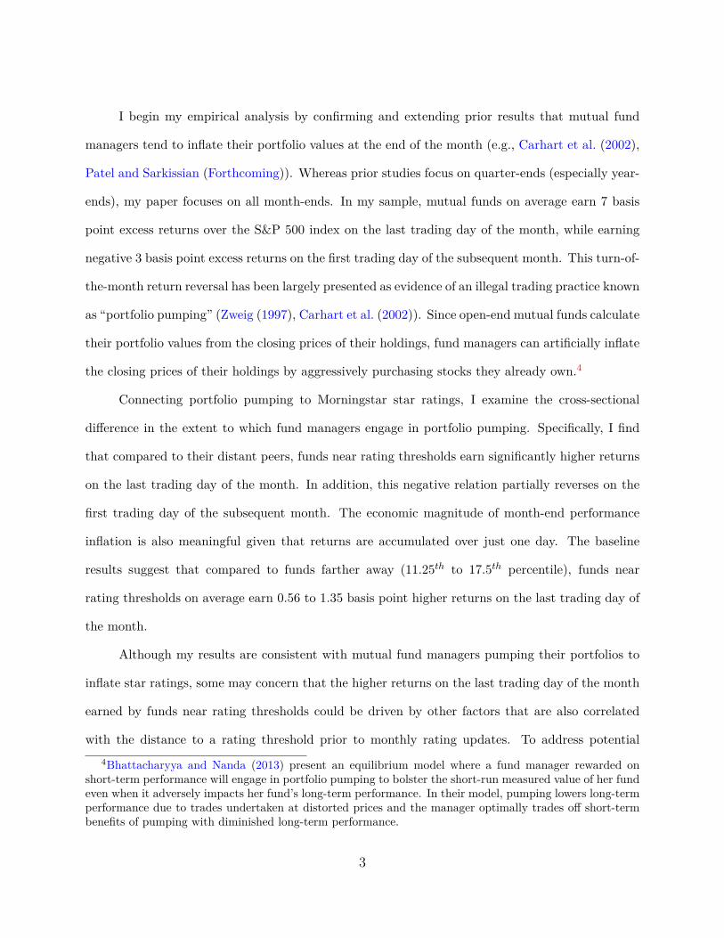
I begin my empirical analysis by confirming and extending prior results that mutual fund

managers tend to inflate their portfolio values at the end of the month (e.g., Carhart et al. (2002),

Patel and Sarkissian (Forthcoming)). Whereas prior studies focus on quarter-ends (especially year-

ends), my paper focuses on all month-ends. In my sample, mutual funds on average earn 7 basis

point excess returns over the S&P 500 index on the last trading day of the month, while earning

negative 3 basis point excess returns on the first trading day of the subsequent month. This turn-of-

the-month return reversal has been largely presented as evidence of an illegal trading practice known

as “portfolio pumping” (Zweig (1997), Carhart et al. (2002)). Since open-end mutual funds calculate

their portfolio values from the closing prices of their holdings, fund managers can artificially inflate

the closing prices of their holdings by aggressively purchasing stocks they already own.4

Connecting portfolio pumping to Morningstar star ratings, I examine the cross-sectional

difference in the extent to which fund managers engage in portfolio pumping. Specifically, I find

that compared to their distant peers, funds near rating thresholds earn significantly higher returns

on the last trading day of the month. In addition, this negative relation partially reverses on the

first trading day of the subsequent month. The economic magnitude of month-end performance

inflation is also meaningful given that returns are accumulated over just one day. The baseline

results suggest that compared to funds farther away (11.25th to 17.5th percentile), funds near

rating thresholds on average earn 0.56 to 1.35 basis point higher returns on the last trading day of

the month.

Although my results are consistent with mutual fund managers pumping their portfolios to

inflate star ratings, some may concern that the higher returns on the last trading day of the month

earned by funds near rating thresholds could be driven by other factors that are also correlated

with the distance to a rating threshold prior to monthly rating updates. To address potential4Bhattacharyya and Nanda (2013) present an equilibrium model where a fund manager rewarded on

short-term performance will engage in portfolio pumping to bolster the short-run measured value of her fundeven when it adversely impacts her fund’s long-term performance. In their model, pumping lowers long-termperformance due to trades undertaken at distorted prices and the manager optimally trades off short-termbenefits of pumping with diminished long-term performance.

3

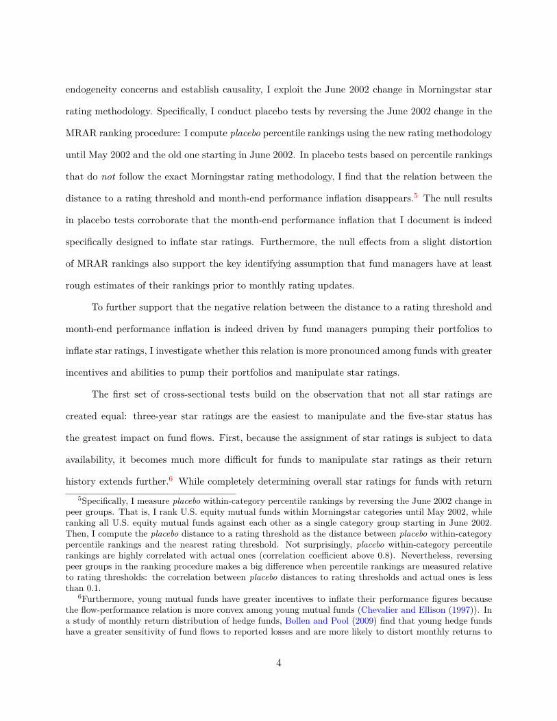
endogeneity concerns and establish causality, I exploit the June 2002 change in Morningstar star

rating methodology. Specifically, I conduct placebo tests by reversing the June 2002 change in the

MRAR ranking procedure: I compute placebo percentile rankings using the new rating methodology

until May 2002 and the old one starting in June 2002. In placebo tests based on percentile rankings

that do not follow the exact Morningstar rating methodology, I find that the relation between the

distance to a rating threshold and month-end performance inflation disappears.5 The null results

in placebo tests corroborate that the month-end performance inflation that I document is indeed

specifically designed to inflate star ratings. Furthermore, the null effects from a slight distortion

of MRAR rankings also support the key identifying assumption that fund managers have at least

rough estimates of their rankings prior to monthly rating updates.

To further support that the negative relation between the distance to a rating threshold and

month-end performance inflation is indeed driven by fund managers pumping their portfolios to

inflate star ratings, I investigate whether this relation is more pronounced among funds with greater

incentives and abilities to pump their portfolios and manipulate star ratings.

The first set of cross-sectional tests build on the observation that not all star ratings are

created equal: three-year star ratings are the easiest to manipulate and the five-star status has

the greatest impact on fund flows. First, because the assignment of star ratings is subject to data

availability, it becomes much more difficult for funds to manipulate star ratings as their return

history extends further.6 While completely determining overall star ratings for funds with return5Specifically, I measure placebo within-category percentile rankings by reversing the June 2002 change in

peer groups. That is, I rank U.S. equity mutual funds within Morningstar categories until May 2002, whileranking all U.S. equity mutual funds against each other as a single category group starting in June 2002.Then, I compute the placebo distance to a rating threshold as the distance between placebo within-categorypercentile rankings and the nearest rating threshold. Not surprisingly, placebo within-category percentilerankings are highly correlated with actual ones (correlation coefficient above 0.8). Nevertheless, reversingpeer groups in the ranking procedure makes a big difference when percentile rankings are measured relativeto rating thresholds: the correlation between placebo distances to rating thresholds and actual ones is lessthan 0.1.

6Furthermore, young mutual funds have greater incentives to inflate their performance figures becausethe flow-performance relation is more convex among young mutual funds (Chevalier and Ellison (1997)). Ina study of monthly return distribution of hedge funds, Bollen and Pool (2009) find that young hedge fundshave a greater sensitivity of fund flows to reported losses and are more likely to distort monthly returns to

4

history of less than five years, three-year star ratings account for only a small faction (20 to 40

percent) of overall star ratings for funds with return history of at least five years. Second, Reuter

and Zitzewitz (2015) find that discontinuities in the flow-performance relation are greater at higher

rating cutoffs and greatest at the four/five-star cutoff.7 Thus, funds around the four/five-star rating

cutoff should have the strongest incentive to inflate star ratings. Consistent with my cross-sectional

predictions, I find that star rating manipulation through portfolio pumping is more pronounced

among younger funds with return history of less than five years and funds around the four/five-star

rating cutoff.

The next set of cross-sectional tests build on the prior literature on portfolio pumping. First,

Carhart et al. (2002) argue that if fund managers are indeed “marking up” their funds’ portfolio

values, portfolio pumping should be more pronounced among small-cap funds because the closing

prices of less liquid stocks would presumably be easier to influence. Second, Patel and Sarkissian

(Forthcoming) argue that peer effects among teams such as the presence of peer monitoring and

joint monetary incentives are effective in deterring fund managers from engaging in illegal trading

activities such as portfolio pumping. Consistent with these prior studies, I find that the negative

relation between the distance to a rating threshold and month-end performance inflation is more

pronounced among small-cap funds and single-managed funds, weakening as the size of management

team increases.

After the initial results of Carhart et al. (2002) drew a great deal of attention from regulators,

academics, and practitioners, the U.S. Securities and Exchange Commission (SEC) began to inves-

tigate suspicious trading activities (Duong and Meschke (2020)). Recent studies note that following

heightened regulatory attention, portfolio pumping has become more evasive (e.g., Hu et al. (2014),

Wang (2019)). To examine whether star rating manipulation through portfolio pumping has be-

come more evasive, I conduct sub-period tests by splitting my sample around the June 2002 change

temporarily avoid reporting losses.7Similarly, Del Guercio and Tkac (2008) find that among all rating changes, upgrades from four to five

stars have the greatest impact on fund flows.

5

in Morningstar rating methodology, which approximately coincides with the publication of Carhart

et al. (2002). My sub-period tests reveal that portfolio pumping to manipulate star ratings has

largely migrated from quarter/year-ends to less prominent month-ends, presumably to evade regu-

latory attention. In the early period, star rating manipulation through portfolio pumping was more

pronounced at quarter/year-ends, consistent with the prior literature’s focus on portfolio pumping

at quarter-ends (especially year-ends) (e.g., Carhart et al. (2002), Hu et al. (2014)). In the recent

period, however, the negative relation between the distance to a rating threshold and month-end

performance inflation is more pronounced at month-ends that are not quarter/year-ends, whereas

it has become insignificant at quarter/year-ends.

My results thus far suggest that fund managers manipulate star ratings by inflating month-

end portfolio values, especially when their funds are likely to finish the month near rating cutoffs.

Portfolio pumping, however, could lower performance figures for the next month because a large

fraction of gains on the last trading day of the month dissipates on the first trading day of the

subsequent month. Theoretical studies also suggest that portfolio pumping, while improving a

fund’s short-term values, may hurt its long-term values (e.g., Bhattacharyya and Nanda (2013)).

To better understand what fund managers gain from engaging in portfolio pumping, I examine

the effect of star rating manipulation on fund flows. Doing so, however, poses an empirical challenge

because changes in star ratings (especially upgrades) have a large impact on fund flows (Del Guercio

and Tkac (2008)) and a rating upgrade is at most only partially due to portfolio pumping. To tease

out the effect of a rating upgrade on fund flows that can attributable to portfolio pumping, I exploit

a two-stage least squares (2SLS) estimation. In the first stage, I find that month-end performance

inflation is associated with a higher probability of a rating upgrade at the end of the month.

Rating upgrades driven by portfolio pumping, however, are more likely to be offset by immediate

downgrades in the subsequent months due to the return reversal around the turn of the month.

Nevertheless, pumping funds can capture additional fund flows in the month of a rating upgrade

without any significant punishment in the subsequent months. In the second stage, I find that star

6

rating manipulation driven by month-end performance inflation significantly increases future fund

flows, especially in the month of a rating upgrade.

The remainder of my paper is organized as follows. In the next section, I discuss the contri-

bution of my paper in the context of related literature. Section 3 provides institutional details on

Morningstar ratings pertaining to my paper. Section 4 introduces my data sets and describes how

I construct key variables used in the my analysis. Section 5 presents evidence of star rating ma-

nipulation. Section 6 examines the effects of star rating manipulation through portfolio pumping.

Section 7 concludes.

2 Related Literature

To the best of my knowledge, my paper is the first to link portfolio pumping to Morningstar

star ratings, thereby contributing to several strands of literature.

First, my paper sheds new light on how star ratings can distort managerial incentives of

mutual funds. The prior literature often focuses on the convex flow-performance relation (Ippolito

(1992), Sirri and Tufano (1998)) to explain mutual funds’ behavior in various settings (e.g., Cheva-

lier and Ellison (1997)). Along this line, Carhart et al. (2002) use the convex flow-performance

relation, which becomes increasingly steeper toward the top end of the performance spectrum, to

propose that the “leaning-for-the-tape” effect is driving portfolio pumping.8 Prior studies, how-

ever, offer little insight on mutual funds’ behavior in less steep regions of the flow-performance

relation. My paper complements the prior literature on mutual funds’ managerial incentives by

connecting it to a growing literature on Morningstar ratings. In particular, Reuter and Zitzewitz

(2015) show that mutual fund investors’ heavy reliance on star ratings creates discontinuities at

rating thresholds in the flow-performance relation. My paper shows that such discontinuities in8However, the result of Carhart et al. (2002) that the magnitude of portfolio pumping is more severe

among high-performing funds is sample-specific. Patel and Sarkissian (Forthcoming) find that the magnitudeof portfolio pumping is more severe among low-performing funds in their full sample from 1992 to 2015 andalmost identical for both high-performing and low-performing funds in their reduced sample ending in 2010.

7

the flow-performance relation can give mutual fund managers powerful incentives to inflate their

performance figures when their performance rankings are near rating cutoffs.

Second, my paper contributes to the literature on portfolio pumping. Departing from the

prior literature that focuses on an aggregate level of portfolio pumping among equity mutual funds

(and hedge funds) (e.g., Carhart et al. (2002), Ben-David et al. (2013), Hu et al. (2014)), my paper

focuses on when mutual fund managers pump their portfolios. That is, rather than comparing

funds’ daily returns around the turn of the calendar year and quarters with daily returns for the

rest of the year, I compare daily returns of funds close to rating thresholds with daily returns of

funds farther away from rating thresholds around the turn of each calendar month. Funds that are

close to (or farther away from) rating cutoffs change frequently because within-category rankings

are based on past performance on a rolling basis. In addition, while prior studies tend to focus

on portfolio pumping at quarter-ends (especially year-ends), this paper focuses on the tournament

among fund managers at a higher frequency, consistent with Del Guercio and Tkac (2008) who find

that the flow response to rating changes occurring at year-end is not different from that of other

months.

Since portfolio pumping is an illegal trading practice, pumping managers would likely take

caution. Indeed, my findings suggest that mutual fund managers engage in portfolio pumping

infrequently and irregularly, and only do so when shifting performance from the next month to the

current month is likely to result in the largest benefits. After the results of Carhart et al. (2002)

were first disseminated in 2000, the SEC began to investigate suspicious trading activities. Duong

and Meschke (2020) document a reduced level of portfolio pumping since late 2000 and other recent

studies find that portfolio pumping has become more evasive. Hu et al. (2014) find that in their

sample of Abel Noser clients from 1999 to 2010, year-end price inflation derives from depressed

institutional selling rather than aggressive institutional buying. Wang (2019) shows that non-top-

performing funds pump the portfolios held by top-performing funds in their own fund family at

quarter-ends, but only after 2002. Consistent with these studies, my paper shows that following

8

heightened regulatory scrutiny prompted by Carhart et al. (2002), portfolio pumping induced by

star ratings has largely migrated from quarter/year-ends to less prominent month-ends.

Third, my paper contributes to a growing literature on Morningstar ratings of mutual funds.

Del Guercio and Tkac (2008) show that in an event study setting, rating changes have a significant

impact on fund flows, independent of the underlying continuous performance measures. Exploiting

a regression discontinuity design, Reuter and Zitzewitz (2015) find that a large fraction of the

difference in future fund flows received by five- and one-star funds represents a causal effect of

the difference in star ratings on fund flows. Evans and Sun (Forthcoming) show that mutual

fund investors use simple heuristics such as star ratings, rather than asset-pricing models, for risk

adjustment. Ben-David et al. (2019) further argue that star ratings explain mutual fund investors’

behavior much better than any asset pricing models. These recent studies cast doubt on the

premise that mutual fund investors (most of whom are retail investors) are sophisticated enough

to use asset pricing models in their capital allocation across mutual funds, as suggested by Berk

and van Binsbergen (2016) and Barber et al. (2016). My paper weighs in on this debate by taking

the perspective of mutual fund managers and showing that mutual fund managers themselves also

respond strongly to star ratings.

Last, my paper adds to the literature on managerial incentives that exist around various

thresholds. Bollen and Pool (2009) uncover a discontinuity in the distribution of hedge fund monthly

returns at zero and present evidence that hedge fund managers tend to overstate monthly returns

to temporarily avoid reporting losses. Lee et al. (2019) show that mutual fund managers with

performance-based contracts and mid-year performance close to their announced benchmarks tend

to increase their portfolio risk in the second part of the year. In a corporate setting, Begley (2015)

finds that firms close to key Debt/EBITDA thresholds are more likely to reduce R&D and SG&A

expenditures, presumably to boost EBITDA and receive higher credit ratings, especially prior to

bond issuance.

9

3 Morningstar Ratings

At the end of each month, mutual fund share classes are rated by Morningstar on an integer

scale of one star (the lowest rating) to five stars (the highest rating). Star ratings are determined

by within-category rankings of Morningstar Risk-Adjusted Return (MRAR) over the prior three,

five, and ten years, depending on data availability. MRAR has gone through several methodological

changes over time. In October 2016, Morningstar removed load adjustment from the calculation of

star ratings. In June 2002, Morningstar changed the risk-adjustment process in the computation

of MRAR, which is currently defined as follows (Morningstar (2016)):

MRAR(γ) =[

1T

T∑t=1

(1 + ERt)−γ]− 12

γ

− 1, γ > −1, γ 6= 0 (1)

where ERt is the geometric excess return over the risk-free rate in month t, γ is the risk-aversion

coefficient, and T is the number of months in the time period. Morningstar sets γ = 2 in the

calculation of star ratings, arguing that doing so results in fund rankings that are consistent with

the risk tolerances of typical retail investors.9 Prior to the June 2002 change, Morningstar used

a rather complicated process of adjusting for risk. I refer interested readers to Sharpe (1998) and

Blume (1998) for detailed explanations of the risk-adjustment process Morningstar used until May

2002.

In addition to the risk-adjustment process, Morningstar refined its peer groups used to rank

mutual funds in June 2002. Specifically, Morningstar started raking U.S. equity mutual funds

within its nine (three-by-three style box) categories along the size dimension (small, mid-cap, or

large) and value dimension (value, blend, or growth), whereas all U.S. equity mutual funds, as a

single category group, were ranked against each other until May 2002. On the basis of within-9Morningstar explains that MRAR is motivated by expected utility theory. To see this, let ERCE(γ)

denote the certainty equivalent geometric excess return with a risk-aversion coefficient of γ. With a powerutility function, u(1 +ERCE(γ)) = E[u(1 +ER)] becomes (1 +ERCE)−γ = E[(1 +ER)−γ ], γ > −1, γ 6= 0.Thus, MRAR(γ) is the annualized estimate of the certainty equivalent geometric excess return, ERCE(γ) =E[(1 + ER)−γ ]−

1γ − 1. See Morningstar (2016) for further details.

10

category rankings of MRAR, the top 10% of mutual fund share classes receive five stars, the next

22.5% four stars, the middle 35% three stars, the next 22.5% two stars, and the bottom 10% receive

one star, approximately following a normal distribution.

Overall star ratings are determined by the weighted averages of three, five, and ten-year star

ratings, depending data availability, rounded to the nearest integer value. Share classes less than

three years old are not rated. Share classes at least three years old but less than five years old are

rated based only on three-year star ratings. Share classes at least five years old but less than ten

years old are rated based on three-year star ratings (40 percent weight) and five-year star ratings

(60 percent weight). Share classes at least ten years old are rated based on three-year star ratings

(20 percent weight), five-year star ratings (30 percent weight), and ten-year star ratings (50 percent

weight).

Table 1 shows the transition matrix where each element in row i and column j represents

the probability of a mutual fund share class receiving rating j at the end of month t conditional

on its receiving rating i at the end of month t − 1. More than 10% of mutual fund share classes

experience changes in star ratings each month. Not surprisingly, ten-year star ratings are most

persistent, followed by five-year star ratings, and three-year star ratings are least persistent. Being

weighted averages, overall star ratings are more persistent than three-year star ratings, but less

persistent than five- and ten-year star ratings.

[Insert Table 1]

4 Data and Variable Construction

My primary data come from the survivorship-bias-free Morningstar Direct database, from

which I obtain data on returns, total net assets (TNA), Morningstar categories, star ratings, in-

ception dates, expense ratios, turnover ratios, index-fund indicators, and institutional share class

indicators for the period from 1990 to 2018. I obtain the risk-free rate from Fama-French Research

11

Factors.

To obtain within-category percentile rankings that are not contaminated by the outcomes of

the last trading session of the month, while replicating the rankings based on Morningstar Risk-

Adjusted Returns (MRAR) as closely as possible, I rank mutual fund share classes on the basis

of Sharpe ratio calculated using daily returns in excess of the risk-free rate over the prior three,

five, and ten-years, but only through the second-to-last trading day of the month. Sharpe (1998)

finds that ranking funds based on Sharpe ratio gives results that are very similar to ranking funds

based on MRAR in his sample from 1994 to 1996. MRAR, however, has gone through several

methodological changes over time. In June 2002, Morningstar changed the risk-adjustment process

in the computation of MRAR along with its peer groups used to rank mutual funds. In October

2016, Morningstar removed load adjustment from the calculation of star ratings. Nevertheless, I find

that ranking funds based on Sharpe ratio computed using daily returns without load adjustment

gives results that are very similar to ranking funds based on MRAR computed using monthly returns

and adjusted for sales charges throughout my sample. Specifically, I find that in untabulated results,

star ratings replicated based on Sharpe ratio computed using daily returns without load adjustment

are highly correlated with star ratings that are actually assigned by Morningstar in my sample from

1990 to 2018 (with a correlation coefficient over 83%). The 83% correlation is only slightly lower

than the 90% correlation reported by Evans and Sun (Forthcoming) when the authors replicate

star ratings by following the exact MRAR as closely as possible over the period from July 1999 to

May 2002.

Following the Morningstar rating methodology, I rank all U.S. equity mutual funds against

each other as a single category group until May 2002, whereas I rank funds within Morningstar’s

nine (three-by-three style box) categories along the size dimension (small, mid-cap, or large) and

value dimension (value, blend, or growth) starting in June 2002. Index funds are kept in the

ranking procedure to be consistent with Morningstar’s rating methodology, but excluded from the

main analysis because my paper focuses on actively-managed funds. Next, I compute overall within-

12

category percentile rankings by taking weighted-averages of three, five, and ten-year within-category

percentile rankings, consistent with how overall star ratings are determined. Share classes less than

three years old are excluded from the analysis because they are not rated. For share classes at least

three years old but less than five years old, overall rankings equal three-year rankings. For share

classes at least five years old but less than ten years old, overall rankings are weighted averages

of three-year rankings (40 percent weight) and five-year rankings (60 percent weight). For share

classes at least ten years old, overall rankings are weighted averages of three-year rankings (20

percent weight), five-year rankings (30 percent weight), and ten-year rankings (50 percent weight).

Finally, I compute the distance to a rating threshold as the distance between overall within-category

percentile rankings and the nearest rating threshold at the end of the second-to-last trading day of

the month. There are four rating thresholds dividing all mutual funds into five star ratings: 10th,

32.5th, 77.5th, and 90th percentiles. Mutual fund share classes above 95th percentile or below 5th

percentile are excluded from the analysis because they are closer to the corners of the performance

spectrum where no ratings are separated.

In my later analysis, I conduct placebo tests to corroborate that the negative relation between

the distance to a rating threshold and month-end NAV inflation is likely causal. To accomplish

this, I calculate placebo within-category percentile rankings by reversing the June 2002 change in

Morningstar’s rating methodology. Specifically, I rank mutual funds within Morningstar categories

prior to June 2002 while ranking all U.S. equity mutual funds against each other as a single category

group staring in June 2002. The placebo distance to a rating threshold is then computed based on

the placebo within-category percentile rankings.

Following the literature, I estimate fund flows for each mutual fund share class i during month

t as follows:

Flowi,t = TNAi,t − TNAi,t−1(1 +Ri,t)TNAi,t−1

(2)

13

where TNAi,t is the total net asset at the end of month t and Ri,t is the return during month t.

Table 2 provides the summary statistics on all variables used in the analysis throughout my paper.

All continuous variables are winsorized at 1% and 99%.

[Insert Table 2]

5 Star Rating Manipulation via Portfolio Pumping

I begin this section by presenting evidence that mutual fund managers manipulate star rat-

ings by inflating their month-end portfolio values, especially when their funds are likely to finish

the month in the vicinity of a rating threshold. To establish causality, I exploit the June 2002

change in Morningstar’s star rating methodology to corroborate that this month-end performance

manipulation is indeed designed to influence star ratings. Then, I show that star rating manip-

ulation through portfolio pumping is more pronounced among funds with greater incentives and

abilities to pump their portfolios and manipulate star ratings. Last, in sub-period tests, I uncover

that portfolio pumping to manipulate star ratings has become more evasive following heightened

regulatory scrutiny prompted by Carhart et al. (2002).

5.1 Distance to a Rating Threshold and Performance Inflation

The incentive to inflate month-end performance metrics is greater when funds are near rating

cutoffs because even a small increase in performance rankings (such as going from 89th percentile

to 90th percentile) can make discrete changes in star ratings (such as going from four stars to five

stars), which lead to a large jump in fund flows (Reuter and Zitzewitz (2015)). To test this star

rating manipulation hypothesis, I exploit the cross-sectional variation in the distance to a rating

threshold prior to rating updates at the end of the month.

As a first path, I visually inspect the relation between the distance to a rating threshold

measured at the end of the second-to-last trading day of the month and month-end performance

14

inflation. For each bin with the equal length of one-tenth of a percentile (i.e., 0.001) distance to a

rating threshold, I compute average daily returns of mutual fund share classes in excess of S&P 500

returns across each cross-section, weighted by the inverse of the number of share classes belonging

to the same fund. Then, I compute the time-series averages of the cross-sectional average excess

returns in the spirit of Fama and MacBeth (1973). In addition, I estimate the fitted curve from

the regression of the excess return on the squared distance to a rating threshold and report a 95%

confidence interval in the shaded area.

Figure 1 reports the results of this exploratory analysis. On the Y-axis are the average excess

returns on the last trading day of the month in Panel A and the average excess returns on the first

trading day of the next month in Panel B. Mutual funds, all across the board, tend to earn positive

excess returns on the last trading day of the month, whereas earning negative excess returns on

the next trading day. This turn-of-the-month return reversal, which has been widely presented as

a strong evidence of portfolio pumping, is consistent with the prior literature (e.g., Carhart et al.

(2002)).

Next, I turn to examining the cross-sectional difference in the extent to which mutual funds

engage in portfolio pumping. On the X-axis is the distance to a rating threshold prior to monthly

rating updates, measured at the end of the second-to-last trading day of the month. Panel A shows

that the distance to a rating threshold prior to monthly rating updates is negatively associated with

the excess return on the last trading day of the month. Compared to their distant peers, mutual

funds that are close to rating thresholds tend to earn higher returns on the last trading day of the

month. In addition, the effect of being closer to a rating threshold appears to be concave, suggesting

that the incentive to inflate month-end performance figures diminishes more rapidly as funds are

farther away from rating thresholds. Panel B shows that the distance to a rating threshold prior to

monthly rating updates is positively associated with the excess return on the first trading day of

the subsequent month, reversing the pattern on the previous trading day. This turn-of-the-month

return pattern surrounding rating thresholds suggests that the closer fund rankings are to rating

15

thresholds, the more likely mutual fund managers are to engage in portfolio pumping.

[Insert Figure 1]

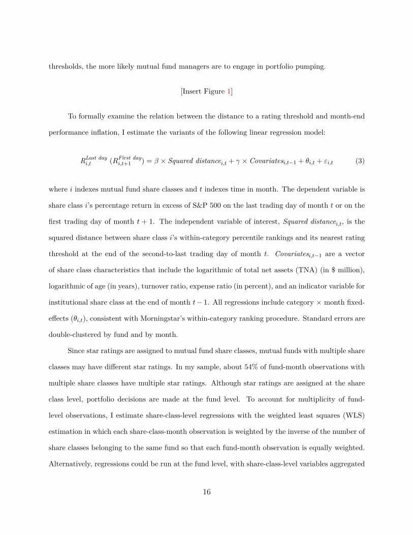
To formally examine the relation between the distance to a rating threshold and month-end

performance inflation, I estimate the variants of the following linear regression model:

RLast dayi,t (RFirst day

i,t+1 ) = β × Squared distancei,t + γ × Covariatesi,t−1 + θi,t + εi,t (3)

where i indexes mutual fund share classes and t indexes time in month. The dependent variable is

share class i’s percentage return in excess of S&P 500 on the last trading day of month t or on the

first trading day of month t + 1. The independent variable of interest, Squared distancei,t, is the

squared distance between share class i’s within-category percentile rankings and its nearest rating

threshold at the end of the second-to-last trading day of month t. Covariatesi,t−1 are a vector

of share class characteristics that include the logarithmic of total net assets (TNA) (in $ million),

logarithmic of age (in years), turnover ratio, expense ratio (in percent), and an indicator variable for

institutional share class at the end of month t− 1. All regressions include category × month fixed-

effects (θi,t), consistent with Morningstar’s within-category ranking procedure. Standard errors are

double-clustered by fund and by month.

Since star ratings are assigned to mutual fund share classes, mutual funds with multiple share

classes may have different star ratings. In my sample, about 54% of fund-month observations with

multiple share classes have multiple star ratings. Although star ratings are assigned at the share

class level, portfolio decisions are made at the fund level. To account for multiplicity of fund-

level observations, I estimate share-class-level regressions with the weighted least squares (WLS)

estimation in which each share-class-month observation is weighted by the inverse of the number of

share classes belonging to the same fund so that each fund-month observation is equally weighted.

Alternatively, regressions could be run at the fund level, with share-class-level variables aggregated

16

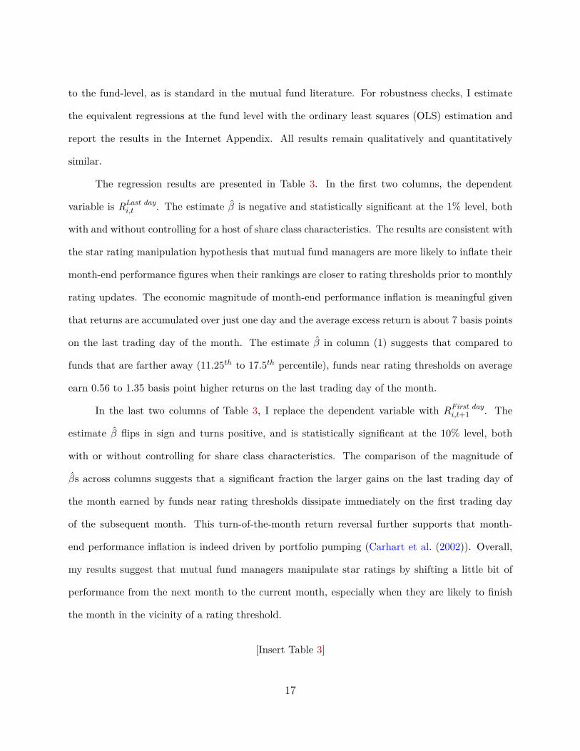
to the fund-level, as is standard in the mutual fund literature. For robustness checks, I estimate

the equivalent regressions at the fund level with the ordinary least squares (OLS) estimation and

report the results in the Internet Appendix. All results remain qualitatively and quantitatively

similar.

The regression results are presented in Table 3. In the first two columns, the dependent

variable is RLast dayi,t . The estimate β̂ is negative and statistically significant at the 1% level, both

with and without controlling for a host of share class characteristics. The results are consistent with

the star rating manipulation hypothesis that mutual fund managers are more likely to inflate their

month-end performance figures when their rankings are closer to rating thresholds prior to monthly

rating updates. The economic magnitude of month-end performance inflation is meaningful given

that returns are accumulated over just one day and the average excess return is about 7 basis points

on the last trading day of the month. The estimate β̂ in column (1) suggests that compared to

funds that are farther away (11.25th to 17.5th percentile), funds near rating thresholds on average

earn 0.56 to 1.35 basis point higher returns on the last trading day of the month.

In the last two columns of Table 3, I replace the dependent variable with RFirst dayi,t+1 . The

estimate β̂ flips in sign and turns positive, and is statistically significant at the 10% level, both

with or without controlling for share class characteristics. The comparison of the magnitude of

β̂s across columns suggests that a significant fraction the larger gains on the last trading day of

the month earned by funds near rating thresholds dissipate immediately on the first trading day

of the subsequent month. This turn-of-the-month return reversal further supports that month-

end performance inflation is indeed driven by portfolio pumping (Carhart et al. (2002)). Overall,

my results suggest that mutual fund managers manipulate star ratings by shifting a little bit of

performance from the next month to the current month, especially when they are likely to finish

the month in the vicinity of a rating threshold.

[Insert Table 3]

17

5.2 Placebo Tests

Some may concern that higher returns on the last trading day of the month earned by funds

near rating thresholds could be driven by other factors that are also correlated with the distance

to a rating threshold prior to rating updates. To address potential endogeneity concerns, I conduct

placebo tests to corroborate that the month-end performance inflation that I document in the

previous subsection is indeed specifically designed to inflate star ratings.

5.2.1 Reversing the June 2002 Morningstar’s Star Rating Methodology

To establish causality, I exploit the June 2002 change in Morningstar’s star rating method-

ology (e.g., Evans and Sun (Forthcoming)). In addition to changing the risk adjustment process,

Morningstar refined its peer groups used to rank mutual funds. In June 2002, Morningstar started

raking U.S. equity mutual funds within its nine (three-by-three style box) categories along the size

dimension (small, mid-cap, or large) and value dimension (value, blend, or growth), whereas all

U.S. equity mutual funds were ranked against each other within a single category group prior to

the change.

I measure placebo within-category percentile rankings by reversing the June 2002 change in

Morningstar’s star rating methodology. That is, I rank U.S. equity mutual funds within Morn-

ingstar’s nine categories on the basis of the new version of MRAR (Morningstar (2016)) until May

2002, while ranking all U.S. equity mutual funds against each other within a single category group

on the basis of the old version of MRAR (Blume (1998)) starting in June 2002. Then, I compute the

placebo distance to a rating threshold as the distance between placebo within-category percentile

rankings and the nearest rating threshold.

Not surprisingly, placebo within-category percentile rankings are highly correlated with the

ones that closely follow Morningstar’s star rating methodology (correlation coefficient = 0.76),

as shown in Panel A of Figure 2. Nevertheless, using a slightly different ranking methodology

18

has a significant impact on within-category percentile rankings when measured relative to rating

thresholds. Put differently, a small distortion of within-category percentile rankings results in a

large change in distances to rating thresholds. As shown in Panel B of Figure 2, the correlation

between placebo distances to rating thresholds and the ones that are based on Morningstar’s star

rating methodology is very low (correlation coefficient = 0.10).

[Insert Figure 2]

Using the placebo distance to a rating threshold, I estimate the variants of the following linear

regression model:


i,t+1 ) = β × Squared placebo distancei,t + γ × Covariatesi,t−1 + θi,t + εi,t (4)


share class i’s percentage return in excess of S&P 500 on the last trading day of month t or on the

first trading day of month t+ 1. Squared placebo distancei,t is the squared distance between share

class i’s placebo within-category percentile rankings and its nearest rating threshold at the end of the

second-to-last trading day of month t. Covariatesi,t−1 are the same set of share class characteristics

as in Equation (3). All regressions include category × month fixed-effects (θi,t), consistent with

Morningstar’s within-category ranking procedure, and are estimated with the weighted least squares

(WLS) estimation in which each share-class-month observation is weighted by the inverse of the

number of share classes belonging to the same fund. Standard errors are double-clustered by fund

and by month.


variable is RLast dayi,t . The estimate β̂ is close to zero and statistically insignificant, with or without

controls for share class characteristics. In addition, the estimate β̂ is positive, rather than being

negative. In the last two columns, I replace the dependent variable with RFirst dayi,t+1 . Again, the

19

estimate β̂ is close to zero and statistically insignificant. Thus, the placebo distance to a rating

threshold does not have any discernible impact on month-end performance inflation. The null

results in placebo tests corroborate that the month-end performance inflation that I document in

Section 5.1 is indeed specifically designed to influence star ratings. Furthermore, the null effects

from a slight distortion of within-category percentile rankings from the ones that closely follow

Morningstar’s star rating methodology also support the implicit identifying assumption that mutual

fund managers have fairly precise knowledge about their rankings prior to monthly rating updates.

[Insert Table 4]

5.2.2 Using Index Funds

Unlike actively-managed mutual funds, index mutual funds that are passively tracking bench-

mark indexes have limited incentives and abilities to pump their portfolios. For this reason, index

funds have thus far been excluded from the analysis, although they are kept in the ranking pro-

cedure to be consistent with Morningstar’s star rating methodology. I conduct additional placebo

tests using index mutual funds. Specifically, I re-estimate the linear regression model in Equation

(3) using a sample of index funds.


variable is RLast dayi,t . The estimate β̂ is close to zero and statistically insignificant, with or without

controls for share class characteristics. In addition, the estimate β̂ is positive, rather than being

negative. In the last two columns, I replace the dependent variable with RFirst dayi,t+1 . Again, the

estimate β̂ is close to zero and statistically insignificant. Thus, my results suggest that there is no

relation between the distance to a rating threshold and month-end performance inflation among

index funds. The null results in a sample of index funds further mitigate potential endogeneity

concerns that higher returns on the last trading day of the month earned by funds near rating

thresholds could be driven by other factors that are also correlated with the distance to a rating

20

threshold prior to rating updates.

[Insert Table 5]

5.3 Are All Star Ratings Created Equal?

Star rating manipulation has unique cross-sectional predictions about the extent to which

fund managers manipulate star ratings because not all star ratings are created equal. Building on

this observation, I test a set of cross-sectional predictions that star rating manipulation through

month-end performance inflation should be more pronounced among mutual funds with greater

incentives and abilities to manipulate star ratings.

First, since the assignment of star ratings is subject to data availability, it becomes much

more difficult for funds to manipulate star ratings as their return history extends further. While

completely determining overall star ratings for mutual fund share classes with a return history

of less than five years, three-year star ratings based on the past 36 monthly returns account for

only a small faction (20 to 40 percent) of overall star ratings for mutual fund share classes with

a longer return history. Second, Reuter and Zitzewitz (2015) find that discontinuities in the flow-

performance relation are greater at higher rating cutoffs and strongest at the four/five-star cutoff.

Similarly, Del Guercio and Tkac (2008) find that among all rating changes, upgrades from four

to five stars have the greatest impact on fund flows. Hence, the negative relation between the

distance to a rating threshold and month-end performance inflation should be more pronounced

among funds with a return history of less than five years and around the four/five-star cutoff.

To test the above cross-sectional predictions, I add an interaction term in Equation (3) and

estimate the variants of the following linear regression model:

RLast dayi,t = δ × Squared distancei,t × Sensitivityi,t

+ β × Squared distancei,t + ρ× Sensitivityi,t + γ × Covariatesi,t−1 + θi,t + εi,t

(5)

21

where i indexes mutual fund share classes and t indexes time in month. The dependent vari-

able is share class i’s percentage return in excess of S&P 500 on the last trading day of month

t. Squared distancei,t is the squared distance between share class i’s within-category percentile

rankings and its nearest rating threshold at the end of the second-to-last trading day of month t.

The interaction term, Sensitivityi,t, is (1) an indicator variable that takes the value of one if share

class i’s overall star ratings at the end of month t are to be completely determined by three-year

star ratings and zero otherwise, or (2) an indicator variable that takes the value of one if share

class i’s within-category percentile rankings are closest to the four/five-star cutoff at the end of

the second-to-last trading day of month t and zero otherwise. Covariatesi,t−1 are the same set of

share class characteristics as in Equation (3). All regressions include category × month fixed-effects

(θi,t), consistent with Morningstar’s within-category ranking procedure, and are estimated with the

weighted least squares (WLS) estimation in which each share-class-month observation is weighted

by the inverse of the number of share classes belonging to the same fund. Standard errors are


The regression results are presented in Table 6. In the first two columns, Sensitivityi,t is

an indicator variable for three-year star ratings. Consistent with my prediction, the estimate δ̂ is

negative and statistically significant at the 5% level. In addition, the estimate β̂ is also negative

and statistically significant at the conventional levels, and the magnitude of δ̂ is about two to three

times as large as that of β̂. Compared to young funds that are farther away (11.25th to 17.5th

percentile), young funds with a return history of less than five years that are near rating thresholds

on average earn 1.0 to 2.5 basis point higher returns on the last trading day of the month. This

negative relation is weaker among older funds with a return history of at least five years.

[Insert Table 6]

In the last two columns of Table 6, Sensitivityi,t is an indicator variable for four/five-star

cutoff. Consistent with my prediction, the estimate δ̂ is negative and statistically significant at the

22

5% level. In addition, the estimate β̂ is also negative and statistically significant at the 5% level

without controls in column (3), although it loses its statistical significance (t-statistic = −1.55) with

controls for share class characteristics in column (4). The magnitude of δ̂ is about five to six times

as large as that of β̂. Overall, my results suggest that star rating manipulation through portfolio

pumping is much more pronounced among funds around the four/five-star cutoff, consistent with

the star rating effect on fund flows (Del Guercio and Tkac (2008), Reuter and Zitzewitz (2015)).

In the corresponding fund-level regression results presented in Table IA5 in the Internet

Appendix, an indicator variable is replaced by the proportion of a fund’s total net assets belonging

to its share classes for which an indicator variable takes the value of one. Consistent with the

share-class-level WLS results, the fund-level OLS results show that the negative relation between

the distance to a rating threshold and month-end performance inflation is more pronounced among

funds for which a greater fraction of their total net assets consist of share classes with a return

history of less than five years and share classes around the four/five-star cutoff.

5.4 More Cross-sectional Tests

Prior studies on portfolio pumping make several cross-sectional predictions about the extent

to which fund managers engage in portfolio pumping. Building on the prior literature, I test a

set of cross-sectional predictions that portfolio pumping to manipulate star ratings should be more

pronounced among funds with greater incentives and abilities to pump their portfolios.

First, Carhart et al. (2002) argue that if fund managers are indeed “marking up” their

portfolio values, performance inflation should be more pronounced among small-cap funds because

the closing prices of less liquid stocks would presumably be easier to influence. Second, Patel

and Sarkissian (Forthcoming) argue that peer effects among teams such as the presence of peer

monitoring and joint monetary incentives are effective in deterring fund managers from engaging

in illegal trading activities such as portfolio pumping. Hence, the negative relation between the

23

distance to a rating threshold and month-end performance inflation should be more pronounced

among small-cap funds and single-managed funds, weakening as the size of management team

increases.

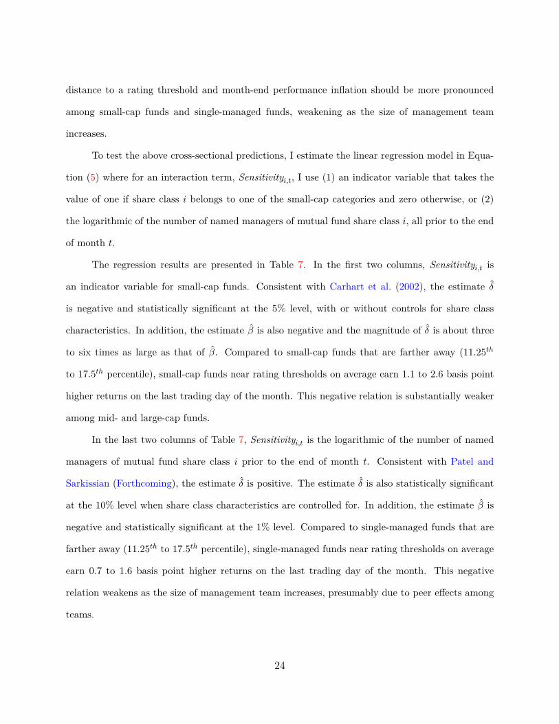
To test the above cross-sectional predictions, I estimate the linear regression model in Equa-

tion (5) where for an interaction term, Sensitivityi,t, I use (1) an indicator variable that takes the

value of one if share class i belongs to one of the small-cap categories and zero otherwise, or (2)

the logarithmic of the number of named managers of mutual fund share class i, all prior to the end

of month t.

The regression results are presented in Table 7. In the first two columns, Sensitivityi,t is

an indicator variable for small-cap funds. Consistent with Carhart et al. (2002), the estimate δ̂

is negative and statistically significant at the 5% level, with or without controls for share class

characteristics. In addition, the estimate β̂ is also negative and the magnitude of δ̂ is about three

to six times as large as that of β̂. Compared to small-cap funds that are farther away (11.25th

to 17.5th percentile), small-cap funds near rating thresholds on average earn 1.1 to 2.6 basis point

higher returns on the last trading day of the month. This negative relation is substantially weaker

among mid- and large-cap funds.

In the last two columns of Table 7, Sensitivityi,t is the logarithmic of the number of named

managers of mutual fund share class i prior to the end of month t. Consistent with Patel and

Sarkissian (Forthcoming), the estimate δ̂ is positive. The estimate δ̂ is also statistically significant

at the 10% level when share class characteristics are controlled for. In addition, the estimate β̂ is

negative and statistically significant at the 1% level. Compared to single-managed funds that are

farther away (11.25th to 17.5th percentile), single-managed funds near rating thresholds on average

earn 0.7 to 1.6 basis point higher returns on the last trading day of the month. This negative

relation weakens as the size of management team increases, presumably due to peer effects among

teams.

24

[Insert Table 7]

5.5 Has Portfolio Pumping Become More Evasive?

After the initial results of Carhart et al. (2002) drew a great deal of attention from regula-

tors, academics, and practitioners, the U.S. Securities and Exchange Commission (SEC) began to

investigate suspicious trading activities such as portfolio pumping (Duong and Meschke (2020)).

Consistent with heightened regulatory attention, recent studies find that portfolio pumping has

become more evasive (e.g., Hu et al. (2014), Wang (2019)). My results are also consistent with the

notion that fund managers exercise caution when they engage in illegal trading activities such as

portfolio pumping. Specifically, the extent to which fund managers inflate their month-end perfor-

mance figures is greater when fund rankings are closer to the rating thresholds prior to monthly

rating updates.

I conjecture that fund managers may pump their portfolios to manipulate star ratings when

portfolio pumping is less likely to attract regulatory attention. Just like academic studies on

portfolio pumping that have largely focused on quarter-ends (especially year-ends), the regulatory

attention may also have been limited to quarter/year-ends that are naturally more important

because reporting on a quarterly, semi-annual, or annual basis is common in the mutual fund

industry. Duong and Meschke (2020) find that compared to the early period of 1992 to 2000,

portfolio pumping has substantially declined at quarter-ends and almost disappeared at year-ends

in the later period of 2001 to 2011. These findings are not inconsistent with my conjecture. Unlike

prior studies, my paper focuses on all month-ends, allowing me to directly test the above conjecture

that portfolio pumping may have migrated from quarter/year-ends to less prominent month-ends.

To test the above conjecture, I add an interaction term in Equation (3) and estimate the

25

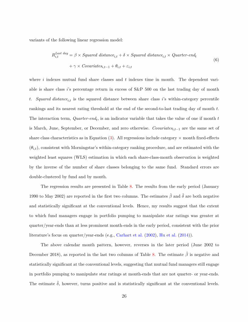
variants of the following linear regression model:

RLast dayi,t = β × Squared distancei,t + δ × Squared distancei,t ×Quarter-endt

+ γ × Covariatesi,t−1 + θi,t + εi,t

(6)

where i indexes mutual fund share classes and t indexes time in month. The dependent vari-

able is share class i’s percentage return in excess of S&P 500 on the last trading day of month

t. Squared distancei,t is the squared distance between share class i’s within-category percentile

rankings and its nearest rating threshold at the end of the second-to-last trading day of month t.

The interaction term, Quarter-endt, is an indicator variable that takes the value of one if month t

is March, June, September, or December, and zero otherwise. Covariatesi,t−1 are the same set of


(θi,t), consistent with Morningstar’s within-category ranking procedure, and are estimated with the

weighted least squares (WLS) estimation in which each share-class-month observation is weighted

by the inverse of the number of share classes belonging to the same fund. Standard errors are


The regression results are presented in Table 8. The results from the early period (January

1990 to May 2002) are reported in the first two columns. The estimates β̂ and δ̂ are both negative

and statistically significant at the conventional levels. Hence, my results suggest that the extent

to which fund managers engage in portfolio pumping to manipulate star ratings was greater at

quarter/year-ends than at less prominent month-ends in the early period, consistent with the prior

literature’s focus on quarter/year-ends (e.g., Carhart et al. (2002), Hu et al. (2014)).

The above calendar month pattern, however, reverses in the later period (June 2002 to

December 2018), as reported in the last two columns of Table 8. The estimate β̂ is negative and

statistically significant at the conventional levels, suggesting that mutual fund managers still engage

in portfolio pumping to manipulate star ratings at month-ends that are not quarter- or year-ends.

The estimate δ̂, however, turns positive and is statistically significant at the conventional levels.

26

The sum of the estimates (β̂ + δ̂) is close to zero and statistically insignificant. Thus, portfolio

pumping to manipulate star ratings has largely disappeared at quarter/year-ends, consistent with

Duong and Meschke (2020).

Overall, my results in this subsection suggest that following heightened regulatory scrutiny

prompted by Carhart et al. (2002), portfolio pumping to manipulate star ratings appears to have

largely migrated from quarter/year-ends to less prominent month-ends. This calendar effect, which

is novel to the literature on portfolio pumping, is consistent with the findings in recent studies that

portfolio pumping has become more evasive (e.g., Hu et al. (2014), Wang (2019)).

[Insert Table 8]

5.6 Robustness Checks

In this subsection, I provide some robustness checks on my baseline results in Section 5.1.

For the main identification, I exploit cross-sectional variation in the distance to a rating threshold

prior to monthly rating updates. Alternatively, I could exploit time-series variation in percentile

rankings and distances to rating thresholds because star ratings are based on the past performance

on a rolling basis. For instance, a fund’s rankings may sharply rise (or fall) as the fund “rolls”

out of a bad month and “rolls” into a good month (or vice versa). Building on this observation,

I exploit time-series variation in the distance to a rating threshold to explain the month-end

performance inflation. Specifically, I replace category × month fixed-effects with fund fixed-effects

and re-estimate the linear regression model in Equation (3). As reported in Panel A of Table 9,

my results remain qualitatively similar. Funds tend to earn higher returns on the last trading day

of the month when their rankings are closer to rating thresholds, compared to when their rankings

are farther away from rating thresholds.

In Section 5.1, I use the squared distance to a rating threshold as the independent variable

of interest to reflect the curvature in the relation between the distance to a rating threshold and

27

month-end performance inflation, as shown in Figure 1. For a robustness check, I replace the

squared distance with the distance and re-estimate the linear regression model in Equation (3). As

reported in Panel B of Table 9, my results remain qualitatively similar. Compared to distant peers,

mutual funds near rating thresholds tend to earn significantly higher returns on the last trading

day of the month, which partially reverses on the first trading day of the next month.

[Insert Table 9]

6 The Effects of Star Rating Manipulation

Some may wonder what fund managers would gain from engaging in portfolio pumping be-

cause it only shifts a little bit of performance from the next month to the current month. In this

section, I exploit the two-stage least squares (2SLS) estimation to show that portfolio pumping can

temporarily inflate star ratings, thereby increasing future fund flows, especially in the month of a

rating upgrade.

6.1 The Effect of Portfolio Pumping on Star Ratings

The results in Section 5 suggest that fund managers manipulate star ratings by inflating

month-end portfolio values, especially when their funds are likely to finish the month near rating

cutoffs. Portfolio pumping, however, could lower performance figures for the next month because

because a large fraction of gains on the last trading day of the month dissipate immediately on the

first trading day of the subsequent month. Theoretical studies on portfolio pumping also suggest

that portfolio pumping, while improving a fund’s short-term values, may hurt its long-term values

(e.g., Bhattacharyya and Nanda (2013)). In this subsection, I examine the net effect of portfolio

pumping on star ratings in the current and subsequent months as a first-step to examining the effects

of star rating manipulation. To account for the adverse effect of portfolio pumping on performance

figures for the next month, I use the turn-of-the-month return reversal, RLast dayi,t −RFirst day

i,t+12 , instead

28

of the return on the last day of the month, to measure the extent to which fund managers engage

in portfolio pumping.

Specifically, I estimate the variants of the following linear regression model:

1(Ratings changei,t+s) = β×RLast dayi,t −RFirst day

i,t+12 +γ×Covariatesi,t−1+θi,t+s+εi,t+s, s = 0, 1 (7)


(1) 1(Upgradet), which is an indicator variable that takes the value of one if share class i receives a

rating upgrade at the end of month t and zero otherwise, or (2) 1(Downgradet+1 | Upgradet), which

is an indicator variable that takes the value of one if share class i receives a rating downgrade at

the end of month t+ 1 after receiving a rating upgrade at the end of month t and zero otherwise.

The independent variable of interest, (RLast dayi,t − RFirst day

i,t+1 )/2, is share class i’s return reversal

around the turn of month t. Returns are in excess of S&P 500. Covariatesi,t−1 are the same set of


(θi,t+s) to be consistent with Morningstar’s within-category ranking procedure, and are estimated

with the weighted least squares (WLS) estimation in which each share-class-month observation is

weighted by the inverse of the number of share classes belonging to the same fund. Standard errors

are double-clustered by fund and by month.

The regression results are presented in Table 10. In columns (1) and (2), the dependent

variable is 1(Upgradet). In column (1), the estimate β̂ is positive and statistically significant at the

1% level, suggesting that portfolio pumping is effective in inflating star ratings at the end of the

month. The estimate β̂ remains largely unchanged when share class characteristics are controlled

for in column (2). One standard deviation increase in the return reversal around the turn of the

month is associated with a 77 basis point increase in the probability of a rating upgrade at the end

of the month. The economic magnitude is also meaningful given that the unconditional probability

of a rating upgrade is about 7 percent.

29

In columns (3) and (4), I replace the dependent variable with 1(Downgradei,t+1 | Upgradei,t).

The estimate β̂ is positive and statistically significant at the 1% level, suggesting that portfolio

pumping also increases the conditional probability of an immediate rating downgrade at the end of

the subsequent month following a rating upgrade. One standard deviation increase in the return

reversal around the turn of the month is associated with a 2.97 percent increase in the probability of

an immediate rating downgrade following an upgrade. The economic magnitude is also meaningful

given that the conditional probability of an immediate rating downgrade following an upgrade is

about 29 percent.

Overall, the results suggest that portfolio pumping is effective in inflating star ratings. Those

inflated star ratings induced by portfolio pumping are more likely to revert back to the previous

level in the subsequent month. These results are consistent with prior studies suggesting that

portfolio pumping is effective only in the short run (e.g., Bhattacharyya and Nanda (2013)). Next,

I turn to examining how portfolio pumping affects future fund flows by temporarily inflating star

ratings.

[Insert Table 10]

6.2 The Effect of Star Rating Manipulation on Fund Flows

Examining the effect of star rating manipulation on fund flows poses an empirical challenge

because changes in star ratings (especially upgrades) have a large impact on fund flows (Del Guercio

and Tkac (2008)) and a rating upgrade is at most only partially attributable to portfolio pumping.

To tease out the effect of a rating upgrade that can be attributable to portfolio pumping, I exploit

the following two-stage least squares (2SLS) estimation: In the first stage, I estimate the effect

of portfolio pumping on a rating upgrade as a linear probability model, as in Section 6.1. In the

second stage, I estimate the effect of star rating manipulation on fund flows using the fitted value

of the probability of a rating upgrade from the first-stage regression.

30

Specifically, I estimate the variants of the following 2SLS model:

1(Upgradei,t) = β1 ×RLast dayi,t −RFirst day

i,t+12 + γ1 × Covariatesi,t−1

+ η1 ×Additional controlsi,t + θ1,i,t + ε1,i,t (first stage)(8)

Flowi,t+s = β2 × ̂1(Upgradei,t) + γ2 × Covariatesi,t−1

+ η1 ×Additional controlsi,t + θ2,i,t+s + ε2,i,t+s, s = 1, 2, 3 (second stage)(9)

where i indexes mutual fund share classes and t indexes time in month. The first-stage regression

in Equation (8) is similar to that in Equation (7) in the previous subsection. In the second-stage,

the dependent variable, Flowi,t+s, is share class i’ fund flows as percentage of the beginning-of-the-

month TNA during month t + s, s = 1, 2, 3. The independent variable of interest, ̂1(Upgradei,t),

is the fitted value of the probability of a rating upgrade at the end of month t from the corre-

sponding first-stage regression. Covariatesi,t−1 include the same set of share class characteristics as

in Equation (3). Additional controlsi,t include contemporaneous and lagged fund flows (Flowi,t−s)

and returns (Ri,t−s), s = 0, 1, 2. The contemporaneous return, Rex Last Dayi,t , is cumulative only up

to the second-to-last trading day of month t. Returns are in excess of S&P 500. All regressions

include category × month fixed-effects (θ1,i,t, θ2,i,t+s) to be consistent with Morningstar’s within-

category ranking procedure, and are estimated with the weighted least squares (WLS) estimation in

which each share-class-month observation is weighted by the inverse of the number of share classes

belonging to the same fund. Standard errors are double-clustered by fund and by month.

The 2SLS results are presented in Table 11. The first-stage regression in columns (1) and

(2) is similar to the one in column (2) of Table 10, except for Additional controlsi,t including con-

temporaneous fund flows and returns in column (1) and contemporaneous and lagged fund flows

and returns in column (2). Consistent with the results in the previous subsection, the estimate

β̂1 is positive and statistically significant at the 1% level, suggesting that portfolio pumping sig-

nificantly increases the probability of a rating upgrade at the end of the month. The inclusion

31

of contemporaneous and lagged returns and flows only strengthens the results. Not surprisingly,

the contemporaneous return up to the second-to-last trading day of the month also significantly

increases the probability of a rating upgrade at the end of the month. In contrast, lagged returns do

not have any significant impact on a rating upgrade at the end of the month because these returns

affect star ratings both at the end of month t and month t− 1. That is, changes in star ratings are

primarily driven by the exclusion of the oldest month’s return and inclusion of the current month’s

return on a rolling basis in the computation of Morningstar Risk-Adjusted Returns (MRAR).

In the second-stage regression in columns (3) and (4), the dependent variable is Flowi,t+1.

In column (3), the estimate β̂2 is positive and statistically significant at the 1% level, suggesting

that star rating manipulation leads to additional fund flows in the month of a rating upgrade. The

estimate β̂2 remains qualitatively and quantitatively similar when I additionally control for lagged

fund flows and returns in column (4). In the remaining columns, I replace the dependent variable

with Flowi,t+s, s = 2, 3. The estimate β̂2 is positive, albeit statistically insignificant, suggesting

that portfolio pumping does not lower fund flows in the subsequent months. If anything, the gains

in fund flows extend beyond the month of a rating upgrade.

Overall, the 2SLS results suggest that portfolio pumping increases the probability of a rating

update at the end of the month (first-stage), thereby increasing fund flows, especially in the month

of a rating upgrade (second-stage). As inflated star ratings revert to the previous level in the

subsequent month, fund flows also tend to subside to the previous level in the following months.

Nevertheless, the gains in fund flows driven by star rating manipulation through portfolio pumping

are not offset by any significant reductions in fund flows in the subsequent months.

[Insert Table 11]

32

7 Conclusion

The idea that mutual fund investors use risk-adjusted returns in their capital allocation

decision is appealing and has motivated some prominent financial economists to use mutual fund

flows to test asset pricing models. Berk and van Binsbergen (2016), for instance, conclude that

the capital asset pricing model (CAPM) is the “closest to the asset pricing model investors are

actually using.” Barber et al. (2016) independently reach the same conclusion. Evans and Sun

(Forthcoming), however, argue that mutual fund investors actually follow simple heuristics such as

star ratings that are strongly correlated with the CAPM alpha. Ben-David et al. (2019) further

argue that star ratings explain mutual fund investors’ behavior much better than any asset pricing

models, concluding that star ratings are the main determinant of capital allocation across mutual

funds.

Given that mutual fund investors rely heavily on star ratings, it is natural to ask whether

and how star ratings distort the incentives of mutual fund managers. The incentive to inflate

performance metrics is naturally greater when funds are closer to rating cutoffs because even a

small increase in fund rankings (such as going from 89th percentile to 90th percentile) can make

discrete changes in star ratings (such as going from four stars to five stars) and lead to a large

jump in fund flows (Reuter and Zitzewitz (2015)). Consistent with this prediction, I find that U.S.

equity mutual fund managers manipulate star ratings by inflating month-end portfolio values when

they are likely to finish the month in the vicinity of rating thresholds.

Compared to their distant peers, mutual funds near rating thresholds experience substantially

larger gains on the last trading day of the month, which partially dissipate on the next trading

day. These results suggest that the closer fund rankings are to rating cutoffs, the greater the extent

to which portfolio managers engage in portfolio pumping (Zweig (1997), Carhart et al. (2002)).

Placebo tests exploiting the June 2002 change in Morningstar’s rating methodology yield expected

null effects, corroborating that month-end performance inflation is indeed specifically designed to

33

inflate star ratings. In cross-sectional tests, I further show that portfolio pumping to manipulate

star ratings is more pronounced among funds with greater incentives and abilities to pump their

portfolios and manipulate star ratings. For instance, star rating manipulation through portfolio

pumping is more pronounced among funds with a shorter return history and around the four/five

star rating cutoff. Exploiting the two-stage least squares (2SLS) estimation, I show that portfolio

pumping increases the probability of a rating update at the end of the month, thereby increasing

future fund flows, especially in the month of a rating upgrade.

34

References

Barber, Brad M., Xing Huang, and Terrance Odean, 2016, Which factors matter to investors?

Evidence from mutual fund flows, Review of Financial Studies 29, 2600–2642.

Begley, Taylor A., 2015, The real costs of corporate credit ratings, Working Paper .

Ben-David, Itzhak, Francesco Franzoni, Augustin Landier, and Rabih Moussawi, 2013, Do hedge

funds manipulate stock prices?, Journal of Finance 68, 2383–2434.

Ben-David, Itzhak, Jiacui Li, Andrea Rossi, and Yang Song, 2019, What do mutual fund investors

really care about?, Working Paper .

Berk, Jonathan B., and Jules H. van Binsbergen, 2016, Assessing asset pricing models using revealed

preference, Journal of Financial Economics 119, 1–23.

Bhattacharyya, Sugato, and Vikram Nanda, 2013, Portfolio pumping, trading activity and fund

performance, Review of Finance 17, 885–919.

Blume, Marshall E., 1998, An anatomy of Morningstar ratings, Financial Analysts Journal 54,

19–27.

Bollen, Nicolas P.B., and Veronika K. Pool, 2009, Do hedge fund managers misreport returns?

Evidence from the pooled distribution, Journal of Finance 64, 2257–2288.

Carhart, Mark M, 1997, On persistence in mutual fund performance, Journal of Finance 52, 57–82.

Carhart, Mark M., Ron Kaniel, David K. Musto, and Adam V. Reed, 2002, Leaning for the tape:

Evidence of gaming behavior in equity mutual funds, Journal of Finance 57, 661–693.

Chevalier, Judith, and Glenn Ellison, 1997, Risk taking by mutual funds as a response to incentives,

Journal of Political Economy 105, 1167–1200.

35

Daniel, Kent, Mark Grinblatt, Sheridan Titman, and Russ Wermers, 1997, Measuring mutual fund

performance with characteristic-based benchmarks, Journal of Finance 52, 1035–1058.

Del Guercio, Diane, and Paula A Tkac, 2008, Star power: The effect of Morningstar ratings on

mutual fund flow, Journal of Financial and Quantitative Analysis 43, 907–936.

Duong, Truong X., and Felix Meschke, 2020, The rise and fall of portfolio pumping among U.S.

mutual funds, Journal of Corporate Finance 60.

Evans, Richard B, and Yang Sun, Forthcoming, Models or stars: The role of asset pricing models

and heuristics in investor risk adjustment, Review of Financial Studies .

Fama, Eugene F, and James MacBeth, 1973, Risk, return, and equilibrium: Empirical tests, Journal

of Political Economy 81, 607–636.

Hu, Gang, R David Mclean, Jeffrey Pontiff, and Qinghai Wang, 2014, The year-end trading ac-

tivities of institutional investors: Evidence from daily trades, Review of Financial Studies 27,

1593–1614.

Ippolito, Richard A., 1992, Consumer reaction to measures of poor quality: Evidence from the

mutual fund industry, Journal of Law and Economics 35, 45–70.

Jensen, Michael C ., 1969, Risk, the pricing of capital assets, and the evaluation of investment

portfolios, Journal of Business 42, 167–247.

Lee, Jung Hoon, Charles Trzcinka, and Shyam Venkatesan, 2019, Do portfolio manager contracts

contract portfolio management?, Journal of Finance 74, 2543–2577.

Morningstar, 2016, Morningstar Rating for Funds .

Patel, Saurin, and Sergei Sarkissian, Forthcoming, Portfolio pumping and managerial structure,

Review of Financial Studies .

36

Reuter, Jonathan, and Eric Zitzewitz, 2015, How much does size erode mutual fund performance?

A regression discontinuity approach, Working Paper .

Sharpe, William F, 1998, Morningstar’s risk-adjusted ratings, Financial Analysts Journal 54, 21–33.

Sirri, Erik R, and Peter Tufano, 1998, Costly search and mutual fund flows, Journal of Finance 53,

1589–1622.

Wang, Pingle, 2019, Portfolio pumping in mutual fund families, Working Paper .

Zweig, Jason, 1997, Watch out for the year-end fund flimflam, Money Magazine November 1,

130–133.

37

Panel A: On the last day of month t Panel B: On the first day of month t+ 1

Figure 1: Distance to a Rating Threshold and Month-End NAV Inflation

This figure plots the average fund returns in excess of the S&P 500 index on the last trading day of month tin Panel A and on the first trading day of month t+ 1 in Panel B across equally spaced bins of the distanceto a rating threshold at the end of the second-to-last trading day of month t. For each bin with the equallength of one-tenth of a percentile (i.e., 0.001), I compute average daily returns of mutual fund share classesin excess of the S&P 500 index across each cross-section, weighted by the inverse of the number of shareclasses belonging to the same fund. Then, I compute the time-series averages of the cross-sectional averageexcess returns in the spirit of Fama and MacBeth (1973). In addition, I estimate the fitted curve from theregression of the excess return on the squared distance to a rating threshold and report a 95% confidenceinterval in the shaded area. The sample covers the period from 1990 to 2018.

38

Panel A: Within-category percentile rankings Panel B: Distances to rating thresholds

Figure 2: Correlation between Actual vs. Placebo Rankings and Distances to RatingThresholds

This figure shows the correlation between actual within-category percentile rankings and placebo within-category percentile rankings (correlation coefficient = 0.76) in Panel A and the correlation between actualdistances to rating thresholds and placebo distances to rating thresholds (correlation coefficient = 0.10) inPanel B. Actual within-category percentile rankings and distances to rating thresholds are based on theactual Morningstar rating methodology. Placebo within-category percentile rankings and distances to ratingthresholds are obtained by reversing the June 2002 change in Morningstar rating methodology. That is, Icompute placebo within-category percentile rankings using the new rating methodology until May 2002 andthe old one starting in June 2002. Then, I compute the placebo distance to a rating threshold as the distancebetween placebo within-category percentile rankings and the nearest rating threshold. The details on theconstruction of distance measures are provided in Section 4.

39

Table 1: Transition Matrix of Star Ratings

This table reports the transition matrix where each element in row i and column j represents the probability(in percent) of a mutual fund share class receiving star rating j at the end of month t conditional on itsreceiving star rating i at the end of month t − 1. At the end of each month, mutual fund share classes arerated by Morningstar on an integer scale of one star (the lowest rating) to five stars (the highest rating) onthe basis of Morningstar Risk-Adjusted Return (MRAR) over the prior three, five, and ten years, dependingon data availability. On the basis of within-category rankings of MRAR, the top 10% of mutual fund shareclasses receive five stars, the next 22.5% four stars, the middle 35% three stars, the next 22.5% two stars,and the bottom 10% receive one star. Overall star ratings are determined by the weighted averages of three,five, and ten-year star ratings, depending on data availability, rounded to the nearest integer value. Shareclasses less than three years old are not rated. Share classes at least three years old but less than five yearsold are rated based only on three-year star ratings. Share classes at least five years old but less than tenyears old are rated based on three-year star ratings (40 percent weight) and five-year star ratings (60 percentweight). Share classes at least ten years old are rated based on three-year star ratings (20 percent weight),five-year star ratings (30 percent weight), and ten-year star ratings (50 percent weight).

Panel A: Three-year star ratingsAt the end of month t

At the end of month t− 1 ? ?? ? ? ? ? ? ?? ? ? ? ? ?

? 87.08 12.63 0.24 0.04 0.01?? 5.20 83.82 10.82 0.15 0.01

? ? ? 0.05 8.21 84.10 7.54 0.10? ? ?? 0.02 0.15 13.16 80.75 5.92

? ? ? ? ? 0.004 0.04 0.38 14.93 84.65

Panel B: Five-year star ratingsAt the end of month t


? 89.50 10.33 0.13 0.03 0.01?? 4.39 86.69 8.80 0.10 0.02

? ? ? 0.03 6.73 87.18 6.00 0.06? ? ?? 0.01 0.09 10.78 84.28 4.84

? ? ? ? ? 0.003 0.01 0.21 12.30 87.47

40

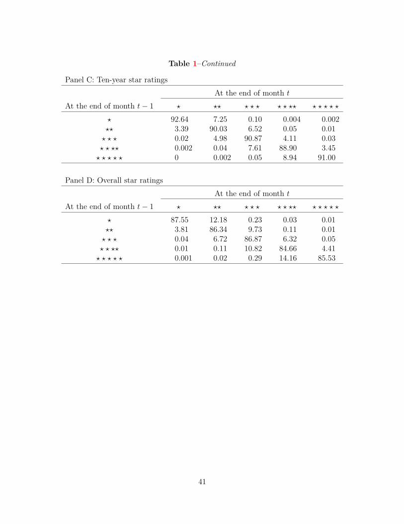
Table 1–Continued

Panel C: Ten-year star ratingsAt the end of month t


? 92.64 7.25 0.10 0.004 0.002?? 3.39 90.03 6.52 0.05 0.01

? ? ? 0.02 4.98 90.87 4.11 0.03? ? ?? 0.002 0.04 7.61 88.90 3.45

? ? ? ? ? 0 0.002 0.05 8.94 91.00

Panel D: Overall star ratingsAt the end of month t


? 87.55 12.18 0.23 0.03 0.01?? 3.81 86.34 9.73 0.11 0.01

? ? ? 0.04 6.72 86.87 6.32 0.05? ? ?? 0.01 0.11 10.82 84.66 4.41

? ? ? ? ? 0.001 0.02 0.29 14.16 85.53

41

Table 2: Summary Statistics

This table reports the summary statistics on the share-class-level variables.RLast Dayt and RFirst Day

t+1 are a mutual fund share class’s returns (in percent) on the last trading day of month tand on the first trading day of month t+1, respectively. Returns are in excess of the S&P 500 index. Distance,is the distance (in decimals) between a mutual fund share class’s within-category percentile rankings and itsnearest rating threshold at the end of the second-to-last trading day of the month. Placebo distance is thedistance (in decimals) between a mutual fund share class’s placebo within-category percentile rankings and itsnearest rating threshold at the end of the second-to-last trading day of the month. Placebo within-categorypercentile rankings are obtained by reversing the June 2002 change in Morningstar rating methodology.The details on the construction of distance measures are provided in Section 4. Share class characteristicsinclude total net assets (TNA) (in $ million), age (in years), turnover ratio, expense ratio (in percent), andan indicator variable for institutional share class. 1(Small-cap) is an indicator variable that takes the valueof one if a mutual fund share class belongs to one of the small-cap categories and zero otherwise. N Managersis the number of named managers of a mutual fund share class. 1(Three-year rating) is an indicator variablethat takes the value of one if a mutual fund share class’s overall star ratings at the end of the monthare to be completely determined by three-year star ratings and zero otherwise. 1(Four/five-star cutoff) isan indicator variable that takes the value of one if a mutual fund share class’s within-category percentilerankings are closest to the four/five-star cutoff at the end of the second-to-last trading day of the monthand zero otherwise. 1(Quarter-end) is an indicator variable that takes the value of one if a month is March,June, September, or December, and zero otherwise. 1(Upgradet) is an indicator variable that takes thevalue of one if a mutual fund share class receives a rating upgrade at the end of month t and zero otherwise.1(Downgradet+s | Upgradet) is an indicator variable that takes the value of one if a mutual fund share classreceives a rating downgrade at the end of month t+ s after receiving an upgrade at the end of month t andzero otherwise (s = 1, 2). Flowt+s is a mutual fund share class’s fund flows as percentage of the beginning-of-the-month TNA during month t + s (s = −2,−1, 0, 1, 2, 3). Rt+s is a mutual fund share class’s returnduring month t− s (s = 1, 2). Rex Last Day

t is a mutual fund share class’s return during month t cumulativeup to the second-to-last trading day of month t. All continuous variables are winsorized at 1% and 99%.The sample covers the period from 1990 to 2018.

Variable Obs. Mean St. Dev. Q1 Median Q3

RLast Dayt (%) 1, 252, 358 0.07 0.43 −0.14 0.05 0.26

RFirst Dayt+1 (%) 1, 252, 358 −0.03 0.47 −0.24 −0.01 0.21

(RLast Dayt −RFirst Day

t+1 )/2 (%) 1, 252, 358 0.05 0.33 −0.12 0.03 0.20Distance 1, 252, 358 0.07 0.05 0.03 0.06 0.10Placebo distance 1, 252, 358 0.07 0.04 0.03 0.06 0.10TNA (in $million) 1, 141, 114 467.33 1, 295.58 12.48 65.81 301.41Age (in years) 1, 252, 358 11.64 9.20 5.67 9.21 14.35Turnover 1, 218, 346 0.77 0.63 0.34 0.61 1.01Expense ratio (%) 1, 218, 613 1.33 0.49 0.98 1.25 1.651(Institutional) 1, 252, 358 0.19 0.40 0 0 01(Small-cap) 1, 252, 358 0.22 0.41 0 0 0N Managers 1, 239, 838 2.66 2.03 1 2 31(Three-year rating) 1, 252, 358 0.23 0.42 0 0 01(Four/five-star cutoff) 1, 252, 358 0.14 0.35 0 0 01(Quarter-end) 1, 252, 358 0.34 0.47 0 0 1

42

Table 2–Continued


1(Upgradet) 1, 241, 336 0.07 0.26 0.00 0.00 0.001(Downgradet+1 | Upgradet) 86, 391 0.29 0.45 0.00 0.00 1.001(Downgradet+2 | Upgradet) 85, 911 0.34 0.48 0.00 0.00 1.00Flowt−2 (%) 1, 122, 543 0.06 8.12 −1.78 −0.50 0.76Flowt−1 (%) 1, 122, 543 −0.04 7.68 −1.81 −0.51 0.74Flowt (%) 1, 126, 532 0.06 8.95 −1.81 −0.51 0.74Flowt+1 (%) 1, 120, 116 −0.03 8.06 −1.82 −0.52 0.72Flowt+2 (%) 1, 113, 624 −0.08 7.62 −1.82 −0.53 0.70Flowt+3(%) 1, 108, 185 −0.13 7.33 −1.83 −0.54 0.68Rt−2 (%) 1, 252, 358 0.13 2.12 −0.88 0.10 1.11Rt−1 (%) 1, 252, 358 0.13 2.11 −0.87 0.10 1.11Rex Last Dayt (%) 1, 252, 358 0.05 2.07 −0.91 0.05 1.03

43

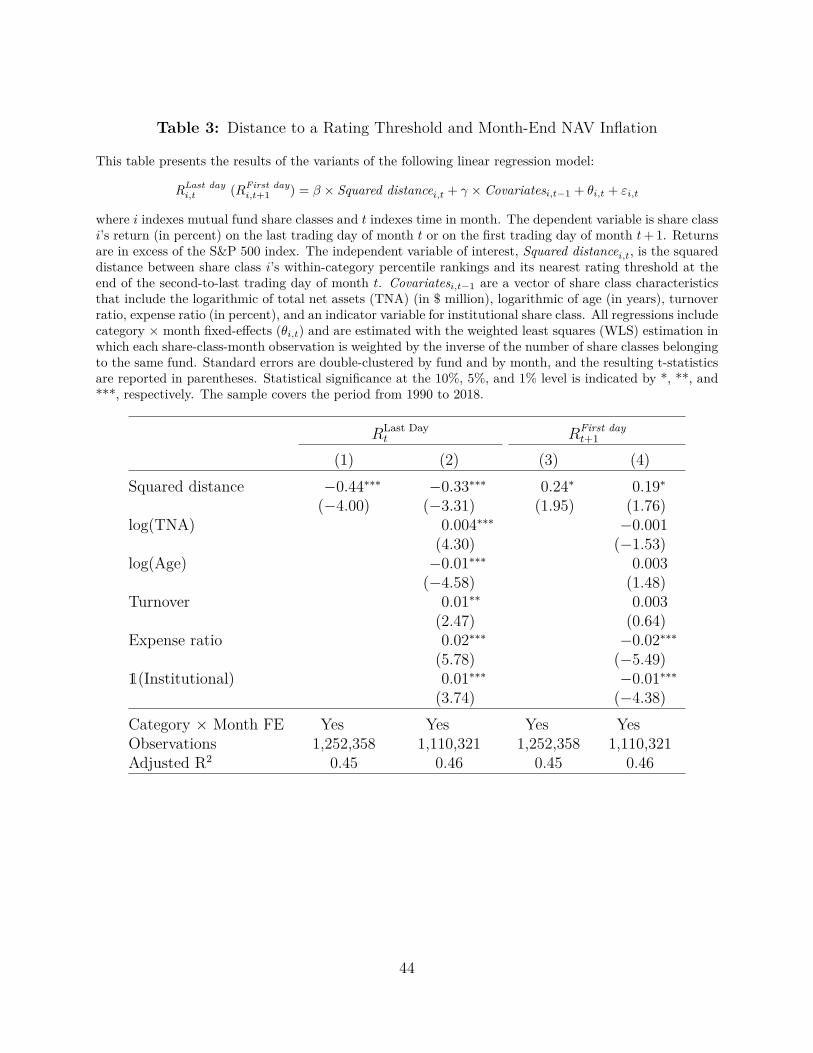
Table 3: Distance to a Rating Threshold and Month-End NAV Inflation

This table presents the results of the variants of the following linear regression model:


i,t+1 ) = β × Squared distancei,t + γ × Covariatesi,t−1 + θi,t + εi,t

where i indexes mutual fund share classes and t indexes time in month. The dependent variable is share classi’s return (in percent) on the last trading day of month t or on the first trading day of month t+ 1. Returnsare in excess of the S&P 500 index. The independent variable of interest, Squared distancei,t, is the squareddistance between share class i’s within-category percentile rankings and its nearest rating threshold at theend of the second-to-last trading day of month t. Covariatesi,t−1 are a vector of share class characteristicsthat include the logarithmic of total net assets (TNA) (in $ million), logarithmic of age (in years), turnoverratio, expense ratio (in percent), and an indicator variable for institutional share class. All regressions includecategory × month fixed-effects (θi,t) and are estimated with the weighted least squares (WLS) estimation inwhich each share-class-month observation is weighted by the inverse of the number of share classes belongingto the same fund. Standard errors are double-clustered by fund and by month, and the resulting t-statisticsare reported in parentheses. Statistical significance at the 10%, 5%, and 1% level is indicated by *, **, and***, respectively. The sample covers the period from 1990 to 2018.

RLast Dayt RFirst day

t+1

(1) (2) (3) (4)Squared distance −0.44∗∗∗ −0.33∗∗∗ 0.24∗ 0.19∗

(−4.00) (−3.31) (1.95) (1.76)log(TNA) 0.004∗∗∗ −0.001

(4.30) (−1.53)log(Age) −0.01∗∗∗ 0.003

(−4.58) (1.48)Turnover 0.01∗∗ 0.003

(2.47) (0.64)Expense ratio 0.02∗∗∗ −0.02∗∗∗

(5.78) (−5.49)1(Institutional) 0.01∗∗∗ −0.01∗∗∗

(3.74) (−4.38)Category × Month FE Yes Yes Yes YesObservations 1,252,358 1,110,321 1,252,358 1,110,321Adjusted R2 0.45 0.46 0.45 0.46

44

Table 4: Placebo Tests: Reversing the June 2002 Change in Morningstar Rating Method-ology



i,t+1 ) = β × Squared placebo distancei,t + γ × Covariatesi,t−1 + θi,t + εi,t

where i indexes mutual fund share classes and t indexes time in month. The dependent variable is shareclass i’s return (in percent) on the last trading day of month t or on the first trading day of month t + 1.Returns are in excess of the S&P 500 index. The independent variable of interest, Squared placebo distancei,t,is the squared distance between share class i’s placebo within-category percentile rankings and its nearestrating threshold at the end of the second-to-last trading day of month t. Placebo within-category percentilerankings are obtained by reversing the June 2002 change in Morningstar rating methodology. That is, Icompute placebo within-category percentile rankings using the new rating methodology until May 2002 andthe old one starting in June 2002. Covariatesi,t−1 are the same set of share class characteristics as in Table3. All regressions include category × month fixed-effects (θi,t) and are estimated with the weighted leastsquares (WLS) estimation in which each share-class-month observation is weighted by the inverse of thenumber of share classes belonging to the same fund. Standard errors are double-clustered by fund and bymonth, and the resulting t-statistics are reported in parentheses. Statistical significance at the 10%, 5%,and 1% level is indicated by *, **, and ***, respectively. The sample covers the period from 1990 to 2018.


t+1

(1) (2) (3) (4)Squared placebo distance 0.01 0.09 0.09 0.03

(0.13) (1.03) (1.10) (0.39)log(TNA) 0.004∗∗∗ −0.001

(4.14) (−1.47)log(Age) −0.01∗∗∗ 0.003

(−4.45) (1.47)Turnover 0.01∗∗ 0.004

(2.47) (0.68)Expense ratio 0.02∗∗∗ −0.02∗∗∗

(5.69) (−5.36)1(Institutional) 0.01∗∗∗ −0.01∗∗∗


45

Table 5: Placebo Tests: Index Funds

This table presents the results of the variants of the following linear regression model in a sample of indexfunds:


i,t+1 ) = β × Squared distancei,t + γ × Covariatesi,t−1 + θi,t + εi,t

where i indexes mutual fund share classes and t indexes time in month. The dependent variable is shareclass i’s return (in percent) on the last trading day of month t or on the first trading day of month t + 1.Returns are in excess of the S&P 500 index. The independent variable of interest, Squared distancei,t, is thesquared distance between share class i’s within-category percentile rankings and its nearest rating thresholdat the end of the second-to-last trading day of month t. Covariatesi,t−1 are the same set of share classcharacteristics as in Table 3. All regressions include category × month fixed-effects (θi,t) and are estimatedwith the weighted least squares (WLS) estimation in which each share-class-month observation is weighted bythe inverse of the number of share classes belonging to the same fund. Standard errors are double-clusteredby fund and by month, and the resulting t-statistics are reported in parentheses. Statistical significance atthe 10%, 5%, and 1% level is indicated by *, **, and ***, respectively. The sample covers the period from1990 to 2018.


t+1

(1) (2) (3) (4)Squared distance 0.01 0.01 −0.01 −0.04

(0.04) (0.05) (−0.04) (−0.20)log(TNA) −0.0003 0.001

(−0.25) (0.89)log(Age) −0.002 0.001

(−0.20) (0.23)Turnover 0.002 −0.003

(0.38) (−0.76)Expense ratio −0.01 0.003

(−1.11) (0.43)1(Institutional) −0.003 0.002

(−0.45) (0.42)Category × Month FE Yes Yes Yes YesObservations 81,728 75,156 81,728 75,156Adjusted R2 0.72 0.72 0.74 0.75

46

Table 6: Are All Star Ratings Created Equal?



+ β × Squared distancei,t + ρ× Sensitivityi,t + γ × Covariatesi,t−1 + θi,t + εi,t

where i indexes mutual fund share classes and t indexes time in month. The dependent variable is shareclass i’s return (in percent) on the last trading day of month t. Returns are in excess of the S&P 500 index.Squared distancei,t is the squared distance between share class i’s within-category percentile rankings andits nearest rating threshold at the end of the second-to-last trading day of month t. Sensitivityi,t is (1) anindicator variable that takes the value of one if share class i’s overall star ratings at the end of month t areto be completely determined by three-year star ratings and zero otherwise, or (2) an indicator variable thattakes the value of one if share class i’s within-category percentile rankings are closest to the four/five-starcutoff at the end of the second-to-last trading day of month t and zero otherwise. Covariatesi,t−1 are thesame set of share class characteristics as in Table 3. All regressions include category × month fixed-effects(θi,t) and are estimated with the weighted least squares (WLS) estimation in which each share-class-monthobservation is weighted by the inverse of the number of share classes belonging to the same fund. Standarderrors are double-clustered by fund and by month, and the resulting t-statistics are reported in parentheses.Statistical significance at the 10%, 5%, and 1% level is indicated by *, **, and ***, respectively. The samplecovers the period from 1990 to 2018.

RLast Dayt

(1) (2) (3) (4)Squared distance × 1(Three-year rating) −0.52∗∗ −0.55∗∗

(−2.21) (−2.36)Squared distance × 1(Four/five-star cutoff) −1.38∗∗ −1.10∗∗

(−2.48) (−1.98)Squared distance −0.29∗∗∗ −0.19∗∗ −0.26∗∗ −0.19

(−2.85) (−2.07) (−2.07) (−1.55)1(Three-year rating) 0.01∗∗ −0.004

(2.17) (−1.35)1(Four/five-star cutoff) 0.02∗∗ 0.02∗

(2.08) (1.79)log(TNA) 0.004∗∗∗ 0.003∗∗∗

(4.04) (3.82)log(Age) −0.01∗∗∗ −0.01∗∗∗

(−4.48) (−3.85)Turnover 0.01∗∗ 0.01∗∗

(2.46) (2.49)Expense ratio 0.02∗∗∗ 0.02∗∗∗

(5.58) (5.69)1(Institutional) 0.01∗∗∗ 0.01∗∗∗

(3.71) (3.80)Category × Month FE Yes Yes Yes YesObservations 1,252,358 1,095,824 1,252,358 1,095,824Adjusted R2 0.45 0.46 0.45 0.46

47

Table 7: More Cross-Sectional Tests



+ β × Squared distancei,t + ρ× Sensitivityi,t + γ × Covariatesi,t−1 + θi,t (θt) + εi,t

where i indexes mutual fund share classes and t indexes time in month. The dependent variable is shareclass i’s return (in percent) on the last trading day of month t. Returns are in excess of the S&P 500 index.Squared distancei,t is the squared distance between share class i’s within-category percentile rankings andits nearest rating threshold at the end of the second-to-last trading day of month t. Sensitivityi,t is (1) anindicator variable that takes the value of one if share class i belongs to one of the small-cap categories andzero otherwise, or (2) the logarithmic of the number of named managers of mutual fund share class i, priorto the end of month t. Covariatesi,t−1 are the same set of share class characteristics as in Table 3. Allregressions include category × month fixed-effects (θi,t) or month fixed-effects (θt) and are estimated withthe weighted least squares (WLS) estimation in which each share-class-month observation is weighted by theinverse of the number of share classes belonging to the same fund. Standard errors are double-clustered byfund and by month, and the resulting t-statistics are reported in parentheses. Statistical significance at the10%, 5%, and 1% level is indicated by *, **, and ***, respectively. The sample covers the period from 1990to 2018.

RLast Dayt

(1) (2) (3) (4)Squared distance × 1(Small-cap) −0.63∗∗ −0.68∗∗

(−2.16) (−2.35)Squared distance × log(N Managers) 0.16 0.16∗

(1.62) (1.68)Squared distance −0.22∗ −0.12 −0.52∗∗∗ −0.44∗∗∗

(−1.85) (−1.11) (−3.55) (−3.31)1(Small-cap) 0.09∗∗∗ 0.08∗∗∗

(3.82) (3.61)log(N Managers) −0.0004 −0.001

(−0.24) (−0.30)log(TNA) 0.004∗∗∗ 0.004∗∗∗

(4.18) (4.24)log(Age) −0.01∗∗∗ −0.01∗∗∗

(−3.77) (−4.40)Turnover 0.01∗∗ 0.01∗∗

(2.21) (2.36)Expense ratio 0.02∗∗∗ 0.02∗∗∗

(5.38) (5.59)1(Institutional) 0.01∗∗∗ 0.01∗∗∗

(2.79) (3.61)Category × Month FE No No Yes YesMonth FE Yes Yes No NoObservations 1,252,358 1,095,824 1,239,838 1,085,804Adjusted R2 0.29 0.30 0.46 0.47

48

Table 8: Has Portfolio Pumping Become More Evasive?

This table presents the results of the variants of the following linear regression model in sub-periods:

RLast dayi,t = β × Squared distancei,t + δ × Squared distancei,t ×Quarter-endt + γ × Covariatesi,t−1 + θi,t + εi,t

where i indexes mutual fund share classes and t indexes time in month. The dependent variable is shareclass i’s return (in percent) on the last trading day of month t. Returns are in excess of the S&P 500 index.Squared distancei,t is the squared distance between share class i’s within-category percentile rankings and itsnearest rating threshold at the end of the second-to-last trading day of month t. Quarter-endt is an indicatorvariable that takes the value of one if month t is March, June, September, or December, and zero otherwise.Covariatesi,t−1 are the same set of share class characteristics as in Table 3. All regressions include category× month fixed-effects (θi,t) and are estimated with the weighted least squares (WLS) estimation in whicheach share-class-month observation is weighted by the inverse of the number of share classes belonging tothe same fund. Standard errors are double-clustered by fund and by month, and the resulting t-statisticsare reported in parentheses. Statistical significance at the 10%, 5%, and 1% level is indicated by *, **, and***, respectively. The sample covers the period from 1990 to 2018 and is split around the June 2002 changein Morningstar rating methodology.

RLast Dayt

1990:01–2002:05 2002:06–2018:12(1) (2) (3) (4)

Squared distance × 1(Quarter-end) −1.34∗ −1.51∗∗ 0.22∗ 0.24∗∗

(−1.79) (−2.05) (1.93) (2.08)Squared distance −1.11∗∗ −0.70∗ −0.17∗∗ −0.14∗

(−2.35) (−1.70) (−2.07) (−1.86)log(TNA) 0.004 0.002∗∗∗

(1.18) (4.32)log(Age) −0.01∗∗∗ −0.002

(−3.14) (−1.12)Turnover 0.04∗∗∗ 0.002

(2.64) (0.57)Expense ratio 0.06∗∗∗ 0.01∗∗∗

(4.86) (3.23)1(Institutional) 0.04∗∗∗ 0.002

(3.76) (1.00)Category × Month FE Yes Yes Yes YesObservations 160,944 151,052 1,091,414 944,772Adjusted R2 0.28 0.28 0.56 0.57

49

Table 9: Portfolio Pumping Induced by Star Ratings: Robustness Checks

This table presents the results of the variants of the following linear regression models:


i,t+1 ) = β × Squred distancei,t + γ × Covariatesi,t−1 + αi + εi,t

andRLast dayi,t (RFirst day

i,t+1 ) = β ×Distancei,t + γ × Covariatesi,t−1 + θi,t + εi,t

where i indexes mutual fund share classes and t indexes time in month. The dependent variable is shareclass i’s return (in percent) on the last trading day of month t or on the first trading day of month t + 1.Returns are in excess of the S&P 500 index. Squared distancei,t is the squared distance between share class i’swithin-category percentile rankings and its nearest rating threshold at the end of the second-to-last tradingday of month t. Covariatesi,t−1 are the same set of share class characteristics as in Table 3. All regressionsinclude fund fixed-effects (αi) or category × month fixed-effects (θi,t), and are estimated with the weightedleast squares (WLS) estimation in which each share-class-month observation is weighted by the inverse ofthe number of share classes belonging to the same fund. Standard errors are double-clustered by fund andtime, and the resulting t-statistics are reported in parentheses. Statistical significance at the 10%, 5%, and1% level is indicated by *, **, and ***, respectively. The sample covers the period from 1990 to 2018.

Panel A: Fund fixed-effects, instead of category × month fixed-effects


t+1

(1) (2) (3) (4)Squared distance −0.32∗∗∗ −0.19∗ 0.11 0.05

(−2.60) (−1.73) (0.83) (0.41)log(TNA) 0.01∗∗∗ −0.01∗∗

(3.17) (−2.09)log(Age) −0.06∗∗∗ 0.03∗

(−4.70) (1.85)Turnover 0.02∗∗ −0.003

(2.10) (−0.36)Expense ratio 0.003 −0.004

(0.45) (−0.73)Fund FE Yes Yes Yes YesObservations 1,252,358 1,095,824 1,252,358 1,095,824Adjusted R2 0.03 0.03 0.01 0.01

50

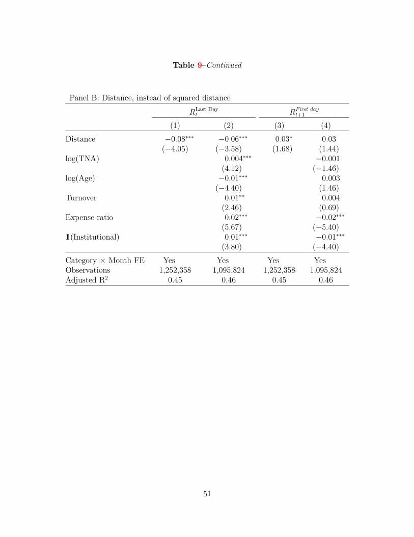
Table 9–Continued

Panel B: Distance, instead of squared distance


t+1

(1) (2) (3) (4)Distance −0.08∗∗∗ −0.06∗∗∗ 0.03∗ 0.03

(−4.05) (−3.58) (1.68) (1.44)log(TNA) 0.004∗∗∗ −0.001

(4.12) (−1.46)log(Age) −0.01∗∗∗ 0.003

(−4.40) (1.46)Turnover 0.01∗∗ 0.004

(2.46) (0.69)Expense ratio 0.02∗∗∗ −0.02∗∗∗

(5.67) (−5.40)1(Institutional) 0.01∗∗∗ −0.01∗∗∗


51

Table 10: The Effect of Portfolio Pumping on Star Ratings


1(Ratings changei,t+s) = β ×RLast Dayt −RFirst Day

t+12 + γ × Covariatesi,t−1 + θi,t+s + εi,t+s, s = 0, 1

where i indexes mutual fund share classes and t indexes time in month. The dependent variable is (1)1(Upgradei,t), which is an indicator variable that takes the value of one if share class i receives an upgradein star ratings at the end of month t and zero otherwise, or (2) 1(Downgradei,t+1 | Upgradei,t), which isan indicator variable that takes the value of one if share class i receives a downgrade in star ratings at theend of month t + 1 after receiving an upgrade at the end of month t and zero otherwise. The independentvariable of interest, (RLast day

i,t −RFirst dayi,t+1 )/2, is share class i’s daily return reversal (in percent) around the

turn of month t. Returns are in excess of the S&P 500 index. Covariatesi,t−1 are the same set of shareclass characteristics as in Table 3. All regressions include category × month fixed-effects (θi,t+s) and areestimated with the weighted least squares (WLS) estimation in which each share-class-month observationis weighted by the inverse of the number of share classes belonging to the same fund. Standard errors aredouble-clustered by fund and time, and the resulting t-statistics are reported in parentheses. Statisticalsignificance at the 10%, 5%, and 1% level is indicated by *, **, and ***, respectively. The sample covers theperiod from 1990 to 2018.

Dependent variable: 1(Upgradet) 1(Downgradet+1 | Upgradet)(1) (2) (3) (4)

(RLast Dayt −RFirst Day

t+1 )/2 0.02∗∗∗ 0.02∗∗∗ 0.09∗∗∗ 0.08∗∗∗

(3.74) (3.63) (6.25) (6.08)log(TNA) −0.001∗∗∗ 0.003∗∗∗

(−2.74) (2.66)log(Age) −0.01∗∗∗ 0.01∗

(−15.33) (1.96)Turnover 0.004∗∗∗ 0.002

(3.73) (0.60)Expense ratio 0.01∗∗∗ 0.01

(4.06) (1.63)1(Institutional) 0.002∗ −0.0002

(1.77) (−0.03)Category × Month FE Yes Yes Yes YesObservations 1,241,336 1,087,734 86,391 75,597Adjusted R2 0.01 0.01 0.06 0.06

52

Table 11: The Effect of Star Rating Manipulation on Fund Flows

This table presents the results of the variants of the following two-stage least squares (2SLS) model:

1(Upgradei,t) = β1 ×RLast Dayt −RFirst Day

t+12 + γ1 × Covariatesi,t−1 + η1 ×Additional controlsi,t + θ1,i,t + ε1,i,t (first stage)

Flowi,t+s = β2 × ̂1(Upgradei,t+1) + γ2 × Covariatesi,t−1 + η1 ×Additional controlsi,t + θ2,i,t+s + ε2,i,t+s, s = 1, 2, 3 (second stage)

where i indexes mutual fund share classes and t indexes time in month. In the first stage, the dependent variable is an indicator variablethat takes the value of one if share class i receives a rating upgrade at the end of month t and zero otherwise. The independent variable ofinterest in the first stage is share class i’s daily return reversal (in percent) around the turn of month t. Returns are in excess of the S&P500 index. In the second stage, the dependent variable is share class i’ fund flows as percentage of the beginning-of-the-month TNA duringmonth t+ s, s = 1, 2, 3. The independent variable of interest in the second stage is the fitted value of the dependent variable in the first stage.Covariatesi,t−1 are the same set of share class characteristics as in Table 3. Additional controlsi,t include contemporaneous and lagged fundflows (Flowi,t−s), lagged returns (Ri,t−s), s = 1, 2, and contemporaneous returns (Rex Last Day

t ) cumulative up to the second-to-last tradingday of month t. All regressions include category × month fixed-effects (θ) and are estimated with the weighted least squares (WLS) estimationin which each share-class-month observation is weighted by the inverse of the number of share classes belonging to the same fund. Standarderrors are double-clustered by fund and time, and the resulting t-statistics are reported in parentheses. Statistical significance at the 10%,5%, and 1% level is indicated by *, **, and ***, respectively. The sample covers the period from 1990 to 2018.53

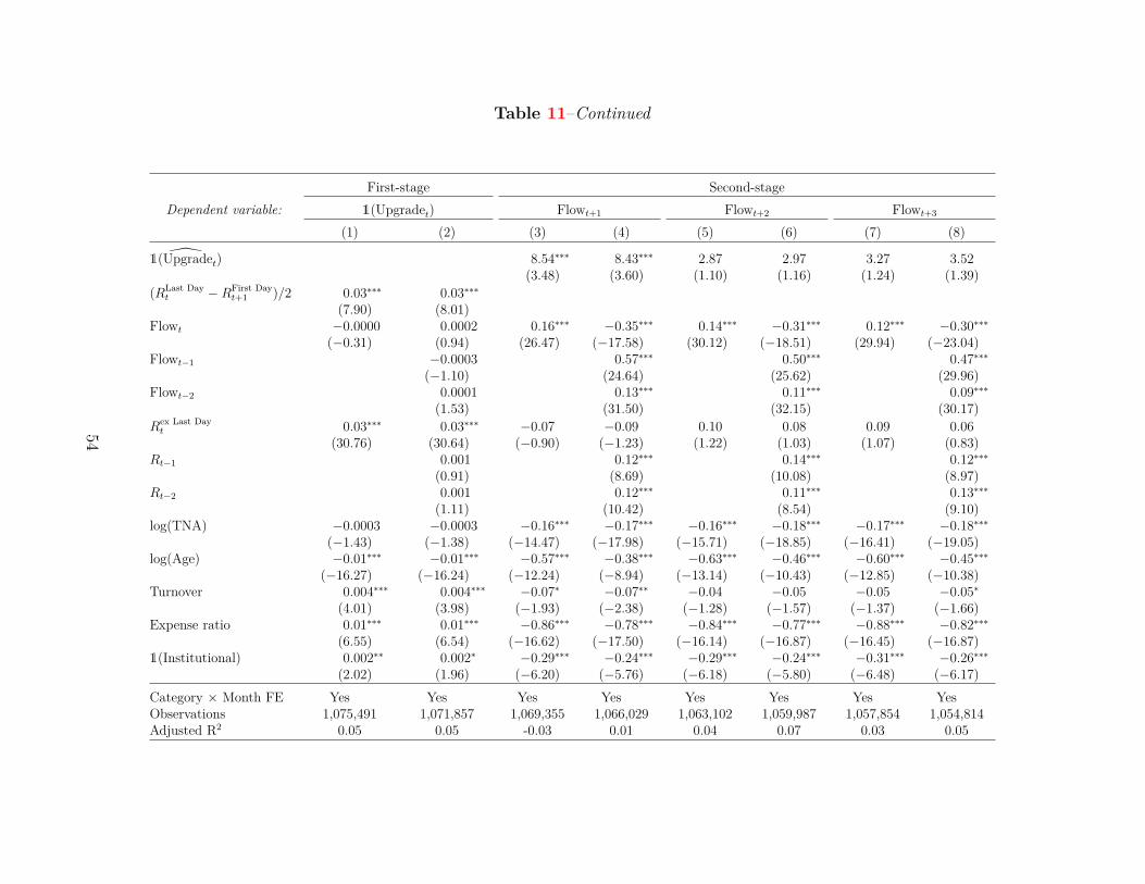
Table 11–Continued

First-stage Second-stageDependent variable: 1(Upgradet) Flowt+1 Flowt+2 Flowt+3

(1) (2) (3) (4) (5) (6) (7) (8)̂1(Upgradet) 8.54∗∗∗ 8.43∗∗∗ 2.87 2.97 3.27 3.52

(3.48) (3.60) (1.10) (1.16) (1.24) (1.39)(RLast Day

t −RFirst Dayt+1 )/2 0.03∗∗∗ 0.03∗∗∗

(7.90) (8.01)Flowt −0.0000 0.0002 0.16∗∗∗ −0.35∗∗∗ 0.14∗∗∗ −0.31∗∗∗ 0.12∗∗∗ −0.30∗∗∗

(−0.31) (0.94) (26.47) (−17.58) (30.12) (−18.51) (29.94) (−23.04)Flowt−1 −0.0003 0.57∗∗∗ 0.50∗∗∗ 0.47∗∗∗

(−1.10) (24.64) (25.62) (29.96)Flowt−2 0.0001 0.13∗∗∗ 0.11∗∗∗ 0.09∗∗∗

(1.53) (31.50) (32.15) (30.17)Rex Last Dayt 0.03∗∗∗ 0.03∗∗∗ −0.07 −0.09 0.10 0.08 0.09 0.06

(30.76) (30.64) (−0.90) (−1.23) (1.22) (1.03) (1.07) (0.83)Rt−1 0.001 0.12∗∗∗ 0.14∗∗∗ 0.12∗∗∗

(0.91) (8.69) (10.08) (8.97)Rt−2 0.001 0.12∗∗∗ 0.11∗∗∗ 0.13∗∗∗

(1.11) (10.42) (8.54) (9.10)log(TNA) −0.0003 −0.0003 −0.16∗∗∗ −0.17∗∗∗ −0.16∗∗∗ −0.18∗∗∗ −0.17∗∗∗ −0.18∗∗∗

(−1.43) (−1.38) (−14.47) (−17.98) (−15.71) (−18.85) (−16.41) (−19.05)log(Age) −0.01∗∗∗ −0.01∗∗∗ −0.57∗∗∗ −0.38∗∗∗ −0.63∗∗∗ −0.46∗∗∗ −0.60∗∗∗ −0.45∗∗∗

(−16.27) (−16.24) (−12.24) (−8.94) (−13.14) (−10.43) (−12.85) (−10.38)Turnover 0.004∗∗∗ 0.004∗∗∗ −0.07∗ −0.07∗∗ −0.04 −0.05 −0.05 −0.05∗

(4.01) (3.98) (−1.93) (−2.38) (−1.28) (−1.57) (−1.37) (−1.66)Expense ratio 0.01∗∗∗ 0.01∗∗∗ −0.86∗∗∗ −0.78∗∗∗ −0.84∗∗∗ −0.77∗∗∗ −0.88∗∗∗ −0.82∗∗∗

(6.55) (6.54) (−16.62) (−17.50) (−16.14) (−16.87) (−16.45) (−16.87)1(Institutional) 0.002∗∗ 0.002∗ −0.29∗∗∗ −0.24∗∗∗ −0.29∗∗∗ −0.24∗∗∗ −0.31∗∗∗ −0.26∗∗∗

(2.02) (1.96) (−6.20) (−5.76) (−6.18) (−5.80) (−6.48) (−6.17)Category × Month FE Yes Yes Yes Yes Yes Yes Yes YesObservations 1,075,491 1,071,857 1,069,355 1,066,029 1,063,102 1,059,987 1,057,854 1,054,814Adjusted R2 0.05 0.05 -0.03 0.01 0.04 0.07 0.03 0.05

54

Internet Appendix for

“Do Mutual Funds Manipulate Star Ratings?

Evidence from Portfolio Pumping”

Sanghyun (Hugh) Kim

This Internet Appendix provides fund-level results that are equivalent to the share-class-level results

presented in the main text. The fund-level results are obtained by aggregating share-class-level

variables to the fund-level and using the ordinary least squares (OLS) estimation.

Table IA1: Summary Statistics

This table reports the summary statistics on the fund-level variables.RLast Dayi,t and RFirst Day

i,t+1 are mutual fund i’s returns (in percent) on the last trading day of month t andon the first trading day of month t + 1, respectively. Returns are in excess of category benchmark returns,computed as average returns across mutual funds belonging to the same Morningstar category starting inJune 2002 and across all U.S. equity funds as a single category group prior to June 2002. Distancei,t, is thedistance (in decimals) between fund i’s within-category percentile rankings and its nearest rating thresholdat the end of the second-to-last trading day of month t. Placebo distancei,t is the distance (in decimals)between fund i’s placebo within-category percentile rankings and its nearest rating threshold at the endof the second-to-last trading day of month t. Placebo within-category percentile rankings are obtained byreversing the June 2002 change in Morningstar’s rating methodology when it refined its peer groups usedto rank mutual funds. The details on the construction of distance measures are provided in Section 4 ofthe main text. Fund characteristics include total net assets (TNA) (in $ million), age (in years), turnoverratio, and expense ratio (in percent). Month-end TNAi,t is deflated by 1 + RLast day

i,t to estimate its valueat the end of the second-to-last trading day of month t. For mutual funds with multiple share classes,share-class-level variables are aggregated to the fund level by computing the sum of TNAs, the maximum ofages, and the value-weighted averages for the rest of the share-class-level variables. % Institutional TNAi,t

is the proportion of TNAs from institutional share classes of mutual fund i. 1(Small-capi,t) is an indicatorvariable that takes the value of one if fund i belongs to one of the small-cap categories and zero otherwise.N Managersi,t is the number of named managers of mutual fund i. % Three-year TNAi,t is the proportionof TNAs from share classes of mutual fund i for which overall star ratings at the end of month t are tobe completely determined by three-year star ratings. 1(Four/five-star cutoffi,t) is an indicator variable thattakes the value of one if fund i’s within-category percentile rankings are closest to the four/five-star cutoffat the end of the second-to-last trading day of month t and zero otherwise. 1(Quarter-endt) is an indicatorvariable that takes the value of one if month t is March, June, September, or December, and zero otherwise.All continuous variables are winsorized at 1% and 99%. The sample covers the period from 1990 to 2018.


RLast Dayt (%) 466, 078 0.09 0.47 −0.14 0.06 0.30

RFirst Dayt+1 (%) 466, 078 −0.04 0.50 −0.26 −0.01 0.22

Distance 466, 078 0.07 0.04 0.03 0.06 0.10Placebo distance 466, 078 0.07 0.04 0.03 0.06 0.10TNA (in $million) 466, 078 1, 141.11 2, 839.99 68.70 253.21 941.11Age (in years) 466, 078 14.96 11.92 6.69 11.49 18.75Turnover 446, 445 0.76 0.65 0.32 0.59 1.00Expense ratio (%) 450, 524 1.17 0.41 0.92 1.13 1.39% Institutional TNA 466, 078 0.26 0.38 0 0 0.51(Small-cap) 466, 078 0.23 0.42 0 0 0N Managers 458, 059 2.51 2.02 1 2 3% Three-year rating TNA 466, 078 0.27 0.43 0 0 11(Four/five-star cutoff) 466, 078 0.17 0.36 0 0 01(Quarter-end) 466, 078 0.33 0.47 0 0 1

1

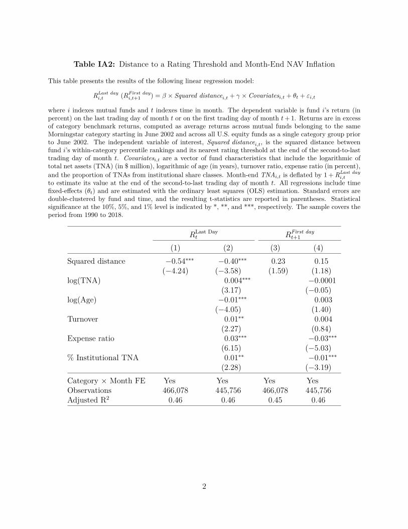
Table IA2: Distance to a Rating Threshold and Month-End NAV Inflation

This table presents the results of the following linear regression model:


i,t+1 ) = β × Squared distancei,t + γ × Covariatesi,t + θt + εi,t

where i indexes mutual funds and t indexes time in month. The dependent variable is fund i’s return (inpercent) on the last trading day of month t or on the first trading day of month t+ 1. Returns are in excessof category benchmark returns, computed as average returns across mutual funds belonging to the sameMorningstar category starting in June 2002 and across all U.S. equity funds as a single category group priorto June 2002. The independent variable of interest, Squared distancei,t, is the squared distance betweenfund i’s within-category percentile rankings and its nearest rating threshold at the end of the second-to-lasttrading day of month t. Covariatesi,t are a vector of fund characteristics that include the logarithmic oftotal net assets (TNA) (in $ million), logarithmic of age (in years), turnover ratio, expense ratio (in percent),and the proportion of TNAs from institutional share classes. Month-end TNAi,t is deflated by 1 + RLast day

i,t

to estimate its value at the end of the second-to-last trading day of month t. All regressions include timefixed-effects (θt) and are estimated with the ordinary least squares (OLS) estimation. Standard errors aredouble-clustered by fund and time, and the resulting t-statistics are reported in parentheses. Statisticalsignificance at the 10%, 5%, and 1% level is indicated by *, **, and ***, respectively. The sample covers theperiod from 1990 to 2018.


t+1

(1) (2) (3) (4)Squared distance −0.54∗∗∗ −0.40∗∗∗ 0.23 0.15

(−4.24) (−3.58) (1.59) (1.18)log(TNA) 0.004∗∗∗ −0.0001

(3.17) (−0.05)log(Age) −0.01∗∗∗ 0.003

(−4.05) (1.40)Turnover 0.01∗∗ 0.004

(2.27) (0.84)Expense ratio 0.03∗∗∗ −0.03∗∗∗

(6.15) (−5.03)% Institutional TNA 0.01∗∗ −0.01∗∗∗

(2.28) (−3.19)Category × Month FE Yes Yes Yes YesObservations 466,078 445,756 466,078 445,756Adjusted R2 0.46 0.46 0.45 0.46

2

Table IA3: Placebo Tests: Reversing the June 2002 Change in Morningstar’s RatingMethodology



i,t+1 ) = β × Squared placebo distancei,t + γ × Covariatesi,t + θt + εi,t

where i indexes mutual funds and t indexes time in month. The dependent variable is fund i’s return (inpercent) on the last trading day of month t or on the first trading day of month t + 1. Returns are inexcess of category benchmark returns, computed as average returns across mutual funds belonging to thesame Morningstar category starting in June 2002 and across all U.S. equity funds as a single category groupprior to June 2002. The independent variable of interest, Squared placebo distancei,t, is the squared distancebetween fund i’s placebo within-category percentile rankings and its nearest rating threshold at the endof the second-to-last trading day of month t. Placebo within-category percentile rankings are obtained byreversing the June 2002 change in Morningstar’s rating methodology when it refined its peer groups usedto rank mutual funds. To accomplish this, I rank mutual funds within Morningstar categories until May2002, while ranking all U.S. equity mutual funds against each other as a single category group starting inJune 2002. Covariatesi,t are the same set of fund characteristics as in Table IA2. All regressions includetime fixed-effects (θt) and are estimated with the ordinary least squares (OLS) estimation. Standard errorsare double-clustered by fund and time, and the resulting t-statistics are reported in parentheses. Statisticalsignificance at the 10%, 5%, and 1% level is indicated by *, **, and ***, respectively. The sample covers theperiod from 1990 to 2018.


t+1

(1) (2) (3) (4)Squared placebo distance −0.02 0.10 0.14 0.06

(−0.25) (1.01) (1.53) (0.69)log(TNA) 0.004∗∗∗ −0.0001

(3.20) (−0.06)log(Age) −0.01∗∗∗ 0.003

(−4.10) (1.40)Turnover 0.01∗∗ 0.004

(2.28) (0.84)Expense ratio 0.03∗∗∗ −0.03∗∗∗

(6.17) (−4.97)% Institutional TNA 0.01∗∗ −0.01∗∗∗

(2.27) (−3.19)Category × Month FE Yes Yes Yes YesObservations 466,078 445,756 466,078 445,756Adjusted R2 0.46 0.46 0.45 0.46

3

Table IA4: Placebo Tests: Index Funds

This table presents the results of the following linear regression model in a sample of index funds:


i,t+1 ) = β × Squared distancei,t + γ × Covariatesi,t + θt + εi,t

where i indexes mutual funds and t indexes time in month. The dependent variable is share class i’s return(in percent) on the last trading day of month t or on the first trading day of month t + 1. Returns are inexcess of category benchmark returns, computed as average returns across mutual funds belonging to thesame Morningstar category starting in June 2002 and across all U.S. equity funds as a single category groupprior to June 2002. Squared distancei,t is the squared distance between fund i’s within-category percentilerankings and its nearest rating threshold at the end of the second-to-last trading day of month t. Covariatesi,tare the same set of fund characteristics as in Table IA2. All regressions include time fixed-effects (θt) andare estimated with the ordinary least squares (OLS) estimation. Standard errors are double-clustered byfund and time, and the resulting t-statistics are reported in parentheses. Statistical significance at the 10%,5%, and 1% level is indicated by *, **, and ***, respectively. The sample covers the period from 1990 to2018.


t+1

(1) (2) (3) (4)Squared distance 0.003 0.03 −0.07 −0.09

(0.01) (0.15) (−0.29) (−0.36)log(TNA) −0.0003 0.002

(−0.16) (1.18)log(Age) 0.0001 −0.0001

(0.01) (−0.03)Turnover 0.001 −0.002

(0.12) (−0.54)Expense ratio −0.01 0.01

(−0.68) (0.61)% Institutional TNA −0.01 0.005

(−1.04) (0.86)Category × Month FE Yes Yes Yes YesObservations 36,077 34,999 36,077 34,999Adjusted R2 0.71 0.72 0.74 0.74

4

Table IA5: Are All Star Ratings Created Equal?



+ β × Squared distancei,t + ρ× Sensitivityi,t + γ × Covariatesi,t + θt + εi,t

where i indexes mutual funds and t indexes time in month. The dependent variable is fund i’s return (inpercent) on the last trading day of month t. Returns are in excess of category benchmark returns, computedas average returns across mutual funds belonging to the same Morningstar category starting in June 2002 andacross all U.S. equity funds as a single category group prior to June 2002. Squared distancei,t is the squareddistance between fund i’s within-category percentile rankings and its nearest rating threshold at the end ofthe second-to-last trading day of month t. Sensitivityi,t is (1) the proportion of TNAs from share classes ofmutual fund i for which overall star ratings at the end of month t are to be completely determined by three-year star ratings, or (2) an indicator variable that takes the value of one if fund i’s within-category percentilerankings are closest to the four/five-star cutoff at the end of the second-to-last trading day of month t andzero otherwise. Covariatesi,t are the same set of fund characteristics as in Table IA2. All regressions includetime fixed-effects (θt) and are estimated with the ordinary least squares (OLS) estimation. Standard errorsare double-clustered by fund and time, and the resulting t-statistics are reported in parentheses. Statisticalsignificance at the 10%, 5%, and 1% level is indicated by *, **, and ***, respectively. The sample covers theperiod from 1990 to 2018.

RLast Dayt

(1) (2) (3) (4)Squared distance × % Three-year rating TNA −0.71∗∗ −0.73∗∗∗

(−2.49) (−2.60)Squared distance × % Four/five-star cutoff TNA −1.53∗∗ −1.15∗

(−2.57) (−1.96)Squared distance −0.34∗∗∗ −0.21∗ −0.34∗∗ −0.23∗

(−2.87) (−1.94) (−2.33) (−1.66)% Three-year rating TNA 0.01∗∗ −0.005

(2.22) (−1.38)% Four/five-star cutoff TNA 0.02∗∗ 0.02∗

(2.05) (1.76)log(TNA) 0.004∗∗∗ 0.003∗∗∗

(3.15) (2.83)log(Age) −0.01∗∗∗ −0.01∗∗∗

(−4.24) (−3.50)Turnover 0.01∗∗ 0.01∗∗

(2.28) (2.32)Expense ratio 0.03∗∗∗ 0.03∗∗∗

(6.12) (6.15)% Institutional TNA 0.01∗∗ 0.01∗∗

(2.22) (2.34)Category × Month FE Yes Yes Yes YesObservations 466,078 445,756 466,078 445,756Adjusted R2 0.46 0.46 0.46 0.46

5

Table IA6: Cross-Section of Mutual Funds and the Star Rating Effect on Portfolio Pumping



+ β × Squared distancei,t + ρ× Sensitivityi,t + γ × Covariatesi,t + θt + εi,t

where i indexes mutual funds and t indexes time in month. The dependent variable is fund i’s return (inpercent) on the last trading day of month t. Returns are in excess of category benchmark returns, computedas average returns across mutual funds belonging to the same Morningstar category starting in June 2002and across all U.S. equity funds as a single category group prior to June 2002. Squared distancei,t is thesquared distance between fund i’s within-category percentile rankings and its nearest rating threshold at theend of the second-to-last trading day of month t. Sensitivityi,t is (1) an indicator variable that takes thevalue of one if fund i belongs to one of the small-cap categories and zero otherwise, or (2) the logarithmic ofthe number of named managers of mutual fund i, all prior to the end of month t. Covariatesi,t are the sameset of fund characteristics as in Table IA2. All regressions include time fixed-effects (θt) and are estimatedwith the ordinary least squares (OLS) estimation. Standard errors are double-clustered by fund and time,and the resulting t-statistics are reported in parentheses. Statistical significance at the 10%, 5%, and 1%level is indicated by *, **, and ***, respectively. The sample covers the period from 1990 to 2018.

RLast Dayt

(1) (2) (3) (4)Squared distance × 1(Small-cap) −0.46 −0.58∗

(−1.43) (−1.81)Squared distance × log(N Managers) 0.20∗ 0.21∗

(1.74) (1.89)Squared distance −0.33∗∗ −0.17 −0.66∗∗∗ −0.54∗∗∗

(−2.28) (−1.28) (−3.99) (−3.55)1(Small-cap) 0.08∗∗∗ 0.08∗∗∗

(3.75) (3.53)log(N Managers) −0.001 −0.0004

(−0.28) (−0.20)log(TNA) 0.004∗∗∗ 0.004∗∗∗

(3.29) (3.23)log(Age) −0.01∗∗∗ −0.01∗∗∗

(−3.43) (−4.05)Turnover 0.01∗∗ 0.01∗∗

(2.06) (2.18)Expense ratio 0.03∗∗∗ 0.03∗∗∗

(5.90) (6.04)% Institutional TNA 0.002 0.01∗∗

(0.69) (2.00)Category × Month FE No No Yes YesMonth FE Yes Yes No NoObservations 466,078 445,756 458,059 439,236Adjusted R2 0.30 0.30 0.46 0.46

6

Table IA7: The Fall of Portfolio Pumping? Quarter/Year-Ends vs. Other Month-Ends


RLast dayi,t = β × Squared distancei,t + δ × Squared distancei,t ×Quarter-endt + γ × Covariatesi,t + θt + εi,t

where i indexes mutual funds and t indexes time in month. The dependent variable is fund i’s return (inpercent) on the last trading day of month t. Returns are in excess of category benchmark returns, computedas average returns across mutual funds belonging to the same Morningstar category starting in June 2002and across all U.S. equity funds as a single category group prior to June 2002. Squared distancei,t is thesquared distance between fund i’s within-category percentile rankings and its nearest rating threshold at theend of the second-to-last trading day of month t. Quarter-endt is an indicator variable that takes the valueof one if month t is March, June, September, or December, and zero otherwise. Covariatesi,t are the sameset of fund characteristics as in Table IA2. All regressions include time fixed-effects (θt) and are estimatedwith the ordinary least squares (OLS) estimation. Standard errors are double-clustered by fund and time,and the resulting t-statistics are reported in parentheses. Statistical significance at the 10%, 5%, and 1%level is indicated by *, **, and ***, respectively. The sample covers the period from 1990 to 2018 and issplit around the June 2002 change in Morningstar’s rating methodology.

RLast Dayt

1990:01–2002:05 2002:06–2018:12(1) (2) (3) (4)

Squared distance × 1(Quarter-end) −1.51∗ −1.58∗∗ 0.31∗∗ 0.34∗∗

(−1.94) (−2.05) (2.07) (2.30)Squared distance −1.22∗∗ −0.75∗ −0.24∗∗ −0.20∗∗

(−2.43) (−1.71) (−2.36) (−2.11)log(TNA) 0.003 0.003∗∗∗

(0.90) (3.39)log(Age) −0.02∗∗∗ −0.001

(−3.57) (−0.83)Turnover 0.04∗∗ 0.002

(2.58) (0.48)Expense ratio 0.07∗∗∗ 0.01∗∗∗

(5.09) (3.99)% Institutional TNA 0.04∗∗∗ −0.002

(3.33) (−0.80)Time fixed-effects Yes Yes Yes YesObservations 110,665 104,657 355,413 341,099Adjusted R2 0.28 0.29 0.56 0.57

7

Do Mutual Funds Manipulate Star Ratings? Evidence from ...

Documents

Transcript of Do Mutual Funds Manipulate Star Ratings? Evidence from ...