Do Dividend Clienteles Exist? Evidence on

Dividend Preferences of Retail Investors∗

John Graham

Duke University

Fuqua School of Business

Alok Kumar

University of Notre Dame

Mendoza College of Business

December 12, 2003

(Comments are welcome)

∗Please address all correspondence to John Graham, Fuqua School of Business, Duke University, Box90120, Durham, NC 27708; Phone: 919-660-7857; email: john.graham@duke.edu OR Alok Kumar, 239Mendoza College of Business, University of Notre Dame, Notre Dame, IN 46556; Phone: 574-631-0354;email: akumar@nd.edu. We would like to thank Brad Barber, Robert Battalio, William Goetzmann, YanivGrinstein, Dong Hong, Sonya Lim, Roni Michaely, Paul Schultz, Hersh Shefrin, and Meir Statman for severalhelpful discussions and valuable comments. We thank Itamar Simonson for making the investor data availableto us and Terrance Odean for answering numerous questions about the investor database. All remainingerrors and omissions are our own.

Do Dividend Clienteles Exist? Evidence on

Dividend Preferences of Retail Investors

Abstract

We study the stock holdings and trading behavior of a representative group of more than

60,000 households and find evidence consistent with dividend clienteles. The stock holdings

of retail investors indicate a preference for dividend yield that increases with age (consistent

with life-cycle or consumption preferences) and decreases with income (consistent with low-

tax investors holding high-yield stocks) and risk aversion. The stock trading behavior of

retail investors provide reinforcing evidence of these dividend preferences. Older, low-income

investors disproportionally purchase stocks before the ex-dividend day. Among small stocks,

the ex-day premium increases with age and decreases with income, which is consistent with

tax explanations of the ex-day premium. We also find evidence that older, low-income

investors purchase stocks after they initiate dividends. Finally, we document that, consistent

with the attention hypothesis, older and low-income investors purchase stocks on and after

dividend announcement dates. These results have important policy implications because

they indicate that recent reductions in the dividend tax rate are not exclusively a “tax break

for the rich” because, in fact, the income streams of older and less wealthy investors benefit

more from the proposed policy changes.

Do individual (or retail) investors prefer dividends? If so, what are the main determinants

of their dividend preference? According to the traditional view (Miller and Modigliani 1961,

Elton and Gruber 1970), the difference in the dividend and capital gains tax rates influences

the dividend preference of investors. If there exists a positive differential between the tax

rates on dividends and capital gains, firms that pay higher dividends are likely to attract

groups of investors that have lower marginal tax rates. Low (high) income retail investors

face a negative (positive) dividend-capital gains tax rate differential. Hence, low (high)

income investors are likely to favor high (low) dividend yield stocks and consequently, a

tax-induced retail investor dividend clientele may emerge.

Some retail investors may exhibit a strong preference for dividend paying stocks in spite

of a tax disadvantage. For instance, investors with a high degree of risk aversion may prefer

a stream of relatively certain dividend payments over uncertain capital gains. Alternatively,

mental accounting (Thaler 1985) may influence investors’ dividend preference – investors who

keep dividend income and capital gains in two separate mental accounts may not treat them

equally. Such investors may prefer high dividend yield (DY) stocks because the dividend

income may act as a “silver-lining” when the capital gains are low or negative.

Life-cycle considerations may influence retail investors’ dividend preference too (Shefrin

and Thaler 1988). Older investors or any investor with a greater need for a regular in-

come stream may prefer high DY stocks if they use the dividend income to finance their

consumption. Due to self-control reasons, these investors may prefer cash dividends over

“home grown” dividends (i.e., income generated by the partial liquidation of the portfolio

or by holding relatively less risky bonds). Furthermore, to avoid regret, they may adopt

the heuristic “consume from dividend and keep the principal intact” (Shefrin and Statman

1984).

Taken together, mental accounting, regret and self-control based theories predict that

dividend income and capital gains need not be perfect substitutes and consumption from

dividends may be preferred over consumption from capital gains. In fact, Long (1978) pro-

vides evidence that suggests that the market is willing to pay a premium for cash dividends.

In addition to a “rational,” tax-induced clientele and a “behavioral,” age-based clientele,

other factors such as differential risk perceptions of investors and transaction costs may lead

to the formation of dividend clienteles. Investors may prefer to hold high DY stocks due to

their risk characteristics – high DY stocks are typically less risky than low DY stocks.

To summarize, there are several strong and theoretically sound reasons for the existence

of retail investor dividend clienteles. There is also a widespread belief that retail investors

1

prefer dividend income over capital gains and anecdotal as well as indirect evidence on the

existence of dividend clienteles from a variety of settings support such a belief (e.g., Elton

and Gruber (1970), Eades, Hess, and Kim (1984), Green and Rydqvist (1999)). The extant

evidence suggests that the dividend preference of retail investors is likely to be an important

determinant of firms’ payout policies. Brav, Graham, Harvey, and Michaely (2003) survey a

large number of CFOs, Treasurers and other managers to identify the main determinants of

firms’ payout policies. There is a strong belief among these financial executives that retail

investors’ prefer dividend paying stocks.1 Furthermore, several studies, either implicitly or

explicitly, assume the existence of a tax-based retail investor dividend clientele. However, so

far, direct evidence on the dividend preference of retail investors is scarce.

In this paper, using the investment accounts of more than 60,000 retail investors at a

large discount brokerage house in the U.S. during the 1991-96 time-period, we provide direct

evidence on the existence of retail investor dividend clienteles. We find that, as a group, retail

investors prefer non-dividend paying stocks over dividend paying stocks. However, within

the retail investor group, older and low-income investors prefer dividend paying stocks over

non-dividend paying stocks. Within the set of dividend paying stocks, as a group, retail

investors prefer high DY stocks over low DY stocks. Furthermore, older and low-income

investors have a stronger preference for high DY stocks. Using the level of diversification as

a proxy for investors’ risk aversion, we find that the dividend preferences of retail investors

are also influenced by risk aversion.

Overall, these results provide evidence of age, tax and risk-induced retail investor dividend

clienteles, with the age clientele appearing to be the strongest. Our direct evidence on the

existence of tax clienteles reinforce the findings from previous studies that have provided

indirect support for the existence of tax clienteles (e.g., Elton and Gruber (1970), Eades,

Hess, and Kim (1984), Barclay (1987), Green and Rydqvist (1999), Graham, Michaely, and

Roberts (2003)).

We also find that the trading behavior of retail investors around dividend events (ex-

dividend days, dividend announcement dates, dividend initiations, and dividend omissions)

are consistent with the observed clientele effects. Investor groups that assign a greater

valuation to dividends over capital gains (e.g., older and low income investors) are net buyers

before the ex-dividend date. These investor groups also exhibit abnormal buying behavior

following dividend announcements and increase their holdings following dividend initiations.

The dividend preferences of retail investors has economically significant influence on the

1Approximately half of the respondents cited the strong dividend preference of retail investors as animportant determinant of their payout policies.

2

ex-day return. We find that personal investor characteristics (age and income) that are the

primary determinants of investors’ dividend preferences get impounded into asset prices and

help explain the variation in the ex-day premium. Furthermore, the explanatory power of

age and income variables is stronger among small-cap stocks where retail investors are more

likely to be the marginal investors. Overall, our results support the view that the ex-day

price drop is jointly influenced by investors’ age and marginal tax rates, as proxied by income.

This research has important policy implications. Recently, the taxation of dividends has

been reduced dramatically, from rates as high as 39.6% to rates as low as 15% for the richest

investors and even lower for the less wealthy. The reduced dividend taxation has received

wide criticism as being a “tax break for the rich.” The results from our paper suggest that

this conclusion may be overstated. Given the strong dividend preference of older and low-

income investor groups, the benefits of Bush’s proposed policy may be more widespread

than currently believed. While it is true that the wealthy own more stocks than the poor

(Allen and Michaely 2003), our results indicate that the stock holdings of the old and the less

wealthy are skewed more towards dividends than are the holdings of the wealthy. Therefore,

our evidence suggests that, relative to their wealthy counterparts, the income stream of older

and less wealthy investors benefits more from the recent reduction in dividend taxation.

The rest of the paper is organized as follows: in the following section, we provide a brief

overview of the literature on retail investor dividend clienteles. A brief description of the

datasets used in the study is provided in Section II. In Section III, we provide empirical

evidence on the existence of retail investor dividend clienteles. In Section IV, we examine

the trading activities of retail investors around dividend events and provide more evidence

of dividend clienteles. We carry out robustness tests in Section V and, finally, we conclude

in Section VI with a brief summary of the paper and implications of our findings.

I Background: Dividend Clienteles

According to the dividend clientele hypothesis (Miller and Modigliani 1961), firms attract

investor clienteles based on their dividend payout policy. Firms that pay lower (higher)

dividend attract investors in the higher (lower) marginal tax brackets and this creates an

optimal match between the dividend policy of a firm and the dividend preferences of its

stockholders. For instance, tax-exempt institutional investors such as pension funds and

college endowment funds and retail investors with lower marginal tax rates are likely to

prefer high dividend yield (DY) stocks. All else equal, if there exists a positive differential

3

between the tax rates on dividends and capital gains, higher dividends are likely to attract

groups of investors that have lower marginal tax rates.

Several studies provide indirect evidence of a tax-induced dividend clientele by examin-

ing the price and volume reactions around dividend events. For instance, Elton and Gruber

(1970) find that the implied marginal tax rates (as reflected in the ex-day premium) are

higher (lower) for low (high) dividend yield stocks. Bajaj and Vijh (1990) and Denis, De-

nis, and Sarin (1994) show that price reactions to dividend changes are stronger for high

dividend yield stocks, perhaps because high yield stocks attract investors with preference

for dividends. This evidence is consistent with the clientele hypothesis. Numerous studies

(e.g., Michaely, Thaler, and Womack (1995), Seida (2001)) have examined volume reactions

around dividend events (dividend changes, initiations, and omissions), providing mixed evi-

dence about whether clienteles exist.

Previous studies have also provided direct evidence on the dividend preferences of insti-

tutional investors. For instance, Grinstein and Michaely (2002) find that institutions prefer

dividend-paying firms over non-dividend-paying firms and they prefer firms that repurchase

shares. However, institutions do not exhibit a strong preference for high yield stocks. Divi-

dend initiations lead to a higher institutional ownership (Dhaliwal, Erickson, and Trezevant

1999, Binay 2001) while dividend omissions result in lower institutional ownership (Binay

2001). Overall, these results suggest that institutional dividend clienteles may exist.

In contrast to our rich understanding of institutional dividend preferences, relatively less

is known about the dividend preferences of retail investors. Direct evidence on the existence

of retail investor dividend clienteles has been mixed. Blume, Crockett, and Friend (1974)

document an inverse relation between income (a proxy for marginal tax rates) and portfolio

dividend yield. In another instance, using data on the stock holdings of individual investors

from a retail brokerage house, Pettit (1977) provides evidence of a tax-induced dividend

clientele – investors in high tax brackets have a stronger preference for low DY stocks.

However, using the same dataset as Pettit (1977) but a different methodology, Lewellen,

Stanley, Lease, and Schlarbaum (1978) find only a very weak evidence of a tax-induced

retail investor dividend clientele.

Scholz (1992) uses data from the 1983 Survey of Consumer Finances to test the dividend

clientele hypothesis. He finds that tax rates influence the dividend yield of investor portfolios

after controlling for transaction costs and risk. Our results are broadly consistent with the

findings of Scholz (1992) and reinforce the evidence of a tax-based dividend clientele. In

addition, we extend his results along multiple dimensions.

4

We provide evidence of age and risk clienteles and estimate the relative strengths of

these clientele effects. Perhaps more importantly, we examine the actual stock holdings and

trades of retail investors to determine whether dividend clienteles exist, while Scholz (1992)

studies survey-declared year-end aggregate investor portfolios. The frequency of our data

allows us to examine trades in individual stocks around dividend events (ex-dividend days,

dividend announcement dates, dividend initiations, and dividend omissions), which is not

possible using SCF’s annual data. Investors’ trades around dividend events provide strong

and robust evidence of dividend clienteles.

With detailed stock-level dividend data instead of only an aggregate portfolio dividend

yield, we are also able to examine investors’ preferences for dividend yields. In addition, the

stock-level data allows us to examine the relation between investors’ personal characteristics

and stock returns. Finally, with detailed information about the composition of investor

portfolios we are able to develop direct measures of portfolio risk instead of using survey-

declared proxies to control for risk.

II Data and Sample Selection

The primary data for this study consist of trades and monthly portfolio positions of retail

investors at a major discount brokerage house in the U.S. for the period of 1991-96. There

are a total of 77,995 households in the database of which 62,387 trade in stocks. An average

investor holds a 4-stock portfolio (median is 3) with an average size of $35,629 (median is

$13,869). A typical investor executes nine trades per year where the average trade size is

$8,779 (median is $5,239) and the average number of days an investor holds a stock is 187

trading days (median is 95). In any given month, approximately 80% of investors own at

least one dividend paying stock.

For a subset of households (31,260 households), demographic information such as age,

income, occupation, marital status, gender, etc. is also available. In this study, we primarily

examine the portfolio decisions and trading behavior of retail investor groups defined on the

basis of age and income. In particular, we focus on the behavior of older and low-income

investors. Table I (Panel A) reports the distribution of investors across age and income

groups. Approximately 15% of investors are 65 years or older while 17% of them have

low-income (annual household income < 40,000).

The portfolio and trading characteristics of these investor groups are considerably dif-

ferent (see Table I, Panel B), though these differences are not entirely unexpected. Older

5

investors, on average, hold a $55,685 portfolio with 6 stocks. In contrast, younger investors,

on average, hold a much smaller portfolio worth $24,402 with only 4 stocks. Older investors

also trade less frequently – the average annual portfolio turnover for this group is 4.46% while

younger investors’ average portfolio turnover is 5.36%. Examining the portfolio characteris-

tics of the income groups we find that low-income investors hold slightly smaller portfolios

and they trade more frequently relative to high income investors. Other portfolio charac-

teristics such as risk-adjusted performance (as measured by Sharpe ratio) and proportion

of portfolio allocated to mutual funds are remarkably similar across the age and income

groups.2

To gauge how representative our retail investor sample is of the overall population of

retail investors in the U.S., we compare the stock holdings of the investors in our sample

with those reported by the Census Bureau3 (Survey of Income and Program Participation

(SIPP), 1995) and the Federal Reserve4 (Survey of Consumer Finances (SCF), 1992, 1995).

According to the 1992 SCF, a typical household held $8,700 in stocks (median was $16,900).

The stock ownership declined marginally in the 1995 SCF where a typical household held

$8,000 in stocks (median was $15,300). In the SIPP survey conducted by the Census Bureau,

the real median value of stock and mutual funds held by households increased from $7,331

in 1993 to $9,000 in 1995. The median portfolio size of an investor in our sample is $13,869

and it matches quite well with the average portfolio sizes reported in SCF 1992, SCF 1995,

and SIPP 1995.5 Overall, these comparisons suggest that our retail investor sample is likely

to be a good representative of the households in the U.S.

In addition to the retail investor dataset, we obtain quarterly institutional ownership

data from Thomson Financial (formerly known as CDA Spectrum). The data contains the

end of quarter stock holdings of all institutions that file form 13F with the Securities and

Exchange Commission (SEC). Institutions with more than $100 million under management

are required to file form 13F with the SEC and common stock positions of more than 10,000

shares or more than $200,000 in value must be reported on the form. A detailed description

of the institutional ownership data is available in Gompers and Metrick (2001).

Finally, for each stock in our sample and for the 1991-96 sample period, we obtain the

quarterly cash dividend payments, monthly stock prices, monthly shares outstanding, and

2Further details on the investor database is available in Barber and Odean (2000).3Source: US Census Bureau Report, Asset Ownership of Households, 1995. The data are available at

http://www.census.gov/hhes/www/wealth/1995/wealth95.html.4The report is available at http://www.federalreserve.gov/pubs/oss/oss2/95/scf95home.html.

Also see Kennickell, Starr-McCluer, and Sunden (1997).5In unreported results, we find that the portfolio sizes are comparable when we examine the portfolio

sizes of investors in different age and income groups.

6

monthly stock returns from CRSP. A total of 3,418 stocks paid dividends during the 1991-96

time-period. From this set, 2,775 stocks are present in our sample and they distributed

54,457 cash dividend payments during the 1991-96 sample period.

III Dividend Preference of Retail Investors: Existence of Dividend Clienteles

III.A Dividend Preference Measures

Our first measure of investors’ dividend preference is the unexpected (or excess) portfolio

weight in dividend paying stocks. For a given portfolio p and month t, we compute the

weights of dividend paying (wdivpt ) and non-dividend paying (wndiv

pt ) stocks in the portfolio.

In month t, any stock that makes a dividend payment in the previous one year is classified

as a dividend paying stock. We also compute the portfolio weights in dividend (wdivmt ) and

non-dividend (wndivmt ) paying stocks in the aggregate market portfolio. The excess weight in

dividend paying stocks (EWD) in portfolio p in month t,

EWDpt = wdivpt − wdiv

mt , (1)

provides a measure of the dividend preference of an investor (or a group of investors). When

measuring the dividend preference of a group of investors, the individual portfolios are com-

bined into an aggregate portfolio for the group and its EWD is computed. By computing a

time-series average of EWD, we obtain the dividend preference reflected in portfolio p during

a given time-period (1, T ):

EWDp =1

T

T∑

t=1

EWDpt. (2)

Our second measure of dividend preference is the portfolio dividend yield (PDY). The

PDY of investor portfolio p at the end of month t, PDYpt, is measured using:

PDYpt =Npt∑

j=1

wpjtDYpjt. (3)

Here, Npt is the number of stocks in portfolio p at the end of month t, wpjt is the weight of

stock j in the portfolio at the end of month t, and DYpjt is the quarterly dividend yield of

stock j in the portfolio from the most recent quarter prior to month t. The quarterly dividend

yield of stock j at the end of quarter q is the ratio of its quarterly dividend payment (Djq)

to its cum-dividend price (P cumjq ), DYjq = Djq/P

cumjq . Again, taking an average of PDY over

7

time, we obtain the average portfolio dividend yield during a given time-period (1, T ):

PDYp =1

T

T∑

t=1

PDYpt. (4)

To measure the dividend preference of a group of investors, we compute the cross-sectional

average of PDY, either at a given time (t) or during a given time-period (1, T ).

Finally, to measure the preference of an investor group (e.g., retail investors) for a set of

stocks (e.g., high dividend yield stocks), we use the average ownership of the investor group

in the chosen set of stocks, where the group ownership for a given stock is the ratio of the

total number of shares held by the group to the total number of shares outstanding.

III.B Aggregate Level Dividend Preference of Retail Investors

We examine whether our sample of retail investors as a group are attracted towards dividend

paying stocks.6 We measure the average aggregate ownership of retail investors in our sample

in dividend paying (DIV) and non-dividend paying (NDIV) stock categories. For comparison,

we also measure the average institutional ownership in DIV and NDIV categories.

The results are presented in Table II (Panel A). In each of the six years in our sample

period, the average aggregate ownership of retail investors in our sample in dividend paying

stocks is lower than their average ownership in non-dividend paying stocks. For instance, in

1991, the average ownership of retail investors in our sample in DIV and NDIV categories

are 0.071% and 0.165%, respectively. In contrast, the aggregate institutional ownership in

these two categories are 27.85% and 13.43%, respectively.7 This evidence suggests that, as a

group, retail investors prefer non-dividend paying stocks while institutional investors prefer

dividend paying stocks. The evidence on institutional dividend preference is consistent with

the results in Grinstein and Michaely (2002).

Similar results are obtained when we use another measure of retail dividend preference.

First, we combine the portfolios of all retail investors in our sample and obtain an aggregate

retail portfolio. Then, each month we measure the portfolio weights in DIV and NDIV stock

categories (wdivt and wndiv

t ) and obtain annual measures by averaging the monthly portfolio

weights. The expected portfolio weight in DIV and NDIV categories are computed using

6Throughout the paper we use the term “retail investors” to refer to the group of retail investors in oursample and not the entire population of retail investors in the market. Our assumption is that retail investorsin our sample is a representative of the retail investor population. See the discussion in Section II.

7The aggregate institutional ownership represents the shares owned only by institutions in the CDASpectrum dataset. Since this dataset does not include institutional investors who hold less than 10,000shares or under $200,000 in dollar value, this measure is downward biased.

8

the relative market-capitalizations of the two categories. As seen in Panel B of Table II,

the observed portfolio weight in DIV category is lower by 5-8% than the expected category

weight in each of the six years. The evidence of retail preference for non-dividend paying

stocks appears to be robust.

As an additional robustness check, we examine if the retail preference for dividend paying

stocks varies across firm size. We form size quintile portfolios at the end of each year using

the market-capitalization at the end of December and compute the average retail ownership

in DIV and NDIV categories for each size quintile portfolio. The results are reported in

Panel C. We find that the results are virtually unchanged from our aggregate level results

(see Panel A) where we consider all stocks. In each size quintile portfolio and in each year,

retail investors as a group prefer non-dividend paying stocks over dividend paying stocks.

The aggregate retail ownership in non-dividend paying stocks is almost twice their ownership

in dividend paying stocks. Overall, these results suggest that, as a group, retail investors

prefer non-dividend paying stocks.

Given the retail preference for non-dividend paying stocks, within the category of dividend-

paying stocks, do retail investors also prefer low dividend yield (DY) stocks? To examine the

preference of retail investors for dividend yields, first we form DY quintiles at the beginning

of each year using the total dividend payments in the previous year. The stock prices at

the end of December are used to compute the dividend yields. Each month, we measure

the normalized portfolio weight in the DY quintile portfolios where the portfolio weight in

dividend paying stocks, wdivt , is used as the normalizing variable.8 The annual averages of

these normalized portfolio weights are reported in Table III (Panel A). Each year, we also

obtain the expected normalized portfolio weights in the five DY quintiles using the rela-

tive capitalizations of DY quintile portfolios in the market portfolio (see Panel B). Finally,

we compute the excess normalized weights in the aggregate retail investor portfolio as the

difference between the actual and the expected normalized portfolio weights.

The results are reported in Panel C of Table III. Retail investors appear to exhibit a

preference for both low (bottom DY quintile) and high (top DY quintile) DY stocks. The

excess normalized weight is significantly positive for both top and bottom DY quintiles.

Judging by the magnitude of these excess normalized weights, it appears that the retail

preference for high DY stocks is stronger than the retail preference for low DY stocks. This

preference structure is evident in each of the six years in our sample.

8At the end of month t, if the aggregate portfolio weights in DY quintile portfolios are w1t, w2t, w3t, w4t,and w5t, where w1t + w2t + w3t + w4t + w5t = wdiv

t , then we obtain the normalized portfolio weights aswnorm

it = wit

wdiv

t

× 100, i = 1, . . . , 5.

9

III.C Heterogeneity in Dividend Preference

A preference for both low and high DY stocks suggests that there is heterogeneity in the

dividend preference of retail investors. Some investors within the retail group may prefer

low DY stocks while others may have a strong preference for high DY stocks. In other

words, dividend clienteles may exist among the class of retail investors. As discussed earlier,

dividend clienteles can emerge from tax rate heterogeneity (Miller and Modigliani 1961, Elton

and Gruber 1970) or from differences in the consumption desires of retail investors (Shefrin

and Statman 1984, Shefrin and Thaler 1988).

III.C.1 Cross-Sectional Variation in Preference for Dividend and Non-dividend Paying Stocks

We begin with a series of non-parametric tests to examine the cross-sectional variation in the

dividend preference of retail investors. First, we define investor groups based on age, income,

and occupation. We assume that annual household income is a proxy for investors’ marginal

tax rate, and the age of the head of household is a proxy for the investor’s consumption

preferences. Nine not mutually exclusive investor groups are formed, three groups each on

the basis of age, income, and occupation variables. The groups formed by sorting on the age

variable are: (i) age below 45 (younger), (ii) age between 45 and 65, and (iii) age above 65

(older); the three income groups are: (i) annual household income below 40K (low income),

(ii) annual household income between 40-75K, and (iii) annual household income above 75K

(high income); the three occupation categories are: (i) professional, (ii) non-professional,

and (iii) retired. We interpret low (high) income as measuring low (high) tax rates.

Next, the portfolios of all investors within a given group (e.g., older investors) are com-

bined into group level portfolios. Finally, the portfolio weights in DIV and NDIV categories

and normalized weights in DY quintiles are used to examine the dividend preference of these

demographic groups. For each investor group, we examine their overall dividend preferences

(i.e., their preference for dividend paying stocks relative to non-dividend paying stocks) as

well as their preference for dividend yields (i.e., within the set of dividend paying stocks,

their preference for stocks in different DY quintiles).

Table IV reports the actual portfolio weights in dividend paying stocks for the nine retail

investor groups. To allow for a direct comparison, the portfolio weight of the aggregate

retail portfolio in the DIV category is also reported. Our results indicate that relative to

younger investors, older investors allocate a greater proportion of their equity portfolio to

dividend paying stocks. In fact, for older investors, the portfolio weight in the DIV category

10

is marginally greater than the expected portfolio weight in the DIV category. This suggests

that relative to younger investors, older investors have a greater preference for dividend

paying stocks.

Comparing the portfolio weights of the three income groups, we find that relative to high-

income investors, low-income investors exhibit a marginally stronger preference for dividend

paying stocks but only significantly so in 1991 and 1992. However, both groups have smaller

weights in the DIV category relative to the market portfolio. The portfolio weights in

the three occupation categories show a little more variation. Investors in the professional

category have higher average income than the investors in the non-professional category and

hence they exhibit a greater preference for non-dividend paying stocks. Similarly, the retired

group with a higher average age exhibit a stronger preference for the DIV category, which

is consistent with the age group preferences.

To examine the relative roles of age and income in explaining the dividend preferences

of retail investors, we perform an independent, double sort on these two variables and form

nine investor groups. For each of these investor groups, we compute the proportion of the

group’s aggregate portfolio invested in dividend paying stocks. These results are presented

in Table V. We find that within the older investor group, investors in all three income groups

exhibit a greater preference for dividend paying stocks. The difference between the portfolio

weights in the DIV category for low-income, older investors and high-income, older investors

is insignificant in 4 out of 6 years. This suggests that older investors prefer dividend paying

stocks over non-dividend paying stocks irrespective of their income. Within the younger

investor group, however, low income investors exhibit marginally stronger preference for

dividend paying stocks relative to high income investors. This suggests that the income

variable can explain retail investors’ dividend preferences, at least to some degree, once age

effects are controlled.

III.C.2 Cross-Sectional Variation in Preference for Dividend Yield

Is age also a stronger determinant (relative to income) of retail investors’ preference for

dividend yields? To examine the relation between age and portfolio dividend yield, we

compute the normalized weights in DY quintiles for age, income, and occupation, where the

investor groups are formed in the manner described above.

The results are reported in Table VI. We find that older investors assign a greater pro-

portion of their portfolio to high DY stocks – the difference between the normalized weight

in high and low DY stock categories is 14.93. Similarly, investors in the low income group

11

assign a greater weight to high DY stocks – the difference between the normalized weight in

high and low DY stock categories is 9.79. Interestingly, within the age and income groups,

the preference differential for dividend yield is monotonic – the differential between the nor-

malized weights of older and younger, and low-income and high-income groups increases

along the DY quintiles. Comparing the normalized weights of younger and older investors

for a particular DY quintile, we find that in DY quintiles 1 and 2, younger investors assign a

greater weight while in DY quintile 5, older investors assign a greater weight. A similar pat-

tern is observed between the groups of low-income and high-income investors. Like before,

the results for the occupation groups provides a robustness check and reinforce our findings

for the age and income groups.

To examine the relative roles of age and income in explaining retail investors’ preference

for dividend yields, like before, we perform an independent, double sort on age and income

and define nine investor groups. The normalized portfolio weights of investor groups (see

Table VII) indicate that age is the dominant determinant of investors’ preference for dividend

levels. For older investors, the normalized portfolio weight in the high DY quintile is greater

than the normalized portfolio weight in the low DY quintile irrespective of the income level,

though the weight differential is higher for low income category. Furthermore, within both

high and low income groups, the normalized portfolio weight of older investors in the high

DY quintile is higher (by 5.45% and 13.16% respectively) than the younger investors.

Taken together, these results suggest that dividends influence the portfolio choices of

retail investors, and that these choices vary with age and income. Older investors with low

income exhibit the strongest preference for dividend paying stocks over non-dividend paying

stocks, and within the set of dividend paying stocks, they exhibit the strongest preference for

high DY stocks. These results are consistent with the existence of dividend clienteles, where

heterogeneity in investors’ income levels (marginal tax rates), consumption desires and risk

preferences lead to the formation of dividend clienteles.

To quantify the dividend preferences of retail investors more accurately, we compute the

quarterly portfolio dividend yield of each household portfolio at the end of each month. The

yield (PDY) variable captures an investor’s preference for dividend paying stocks over non-

dividend paying stocks and her preference for dividend yields. Figure 1 plots the monthly

PDY time-series of the three age groups (below 45, 45-65, and above 65) while Figure 2 shows

this time-series for the three income groups (below 40K, 40-75K, and above 75K). The annual

average PDY for these investor groups are also reported in Table VIII. The time-series plots

indicate that the PDY of older (high income) investors is greater than the younger (low

12

income) investors, and the relative ranking is maintained throughout the six-year sample

period. The PDY differentials are statistically significant in each of the six years (see Table

VIII). Furthermore, in unreported results, we find that an almost monotonic relation exists

between age and PDY and income and PDY when finer age and income groups are defined.9

III.D Dividend Preference in Taxable and Tax-Deferred Accounts: A Comparison

A considerable number of investors in our sample hold retirement accounts.10 Investors may

hold high dividend yield stocks in these tax-deferred accounts to maximize their after-tax

returns. However, the tax-deferred accounts may not be attractive to low-income investors

for whom the dividend-capital gains tax differential is negative. They do not get additional

tax benefits by holding high dividend yield stocks in tax-deferred accounts. Furthermore, if

consumption needs drive the dividend preference of older investors, they are likely to hold

high yield stocks in their taxable accounts in spite of a tax disadvantage.

We divide low-income investors into two groups: (i) those who hold only taxable accounts,

and (ii) those who hold only tax-deferred accounts. We carry out a similar partition of older

investors. The monthly time-series of the average quarterly portfolio dividend yield for each

of these four groups of investors are shown in Figure 3.

Consistent with the evidence in Barber and Odean (2003), at the aggregate level, we find

that the average annual portfolio dividend yield (PDY) of investors with taxable accounts

only is marginally greater (average difference = 0.08%) than investors with tax-deferred

accounts. However, within the group of low-income investors, the average annual PDY is

higher (average difference = 0.19%) for investors with taxable accounts than those who hold

tax-deferred accounts. In contrast, within the group of high-income investors, the average

annual PDY is lower (average difference = −0.24%) for investors with taxable accounts

than those who hold tax-deferred accounts. This evidence suggests that tax considerations

motivate low-income investors to hold higher yield stocks in taxable accounts while high-

income investors use tax-deferred accounts to shelter their dividend income from taxes.

Comparing the dividend preference of investors who hold taxable accounts to those who

hold tax-deferred accounts within the group of older investors, we find that the average an-

9We defined nine income groups based on annual household income: (i) income less than 15,000 (or 15K),income between 15K-20K, 20-30K, 30-40K, 40-50K, 50-75K, 75-100K, 100-125K, and income over 125K. Theaverage quarterly portfolio dividend yield decreases along these income groups almost monotonically in eachof the 71 months in our sample-period. A finer partition along age (ten age groups) yields qualitativelysimilar results – PDY increases with age in all 71 months.

10Approximately 42% of accounts in our sample are retirement accounts (IRA or Keogh). There are158,031 accounts in our sample which includes 64,416 IRA and 1,299 Keogh accounts. A typical householdholds multiple accounts – out of 77,995 households in our sample, 43,706 hold at least one retirement account.

13

nual PDY is higher (average difference = 0.64%) for investors with taxable accounts than

those who hold tax-deferred accounts. In contrast, within the group of younger investors,

the average annual PDY is lower (average difference = −0.35%) for investors with taxable

accounts than those who hold tax-deferred accounts. This evidence further supports the hy-

pothesis that older investors are likely to prefer dividends for consumption reasons. Younger

investors who are less likely to have such consumption preferences choose to hold higher

dividend yield stocks in their tax-deferred accounts.

Overall, the results from our non-parametric tests have the following implications: (i)

retail investors as a group prefer non-dividend paying stocks over dividend paying stocks, but

within the retail investor group, older and low income investors prefer dividend paying stocks

over non-dividend paying stocks, (ii) within the set of dividend paying stocks, retail investors

as a group prefer high DY stocks over low DY stocks, where the preference differential is

stronger among older and low income investors, and (iii) age appears to be the dominant

determinant of retail investors’ dividend preferences. These results are consistent with the

existence of age and tax induced retail investor dividend clienteles.

III.E Dividend Preference and Risk Aversion

Investors with lower risk tolerance may prefer high DY stocks simply due to their bond-

like risk-return characteristics. If relatively less wealthy and older investors have lower risk

tolerance, they may prefer to hold high DY stocks not due to tax or consumption reasons but

due to an appropriate match between their risk profile and the risk-return characteristics

of high DY stocks. In other words, the evidence of age and tax clienteles that we have

uncovered may simply reflect a risk clientele. Alternatively, the three clientele effects may

co-exist.

To examine the relation between dividend preference and risk aversion, we use two proxies

of risk aversion: (i) the diversification level of the investor’s equity portfolio, and (ii) the

proportion of the total portfolio allocated to mutual funds. The diversification measure we

employ is the sum of squared portfolio weights (Blume and Friend 1975, ?).11 The results

are qualitatively similar with the two measures, so we report the results with the first risk

11The degree of diversification of a portfolio can be measured as its deviation from the market portfolio(Blume and Friend 1975). The weight of each security in the market portfolio is very small, so the diversifi-

cation measure can be approximated as DIV =∑N

i=1(wi − wm)2 =

∑N

i=1(wi −

1

Nm)2 ≈

∑N

i=1w2

i , where N

is the number of securities held by the investor, Nm is the number of stocks in the market portfolio, wi isthe portfolio weight assigned to stock i in the investor portfolio and wm is the weight assigned to a stock inthe market portfolio (wm = 1/Nm). A lower value of DIV reflects a higher level of diversification.

14

aversion measure only. We proceed as follows: first, at the end of each month, we divide

investor portfolios into five categories on the basis of their diversification levels. Next, we

compute the average PDY for each of these diversification quintiles in each month. Finally, we

compute the average of the monthly PDY measures to obtain the average portfolio dividend

yield (PDY) for each diversification quintile for the entire sample period.

The results are presented in Table IX. In each diversification quintile, we find that the

PDY of older (low income) investors is greater than the PDY of younger (high income)

investors. This is consistent with our previous findings. In addition, we find that the PDY

increases with the level of diversification and the increase is almost monotonic. This suggests

that the risk preference of investors influences their dividend preference. However, it is worth

noting that among older investors, the difference between the PDY of bottom diversification

quintile (lowest risk aversion) and top diversification quintile (highest risk aversion) is very

small (0.001) and statistically insignificant. This PDY differential is also small (0.048) but

statistically significant for low income investors. These results suggest that both low income

and older investors prefer high dividend yield stocks irrespective of their level of risk aversion.

In sum, these results suggest that a risk-induced retail investor dividend clientele exists

and this effect is distinct from age and tax-induced dividend clienteles documented earlier.

III.F Summing Up: Regression Tests

To further explore the nature of the dividend preferences of retail investors and to estimate

the relative strengths of age, tax, and risk clienteles, we estimate a regression model where

the dependent variable is the average quarterly portfolio dividend yield of a household during

a chosen time-period and a set of variables that characterize household demographics and

portfolio characteristics are employed as dependent variables. In the regression specification,

Income is the total annual household income, Age is the age of the head of the household,

the Diversification Level variable (a proxy for an investor’s risk aversion) is the negative of

sum of squared portfolio weights,12 and Family Size measures the number of people (chil-

dren and adults) in the household. The Professional and Retired dummy variables represent

occupation categories where the professional job category includes investors who hold tech-

nical and managerial positions. Investors who are not in these two categories belong to the

non-professional category which consists of students, house-wives, blue-collar workers, sales

12As diversification level increases, the sum of squared portfolio weights decreases but the negative ofthis sum increases. Thus, a negative sign prefix makes it easier to interpret the coefficient estimate of thediversification variable.

15

and service workers, and clerical workers. The tax deferred account dummy (TDA Dummy)

is set to one if the household equity portfolio consists of only tax-deferred accounts.

Portfolio Turnover is the average of monthly buy and sell turnovers, Portfolio Size is

the average size of the household portfolio, and Portfolio Performance is the risk-adjusted

performance (Sharpe Ratio) of the household. Finally, RMRF, SMB, HML, and UMD are

the factor exposures of the household portfolio obtained by fitting a four-factor model to

the monthly household portfolio returns series over the period the household is active.13

The factor exposures provide an accurate measure of the systematic risk of an investor’s

portfolio.14

The estimation results are presented in Table X. To allow for direct comparisons among

the coefficient estimates, all variables are standardized.15 For robustness, we first carry out

the estimation separately for the first half (1991-93) and the second half (1994-96) of our

sample period, and then for the entire 1991-96 sample-period. The results for the 1991-93

and 1994-96 sub-periods are very similar, so in our discussion we focus exclusively on the full

sample results. To ensure that our results are robust to concerns about multi-collinearity,

we compute the variance inflation factor (VIF) for each of the explanatory variables.16 We

find that the VIF is not greater than two for any of our explanatory variables which suggests

that multi-collinearity is unlikely to influence our regression estimates.

The regression model estimates provide evidence of retail dividend clienteles. The Age

variable has a positive and significant coefficient estimate (0.077 with a t-stat of 6.97) and the

Retired Dummy has a positive and significant estimate too (0.028 with a t-stat of 2.26). Taken

together, these coefficient estimates suggest that older investors exhibit a strong preference

for dividends, all else equal. We interpret these findings as evidence of an age-driven dividend

clientele where older investors prefer high DY stocks perhaps because they have greater

consumption needs. The consumption needs of a household are also proxied by the Family

Size variable – larger families are likely to have a greater need for a regular income stream

and hence they may prefer high DY stocks. Our results do not support this hypothesis.

We find that the coefficient estimate of the Family Size variable is negative and statistically

13Households with less than twelve months of returns data are excluded from this analysis.14The results are qualitatively similar when we use the total risk of the portfolio, as measured by the

standard deviation of portfolio returns, to control for the riskiness of the portfolio.15If x is a raw variable, the standardized variable z is obtained by using the following linear transformation:

z = x−µ

σ. Here, µ is the mean of x and σ is its standard deviation. The standardized variable z has a mean

of 0 and a standard deviation of 1.16VIF measures the degree to which an explanatory variable can be explained by other explanatory vari-

ables in a regression model. For explanatory variable i, VIFi = 1/(1 − R2

i ) where R2

i is the R2 in theregression where explanatory variable i is used as a dependent variable and other explanatory variables areused as independent variables. As a rule of thumb, multi-collinearity is not of concern as long as VIF < 2.

16

insignificant (−0.016 with a t-stat of −1.05).

For evidence of a tax-induced dividend clientele, we examine the coefficient estimate

of the Income variable (marginal tax rate proxy). The coefficient estimate is negative and

statistically significant (−0.023 with a t-stat of −2.50) which suggests that low (high) income

investors (with lower marginal tax rates) are likely to hold high (low) DY stocks. More

importantly, the relation between PDY and income is strong even in the presence of a variety

of control variables. This provides evidence consistent with the existence of a tax-induced

retail dividend clientele. Furthermore, the TDA Dummy has a positive coefficient (0.027

with a t-stat of 2.91) which suggests that investors hold higher yield stocks in tax-deferred

accounts. Consistent with the evidence presented in Barber and Odean (2003), this result

suggests that the dividend preferences of investors are influenced by tax considerations.

Finally, using the diversification level of a household’s equity portfolio as a proxy for

risk aversion, we examine if a risk-induced dividend clientele exists. The coefficient estimate

of the Diversification Level variable is positive and significant (0.019 with a t-stat of 2.77).

This suggests that retail investors with higher levels of diversification, who are likely to be

more risk averse, hold high DY portfolios. In other words, this evidence is consistent with a

risk-induced retail dividend clientele.

The other coefficient estimates are either consistent with previous findings or appear in-

tuitive. For instance, larger portfolios have higher portfolio yields which is consistent with

the findings in Scholz (1992). The negative coefficient estimate of the Portfolio Turnover

variable suggests that investors who hold a high DY portfolio are likely to trade less fre-

quently. Investors who use dividend income as a source of regular income are likely to hold

high DY stocks longer and thus they may trade infrequently.

III.G Which Clientele is Dominant?

We examine the relative strengths of age, tax, and risk clienteles by comparing the coef-

ficient estimates of the portfolio dividend yield equation. Of the three clientele variables,

Age, Income and Diversification Level, the Age variable has the largest (in absolute terms)

coefficient. This indicates that the portfolio dividend yield is most sensitive to the age of the

head of the household and hence the age clientele appears to be dominant. A one standard

deviation shift in the Age variable corresponds to a 0.077% shift in the quarterly portfolio

dividend yield.

The coefficient estimates of Income and Diversification Level variables are comparable –

a one standard deviation shift in the Income (Diversification Level) variable corresponds to

17

a 0.023% (0.019%) shift in the quarterly portfolio dividend yield. Hence, the strengths of

tax and risk clienteles appear to be similar in magnitude.

Overall, the regression estimates show that in our sample of retail investors, the preference

for dividends vary based on age, taxes, and risk aversion. Furthermore, the influence of

clientele variables on PDY is significant not only statistically but also economically. Our

evidence on the existence of tax clienteles reinforce the findings from previous studies that

have provided indirect support for the existence of tax clienteles (e.g., Elton and Gruber

(1970), Eades, Hess, and Kim (1984), Barclay (1987), Green and Rydqvist (1999), Graham,

Michaely, and Roberts (2003)). The results are also consistent with Poterba and Sawmick

(2002) who show that U.S. households are responsive to their marginal tax rates when making

broad asset allocation decisions.

IV Trading Behavior around Dividend Events

To further investigate whether retail investor dividend clienteles exist, we examine the trading

activities of nine groups of retail investors, formed on the basis of age and income. If retail

dividend clienteles exist, these investor groups are likely to exhibit abnormal trading activities

around salient dividend events consistent with their dividend preference. For instance, high

income investors with higher marginal tax rates may sell a dividend paying stock prior to

the ex-dividend date so that they are taxed at the capital gains rate, which is lower than

the dividend tax rate. Following the ex-date, these investors are likely to be net buyers. In

contrast, investors with low income (and lower marginal tax rates) are likely to hold the stock

or may engage in buying prior to the ex-dividend date and may engage in selling following

the ex-date. Similarly, older investors with a strong dividend preference are likely to be

net buyers prior to the ex-date, especially among high DY stocks. In contrast, the trading

behavior of other age groups is likely to be less pronounced around dividend events.

Previous studies have used the aggregate trading volume (either signed or unsigned) to

investigate the existence of dividend clienteles. However, if there is heterogeneity in the div-

idend preference of investors within the group of retail investors, aggregate trading volume,

both signed and unsigned, may fail to detect clientele trading. The demographic information

(age and income) along with a signed volume reaction measure (buy-sell imbalance) provide

more power to detect clientele trading, if it exists.

Since factors other than taxes, consumption needs, and risk-aversion are likely to induce

trading around dividend events, detecting clientele trading is likely to be difficult. For

18

instance, investors’ reluctance to realize losses (Odean 1998) may lead to a muted sell reaction

around dividend events even when clientele effects predict net selling by retail investors.

Furthermore, given the salient nature of dividend events, they are likely to induce retail

investors, especially the less sophisticated investors, to engage in attention-driven buying

(Lee 1992, Barber and Odean 2001). As a result, at least some buying is likely to be

attention-driven. Again, this may make the detection of clientele based trading difficult.

However, by comparing the abnormal directional volume reactions between the pre-event

and post-event periods and cross-sectionally across investor groups, we are able to separate

clientele based trading from trading induced by attention and the disposition effect.

We consider four types of dividend events: (i) ex-dividend dates, (ii) dividend announce-

ments, (iii) dividend initiations, and (iv) dividend omissions. For each investor group, first

we compute the daily (or monthly) buy-sell imbalance (BSI) in a k-day (or k-month) event

window around these events. The buy-sell imbalance of investor group i for stock j on day

t (or in month t) is defined as

BSIijt =Bi

jt − Sijt

Bijt + Si

jt

× 100 (5)

where Bijt is the total buy volume of group i for stock j on day t (or in month t) and Si

jt is

the total sell volume of group i for stock j on day t (or in month t). Next, we compute the

excess (or abnormal) buy-sell imbalance (EBSI) of investor group i for stock j on day t by

subtracting the expected (or normal) level of BSI, where the expected BSI for group i and

stock j is the average of BSI levels on days t − 20 to t − 16 and days t + 16 to t + 20.17

EBSIijt = BSIijt −BSI

i

j (6)

Finally, on each day (or each month) within the event window, for each event type and for

each investor group, we obtain an equal-weighted average of group-level BSI across all events

within an event type.

IV.A Ex-Dividend Days

There are 2,775 dividend paying stocks in our sample and they made 54,457 quarterly cash

dividend payments during the 1991-96 sample period. Table XI reports the average excess

buy-sell imbalance (EBSI) of different groups of investors around ex-dividend dates. For the

entire group of retail investors, the EBSI is positive on the ex-day (EBSI = 2.22) as well

17The results are robust to changing the number of days used to define the expected BSI level.

19

as in the week prior to the event (EBSI = 3.51) and in the week following the event (EBSI

= 3.22). The uniformly positive EBSI suggests that different groups of investors may be

active before, on and after the ex-dividend dates.

Examining the EBSI of the three age groups around ex-days, we find that younger in-

vestors are net buyers on the event date and during the week following the event. The

difference between the event-day EBSI and pre-event week EBSI is positive and statistically

significant (EBSI differential = 5.17). In contrast, older investors are net buyers in both

weeks prior to the event day (EBSI = 2.26, 4.10) but not on the ex-dividend date and the

week following it. The EBSI differentials between the event-day and pre-event week and

post-event week and pre-event week are both negative and statistically significant (EBSI

differentials = −5.68,−4.83). Overall, the trading activities of age groups indicate that

older investors buy dividends in the weeks prior to the ex-date and are consistent with the

evidence of an age clientele uncovered earlier.

The trading activities of the three income groups are also consistent with the prediction

of the clientele hypothesis, though the evidence is somewhat weaker. For the low income

investor group, consistent with the clientele hypothesis, there is relatively more buying prior

to the ex-date – the difference between the event-day (post-event week) EBSI and pre-event

week EBSI is −4.41 (−3.65) which is statistically significant. The pre-event EBSI for low

income investors is also stronger relative to the high income investor group. Overall, these

results are consistent with low income (low tax rate) investors buying dividends in the week

prior to the ex-day and provide support for the existence of tax-induced retail investor

dividend clientele.

Comparing the trading behavior of all retail investors around ex-dividend dates of low

DY and high DY stocks (see Panels B and C), we find that the volume reaction is stronger

for high DY stocks. Furthermore, consistent with the attention hypothesis, there is more

buying around ex-dates of high DY stocks among all investor groups. A considerably stronger

evidence of age and tax clienteles are found when we examine the trading behavior of investor

groups around the ex-dividend dates of high DY stocks. Both older and low income investors

are strong net buyers in both weeks prior to the event date – the EBSI differential between

the event day and the pre-event week is −12.09 (−6.03) for older (low-income) investors

while the EBSI differentials between the post-event week and the pre-event week are −12.06

and −12.53 for older and low-income investor groups respectively. There is also low level of

attention-driven buying following the ex-date among all groups of investors but consistent

with the clientele hypothesis, there is relatively less post-event buying by older and low

20

income investors.

IV.B Ex-Day Premium and Retail Investor Characteristics

If the trading activities of retail investors around dividend events comprise a non-significant

proportion of the total trading volume around these events, the personal characteristics of

retail investors that are the primary determinants of their dividend preference may reflect

themselves in stock returns. In particular, retail investor characteristics may be important

determinants of the ex-day premium. Such a relation might be stronger among small-cap

stocks and other stock categories where retail investors are more likely to be the marginal

price-setting investors.

To examine the relation between ex-day premium and investor characteristics, we first

compute the ex-day premium for each dividend payment event where the ex-day dividend

premium is defined as:

PREM =Pcum − Pex

D. (7)

Here, Pcum is the closing price of the stock a day before it goes ex-dividend, Pex is the closing

stock price on the ex-dividend date, and D is the amount of the dividend payment. Next,

at the end of each month, for each stock, we compute the value-weighted average age (Age),

the average income (Income) and the average diversification level (Diversification Level) of

the stock’s retail investor clientele. The ex-day premium and investor characteristics during

a year are averaged to obtain yearly measures of the premium and investor characteristics.

Finally, we estimate six pooled regressions with fixed year effects – one regression that pools

all ex-day events and five others corresponding to the five size quintiles, where only the

ex-day events within the size quintile are pooled together. The dependent variable in the

pooled regression specification is the average ex-day premium of a given stock in a particular

year, while the independent variables are the three measures of a given stock’s retail clientele,

namely, Age, Income, and the Diversification Level. As before, to allow for direct comparisons

among the coefficient estimates, all variables are standardized.

In the absence of market frictions, the fall in stock price on the ex-dividend day is equal to

the dividend payment and the ex-day premium is equal to 1 (see equation 7). However, Elton

and Gruber (1970) argue that in the presence of frictions such as taxes, the ex-day premium

reflects the marginal tax rates of the marginal investors. In general, the ex-day premium

reflects the marginal investors’ relative valuation of dividends in comparison to capital gains.

The ex-day premium is higher (lower) if the marginal investors value dividends more (less)

21

than capital gains and if investors are indifferent between the two modes of payment, the

ex-day premium is equal to 1. In the extreme case where investors are willing to pay a

premium for cash dividends, the ex-day premium may even be greater than 1.

We have already shown that older, low income, and more risk averse investors hold high

DY stocks. These groups of investors are likely to value dividends more than capital gains.

So, we expect a positive relation between age and the ex-day premium, a negative relation

between income (a proxy for marginal tax rates) and the ex-day premium, and a positive

relation between diversification level (a proxy for risk aversion) and the ex-day premium.

Table XII reports the estimation results in a pooled regression specification. Panel A

reports the pooled regression estimates with unadjusted ex-dividend day price while Panel

B reports the estimates when the ex-dividend day price is adjusted using the CAPM model

to take into account the expected price movements on the ex-dividend date. We find that

the relation between the ex-day premium and investor characteristics is very weak when all

ex-day events are considered. The coefficient estimates for all three investor variables, Age,

Income, and Diversification Level, are statistically insignificant. However, the signs of the

Age and Income variables are as expected – positive for the Age variable and negative for the

Income variable. This suggests that stocks with a greater ownership of high income investors

have smaller ex-day premium which is consistent with the existence of a tax-induced dividend

clientele. The positive coefficient of the Age variable indicates that the ex-day premium is

likely to be higher for stocks with greater ownership by older investors. Again, this is

consistent with age clienteles where older investors assign a greater value to dividends.

Our results are considerably stronger for small-cap stocks (bottom size quintile). For

size quintile 1, the coefficient estimate of the Age variable is 0.055 (t-stat = 2.24) and the

coefficient estimate of the Income variable is −0.035 (t-stat = −1.98). In contrast, the

coefficient estimate of the Diversification Level variable is still statistically insignificant. The

relative strength of the small-cap results is consistent with the findings in Kumar and Lee

(2002), who show that retail investor sentiment has incremental explanatory power to explain

cross-sectional variation in small stock returns, particularly among lower-priced stocks with

low institutional ownership.

For robustness, we re-estimate the pooled regression specifications after adjusting the

ex-dividend day price using the CAPM model. The qualitative nature of our results remain

virtually unchanged. In fact, we find that the coefficient estimates of the Age and Income

variables are larger in absolute magnitude – 0.062 with a t-stat of 2.51 and −0.050 with a

t-stat of −2.04 respectively.

22

Given that all variables are standardized, we can examine the economic significance of our

results just by comparing the coefficient estimates. Among small-cap stocks, a one standard

deviation shift in the Age variable corresponds to a 0.055 (with unadjusted ex-dividend day

price) or a 0.062 (with adjusted ex-dividend day price) shift in the ex-day premium while

a one standard deviation shift in Income corresponds to a −0.035 or a −0.050 shift in the

ex-day premium. These numbers indicate that the potential impact of age and tax induced

retail dividend clienteles on ex-day stock return is economically significant.

IV.C Announcement Events

The trading behavior of retail investors around dividend announcement events provide fur-

ther evidence of clientele driven trading. Investors who are attracted towards dividend paying

stocks are likely to be net buyers following a dividend announcement. In contrast, investors

with weak or no preference for dividends are less likely to exhibit abnormal trading (buying

or selling) following dividend announcements. In addition, there is likely to be considerable

attention-driven buying following announcement events.

Table XIII presents the average excess buy-sell imbalance (EBSI) of different groups of

investors around announcement events. In Panel A, we report the EBSI for all announcement

events while Panels B and C report the EBSI for low (bottom DY quintile) and high (top DY

quintile) DY stocks respectively. The retail investors as a group exhibit net buying on the

announcement date as well as during the post-event week. However, relative to ex-dividend

dates, the directional volume reaction following announcement events is weaker.

Examining the volume reaction across investor groups, as expected, we find that the

post-event week EBSI is positive and stronger for both older and low-income investor groups.

Furthermore, the post-event week EBSI is considerably stronger for high DY stocks – for

the older and low income investor groups, the post-event week EBSI are 13.06 and 5.76

respectively. The EBSI differentials between event day and pre-event week and post-event

week and pre-event week are both positive for low income (2.84 and 3.32 respectively) and

older (7.93 and 11.35 respectively) investor groups. Overall, the post-event EBSI for older

group is stronger relative to the post-event EBSI for low income investors.

Consistent with the attention hypothesis, there is considerable net buying among several

investor groups following announcement events. However, the cross-sectional EBSI differen-

tials across age and income groups are consistent with the clientele hypothesis. The buying

activities are more pronounced among investors with stronger dividend preference.

23

IV.D Dividend Initiation and Omission Events

For further evidence of dividend clienteles, we examine if the trading activities of retail

investors around dividend initiation and omission events are consistent with the clientele

hypothesis. Dividend initiations and omissions are salient events that represent a significant

shift in corporate policy. Given their salience, investors with strong dividend preferences are

likely to exhibit strong volume reactions.

We define dividend initiation events as cases where a stock that had not paid dividends

in the past year initiates a cash dividend payment. Our sample of dividend omission events

consists of missed quarterly cash dividend payments. There are 494 dividend initiation and

226 dividend omission events during the 1991-96 sample period. To detect clientele trading,

we follow a slightly different approach. Unlike the short-term volume reaction we examine

around dividend ex-day and announcement events, we measure the excess monthly ownership

around initiation and omission events to allow for the possibility of a delayed reaction to

these events.

To measure the total ownership of an investor group in a particular stock, we construct

an aggregate portfolio for each investor group. The total weight in this aggregate portfolio

is used to measure an investor group’s ownership in a stock.18 Corresponding to each event,

we also define a benchmark ownership level for each group. The benchmark ownership level

is assumed to be the average ownership in months t− 7 to t− 2 where t is the event month.

Finally, for each investor group and for each event, we compute the excess ownership in a

12-month window around the event date.

Examining the behavior of the entire group of retail investors, we find that the ownership

changes following both dividend initiations and omissions are quite small and furthermore,

the shifts are weaker for omissions (see Table XIV). However, the ownership changes within

age and income groups are consistent with the existence of age and tax clienteles. For

instance, following a dividend initiation, older investors increase their ownership in the stock

by an average of 0.18% in the event month and by 0.28% in the month following the event.

Similarly, the corresponding ownership changes in the low income investor group are 0.14%

and 0.25% respectively. However, six months after the event, the group ownerships are only

marginally different from their pre-event levels.

In contrast to dividend initiation events, dividend omissions do not have any perceptible

influence on the behavior of retail investors as a group. Examining the behavior within age

18The results are similar when we use the total market capitalization of the stock, instead of the totalportfolio value, to measure group-level ownership.

24

and income groups, we find that older investors do not exhibit any abnormal reaction but

younger investors increase their ownership. We also find that low income investors decrease

their holdings by an average of 0.10% in the event month and by 0.22% in the month following

the event. This is consistent with the tax-induced clientele hypothesis. However, there is

also a decrease in the ownership level of high income investors. Overall, investors’ trading

activities around dividend omission events do not provide any additional evidence supporting

the dividend clientele hypothesis.

V Robustness Tests

V.A Stability of Dividend Preference: Split Sample Tests

Our empirical analysis has focused primarily on the aggregate preference of retail investors

and investor groups formed on the basis of age, income, risk-aversion, etc. It is not trans-

parent from this analysis if the dividend preference of an investor is stable through time

or whether our aggregate level measures primarily capture the dividend preference of new

investors.

We take a closer look at the stability of dividend preference of individual households using

a split-sample test. For investors who are present in both halves of our sample-period, we

compute the average dividend yield of each investor’s portfolio in both halves (1991-93 and

1994-96) of our sample-period and examine the shifts in the dividend yield of each investor

across the two sub-periods. A relatively simple correlation test provides strong evidence of

a stable dividend preference. The rank correlation between the portfolio dividend yields in

the two sub-periods is quite large (0.79).

To further explore the stability of investors’ dividend preference, we divide each portfolio

into deciles in both sub-periods and examine the transitions among PDY decile groups

between the two sub-periods (see Table XV). We find that a considerable proportion (21-

61%) of investors stay within their decile group and a large fraction (58-85%) of investors

stay within one of their neighboring deciles. This suggests that the dividend preference of

investors in our sample is stable and does not change significantly during the six-year period.

25

V.B Dividend Preference and the Disposition Effect

Even though our evidence is consistent with the existence of retail investor dividend clien-

teles, we entertain the possibility that a much simpler mechanism is at play underneath the

observed clientele effects. It is conceivable that investor portfolios have high dividend yields

simply because they buy lower priced stocks and exhibit a greater propensity to hold on to

those stocks when they suffer losses. In other words, the high portfolio yields we observe is

not so much due to retail investors’ preference for high dividends but due to their greater

reluctance to realize losses, i.e., the disposition effect (Shefrin and Statman 1985, Odean

1998). To examine this possibility, we examine the relation between disposition effect (DE)

and portfolio dividend yield (PDY).

We measure the disposition effect following the methodology in Odean (1998).

If

Ngr = number of trades where a gain is realized,

Nlr = number of trades where a loss is realized,

Ngp = number of potential trades where there is a paper gain,

Nlp = number of potential trades where there is a paper loss,

PGR = proportion of gains realized,

PLR = proportion of losses realized, and

DE = disposition effect,

then, considering the set of trades for a chosen set of investors and for a specified time period,

we can compute

PGR =Ngr

Ngr + Ngp

, PLR =Nlr

Nlr + Nlp

, and finally, (8)

DE = PGR − PLR. (9)

A value of DE > 0 indicates that a smaller proportion of losers are sold compared with the

proportion of winners sold and thus provides evidence in favor of the disposition effect.

We find that DE is negatively correlated with PDY (correlation = −0.11). This indicates

that the PDY is higher for investors who are less likely to hold on to their losses. To further

explore the relation between the disposition effect and portfolio yield, first, we form DY

quintiles by sorting all stocks in our sample using the DY measure. Next, as before, we form

investor groups by sorting on age, income, and diversification level variables. Finally, we

compute DE for each investor group in each DY quintile.

Table XVI reports the results. We find that DE decreases almost monotonically with

26

DY for all nine investor groups. The DE differential between the high DY quintile and low

DY quintile is significantly negative for each investor group. These results indicate that

the disposition effect is unlikely to be the key determinant of investors’ strong dividend

preferences. That is, the observed dividend clienteles do not result from a “naive” investor

trading behavior where they buy lower-priced stocks and fail to sell them when they suffer

losses thereby increasing the dividend yield of their portfolios.

V.C Dividend Preference at the Time of Purchase

It is possible that our dividend preference measures based on investors’ end-of-month port-

folio positions are noisy. So, we estimate the dividend preferences of investor groups on the

basis of their purchase decisions. Using the dividend yields of stocks at the time of purchase,

we compute a value-weighted average dividend yield for investor groups formed on the basis

of age, income, and occupation. The weights are determined by the dollar value of the buy

trades.

The results are reported in Table XVII. We find that the qualitative nature of our previous

results remain unchanged. Consistent with our portfolio based results, we find that older

(low-income) investors buy a greater proportion of high dividend yield stocks than younger

(high-income) investors. For instance, in 1991, the average quarterly dividend yield of stocks

purchased by older and younger investor groups are 0.581% and 0.350% respectively. The

difference of 0.231% is statistically significant at the 1% level. The difference between the

dividend preference of low-income and high-income investors is weaker but nevertheless,

statistically significant at the 5% in five out of six years. As before, the dividend preference

of occupation groups reinforce our findings for age and income groups.

VI Summary and Conclusion

In this paper, we study the stock holdings and trading behavior of a representative group of

more than 60,000 households and find evidence consistent with dividend clienteles. The stock

holdings of retail investors indicate a preference for dividend yield that increases with age

(consistent with life-cycle or consumption preferences) and decreases with income (consistent

with low-tax investors holding high-yield stocks) and risk aversion. Our evidence is consistent

with the existence of tax clienteles and reinforces the findings from previous studies that

have provided indirect support for the existence of tax clienteles (e.g., Elton and Gruber

27

(1970), Eades, Hess, and Kim (1984), Barclay (1987), Green and Rydqvist (1999), Graham,

Michaely, and Roberts (2003)).

The stock trading behavior of retail investors provide reinforcing evidence of these divi-

dend preferences. Older, low-income investors disproportionally purchase stocks before the

ex-dividend day. Among small stocks, the ex-day premium increases with age and decreases

with income, which is consistent with tax explanations of the ex-day premium. We also

find evidence that older, low-income investors purchase stocks after they initiate dividends.

Finally, we document an interesting behavioral result that is consistent with the attention

hypothesis (Lee 1992, Barber and Odean 2001): older and low-income investors dispropor-

tionally purchase stocks on and after dividend announcement dates.

This research has important policy implications. Recently, the taxation of dividends has

been reduced dramatically, from rates as high as 39.6% to rates as low as 15% for the richest

investors and even lower for the less wealthy. The reduced dividend taxation has received

wide criticism as being a “tax break for the rich.” The results from our paper suggest that

this conclusion may be overstated. Given the strong dividend preference of older and low-

income investor groups, the benefits of Bush’s proposed policy may be more widespread

than currently believed. While it is true that the wealthy own more stocks than the poor

(Allen and Michaely 2003), our results indicate that the stock holdings of the old and the less

wealthy are skewed more towards dividends than are the holdings of the wealthy. Therefore,

our evidence suggests that, relative to their wealthy counterparts, the income stream of older

and less wealthy investors benefits more from the recent reduction in dividend taxation.

28

References

Allen, Franklin, and Roni Michaely, 2003, Payout policy, North-Holland Handbook of Eco-

nomics (edited by George Constantinides, Milton Harris, and Rene Stulz) Forthcoming.

Bajaj, Mukesh, and Anand M. Vijh, 1990, Dividend clienteles and the information content

of dividend changes, Journal of Finance Economics 26, 193–219.

Barber, Brad M. and Terrance Odean, 2000, Trading is hazardous to your wealth: The

common stock investment performance of individual investors, Journal of Finance 55,

773–806.

, 2001, All that glitters: The effect of attention and news on the buying behavior of

individual and institutional investors, Working Paper, Haas School of Business, University

of California at Berkeley, November 2001.

, 2003, Are individual investors tax savvy? evidence from retail and discount bro-

kerage accounts, Journal of Public Economics 88, 419–442.

Barclay, Michael J., 1987, Dividends, taxes, and common stock prices, Journal of Financial

Economics 19, 31–44.

Binay, Murat, 2001, Do dividend clienteles exist: Institutional reaction to dividend events,

Working Paper, Department of Finance, University of Texas at Austin, March 2001.

Blume, Marshall E., Jean Crockett, and Irwin Friend, 1974, Stockholders in the United

States: Characteristics and trends, Survey of Current Business 54, 16–40.

Blume, Marshall E., and Irwin Friend, 1975, The asset structure of individual portfolios and

some implications for utility functions, Journal of Finance 30, 585–603.

Brav, Alon, John R. Graham, Campbell R. Harvey, and Roni Michaely, 2003, Payout policy

in the 21st century, Working Paper, Fuqua School of Business, Duke University, April

2003.

Denis, David J., Diane K. Denis, and Atulya Sarin, 1994, The information content of dividend

changes: Cash flow signaling, overinvestment, and dividend clienteles, Journal of Financial

and Quantitative Analysis 29, 567–587.

Dhaliwal, Dan, M. Erickson, and R. Trezevant, 1999, A test of the theory of tax clienteles

for dividend policies, National Tax Journal 52, 179–194.

29

Eades, Kenneth M., Patrick J. Hess, and E. Han Kim, 1984, On interpreting security returns

during the ex-dividend period, Journal of Financial Economics 13, 3–34.

Elton, Edward J., and Martin J. Gruber, 1970, Marginal stockholder tax rates and the

clientele effect, Review of Economics and Statistics 52, 68–74.

Goetzmann, William N., and Alok Kumar, 2001, Equity portfolio diversification, Working

Paper 8686, National Bureau of Economic Research, December 2001.

Gompers, Paul A., and Andrew Metrick, 2001, Institutional investors and equity prices,

Quarterly Journal of Economics 116, 229–259.

Graham, John R., Roni Michaely, and Michael R. Roberts, 2003, Do price discreteness and

transaction costs affect stock returns? Comparing ex-dividend pricing before and after

decimalization, Journal of Finance Forthcoming.

Green, Richard C., and Kristian Rydqvist, 1999, Ex-day behavior with dividend preference

and limitations to short-term arbitrage: The case of Swedish lottery bonds, Journal of

Financial Economics 53, 145–187.

Grinstein, Yaniv, and Roni Michaely, 2002, Institutional holdings and payout policy, Working

Paper, Johnson Graduate School of Management, Cornell University, April 2002.

Kennickell, Arthur B., Martha Starr-McCluer, and Annika E. Sunden, 1997, Family finances

in the US: Recent evidence from the survey of consumer finances, Federal Reserve Bulletin

83, 1–24.

Kumar, Alok, and Charles M.C. Lee, 2002, Individual investor sentiment and comovement

in small stock returns, Working Paper, Department of Economics, Cornell University,

September 2002.

Lee, Charles M.C., 1992, Earnings news and small traders: An intraday analysis, Journal of

Accounting and Economics 15, 265–302.

Lewellen, Wilbur G., Kenneth L. Stanley, Ronald C. Lease, and Gary G. Schlarbaum, 1978,

Some direct evidence on the dividend clientele phenomenon, Journal of Finance 33, 1385–

1399.

Long, John B., 1978, Market valuation of cash dividends: A case to consider, Journal of

Financial Economics 6, 235–264.

30

Michaely, Roni, Richard Thaler, and Kent L. Womack, 1995, Price reactions to dividend

omissions: Overreaction or drift?, Journal of Finance 50, 573–608.

Miller, Merton H., and Franco Modigliani, 1961, Dividend policy, growth and the valuation

of shares, Journal of Business October, 411–433.

Odean, Terrance, 1998, Are investors reluctant to realize their losses?, Journal of Finance

53, 1775–1798.

Pettit, R. Richardson, 1977, Taxes, transaction costs and the clientele effect of dividends,

Journal of Financial Economics 5, 419–436.

Poterba, James M., and Andrew A. Sawmick, 2002, Taxation and household portfolio com-

position: US evidence from the 1980s and 1990s, Journal of Public Economics 87, 5–38.

Scholz, John K., 1992, A direct examination of the dividend clientele hypothesis, Journal of

Public Economics 49, 261–285.

Seida, Jim A., 2001, Evidence of tax-clientele-related trading following dividend increases,

Journal of the American Taxation Association 23, 1–21.

Shefrin, Hersh M., and Meir Statman, 1984, Explaining investor preference for cash divi-

dends, Journal of Financial Economics 13, 253–282.

, 1985, The disposition to sell winners too early and ride losers too long, Journal of

Finance 40, 777–790.

Shefrin, Hersh M., and Richard H. Thaler, 1988, The behavioral life-cycle hypothesis, Eco-

nomic Inquiry 26, 609–643.

Thaler, Richard H., 1985, Mental accounting and consumer choice, Marketing Science 4,

199–214.

31

Table I

Age and Income Groups: Summary Statistics

This table reports the portfolio summary statistics for groups of investors sorted by age and income variables.Age and income are available for 31, 260 investors in our sample. Panel A reports the distribution of investorsacross age and income categories. Panel B reports the means of the following portfolio variables: (i) portfoliosize, (ii) trade size, (iii) portfolio turnover, (iv) proportion of portfolio allocated to mutual funds (MF Own),(v) number of stocks in the portfolio, (vi) Sharpe ratio (SR), (vii) portfolio beta, (viii) portfolio’s small-minus-big factor exposure, (ix) portfolio’s high-minus-low factor exposure, and (x) portfolio’s up-minus-down factorexposure. Monthly portfolio returns are used to compute the portfolio performance measures where investorswith less than 1 year of returns are excluded from the analysis. The retail investor holdings data are from alarge discount brokerage house in the U.S. for the 1991-96 time-period.

Panel A: Distribution of Investors across Age and Income Groups

Age Groups

Income Groups Below 45 45-65 Above 65 Row Sum

Below 40K 5.65 6.93 4.85 17.43

40-75K 21.53 25.21 7.50 54.23

Above 75K 11.55 14.37 2.42 28.34

Column Sum 38.73 46.50 14.77 100.00

Panel B: Characteristics of Investor Portfolios Across Age and Income Groups

Investor Portf Trade Portf MF Num Portf

Group Size Size Turn Own Stks SR β SMB HML UMD

All Investors

34,760 8,689 5.12 0.18 4.17 0.10 1.20 0.86 0.17 −0.32

Age Groups

Below 45 24,402 8,075 5.36 0.18 3.94 0.10 1.22 0.90 0.13 −0.32

45-65 33,002 8,672 4.99 0.19 4.84 0.10 1.20 0.87 0.19 −0.33

Above 65 55,685 9,081 4.46 0.19 5.98 0.10 1.13 0.70 0.26 −0.28

Income Groups

Below 40K 31,530 8,093 5.24 0.19 4.60 0.09 1.18 0.87 0.25 −0.33

40-75K 31,480 8,272 5.10 0.18 4.56 0.10 1.20 0.87 0.18 −0.32

Above 75K 37,296 9,411 4.90 0.18 4.80 0.10 1.20 0.83 0.12 −0.32

32

Table II

Aggregate Retail Preference for Dividend Paying Stocks

This table reports different measures of retail preference for dividend paying stocks. In Panel A, we reportthe average retail ownership (as measured by the total holdings of retail investors in our sample) in dividendpaying and non-dividend paying stocks for each year in our 1991-96 sample period. For a direct comparison,the average institutional holdings in dividend and non-dividend categories are also shown. Panel B reportsthe actual portfolio weight in dividend paying stocks in the aggregate retail investor portfolio. The expectedportfolio weight represents the weight of dividend paying stocks in the market portfolio. In Panel C, theaggregate retail ownership in dividend paying and non-dividend paying stocks is shown for each of the fivesize quintiles where these quintiles are formed at the end of each year using the market capitalization atthe end of December. The retail investor holdings data are from a large discount brokerage house in theU.S. for the 1991-96 time-period while the institutional holdings data are from Thomson Financial. TheKolmogorov-Smirnov test is used to examine the statistical significance of the difference in total ownershipsand portfolio weights. * and ** denote significance at the 5% and 1% levels, respectively.

Panel A: Aggregate Retail and Institutional Ownership (in percent)

1991 1992 1993 1994 1995 1996

Retail Investors

Dividend-Paying Stocks (DIV) 0.071 0.071 0.061 0.042 0.035 0.032

Non-Paying Stocks (NDIV) 0.165 0.171 0.139 0.096 0.077 0.063

Percent Difference 133.63∗∗ 139.95∗∗ 128.85∗∗ 125.57∗∗ 121.57∗∗ 97.46∗∗

Institutional Investors

Dividend-Paying Stocks (DIV) 27.85 30.79 31.52 32.76 33.84 33.68

Non-Paying Stocks (NDIV) 13.43 15.37 16.59 18.44 20.23 21.36

Percent Difference −51.78∗∗ −50.07∗∗ −47.37∗∗ −43.71∗∗ −40.23∗∗ −36.59∗∗

Panel B: Portfolio Weights (in percent) in Aggregate Retail Portfolio

1991 1992 1993 1994 1995 1996

Actual Weight in

Dividend-Paying Stocks 73.12 70.50 69.48 69.20 68.65 66.01

Expected Weight in

Dividend-Paying Stocks 81.59 78.71 76.71 74.06 73.66 71.23

Actual − Expected −8.47∗∗ −8.21∗∗ −7.22∗∗ −4.86∗∗ −5.01∗∗ −5.23∗∗

33

Table II(Continued)

Aggregate Retail Preference for Dividend-Paying Stocks

Panel C: Aggregate Retail Ownership (in percent), Sorted by Size

Size Quintile 1991 1992 1993 1994 1995 1996

Quintile 1

Dividend-Paying Stocks 0.068 0.063 0.055 0.039 0.033 0.030

Non-Paying Stocks 0.125 0.131 0.107 0.074 0.059 0.051

Percent Difference 85.38∗∗ 109.53∗∗ 94.09∗∗ 91.36∗∗ 78.33∗∗ 67.73∗∗

Quintile 2

Dividend-Paying Stocks 0.062 0.066 0.063 0.046 0.032 0.028

Non-Paying Stocks 0.130 0.137 0.112 0.078 0.062 0.052

Percent Difference 109.03∗∗ 109.51∗∗ 78.12∗∗ 70.40∗∗ 95.81∗∗ 86.04∗∗

Quintile 3

Dividend-Paying Stocks 0.071 0.072 0.058 0.038 0.028 0.023

Non-Paying Stocks 0.131 0.139 0.113 0.078 0.063 0.052

Percent Difference 85.86∗∗ 93.24∗∗ 93.56∗∗ 105.24∗∗ 126.60∗∗ 123.17∗∗

Quintile 4

Dividend-Paying Stocks 0.050 0.061 0.041 0.046 0.036 0.027

Non-Paying Stocks 0.130 0.138 0.113 0.079 0.063 0.053

Percent Difference 161.38∗∗ 125.45∗∗ 173.34∗∗ 69.07∗∗ 76.75∗∗ 92.99∗∗

Quintile 5

Dividend-Paying Stocks 0.056 0.066 0.062 0.044 0.035 0.032

Non-Paying Stocks 0.131 0.138 0.112 0.078 0.063 0.053

Percent Difference 133.11∗∗ 109.01∗∗ 81.79∗∗ 77.04∗∗ 79.01∗∗ 65.62∗∗

34

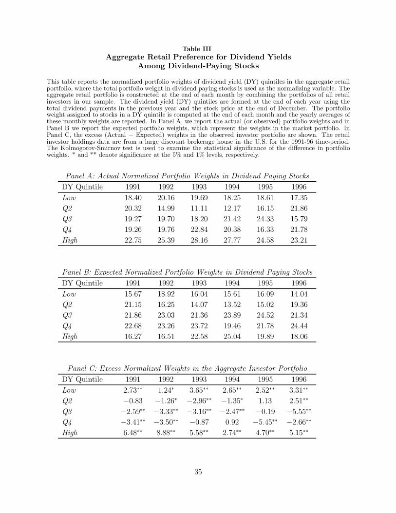
Table III

Aggregate Retail Preference for Dividend Yields

Among Dividend-Paying Stocks

This table reports the normalized portfolio weights of dividend yield (DY) quintiles in the aggregate retailportfolio, where the total portfolio weight in dividend paying stocks is used as the normalizing variable. Theaggregate retail portfolio is constructed at the end of each month by combining the portfolios of all retailinvestors in our sample. The dividend yield (DY) quintiles are formed at the end of each year using thetotal dividend payments in the previous year and the stock price at the end of December. The portfolioweight assigned to stocks in a DY quintile is computed at the end of each month and the yearly averages ofthese monthly weights are reported. In Panel A, we report the actual (or observed) portfolio weights and inPanel B we report the expected portfolio weights, which represent the weights in the market portfolio. InPanel C, the excess (Actual − Expected) weights in the observed investor portfolio are shown. The retailinvestor holdings data are from a large discount brokerage house in the U.S. for the 1991-96 time-period.The Kolmogorov-Smirnov test is used to examine the statistical significance of the difference in portfolioweights. * and ** denote significance at the 5% and 1% levels, respectively.

Panel A: Actual Normalized Portfolio Weights in Dividend Paying Stocks

DY Quintile 1991 1992 1993 1994 1995 1996

Low 18.40 20.16 19.69 18.25 18.61 17.35

Q2 20.32 14.99 11.11 12.17 16.15 21.86

Q3 19.27 19.70 18.20 21.42 24.33 15.79

Q4 19.26 19.76 22.84 20.38 16.33 21.78

High 22.75 25.39 28.16 27.77 24.58 23.21

Panel B: Expected Normalized Portfolio Weights in Dividend Paying Stocks

DY Quintile 1991 1992 1993 1994 1995 1996

Low 15.67 18.92 16.04 15.61 16.09 14.04

Q2 21.15 16.25 14.07 13.52 15.02 19.36

Q3 21.86 23.03 21.36 23.89 24.52 21.34

Q4 22.68 23.26 23.72 19.46 21.78 24.44

High 16.27 16.51 22.58 25.04 19.89 18.06

Panel C: Excess Normalized Weights in the Aggregate Investor Portfolio

DY Quintile 1991 1992 1993 1994 1995 1996

Low 2.73∗∗ 1.24∗ 3.65∗∗ 2.65∗∗ 2.52∗∗ 3.31∗∗

Q2 −0.83 −1.26∗ −2.96∗∗ −1.35∗ 1.13 2.51∗∗

Q3 −2.59∗∗ −3.33∗∗ −3.16∗∗ −2.47∗∗ −0.19 −5.55∗∗

Q4 −3.41∗∗ −3.50∗∗ −0.87 0.92 −5.45∗∗ −2.66∗∗

High 6.48∗∗ 8.88∗∗ 5.58∗∗ 2.74∗∗ 4.70∗∗ 5.15∗∗

35

Table IV

Cross-Sectional Variation in Retail Preference for Dividend-Paying Stocks:

One-Dimensional Sorts

This table reports the total portfolio weights in dividend paying stocks in the aggregate portfolios of threedifferent groups of retail investors, formed on the basis of age, income, and occupation. An aggregateportfolio is constructed for each investor group at the end of each month by combining the portfolios of allretail investors in that category. The portfolio weights in dividend paying stocks are computed at the end ofeach month and the yearly averages of these monthly weights are reported. The portfolio weights in dividendpaying stocks in the aggregate retail portfolio are also shown. The retail investor holdings data are froma large discount brokerage house in the U.S. for the 1991-96 time-period. The Kolmogorov-Smirnov test isused to examine the statistical significance of the difference in portfolio weights. * and ** denote significanceat the 5% and 1% levels, respectively.

Investor Group 1991 1992 1993 1994 1995 1996

All Investors

73.12 70.50 69.48 69.20 68.65 66.01

Age Groups

Below 45 (Younger) 65.82 62.22 59.53 60.15 59.22 57.51

45-65 70.27 69.02 68.06 67.18 66.10 65.42

Above 65 (Older) 81.83 79.73 77.24 76.65 78.50 78.32

Older − Younger 16.01∗∗ 17.50∗∗ 17.71∗∗ 16.50∗∗ 19.29∗∗ 20.81∗∗

Income Groups

Below 40K (Low) 74.71 71.97 68.66 69.04 68.75 66.04

40-75K 71.17 68.76 66.65 66.63 65.50 64.82

Above 75K (High) 70.99 68.90 67.65 67.05 67.65 66.06

Low − High 3.72∗ 3.07∗ 1.01 1.99 1.10 −0.02

Occupation Categories

Professional 68.65 67.85 65.63 64.05 64.43 61.71

Non-Professional 70.06 65.58 62.98 65.02 63.39 66.32

Retired 81.67 80.03 78.58 78.18 78.57 79.41

Retired − Professional 13.02∗∗ 12.18∗∗ 12.95∗∗ 14.13∗∗ 14.14∗∗ 17.70∗∗

36

Table V

Cross-Sectional Variation in Retail Preference for Dividend-Paying Stocks:

Two-Dimensional Sorts

This table reports the total portfolio weights in dividend paying stocks in the aggregate portfolios of ninedifferent groups of retail investors, formed by sorting on age and income. An aggregate portfolio is constructedfor each investor group at the end of each month by combining the portfolios of all retail investors in thatcategory. The portfolio weights in dividend paying stocks are computed at the end of each month andthe yearly averages of these monthly weights are reported. The retail investor holdings data are from alarge discount brokerage house in the US. The Kolmogorov-Smirnov test is used to examine the statisticalsignificance of the difference in portfolio weights. * and ** denote significance at the 5% and 1% levels,respectively.

Age Groups Income Groups 1991 1992 1993 1994 1995 1996

Below 40K (Low) 67.27 62.86 63.44 62.84 60.07 61.38

Younger 40-75K 66.40 62.89 59.66 59.46 57.19 56.30

Above 75K (High) 63.79 60.69 57.70 59.93 61.43 57.78

Low - High 3.48∗ 2.17∗ 5.74∗∗ 2.91∗ −1.36 3.60∗

Below 40K (Low) 72.36 69.30 65.57 66.24 68.79 66.21

Age 45-65 40-75K 68.97 67.82 66.45 66.99 64.70 65.36

Above 75K (High) 71.20 70.31 70.73 67.62 66.98 65.21

Low - High 1.16 −1.01 −5.16∗∗ −1.38 1.81 1.00

Below 40K (Low) 82.92 80.48 78.02 78.54 77.84 78.40

Older 40-75K 81.07 79.12 77.01 74.95 76.99 75.98

Above 75K (High) 82.32 80.41 77.20 78.48 80.92 80.93

Low - High 0.60 0.07 0.82 0.06 −3.08∗ −2.53∗

37

Table VI

Cross-Sectional Variation in Retail Preference for Dividend Yields:One-Dimensional Sorts

This table reports the total weights in the aggregate portfolio of three different groups of investors formedon the basis of age, income, and occupation. The total portfolio weight assigned to stocks in each of thefive dividend yield quintiles is reported. An aggregate portfolio is constructed for each investor group atthe end of each month by combining the portfolios of all retail investors in that category. The dividendyield (DY) quintiles are formed at the end of each year using the total dividend payments in the previousyear and the stock price at the end of December. The total portfolio weight assigned to stocks in a DYquintile is computed at the end of each month and the sample-period averages of these monthly weights arereported. The portfolio weights assigned to stocks in each of the five dividend yield quintiles in the aggregateretail portfolio are also shown. The retail investor holdings data are from a large discount brokerage housein the U.S. for the 1991-96 time-period. The Kolmogorov-Smirnov test is used to examine the statisticalsignificance of the difference in portfolio weights. * and ** denote significance at the 5% and 1% levels,respectively.

Dividend Yield Quintile

Investor Group Low Q2 Q3 Q4 High High−Low

All Investors

19.58 16.10 19.78 20.06 24.48 4.90∗∗

Age Groups

Below 45 (Younger) 24.44 16.93 17.82 18.72 22.09 −2.35∗∗

45-65 21.90 17.76 17.67 19.09 23.58 1.68∗

Above 65 (Older) 16.16 14.18 18.77 19.79 31.09 14.93∗∗

Older − Younger −8.28∗∗ −2.75∗∗ 0.95 1.07 9.00∗∗

Income Groups

Below 40K (Low) 19.23 14.93 17.37 19.45 29.02 9.79∗∗

40-75K 20.15 16.45 18.33 19.60 25.47 5.32∗∗

Above 75K (High) 22.52 17.79 18.24 19.12 22.34 -0.18

Low − High −3.29∗∗ −2.86∗∗ −0.87 0.33 6.68∗∗

Occupation Categories

Professional 26.39 16.78 16.17 17.74 22.91 −3.48∗∗

Non-Professional 21.69 15.34 18.02 20.10 24.85 3.17∗∗

Retired 17.55 16.61 20.11 20.42 25.30 7.74∗∗

Retired − Professional −8.84∗∗ −0.17 3.94∗∗ 2.68∗∗ 2.39∗

38

Table VII

Cross-Sectional Variation in Retail Preference for Dividend Yields:Two-Dimensional Sorts

This table reports the total portfolio weights in the aggregate portfolios of nine different groups of retailinvestors, formed by sorting on age and income. The total portfolio weight assigned to stocks in each ofthe five dividend yield (DY) quintiles is reported. An aggregate portfolio is constructed for each investorgroup at the end of each month by combining the portfolios of all retail investors in that category. Theportfolio weights in dividend paying stocks are computed at the end of each month and the sample-periodaverages of these monthly weights are reported. The retail investor holdings data are from a large discountbrokerage house in the U.S. for the 1991-96 time-period. The Kolmogorov-Smirnov test is used to examinethe statistical significance of the difference in portfolio weights. * and ** denote significance at the 5% and1% levels, respectively.

Dividend Yield Quintile

Age Group Income Group Low Q2 Q3 Q4 High High−Low

Below 40K (Low) 24.65 18.17 17.04 17.39 22.75 −1.90∗

Younger 40-75K 25.73 17.23 17.13 17.94 21.96 −3.77∗∗

Above 75K (High) 22.59 16.31 18.88 20.39 21.83 −0.76

Low − High 2.06∗ 1.86∗ −1.84∗ −3.00∗∗ 0.92

Below 40K (Low) 19.82 15.23 17.27 18.93 28.75 8.93∗∗

Age 45-65 40-75K 20.78 17.27 18.00 19.25 24.69 3.91∗∗

Above 75K (High) 23.87 19.13 17.33 19.00 20.67 −3.20∗∗

Low − High −4.05∗∗ −3.90∗∗ −0.06 −0.07 8.08∗∗

Below 40K (Low) 15.71 12.32 16.79 19.28 35.91 20.20∗∗

Older 40-75K 14.80 13.74 19.23 21.15 31.08 16.28∗∗

Above 75K (High) 18.72 16.54 19.73 17.73 27.28 8.56∗∗

Low − High −3.01∗∗ −4.22∗∗ −2.94∗∗ 1.55∗ 8.63∗∗

39

Table VIII

Portfolio Dividend Yield Across Age and Income Groups

This table reports the average quarterly portfolio dividend yield (in percent) of groups of investors formedby sorting on age and income. The portfolio dividend yield of portfolio p at the end of month t, PDYpt, ismeasured as

PDYpt =

Npt∑

j=1

wpjtDYpjt,

where Npt is the number of stocks in portfolio p at the end of month t, wpjt is the weight of stock j in theportfolio at the end of month t, and DYpjt is the dividend yield of stock j in the portfolio from the mostrecent quarter prior to month t. The annual average of PDY for the 1991-96 sample-period is reported.The retail investor holdings data are from a large discount brokerage house in the U.S. for the 1991-96time-period. The Kolmogorov-Smirnov test is used to examine the statistical significance of the difference inthe average quarterly portfolio yields. * and ** denote significance at the 5% and 1% levels, respectively.

Investor Group 1991 1992 1993 1994 1995 1996

Age Groups

Below 45 (Younger) 0.654 0.560 0.469 0.457 0.440 0.410

45-65 0.667 0.594 0.516 0.508 0.493 0.437

Above 65 (Older) 0.805 0.720 0.631 0.654 0.660 0.600

Older − Younger 0.151∗∗ 0.160∗∗ 0.162∗∗ 0.197∗∗ 0.220∗∗ 0.190∗∗

Income Groups

Below 40K (Low) 0.722 0.655 0.563 0.573 0.572 0.510

40-75K 0.694 0.611 0.530 0.533 0.530 0.494

Above 75K (High) 0.664 0.574 0.491 0.476 0.451 0.398

Low − High 0.058∗∗ 0.082∗∗ 0.072∗∗ 0.097∗∗ 0.122∗∗ 0.112∗∗

40

Table IX

Dividend Preference and Risk Aversion

This table reports the sample-period average quarterly portfolio dividend yield (PDY) for investor groupsformed by performing independent double sorts on age, income, and diversification variables. The portfoliodividend yield of portfolio p at the end of month t, PDYpt, is measured as

PDYpt =

Npt∑

j=1

wpjtDYpjt,

where Npt is the number of stocks in portfolio p at the end of month t, wpjt is the weight of stock j in theportfolio at the end of month t, and DYpjt is the dividend yield of stock j in the portfolio from the mostrecent quarter prior to month t. The diversification level is measured as the sum of squared portfolio weights.It is a proxy for risk aversion. The retail investor holdings data are from a large discount brokerage housein the U.S. for the 1991-96 time-period. The Kolmogorov-Smirnov test is used to examine the statisticalsignificance of the difference in average quarterly portfolio yields. * and ** denote significance at the 5%and 1% levels, respectively.

Diversification Quintiles

Investor Group Low Q2 Q3 Q4 High High−Low

Age Groups

Below 45 (Younger) 0.366 0.386 0.414 0.433 0.448 0.081∗∗

45-65 0.437 0.434 0.440 0.468 0.499 0.062∗∗

Above 65 (Older) 0.617 0.611 0.595 0.600 0.618 0.001

Older − Younger 0.251∗∗ 0.226∗∗ 0.182∗∗ 0.167∗∗ 0.171∗∗

Income Groups

Below 40K (Low) 0.507 0.474 0.477 0.494 0.556 0.048∗

40-75K 0.415 0.441 0.444 0.481 0.505 0.090∗∗

Above 75K (High) 0.379 0.391 0.425 0.444 0.497 0.117∗∗

Low − High 0.128∗∗ 0.083∗∗ 0.051∗ 0.050∗∗ 0.059∗∗

41

Table X

Estimation Results: Household Portfolio Dividend Yield Equation

This table reports the estimates of cross-sectional regressions where the average portfolio dividend yield of ahousehold is the dependent variable and a set of household characteristics are used as independent variables.Income is the total household income, Age is the age of the head of the household, Diversification Levelis the average number of stocks in a household portfolio, and Family Size measures the number of people(children and adults) in the household. The Professional and Retired dummy variables represent occupationcategories, where the professional job category includes investors who hold technical and managerial positions.The remaining investors belong to the non-professional category which consists of blue-collar workers, salesand service workers, and clerical workers. TDA Dummy is set to one if a household holds only tax-deferredaccounts. Portfolio Turnover is the average of monthly buy and sell turnovers, Portfolio Size is the averagesize of the household portfolio, and Portfolio Performance is the risk-adjusted performance (Sharpe Ratio) ofthe household. Finally, RMRF, SMB, HML, and UMD are the factor loadings from a four-factor model wherethe monthly household portfolio return is used to obtain these estimates. To allow for direct comparisonamong the coefficient estimates, variables are standardized so that each variable has a mean of 0 and astandard deviation of 1. The retail investor holdings data are from a large discount brokerage house in theU.S. for the 1991-96 time-period.

Dependent variable: Average portfolio dividend yield (in percent) of a retail investor

1991-93 1994-96 1991-96

Variable Estimate t-stat Estimate t-stat Estimate t-stat

Intercept 0.001 0.05 -0.043 -0.61 -0.000 -0.02

Age 0.069 6.03 0.072 4.66 0.080 6.97

Income -0.022 -2.28 -0.019 -2.44 -0.023 -2.50

Diversification Level 0.018 2.09 0.041 3.15 0.019 2.77

Family Size -0.014 -1.16 0.001 0.12 -0.016 -1.05

Professional Dummy 0.010 0.86 -0.024 -1.70 0.002 0.19

Retired Dummy 0.030 2.39 0.015 1.79 0.028 2.26

TDA Dummy 0.033 3.07 0.010 1.82 0.027 2.91

Portf. Turnover -0.031 -3.24 -0.081 -5.50 -0.032 -3.43

Portf. Size 0.040 3.78 0.023 1.85 0.034 3.20

Portf. Performance 0.044 4.69 0.028 2.59 0.041 4.44

RMRF -0.120 -11.88 -0.141 -9.02 -0.134 -13.65

SMB -0.473 -15.70 -0.559 -13.57 -0.474 -16.28

HML 0.392 16.10 0.439 7.27 0.401 17.55

UMD -0.079 -7.55 -0.008 -0.51 -0.071 -5.88

Num. of households 10,353 6,158 10,457

Adjusted R2 0.24 0.26 0.25

42

Table XI

Trading Behavior Around Ex-Dividend Days

This table reports the average excess buy-sell imbalance (BSI) of groups of retail investors around ex-dividenddates. Investor groups are formed by sorting on age and income. The BSI is computed as the ratio of the netbuy imbalance (Buy Volume − Sell Volume) and the total volume (Buy Volume +Sell Volume) on a givenday. The excess BSI is obtained by subtracting the expected level of BSI where the expected BSI is theaverage of BSI levels on days t−20 to t−16 and days t+16 to t+20. t is the ex-dividend date. Equal-weightedaverages (average is taken across all events) of BSIs are reported for the event date and for four time-periodsaround the ex-dividend date. In Panel A, we report the results for all dividend paying stocks in our sample,in Panel B, we report the average BSIs for low dividend yield stocks (bottom quintile), and in Panel C, wereport the results for high dividend yield (top quintile) stocks. The retail investor holdings data are froma large discount brokerage house in the U.S. for the 1991-96 time-period. The Kolmogorov-Smirnov test isused to examine the statistical significance of the difference in average BSIs. * and ** denote significance atthe 5% and 1% levels, respectively.

Panel A: Ex-Day Activity for All Dividend Yield StocksInvestor Pre-Event EventDay Post-Event Ev−Pre Post−PreGroup -10:-6 -5:-1 0 +1:+5 +6:+10All Investors

-0.81 3.51 2.22 3.22 0.78 −1.29 −0.29

Age GroupsBelow 45 (Younger) -0.88 -0.76 4.41 1.29 -0.02 5.17∗∗ 2.05∗

45-65 -1.36 3.43 -3.61 2.32 1.37 −7.05∗∗ −1.12Above 65 (Older) 2.26 4.10 -1.58 -0.73 -0.74 −5.68∗∗ −4.83∗∗

Older − Younger 3.14∗∗ 4.86∗∗ −5.99∗∗ −2.45∗∗ −0.72 −10.85∗∗ −6.88∗∗

Income GroupsBelow 40K (Low) 1.69 6.61 2.17 2.96 2.04 −4.41∗∗ −3.65∗∗

40-75K -0.54 1.47 -2.17 1.46 -0.50 −3.64∗∗ −0.01Above 75K (High) -1.49 1.12 0.17 0.74 -0.81 −0.94 −0.38

Low − High 3.18∗∗ 5.49∗∗ 2.00∗ 2.22∗ 2.85∗∗ −3.47∗∗ −3.27∗∗

Panel B: Ex-Day Activity for Low Dividend Yield (Bottom DY Quintile) StocksAll Investors

-0.07 0.17 3.27 0.94 -0.36 3.09∗∗ 0.76

Age GroupsBelow 45 (Younger) -1.25 -2.00 0.53 -4.94 -3.91 2.53∗∗ −2.94∗∗

45-65 1.13 0.52 -2.43 -0.87 0.66 −2.96∗∗ −1.40Above 65 (Older) 1.40 -1.54 1.41 -3.81 -0.36 2.95∗∗ −2.27∗∗

Older − Younger 2.65∗∗ 0.46 0.89 1.13 3.55∗∗ 0.42 0.67

Income GroupsBelow 40K (Low) 0.69 0.33 2.08 3.97 0.49 1.75∗ 3.65∗∗

40-75K -0.60 -1.70 -2.70 -3.87 -4.21 −1.00 −2.17∗∗

Above 75K (High) -1.57 -0.66 4.60 -3.85 -3.21 5.26∗∗ −3.19∗∗

Low − High 2.27∗∗ 0.99 −2.52∗∗ 7.82∗∗ 3.70∗∗ −3.51∗∗ 6.84∗∗

Panel C: Ex-Day Activity for High Dividend Yield (Top DY Quintile) StocksAll Investors

0.07 7.85 7.01 7.49 3.87 −0.84 −0.36

Age GroupsBelow 45 (Younger) -2.48 2.77 6.56 6.27 1.29 3.79∗∗ 3.49∗∗

45-65 -1.03 8.17 7.01 7.43 5.17 −1.16 −0.74Above 65 (Older) 6.40 13.26 1.17 1.20 2.66 −12.09∗∗ −12.06∗∗

Older − Younger 8.88∗∗ 10.48∗∗ −5.39∗∗ −5.06∗∗ 1.37 −15.87∗∗ −15.55∗∗

Income GroupsBelow 40K (Low) 4.01 16.45 10.25 3.92 4.15 −6.20∗∗ −12.53∗∗

40-75K 1.84 7.41 3.45 6.02 5.43 −3.95∗∗ −1.39Above 75K (High) -5.59 1.11 2.50 4.35 1.78 1.39 3.24∗∗

Low − High 9.61∗∗ 15.33∗∗ 7.75∗∗ −0.43 2.37∗ −7.58∗∗ −15.77∗∗

43

Table XII

Ex-Day Premium and Retail Investor Characteristics

This table reports the estimated coefficients from pooled regressions with fixed year effects where the de-pendent variable is the average ex-day premium (average taken over the year) for a given stock. The ex-daypremium is defined as the ratio of the ex-day price change (Cum-dividend price − Ex-dividend price) andthe dividend payment. The independent variables are: (i) Age, which is the value-weighted average age ofretail stockholders of a given stock in a particular year, (ii) Income, which is the value-weighted averagehousehold income of retail stockholders of a given stock in a particular year, and (iii) Diversification Level,which is the value-weighted average diversification level of retail stockholders of a given stock in a particularyear. The results under column “All” report the estimates for all dividend paying stocks, while columnsQ1 to Q5 report the estimates for dividend paying stocks in the five size quintiles, respectively. The sizequintiles are formed at the end of each year using the market capitalization at the end of December. The tstatistics for the coefficient estimates are reported in parentheses. The retail investor holdings data are froma large discount brokerage house in the U.S. for the 1991-96 time-period.

Panel A: Unadjusted Ex-Dividend Day Price

Dependent variable: Average Ex-day premium

Size Quintiles

Variable All Small Q2 Q3 Q4 Large

Age 0.007 0.055 0.001 0.003 -0.006 0.005

(1.49) (2.24) (0.01) (0.13) (-0.26) (0.23)

Income -0.006 -0.035 -0.020 0.016 0.003 -0.015

(-1.45) (-1.98) (-0.81) (0.65) (0.11) (-0.77)

Diversification Level -0.015 0.054 -0.001 -0.025 -0.048 -0.045

(-0.94) (1.11) (-0.02) (-0.71) (-1.03) (-1.04)

N(stocks) 9,396 1,766 1,625 1,730 1,939 2,336

Adj. R2 0.002 0.015 0.015 0.006 0.004 0.003

Panel B: Ex-Dividend Day Price Adjusted using CAPM

Size Quintiles

Variable All Small Q2 Q3 Q4 Large

Age 0.009 0.062 0.003 0.017 -0.022 0.020

(1.81) (2.51) (0.13) (0.69) (-0.96) (0.97)

Income -0.005 -0.050 -0.025 0.028 0.011 -0.013

(-1.71) (-2.04) (-0.97) (0.53) (0.48) (-0.61)

Diversification Level -0.015 0.033 0.004 -0.030 -0.055 -0.054

(-0.95) (0.68) (0.11) (-0.84) (-1.15) (-1.09)

N(stocks) 9,396 1,766 1,625 1,730 1,939 2,336

Adj. R2 0.001 0.015 0.019 0.003 0.004 0.004

44

Table XIII

Trading Behavior Around Dividend Announcement Events

This table reports the average excess buy-sell imbalance (BSI) of groups of retail investors around dividendannouncement dates. Investor groups are formed by sorting on age and income. The BSI is computed asthe ratio of the net buy imbalance (Buy Volume − Sell Volume) and the total volume (Buy Volume +SellVolume) on a given day. The excess BSI is obtained by subtracting the expected level of BSI where theexpected BSI is the average of BSI levels on days t − 20 to t − 16 and days t + 16 to t + 20. t is theannouncement date. Equal-weighted averages (average is taken across all events) of excess BSIs are reportedfor the event date and for four time-periods around the announcement date. In Panel A, we report theresults for all dividend paying stocks in our sample, in Panel B, we report the average BSIs for low dividendyield stocks (bottom quintile), and in Panel C, we report the results for high dividend yield (top quintile)stocks. The retail investor holdings data are from a large discount brokerage house in the U.S. for the 1991-96time-period. The Kolmogorov-Smirnov test is used to examine the statistical significance of the differencein average BSIs. * and ** denote significance at the 5% and 1% levels, respectively.

Panel A: Ex-Day Activity for All Dividend Yield StocksInvestor Pre-Event EventDay Post-Event Ev−Pre Post−PreGroup -10:-6 -5:-1 0 +1:+5 +6:+10All Investors

-0.97 -0.76 1.05 2.90 0.92 1.80∗ 3.65∗∗

Age GroupsBelow 45 (Younger) -2.11 0.50 0.23 0.68 -0.66 −0.27 0.1845-65 -0.97 -1.73 1.13 1.24 -0.73 2.85∗∗ 2.96∗∗

Above 65 (Older) -0.51 1.23 2.20 6.34 1.42 0.97 5.11∗∗

Older − Younger 1.60 0.73 1.97∗ 5.67∗∗ 2.08∗ 1.24 4.93∗∗

Income GroupsBelow 40K (Low) -0.45 0.36 1.22 3.70 0.89 0.87 3.34∗∗

40-75K -1.94 0.89 1.05 2.99 -1.21 0.17 2.10∗∗

Above 75K (High) -0.81 -2.06 -1.45 -0.99 1.15 0.61 1.07

Low − High 0.36 2.42∗∗ 2.68∗∗ 4.69∗∗ −0.25 0.26 2.27∗∗

Panel B: Ex-Day Activity for Low Dividend Yield (Bottom DY Quintile) StocksAll Investors

-3.47 -2.48 1.94 1.77 -1.36 4.42∗∗ 4.25∗∗

Age GroupsBelow 45 (Younger) -5.35 -2.21 4.89 0.67 -5.01 7.10∗∗ 2.88∗∗

45-65 -3.26 -1.98 7.00 0.57 -3.14 8.99∗∗ 2.56∗∗

Above 65 (Older) -3.31 1.79 4.28 6.46 -4.31 2.49∗∗ 4.67∗∗

Older − Younger 2.04∗ 4.00∗∗ −9.17∗∗ 5.79∗∗ 0.70 −4.61∗∗ 1.79∗

Income GroupsBelow 40K (Low) -6.03 -3.57 4.00 1.91 -4.73 7.57∗∗ 5.48∗∗

40-75K -6.37 0.16 5.72 1.89 -6.52 5.56∗∗ 1.72∗

Above 75K (High) -0.92 -2.46 5.27 4.11 2.51 7.72∗∗ 6.57∗∗

Low − High −5.11∗∗ −1.12 −1.27 −2.20∗∗ −7.25∗∗ −0.15 −1.09

Panel C: Ex-Day Activity for High Dividend Yield (Top DY Quintile) StocksAll Investors

1.68 -1.79 2.03 4.06 3.64 3.82∗∗ 5.85∗∗

Age GroupsBelow 45 (Younger) 1.96 0.62 1.85 -0.93 0.07 1.24 −1.5445-65 -0.60 -5.54 -4.57 0.68 -2.33 0.97 6.21∗∗

Above 65 (Older) 1.39 1.71 9.64 13.06 10.37 7.93∗∗ 11.35∗∗

Older − Younger 0.57 1.09 7.79∗∗ 13.99∗∗ 10.30∗∗ 6.69∗∗ 12.89∗∗

Income GroupsBelow 40K (Low) 2.42 2.44 5.29 5.76 7.48 2.84∗∗ 3.32∗∗

40-75K 1.37 -2.15 -0.10 3.87 0.44 2.06∗ 6.02∗∗

Above 75K (High) 2.10 -1.91 -4.58 -1.81 1.04 −2.67∗∗ 0.10

Low − High 0.32 4.36∗∗ 9.87∗∗ 7.57∗∗ 6.45∗∗ 5.52∗∗ 3.22∗∗

45

Table XIV

Retail Ownership Shifts Around Dividend Initiations and Omissions

This table reports the total and excess group ownership around dividend initiation and omission events.Investor groups are defined based on age and income. The total ownership of an investor group in a particularstock is the total weight of the stock in the aggregate group portfolio, where the aggregate group portfoliois constructed by combining the portfolios or all investors within the group. Corresponding to each event, abenchmark ownership level is also defined for each group where the benchmark ownership level is assumedto be the average ownership in months t − 7 to t − 2 and t is the event month. The excess ownership isthe difference between the observed and benchmark ownership levels. Column 1 reports the benchmarkownership levels, columns 2-5 report the observed ownership levels, and columns 6-8 report excess ownershiplevels. The retail investor holdings data are from a large discount brokerage house in the U.S. for the 1991-96time-period. The Kolmogorov-Smirnov test is used to examine the statistical significance of the differencein average BSIs. * and ** denote significance at the 5% and 1% levels, respectively.

Panel A: Dividend InitiationsInvestor Pre(2) Pre(1) Ev Post(1) Post(2) Ev− Post(1)− Post(2)−Group (-7:-2) (-1) (0) (+1) (+2:+7) Pre(2) Pre(2) Pre(2)All Investors

1.67 1.73 1.78 1.63 1.67 0.11∗ -0.04 -0.01

Age GroupsBelow 45 (Younger) 1.85 1.96 1.89 1.90 1.82 0.04 0.05 -0.0245-65 1.67 1.69 1.68 1.62 1.59 0.01 -0.05 -0.08Above 65 (Older) 1.90 1.97 2.08 2.17 1.98 0.18∗∗ 0.28∗∗ 0.09∗

Income GroupsBelow 40K (Low) 1.70 1.74 1.84 1.95 1.70 0.14∗ 0.25∗∗ -0.0040-75K 1.89 1.89 1.98 1.89 1.76 0.09∗ 0.01 −0.13∗

Above 75K (High) 1.74 1.86 1.78 1.76 1.70 0.04 0.02 -0.04

Panel B: Dividend OmissionsInvestor Pre(2) Pre(1) Ev Post(1) Post(2) Ev− Post(1)− Post(2)−Group (-7:-2) (-1) (0) (+1) (+2:+7) Pre(2) Pre(2) Pre(2)All Investors

1.57 1.53 1.51 1.55 1.54 -0.05 -0.02 -0.02

Age GroupsBelow 45 (Younger) 1.86 1.93 2.00 2.11 1.94 0.14∗∗ 0.25∗∗ 0.0845-65 1.68 1.63 1.86 1.70 1.60 0.18∗∗ 0.02 -0.08Above 65 (Older) 1.87 2.08 1.93 1.79 1.92 0.06 −0.08 0.05

Income GroupsBelow 40K (Low) 2.15 1.94 2.05 1.93 1.83 −0.10∗ −0.22∗∗ −0.32∗∗

40-75K 1.48 1.52 1.49 1.48 1.51 0.01 0.00 0.03Above 75K (High) 1.84 1.67 1.88 1.61 1.50 0.05 −0.23∗∗ −0.34∗∗

46

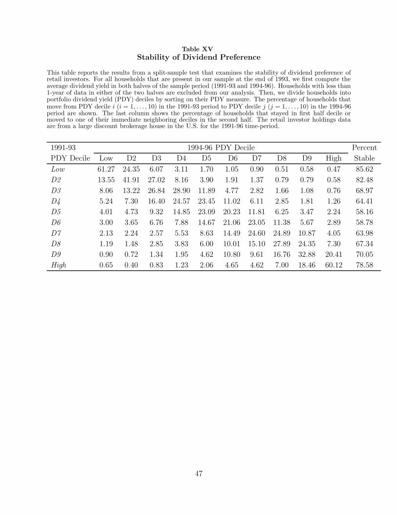
Table XV

Stability of Dividend Preference

This table reports the results from a split-sample test that examines the stability of dividend preference ofretail investors. For all households that are present in our sample at the end of 1993, we first compute theaverage dividend yield in both halves of the sample period (1991-93 and 1994-96). Households with less than1-year of data in either of the two halves are excluded from our analysis. Then, we divide households intoportfolio dividend yield (PDY) deciles by sorting on their PDY measure. The percentage of households thatmove from PDY decile i (i = 1, . . . , 10) in the 1991-93 period to PDY decile j (j = 1, . . . , 10) in the 1994-96period are shown. The last column shows the percentage of households that stayed in first half decile ormoved to one of their immediate neighboring deciles in the second half. The retail investor holdings dataare from a large discount brokerage house in the U.S. for the 1991-96 time-period.

1991-93 1994-96 PDY Decile Percent

PDY Decile Low D2 D3 D4 D5 D6 D7 D8 D9 High Stable

Low 61.27 24.35 6.07 3.11 1.70 1.05 0.90 0.51 0.58 0.47 85.62

D2 13.55 41.91 27.02 8.16 3.90 1.91 1.37 0.79 0.79 0.58 82.48

D3 8.06 13.22 26.84 28.90 11.89 4.77 2.82 1.66 1.08 0.76 68.97

D4 5.24 7.30 16.40 24.57 23.45 11.02 6.11 2.85 1.81 1.26 64.41

D5 4.01 4.73 9.32 14.85 23.09 20.23 11.81 6.25 3.47 2.24 58.16

D6 3.00 3.65 6.76 7.88 14.67 21.06 23.05 11.38 5.67 2.89 58.78

D7 2.13 2.24 2.57 5.53 8.63 14.49 24.60 24.89 10.87 4.05 63.98

D8 1.19 1.48 2.85 3.83 6.00 10.01 15.10 27.89 24.35 7.30 67.34

D9 0.90 0.72 1.34 1.95 4.62 10.80 9.61 16.76 32.88 20.41 70.05

High 0.65 0.40 0.83 1.23 2.06 4.65 4.62 7.00 18.46 60.12 78.58

47

Table XVI

Dividend Preference and the Disposition Effect

This table reports disposition effect (DE) measures for investor groups formed by sorting on age and income.The DE is computed for each of the five DY quintiles. The DE measure is defined as the difference ofproportion of gains realized (PGR) and proportion of losses realized (PLR). PGR is the ratio of the numberof gains realized and the total number of winners in a given portfolio (i.e, the total number of actual gainsand paper gains). Similarly, PLR is the ratio of the number of losses realized and the total number of losers ina given portfolio (i.e, the total number of actual losses and paper losses). Therefore, a positive DE indicatesthat the investor is less willing to sell the losers in the portfolio relative to the winners in the portfolio. Theretail investor holdings data is from a large discount brokerage house in the U.S. for the 1991-96 time-period.The Kolmogorov-Smirnov test is used to examine the statistical significance of the difference in the averageDE. * and ** denote significance at the 5% and 1% levels, respectively.

Dividend Yield (DY) Quintiles

Investor Group Low Q2 Q3 Q4 High High−Low

All Investors

0.043 0.030 0.026 0.035 0.029 −0.014∗∗

Age Groups

Below 45 (Younger) 0.085 0.068 0.060 0.075 0.059 −0.026∗∗

45-65 0.056 0.045 0.039 0.045 0.039 −0.017∗∗

Above 65 (Older) 0.023 0.016 0.017 0.016 0.007 −0.016∗∗

Income Groups

Below 40K (Low) 0.055 0.040 0.047 0.049 0.039 −0.017∗∗

40-75K 0.058 0.052 0.041 0.048 0.038 −0.020∗∗

Above 75K (High) 0.054 0.035 0.029 0.035 0.027 −0.027∗∗

Diversification Groups

Low Div 0.121 0.098 0.082 0.081 0.087 −0.034∗∗

Medium Div 0.109 0.069 0.076 0.071 0.073 −0.036∗∗

High Div 0.030 0.023 0.021 0.028 0.022 −0.008∗

48

Table XVII

Cross-Sectional Variation in Dividend Preference at the Time of Purchase

This table reports the value-weighted average quarterly dividend yield of stocks purchased by different groupsof retail investors formed on the basis of their age, income, and occupation. The dividend yield from themost recent quarter prior to a trade is used to compute the average yields where the weights are determinedby the dollar value of the trades. The results are qualitatively similar when all trades are weighted equally.The retail investor holdings data are from a large discount brokerage house in the U.S. for the 1991-96time-period. The Kolmogorov-Smirnov test is used to examine the statistical significance of the differencein portfolio weights. * and ** denote significance at the 5% and 1% levels, respectively.

1991 1992 1993 1994 1995 1996

Age Groups

Below 45 (Younger) 0.350 0.313 0.232 0.253 0.162 0.176

45-65 0.415 0.408 0.334 0.349 0.238 0.241

Above 65 (Older) 0.581 0.580 0.448 0.491 0.332 0.375

Older − Younger 0.231∗∗ 0.266∗∗ 0.216∗∗ 0.238∗∗ 0.169∗∗ 0.200∗∗

Income Groups

Below 40K (Low) 0.475 0.419 0.326 0.361 0.282 0.239

40-75K 0.422 0.377 0.306 0.329 0.229 0.215

Above 75K (High) 0.410 0.375 0.303 0.330 0.232 0.228

Low − High 0.065∗∗ 0.044∗∗ 0.023∗ 0.032∗ 0.051∗∗ 0.011

Occupation Categories

Professional 0.420 0.372 0.301 0.331 0.236 0.220

Non-Professional 0.413 0.387 0.314 0.342 0.241 0.219

Retired 0.544 0.491 0.405 0.443 0.325 0.317

Retired − Professional 0.124∗∗ 0.119∗∗ 0.104∗∗ 0.112∗∗ 0.089∗∗ 0.096∗∗

49

Jan 91 Jan 92 Jan 93 Jan 94 Jan 95 Jan 96

0.4

0.5

0.6

0.7

0.8

0.9

1

Age: Below 45

Age: 45−65

Age: Above 65

Date (Jan 1991 − Nov 1996)

Avg

Por

tfolio

Div

iden

d Y

ield

(in

Per

cent

)

Figure 1. Dividend Preference and Age. This figure shows the time-variation in the quarterly portfoliodividend yield of three groups of investors grouped as age cohorts. The portfolio dividend yield of a givenportfolio is measured as the weighted average of the dividend yields of all stocks in the portfolio. TheKolmogorov-Smirnov test is used to examine the statistical significance of the difference in portfolio weights.

50

Jan 91 Jan 92 Jan 93 Jan 94 Jan 95 Jan 96

0.4

0.5

0.6

0.7

0.8

0.9

Income: Below 40K

Income: 40−75K

Income: Above 75K

Date (Jan 1991 − Nov 1996)

Avg

Por

tfolio

Div

iden

d Y

ield

(in

Per

cent

)

Figure 2. Dividend Preference and Income. This figure shows the time-variation in the portfoliodividend yield of three groups of investors grouped as income cohorts. The portfolio dividend yield of agiven portfolio is measured as the weighted average of the dividend yields of all stocks in the portfolio. TheKolmogorov-Smirnov test is used to examine the statistical significance of the difference in portfolio weights.

51

0.3

0.4

0.5

0.6

0.7

0.8

0.9(a) High Income Households

Avg

PD

Y (

in P

erce

nt)

0.3

0.4

0.5

0.6

0.7

0.8

0.9(b) Low Income Households

Jan 91Jan 92Jan 93Jan 94Jan 95Jan 960.3

0.4

0.5

0.6

0.7

0.8

0.9(c) Younger Households

Date (Jan 1991 − Nov 1996)

Avg

PD

Y (

in P

erce

nt)

Jan 91Jan 92Jan 93Jan 94Jan 95Jan 960.3

0.4

0.5

0.6

0.7

0.8

0.9(d) Older Households

Date (Jan 1991 − Nov 1996)

Tax−deferredTaxable

Figure 3. Dividend Preference in taxable and tax-deferred accounts. This figure shows thetime-variation in the average quarterly portfolio dividend yield of investors who hold only taxable accountsor only tax-deferred accounts. Four groups of investors are examined: (a) high-income, (b) low-income, (c)younger, and (d) older. The portfolio dividend yield of a given portfolio is measured as the weighted averageof the dividend yields of all stocks in the portfolio. The Kolmogorov-Smirnov test is used to examine thestatistical significance of the difference in portfolio weights.

52