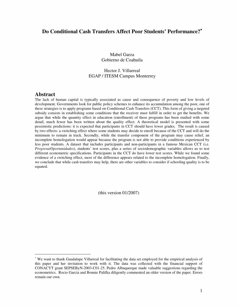
1

Do Conditional Cash Transfers Affect Poor Students’ Performance?∗∗∗∗

Mabel Garza Gobierno de Coahuila

Hector J. Villarreal

EGAP / ITESM Campus Monterrey

Abstract The lack of human capital is typically associated as cause and consequence of poverty and low levels of development. Governments look for public policy schemes to enhance its accumulation among the poor, one of these strategies is to apply programs based on Conditional Cash Transfers (CCT). This form of giving a targeted subsidy consists in establishing some conditions that the receiver must fulfill in order to get the benefits. We argue that while the quantity effect in education (enrollment) of these programs has been studied with some detail, much fewer has been written about the quality effect. A theoretical model is presented with some pessimistic predictions: it is expected that participants in CCT should have lower grades. The result is caused by two effects: a switching effect where some students may decide to enroll because of the CCT and will do the minimum to remain in track. Secondly, while the transfer component of the program may cause relief, an incomplete homologation would appear because the program is not able to provide conditions experienced by less poor students. A dataset that includes participants and non-participants in a famous Mexican CCT (i.e. Progresa/Oportunidades), students’ test scores, plus a series of sociodemographic variables allows us to test different econometric specifications. Participants in the CCT do have lower test scores. While we found some evidence of a switching effect, most of the difference appears related to the incomplete homologation. Finally, we conclude that while cash transfers may help, there are other variables to consider if schooling quality is to be equated.

(this version 01/2007)

∗ We want to thank Guadalupe Villarreal for facilitating the data set employed for the empirical analysis of this paper and her invitation to work with it. The data was collected with the financial support of CONACYT grant SEPSEByN-2003-C01-25. Pedro Albuquerque made valuable suggestions regarding the econometrics. Rocio Garcia and Bonnie Palifka diligently commented an older version of the paper. Errors remain our own.

2

I. Introduction

The lack of human capital is typically associated as a cause and consequence of poverty and

underdevelopment. The fact that low-income households invest very little on education and

health tends to perpetuate poverty via vicious circles, i.e. poverty traps. As a response, the

last two decades have witnessed the emergence of a series of Conditional Cash Transfers

programs (CCT), (Lindert, Skoufias, and Shapiro 2005; Das, Do, and Özler 2004, 2005;

Bourguignon, Ferreira, and Leite 2003; Rawlings and Rubio 2005). These programs possess

two peculiarities described in their name. On the one hand, CCT involve direct cash transfers

as opposed to in kind transfers or to subsidies of particular goods. In theory, the “cash

transfer” element is associated with short-run welfare alleviation. The second characteristic is

that reception of resources implies the commitment of the household to follow certain

behavior (school attendance by children, medical check-ups, etc.). The objective within this

second element is to align incentives in order for poor households to accumulate human

capital. Thus, this second element is expected to enhance welfare in the longer run.

Several evaluations and assessments of CCT have shown positive effects with respect

to human capital acquisition by participants in the programs, (Behrman, Sengupta, and Todd

2000; Gertler and Fernald 2004). In particular, CCT appear quite successful incrementing

schooling among the poor (enrollment), (Schultz 2000; Skoufias and Parker 2001; Behrman,

Parker, and Todd 2004). The fact that this type of programs permits good targeting enables

them as an efficient tool for social policy, (Lindert, Skoufias, and Shapiro 2005; Das, Do, and

Özler 2004). While the “quantity” component of the acquired human capital has been studied

to a considerable extent, much less has been said about the “quality” component. The issue is

far from trivial, if the quality component is not considered the accumulation of human capital

3

may be overestimated (underestimated). With respect to schooling, the latter may have a

profound effect for productivity, the acquisition of further human capital, and signaling in the

labor markets.

In this paper, we investigate the effects of CCT on poor students’ performance. We

believe students’ academic performance (SAP) is a good proxy of the quality of the acquired

human capital. A sensible hypothesis is that CCT do not have a direct effect on SAP once the

poverty level of the household is controlled. However, to the extent that these programs

affect variables that influence SAP, important indirect effects may show up. Moreover,

standard revealed preference logic suggests that the indirect effects may be negative. This

would be bad news, as it implies that that the accumulation of human capital by the poor

facilitated with CCT is overrated.

The paper is organized in the following way. Section II introduces a model of grade

formation and educational investment. The role of costs and expectations is studied as well as

the influence that the aforementioned social programs may have on them. Section III presents

the data; we have a sample of 1243 ninth grade students in Mexico and their exam results in

several subjects. A subset of these students participates in a famous Mexican CCT, i.e.

Progresa/Oportunidades. The availability of a rich set of sociodemographic and personal

variables allows us to test the model presented previously. In section IV the estimation

strategy is described, the econometric results presented and some implications suggested.

Finally, section V concludes and succinctly motivates some avenues for future research.

II.Theoretical Model

We begin by describing the formation of grades (the proxy we are using to describe the

quality of human capital):

4

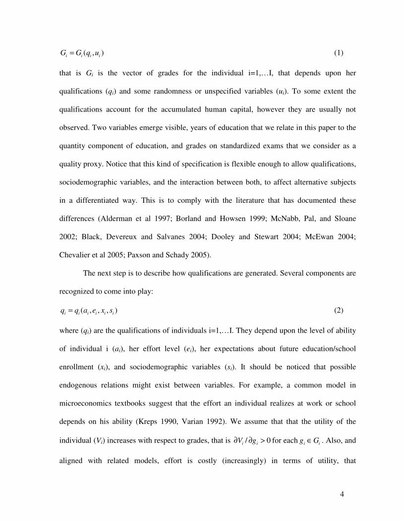
( , )i i i iG G q u= (1)

that is Gi is the vector of grades for the individual i=1,…I, that depends upon her

qualifications (qi) and some randomness or unspecified variables (ui). To some extent the

qualifications account for the accumulated human capital, however they are usually not

observed. Two variables emerge visible, years of education that we relate in this paper to the

quantity component of education, and grades on standardized exams that we consider as a

quality proxy. Notice that this kind of specification is flexible enough to allow qualifications,

sociodemographic variables, and the interaction between both, to affect alternative subjects

in a differentiated way. This is to comply with the literature that has documented these

differences (Alderman et al 1997; Borland and Howsen 1999; McNabb, Pal, and Sloane

2002; Black, Devereux and Salvanes 2004; Dooley and Stewart 2004; McEwan 2004;

Chevalier et al 2005; Paxson and Schady 2005).

The next step is to describe how qualifications are generated. Several components are

recognized to come into play:

( , , , )i i i i i iq q a e x s= (2)

where (qi) are the qualifications of individuals i=1,…I. They depend upon the level of ability

of individual i (ai), her effort level (ei), her expectations about future education/school

enrollment (xi), and sociodemographic variables (si). It should be noticed that possible

endogenous relations might exist between variables. For example, a common model in

microeconomics textbooks suggest that the effort an individual realizes at work or school

depends on his ability (Kreps 1990, Varian 1992). We assume that that the utility of the

individual (Vi) increases with respect to grades, that is 0/ >∂∂ ii gV for each i ig G∈ . Also, and

aligned with related models, effort is costly (increasingly) in terms of utility, that

5

is 2 2/ 0, / 0i i i iV e V e∂ ∂ < ∂ ∂ < , (De Fraja and Oliveira 2005)1. As these authors mention, the

effort is not necessarily limited to students themselves. To the extent that costs are involved,

any behavior by other members of the family or household can be considered part of the

educational effort, which will be discussed below.

We define a human capital function that considers both the quantity (years of

schooling) and quality (grades) components:2

( , | 1,..., )i i i ij iK K y G j y= = (3)

so the human capital of a person depends on her years of schooling (yi) and the grades

received at each academic year j , (Gij). Notice, this does not mean that the grades of each

school year have an equal weight, i.e. it is very plausible that the grades at the last year are

more important.

Educational Investment

The next step is to link the formation of human capital at the individual level with the

household framework and circumstances. To understand the accumulation of human capital

by the household we propose a model of educational investment inspired in (Brown and Park

2001). Define:

( ) [(1 ) ( ) ( )]

. .

i

i i i i ie

i i

MaxW I C R K A R K M V

s t I b C N

α α

−

= − + + − +

+ ≥ +

(4)

1 It is a common practice in this kind of models to assume that the utility generated and the costs can be separated into two distinct functions. In that case the cost function is usually assumed to be convex. Both the separability and convexity of the cost function do not stem from economic theory. However, it is very convenient to use that framework to guarantee well-behaved solutions. For a good discussion, please refer to Kreps (1990). 2 To the extent that standardized tests are available, grades may be a sensible measurement of the quality component across schools, regions, etc.

6

that is the household tries to maximize its utility or well-being (W)3. We define (Ii) as the

potential income of the household, and assume it is a function of a set of variables (Zi). The

function (Ci) takes into account the costs of children attending school; it includes opportunity

costs (forgone wages), school fees, and related costs such as transportation or school

materials. R(Ki) is the present value of the income flows for particular human capital profiles,

part of it will be kept by the individuals, and part of it will be transferred to the parents (α ∈

[0,1]). The function (A) measures the degree of altruism of the parents (explained below),

meanwhile M(Vi) is the present money metric utility value of the school experience. Finally,

a standard budget constraint is augmented with a borrowing constraint b−

(truncated because

imperfect markets and poverty), and a minimum consumption level (N).

The level of altruism can depend upon a series of variables; among them, the gender

of children tends to play a critical role. However, this effect may not necessarily be uniform

across regions, rural/urban areas, economic levels, etc. The existent literature has sought to at

least partially explain the altruism rationale as intra household bargaining, (Brown and Park

2001; Browning, Chiappori, and Lewbel 2005). Therefore, we proceed to model the

parameter ( A∈ [0, 1]) as:

( , , )f m

i i i iA A s l l= (5)

where (si) is a set of sociodemographic characteristics, and ( ,f m

i il l ) are the educational levels

of the father and the mother respectively.

Now, we should consider the investment problem of the household that participates in

the CCT:

3 Notice that while equations 1-3 refer to an individual, the investment decision is at the household level. Of course the presence of more than one child in the household can create several complementarities that are omitted here. The later is equivalent to assume that there is only one child per household or that the W’s as presented can be added through children.

7

( ) [(1 ) ( ) ( )]

. . ,

i

i i i i i ie

o

i i i i

MaxW I C T R K A R K M V

s t I b T C N e e

α α

−

= − + + + − +

+ + ≥ + ≥

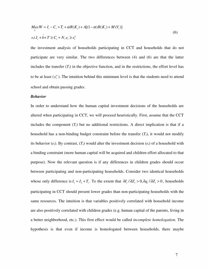
(6)

the investment analysis of households participating in CCT and households that do not

participate are very similar. The two differences between (4) and (6) are that the latter

includes the transfer (Ti) in the objective function, and in the restrictions, the effort level has

to be at least ( o

ie ). The intuition behind this minimum level is that the students need to attend

school and obtain passing grades.

Behavior

In order to understand how the human capital investment decisions of the households are

altered when participating in CCT, we will proceed heuristically. First, assume that the CCT

includes the component (Ti) but no additional restrictions. A direct implication is that if a

household has a non-binding budget constraint before the transfer (Ti), it would not modify

its behavior (ei). By contrast, (Ti) would alter the investment decision (ei) of a household with

a binding constraint (more human capital will be acquired and children effort allocated to that

purpose). Now the relevant question is if any differences in children grades should occur

between participating and non-participating households. Consider two identical households

whose only difference is 1 2 iI I T= + . To the extent that / 0, / 0i i i iI Z q Z∂ ∂ > ∂ ∂ > , households

participating in CCT should present lower grades than non-participating households with the

same resources. The intuition is that variables positively correlated with household income

are also positively correlated with children grades (e.g. human capital of the parents, living in

a better neighborhood, etc.). This first effect would be called incomplete homologation. The

hypothesis is that even if income is homologated between households, there maybe

8

characteristics affecting both income and qualifications that are not homologated by CCT,

thus non-participating children have better grades.

Now we would consider the effort constraint of CCT. Assume that

0( ( ) [(1 ) ( ) ( )] | ) 0i i i i iC R K A R K M V eα α− + + − + < . Many factors can be producing the result:

high opportunity costs, poor expectations, low level of ability by the students, etc. A

truncation result occurs and children would not do that extra school year. We will call

children under that condition type 1, children with the inequality positive will be catalogued

as type 2. Now, children participating the described CCT have to attend school, an

implication of the model is that 0( ( ) [(1 ) ( ) ( )] | ) 0i i i i i iC R K A R K M V e Tα α− + + − + + > . Notice

that by the convexity assumption, if a child was type 1 and now participates in CCT her

effort level must be ( o

ie ). If some of the children participating in CCT were type 1, type 2

children have * 0i ie e> where *

ie solves the investment problems, and / 0i iq T∂ ∂ = ; then grades

from children participating in CCT would be lower other things equal.4 This second effect

would be called switching. The hypothesis is that some children would not study without

CCT because of opportunity costs. The transfer component (Ti) would make them switch, but

they would try to minimize effort. These children should have lower average grades

compared to non-switchers.

Under the model developed in this section, both the incomplete homologation and the

switching effects, suggest that the children participating in CCT would have lower grades on

average than non-participants.

III. The Empirical Environment

4 These are sufficient conditions, necessary conditions are much weaker.

9

The Mexican government created in 1997 the Programa de Educación, Salud y Alimentación

(Progresa). The driving idea was that education is the key to break the vicious cycle of

poverty and that unless the minimum conditions on health and nutrition are satisfied, the

benefits of education will be suboptimal, and therefore poverty would continue. According to

an evaluation made by the Mexican Ministry of Social Development, by the end of the year

2000, the program counted with more than 2.4 millions of families as beneficiaries, living in

53,000 rural communities in 31 states. The program was mildly reformulated and renamed in

year 2002 as Programa de Desarrollo Humano Oportunidades (Oportunidades). Among the

changes there was the inclusion of urban and semi-urban communities (previously it was

limited to rural areas), the promotion of jobs for participants, and access to basic financial

services. By the end of 2005, five million families were beneficiaries from the program.5

One of the distinguishing factors of Progresa/Oportunidades is that it is a conditional

cash transfer program (CCT), which means than once a family has been selected to

participate in the program, they have to fulfill certain requirements in order to keep receiving

the transfers. Particularly on the educational component, the scholarships and economic help

to buy school supplies are granted for children in school age, specifically for those from the

third to the last grade of secondary school (ninth grade). The amount of cash increases as the

child moves from one year to the next. When the child reaches the seventh grade, the transfer

is greater for girls than for boys. The motivation for this is that desertion from school is

greater for girls than for boys during secondary school. The transfer for education is

conditioned to the attendance of children to the school and the participation of the parents in

school activities. Unjustified absences lead to the loss of the scholarship.

5 Source: Sedesol, La Política Social del Gobierno de México, resultados 1995-2000 y retos futuros (http://www.sedesol.gob.mx/)

10

Participant’s Selection

In order to determine who would participate in the program, three steps were covered. In the

first place, the Ministry of Social Development (Sedesol) determined the geographic areas

with the most critical conditions of poverty and their access to health and educational

services. Once those areas were identified, the second step was to recollect socioeconomic

data about the families in the area, to determine which should have been beneficiaries of the

transfers. The third and last step was to present in the community assembly6 the list of the

selected families in order to receive feedback, further suggestions and reasons to include any

other family in the program.

Another difference between Progresa and Oportunidades lies in the selection method.

With the addition of families from urban and semi-urban areas, the existent method could not

be used due to excessive costs. For these cases, they adopted an alternative method of sign-

up modules. The problem of this strategy is that some families that should have been selected

maybe were not because they did not sing up (Parker, Todd, and Wolpin 2005).

Previous Evaluations

Shultz (2000) showed that Progresa has had a positive effect in the enrollment in primary

and secondary schools for both boys and girls. At the secondary school level, the enrollment

rates were 67% for girls and 73% before Progresa. Just a couple of years after the program

began the enrollment had an increase of above 8% for the boy’s case and of 14% for the

girls. He also found that the Program itself contributes with .66 years of additional years of

schooling for both sexes. If analyzed separately, the increase in the years of education is

6 Community Assembly is a reunion of the population of a rural community in which the members discuss public matters; in this case, the participation of certain families in the Program.

11

greater for girls than for boys. The former have a gain of .72 years of additional education

and the latter of .64 years.

Concerning to dropout rates, Behrman, Sengupta, and Todd (2005) found that

students with a Progresa educational grant have lower dropout rates and higher school re-

entry rates among those who had dropped-out. They also found that the program has a special

effectiveness in the dropout reduction during the transition from sixth to seventh grade.

A previous evaluation of the impact of Progresa on school performance was

conducted by the same authors (Behrman, Sengupta, and Todd 2000). They evaluated the

Program after a school year and a half of exposition to the program and they found no

significant impact on improving student scores but they also recognized the limitations due to

the available data they had and the exposure time to the Program.

The Data Employed in This Paper

The dataset includes 1255 students that finished middle school in 2005, and is drawn from a

survey conducted in April of the same year by Dr. Guadalupe Villarreal. The dataset contains

information about students of two states, Chiapas and Nuevo León, studying in two types of

schools, telesecondarys and general secondary schools. The students in the survey took an

EXANI I test and filled a registry form to obtain sociodemographic data.

Telesecondary is a distance education format available in rural communities in which

the student instead of having a teacher receives the classes through television. This system

has come to alleviate the problem of the shortage of middle school institutions and teachers

in isolated communities. The general middle school is the traditional format institution where

the teacher gives the classes directly to the students.

12

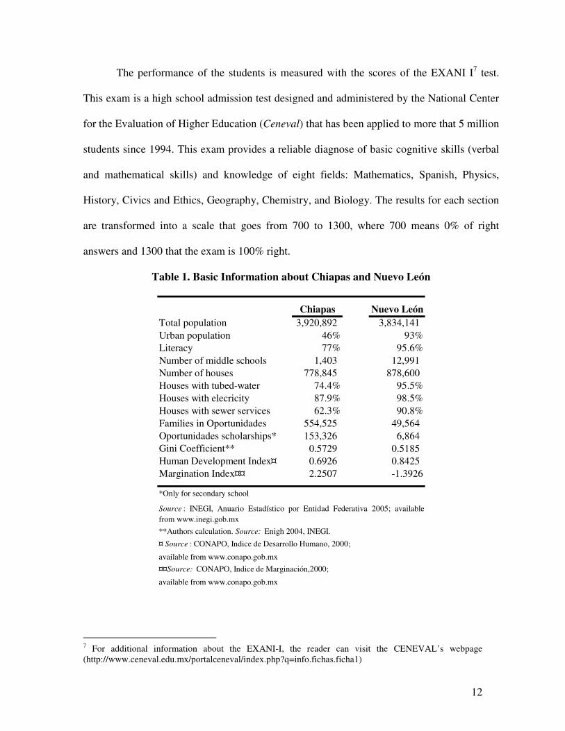
The performance of the students is measured with the scores of the EXANI I7 test.

This exam is a high school admission test designed and administered by the National Center

for the Evaluation of Higher Education (Ceneval) that has been applied to more that 5 million

students since 1994. This exam provides a reliable diagnose of basic cognitive skills (verbal

and mathematical skills) and knowledge of eight fields: Mathematics, Spanish, Physics,

History, Civics and Ethics, Geography, Chemistry, and Biology. The results for each section

are transformed into a scale that goes from 700 to 1300, where 700 means 0% of right

answers and 1300 that the exam is 100% right.

Table 1. Basic Information about Chiapas and Nuevo León

Chiapas Nuevo León

Total population 3,920,892 3,834,141 Urban population 46% 93%Literacy 77% 95.6%Number of middle schools 1,403 12,991 Number of houses 778,845 878,600 Houses with tubed-water 74.4% 95.5%Houses with elecricity 87.9% 98.5%Houses with sewer services 62.3% 90.8%Families in Oportunidades 554,525 49,564 Oportunidades scholarships* 153,326 6,864 Gini Coefficient** 0.5729 0.5185 Human Development Index¤ 0.6926 0.8425 Margination Index¤¤ 2.2507 -1.3926

*Only for secondary school

**Authors calculation. Source: Enigh 2004, INEGI.

¤ Source : CONAPO, Indice de Desarrollo Humano, 2000;

available from www.conapo.gob.mx

¤¤Source: CONAPO, Indice de Marginación,2000;

available from www.conapo.gob.mx

Source : INEGI, Anuario Estadístico por Entidad Federativa 2005; availablefrom www.inegi.gob.mx

7 For additional information about the EXANI-I, the reader can visit the CENEVAL’s webpage (http://www.ceneval.edu.mx/portalceneval/index.php?q=info.fichas.ficha1)

13

Chiapas and Nuevo León present great differences. While the first state has 54% of

rural population, the second only has 7%. The GDP in Nuevo León is 45,759.7848 million

dollar compared to 10,441.6316 million dollar in Chiapas.8 There are also big differences

among the number of families that are part of Oportunidades and the basic services that the

households have available (Table 1).

IV. Estimation Strategy and Econometric Analysis

Table 2 presents the average scores in different subjects for students in the sample: both

participating in the program and non-participants. Clearly, there is a statistical difference

between both types, with participants’ scores lower than non-participants in the program.

Table 2. Average Scores

We study the correlation between test scores of students and the variables presented

in the model of section II. The purpose of the econometric analysis in this section is to

isolate the effect (or correlation) of participating in Progresa/Oportunidades with respect to

other variables that may potentially be affecting the results. The estimation strategy followed

will be of the parsimonious type: a simpler econometric framework is employed at the

beginning. Afterwards, it would be expanded depending upon the problem to be solved.

8 The data is for 2004 and the peso/dollar exchange rate used was 11.3085 pesos/dollar. Source: INEGI, Producto Interno Bruto por Entidad Fedrativa (http://dgcnesyp.inegi.gob.mx)

Participants Non-participants

Mathematics 877 926 Spanish 870 956 Physics 867 917 Chemistry 866 895 Biology 879 920 History 877 919 Geography 868 912

14

Attention is concentrated on identification of the effects described in the theoretical model.

Table 3 resumes the variables that will be employed for the econometric analysis.

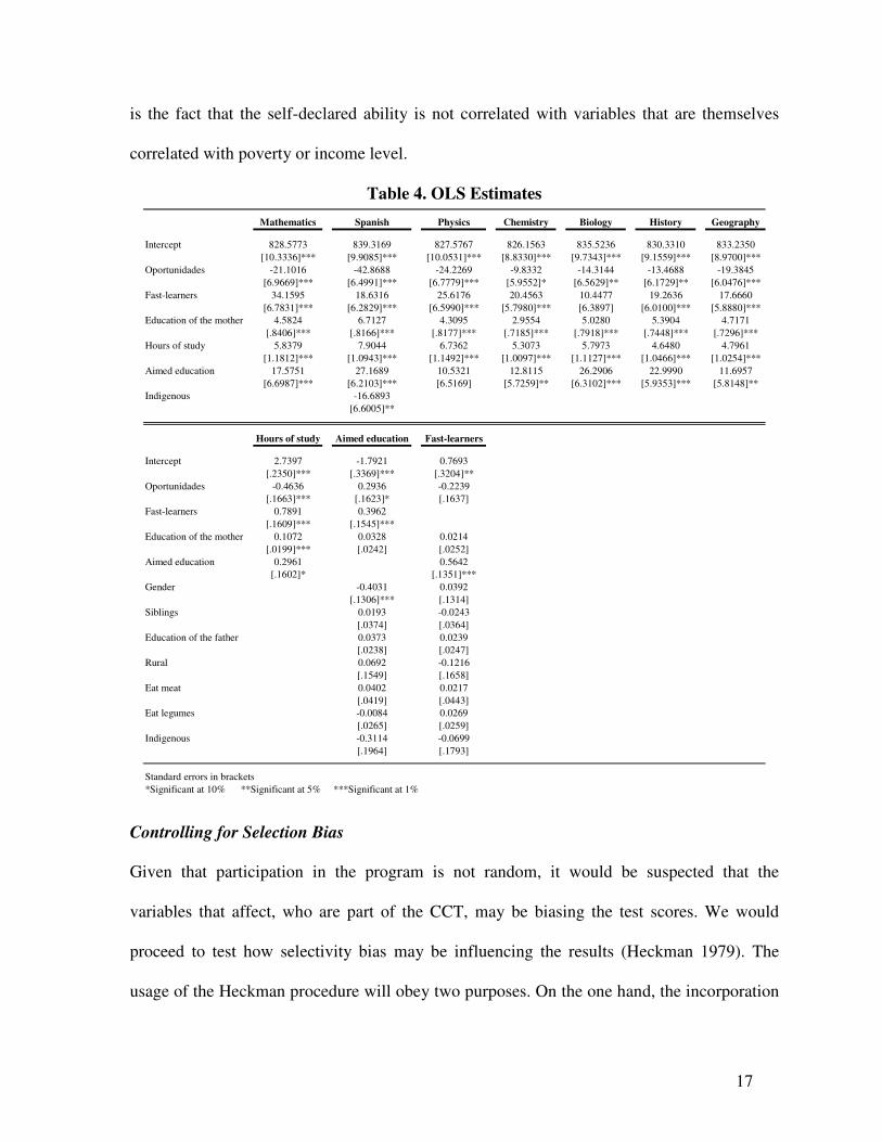
OLS Estimates

A natural benchmark to begin the analysis regards ordinary least squares estimation. The

seven scores of the students were regressed on the following variables: an interceptor,

participation in Oportunidades, a dummy variable with value of one if they considered

themselves fast-learners, the educational level of the mother,9 how many hours they study per

week, and the educational level they aim to complete. In the case of Spanish score, an

explanatory variable was added if the language spoken at home was indigenous.10

Table 4 summarizes our findings. It is worth to note that participation in

Oportunidades is negatively correlated and significant with the seven scores, and the effect is

very big for the Spanish score. With respect to the ability to learn fast, it has a considerable

effect in all the scores. The same can be said for the mother’s education, given the variable

range, for mothers with high levels of education, this variable ends explaining an important

part of the score. Hours devoted to study and the educational level that students want to reach

also have significant effects.

9 63 students reported not living with their mother, but only eight of them did not report the educational level of the mother. In those cases, the mothers are assumed to have no education. 10 We did not found any statistical evidence that this variable was correlated with the other scores. Also, (and contrary to our suspicion) the dummy variable of being in a “telesecondary” was not statistical or economical significant in explaining the scores.

15

Table 3. Description of the Variables

Variable Description Mean Std. Dev.

Aimed educationDummy. 1 for thos who expect to study for4 or more years.

0.2725 0.4455

Eat legumesNumber of portions of legumes they eat perweek.

3.5007 2.6387

Eat meatNumber of portions of meat they eat perweek.

1.4778 1.4189

Education of the father Years of study of the father. 5.3001 3.1583Education of the mother Years of study of the mother. 4.7033 3.3560

Fast-learnersDummy. 1 for those who considerthemselves as fast-learners.

0.6872 0.4639

Gender Dummy. 1 for males. 0.5195 0.4999Hours of study Hours of study per week. 3.4094 2.3811Income Household montly income in pesos. 2409.87 1806.31

IndigenousDummy. 1 for those who speak anindigenous language at home.

0.3248 0.4686

Rural Dummy. 1 for those who live in rural areas. 0.8406 0.3663

Siblings Number of brothers and sisters. 4.2875 2.1322

StateDummy. 1 for those who live in NuevoLeón.

0.2671 0.4427

Variable Description Mean Std. Dev.

Aimed educationDummy. 1 for thos who expect to study for4 or more years.

0.2950 0.4565

Eat legumesNumber of portions of legumes they eat perweek.

3.5125 2.3416

Eat meatNumber of portions of meat they eat perweek.

2.6619 1.8367

Education of the father Years of study of the father. 8.8807 3.8868Education of the mother Years of study of the mother. 8.6590 4.0202

Fast-learnersDummy. 1 for those who considerthemselves as fast-learners.

0.7845 0.4116

Gender Dummy. 1 for males. 0.4895 0.5004Hours of study Hours of study per week. 4.3954 2.9046Income Household montly income in pesos. 3530.25 3563.45

IndigenousDummy. 1 for those who speak anindigenous language at home.

0.0565 0.2311

Rural Dummy. 1 for those who live in rural areas. 0.5690 0.4957

Siblings Number of brothers and sisters. 2.7128 1.6851

StateDummy. 1 for those who live in NuevoLeón.

0.7761 0.4173

With Oportunidades scholarship (N=745)

Without Oportunidades scholarship (N=478)

A series of auxiliary regressions (also included in Table 4) were performed to

investigate possible correlations among the first set of explanatory variables. In particular, we

16

were interested to see if participation in the CCT may affect behavior or expectations. The

first auxiliary regression was studied hours as a dependent variable, keeping the other five as

explanatory variables. As it is shown in the tables, all the variables were significant.

Indirectly participation in the CCT is affecting (in terms of correlation) the scores since

students in the program study on average half an hour less. Both expectations and ability

have a positive and significant effect on studied hours, thus directly and indirectly affecting

the test scores. The education of the mother is playing a role in explaining the studied hours.

Given that the mean educational level (measured in years) of participants’ and non-

participants’ mothers differ (they are 4.71 and 8.66 respectively) another indirect effect is

present.

Two more auxiliary regressions were performed. Using expectation of completed

grades and self-defined ability as dependent variables (both dummies), we did ML logit

regressions on an extended set of explanatory variables. The results are summarized in Table

3. For the first logit regressions, other than the intercept the significant independent variables

were participation in Oportunidades, gender, and the ability to learn fast. The program and

ability have the positive expected sign, meaning that they would also have a positive indirect

effect in the scores. Being a male has a negative effect on the aspired educational level. This

last effect will contradict the Mexican experience where men have on average studied more

years than women have.

The only significant variable (other than the intercept) explaining the ability to learn

fast is the aimed level of study. On the one hand, it is suspected that the causality runs the

other way, and that the regression is just capturing a correlation. Second and very interesting,

17

is the fact that the self-declared ability is not correlated with variables that are themselves

correlated with poverty or income level.

Table 4. OLS Estimates

Mathematics Spanish Physics Chemistry Biology History Geography

Intercept 828.5773 839.3169 827.5767 826.1563 835.5236 830.3310 833.2350[10.3336]*** [9.9085]*** [10.0531]*** [8.8330]*** [9.7343]*** [9.1559]*** [8.9700]***

Oportunidades -21.1016 -42.8688 -24.2269 -9.8332 -14.3144 -13.4688 -19.3845[6.9669]*** [6.4991]*** [6.7779]*** [5.9552]* [6.5629]** [6.1729]** [6.0476]***

Fast-learners 34.1595 18.6316 25.6176 20.4563 10.4477 19.2636 17.6660[6.7831]*** [6.2829]*** [6.5990]*** [5.7980]*** [6.3897] [6.0100]*** [5.8880]***

Education of the mother 4.5824 6.7127 4.3095 2.9554 5.0280 5.3904 4.7171[.8406]*** [.8166]*** [.8177]*** [.7185]*** [.7918]*** [.7448]*** [.7296]***

Hours of study 5.8379 7.9044 6.7362 5.3073 5.7973 4.6480 4.7961[1.1812]*** [1.0943]*** [1.1492]*** [1.0097]*** [1.1127]*** [1.0466]*** [1.0254]***

Aimed education 17.5751 27.1689 10.5321 12.8115 26.2906 22.9990 11.6957[6.6987]*** [6.2103]*** [6.5169] [5.7259]** [6.3102]*** [5.9353]*** [5.8148]**

Indigenous -16.6893[6.6005]**

Hours of study Aimed education Fast-learners

Intercept 2.7397 -1.7921 0.7693[.2350]*** [.3369]*** [.3204]**

Oportunidades -0.4636 0.2936 -0.2239[.1663]*** [.1623]* [.1637]

Fast-learners 0.7891 0.3962[.1609]*** [.1545]***

Education of the mother 0.1072 0.0328 0.0214[.0199]*** [.0242] [.0252]

Aimed education 0.2961 0.5642[.1602]* [.1351]***

Gender -0.4031 0.0392[.1306]*** [.1314]

Siblings 0.0193 -0.0243[.0374] [.0364]

Education of the father 0.0373 0.0239[.0238] [.0247]

Rural 0.0692 -0.1216[.1549] [.1658]

Eat meat 0.0402 0.0217[.0419] [.0443]

Eat legumes -0.0084 0.0269[.0265] [.0259]

Indigenous -0.3114 -0.0699[.1964] [.1793]

*Significant at 10% **Significant at 5% ***Significant at 1% Standard errors in brackets

Controlling for Selection Bias

Given that participation in the program is not random, it would be suspected that the

variables that affect, who are part of the CCT, may be biasing the test scores. We would

proceed to test how selectivity bias may be influencing the results (Heckman 1979). The

usage of the Heckman procedure will obey two purposes. On the one hand, the incorporation

18

of the Inverse Mills ratio (IMR) in the second step will aid in detecting a selection bias and in

its correction. Second, the variables employed in the first step probit can be directly linked to

the model of section II.

The first step probit had participation in Oportunidades as the dependent variable and

the independent ones were an intercept, the number of siblings, the consumption of meat, the

students’ state, and both the mother’s and the father’s education. The obtained coefficients

allowed the calculation of the IMR. The second step consisted in estimating the same

equations used in the OLS models, augmented with the IMR as an extra independent

variable. The results of the second step are summarized in table 4.11 In all the cases, except in

the Spanish equation, the participation in Oportunidades is non-significant. Instead, the IMR

absorbs the effect. To what extent this result suggests the presence of a bias in selection will

be discussed in the analysis section. The effects of three of the explanatory variables (ability,

expected educational level, and hours) remain very stable that is its statistic and economic

significance are unaltered. This is not the case for mother’s education, which is still

significantly correlated with three of the test outcomes (History, Biology, and Spanish), but

whose effects vanish in the other subjects. However, some caution is needed given that the

variable mother’s education is also employed in the first stage. We know that it plays a role

in the selection effect and ultimately in the test scores. Also, and consequently, some

endogeneity is hinted, which will be discussed below.

11 Further information about the first step is available under the request of the reader.

19

Table 5. Controlling for Selection Bias Estimates

Mathematics Spanish Physics Chemistry Biology History Geography

Intercept 811.3910 817.9968 805.2945 819.3079 823.8200 818.2072 820.3474[11.0261]*** [10.6469]*** [10.5867]*** [9.4767]*** [10.4160]*** [9.7116]*** [9.5616]***

Oportunidades -3.5963 -23.3106 -3.4243 -4.7217 -4.0549 -2.7435 -8.2412[7.8671] [7.2666]*** [7.5536] [6.7616] [7.4318] [6.9292] [6.8222]

Fast-learners 33.0893 16.1209 25.3900 20.9796 11.2145 18.5419 18.3167[6.9173]*** [6.3815]** [6.6416]*** [5.9452]*** [6.5345]* [6.0926]*** [5.9985]***

Education of the mother 0.5366 2.2695 -0.4528 1.4753 2.8055 2.2915 1.5255[1.1998] [1.1166]** [1.1520] [1.0312] [1.1334]** [1.0567]** [1.0404]

Hours of study 5.6723 7.7028 6.5701 5.1638 5.7101 4.4391 4.8329[1.1918]*** [1.0997]*** [1.1443]*** [1.0243]*** [1.1259]*** [1.0497]*** [1.0335]***

Aimed education 15.4566 25.9269 7.1677 12.5129 23.7675 21.3644 12.0285[6.7852]** [6.2645]*** [6.5148] [5.8317]** [6.4097]*** [5.9763]*** [5.8839]**

Indigenous -12.3708[6.8165]*

IMR 49.8385 57.0345 58.8615 18.6208 28.8331 37.6853 36.4711[10.3421]*** [9.6269]*** [9.9300]*** [8.8888]** [9.7698]*** [9.1092]*** [8.9684]***

Hours of study Aimed education Fast-learners

Intercept 2.5785 -1.7114 0.6357[.2559]*** [.3432]*** [.3328]*

Oportunidades -0.3089 0.2217 -0.1341[.1899] [.1720] [.1735]

Fast-learners 0.7574 0.4029[.1658]*** [.1548]***

Education of the mother 0.0768 0.0487 0.0026[.0289]*** [.0274]* [.0280]

Aimed education 0.2818 0.4064[.1638]* [.1545]***

Gender -0.4107 0.0467[.1308]*** [.1316]

Siblings 0.0045 -0.0063[.0393] [.0382]

Education of the father 0.0534 0.0048[.0272]** [.0276]

Rural 0.0613 -0.1043[.1551] [.1665]

Eat meat 0.0728 -0.0178[.0497] [.0515]

Eat legumes -0.0042 0.0220[.0267] [.0261]

Indigenous -0.3192 -0.0586[.1964] [.1792]

IMR 0.4322 -0.3776 0.4820[.2497]* [.3077] [.3179]

Standard errors in brackets*Significant at 10% **Significant at 5% ***Significant at 1%

Endogeneity

As commonly happens in economic/social empirical analysis, we suspect that the model

suffers of endogeneity, which means that one or some of the independent variables is (are)

correlated with unobservable variables captured in the error term. This problem leads to

biased parameters. A solution is the use of instrumental variables (IV). We employ

instrumental variables via the Generalized Method of Moments. The chosen instruments

20

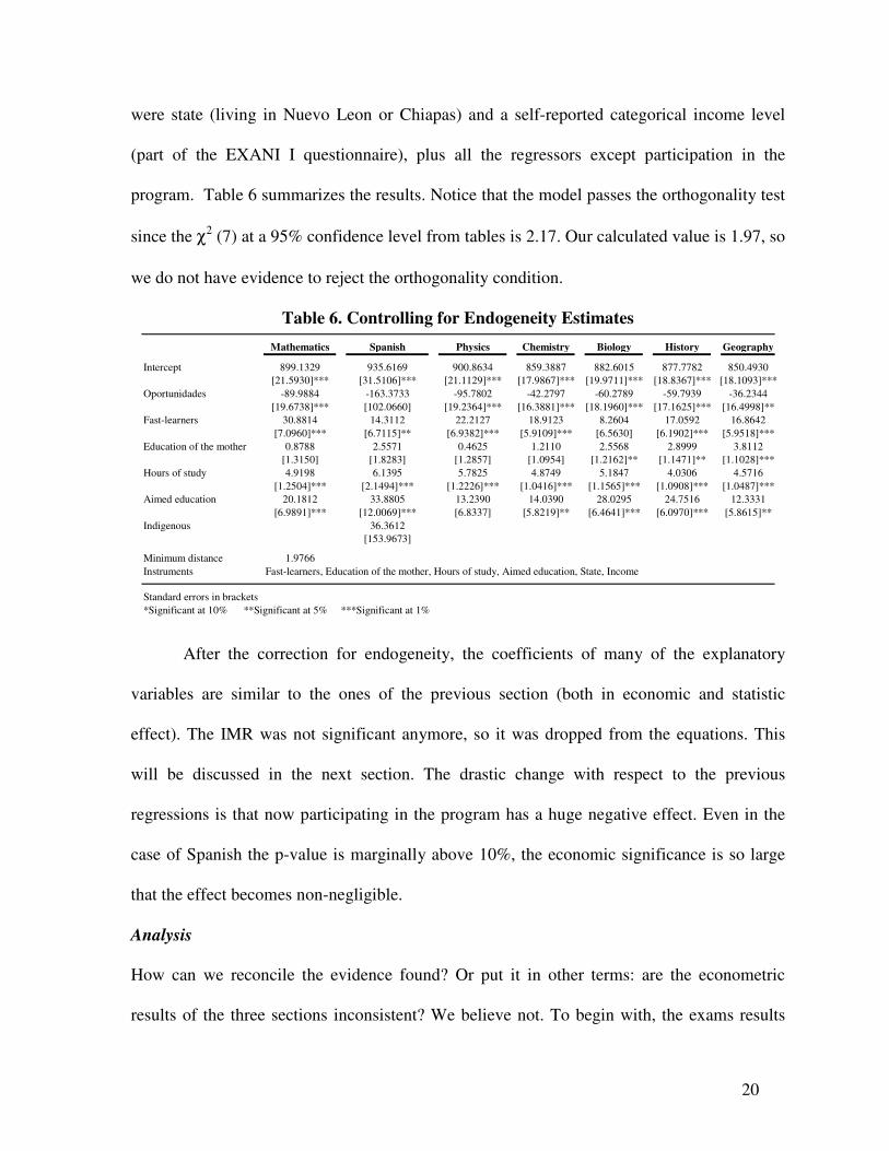
were state (living in Nuevo Leon or Chiapas) and a self-reported categorical income level

(part of the EXANI I questionnaire), plus all the regressors except participation in the

program. Table 6 summarizes the results. Notice that the model passes the orthogonality test

since the χ2 (7) at a 95% confidence level from tables is 2.17. Our calculated value is 1.97, so

we do not have evidence to reject the orthogonality condition.

Table 6. Controlling for Endogeneity Estimates

Mathematics Spanish Physics Chemistry Biology History Geography

Intercept 899.1329 935.6169 900.8634 859.3887 882.6015 877.7782 850.4930[21.5930]*** [31.5106]*** [21.1129]*** [17.9867]*** [19.9711]*** [18.8367]*** [18.1093]***

Oportunidades -89.9884 -163.3733 -95.7802 -42.2797 -60.2789 -59.7939 -36.2344[19.6738]*** [102.0660] [19.2364]*** [16.3881]*** [18.1960]*** [17.1625]*** [16.4998]**

Fast-learners 30.8814 14.3112 22.2127 18.9123 8.2604 17.0592 16.8642[7.0960]*** [6.7115]** [6.9382]*** [5.9109]*** [6.5630] [6.1902]*** [5.9518]***

Education of the mother 0.8788 2.5571 0.4625 1.2110 2.5568 2.8999 3.8112[1.3150] [1.8283] [1.2857] [1.0954] [1.2162]** [1.1471]** [1.1028]***

Hours of study 4.9198 6.1395 5.7825 4.8749 5.1847 4.0306 4.5716[1.2504]*** [2.1494]*** [1.2226]*** [1.0416]*** [1.1565]*** [1.0908]*** [1.0487]***

Aimed education 20.1812 33.8805 13.2390 14.0390 28.0295 24.7516 12.3331[6.9891]*** [12.0069]*** [6.8337] [5.8219]** [6.4641]*** [6.0970]*** [5.8615]**

Indigenous 36.3612[153.9673]

Minimum distance 1.9766Instruments Fast-learners, Education of the mother, Hours of study, Aimed education, State, Income

Standard errors in brackets*Significant at 10% **Significant at 5% ***Significant at 1%

After the correction for endogeneity, the coefficients of many of the explanatory

variables are similar to the ones of the previous section (both in economic and statistic

effect). The IMR was not significant anymore, so it was dropped from the equations. This

will be discussed in the next section. The drastic change with respect to the previous

regressions is that now participating in the program has a huge negative effect. Even in the

case of Spanish the p-value is marginally above 10%, the economic significance is so large

that the effect becomes non-negligible.

Analysis

How can we reconcile the evidence found? Or put it in other terms: are the econometric

results of the three sections inconsistent? We believe not. To begin with, the exams results

21

summarized in Table 2 suggest that participants in the program do have lower scores than

non-participants. These results were aligned with the predictions of the theoretical model of

section II. The negative correlation between the CCT participation and scores were backed

up by each of the econometric specifications, but in different ways. OLS regressions show

that there exists the negative correlation but that other variables are playing a role too.

Moreover, participation in the program may have indirect effects since it is correlated itself

with the other variables.

When selection bias correction is introduced via the IMR, the significance of

participating in the program vanishes. These results are consistent with the theoretical model:

it is not that participation in CCT lower grades, but participants in the program are expected

to have a poorer performance because of the incomplete homologation and the switching

effect. Thus, selectivity bias seems important.

With the suspicion of endogeneity, participation in the program is instrumented via a

self-reported income level and state of residence (with the two states in our sample showing

very different standards of living). Again, participation is the program is highly negative

correlated with test scores. While the effects of the other explanatory variables remains

qualitatively very similar.

To understand why a negative correlation is showing up, we rely again in the

theoretical model. We found some evidence that supports the switching effect: participants in

the program study less hours, have lower future schooling expectations, and define

themselves as slightly less able. Nonetheless, the major part of the difference in scores

appears to be caused by variables (observed and unobserved) associated to living standards.

In terms of our model, while the cash transfers may cause an immediate relief, they may not

22

solve other problems (e.g. attending quality schools, living in good neighborhoods, etc.).

Thus an incomplete homologation between participants and non-participants may be

occurring.

V. Conclusions

Conditional Cash Transfers (CCT) appear nowadays as the silver bullets of social policy:

constantly more governments are interested in implementing them. The rationale behind this

behavior seems understandable: in general, the assessments of existing CCT show that they

have been effective. In the particular case of education, it seems that targeted CCT are very

good to improve enrollment.

In this paper, we argue that while the quantity effect in education (enrollment) has

been studied with some detail, much fewer has been written about the quality effect. A

theoretical model is presented with some pessimistic predictions: it is expected that

participants in CCT should have lower grades. The result is caused by two effects: a

switching effect (similar in logic to revealed preference) where some students may decide to

switch because of the CCT and will do the minimum to remain in track. Secondly, while the

transfer component of the program may cause relief, an incomplete homologation would

appear because the program is not able to provide conditions experienced by less poor

students (better educated parents, access to services, good neighborhoods, higher quality

schools, etc.).

A dataset that includes participants and non-participants in a famous Mexican CCT

(i.e. Progresa/Oportunidades), students’ test scores, plus a series of sociodemographic

variables allows us to test different econometric specifications. Participants in the CCT do

23

have lower test scores. While we found some evidence of a switching effect, most of the

difference appears related to the incomplete homologation.

CCT are expected to promote the accumulation of human capital. Past studies and

assessments suggest that they are effective, but the quality component is often not

considered. This paper points that “leveling the field” between poor students and others

better off may be harder than expected. That is, while cash transfers may help, there are other

variables to consider if schooling quality is to be equated. Future research on the

determinants of school grades and public policies to enhance them should prove

instrumental.

Bibl iography

Alderman, Harold, Jere R. Behrman, Shahrukh Khan, David R. Ross, and Richard Sabot. “The Income Gap in Cognitive Skills in Rural Pakistan.” Journal of Economic Development and Cultural Change 46, no. 1 (1997) : 97-122.

Behrman, Jere R., Piyali Sengupta, and Petra Todd. The Impact of Progresa on

Achievement Test Scores in the First Year. Washington, D.C.: International Food Policy Research Institute, 2000.

________. “Progressing through PROGRESA: An Impact Assessment of a School

Subsidy Experiment in Rural Mexico.” Journal of Economic Development and Cultural Change Vol. 54, no. 1 (2005) : 237.

Behrman, Jere R., Susan W. Parker, and Petra E. Todd. Technical Documents on the

Evaluation of Oportunidades. Vol. 9, Medium-Term Effects of the Oportunidades

Program Package, including Nutrition, on Education of Rural Children Age 0-8

in 1997. Mexico : Instituto Nacional de Salud Pública, 2004. Black, Sandra E., Paul J. Deveraux, and Kjell G. Salvanes. “The More the Merrier? The

effect of Family Composition on Children’s Education.” NBER Working Paper Series, no. 10720 (2004) : 1-48.

Borland, Melvin V., and Roy M. Howsen. “A Note on Student Academic Performance In

Rural Versus Urban Areas.” American Journal of Economics and Sociology 58, no. 3 (1999) : 538-546.

24

Bourguignon, François, Francisco H. G. Ferreria, and Phillippe G. Leite. “Conditional Cash Transfers, Schooling, and Child Labor: Micro-Simulating Brazil’s Bolsa Esola Program.” The World Bank Economic Review Vol. 17, no. 2 (2003) : 229.

Brown, Philip H. and Albert Park. “Education and Poverty in Rural China.” Economics

of Education Review Vol. 21 (2002) : 523-541. Browning, Martin, Pierre-André Chiappori, and Arthur Lewbel. “Estimating Consumption Economies of Scale, Adult Equivalent Scales, and Household Bargaining Power.” CAM Working Paper (2005) : 1-46. Das, Jishnu, Quy-Toan Do, and Berk Özler. “Conditional Cash Transfers and the Equity-

Efficiency Debate.” World Bank Policy Research Working Paper, no. 3280 (2004) : 1-29. Available at http://ssrn.com/abstract=610325

________. “Reassessing Conditional Cash Transfer Programs.” World Bank Research

Observer Vol. 20, no. 1 (2005) : 57-80. Available at http://ssrn.com/ abstract=873739

De Fraja, Gianni, Tania Oliveira, and Luisa Zanchi . “Must Try Harder. Evaluating the

Role of Effort in Educational Attainment.” Centre for Economic Policy Research Discussion Paper, no. 5048 (2005) : 1-30.

Dooley, Martin, and Jennifer Stewart. “Family income and child outcomes in Canada.”

Canadian Journal of Economics 37, no. 4 (2004) : 899-917. Gertler, Paul J. and Lia C. Fernald. “Impacto de mediano plazo del Programa Oportunidades sobre el desarrollo infantil en áreas rurales.” (2005) Heckman, James J. “Sample Selection Bias as a Specification Error.” Econometrita Vol.

47, no. 1 (1979) : 153-162. Kreps, David M. A Course in Microeconomic Theory. Princeton, New Jersey: Princeton

University Press, 1990. Lindert, Kathy, Emmanuel Skoufias, and Joseph Shapiro. “Redistribution of Income to

the Poor and the Rich: Public Transfers in Latin America and the Caribbean.” The World Bank (2005) : 1-123.

McEwan, Patrick J. “The Indigenous Test Score Gap in Bolivia and Chile.” Journal

of Economic Development and Cultural Change (2004) : 157-190. McNabb, Robert, Saramistha Pal, and Peter Sloane. “Gender Differences in Educational

Attainment: The Case of University Students in England and Wales.” Economica 69 (2002) : 481-503.

25

Parker, Susan W., Petra E. Todd, and Kenneth I. Wolpin. “Within-Family Treatment

Effect Estimators: The Impact of Oportunidades on Schooling in Mexico.” Unpublished manuscript.

Paxson, Christina, and Norbert Schady. “Cognitive Development Among Young

Children in Ecuador: The Roles of Wealth, Health and Parenting.” World Bank Policy Research Working Paper, no. 3605 (2005) : 1-32.

Rawlings, Laura B. and Gloria Rubio. “Evaluating the Impact of Conditional Cash

Transfer Programs. Lessons from America Latina.” Policy Research Working Paper, no. 3119 (2003): 1-29.

Shultz, T. Paul. Impact of Progresa on School Attendance Rates in the Sampled

Population. Washington, D.C.: International Food Policy Research Institute, 2000.

Skoufias, Emmanuel, and Susan Parker. “Conditional Cash Transfers and Their Impact on Child Work and Schooling: Evidence from the Progresa Program in Mexico.” FCND Discussion Paper, no. 123 (2001) : 1-61.

Varian, Hal R. Microeconomic Analysis. 3rd ed. New York: W. W. Norton & Company,

Inc., 1992.