Do Asian investors rebalance their portfolios and … Asian investors rebalance their portfolios and...
31
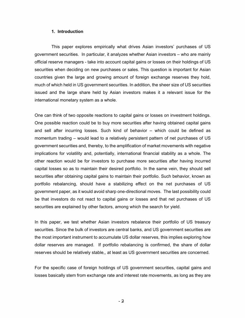
Do Asian investors rebalance their portfolios and what are the consequences? Alicia García-Herrero 1 and Akiko Terada-Hagiwara 2 3 October 2006 Abstract This paper explores empirically whether Asian investors, and in particular foreign reserve managers, respond to capital gains or losses by rebalancing their portfolios of US Treasury securities. For a sample of 10 Asian countries from 1990 to end 2004, we find that capital losses —stemming from dollar depreciation against the euro or lower returns on US Treasury securities —increase the net purchases of such securities. The fact that Asian investors appear to rebalance their portfolios should reduce the likelihood of one-directional movements in the net purchases of US securities. Given the sheer size of the US fiscal deficit, much of which financed by Asian investors, this should have contributed to limiting the volatility of the international monetary system. Key words: portfolio rebalancing, reserve management, Asia JEL classification: E44, E58, F31 1 Alicia Garcia-Herrero is affiliated with the BIS Regional Office for Asia and the Pacific. She can be contacted at [email protected]. 2 Akiko Terada-Hagiwara is affiliated with the Bank of Japan. She can be contacted at [email protected]. 3 Views expressed in this paper are those of the authors and do not necessarily reflect the official views of the Bank of Japan or the BIS. Useful comments have been received from Claudio Borio, Andrew Filardo, Jacob Gyntelberg, Kentaro Kawasaki, Bob McCauley, Frank Packer, Eli Remolona, Daniel Santabarbara, Francisco Vazquez, Eliza Wu and participants to the International Conference on Financial System Reform and Monetary Policies in Asia, hosted by Hitotsubashi University (September 15-16, 2006). We also appreciate excellent research assistance by Eric Chan. Remaining errors are obviously the authors’. - - 1
Transcript of Do Asian investors rebalance their portfolios and … Asian investors rebalance their portfolios and...
Do Asian investors rebalance their portfolios and what are the consequences?
Alicia García-Herrero1 and Akiko Terada-Hagiwara2 3 October 2006
Abstract
This paper explores empirically whether Asian investors, and in particular foreign reserve
managers, respond to capital gains or losses by rebalancing their portfolios of US Treasury
securities. For a sample of 10 Asian countries from 1990 to end 2004, we find that capital
losses —stemming from dollar depreciation against the euro or lower returns on US
Treasury securities —increase the net purchases of such securities. The fact that Asian
investors appear to rebalance their portfolios should reduce the likelihood of one-directional
movements in the net purchases of US securities. Given the sheer size of the US fiscal
deficit, much of which financed by Asian investors, this should have contributed to limiting
the volatility of the international monetary system.
Key words: portfolio rebalancing, reserve management, Asia
JEL classification: E44, E58, F31
1 Alicia Garcia-Herrero is affiliated with the BIS Regional Office for Asia and the Pacific. She can be contacted at [email protected]. 2 Akiko Terada-Hagiwara is affiliated with the Bank of Japan. She can be contacted at [email protected]. 3 Views expressed in this paper are those of the authors and do not necessarily reflect the official views of the Bank of Japan or the BIS. Useful comments have been received from Claudio Borio, Andrew Filardo, Jacob Gyntelberg, Kentaro Kawasaki, Bob McCauley, Frank Packer, Eli Remolona, Daniel Santabarbara, Francisco Vazquez, Eliza Wu and participants to the International Conference on Financial System Reform and Monetary Policies in Asia, hosted by Hitotsubashi University (September 15-16, 2006). We also appreciate excellent research assistance by Eric Chan. Remaining errors are obviously the authors’.
- - 1
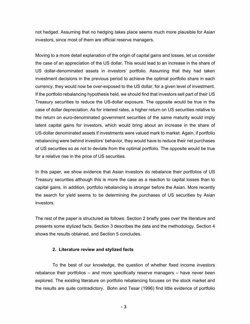
1. Introduction
This paper explores empirically what drives Asian investors’ purchases of US
government securities. In particular, it analyzes whether Asian investors – who are mainly
official reserve managers - take into account capital gains or losses on their holdings of US
securities when deciding on new purchases or sales. This question is important for Asian
countries given the large and growing amount of foreign exchange reserves they hold,
much of which held in US government securities. In addition, the sheer size of US securities
issued and the large share held by Asian investors makes it a relevant issue for the
international monetary system as a whole.
One can think of two opposite reactions to capital gains or losses on investment holdings.
One possible reaction could be to buy more securities after having obtained capital gains
and sell after incurring losses. Such kind of behavior – which could be defined as
momentum trading – would lead to a relatively persistent pattern of net purchases of US
government securities and, thereby, to the amplification of market movements with negative
implications for volatility and, potentially, international financial stability as a whole. The
other reaction would be for investors to purchase more securities after having incurred
capital losses so as to maintain their desired portfolio. In the same vein, they should sell
securities after obtaining capital gains to maintain their portfolio. Such behavior, known as
portfolio rebalancing, should have a stabilizing effect on the net purchases of US
government paper, as it would avoid sharp one-directional moves. The last possibility could
be that investors do not react to capital gains or losses and that net purchases of US
securities are explained by other factors, among which the search for yield.
In this paper, we test whether Asian investors rebalance their portfolio of US treasury
securities. Since the bulk of investors are central banks, and US government securities are
the most important instrument to accumulate US dollar reserves, this implies exploring how
dollar reserves are managed. If portfolio rebalancing is confirmed, the share of dollar
reserves should be relatively stable,, at least as US government securities are concerned.
For the specific case of foreign holdings of US government securities, capital gains and
losses basically stem from exchange rate and interest rate movements, as long as they are
- - 2
not hedged. Assuming that no hedging takes place seems much more plausible for Asian
investors, since most of them are official reserve managers.
Moving to a more detail explanation of the origin of capital gains and losses, let us consider
the case of an appreciation of the US dollar. This would lead to an increase in the share of
US dollar-denominated assets in investors’ portfolio. Assuming that they had taken
investment decisions in the previous period to achieve the optimal portfolio share in each
currency, they would now be over-exposed to the US dollar, for a given level of investment.
If the portfolio rebalancing hypothesis held, we should find that investors sell part of their US
Treasury securities to reduce the US-dollar exposure. The opposite would be true in the
case of dollar depreciation. As for interest rates, a higher return on US securities relative to
the return on euro-denominated government securities of the same maturity would imply
latent capital gains for investors, which would bring about an increase in the share of
US-dollar denominated assets if investments were valued mark to market. Again, if portfolio
rebalancing were behind investors’ behavior, they would have to reduce their net purchases
of US securities so as not to deviate from the optimal portfolio. The opposite would be true
for a relative rise in the price of US securities.
In this paper, we show evidence that Asian investors do rebalance their portfolios of US
Treasury securities although this is more the case as a reaction to capital losses than to
capital gains. In addition, portfolio rebalancing is stronger before the Asian. More recently
the search for yield seems to be determining the purchases of US securities by Asian
investors.
The rest of the paper is structured as follows: Section 2 briefly goes over the literature and
presents some stylized facts. Section 3 describes the data and the methodology. Section 4
shows the results obtained, and Section 5 concludes.
2. Literature review and stylized facts
To the best of our knowledge, the question of whether fixed income investors
rebalance their portfolios – and more specifically reserve managers – have never been
explored. The existing literature on portfolio rebalancing focuses on the stock market and
the results are quite contradictory. Bohn and Tesar (1996) find little evidence of portfolio
- - 3
rebalancing by foreign investors in the US equity market. Hau and Rey (2004), instead,
show that international equity returns, equity portfolio flows and exchange rate returns can
be explained by portfolio rebalancing after controlling for endogeneity.
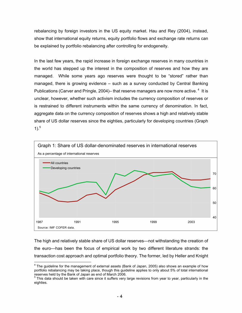
In the last few years, the rapid increase in foreign exchange reserves in many countries in
the world has stepped up the interest in the composition of reserves and how they are
managed. While some years ago reserves were thought to be “stored” rather than
managed, there is growing evidence – such as a survey conducted by Central Banking
Publications (Carver and Pringle, 2004)– that reserve managers are now more active. 4 It is
unclear, however, whether such activism includes the currency composition of reserves or
is restrained to different instruments within the same currency of denomination. In fact,
aggregate data on the currency composition of reserves shows a high and relatively stable
share of US dollar reserves since the eighties, particularly for developing countries (Graph
1).5
- - 4
Graph 1: Share of US dollar-denominated reserves in international reserves As a percentage of international reserves
40
50
60
70
1987 1991 1995 1999 2003
All countriesDeveloping countries
Source: IMF COFER data.
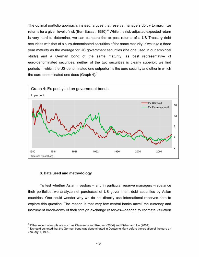
The high and relatively stable share of US dollar reserves—not withstanding the creation of
the euro—has been the focus of empirical work by two different literature strands: the
transaction cost approach and optimal portfolio theory. The former, led by Heller and Knight
4 The guideline for the management of external assets (Bank of Japan, 2005) also shows an example of how portfolio rebalancing may be taking place, though this guideline applies to only about 5% of total international reserves held by the Bank of Japan as end of March 2006. 5 This data should be taken with care since it suffers very large revisions from year to year, particularly in the eighties.
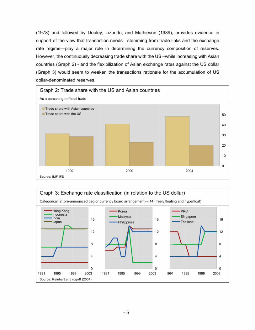
(1978) and followed by Dooley, Lizondo, and Mathieson (1989), provides evidence in
support of the view that transaction needs—stemming from trade links and the exchange
rate regime—play a major role in determining the currency composition of reserves.
However, the continuously decreasing trade share with the US –while increasing with Asian
countries (Graph 2) - and the flexibilization of Asian exchange rates against the US dollar
(Graph 3) would seem to weaken the transactions rationale for the accumulation of US
dollar-denominated reserves.
- - 5
Graph 3: Exchange rate classification (in relation to the US dollar) Categorical: 2 (pre-announced peg or currency board arrangement) – 14 (freely floating and hyperfloat)
Source: Reinhart and rogoff (2004)
Graph 2: Trade share with the US and Asian countries As a percentage of total trade
0
10
20
30
40
50
1990 2000 2004
Trade share with Asian countriesTrade share with the US
Source: IMF IFS
0
4
8
12
16
1991 1995 1999 2003
Hong KongIndonesiaIndiaJapan
0
4
8
12
16
1991 1995 1999 2003
KoreaMalaysiaPhilippines
0
4
8
12
16
1991 1995 1999 2003
PRCSingaporeThailand
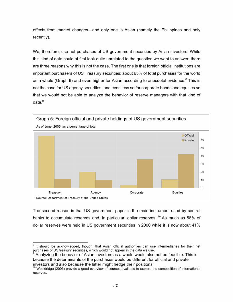
The optimal portfolio approach, instead, argues that reserve managers do try to maximize
returns for a given level of risk (Ben-Bassat, 1980).6 While the risk-adjusted expected return
is very hard to determine, we can compare the ex-post returns of a US Treasury debt
securities with that of a euro-denominated securities of the same maturity. If we take a three
year maturity as the average for US government securities (the one used in our empirical
study) and a German bond of the same maturity, as best representative of
euro-denominated securities, neither of the two securities is clearly superior: we find
periods in which the US-denominated one outperforms the euro security and other in which
the euro-denominated one does (Graph 4).7
- - 6
Graph 4: Ex-post yield on government bonds In per cent
0
4
8
12
16
1980 1984 1988 1992 1996 2000 2004
2Y US yield2Y Germany yield
Source: Bloomberg
3. Data used and methodology
To test whether Asian investors – and in particular reserve managers –rebalance
their portfolios, we analyze net purchases of US government debt securities by Asian
countries. One could wonder why we do not directly use international reserves data to
explore this question. The reason is that very few central banks unveil the currency and
instrument break-down of their foreign exchange reserves—needed to estimate valuation
6 Other recent attempts are such as Claessens and Kreuser (2004) and Fisher and Lie (2004). 7 It should be noted that the German bond was denominated in Deutsche Mark before the creation of the euro on January 1, 1999.
effects from market changes—and only one is Asian (namely the Philippines and only
recently).
We, therefore, use net purchases of US government securities by Asian investors. While
this kind of data could at first look quite unrelated to the question we want to answer, there
are three reasons why this is not the case. The first one is that foreign official institutions are
important purchasers of US Treasury securities: about 65% of total purchases for the world
as a whole (Graph 6) and even higher for Asian according to anecdotal evidence.8 This is
not the case for US agency securities, and even less so for corporate bonds and equities so
that we would not be able to analyze the behavior of reserve managers with that kind of
data.9
- - 7
Graph 5: Foreign official and private holdings of US government securities As of June, 2005, as a percentage of total
0
10
20
30
40
50
60
Treasury Agency Corporate Equities
OfficialPrivate
Source: Department of Treasury of the United States
The second reason is that US government paper is the main instrument used by central
banks to accumulate reserves and, in particular, dollar reserves. 10 As much as 58% of
dollar reserves were held in US government securities in 2000 while it is now about 41%
8 It should be acknowledged, though, that Asian official authorities can use intermediaries for their net purchases of US treasury securities, which would not appear in the data we use. 9 Analyzing the behavior of Asian investors as a whole would also not be feasible. This is because the determinants of the purchases would be different for official and private investors and also because the latter might hedge their positions. 10 Wooldridge (2006) provide a good overview of sources available to explore the composition of international reserves.
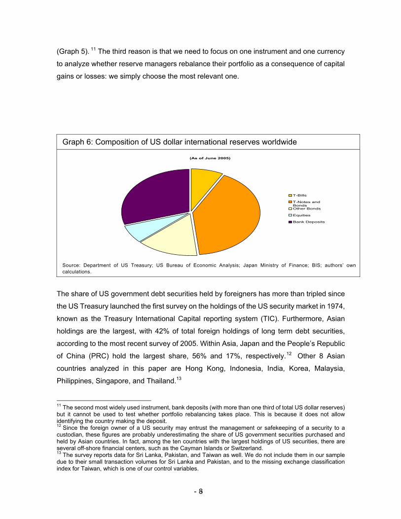
(Graph 5). 11 The third reason is that we need to focus on one instrument and one currency
to analyze whether reserve managers rebalance their portfolio as a consequence of capital
gains or losses: we simply choose the most relevant one.
Graph 6: Composition of US dollar international reserves worldwide
(As of June 2005)
T-Bills
T-Notes andBondsOther Bonds
Equities
Bank Deposits
Source: Department of US Treasury; US Bureau of Economic Analysis; Japan Ministry of Finance; BIS; authors’ own calculations.
The share of US government debt securities held by foreigners has more than tripled since
the US Treasury launched the first survey on the holdings of the US security market in 1974,
known as the Treasury International Capital reporting system (TIC). Furthermore, Asian
holdings are the largest, with 42% of total foreign holdings of long term debt securities,
according to the most recent survey of 2005. Within Asia, Japan and the People’s Republic
of China (PRC) hold the largest share, 56% and 17%, respectively.12 Other 8 Asian
countries analyzed in this paper are Hong Kong, Indonesia, India, Korea, Malaysia,
Philippines, Singapore, and Thailand.13
11 The second most widely used instrument, bank deposits (with more than one third of total US dollar reserves) but it cannot be used to test whether portfolio rebalancing takes place. This is because it does not allow identifying the country making the deposit. 12 Since the foreign owner of a US security may entrust the management or safekeeping of a security to a custodian, these figures are probably underestimating the share of US government securities purchased and held by Asian countries. In fact, among the ten countries with the largest holdings of US securities, there are several off-shore financial centers, such as the Cayman Islands or Switzerland. 13 The survey reports data for Sri Lanka, Pakistan, and Taiwan as well. We do not include them in our sample due to their small transaction volumes for Sri Lanka and Pakistan, and to the missing exchange classification index for Taiwan, which is one of our control variables.
- - 8
The TIC survey offers a breakdown of monthly net purchases of US government debt
securities into less than one year (T-bills) and more than one year (T-notes and bonds), and
reports that the maturity structure of this latter group concentrates between 1-5 years
making up more than 50% of total. On the private versus official nature of the foreign
holders of US government securities, only aggregate information exists but not country by
country. However, as has already been mentioned, it can safely be argued that a very large
share of the Asian holdings of US long-term government securities is in official hands. This
is even more so the case since capital controls on outflows, though varying in degrees,
have been in place in most of our sample countries except for financially developed
countries, such as Hong Kong, Japan, and Singapore.
In order to explore whether portfolio rebalancing affects Asian’s net purchases of US
long-term government debt securities, we follow Bohn and Tesar (1996)’s set out. They
show that net purchases of a certain asset can be decomposed in two determining factors;
one that arises from a change in the desired portfolio and the other that stems from capital
gains or losses on the total portfolio and on the US Treasury securities as follows.14
)()()( 1,1,,,1,1,,, −−−− −+−= titiustitititititi WxccWxxNP (1)
where be the net purchases of US government securities by an Asian country i at time
t. stands for the portfolio share of total wealth (W ) allocated to US government
securities. W is proxied with the stock of exchange rate reserves, as most of the investors
are official institutions. c and stand for capital gains on the total portfolio and capital
gains on the US dollar denominated securities, respectively, both expressed in US dollar
terms.
itNP
itx 1, −ti
it
ti,ustic ,
In order to calculate capital gains and losses on the US government securities held by Asian
countries, we need to think of the available choice for an average reserve manager at an
Asian official institution. For simplicity, we assume that he can only choose between US
14 This setout is approximated from the fact that NP can be written as
, and W is a function of the return on the total portfolio between
t-1 and t (Bohn and Tesar (1996)).
it
)Wx)(c1(WxNP 1t,i1t,iusitt,it,it,i −−+−= it
- - 9
dollar or euro assets. This means that capital gains or losses can stem from changes in the
dollar euro exchange rate, as well as price changes in US government securities relative to
those in euro-denominated securities of the same maturity, liquidity and credit risk. The
capital gains on the total portfolio c can, then, be written as follows. t,i
ust,iti
et,itit,i cxc)x1(c
t,t,+−= (2)
By replacing in equation (1) with equation (2), can be written as follows: t,ic itNP
)Wx)(x1()cc(W)xx(NP 1t,i1t,i1t,iet,i
ust,i1t,i1t,it,it,i −−−−− −−+−= (3)
where stands for the relative capital gains on that portfolio as compared to one
of a similar maturity, risk and liquidity but denominated in euros.
)( ,,eti
usti cc −
Given the fact that the holdings of long-term US government securities are very
concentrated on the 1-5 year maturity, we assume that their average remaining maturity to
be 3 years.15 We, thus, take the price of a three-year US government bond and that of a
three year German bond to calculate interest-rate related capital gains or losses.16 We can
quite safely assume that liquidity and credit risk are the same. Capital gains on US
securities relative to those on euro will, then, be defined in the following way:
=− euit
usit cc +{( )- } (4) )/ln( 1−tt ee $
1$
−− tt rr )( 1et
et rr −−
where stands for euro exchange rate vis-à-vis US dollar (i.e., an increase in implies a
dollar appreciation), r and stand for returns on the US government securities and on
German government securities of a three-year maturity.
te te
$t
etr
As for the first term of equation (3), the question is how the share of securities, x , is
chosen. We test the two major explanations offered by the literature: the transaction costs
and the portfolio optimization. The former implies that trade with the US, borrowing in US
dollar or an exchange rate regime linked to the dollar should increase the demand for US
dollar reserves and, thereby, for US government securities. Since we are trying to explain a
flow variable (net purchases of US paper and not the outstanding stock), we test whether
changes in transaction costs affect the currency breakdown of reserves by increasing or
it
15 Robustness tests are conducted with other maturities, such as two and five years. Three years is preferred because the two-year period could be more influenced by monetary policy expectations and the five year period is too long an average maturity for our sample. 16A German bond was chosen since it is more similar to a US treasury in terms of liquidity and risk.
- - 10
decreasing such net purchases. Two variables stand for the transaction costs: Trade and
. The former is proxied by the sum of imports and exports to the US as percentage of
each Asian country’s total imports and exports. The latter measures the degree of flexibility
of the exchange rate regime using the de-facto exchange rate classification constructed by
Reinhart and Rogoff (2004). This is a categorical variable, which goes from 2 to 14; the
higher number indicates a more flexible exchange rate. A priori is that the fixer the regime
against the dollar, the larger the need for US dollar denominated reserves for intervention
purposes. The amount of debt in US dollar could not be included due to the low frequency of
the data (annual, if available).
t,i
r(sd/r tet
t,iExch
=it fx
As for the hypothesis that reserves are managed according to optimal portfolio theory, we
assume that the degree of risk aversion is fixed, and the variance-covariance matrix of
returns is constant. These assumptions allow us to focus on a change in returns as a factor
affecting the portfolio weight adjustment. To that end, we include an additional term in the
equation measuring the expected risk-adjusted rate of return of US government securities
relative to euro-denominated ones. We measure the risk-adjusted return with the Sharpe
ratio (average yield divided by the standard deviation, )
and assume today’s value to be the best forecast of tomorrow’s risk-adjusted return (i.e., a
random walk). Since we assume that investors choose their preferred portfolio based on
the transaction costs and the risk-adjusted profitability of the previous period, the preferred
share of US treasury securities, , is a linear function of the three variables as follows.
))r(sd/rSharpe eust
ustt −=
itx
),,( 11,1, −−− ttiti SharpeExchTrade (5)
That preferred portfolio is, then, affected by exchange rate and interest rate developments,
which lead to capital gains or losses. Such capital gains and losses stemming from the
previous period may affect investors’ net purchases of US government securities today.
The process is then repeated and investors recalculate their preferred portfolio on the basis
of changes in transaction costs and risk-adjusted profitability. In other words, the
determinants of the optimal portfolio entered the equation explaining net purchases of US
- - 11
securities with one lag while the portfolio rebalancing hypothesis enters
contemporaneously.17
We replace the first term of equation (3) with equation (5), and divide by investors’ total
wealth in the previous period, W 1, −ti18, we obtain the following estimating equation:
1t41t,i31t,i21t,i1t,ieuit
usit1
1t,i
it SharpeExchTradex)x1)(cc(WNP
−−−−−−
+++−−= ββββ + itε (6)
where stands for the relative capital gain as defined in equation (4); Trade
refers to a change in trade share with US in the previous period; TR ,
stands for a change in the de facto exchange rate regime in the previous period,
; and represents the change in the risk-adjusted return on of a
two-year US government security as compared to a German one of the same maturity.
euit
usit cc −
2t,iE −
1t,i −
1t,iExch −2t,i1t,i TR −− −
1t,iE − −
it
1tSharpe −
19
ε is the error term.
Equation (6) shows the two previously mentioned components to an investors’ decision to
purchase US government securities. The first term is the portfolio rebalancing effect given
the preferred share determined in the previous period, . If capital gains on the share of
US government securities are larger than that on euro-denominated assets, i.e., if
are positive, the investor should sell off some of his/her outstanding US
government securities to approach his/her desired portfolio. The opposite would be true if
the relative capital gains ( are negative. The second component indicates that net
purchases will be positive if the investor’s desired weight of that specific
currency/instrument increases between period t-1 and t.
1itx −
)( ,,eti
usti cc −
),,eti
usti cc −
17In theory, this should be a continuous-time problem but it can be safely assumed that investors –and in particular reserve managers – take decisions with a certain frequency. 18 The fact that we divide by W also implies that we are controlling for trends in the total amount of reserves. In other words, the accumulation of reserves is treated as exogenous and controlled for. This is because the paper aims at understanding investment decisions across instruments and currencies and not at explaining the level of reserves. In addition, taking wealth one period before allows our dependent variable not to be influenced by the evolution of exchange and interest rates between t-1 and t.
1, −ti
19 Further details can be found in Table A1 in the Appendix.
- - 12
Finally, separating the relative capital gains in the exchange rate and the return component
as in (4), we would have the following estimation equation:
itttiti
titiet
et
ust
usttiti
ti
it
SharpeExchTrade
xxrrrrxxWNP
ηγγγ
γγ
++++
−−+−+−=
−−−
−−−−−−−
151,41,3
1,1,1121,1,1-tt11,
)1()}(){()1() /eeln( (7)
We have monthly panel data for 10 countries for the period 1990 to 2004. This amounts to
1514 observations. The monthly frequency tries to strike a balance between the transaction
cost-related reasons to accumulate reserves and the others (portfolio rebalancing and
search for yield). The latter are probably a high frequency event as compared with the share
of trade or the flexibility of the exchange rate regime, which do not change so often.20 The
sample starts in 1990 as Asian investors were hardly active in that market before 1990. A
statistical summary of all the variables included in our regressions can be found in the
Appendix (Table A2).
Regarding the methodology, we face several challenges to estimate in the most accurate
way whether portfolio rebalancing affects the net purchases of US government securities.
The first one is endogeneity, since it could bias our estimated coefficients. Endogeneity
could be due to reversed causality since some argue that the purchase of US government
securities by Asian investors could be large enough to affect Euro-US dollar exchange rate
or interest rate developments.21 Endogeneity could also stem from simultaneity in the
determination of exchange rate and interest rate movements. Another potential problem is
unobserved heterogeneity, since we have 10 different countries in our sample. In order to
tackle both potential endogeneity and unobserved hetoregeneity problems, we estimate our
panel with the Generalized Method of Moments (GMM), following Arellano and Bond
(1991).
20 Choosing a monthly frequency has the disadvantage that a potentially important transaction cost determinant cannot be included in the sample, namely short-term debt. 21 We conduct Granger-causality tests to examine this hypothesis and do find reverse causality (net purchases of US treasury securities Grange-causing capital gains) in the case of India, Korea, Malaysia, Philippines, PRC and Singapore (see Table A3 in Appendix).
- - 13
The Arellano-Bond estimator - also called system GMM estimator - combines the
regression expressed in first differences (lagged values of the variables in levels are used
as an instrument) with the original equation expressed in levels (this equation is
instrumented with lagged differences of the variables) and allows to include some additional
instruments.22
We prefer this option to a fixed-effects estimator for several reasons. First, it allows us to
take into account unobserved time-invariant country-specific effects. Second, the potential
persistence of the dependent variable is accounted for by including the lag as an additional
regressor.23 Finally, endogeneity is tackled by instrumenting with the lagged differences of
the dependent and objective variable (the capital gains) 24 considering all possible
instruments yields the most efficient –as well as unbiased –estimators.
4. Results As a first exercise we estimate whether Asian investors react to capital gains and losses
on their portfolio of US government securities, when other controls are taken care of,
namely the trade share with the US, the flexibility of the exchange rate regime25, and the risk
adjusted rate of return.
In order for portfolio rebalancing to occur, Asian investors should reduce their net
purchases of government securities when there are capital gains, and increase them when
incurring capital losses. In other words, only if the coefficient of capital gains is negative and
significant, we can support the hypothesis of portfolio rebalancing explaining net purchases
of US securities. Instead, a positive and significant coefficient would point to a “momentum
trading attitude” in which you buy more the more capital gains you have, and you sell the
more capital losses you have. Finally, a non significant coefficient would show lack of
22 In all the estimations, we present results for a Sargan test of over-identifying restrictions that checks the overall validity of the different moment conditions and in all the cases we fail to reject the null hypothesis. 23 Although we do not have problems with non stationarity (net purchases of US securities are stationary for all countries), it is worth noting that the Arellano-Bond estimator does not require time stationary while T is small, although instruments in levels would be weaker. 24 The only condition that needs to be fulfilled is that future purchases of Treasury government bonds do not affect current exchange rates and interest rates. 25 As a robustness test, we tested another de-fact exchange rate regime measure by taking a monthly variability of the exchange rates. The estimation results remain robust, however.
- - 14
reaction to capital gains and losses so that some other factors should be determining net
purchases of government securities. From all possible factors, we include those that should
be more relevant for Asian investors, mainly reserve managers, namely transaction costs,
and the search for yield.
For our panel of 10 Asian countries for the period 1990 to 2004, we find evidence in favour
of the portfolio rebalancing hypothesis, as shown by the very significant and negative
coefficient of the capital gains variable (Table 1, column 1). As for the other two potential
determinants of the purchases of US government securities (and thereby of the portfolio of
reserve managers), the search for yield - measured by the Sharpe ratio –is not significant.
The same is true for the transaction costs, proxied by the share of trade with the US and the
degree of exchange rate flexibility. The latter should not be understood as failure of the
transaction cost hypothesis altogether. In fact, they simply might not be able to explain a
very volatile monthly flow variable such as the net purchases of US Treasury debt securities
while they could still explain the stock of US dollar reserves in line with Heller and Knight
(1978) and Dooley, Lizondo and Mathieson (1989). 26
As a robustness test for the significant of the exchange rate regime in explaining the
accumulation of foreign reserves in a given currency and, in particular, the purchases of US
government securities, we use actual data of the volatility of the spot exchange rate of the
local currency against the dollar instead of the previously employed exchange rate regime
classification de facto. This is not found significant either, notwithstanding its larger volatility
(Table 1, column 2).
26 Though one might claim that reserve managers may adjust their preferred portfolio at much lower frequency than monthly, the transaction considerations does not reveal significant in our estimation results with annual frequency data.
- - 15
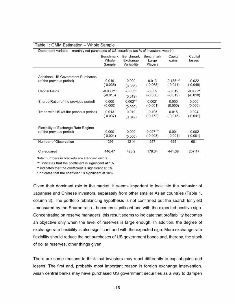
Table 1: GMM Estimation – Whole Sample Dependent variable – monthly net purchases of US securities (as % of investors’ wealth)
Benchmark Whole
Sample
Benchmark Exchange Variability
Benchmark Large
Players
Capital gains
Capital losses
Additional US Government Purchases (of the previous period) 0.019 0.009 0.013 -0.185*** -0.022 (-0.035) (0.036) (-0.068) (-0.041) (-0.048)
Capital Gains -0.038*** -0.033* -0.039 -0.019 -0.035** (-0.015) (0.019) (-0.030) (-0.019) (-0.018)
Sharpe Ratio (of the previous period) 0.000 0.002** 0.002* 0.000 0.000 (0.000) (0.000) (-0.001) (0.000) (0.000)
Trade with US (of the previous period) 0.013 0.019 -0.105 0.015 0.024 (-0.037) (0.042) (-0.172) (-0.048) (-0.041)
Flexibility of Exchange Rate Regime (of the previous period) 0.000 0.000 -0.027*** 0.001 -0.002 (-0.001) (0.000) (-0.008) (-0.001) (-0.001)
Number of Observation 1296 1214 257 695 601
Chi-squared 446.47 423.2 178.34 441.38 257.47
Note: numbers in brackets are standard errors. *** indicates that the coefficient is significant at 1%. ** indicates that the coefficient is significant at 5%. * indicates that the coefficient is significant at 10%.
Given their dominant role in the market, it seems important to look into the behavior of
Japanese and Chinese investors, separately from other smaller Asian countries (Table 1,
column 3). The portfolio rebalancing hypothesis is not confirmed but the search for yield
–measured by the Sharpe ratio - becomes significant and with the expected positive sign.
Concentrating on reserve managers, this result seems to indicate that profitability becomes
an objective only when the level of reserves is large enough. In addition, the degree of
exchange rate flexibility is also significant and with the expected sign: More exchange rate
flexibility should reduce the net purchases of US government bonds and, thereby, the stock
of dollar reserves, other things given.
There are some reasons to think that investors may react differently to capital gains and
losses. The first and, probably most important reason is foreign exchange intervention.
Asian central banks may have purchased US government securities as a way to dampen
- - 16
pressures for their currency to appreciate. This hypothesis, however, might be easier to test
later, when separating capital gains into exchange rate and yield related, as we shall do
later. Second, investors generally have to maintain a pre-determined level for each different
investment instrument – in line with their optimal portfolio - but this might be treated as a
minimum, so as to leave some space for active management on the upper side. Third, in the
specific case of official authorities, unrealized losses are generally reported to calculate net
profits but not unrealized gains. This might imply that unrealized losses trigger more action
(for the specific hypothesis of portfolio rebalancing namely buying additional US
government securities) because they have more direct consequences. In fact, we do find
evidence of such asymmetric behaviour and with the expected sign: portfolio rebalancing is
a significant determinant of net purchases of US securities only when there are capital
losses 27 (Table 1, column 5). Capital gains, in turn, do not appear to reduce purchases of
US securities (Table 1, column 4).
Given the large changes which have occurred in the period included in the above
exercise—such as the Asian crisis and the huge accumulation of reserves of the last few
years—we test for changes in reserve management and, particularly in our case, changes
in the determinants of net purchases of US treasuries by Asian investors. To this end, we
run rolling regressions of four years each. As Table 2 shows, portfolio rebalancing was a
significant determinant of net purchases of US treasury securities. This result also helps
explain the stability of the US dollar reserves in the years before the Asian crisis, at least as
US government securities are concerned. The opposite hypothesis – of “momentum
trading”- is never confirmed in the data.
Profitability considerations start becoming relevant, for the group of Asian countries as a
whole, in the last few years. This finding is very much in line with the responses given by
reserve managers in the Central Banking Publications survey. It also makes quite a lot of
sense that reserve managers are starting to worry about profitability when reserves are well
above what is needed to cover transaction needs28. Finally, transaction determinants are
significant only in a couple of instances but with the right sign. First, more trade with the US
27 The negative coefficient implies net purchases since capital losses are always negative, by definition. 28 Theoretical literature integrating the two—optimal reserve levels and currency decomposition of reserves (driven by the optimal portfolio theory)—hardly exists. We, thus, cannot assess the importance of the levels in the current analytical framework.
- - 17

contributes to larger net purchases of US government securities. Second, a more flexible
exchange rate regime, de facto, reduces such purchases.
- - 18
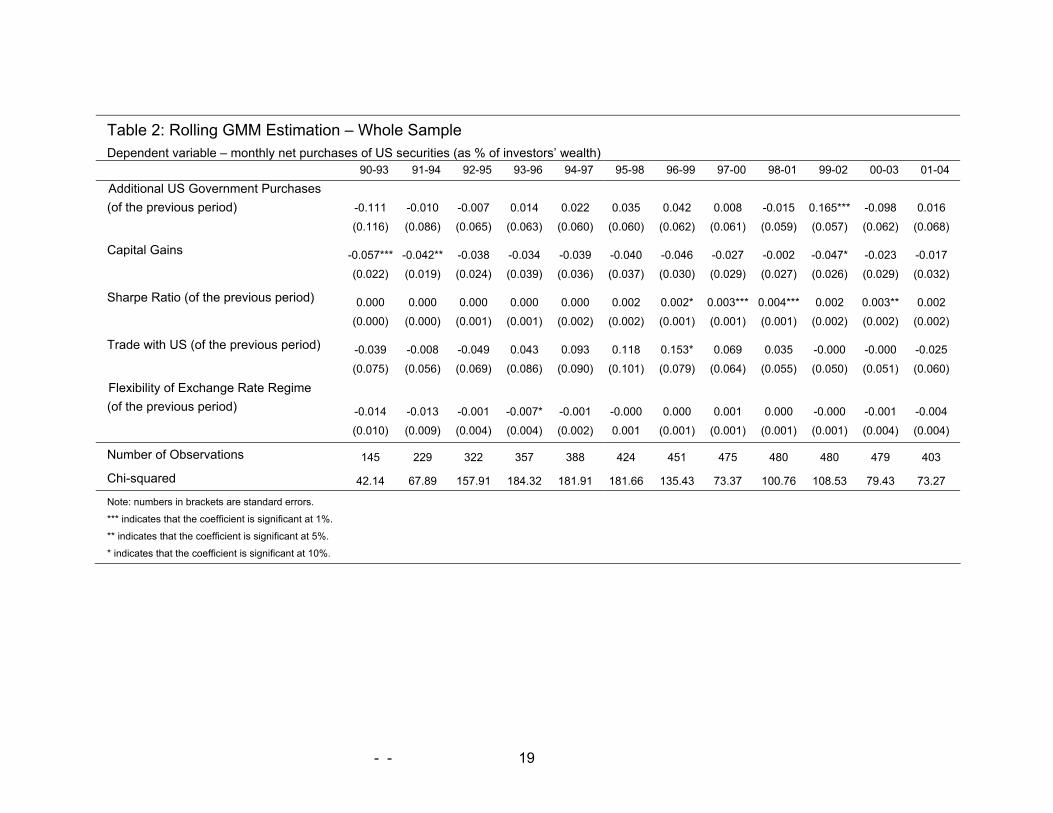
Table 2: Rolling GMM Estimation – Whole Sample Dependent variable – monthly net purchases of US securities (as % of investors’ wealth) 90-93 91-94 92-95 93-96 94-97 95-98 96-99 97-00 98-01 99-02 00-03 01-04
Additional US Government Purchases (of the previous period) -0.111 -0.010 -0.007 0.014 0.022 0.035 0.042 0.008 -0.015 0.165*** -0.098 0.016
(0.116)
(0.086) (0.065) (0.063) (0.060) (0.060) (0.062) (0.061) (0.059) (0.057) (0.062) (0.068)
Capital Gains -0.057*** -0.042** -0.038 -0.034 -0.039 -0.040 -0.046 -0.027 -0.002 -0.047* -0.023 -0.017
(0.022) (0.019) (0.024) (0.039) (0.036) (0.037) (0.030) (0.029) (0.027) (0.026) (0.029) (0.032)
Sharpe Ratio (of the previous period) 0.000 0.000 0.000 0.000 0.000 0.002 0.002* 0.003*** 0.004*** 0.002 0.003** 0.002
(0.000) (0.000) (0.001) (0.001) (0.002) (0.002) (0.001) (0.001) (0.001) (0.002) (0.002) (0.002)
Trade with US (of the previous period) -0.039 -0.008 -0.049 0.043 0.093 0.118 0.153* 0.069 0.035 -0.000 -0.000 -0.025
(0.075) (0.056) (0.069) (0.086) (0.090) (0.101) (0.079) (0.064) (0.055) (0.050) (0.051) (0.060)
Flexibility of Exchange Rate Regime (of the previous period) -0.014 -0.013 -0.001 -0.007* -0.001 -0.000 0.000 0.001 0.000 -0.000 -0.001 -0.004
(0.010) (0.009) (0.004) (0.004) (0.002) 0.001 (0.001) (0.001) (0.001) (0.001) (0.004) (0.004)
Number of Observations 145 229 322 357 388 424 451 475 480 480 479 403
Chi-squared 42.14 67.89 157.91 184.32 181.91 181.66 135.43 73.37 100.76 108.53 79.43 73.27
Note: numbers in brackets are standard errors.
*** indicates that the coefficient is significant at 1%.
** indicates that the coefficient is significant at 5%.
* indicates that the coefficient is significant at 10%.
- - 19
As before, we test for the existence of asymmetries for capital gains and losses using rolling
regressions. We find that the asymmetry is not as strong as that found for the full period:
investors seem to react to capital gains by reducing the net purchases of US government
securities during the last few years (Table A4 in the Appendix). Meanwhile, capital losses
induced the rebalancing in the early 90s (Table A5).
Another interesting question is whether investors react in the same way to exchange rate
related gains/losses as well as to interest rate related ones. Table 3 shows evidence that
Asian investors are more sensitive to interest rate changes in terms of rebalancing their
portfolios.29 One possible explanation for this result is that investors – and in particular
central banks - hedge some of the open exchange rate positions while they are fully
affected by interest rate changes.
Finally, we also test for asymmetries in interest rate and exchange rate movements. A
reduction in the return of US government securities (relative to euro-denominated ones),
which would imply a capital loss if realized, contributes to increasing the net purchases of
US government securities. This is in line with the result for capital losses as a whole and
consistent with the idea that return-related capital losses are those to which investors seem
to react the most. On the other hand, investors do not seem to react to losses stemming
from changes in the dollar-euro exchange rate.
In fact, as far as Asian currencies move closer to the dollar than the euro and Asian central
banks are known to intervene at times, we should have found that capital losses –because
of a dollar depreciation against the euro and, thereby, against the domestic currency – step
up purchases of US government bonds. The lack of significance of the coefficient for
exchange rate losses provides some indirect evidence – given the lack of data for a direct
test - against the concern that foreign exchange market intervention may be driving the net
purchases of US government securities.
29 Since there could be collinearity problems, we check the correlation between interest rate and exchange movements and find it to be low.
- - 20
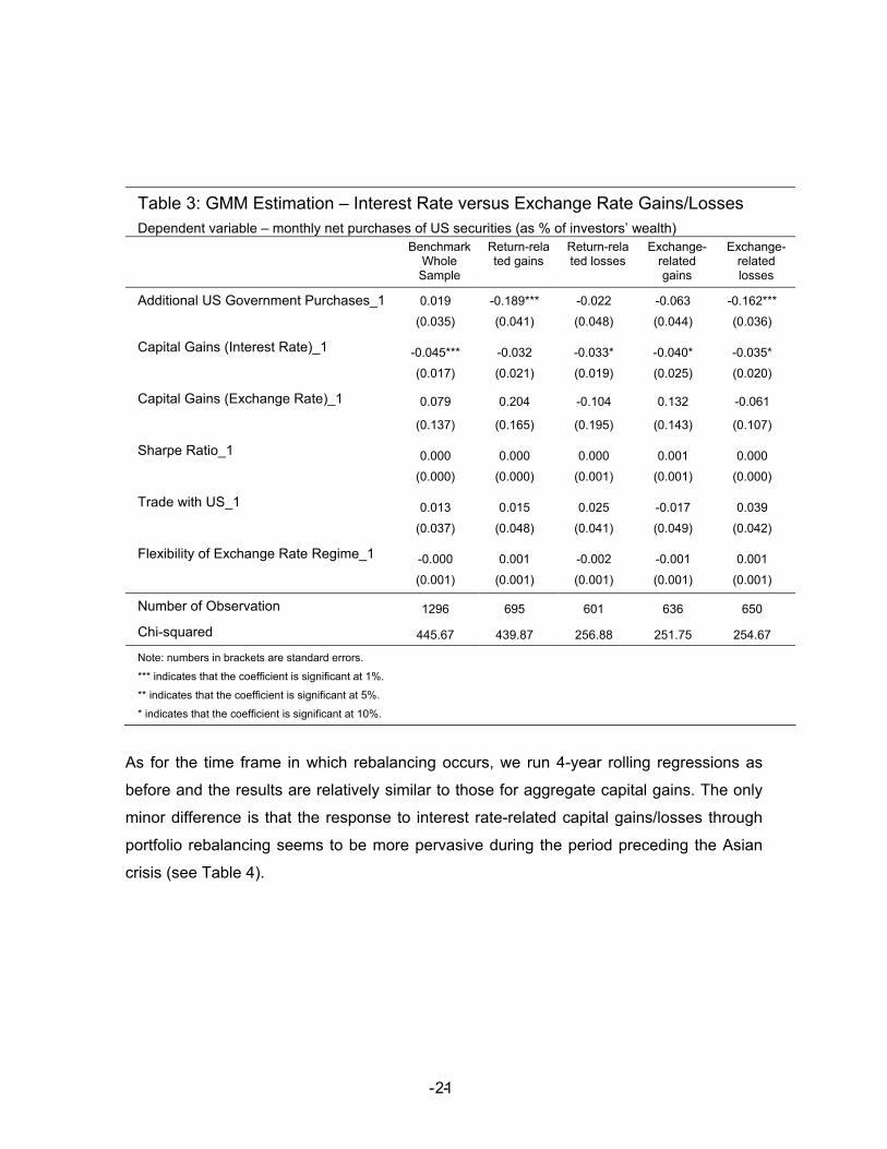
Table 3: GMM Estimation – Interest Rate versus Exchange Rate Gains/Losses Dependent variable – monthly net purchases of US securities (as % of investors’ wealth) Benchmark
Whole Sample
Return-related gains
Return-related losses
Exchange-related gains
Exchange-related losses
Additional US Government Purchases_1 0.019 -0.189*** -0.022 -0.063 -0.162***
(0.035) (0.041) (0.048) (0.044) (0.036)
Capital Gains (Interest Rate)_1 -0.045*** -0.032 -0.033* -0.040* -0.035*
(0.017) (0.021) (0.019) (0.025) (0.020)
Capital Gains (Exchange Rate)_1 0.079 0.204 -0.104 0.132 -0.061
(0.137) (0.165) (0.195) (0.143) (0.107)
Sharpe Ratio_1 0.000 0.000 0.000 0.001 0.000
(0.000) (0.000) (0.001) (0.001) (0.000)
Trade with US_1 0.013 0.015 0.025 -0.017 0.039
(0.037) (0.048) (0.041) (0.049) (0.042)
Flexibility of Exchange Rate Regime_1 -0.000 0.001 -0.002 -0.001 0.001
(0.001) (0.001) (0.001) (0.001) (0.001)
Number of Observation 1296 695 601 636 650
Chi-squared 445.67 439.87 256.88 251.75 254.67
Note: numbers in brackets are standard errors.
*** indicates that the coefficient is significant at 1%.
** indicates that the coefficient is significant at 5%.
* indicates that the coefficient is significant at 10%.
As for the time frame in which rebalancing occurs, we run 4-year rolling regressions as
before and the results are relatively similar to those for aggregate capital gains. The only
minor difference is that the response to interest rate-related capital gains/losses through
portfolio rebalancing seems to be more pervasive during the period preceding the Asian
crisis (see Table 4).
- - 21
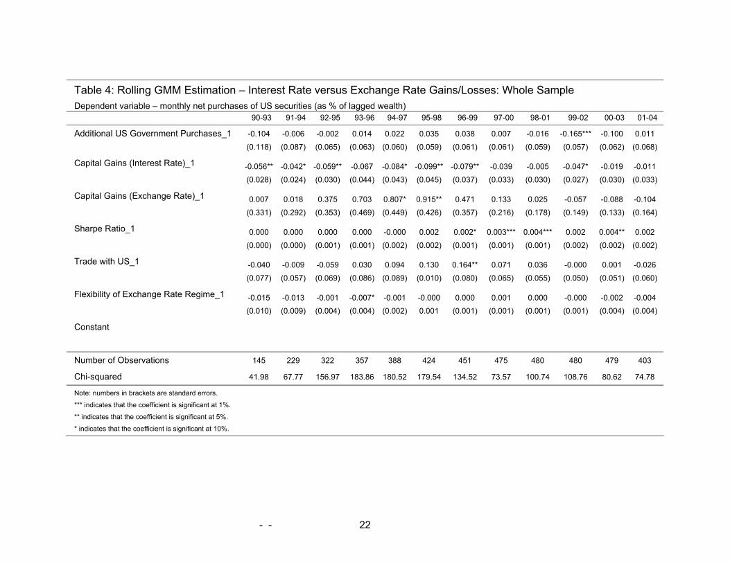
Table 4: Rolling GMM Estimation – Interest Rate versus Exchange Rate Gains/Losses: Whole Sample Dependent variable – monthly net purchases of US securities (as % of lagged wealth) 90-93 91-94 92-95 93-96 94-97 95-98 96-99 97-00 98-01 99-02 00-03 01-04
Additional US Government Purchases_1 -0.104 -0.006 -0.002 0.014 0.022 0.035 0.038 0.007 -0.016 -0.165*** -0.100 0.011
(0.118)
(0.087) (0.065) (0.063) (0.060) (0.059) (0.061) (0.061) (0.059) (0.057) (0.062) (0.068)
Capital Gains (Interest Rate)_1 -0.056** -0.042* -0.059** -0.067 -0.084* -0.099** -0.079** -0.039 -0.005 -0.047* -0.019 -0.011
(0.028) (0.024) (0.030) (0.044) (0.043) (0.045) (0.037) (0.033) (0.030) (0.027) (0.030) (0.033)
Capital Gains (Exchange Rate)_1 0.007 0.018 0.375 0.703 0.807* 0.915** 0.471 0.133 0.025 -0.057 -0.088 -0.104
(0.331) (0.292) (0.353) (0.469) (0.449) (0.426) (0.357) (0.216) (0.178) (0.149) (0.133) (0.164)
Sharpe Ratio_1 0.000 0.000 0.000 0.000 -0.000 0.002 0.002* 0.003*** 0.004*** 0.002 0.004** 0.002
(0.000) (0.000) (0.001) (0.001) (0.002) (0.002) (0.001) (0.001) (0.001) (0.002) (0.002) (0.002)
Trade with US_1 -0.040 -0.009 -0.059 0.030 0.094 0.130 0.164** 0.071 0.036 -0.000 0.001 -0.026
(0.077) (0.057) (0.069) (0.086) (0.089) (0.010) (0.080) (0.065) (0.055) (0.050) (0.051) (0.060)
Flexibility of Exchange Rate Regime_1 -0.015 -0.013 -0.001 -0.007* -0.001 -0.000 0.000 0.001 0.000 -0.000 -0.002 -0.004
(0.010) (0.009) (0.004) (0.004) (0.002) 0.001 (0.001) (0.001) (0.001) (0.001) (0.004) (0.004)
Constant
Number of Observations 145 229 322 357 388 424 451 475 480 480 479 403
Chi-squared 41.98 67.77 156.97 183.86 180.52 179.54 134.52 73.57 100.74 108.76 80.62 74.78
Note: numbers in brackets are standard errors.
*** indicates that the coefficient is significant at 1%.
** indicates that the coefficient is significant at 5%.
* indicates that the coefficient is significant at 10%.
- - 22
Finally, we explore whether all Asian countries in our sample behave similarly. To this end,
we run 2SLS regression by country so as to take care of potential endogeneity. We use the
lagged dependent variable as an instrument. We find confirmation of portfolio rebalancing
for Indonesian, Malaysian, and Chinese investors. On the contrary, momentum trading is
confirmed for Philippine investors. For Japan and Philippines, the search for yield is found
significant and with the expected sign: the higher the expected risk-adjusted yield, the more
net purchases of US government securities there will be. Finally, in Korea and Indonesia, an
increase in the share of trade with the US steps up the next purchases of US government
securities. Interestingly, the opposite sign is found significant for Japan. Finally, a more
flexible exchange rate regime does reduce China’s purchases of US government securities.
- - 23
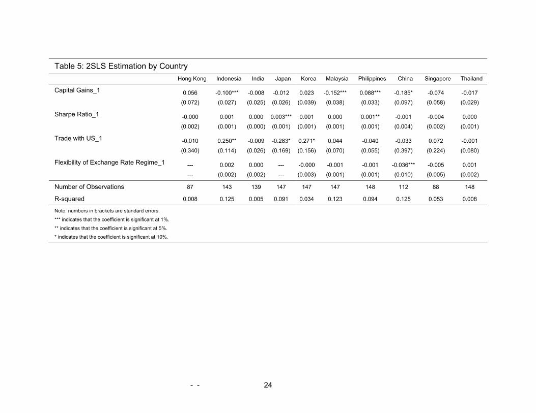
Table 5: 2SLS Estimation by Country Hong Kong Indonesia India Japan Korea Malaysia Philippines China Singapore Thailand
Capital Gains_1 0.056 -0.100*** -0.008 -0.012 0.023 -0.152*** 0.088*** -0.185* -0.074 -0.017
(0.072)
(0.027) (0.025) (0.026) (0.039) (0.038) (0.033) (0.097) (0.058) (0.029)
Sharpe Ratio_1 -0.000 0.001 0.000 0.003*** 0.001 0.000 0.001** -0.001 -0.004 0.000
(0.002) (0.001) (0.000) (0.001) (0.001) (0.001) (0.001) (0.004) (0.002) (0.001)
Trade with US_1 -0.010 0.250** -0.009 -0.283* 0.271* 0.044 -0.040 -0.033 0.072 -0.001
(0.340) (0.114) (0.026) (0.169) (0.156) (0.070) (0.055) (0.397) (0.224) (0.080)
Flexibility of Exchange Rate Regime_1 --- 0.002 0.000 --- -0.000 -0.001 -0.001 -0.036*** -0.005 0.001
--- (0.002) (0.002) --- (0.003) (0.001) (0.001) (0.010) (0.005) (0.002)
Number of Observations 87 143 139 147 147 147 148 112 88 148
R-squared 0.008 0.125 0.005 0.091 0.034 0.123 0.094 0.125 0.053 0.008
Note: numbers in brackets are standard errors.
*** indicates that the coefficient is significant at 1%.
** indicates that the coefficient is significant at 5%.
* indicates that the coefficient is significant at 10%.
- - 24
5. Conclusions
This paper explores whether Asian investors – and in particular official authorities -
rebalance their portfolios as a consequence of capital gains or losses. Portfolio rebalancing
would imply that investors increase their net purchases of US government securities after
incurring capital losses so as to maintain their desired portfolio. Instead, they should sell
securities after obtaining capital gains to achieve the same objective.
We choose the market of US government debt securities since we need to concentrate on
one single investment instrument (in one single currency) to readily calculate capital gains
and losses. In addition, this is the most widely used instrument by central banks to hold their
reserves in dollar. Finally, we focus on Asian countries because they are very important
investors in the market of US government securities and because their activity is
concentrated in the hands of central banks. Their purchases of US government securities
can shed some light of their reserve management strategies.
We find evidence of portfolio rebalancing for a group of 10 Asian countries for the period
from 1990 until end 2004 although it was more significant in the years before the Asian
crisis. In the last few years, profitability considerations are more and more relevant for Asian
investors. In addition, capital losses tend to contribute more to additional net purchases of
US securities than capital gains do to reducing such purchases. This could be due to the
way investment strategies are designed but also to the fact that official investors generally
treat unrealized losses as actual losses but not unrealized gains. Finally, we find that Asian
investors are more sensitive to interest rate movements than to exchange rate movements
when rebalancing their portfolio. This probably reflects more hedging of foreign exchange
risk than of interest rate risk.
The evidence found in favor of portfolio rebalancing by Asian investors points to their
stabilizing role in that market. In fact, portfolio rebalancing reduces the likelihood of
one-directional movements in their purchases of US Treasury securities, which- given their
size in the market and the size of the US fiscal deficit– may have positive systemic
implications, in terms of reduction of global financial market volatility. This statement is
especially true for the years prior to the Asian crisis. In most recent years, the chase for
return has become more relevant in explaining net purchases of US treasury securities.
- - 25

This might have brought some more volatility to the share of US dollar reserves, other
factors given.
- - 26
REFERENCES
Arellano, M. and S. Bond. 1991. Some tests of specification for panel data: Monte Carlo evidence and an application to employment equations. The Review of Economic Studies 58: 277-297.
Bank of Japan, 2005. “Basic Guidelines for the Management of External Assets Held by Bank of Japan”, available at http://www.boj.or.jp/en/type/law/hyoryo01.htm.
Ben-Bassat, Avraham, 1980. “The Optimal Composition of Foreign Exchange Reserves,” Journal of International Economics: 10; 285-295.
Bohn, Henning and Linda Tesar, 1996. “US Equity Investment in Foreign Markets: Portfolio Rebalancing or Return Chasing?”, American Economic Review, Vol. 86, No 2, Paper and Proceedings of the Hundredth and Eighth Annual Meeting of the American Economic Association.
Carver, Nick, and Robert Pringle, 2004. “Survey of Central Bank Risk Managers” in New Horizons in Central Bank Risk Management”, R. Pringle and N. Carver eds. Central Banking Publications Ltd
Claessens, Stijn, and Jerome Kreuser, 2004. “A framework for strategic foreign reserves risk management”, in Risk Management for Central Bank Foreign Reserves. Bernadell et al. eds. European Central Bank. Dooley, Michael, Saul Lizondo and Donald Mathieson, 1989. “The Currency Composition of Foreign Exchange Reserves”, IMF Staff Papers, Vol.36 No 2. Fisher, Stephen J. and Min C. Lie, 2004. “Asset allocation for central banks: optimally combining liquidity, duration, currency and non-government risk” in Risk Management for Central Bank Foreign Reserves. Bernadell et al. eds. European Central Bank. Hau, Harald and Helene Rey, 2004. “Can Portfolio Rebalancing Explain the Dynamics of Equity Returns, Equity Flows and Exchange Rates?”, mimeo McCauley, Robert and Ben Fung, 2003. “Choosing Instruments in Managing Foreign Exchange Reserves”, BIS Quarterly Bulletin, March 2003. Reinhart, Carmen M. and Kenneth S. Rogoff, 2004. “The Modern History of Exchange Rate Arrangements: A Reinterpretation,” Quarterly Journal of Economics, vol. CXIX Issue 1: 1-48.
Truman Edwin and Anne Wong, 2006. “The Case for an International Diversification
Standard”.
Wooldrigde, Philip, 2006. “The Changing Composition of Official Reserves”, BIS Quarterly
Bulletin, September 2006.
- - 27
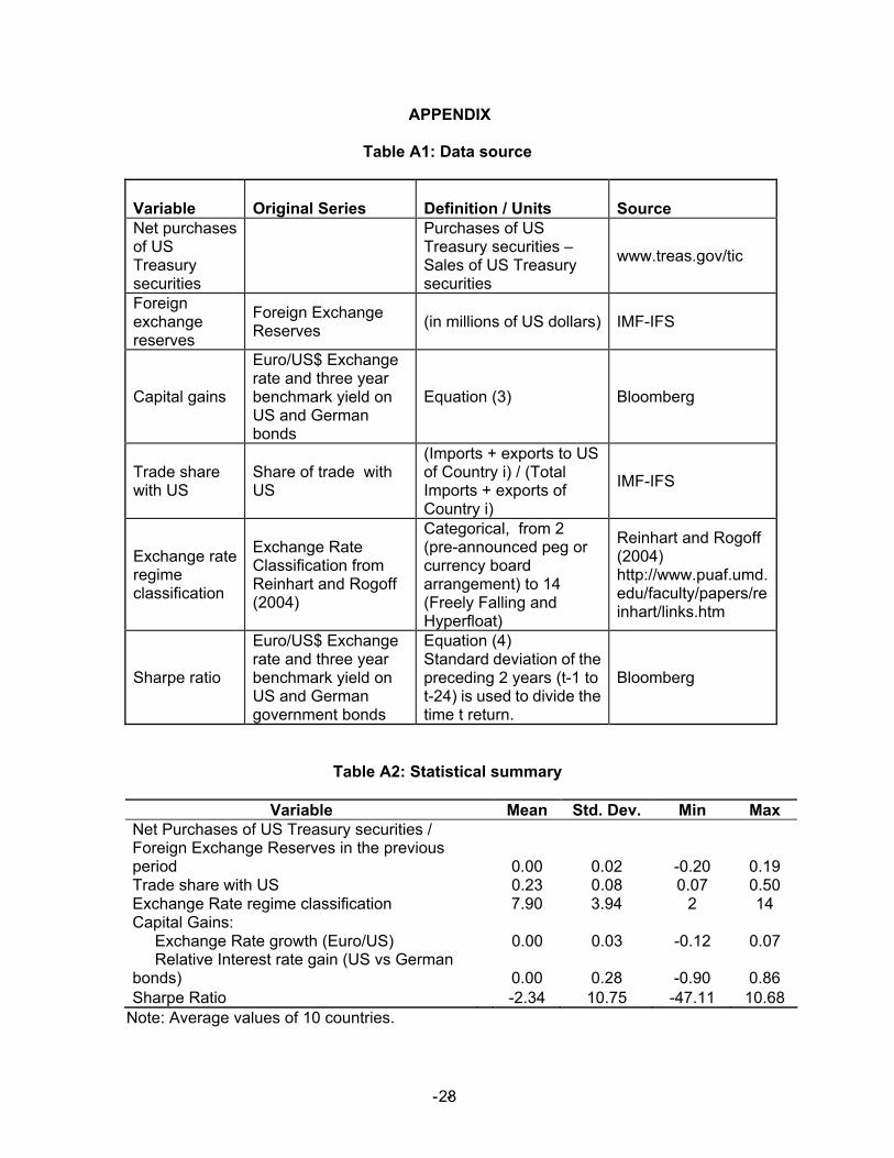
APPENDIX
Table A1: Data source
Variable Original Series Definition / Units Source
Net purchases of US Treasury securities
Purchases of US Treasury securities – Sales of US Treasury securities
www.treas.gov/tic
Foreign exchange reserves
Foreign Exchange Reserves (in millions of US dollars) IMF-IFS
Capital gains
Euro/US$ Exchange rate and three year benchmark yield on US and German bonds
Equation (3) Bloomberg
Trade share with US
Share of trade with US
(Imports + exports to US of Country i) / (Total Imports + exports of Country i)
IMF-IFS
Exchange rate regime classification
Exchange Rate Classification from Reinhart and Rogoff (2004)
Categorical, from 2 (pre-announced peg or currency board arrangement) to 14 (Freely Falling and Hyperfloat)
Reinhart and Rogoff (2004) http://www.puaf.umd.edu/faculty/papers/reinhart/links.htm
Sharpe ratio
Euro/US$ Exchange rate and three year benchmark yield on US and German government bonds
Equation (4) Standard deviation of the preceding 2 years (t-1 to t-24) is used to divide the time t return.
Bloomberg
Table A2: Statistical summary
Variable Mean Std. Dev. Min Max Net Purchases of US Treasury securities / Foreign Exchange Reserves in the previous period 0.00 0.02 -0.20 0.19 Trade share with US 0.23 0.08 0.07 0.50 Exchange Rate regime classification 7.90 3.94 2 14 Capital Gains: Exchange Rate growth (Euro/US) 0.00 0.03 -0.12 0.07 Relative Interest rate gain (US vs German bonds) 0.00 0.28 -0.90 0.86 Sharpe Ratio -2.34 10.75 -47.11 10.68
Note: Average values of 10 countries.
- - 28
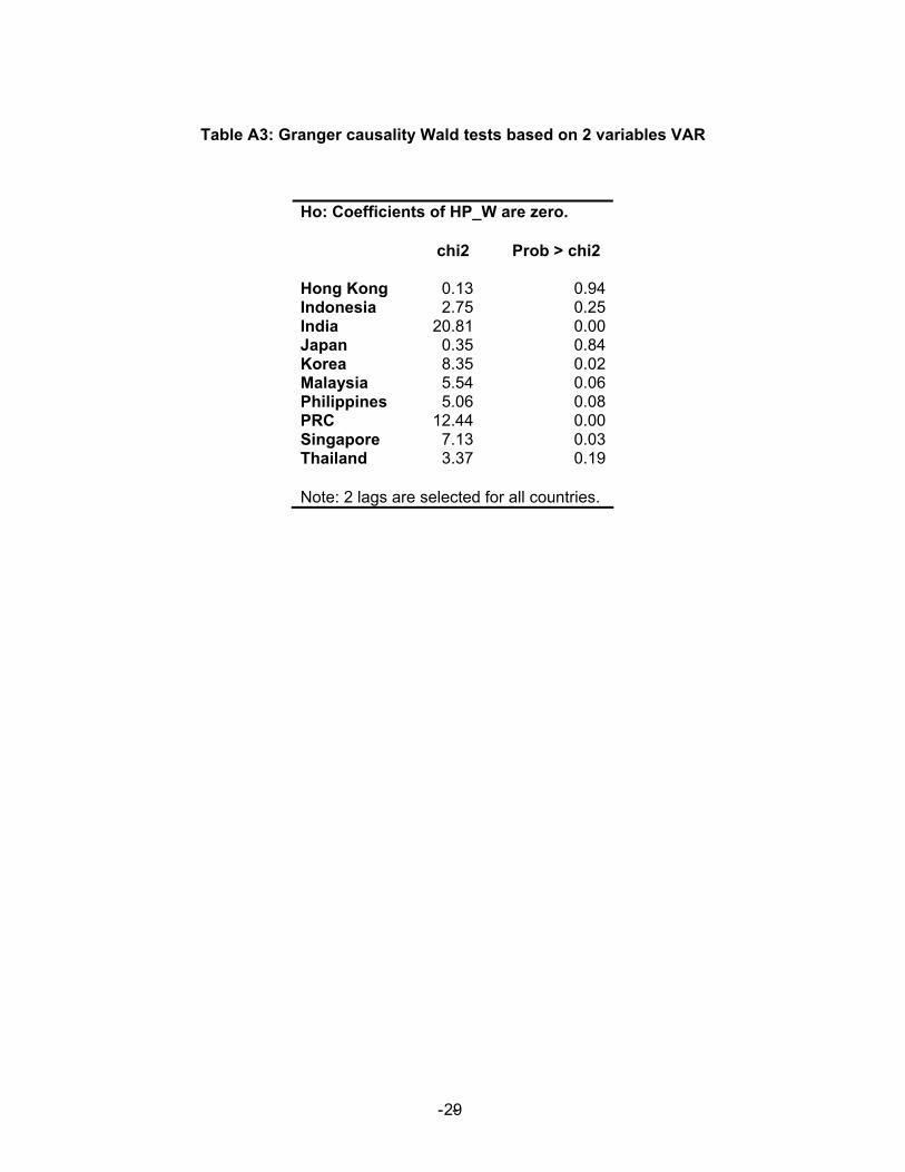
Table A3: Granger causality Wald tests based on 2 variables VAR
Ho: Coefficients of HP_W are zero.
chi2 Prob > chi2 Hong Kong 0.13 0.94 Indonesia 2.75 0.25 India 20.81 0.00 Japan 0.35 0.84 Korea 8.35 0.02 Malaysia 5.54 0.06 Philippines 5.06 0.08 PRC 12.44 0.00 Singapore 7.13 0.03 Thailand 3.37 0.19 Note: 2 lags are selected for all countries.
- - 29
Table A4: Rolling GMM Estimation – Sample of Positive Gains Dependent variable – monthly net purchases of US securities (as % of lagged investors’ wealth) 90-93 91-94 92-95 93-96 94-97 95-98 96-99 97-00 98-01 99-02 00-03 01-04
Additional US Government Purchases
(of the previous period)
-0.613*** -0.528*** -0.260*** -0.191*** -0.095 -0.080 -0.066 -0.124 -0.162** -0.214*** -0.218*** -0.249***
(0.139) (0.079) (0.073) (0.075) (0.078) (0.076) (0.092) (0.077) (0.070) (0.064 (0.070) (0.087) Capital Gains -0.015 -0.008 0.021 0.051 -0.051 -0.049 -0.063 -0.071** -0.012 -0.074** -0.035 -0.042
(0.029) (0.022) (0.032) (0.048) (0.047) (0.052) (0.039) (0.036) (0.035) (0.031 (0.030) (0.036) Sharpe Ratio (of the
previous period) 0.000 0.000 -0.000 0.000 -0.000 0.002 0.003** 0.003*** 0.003*** 0.002 0.003 0.003
(0.000) (0.000) (0.000) (0.002) (0.003) (0.002) (0.001) (0.001) (0.001) (0.002) (0.002) (0.002) Trade with US (of the
previous period) -0.034 -0.000 -0.025 0.013 0.076 0.045 0.106 0.021 0.016 0.031 0.014 -0.012
(0.100) (0.075) (0.108) (0.120) (0.127) (0.128) (0.109) (0.082) (0.062) (0.058) (0.054) (0.061) Flexibility of Exchange
Rate Regime (of the previous period)
-0.020* -0.021** -0.017 -0.015** 0.000 0.001 0.000 0.002** 0.002* 0.000 -0.001 -0.003
(0.009) (0.009) (0.014) (0.006) (0.002) (0.002) (0.001) (0.001) (0.001) (0.001) (0.003) (0.003) Number of
Observations 61 91 139 156 205 235 228 270 291 311 320 238
Chi-squared 58.76 80.04 170.1 162.6 146.9 152.7 61.51 41.21 77.47 75.43 54.51 49.22
Note: numbers in brackets are standard errors.
*** indicates that the coefficient is significant at 1%.
** indicates that the coefficient is significant at 5%.
* indicates that the coefficient is significant at 10%.
- - 30
Table A5: Rolling GMM Estimation – Sample of Negative Gains Dependent variable – monthly net purchases of US securities (as % of lagged investors’ wealth) 90-93 91-94 92-95 93-96 94-97 95-98 96-99 97-00 98-01 99-02 00-03 01-04
Additional US Government Purchases
(of the previous period) -0.367*** -0.206** -0.170** -0.134* 0.003 0.004 0.010 0.005 0.041 -0.103 -0.016 0.114
(0.093) (0.087) (0.085) (0.081) (0.087) (0.083) (0.074) (0.087) (0.096) (0.098) (0.108) (0.099) Capital Gains -0.112*** -0.051** -0.046** -0.022 -0.016 -0.091 -0.056 -0.017 0.001 0.026 0.054 0.040
(0.027) (0.022) (0.023) (0.032) (0.030) (0.037) (0.035) (0.051) (0.050) (0.044) (0.048) (0.045) Sharpe Ratio (of the previous
period) -0.000 0.000 0.000 -0.000 -0.002 -0.005* -0.003 -0.001 0.001 0.003 0.003 0.001
(0.000) (0.000) (0.000) (0.001) (0.002) (0.003) (0.002) (0.002) (0.002) (0.002) (0.002) (0.002) Trade with US (of the previous
period) 0.035 0.020 0.002 0.106 0.125 0.219** 0.136 0.061 0.021 -0.069 -0.078 -0.130
(0.071) (0.055) (0.056) (0.078) (0.090) (0.106) (0.088) (0.075) (0.081) (0.078) (0.089) (0.095) Flexibility of Exchange Rate
Regime (of the previous period)
-0.051*** -0.030* -0.001 0.000 -0.000 -0.000 -0.001 -0.001 -0.001 -0.004 0.008 ---
(0.019) (0.014) (0.003) (0.006) (0.003) (0.001) (0.001) (0.001) (0.001) (0.009) (0.011)
Number of Observations 84 138 183 201 183 189 223 205 189 169 159 165
Chi-squared 43.2 67.06 121.1 133.6 120.1 104.3 90.88 46.18 40.74 45.11 24.79 26.51
Note: numbers in brackets are standard errors.
*** indicates that the coefficient is significant at 1%.
** indicates that the coefficient is significant at 5%.
* indicates that the coefficient is significant at 10%.
Flexibility of Exchange Rate Regime is dropped for the period between 01 and 04 due to collinearity.
- - 31