DNA Fragment Analysis by Capillary Electrophoresis
220
USER GUIDE For Research Use Only. Not intended for use in diagnostic procedures. DNA Fragment Analysis by Capillary Electrophoresis Publication Number 4474504 Revision B
Transcript of DNA Fragment Analysis by Capillary Electrophoresis

USER GUIDE
For Research Use Only. Not intended for use in diagnostic procedures.
DNA Fragment Analysis by Capillary Electrophoresis
Publication Number 4474504Revision B

For Research Use Only. Not intended for use in diagnostic procedures.The information in this guide is subject to change without notice.
DISCLAIMER
LIFE TECHNOLOGIES CORPORATION AND/OR ITS AFFILIATE(S) DISCLAIM ALL WARRANTIES WITH RESPECT TO THIS DOCUMENT, EXPRESSED OR IMPLIED, INCLUDING BUT NOT LIMITED TO THOSE OF MERCHANTABILITY, FITNESS FOR A PARTICULAR PURPOSE, OR NON-INFRINGEMENT. TO THE EXTENT ALLOWED BY LAW, IN NO EVENT SHALL LIFE TECHNOLOGIES AND/OR ITS AFFILIATE(S) BE LIABLE, WHETHER IN CONTRACT, TORT, WARRANTY, OR UNDER ANY STATUTE OR ON ANY OTHER BASIS FOR SPECIAL, INCIDENTAL, INDIRECT, PUNITIVE, MULTIPLE OR CONSEQUENTIAL DAMAGES IN CONNECTION WITH OR ARISING FROM THIS DOCUMENT, INCLUDING BUT NOT LIMITED TO THE USE THEREOF.
TRADEMARKS
All trademarks are the property of Thermo Fisher Scientific and its subsidiaries unless otherwise specified.
AmpErase, AmpliTaq, AmpliTaq Gold, and TaqMan are registered trademarks of Roche Molecular Systems, Inc.
AFLP is a registered trademark of Keygene N.V.
Millipore is a registered trademark of Merck KGaA.
© 2014 Thermo Fisher Scientific Inc. All rights reserved.

Contents
3DNA Fragment Analysis by Capillary Electrophoresis
About This Guide . . . . . . . . . . . . . . . . . . . . . . . . . . . . . . . . . . . . . . . . . . . . . . . . 13
Revision history . . . . . . . . . . . . . . . . . . . . . . . . . . . . . . . . . . . . . . . . . . . . . . . . . . . . . . . . . . . . . . . . . . . . . . 13
Purpose . . . . . . . . . . . . . . . . . . . . . . . . . . . . . . . . . . . . . . . . . . . . . . . . . . . . . . . . . . . . . . . . . . . . . . . . . . . . 13
Prerequisites . . . . . . . . . . . . . . . . . . . . . . . . . . . . . . . . . . . . . . . . . . . . . . . . . . . . . . . . . . . . . . . . . . . . . . . . 13
Structure of this guide . . . . . . . . . . . . . . . . . . . . . . . . . . . . . . . . . . . . . . . . . . . . . . . . . . . . . . . . . . . . . . . . 14
■ CHAPTER 1 Introduction to Fragment Analysis . . . . . . . . . . . . . . . . . . 15
Fragment analysis versus sequencing…what is the difference? . . . . . . . . . . . . . . . . . . . . . . . . . . . . 15Fragment analysis . . . . . . . . . . . . . . . . . . . . . . . . . . . . . . . . . . . . . . . . . . . . . . . . . . . . . . . . . . . . . . . 15Sequencing . . . . . . . . . . . . . . . . . . . . . . . . . . . . . . . . . . . . . . . . . . . . . . . . . . . . . . . . . . . . . . . . . . . . . 16
What can I do with fragment analysis? . . . . . . . . . . . . . . . . . . . . . . . . . . . . . . . . . . . . . . . . . . . . . . . . . . 16Types of applications . . . . . . . . . . . . . . . . . . . . . . . . . . . . . . . . . . . . . . . . . . . . . . . . . . . . . . . . . . . . . 16Applications described in this guide . . . . . . . . . . . . . . . . . . . . . . . . . . . . . . . . . . . . . . . . . . . . . . . . 17
What is capillary electrophoresis? . . . . . . . . . . . . . . . . . . . . . . . . . . . . . . . . . . . . . . . . . . . . . . . . . . . . . . 18
Fragment analysis workflow . . . . . . . . . . . . . . . . . . . . . . . . . . . . . . . . . . . . . . . . . . . . . . . . . . . . . . . . . . 19
■ CHAPTER 2 Experimental Design . . . . . . . . . . . . . . . . . . . . . . . . . . . . . . . 21
Experimental design considerations . . . . . . . . . . . . . . . . . . . . . . . . . . . . . . . . . . . . . . . . . . . . . . . . . . . . 21
DNA polymerase enzymes . . . . . . . . . . . . . . . . . . . . . . . . . . . . . . . . . . . . . . . . . . . . . . . . . . . . . . . . . . . . 22Overview . . . . . . . . . . . . . . . . . . . . . . . . . . . . . . . . . . . . . . . . . . . . . . . . . . . . . . . . . . . . . . . . . . . . . . . 22Derivatives of Tth DNA polymerase . . . . . . . . . . . . . . . . . . . . . . . . . . . . . . . . . . . . . . . . . . . . . . . . 24Enzyme characteristics . . . . . . . . . . . . . . . . . . . . . . . . . . . . . . . . . . . . . . . . . . . . . . . . . . . . . . . . . . 24
Fluorescent labeling methods . . . . . . . . . . . . . . . . . . . . . . . . . . . . . . . . . . . . . . . . . . . . . . . . . . . . . . . . . 25
Singleplexing versus multiplexing . . . . . . . . . . . . . . . . . . . . . . . . . . . . . . . . . . . . . . . . . . . . . . . . . . . . . . 26Singleplexing . . . . . . . . . . . . . . . . . . . . . . . . . . . . . . . . . . . . . . . . . . . . . . . . . . . . . . . . . . . . . . . . . . . 26Multiplexing . . . . . . . . . . . . . . . . . . . . . . . . . . . . . . . . . . . . . . . . . . . . . . . . . . . . . . . . . . . . . . . . . . . . 26Multiplexing (pooling) strategies . . . . . . . . . . . . . . . . . . . . . . . . . . . . . . . . . . . . . . . . . . . . . . . . . . . 27Multiplex design software . . . . . . . . . . . . . . . . . . . . . . . . . . . . . . . . . . . . . . . . . . . . . . . . . . . . . . . . 28Multiplexing guidelines . . . . . . . . . . . . . . . . . . . . . . . . . . . . . . . . . . . . . . . . . . . . . . . . . . . . . . . . . . 28
Primer design guidelines . . . . . . . . . . . . . . . . . . . . . . . . . . . . . . . . . . . . . . . . . . . . . . . . . . . . . . . . . . . . . 29Primer design criteria . . . . . . . . . . . . . . . . . . . . . . . . . . . . . . . . . . . . . . . . . . . . . . . . . . . . . . . . . . . 29Primer design software . . . . . . . . . . . . . . . . . . . . . . . . . . . . . . . . . . . . . . . . . . . . . . . . . . . . . . . . . . 29Factors affecting Tm and primer annealing . . . . . . . . . . . . . . . . . . . . . . . . . . . . . . . . . . . . . . . . . 30Effects of template secondary structure . . . . . . . . . . . . . . . . . . . . . . . . . . . . . . . . . . . . . . . . . . . . 31Selective amplification . . . . . . . . . . . . . . . . . . . . . . . . . . . . . . . . . . . . . . . . . . . . . . . . . . . . . . . . . . . 31Preferential amplification . . . . . . . . . . . . . . . . . . . . . . . . . . . . . . . . . . . . . . . . . . . . . . . . . . . . . . . . 31

4 DNA Fragment Analysis by Capillary Electrophoresis
Contents
Non-specific amplification . . . . . . . . . . . . . . . . . . . . . . . . . . . . . . . . . . . . . . . . . . . . . . . . . . . . . . . . 32Minimizing binding to other primers . . . . . . . . . . . . . . . . . . . . . . . . . . . . . . . . . . . . . . . . . . . . . . . . 32Post-amplification manipulations . . . . . . . . . . . . . . . . . . . . . . . . . . . . . . . . . . . . . . . . . . . . . . . . . . 33Addition of 3' A nucleotide by Taq polymerase . . . . . . . . . . . . . . . . . . . . . . . . . . . . . . . . . . . . . . . . 33
Dyes . . . . . . . . . . . . . . . . . . . . . . . . . . . . . . . . . . . . . . . . . . . . . . . . . . . . . . . . . . . . . . . . . . . . . . . . . . . . . . . . 36Dyes and chemical forms . . . . . . . . . . . . . . . . . . . . . . . . . . . . . . . . . . . . . . . . . . . . . . . . . . . . . . . . . 36Multicomponent analysis with fluorescent dyes . . . . . . . . . . . . . . . . . . . . . . . . . . . . . . . . . . . . . . 36Factors that affect dye signal . . . . . . . . . . . . . . . . . . . . . . . . . . . . . . . . . . . . . . . . . . . . . . . . . . . . . . 37Emission and absorption (excitation) wavelengths and relative intensities . . . . . . . . . . . . . . . 38Points to consider when selecting dyes for custom primers . . . . . . . . . . . . . . . . . . . . . . . . . . . 39Example: selecting dyes . . . . . . . . . . . . . . . . . . . . . . . . . . . . . . . . . . . . . . . . . . . . . . . . . . . . . . . . . . 39
Dye sets . . . . . . . . . . . . . . . . . . . . . . . . . . . . . . . . . . . . . . . . . . . . . . . . . . . . . . . . . . . . . . . . . . . . . . . . . . . . . 41Dye sets and matrix standards . . . . . . . . . . . . . . . . . . . . . . . . . . . . . . . . . . . . . . . . . . . . . . . . . . . . . 41Creating a custom dye set . . . . . . . . . . . . . . . . . . . . . . . . . . . . . . . . . . . . . . . . . . . . . . . . . . . . . . . . . 41
Size standards . . . . . . . . . . . . . . . . . . . . . . . . . . . . . . . . . . . . . . . . . . . . . . . . . . . . . . . . . . . . . . . . . . . . . . . 42Functions of a size standard . . . . . . . . . . . . . . . . . . . . . . . . . . . . . . . . . . . . . . . . . . . . . . . . . . . . . . . 42Size-standard peak intensity . . . . . . . . . . . . . . . . . . . . . . . . . . . . . . . . . . . . . . . . . . . . . . . . . . . . . . 42Selecting a GeneScan™ size standard . . . . . . . . . . . . . . . . . . . . . . . . . . . . . . . . . . . . . . . . . . . . . . . 43Peaks not used for sizing . . . . . . . . . . . . . . . . . . . . . . . . . . . . . . . . . . . . . . . . . . . . . . . . . . . . . . . . . 43Preparing a size standard . . . . . . . . . . . . . . . . . . . . . . . . . . . . . . . . . . . . . . . . . . . . . . . . . . . . . . . . . 43GeneScan™ 120 LIZ® Size Standard . . . . . . . . . . . . . . . . . . . . . . . . . . . . . . . . . . . . . . . . . . . . . . . . . 44GeneScan™ 500 LIZ® Size Standard . . . . . . . . . . . . . . . . . . . . . . . . . . . . . . . . . . . . . . . . . . . . . . . . . 44GeneScan™ 600 LIZ® and GeneScan™ 600 LIZ® v2.0 Size Standards . . . . . . . . . . . . . . . . . . . . 45GeneScan™ 1200 LIZ® Size Standard . . . . . . . . . . . . . . . . . . . . . . . . . . . . . . . . . . . . . . . . . . . . . . . 47GeneScan™ 350 ROX™ Size Standard . . . . . . . . . . . . . . . . . . . . . . . . . . . . . . . . . . . . . . . . . . . . . . . . 49GeneScan™ 400HD ROX™ Size Standard . . . . . . . . . . . . . . . . . . . . . . . . . . . . . . . . . . . . . . . . . . . . . 49GeneScan™ 500 ROX™ Size Standard . . . . . . . . . . . . . . . . . . . . . . . . . . . . . . . . . . . . . . . . . . . . . . . . 50GeneScan™ 1000 ROX™ Size Standard . . . . . . . . . . . . . . . . . . . . . . . . . . . . . . . . . . . . . . . . . . . . . . . 51
Ordering custom primers . . . . . . . . . . . . . . . . . . . . . . . . . . . . . . . . . . . . . . . . . . . . . . . . . . . . . . . . . . . . . . 52
Testing the primers and optimizing conditions with test DNA panel . . . . . . . . . . . . . . . . . . . . . . . . . . 52Testing . . . . . . . . . . . . . . . . . . . . . . . . . . . . . . . . . . . . . . . . . . . . . . . . . . . . . . . . . . . . . . . . . . . . . . . . . 52Optimizing conditions . . . . . . . . . . . . . . . . . . . . . . . . . . . . . . . . . . . . . . . . . . . . . . . . . . . . . . . . . . . . 53
■ CHAPTER 3 Optimizing PCR . . . . . . . . . . . . . . . . . . . . . . . . . . . . . . . . . . . 55
Safety information . . . . . . . . . . . . . . . . . . . . . . . . . . . . . . . . . . . . . . . . . . . . . . . . . . . . . . . . . . . . . . . . . . . . 55
Isolating, purifying, quantifying, and storing DNA . . . . . . . . . . . . . . . . . . . . . . . . . . . . . . . . . . . . . . . . . 55Isolating DNA . . . . . . . . . . . . . . . . . . . . . . . . . . . . . . . . . . . . . . . . . . . . . . . . . . . . . . . . . . . . . . . . . . . 55Purifying DNA . . . . . . . . . . . . . . . . . . . . . . . . . . . . . . . . . . . . . . . . . . . . . . . . . . . . . . . . . . . . . . . . . . . 56Quantifying DNA . . . . . . . . . . . . . . . . . . . . . . . . . . . . . . . . . . . . . . . . . . . . . . . . . . . . . . . . . . . . . . . . . 56Storing prepared DNA before or after PCR . . . . . . . . . . . . . . . . . . . . . . . . . . . . . . . . . . . . . . . . . . 56
Handling primers . . . . . . . . . . . . . . . . . . . . . . . . . . . . . . . . . . . . . . . . . . . . . . . . . . . . . . . . . . . . . . . . . . . . . 57Reconstituting and diluting primers . . . . . . . . . . . . . . . . . . . . . . . . . . . . . . . . . . . . . . . . . . . . . . . . 57Quantifying primers . . . . . . . . . . . . . . . . . . . . . . . . . . . . . . . . . . . . . . . . . . . . . . . . . . . . . . . . . . . . . . 57Storing primers . . . . . . . . . . . . . . . . . . . . . . . . . . . . . . . . . . . . . . . . . . . . . . . . . . . . . . . . . . . . . . . . . . 57

5DNA Fragment Analysis by Capillary Electrophoresis
Contents
Using control DNA . . . . . . . . . . . . . . . . . . . . . . . . . . . . . . . . . . . . . . . . . . . . . . . . . . . . . . . . . . . . . . . . . . . 57Purpose of control DNA . . . . . . . . . . . . . . . . . . . . . . . . . . . . . . . . . . . . . . . . . . . . . . . . . . . . . . . . . . 57Guidelines for use . . . . . . . . . . . . . . . . . . . . . . . . . . . . . . . . . . . . . . . . . . . . . . . . . . . . . . . . . . . . . . . 57CEPH 1347-02 Control DNA . . . . . . . . . . . . . . . . . . . . . . . . . . . . . . . . . . . . . . . . . . . . . . . . . . . . . . 57
Reaction volumes and plate types . . . . . . . . . . . . . . . . . . . . . . . . . . . . . . . . . . . . . . . . . . . . . . . . . . . . . . 58Reaction volumes . . . . . . . . . . . . . . . . . . . . . . . . . . . . . . . . . . . . . . . . . . . . . . . . . . . . . . . . . . . . . . . 58Using small amounts of template . . . . . . . . . . . . . . . . . . . . . . . . . . . . . . . . . . . . . . . . . . . . . . . . . 58Plate types . . . . . . . . . . . . . . . . . . . . . . . . . . . . . . . . . . . . . . . . . . . . . . . . . . . . . . . . . . . . . . . . . . . . . 58
Reagent concentrations . . . . . . . . . . . . . . . . . . . . . . . . . . . . . . . . . . . . . . . . . . . . . . . . . . . . . . . . . . . . . . 59dNTP concentration . . . . . . . . . . . . . . . . . . . . . . . . . . . . . . . . . . . . . . . . . . . . . . . . . . . . . . . . . . . . . 59Magnesium ion . . . . . . . . . . . . . . . . . . . . . . . . . . . . . . . . . . . . . . . . . . . . . . . . . . . . . . . . . . . . . . . . . 59Template concentration . . . . . . . . . . . . . . . . . . . . . . . . . . . . . . . . . . . . . . . . . . . . . . . . . . . . . . . . . . 59Enzyme concentration . . . . . . . . . . . . . . . . . . . . . . . . . . . . . . . . . . . . . . . . . . . . . . . . . . . . . . . . . . . 60
Preventing competing side reactions: hot-start PCR . . . . . . . . . . . . . . . . . . . . . . . . . . . . . . . . . . . . . . 60When to use . . . . . . . . . . . . . . . . . . . . . . . . . . . . . . . . . . . . . . . . . . . . . . . . . . . . . . . . . . . . . . . . . . . . 60Limitations and alternatives . . . . . . . . . . . . . . . . . . . . . . . . . . . . . . . . . . . . . . . . . . . . . . . . . . . . . . 60
Thermal cycling parameters Veriti® Thermal Cyclers . . . . . . . . . . . . . . . . . . . . . . . . . . . . . . . . . . . . . 60AmpliTaq_Gold . . . . . . . . . . . . . . . . . . . . . . . . . . . . . . . . . . . . . . . . . . . . . . . . . . . . . . . . . . . . . . . . . 60General PCR . . . . . . . . . . . . . . . . . . . . . . . . . . . . . . . . . . . . . . . . . . . . . . . . . . . . . . . . . . . . . . . . . . . . 61Time-release PCR . . . . . . . . . . . . . . . . . . . . . . . . . . . . . . . . . . . . . . . . . . . . . . . . . . . . . . . . . . . . . . . 61Touchdown PCR . . . . . . . . . . . . . . . . . . . . . . . . . . . . . . . . . . . . . . . . . . . . . . . . . . . . . . . . . . . . . . . . . 61
Thermal cycling parameters 9700 Thermal Cyclers . . . . . . . . . . . . . . . . . . . . . . . . . . . . . . . . . . . . . . 62AmpliTaq_Gold . . . . . . . . . . . . . . . . . . . . . . . . . . . . . . . . . . . . . . . . . . . . . . . . . . . . . . . . . . . . . . . . . 62General PCR . . . . . . . . . . . . . . . . . . . . . . . . . . . . . . . . . . . . . . . . . . . . . . . . . . . . . . . . . . . . . . . . . . . . 62LMS2 . . . . . . . . . . . . . . . . . . . . . . . . . . . . . . . . . . . . . . . . . . . . . . . . . . . . . . . . . . . . . . . . . . . . . . . . . . 62Time Release PCR . . . . . . . . . . . . . . . . . . . . . . . . . . . . . . . . . . . . . . . . . . . . . . . . . . . . . . . . . . . . . . 62Touchdown PCR . . . . . . . . . . . . . . . . . . . . . . . . . . . . . . . . . . . . . . . . . . . . . . . . . . . . . . . . . . . . . . . . . 63XL PCR . . . . . . . . . . . . . . . . . . . . . . . . . . . . . . . . . . . . . . . . . . . . . . . . . . . . . . . . . . . . . . . . . . . . . . . . 63
Optimizing thermal cycling parameters . . . . . . . . . . . . . . . . . . . . . . . . . . . . . . . . . . . . . . . . . . . . . . . . . 63Optimizing temperature . . . . . . . . . . . . . . . . . . . . . . . . . . . . . . . . . . . . . . . . . . . . . . . . . . . . . . . . . . 63Guidelines . . . . . . . . . . . . . . . . . . . . . . . . . . . . . . . . . . . . . . . . . . . . . . . . . . . . . . . . . . . . . . . . . . . . . . 64
Avoiding contamination . . . . . . . . . . . . . . . . . . . . . . . . . . . . . . . . . . . . . . . . . . . . . . . . . . . . . . . . . . . . . . . 64PCR setup work area . . . . . . . . . . . . . . . . . . . . . . . . . . . . . . . . . . . . . . . . . . . . . . . . . . . . . . . . . . . . 64Amplified DNA work area . . . . . . . . . . . . . . . . . . . . . . . . . . . . . . . . . . . . . . . . . . . . . . . . . . . . . . . . 65Avoiding contamination from the environment . . . . . . . . . . . . . . . . . . . . . . . . . . . . . . . . . . . . . . 65Avoiding PCR product carryover . . . . . . . . . . . . . . . . . . . . . . . . . . . . . . . . . . . . . . . . . . . . . . . . . . . 65For more information . . . . . . . . . . . . . . . . . . . . . . . . . . . . . . . . . . . . . . . . . . . . . . . . . . . . . . . . . . . . 66
■ CHAPTER 4 Optimizing Capillary Electrophoresis . . . . . . . . . . . . . . . . . 67
Safety information . . . . . . . . . . . . . . . . . . . . . . . . . . . . . . . . . . . . . . . . . . . . . . . . . . . . . . . . . . . . . . . . . . . 68
Overview . . . . . . . . . . . . . . . . . . . . . . . . . . . . . . . . . . . . . . . . . . . . . . . . . . . . . . . . . . . . . . . . . . . . . . . . . . . . 68Thermo Fisher Scientific Genetic Analyzers . . . . . . . . . . . . . . . . . . . . . . . . . . . . . . . . . . . . . . . . . 68Overview of run modules . . . . . . . . . . . . . . . . . . . . . . . . . . . . . . . . . . . . . . . . . . . . . . . . . . . . . . . . . 69Using controls . . . . . . . . . . . . . . . . . . . . . . . . . . . . . . . . . . . . . . . . . . . . . . . . . . . . . . . . . . . . . . . . . . 69

6 DNA Fragment Analysis by Capillary Electrophoresis
Contents
3500 Series instruments . . . . . . . . . . . . . . . . . . . . . . . . . . . . . . . . . . . . . . . . . . . . . . . . . . . . . . . . . . . . . . 69Run modules . . . . . . . . . . . . . . . . . . . . . . . . . . . . . . . . . . . . . . . . . . . . . . . . . . . . . . . . . . . . . . . . . . . . 69Performance . . . . . . . . . . . . . . . . . . . . . . . . . . . . . . . . . . . . . . . . . . . . . . . . . . . . . . . . . . . . . . . . . . . . 70Dye sets and matrix standards . . . . . . . . . . . . . . . . . . . . . . . . . . . . . . . . . . . . . . . . . . . . . . . . . . . . . 70Creating a custom dye set . . . . . . . . . . . . . . . . . . . . . . . . . . . . . . . . . . . . . . . . . . . . . . . . . . . . . . . . . 70For more information . . . . . . . . . . . . . . . . . . . . . . . . . . . . . . . . . . . . . . . . . . . . . . . . . . . . . . . . . . . . . 72
3730 Series instruments . . . . . . . . . . . . . . . . . . . . . . . . . . . . . . . . . . . . . . . . . . . . . . . . . . . . . . . . . . . . . . 73Run module and performance . . . . . . . . . . . . . . . . . . . . . . . . . . . . . . . . . . . . . . . . . . . . . . . . . . . . . 73Dye sets and matrix standards . . . . . . . . . . . . . . . . . . . . . . . . . . . . . . . . . . . . . . . . . . . . . . . . . . . . . 73Creating a custom dye set . . . . . . . . . . . . . . . . . . . . . . . . . . . . . . . . . . . . . . . . . . . . . . . . . . . . . . . . . 73For more information . . . . . . . . . . . . . . . . . . . . . . . . . . . . . . . . . . . . . . . . . . . . . . . . . . . . . . . . . . . . . 74
3130 Series instruments . . . . . . . . . . . . . . . . . . . . . . . . . . . . . . . . . . . . . . . . . . . . . . . . . . . . . . . . . . . . . . 75Run modules and performance . . . . . . . . . . . . . . . . . . . . . . . . . . . . . . . . . . . . . . . . . . . . . . . . . . . . 75Dye sets and matrix standards . . . . . . . . . . . . . . . . . . . . . . . . . . . . . . . . . . . . . . . . . . . . . . . . . . . . . 75Creating a custom dye set . . . . . . . . . . . . . . . . . . . . . . . . . . . . . . . . . . . . . . . . . . . . . . . . . . . . . . . . . 75For more information . . . . . . . . . . . . . . . . . . . . . . . . . . . . . . . . . . . . . . . . . . . . . . . . . . . . . . . . . . . . . 75
310 instruments . . . . . . . . . . . . . . . . . . . . . . . . . . . . . . . . . . . . . . . . . . . . . . . . . . . . . . . . . . . . . . . . . . . . . . 76Run modules and performance . . . . . . . . . . . . . . . . . . . . . . . . . . . . . . . . . . . . . . . . . . . . . . . . . . . . 76Dye sets and matrix standards . . . . . . . . . . . . . . . . . . . . . . . . . . . . . . . . . . . . . . . . . . . . . . . . . . . . . 76
Optimizing sample loading concentration . . . . . . . . . . . . . . . . . . . . . . . . . . . . . . . . . . . . . . . . . . . . . . . . 76
Optimizing signal intensity . . . . . . . . . . . . . . . . . . . . . . . . . . . . . . . . . . . . . . . . . . . . . . . . . . . . . . . . . . . . . 77Optimal detection ranges . . . . . . . . . . . . . . . . . . . . . . . . . . . . . . . . . . . . . . . . . . . . . . . . . . . . . . . . . 77Balancing size-standard and sample-peak intensities . . . . . . . . . . . . . . . . . . . . . . . . . . . . . . . . 77If signal intensity is above the detection range . . . . . . . . . . . . . . . . . . . . . . . . . . . . . . . . . . . . . . . 78If signal intensity is below the detection range . . . . . . . . . . . . . . . . . . . . . . . . . . . . . . . . . . . . . . . 78Minimizing signal intensity variation . . . . . . . . . . . . . . . . . . . . . . . . . . . . . . . . . . . . . . . . . . . . . . . . 78
Optimizing electrokinetic injection parameters . . . . . . . . . . . . . . . . . . . . . . . . . . . . . . . . . . . . . . . . . . . 78Definition of resolution . . . . . . . . . . . . . . . . . . . . . . . . . . . . . . . . . . . . . . . . . . . . . . . . . . . . . . . . . . . 79Optimizing injection time . . . . . . . . . . . . . . . . . . . . . . . . . . . . . . . . . . . . . . . . . . . . . . . . . . . . . . . . . . 79Optimizing injection voltage . . . . . . . . . . . . . . . . . . . . . . . . . . . . . . . . . . . . . . . . . . . . . . . . . . . . . . . 80
Optimizing electrophoresis conditions . . . . . . . . . . . . . . . . . . . . . . . . . . . . . . . . . . . . . . . . . . . . . . . . . . . 80Optimizing run time . . . . . . . . . . . . . . . . . . . . . . . . . . . . . . . . . . . . . . . . . . . . . . . . . . . . . . . . . . . . . . 81Optimizing run voltage . . . . . . . . . . . . . . . . . . . . . . . . . . . . . . . . . . . . . . . . . . . . . . . . . . . . . . . . . . . . 81Optimizing run temperature . . . . . . . . . . . . . . . . . . . . . . . . . . . . . . . . . . . . . . . . . . . . . . . . . . . . . . . 82
Other factors that affect electrophoresis . . . . . . . . . . . . . . . . . . . . . . . . . . . . . . . . . . . . . . . . . . . . . . . . . 82Laboratory temperature and humidity . . . . . . . . . . . . . . . . . . . . . . . . . . . . . . . . . . . . . . . . . . . . . . 82Salt concentration, ionic strength, and conductivity . . . . . . . . . . . . . . . . . . . . . . . . . . . . . . . . . . . 82Hi-Di™ Formamide storage . . . . . . . . . . . . . . . . . . . . . . . . . . . . . . . . . . . . . . . . . . . . . . . . . . . . . . . . 82Polymer handling and characteristics . . . . . . . . . . . . . . . . . . . . . . . . . . . . . . . . . . . . . . . . . . . . . . 83
Understanding spatial calibration . . . . . . . . . . . . . . . . . . . . . . . . . . . . . . . . . . . . . . . . . . . . . . . . . . . . . . . 84
Understanding spectral calibration . . . . . . . . . . . . . . . . . . . . . . . . . . . . . . . . . . . . . . . . . . . . . . . . . . . . . 84Spectral calibration . . . . . . . . . . . . . . . . . . . . . . . . . . . . . . . . . . . . . . . . . . . . . . . . . . . . . . . . . . . . . . 85Evaluating the calibration results . . . . . . . . . . . . . . . . . . . . . . . . . . . . . . . . . . . . . . . . . . . . . . . . . . 86Q Value and Condition Number ranges . . . . . . . . . . . . . . . . . . . . . . . . . . . . . . . . . . . . . . . . . . . . . . 87Troubleshooting spectral calibration . . . . . . . . . . . . . . . . . . . . . . . . . . . . . . . . . . . . . . . . . . . . . . . . 87Understanding the matrix file (310 instruments only) . . . . . . . . . . . . . . . . . . . . . . . . . . . . . . . . . 87

7DNA Fragment Analysis by Capillary Electrophoresis
Contents
■ CHAPTER 5 Data Analysis with GeneMapper® Software and Peak Scanner™ Software . . . . . . . . . . . . . . . . . . . . . . . . . . . . . . . . . . . . . . . . . . . . . 89
Overview . . . . . . . . . . . . . . . . . . . . . . . . . . . . . . . . . . . . . . . . . . . . . . . . . . . . . . . . . . . . . . . . . . . . . . . . . . . . 89How the software processes data . . . . . . . . . . . . . . . . . . . . . . . . . . . . . . . . . . . . . . . . . . . . . . . . . . 89Precise versus accurate sizing . . . . . . . . . . . . . . . . . . . . . . . . . . . . . . . . . . . . . . . . . . . . . . . . . . . . 90Relative sizing . . . . . . . . . . . . . . . . . . . . . . . . . . . . . . . . . . . . . . . . . . . . . . . . . . . . . . . . . . . . . . . . . . 90Guidelines for consistent sizing . . . . . . . . . . . . . . . . . . . . . . . . . . . . . . . . . . . . . . . . . . . . . . . . . . . 90Autoanalysis and manual analysis (GeneMapper® Software only) . . . . . . . . . . . . . . . . . . . . . . 91
GeneMapper® Software features . . . . . . . . . . . . . . . . . . . . . . . . . . . . . . . . . . . . . . . . . . . . . . . . . . . . . . . 91
Peak Scanner™ Software Features . . . . . . . . . . . . . . . . . . . . . . . . . . . . . . . . . . . . . . . . . . . . . . . . . . . . . 92Overview . . . . . . . . . . . . . . . . . . . . . . . . . . . . . . . . . . . . . . . . . . . . . . . . . . . . . . . . . . . . . . . . . . . . . . . 92Features . . . . . . . . . . . . . . . . . . . . . . . . . . . . . . . . . . . . . . . . . . . . . . . . . . . . . . . . . . . . . . . . . . . . . . . 92
Workflow . . . . . . . . . . . . . . . . . . . . . . . . . . . . . . . . . . . . . . . . . . . . . . . . . . . . . . . . . . . . . . . . . . . . . . . . . . . 93
GeneMapper® Software peak detection settings . . . . . . . . . . . . . . . . . . . . . . . . . . . . . . . . . . . . . . . . . 94Peak Amplitude Thresholds . . . . . . . . . . . . . . . . . . . . . . . . . . . . . . . . . . . . . . . . . . . . . . . . . . . . . . 94Smoothing . . . . . . . . . . . . . . . . . . . . . . . . . . . . . . . . . . . . . . . . . . . . . . . . . . . . . . . . . . . . . . . . . . . . . 94Baseline Window . . . . . . . . . . . . . . . . . . . . . . . . . . . . . . . . . . . . . . . . . . . . . . . . . . . . . . . . . . . . . . . . 94Min. Peak Half Width . . . . . . . . . . . . . . . . . . . . . . . . . . . . . . . . . . . . . . . . . . . . . . . . . . . . . . . . . . . . 94Polynomial Degree and Peak Window Size parameters . . . . . . . . . . . . . . . . . . . . . . . . . . . . . . . 94Effects of varying the Polynomial Degree . . . . . . . . . . . . . . . . . . . . . . . . . . . . . . . . . . . . . . . . . . . 95Effects of Increasing the Window Size Value . . . . . . . . . . . . . . . . . . . . . . . . . . . . . . . . . . . . . . . . 96
GeneMapper® Software peak start and end settings . . . . . . . . . . . . . . . . . . . . . . . . . . . . . . . . . . . . . . 97
How the GeneMapper® Software performs sizing . . . . . . . . . . . . . . . . . . . . . . . . . . . . . . . . . . . . . . . . 98Size-standard definitions . . . . . . . . . . . . . . . . . . . . . . . . . . . . . . . . . . . . . . . . . . . . . . . . . . . . . . . . . 98Step 1: Size matching . . . . . . . . . . . . . . . . . . . . . . . . . . . . . . . . . . . . . . . . . . . . . . . . . . . . . . . . . . . . 98Step 2: Sizing curve and sizing . . . . . . . . . . . . . . . . . . . . . . . . . . . . . . . . . . . . . . . . . . . . . . . . . . . 100Factors that affect sizing . . . . . . . . . . . . . . . . . . . . . . . . . . . . . . . . . . . . . . . . . . . . . . . . . . . . . . . . 100
GeneMapper® Software sizing methods . . . . . . . . . . . . . . . . . . . . . . . . . . . . . . . . . . . . . . . . . . . . . . . . 100Least Squares method . . . . . . . . . . . . . . . . . . . . . . . . . . . . . . . . . . . . . . . . . . . . . . . . . . . . . . . . . . 100Cubic Spline Interpolation method . . . . . . . . . . . . . . . . . . . . . . . . . . . . . . . . . . . . . . . . . . . . . . . . 101Local Southern method . . . . . . . . . . . . . . . . . . . . . . . . . . . . . . . . . . . . . . . . . . . . . . . . . . . . . . . . . 102Global Southern method . . . . . . . . . . . . . . . . . . . . . . . . . . . . . . . . . . . . . . . . . . . . . . . . . . . . . . . . 103
Evaluating data quality . . . . . . . . . . . . . . . . . . . . . . . . . . . . . . . . . . . . . . . . . . . . . . . . . . . . . . . . . . . . . . . 104Examining PQVs . . . . . . . . . . . . . . . . . . . . . . . . . . . . . . . . . . . . . . . . . . . . . . . . . . . . . . . . . . . . . . . 104Criteria for a good electropherogram . . . . . . . . . . . . . . . . . . . . . . . . . . . . . . . . . . . . . . . . . . . . . 104Examining peak definitions . . . . . . . . . . . . . . . . . . . . . . . . . . . . . . . . . . . . . . . . . . . . . . . . . . . . . . 105Comparing data . . . . . . . . . . . . . . . . . . . . . . . . . . . . . . . . . . . . . . . . . . . . . . . . . . . . . . . . . . . . . . . . 105
■ CHAPTER 6 Microsatellite Analysis . . . . . . . . . . . . . . . . . . . . . . . . . . . 107
Overview of microsatellite analysis . . . . . . . . . . . . . . . . . . . . . . . . . . . . . . . . . . . . . . . . . . . . . . . . . . . . 107Principle of the analysis . . . . . . . . . . . . . . . . . . . . . . . . . . . . . . . . . . . . . . . . . . . . . . . . . . . . . . . . . 108Advantages of using microsatellite markers (loci) in genetic studies . . . . . . . . . . . . . . . . . . 108Microsatellite motifs and distribution . . . . . . . . . . . . . . . . . . . . . . . . . . . . . . . . . . . . . . . . . . . . . 109
Applications . . . . . . . . . . . . . . . . . . . . . . . . . . . . . . . . . . . . . . . . . . . . . . . . . . . . . . . . . . . . . . . . . . . . . . . . 110

8 DNA Fragment Analysis by Capillary Electrophoresis
Contents
Instrument and consumable recommendations . . . . . . . . . . . . . . . . . . . . . . . . . . . . . . . . . . . . . . . . . 111
Experiment and primer design recommendations . . . . . . . . . . . . . . . . . . . . . . . . . . . . . . . . . . . . . . . 111
Workflow . . . . . . . . . . . . . . . . . . . . . . . . . . . . . . . . . . . . . . . . . . . . . . . . . . . . . . . . . . . . . . . . . . . . . . . . . . 112
Data analysis . . . . . . . . . . . . . . . . . . . . . . . . . . . . . . . . . . . . . . . . . . . . . . . . . . . . . . . . . . . . . . . . . . . . . . . 112
Common problems with microsatellite analysis . . . . . . . . . . . . . . . . . . . . . . . . . . . . . . . . . . . . . . . . . 113
Identifying stutter products in microsatellite analysis . . . . . . . . . . . . . . . . . . . . . . . . . . . . . . . . . . . . . 113Overview . . . . . . . . . . . . . . . . . . . . . . . . . . . . . . . . . . . . . . . . . . . . . . . . . . . . . . . . . . . . . . . . . . . . . . . 113Estimating the amount of stutter . . . . . . . . . . . . . . . . . . . . . . . . . . . . . . . . . . . . . . . . . . . . . . . . . . 114Dinucleotide repeats . . . . . . . . . . . . . . . . . . . . . . . . . . . . . . . . . . . . . . . . . . . . . . . . . . . . . . . . . . . . 115Evaluating data with stutter . . . . . . . . . . . . . . . . . . . . . . . . . . . . . . . . . . . . . . . . . . . . . . . . . . . . . . 117Is stutter a real problem? . . . . . . . . . . . . . . . . . . . . . . . . . . . . . . . . . . . . . . . . . . . . . . . . . . . . . . . . 118
For more information . . . . . . . . . . . . . . . . . . . . . . . . . . . . . . . . . . . . . . . . . . . . . . . . . . . . . . . . . . . . . . . . 118
■ CHAPTER 7 Single Nucleotide Polymorphism (SNP) Genotyping . . 119
Overview of SNP genotyping . . . . . . . . . . . . . . . . . . . . . . . . . . . . . . . . . . . . . . . . . . . . . . . . . . . . . . . . . . 119Overview . . . . . . . . . . . . . . . . . . . . . . . . . . . . . . . . . . . . . . . . . . . . . . . . . . . . . . . . . . . . . . . . . . . . . . . 119Applications (SNP) . . . . . . . . . . . . . . . . . . . . . . . . . . . . . . . . . . . . . . . . . . . . . . . . . . . . . . . . . . . . . . 119
SNaPshot® Multiplex System . . . . . . . . . . . . . . . . . . . . . . . . . . . . . . . . . . . . . . . . . . . . . . . . . . . . . . . . . 120Components . . . . . . . . . . . . . . . . . . . . . . . . . . . . . . . . . . . . . . . . . . . . . . . . . . . . . . . . . . . . . . . . . . . 120Principle of the analysis . . . . . . . . . . . . . . . . . . . . . . . . . . . . . . . . . . . . . . . . . . . . . . . . . . . . . . . . . . 121Advantages . . . . . . . . . . . . . . . . . . . . . . . . . . . . . . . . . . . . . . . . . . . . . . . . . . . . . . . . . . . . . . . . . . . . 121Applications (SNaPshot®) . . . . . . . . . . . . . . . . . . . . . . . . . . . . . . . . . . . . . . . . . . . . . . . . . . . . . . . . 121Instrument and consumable recommendations . . . . . . . . . . . . . . . . . . . . . . . . . . . . . . . . . . . . 122Experiment and primer design recommendations . . . . . . . . . . . . . . . . . . . . . . . . . . . . . . . . . . . 123Workflow . . . . . . . . . . . . . . . . . . . . . . . . . . . . . . . . . . . . . . . . . . . . . . . . . . . . . . . . . . . . . . . . . . . . . . 123Data analysis . . . . . . . . . . . . . . . . . . . . . . . . . . . . . . . . . . . . . . . . . . . . . . . . . . . . . . . . . . . . . . . . . . . 123For more information . . . . . . . . . . . . . . . . . . . . . . . . . . . . . . . . . . . . . . . . . . . . . . . . . . . . . . . . . . . . 123
■ CHAPTER 8 Fingerprinting . . . . . . . . . . . . . . . . . . . . . . . . . . . . . . . . . . . 125
Overview . . . . . . . . . . . . . . . . . . . . . . . . . . . . . . . . . . . . . . . . . . . . . . . . . . . . . . . . . . . . . . . . . . . . . . . . . . . 125
Amplified fragment length polymorphism (AFLP®) Analysis . . . . . . . . . . . . . . . . . . . . . . . . . . . . . . . 126Principle of the analysis . . . . . . . . . . . . . . . . . . . . . . . . . . . . . . . . . . . . . . . . . . . . . . . . . . . . . . . . . . 126Advantages . . . . . . . . . . . . . . . . . . . . . . . . . . . . . . . . . . . . . . . . . . . . . . . . . . . . . . . . . . . . . . . . . . . . 126Applications . . . . . . . . . . . . . . . . . . . . . . . . . . . . . . . . . . . . . . . . . . . . . . . . . . . . . . . . . . . . . . . . . . . . 127Instrument and consumable recommendations . . . . . . . . . . . . . . . . . . . . . . . . . . . . . . . . . . . . . 127Experiment and primer design recommendations . . . . . . . . . . . . . . . . . . . . . . . . . . . . . . . . . . . 127Workflow . . . . . . . . . . . . . . . . . . . . . . . . . . . . . . . . . . . . . . . . . . . . . . . . . . . . . . . . . . . . . . . . . . . . . . 128Data analysis . . . . . . . . . . . . . . . . . . . . . . . . . . . . . . . . . . . . . . . . . . . . . . . . . . . . . . . . . . . . . . . . . . . 129For more information . . . . . . . . . . . . . . . . . . . . . . . . . . . . . . . . . . . . . . . . . . . . . . . . . . . . . . . . . . . . 130
Terminal restriction fragment length polymorphism (T-RFLP) . . . . . . . . . . . . . . . . . . . . . . . . . . . . . 131Overview . . . . . . . . . . . . . . . . . . . . . . . . . . . . . . . . . . . . . . . . . . . . . . . . . . . . . . . . . . . . . . . . . . . . . . . 131Principle of the analysis . . . . . . . . . . . . . . . . . . . . . . . . . . . . . . . . . . . . . . . . . . . . . . . . . . . . . . . . . . 131Applications . . . . . . . . . . . . . . . . . . . . . . . . . . . . . . . . . . . . . . . . . . . . . . . . . . . . . . . . . . . . . . . . . . . . 131

9DNA Fragment Analysis by Capillary Electrophoresis
Contents
Instrument and consumable recommendations . . . . . . . . . . . . . . . . . . . . . . . . . . . . . . . . . . . . 131Experiment and primer design recommendations . . . . . . . . . . . . . . . . . . . . . . . . . . . . . . . . . . 132Workflow . . . . . . . . . . . . . . . . . . . . . . . . . . . . . . . . . . . . . . . . . . . . . . . . . . . . . . . . . . . . . . . . . . . . . . 132Data analysis . . . . . . . . . . . . . . . . . . . . . . . . . . . . . . . . . . . . . . . . . . . . . . . . . . . . . . . . . . . . . . . . . . 132For more information . . . . . . . . . . . . . . . . . . . . . . . . . . . . . . . . . . . . . . . . . . . . . . . . . . . . . . . . . . . 132
Bacterial Artificial Chromosome (BAC) fingerprinting . . . . . . . . . . . . . . . . . . . . . . . . . . . . . . . . . . . . 132Overview . . . . . . . . . . . . . . . . . . . . . . . . . . . . . . . . . . . . . . . . . . . . . . . . . . . . . . . . . . . . . . . . . . . . . . 132Principle of the analysis . . . . . . . . . . . . . . . . . . . . . . . . . . . . . . . . . . . . . . . . . . . . . . . . . . . . . . . . . 133Applications . . . . . . . . . . . . . . . . . . . . . . . . . . . . . . . . . . . . . . . . . . . . . . . . . . . . . . . . . . . . . . . . . . . 133Instrument and consumable recommendations . . . . . . . . . . . . . . . . . . . . . . . . . . . . . . . . . . . . 134Experiment and primer design recommendations . . . . . . . . . . . . . . . . . . . . . . . . . . . . . . . . . . 134Workflow . . . . . . . . . . . . . . . . . . . . . . . . . . . . . . . . . . . . . . . . . . . . . . . . . . . . . . . . . . . . . . . . . . . . . . 135Data analysis . . . . . . . . . . . . . . . . . . . . . . . . . . . . . . . . . . . . . . . . . . . . . . . . . . . . . . . . . . . . . . . . . . 135For more information . . . . . . . . . . . . . . . . . . . . . . . . . . . . . . . . . . . . . . . . . . . . . . . . . . . . . . . . . . . 136
High coverage expression profiling (HiCEP) . . . . . . . . . . . . . . . . . . . . . . . . . . . . . . . . . . . . . . . . . . . . . 136Overview . . . . . . . . . . . . . . . . . . . . . . . . . . . . . . . . . . . . . . . . . . . . . . . . . . . . . . . . . . . . . . . . . . . . . . 136Principle of the analysis . . . . . . . . . . . . . . . . . . . . . . . . . . . . . . . . . . . . . . . . . . . . . . . . . . . . . . . . . 136Applications . . . . . . . . . . . . . . . . . . . . . . . . . . . . . . . . . . . . . . . . . . . . . . . . . . . . . . . . . . . . . . . . . . . 136Recommendations . . . . . . . . . . . . . . . . . . . . . . . . . . . . . . . . . . . . . . . . . . . . . . . . . . . . . . . . . . . . . 136Workflow . . . . . . . . . . . . . . . . . . . . . . . . . . . . . . . . . . . . . . . . . . . . . . . . . . . . . . . . . . . . . . . . . . . . . 136For more information . . . . . . . . . . . . . . . . . . . . . . . . . . . . . . . . . . . . . . . . . . . . . . . . . . . . . . . . . . . 137
Inter-simple sequence repeat (ISSR) PCR . . . . . . . . . . . . . . . . . . . . . . . . . . . . . . . . . . . . . . . . . . . . . . 137Overview . . . . . . . . . . . . . . . . . . . . . . . . . . . . . . . . . . . . . . . . . . . . . . . . . . . . . . . . . . . . . . . . . . . . . . 137Principle of the analysis . . . . . . . . . . . . . . . . . . . . . . . . . . . . . . . . . . . . . . . . . . . . . . . . . . . . . . . . . 137Advantages . . . . . . . . . . . . . . . . . . . . . . . . . . . . . . . . . . . . . . . . . . . . . . . . . . . . . . . . . . . . . . . . . . . . 138Applications . . . . . . . . . . . . . . . . . . . . . . . . . . . . . . . . . . . . . . . . . . . . . . . . . . . . . . . . . . . . . . . . . . . 138Recommendations . . . . . . . . . . . . . . . . . . . . . . . . . . . . . . . . . . . . . . . . . . . . . . . . . . . . . . . . . . . . . 138Experiment and primer design considerations . . . . . . . . . . . . . . . . . . . . . . . . . . . . . . . . . . . . . 139Workflow . . . . . . . . . . . . . . . . . . . . . . . . . . . . . . . . . . . . . . . . . . . . . . . . . . . . . . . . . . . . . . . . . . . . . . 139Data analysis . . . . . . . . . . . . . . . . . . . . . . . . . . . . . . . . . . . . . . . . . . . . . . . . . . . . . . . . . . . . . . . . . . 139For more information . . . . . . . . . . . . . . . . . . . . . . . . . . . . . . . . . . . . . . . . . . . . . . . . . . . . . . . . . . . 141
■ CHAPTER 9 Relative Fluorescence Quantitation (RFQ) . . . . . . . . . . 143
Overview . . . . . . . . . . . . . . . . . . . . . . . . . . . . . . . . . . . . . . . . . . . . . . . . . . . . . . . . . . . . . . . . . . . . . . . . . . . 143Principle of the analysis . . . . . . . . . . . . . . . . . . . . . . . . . . . . . . . . . . . . . . . . . . . . . . . . . . . . . . . . . 143Applications . . . . . . . . . . . . . . . . . . . . . . . . . . . . . . . . . . . . . . . . . . . . . . . . . . . . . . . . . . . . . . . . . . . 144
Experiment and primer design recommendations . . . . . . . . . . . . . . . . . . . . . . . . . . . . . . . . . . . . . . . 144Recommendations . . . . . . . . . . . . . . . . . . . . . . . . . . . . . . . . . . . . . . . . . . . . . . . . . . . . . . . . . . . . . 144Minimizing signal intensity variation . . . . . . . . . . . . . . . . . . . . . . . . . . . . . . . . . . . . . . . . . . . . . . 144
LOH workflow . . . . . . . . . . . . . . . . . . . . . . . . . . . . . . . . . . . . . . . . . . . . . . . . . . . . . . . . . . . . . . . . . . . . . . 145
Data analysis . . . . . . . . . . . . . . . . . . . . . . . . . . . . . . . . . . . . . . . . . . . . . . . . . . . . . . . . . . . . . . . . . . . . . . . 145Precise peak detection . . . . . . . . . . . . . . . . . . . . . . . . . . . . . . . . . . . . . . . . . . . . . . . . . . . . . . . . . . 145Determining relative quantities . . . . . . . . . . . . . . . . . . . . . . . . . . . . . . . . . . . . . . . . . . . . . . . . . . 145Determining relative number of molecules . . . . . . . . . . . . . . . . . . . . . . . . . . . . . . . . . . . . . . . . 146
For more information . . . . . . . . . . . . . . . . . . . . . . . . . . . . . . . . . . . . . . . . . . . . . . . . . . . . . . . . . . . . . . . . 146
Microsatellite Instability (MSI) and Replication Error (RER) . . . . . . . . . . . . . . . . . . . . . . . . . . . . . . . 146

10 DNA Fragment Analysis by Capillary Electrophoresis
Contents
■ CHAPTER 10 Additional Applications . . . . . . . . . . . . . . . . . . . . . . . . . . 149
DNA methylation . . . . . . . . . . . . . . . . . . . . . . . . . . . . . . . . . . . . . . . . . . . . . . . . . . . . . . . . . . . . . . . . . . . . 149
■ CHAPTER 11 Troubleshooting . . . . . . . . . . . . . . . . . . . . . . . . . . . . . . . . . 151
Troubleshooting workflow . . . . . . . . . . . . . . . . . . . . . . . . . . . . . . . . . . . . . . . . . . . . . . . . . . . . . . . . . . . . 152
Checking data quality . . . . . . . . . . . . . . . . . . . . . . . . . . . . . . . . . . . . . . . . . . . . . . . . . . . . . . . . . . . . . . . . 153Sizing Quality (SQ) PQV description . . . . . . . . . . . . . . . . . . . . . . . . . . . . . . . . . . . . . . . . . . . . . . . . 153Checking samples with yellow and red SQ samples . . . . . . . . . . . . . . . . . . . . . . . . . . . . . . . . . 153Examining the raw data for red SQ . . . . . . . . . . . . . . . . . . . . . . . . . . . . . . . . . . . . . . . . . . . . . . . . 154Examine the sample info, raw data, and EPT trace . . . . . . . . . . . . . . . . . . . . . . . . . . . . . . . . . . 154
Running controls to isolate a problem . . . . . . . . . . . . . . . . . . . . . . . . . . . . . . . . . . . . . . . . . . . . . . . . . . 156Size standard . . . . . . . . . . . . . . . . . . . . . . . . . . . . . . . . . . . . . . . . . . . . . . . . . . . . . . . . . . . . . . . . . . . 156Installation standard . . . . . . . . . . . . . . . . . . . . . . . . . . . . . . . . . . . . . . . . . . . . . . . . . . . . . . . . . . . . 156Agarose gel . . . . . . . . . . . . . . . . . . . . . . . . . . . . . . . . . . . . . . . . . . . . . . . . . . . . . . . . . . . . . . . . . . . . 157DNA template control . . . . . . . . . . . . . . . . . . . . . . . . . . . . . . . . . . . . . . . . . . . . . . . . . . . . . . . . . . . 157
Sample issues . . . . . . . . . . . . . . . . . . . . . . . . . . . . . . . . . . . . . . . . . . . . . . . . . . . . . . . . . . . . . . . . . . . . . . 158Sample concentration . . . . . . . . . . . . . . . . . . . . . . . . . . . . . . . . . . . . . . . . . . . . . . . . . . . . . . . . . . . 158Sample contamination . . . . . . . . . . . . . . . . . . . . . . . . . . . . . . . . . . . . . . . . . . . . . . . . . . . . . . . . . . . 158Salt concentration . . . . . . . . . . . . . . . . . . . . . . . . . . . . . . . . . . . . . . . . . . . . . . . . . . . . . . . . . . . . . . 158
Reagent and consumable issues . . . . . . . . . . . . . . . . . . . . . . . . . . . . . . . . . . . . . . . . . . . . . . . . . . . . . . 159Laboratory water . . . . . . . . . . . . . . . . . . . . . . . . . . . . . . . . . . . . . . . . . . . . . . . . . . . . . . . . . . . . . . . 159PCR reagents . . . . . . . . . . . . . . . . . . . . . . . . . . . . . . . . . . . . . . . . . . . . . . . . . . . . . . . . . . . . . . . . . . 159Hi-Di™ formamide . . . . . . . . . . . . . . . . . . . . . . . . . . . . . . . . . . . . . . . . . . . . . . . . . . . . . . . . . . . . . . . 159Polymer . . . . . . . . . . . . . . . . . . . . . . . . . . . . . . . . . . . . . . . . . . . . . . . . . . . . . . . . . . . . . . . . . . . . . . . 159Size standard . . . . . . . . . . . . . . . . . . . . . . . . . . . . . . . . . . . . . . . . . . . . . . . . . . . . . . . . . . . . . . . . . . . 160Ionic buffer strength (not applicable to 3500 Series instruments) . . . . . . . . . . . . . . . . . . . . . . . . . . . . . . . . . . . . . . . . . 160
Instrument and ambient condition issues . . . . . . . . . . . . . . . . . . . . . . . . . . . . . . . . . . . . . . . . . . . . . . . 160Capillary array . . . . . . . . . . . . . . . . . . . . . . . . . . . . . . . . . . . . . . . . . . . . . . . . . . . . . . . . . . . . . . . . . . 160Pump: large bubbles . . . . . . . . . . . . . . . . . . . . . . . . . . . . . . . . . . . . . . . . . . . . . . . . . . . . . . . . . . . . 160Pump: small bubbles . . . . . . . . . . . . . . . . . . . . . . . . . . . . . . . . . . . . . . . . . . . . . . . . . . . . . . . . . . . . 161Pump: polymer leaks . . . . . . . . . . . . . . . . . . . . . . . . . . . . . . . . . . . . . . . . . . . . . . . . . . . . . . . . . . . . 161Autosampler misalignment . . . . . . . . . . . . . . . . . . . . . . . . . . . . . . . . . . . . . . . . . . . . . . . . . . . . . . 161Temperature/humidity . . . . . . . . . . . . . . . . . . . . . . . . . . . . . . . . . . . . . . . . . . . . . . . . . . . . . . . . . . . 161Matrix/spectral Issues . . . . . . . . . . . . . . . . . . . . . . . . . . . . . . . . . . . . . . . . . . . . . . . . . . . . . . . . . . . 161
Symptoms you may observe . . . . . . . . . . . . . . . . . . . . . . . . . . . . . . . . . . . . . . . . . . . . . . . . . . . . . . . . . . 162Irregular signal intensity . . . . . . . . . . . . . . . . . . . . . . . . . . . . . . . . . . . . . . . . . . . . . . . . . . . . . . . . . 162Migration issues . . . . . . . . . . . . . . . . . . . . . . . . . . . . . . . . . . . . . . . . . . . . . . . . . . . . . . . . . . . . . . . . 162Abnormal peak morphology . . . . . . . . . . . . . . . . . . . . . . . . . . . . . . . . . . . . . . . . . . . . . . . . . . . . . . 162Extra peaks . . . . . . . . . . . . . . . . . . . . . . . . . . . . . . . . . . . . . . . . . . . . . . . . . . . . . . . . . . . . . . . . . . . . 162PCR . . . . . . . . . . . . . . . . . . . . . . . . . . . . . . . . . . . . . . . . . . . . . . . . . . . . . . . . . . . . . . . . . . . . . . . . . . . 162Irregular baseline . . . . . . . . . . . . . . . . . . . . . . . . . . . . . . . . . . . . . . . . . . . . . . . . . . . . . . . . . . . . . . . 163Instrumentation . . . . . . . . . . . . . . . . . . . . . . . . . . . . . . . . . . . . . . . . . . . . . . . . . . . . . . . . . . . . . . . . 163Sizing or size quality . . . . . . . . . . . . . . . . . . . . . . . . . . . . . . . . . . . . . . . . . . . . . . . . . . . . . . . . . . . . . 163

11DNA Fragment Analysis by Capillary Electrophoresis
Contents
GeneMapper® Software . . . . . . . . . . . . . . . . . . . . . . . . . . . . . . . . . . . . . . . . . . . . . . . . . . . . . . . . . 163
Irregular signal intensity troubleshooting . . . . . . . . . . . . . . . . . . . . . . . . . . . . . . . . . . . . . . . . . . . . . . 164
Migration troubleshooting . . . . . . . . . . . . . . . . . . . . . . . . . . . . . . . . . . . . . . . . . . . . . . . . . . . . . . . . . . . . 168
Abnormal peak morphology troubleshooting . . . . . . . . . . . . . . . . . . . . . . . . . . . . . . . . . . . . . . . . . . . 169
Extra peaks troubleshooting . . . . . . . . . . . . . . . . . . . . . . . . . . . . . . . . . . . . . . . . . . . . . . . . . . . . . . . . . . 172
PCR troubleshooting . . . . . . . . . . . . . . . . . . . . . . . . . . . . . . . . . . . . . . . . . . . . . . . . . . . . . . . . . . . . . . . . 176
Irregular baseline troubleshooting . . . . . . . . . . . . . . . . . . . . . . . . . . . . . . . . . . . . . . . . . . . . . . . . . . . . 178
Instrumentation troubleshooting . . . . . . . . . . . . . . . . . . . . . . . . . . . . . . . . . . . . . . . . . . . . . . . . . . . . . . 180
Sizing or Size Quality (SQ) troubleshooting . . . . . . . . . . . . . . . . . . . . . . . . . . . . . . . . . . . . . . . . . . . . . 182Viewing the size-standard definition . . . . . . . . . . . . . . . . . . . . . . . . . . . . . . . . . . . . . . . . . . . . . . 182Modifying the size-standard definition . . . . . . . . . . . . . . . . . . . . . . . . . . . . . . . . . . . . . . . . . . . . . 182Troubleshooting . . . . . . . . . . . . . . . . . . . . . . . . . . . . . . . . . . . . . . . . . . . . . . . . . . . . . . . . . . . . . . . . 183
GeneMapper® Software troubleshooting . . . . . . . . . . . . . . . . . . . . . . . . . . . . . . . . . . . . . . . . . . . . . . . 187
Preamplification gel troubleshooting . . . . . . . . . . . . . . . . . . . . . . . . . . . . . . . . . . . . . . . . . . . . . . . . . . 190
Desalting . . . . . . . . . . . . . . . . . . . . . . . . . . . . . . . . . . . . . . . . . . . . . . . . . . . . . . . . . . . . . . . . . . . . . . . . . . 190Impact of high salt concentration . . . . . . . . . . . . . . . . . . . . . . . . . . . . . . . . . . . . . . . . . . . . . . . . . 190Eliminating salt concentration as the cause . . . . . . . . . . . . . . . . . . . . . . . . . . . . . . . . . . . . . . . . 190Desalting . . . . . . . . . . . . . . . . . . . . . . . . . . . . . . . . . . . . . . . . . . . . . . . . . . . . . . . . . . . . . . . . . . . . . . 190
Evaluating 310 Genetic Analyzer multicomponent matrix quality . . . . . . . . . . . . . . . . . . . . . . . . . . 191Purpose of the multicomponent matrix . . . . . . . . . . . . . . . . . . . . . . . . . . . . . . . . . . . . . . . . . . . 191Factors affecting matrix quality . . . . . . . . . . . . . . . . . . . . . . . . . . . . . . . . . . . . . . . . . . . . . . . . . . 191When to create a new matrix . . . . . . . . . . . . . . . . . . . . . . . . . . . . . . . . . . . . . . . . . . . . . . . . . . . . . 191Virtual Filter Set C . . . . . . . . . . . . . . . . . . . . . . . . . . . . . . . . . . . . . . . . . . . . . . . . . . . . . . . . . . . . . . 191Identifying matrix problems . . . . . . . . . . . . . . . . . . . . . . . . . . . . . . . . . . . . . . . . . . . . . . . . . . . . . 191
Ordering Information . . . . . . . . . . . . . . . . . . . . . . . . . . . . . . . . . . . . . . . . . . . 193
Thermal cyclers and accessories . . . . . . . . . . . . . . . . . . . . . . . . . . . . . . . . . . . . . . . . . . . . . . . . . . . . . 193
Genetic analyzers and consumables . . . . . . . . . . . . . . . . . . . . . . . . . . . . . . . . . . . . . . . . . . . . . . . . . . . 194
GeneScan™ size standards . . . . . . . . . . . . . . . . . . . . . . . . . . . . . . . . . . . . . . . . . . . . . . . . . . . . . . . . . . . 197
Matrix standards for spectral calibration . . . . . . . . . . . . . . . . . . . . . . . . . . . . . . . . . . . . . . . . . . . . . . . 197
Installation standards . . . . . . . . . . . . . . . . . . . . . . . . . . . . . . . . . . . . . . . . . . . . . . . . . . . . . . . . . . . . . . . 197
Reagent kits . . . . . . . . . . . . . . . . . . . . . . . . . . . . . . . . . . . . . . . . . . . . . . . . . . . . . . . . . . . . . . . . . . . . . . . 198
Other user-supplied materials . . . . . . . . . . . . . . . . . . . . . . . . . . . . . . . . . . . . . . . . . . . . . . . . . . . . . . . . 198
Documentation and Support . . . . . . . . . . . . . . . . . . . . . . . . . . . . . . . . . . . . . 199
Instrument documentation . . . . . . . . . . . . . . . . . . . . . . . . . . . . . . . . . . . . . . . . . . . . . . . . . . . . . . . . . . . 199
GeneMapper® Software documentation . . . . . . . . . . . . . . . . . . . . . . . . . . . . . . . . . . . . . . . . . . . . . . . . 199
Peak Scanner Software documentation . . . . . . . . . . . . . . . . . . . . . . . . . . . . . . . . . . . . . . . . . . . . . . . . 200
Application documentation . . . . . . . . . . . . . . . . . . . . . . . . . . . . . . . . . . . . . . . . . . . . . . . . . . . . . . . . . . . 200
Obtain SDSs . . . . . . . . . . . . . . . . . . . . . . . . . . . . . . . . . . . . . . . . . . . . . . . . . . . . . . . . . . . . . . . . . . . . . . . . 201
Obtain support . . . . . . . . . . . . . . . . . . . . . . . . . . . . . . . . . . . . . . . . . . . . . . . . . . . . . . . . . . . . . . . . . . . . . 201

12 DNA Fragment Analysis by Capillary Electrophoresis
Contents
References . . . . . . . . . . . . . . . . . . . . . . . . . . . . . . . . . . . . . . . . . . . . . . . . . . . 203
Glossary . . . . . . . . . . . . . . . . . . . . . . . . . . . . . . . . . . . . . . . . . . . . . . . . . . . . . 207
Index . . . . . . . . . . . . . . . . . . . . . . . . . . . . . . . . . . . . . . . . . . . . . . . . . . . . . . . . 211

13DNA Fragment Analysis by Capillary Electrophoresis
About This Guide
IMPORTANT! Before using the products described in this guide, read and understand the information in the “Safety” appendix in the documents provided with each product.
Revision history
Purpose
This guide is intended for customers who plan, conduct, and troubleshoot fragment analysis applications.
This guide is for use by novice and experienced users who perform automated fragment analysis with any of these instruments:
• Applied Biosystems® 3500 or 3500xL Genetic Analyzers (3500 Series instruments)• Applied Biosystems® 3730 or 3730xl DNA Analyzers (3730 Series instruments) • Applied Biosystems® 3130 or 3130xl Genetic Analyzers (3130 Series instruments)• 310 Genetic Analyzers (310 instruments)
Prerequisites
This guide assumes that:
• Thermo Fisher Scientific genetic analyzers and other instruments for which Thermo Fisher Scientific provides installation service have been installed by a Thermo Fisher Scientific technical representative.
• Thermo Fisher Scientific reagents are used.
Revision Date Description
A August 2012 New document.

14 DNA Fragment Analysis by Capillary Electrophoresis
About This Guide Structure of this guide
Structure of this guide
Chapter Subject
Introduction
1 Introduction to Fragment Analysis
2 Experimental Design
Core processes in fragment analysis
3 Optimizing PCR
4 Optimizing Capillary Electrophoresis
5 Data Analysis with GeneMapper® Software and Peak Scanner™ Software
Types of fragment analysis
6 Microsatellite Analysis
7 Single Nucleotide Polymorphism (SNP) Genotyping
8 Fingerprinting
9 Relative Fluorescence Quantitation (RFQ)
10 Additional Applications
Troubleshooting
11 Troubleshooting
Reference information
Ordering Information
Documentation and Support
References
Glossary

15DNA Fragment Analysis by Capillary Electrophoresis
1 Introduction to Fragment Analysis
■ Fragment analysis versus sequencing…what is the difference? . . . . . . . . . . . . . . 15
■ What can I do with fragment analysis? . . . . . . . . . . . . . . . . . . . . . . . . . . . . . . . . . . . 16
■ What is capillary electrophoresis? . . . . . . . . . . . . . . . . . . . . . . . . . . . . . . . . . . . . . . . 18
■ Fragment analysis workflow . . . . . . . . . . . . . . . . . . . . . . . . . . . . . . . . . . . . . . . . . . . 19
Fragment analysis versus sequencing…what is the difference?
Fragment analysis Fragment analysis using Thermo Fisher Scientific products involves:
• Labeling fragments with fluorescent dyes. Multiple different colored fluorescent dyes can be detected in one sample. One of the dye colors is used for a labeled size standard present in each sample. The size standard is used to extrapolate the base‐pair sizes of the sample product peaks.
• Amplifying the labeled fragments using polymerase chain reaction (PCR) on a thermal cycler.
• Separating the fragments by size using capillary electrophoresis.• Analyzing the data using software to determine:
– Size: The analysis software uses the size standard in each sample to create a standard curve for each sample. It then determines the relative size of each dye‐labeled fragment in the sample by comparing fragments with the standard curve for that specific sample.
– Genotype: The analysis software assigns allele calls based on user‐defined makers (loci).
Figure 1 Fragment analysis – fluorescently labeled fragments are separated and sized
Size (bp)
Inte
nsity
(RFU
)

16 DNA Fragment Analysis by Capillary Electrophoresis
Chapter 1 Introduction to Fragment AnalysisWhat can I do with fragment analysis?1
Sequencing Sequencing is the determination of the base‐pair sequence of a DNA fragment by the formation of extension products of various lengths amplified through PCR. For more information, refer to the DNA Sequencing by Capillary Electrophoresis | Chemistry Guide (Pub. no. 4305080).
Figure 2 Sequencing – fluorescently labeled nucleotides are separated and base-called
What can I do with fragment analysis?
Types of applications
• Microsatellite (STR) analysis (see Chapter 6, “Microsatellite Analysis”)Microsatellite markers (loci), also known as short tandem repeats (STRs), are polymorphic DNA loci consisting of a repeated nucleotide sequence. In a typical microsatellite analysis, microsatellite loci are amplified by PCR using fluorescently labeled forward primers and unlabeled reverse primers. The PCR amplicons are separated by size using electrophoresis. Applications include:– Linkage mapping– Animal breeding– Human, animal, and plant typing – Pathogen sub‐typing– Genetic diversity– Microsatellite instability– Loss of Heterozygosity (LOH)– Inter‐simple sequence repeat (ISSR)– Multilocus Variant Analysis (MLVA)
• SNP Genotyping (see Chapter 7, “Single Nucleotide Polymorphism (SNP) Genotyping”)A Single Nucleotide Polymorphism (SNP) marker consists of a single base pair that varies in the known DNA sequence, thereby creating up to four alleles or variations of the marker. Applications include:– SNaPshot® Multiplex Kit
Base assignment
Inte
nsity
(RFU
)

17DNA Fragment Analysis by Capillary Electrophoresis
Chapter 1 Introduction to Fragment AnalysisWhat can I do with fragment analysis? 1
• Fingerprinting (see Chapter 8, “Fingerprinting”)Several AFLP®‐based technologies use restriction enzyme length polymorphism and polymerase chain reaction (PCR) to generate a fingerprint for a given sample, allowing differentiation between samples of genomic DNA based on the fingerprint. Applications include:– Microbial genome typing – Animal or plant genome typing– Creation of genetic maps of new species– Genetic diversity and molecular phylogeny studies– Establishment of linkage groups among crosses
• Relative Fluorescence (see Chapter 9, “Relative Fluorescence Quantitation (RFQ)”)Relative fluorescence applications compare peak height or area between two samples. Common techniques include: – Qualitative Fluorescence (QF) PCR – Quantitative Multiplex PCR of Short Fluorescent Fragments (QMPSF)– Multiplex Ligation‐dependent Probe Amplification (MLPA)
Applications include:– LOH in tumor samples– Copy Number Variation (CNV)– Aneuploidy detection
Applications described in this guide
The applications in this guide are identified as one of the following:
Category Description
Thermo Fisher Scientific-supported Thermo Fisher Scientific has tested and validated this protocol on the instrument system specified. The technical support and field application specialists have been trained to support this protocol.
Thermo Fisher Scientific-demonstrated
Thermo Fisher Scientific has tested this protocol but has not validated for the instrument system specified. Certain components of the protocol workflow such as reagent kits and other protocols for preparation of reagents may not be available through Thermo Fisher Scientific. Supporting documentation such as application notes may be available from Thermo Fisher Scientific and/or third parties. Limited support is available from Thermo Fisher Scientific.
Customer-demonstrated Thermo Fisher Scientific has not tested this protocol. However, at least one customer or third party has reported successfully performing this protocol on the instrument system specified. Thermo Fisher Scientific cannot guarantee instrument and reagent performance specifications with the use of customer-demonstrated protocols. However, supporting documentation from Thermo Fisher Scientific and/or third parties may be available and Thermo Fisher Scientific may provide basic guidelines in connection with this protocol.

18 DNA Fragment Analysis by Capillary Electrophoresis
Chapter 1 Introduction to Fragment AnalysisWhat is capillary electrophoresis?1
What is capillary electrophoresis?
Capillary electrophoresis (CE) is a process used to separate ionic fragments by size. In Thermo Fisher Scientific CE instrumentation, an electrokinetic injection is used to inject DNA fragments from solution and into each capillary.
During capillary electrophoresis, the extension products of the PCR reaction (and any other negatively charged molecules such as salt or unincorporated primers and nucleotides) enter the capillary as a result of electrokinetic injection. A high voltage charge applied to the sample forces the negatively charged fragments into the capillaries. The extension products are separated by size based on their total charge.
The electrophoretic mobility of the sample can be affected by the run conditions: the buffer type, concentration, and pH; the run temperature; the amount of voltage applied; and the type of polymer used.
Shortly before reaching the positive electrode, the fluorescently labeled DNA fragments, separated by size, move across the path of a laser beam. The laser beam causes the dyes attached to the fragments to fluoresce. The dye signals are separated by a diffraction system, and a CCD camera detects the fluorescence.
Because each dye emits light at a different wavelength when excited by the laser, all colors, and therefore loci, can be detected and distinguished in one capillary injection.
The fluorescence signal is converted into digital data, then the data is stored in a file format compatible with an analysis software application.
Laser
Diffraction system
CCD camera
Capillary array

19DNA Fragment Analysis by Capillary Electrophoresis
Chapter 1 Introduction to Fragment AnalysisFragment analysis workflow 1
Fragment analysis workflow
Phase Technology Thermo Fisher Scientific products used
1. Isolate DNA Depends on sample source and application
DNA isolation methods depend on your starting DNA source. Refer to guidelines for your application for information on isolating DNA.
2. Purify DNA Depends on sample source and application
Go to www.lifetechnologies.com for advice on the appropriate product to use.
3. Quantify DNA Dye-labeling and fluorometric detection
Qubit® Fluorometer and Quantitation Kit, go to www.lifetechnologies.com/qubit.
4. PCR amplification
Dye-labeling and amplification of fragments using a thermal cycler
• Veriti® Thermal Cycler:– 96-well – 384-well
• GeneAmp® PCR System 9700:– Dual 96-well– Dual 384-well– Auto-Lid Dual 384-well
• 2720 Thermal Cycler
5. Capillary electrophoresis
Separation of fragments based on size using a genetic analyzer
• 3500/3500xL Genetic Analyzer (3500 Series instrument)• 3730/3730xl Genetic Analyzer (3730 Series instrument)• 3130/3130xl Genetic Analyzer (3130 Series instrument)• 310 Genetic Analyzer (310 instrument)
6. Data analysis Sizing and optional genotyping
• GeneMapper® Software
Sizing • Peak Scanner™ Software (available free-of-charge on www.lifetechnologies.com)Use this software with data generated on 3730 Series, 3130 Series, and 310 instruments. It is not compatible with data generated on the 3500 Series instrument, which performs fragment sizing during data collection.

20 DNA Fragment Analysis by Capillary Electrophoresis
Chapter 1 Introduction to Fragment AnalysisFragment analysis workflow1

21DNA Fragment Analysis by Capillary Electrophoresis
2 Experimental Design
■ Experimental design considerations . . . . . . . . . . . . . . . . . . . . . . . . . . . . . . . . . . . . . 21
■ DNA polymerase enzymes . . . . . . . . . . . . . . . . . . . . . . . . . . . . . . . . . . . . . . . . . . . . . 22
■ Fluorescent labeling methods . . . . . . . . . . . . . . . . . . . . . . . . . . . . . . . . . . . . . . . . . . . 25
■ Singleplexing versus multiplexing. . . . . . . . . . . . . . . . . . . . . . . . . . . . . . . . . . . . . . . 26
■ Primer design guidelines. . . . . . . . . . . . . . . . . . . . . . . . . . . . . . . . . . . . . . . . . . . . . . . 29
■ Dyes . . . . . . . . . . . . . . . . . . . . . . . . . . . . . . . . . . . . . . . . . . . . . . . . . . . . . . . . . . . . . . . . 36
■ Dye sets . . . . . . . . . . . . . . . . . . . . . . . . . . . . . . . . . . . . . . . . . . . . . . . . . . . . . . . . . . . . . 41
■ Size standards . . . . . . . . . . . . . . . . . . . . . . . . . . . . . . . . . . . . . . . . . . . . . . . . . . . . . . . . 42
■ Ordering custom primers . . . . . . . . . . . . . . . . . . . . . . . . . . . . . . . . . . . . . . . . . . . . . . 52
■ Testing the primers and optimizing conditions with test DNA panel . . . . . . . . . 52
Experimental design considerations
Consider the following questions when designing your experiment:
• What sequences and markers (loci) are you investigating? (not applicable for AFLP® studies)
• Which enzyme is appropriate for your experiment? (see “DNA polymerase enzymes” on page 22)
• What is the expected allele distribution? (determine from published literature or from your own design and empirical testing)
• What labeling method will you use? (see “Fluorescent labeling methods” on page 25)
• Do fragment sizes overlap? (see “Compensating for overlapping fragment sizes” on page 28)
• Will you evaluate one target per reaction (singleplex) or multiple targets per reaction (multiplex)? (see “Singleplexing versus multiplexing” on page 26)
• What factors affect the design of your primers? (see “Primer design guidelines” on page 29)
• Which dye sets are compatible with your genetic analyzer and are appropriate for the number of markers of interest? (see “Dye sets” on page 41 and “Singleplexing versus multiplexing” on page 26)
• Which size standard is appropriate for the fragment size range and dye labels of your samples? (see “Size standards” on page 42)

22 DNA Fragment Analysis by Capillary Electrophoresis
Chapter 2 Experimental DesignDNA polymerase enzymes2
DNA polymerase enzymes
Overview For most applications, AmpliTaq Gold® DNA Polymerase is the enzyme of choice. However, Thermo Fisher Scientific supplies a number of PCR enzymes that have been optimized for specific needs as listed below. Go to www.lifetechnologies.com for other available enzymes.
Note: AmpFlSTR®, AFLP®, and SNaPShot® kits include the appropriate DNA polymerase for the application.
Table 1 PCR enzymes supplied by Thermo Fisher Scientific
DNA polymerases Description
AccuPrime™ Taq DNA Polymerase System
Provides reagents for amplification of nucleic acid templates with antibody-mediated hot-start for improved PCR specificity over other hot-start DNA polymerases. Platinum® anti-Taq DNA polymerase antibodies inhibit polymerase activity, providing an automatic hot-start, while a thermostable accessory protein enhances specific primer-template hybridization during every cycle of PCR. This combination improves the fidelity of Taq DNA Polymerase by two-fold and is ideal for high-throughput screening and multiplex PCR. AccuPrime™ Taq DNA Polymerase broadens primer annealing temperatures, giving you optimal performance between 55°C and 65°C. Applications: Multiplex PCR, TOPO TA Cloning®, allele-specific amplifications.
AccuPrime™ Taq DNA Polymerase High Fidelity
Amplifies nucleic acid templates using antibody-mediated hot-start, a blend of Taq DNA Polymerase and proofreading enzyme, and AccuPrime™ accessory proteins for improved PCR fidelity, yield, and specificity over other hot-start DNA polymerases. This enzyme provides:• The highest specificity and yield for the most robust PCR amplification• 9-fold higher fidelity than Taq DNA polymerase alone• Minimal optimization steps, even with non-optimized primer sets• Efficient amplification of targets over a broad size range up to 20 kb
High fidelity is achieved by a combination of Platinum® anti-Taq DNA polymerase antibodies that inhibit polymerase activity, providing an automatic “hot-start”, and the proofreading (3’-5´ exonuclease activity) enzyme Pyrococcus species GB-D. The thermostable AccuPrime™ accessory proteins enhance specific primer-template hybridization during every cycle of PCR, preventing mispriming and enhancing PCR specificity and yield.
AmpliTaq® DNA Polymerase
For general use in PCR.
AmpliTaq® DNA Polymerase is a recombinant form of Taq DNA polymerase obtained by expressing a modified Taq DNA polymerase gene in an E. coli host. Similar to native Taq DNA polymerase, the enzyme lacks endonuclease and 3'-5' exonuclease (proofreading) activities, but has a 5'-3' exonuclease activity.
AmpliTaq® DNA Polymerase, LD
Low concentrations of E. coli DNA contamination, thus is better suited for amplifying DNA of bacterial origin.
AmpliTaq® DNA Polymerase, LD (Low DNA), is the same enzyme as AmpliTaq® DNA Polymerase; however, the LD formulation has undergone a further purification process. The purification step insures that false-positive PCR products will be effectively minimized when amplifying bacterial sequences. AmpliTaq® DNA Polymerase, LD is especially useful for low-copy number amplifications.

23DNA Fragment Analysis by Capillary Electrophoresis
Chapter 2 Experimental DesignDNA polymerase enzymes 2
AmpliTaq Gold® DNA Polymerase
Use in most applications because it yields PCR fragments of high specificity.
AmpliTaq Gold® DNA Polymerase is a chemically modified form of AmpliTaq® DNA Polymerase. It provides the benefits of hot-start PCR (that is, higher specific product yield, increased sensitivity, and success with multiplex PCR) without the extra steps and modifications of experimental conditions that make hot-start impractical for high-throughput applications. AmpliTaq Gold® DNA Polymerase is delivered in an inactive state. A pre-PCR heating step of 10 to 12 minutes at 95°C, which can be programmed into the thermal cycling profile, activates the enzyme. For low-template copy number amplifications, step-wise activation of AmpliTaq Gold® DNA Polymerase, or time-release PCR, can be useful.
GeneAmp® Gold Fast PCR Master Mix
Allows PCR to be finished in ~40 minutes.
Platinum® Multiplex PCR Master Mix
Designed specifically for endpoint multiplex PCR. It supports easy multiplexing with minimal optimization. Amplifies up to 20 amplicons in a single reaction. Amplifies products from 50 bp to 2.5 kb.
The performance of the Platinum® Multiplex PCR Master Mix over a wide range of amplicon sizes permits the amplification of templates from 50 bp to 2.5 kb, greatly enhancing workflow flexibility. Coupled with its 20-plex capability and absence of primer dimers, it not only provides a high-throughput solution but also boasts high specificity through fewer non-specific primer binding events, and hence less reaction and primer waste.
Platinum® Pfx DNA Polymerase
Ideal for amplification of DNA fragments for high-fidelity PCR applications. High fidelity is provided by a proprietary enzyme preparation containing recombinant DNA Polymerase from Thermococcus species KOD with proofreading (3´t´ exonuclease) activity. Platinum® antibody technology provides a simple, automatic hot-start method that improves PCR specificity. PCRx Enhancer Solution is included for higher primer specificity, broader magnesium concentration, broader annealing temperature, and improved thermostability of Platinum® Pfx DNA Polymerase. The PCRx Enhancer Solution also helps optimize PCR of problematic and/or GC-rich templates. Platinum® Pfx provides:• 26 times higher fidelity than Taq DNA polymerase• Amplification of fragments up to 12 kb• Room temperature reaction assembly
Applications: Amplification of DNA from complex genomic, viral, and plasmid templates; and RT-PCR.
Unit Definition: One unit incorporates 10 nmoles of deoxyribonucleotide into acid-precipitable material in 30 minutes at 74°C.
SuperScript® III Reverse Transcriptase (RT)
Proprietary mutant of SuperScript® II RT that is active at 50°C and has a half-life of 220 minutes, providing increased specificity with Gene-Specific Primers (GSPs) and the highest cDNA yield of all RTs. It is ideal for RT-PCR of a specific gene or generating cDNA from total or poly (A)+ RNA sample. Like SuperScript® II, it synthesizes a complementary DNA strand from single-stranded RNA, DNA, or an RNA:DNA hybrid. SuperScript® III RT is genetically engineered by the introduction of point mutations that increase half-life, reduce RNase activity, and increase thermal stability. Applications: array labeling, cDNA libraries, RT-PCR, primer extension, and 3´ and 5´ RACE. Purified from E. coli.
DNA polymerases Description

24 DNA Fragment Analysis by Capillary Electrophoresis
Chapter 2 Experimental DesignDNA polymerase enzymes2
Derivatives of Tth DNA polymerase
Thermo Fisher Scientific supplies two modified forms of Thermus thermophilus (Tth) DNA polymerase:
• rTth DNA Polymerase is obtained by expression of a modified form of the Tth gene in an E. coli host.
• rTth DNA Polymerase, XL (Extra Long), provides the same features as rTth DNA Polymerase for target sequences from 5 to 40 kb. An inherent 3ʹ‐5ʹ exonuclease activity allows for the correction of nucleotide misincorporations that might otherwise prematurely terminate synthesis.
Enzyme characteristics
Table 2 Enzyme characteristics
Characteristics Recommended enzymeHigh specificity AccuPrime™ Taq DNA Polymerase
High sensitivity AmpliTaq Gold® DNA Polymerase
High fidelity Platinum® Pfx DNA Polymerase
High temperatures AmpliTaq® DNA Polymerase
Multiplex PCR Platinum® Multiplex PCR Master Mix
Amplification of low-copy number template • AmpliTaq Gold® DNA Polymerase• AmpliTaq® DNA Polymerase• AmpliTaq® DNA Polymerase LD (for
bacterial sequences)
High specificity at high ionic strength • AmpliTaq Gold® DNA Polymerase• AmpliTaq® DNA Polymerase
Amplification of extra-long fragments (>5 kb)
rTth DNA Polymerase, XL
Pre-PCR conversion to cDNA SuperScript® III Reverse Transcriptase
Extra cycles AmpliTaq® DNA Polymerase
High magnesium ion concentration • AmpliTaq Gold® DNA Polymerase • AmpliTaq® DNA Polymerase

25DNA Fragment Analysis by Capillary Electrophoresis
Chapter 2 Experimental DesignFluorescent labeling methods 2
Fluorescent labeling methods
IMPORTANT! With any labeling technique, use only Thermo Fisher Scientific dyes. Thermo Fisher Scientific provides spectral calibration matrix standards that have been optimized for our dye sets.Other dyes (or mixed isomers of dyes) have variable emission spectra and require a spectral calibration generated for the specific dyes to correct for the spectral overlap between the dyes. You are responsible for obtaining the appropriate spectral calibration reagents and for optimizing custom dye sets.
Table 3 Fluorescent labeling methods
5'-end labeled primer incorporated during the PCR primer-annealing step
Fluorescent dye-labeled dUTPs or dCTPs ([F]dNTPs incorporated during the PCR primer-extension step†
• Most commonly used in microsatellite analysis• Higher precision: Different fluorophores have different
mobilities. DNA fragments with the same 5'-end primer and fluorophore have comparable electrophoretic mobility, and yield sharper fragment peaks because 5’-end primer labeling yields 1:1 incorporation (that is, one fluorophore-to-one DNA fragment).
• More consistent quantitation: Every peak in an electropherogram is made up of multiple DNA fragments of equal size in base pairs. When using 5'-end primer labeling, every DNA fragment contributes a single fluorophore to the total signal of a peak, and thus the peak area is proportional to the number of DNA molecules.
• Distinct strands: By attaching different fluorophores to the forward and reverse primers, it is possible to distinguish between the peaks corresponding to each strand, and between residual double-stranded products.
• Lower sensitivity: Because of 1:1 incorporation (that is, one fluorophore-to-one DNA fragment), it yields a lower signal than [F]dNTP-labeled fragments.
• Most commonly used in SNP analysis• Lower precision: Fragments labeled with [F]dNTPs tend
to produce broader peaks that often appear to be split because variable numbers of [F]dNTPs are incorporated during PCR in variable positions on both strands.
• Less consistent quantitation: A variable number of fluorophores are attached to each DNA fragment in a population. The average number of attached fluorophores depends upon the fragment base composition and length and upon the ratio of [F]dNTPs to dNTPs added to the reaction mixture. Therefore, it is not advisable to compare peak areas between fragments labeled with [F]dNTPs for relative quantitation studies.
• Higher sensitivity: Because most fragments contain multiple fluorophores, a given number of [F]dNTP-labeled fragments will produce a higher signal when compared to the same number of 5'-end labeled fragments. The increased signal strength allows you to use smaller reaction volumes and fewer amplification cycles during PCR.
• Low cost: You can add [F]dNTPs to any PCR. You do not need to order or synthesize fluorescently labeled primers before each PCR and you can use [F]dNTPs with your existing primer sets.
† Post-PCR end-labeling with [F]dNTPs using Klenow is an alternative to labeling during PCR (Iwahana et al., 1995; Inazuka et al., 1996). You can also label with [F]dNTPs using traditional techniques such as random priming or nick translation.
5’-end labeled primerLabeled nucleotides

26 DNA Fragment Analysis by Capillary Electrophoresis
Chapter 2 Experimental DesignSingleplexing versus multiplexing2
The following figure compares the results obtained using 5ʹ‐end labeled primers and [F]dNTPs. The 5ʹ‐end labeled primers give better resolution, but [F]dNTPs result in higher peaks. Note also the unincorporated fluorescently labeled nucleotides in the [F]dNTP‐labeled sample.
Figure 3 Comparison of 5'-end labeled primers (top panel) and [F]dNTP-labeled primers (bottom panel)
Singleplexing versus multiplexing
Singleplexing Singleplexing is a PCR technique in which a single target is amplified in a reaction tube. This technique uses only one primer pair in each reaction and does not require as much optimization as multiplexing. However, singleplexing increases the cost and time per analysis.
Multiplexing Multiplexing is a PCR technique in which multiple DNA targets are amplified in the same reaction tube. Multiplexing uses multiple primer pairs in each reaction, and requires optimization to ensure primer pairs are compatible.
Thermo Fisher Scientific fluorescent multi‐color dye technology allows multiplexing. Alleles for overlapping loci are distinguished by labeling locus‐specific primers with different colored dyes. Multicomponent analysis separates the different fluorescent dye colors into distinct spectral components.
Benefits Potential limitations
• Simplifies PCR setup• Increases throughput• Decreases cost per amplification
• Primer-oligomer formation• Loss of specificity• Decreased yield of specific products• Can require significant optimization

27DNA Fragment Analysis by Capillary Electrophoresis
Chapter 2 Experimental DesignSingleplexing versus multiplexing 2
Multiplexing (pooling) strategies
Strategies
Multiplexing strategies include:
• Pooling samples after PCRNote: It is generally easier to pool the products from individually amplified, fluorescently labeled primer pairs than to optimize a multiplex PCR containing multiple fluorescently labeled primer pairs. Because primer efficiencies vary, it may be necessary to add different amounts of each individually amplified PCR product to a pool to achieve similar peak heights. Fluorescence intensity from each individual dye may also vary.
• Amplifying multiple products in a single PCR reaction. Options for pooling in a PCR reaction are illustrated in the following figure (the orange peaks are the size‐standard peaks).
1 singleplex reaction
1 multiplex reaction
>1 singleplex reactions
If you pool samples after PCR: If you amplify multiple PCR products:
• This strategy is simpler and more flexible, but pooling products from multiple singleplex PCR reactions often increase the salt concentration in the loaded samples, which can cause unwanted downstream effects (see “Desalting” on page 190).
• If PCR product sizes overlap, use different color dyes so they separate during electrophoresis (see “Dyes” on page 36).
• Use a combination of dyes that can be detected using one spectral matrix (one spectral calibration).
• Optimize sample concentration to optimize signal intensity for each dye (see “Optimizing signal intensity” on page 77).
• Optimize primers:– Use different dyes to label multiplex primers of
similar lengths.– Primers cannot contain large regions of
complementarity. – Primers should have similar melting temperatures
(Tm). • Before performing the PCR, perform a preliminary
check for primer compatibility and test the pairs for successful co-amplification.
• Optimize conditions for primers in singleplex reactions before using them in multiplex reactions to ensure the primers are suitable for your experiment.

28 DNA Fragment Analysis by Capillary Electrophoresis
Chapter 2 Experimental DesignSingleplexing versus multiplexing2
Adjusting pooling ratios
To ensure signal balance between dyes in a multiplexed sample, adjust pooling ratios as needed. The figure below shows the effect of different pooling ratios on signal balance. In this example, a pooling ratio of 3:1:1 yields balanced signal for the three dyes.
Multiplex design software
Software applications are available to assist with the design of multiplex PCR (Holleley and Geerts, 2009).
Multiplexing guidelines
Compensating for overlapping fragment sizes
If the sizes of different fragments overlap, you can do the following to differentiate between them:
• Label overlapping products with different dyes. • Leave the following number of base pairs between the known size ranges:
– Microsatellite applications: 15 to 20 base pairs– SNaPshot® applications: 8 to 10 base pairs
• Use different primer sites to alter the PCR‐product fragment lengths.• Load overlapping products in different wells or separate capillary injections
(runs).
Enzyme choice
The high specificity of AmpliTaq Gold® DNA Polymerase typically permits amplifying with elevated Mg2+ concentrations for increased yield.
Primer quality
Because reagents (such as dNTPs) are often limiting during multiplex PCR, using high quality primers is particularly important. For example, the decreased specificity (and thus the increased reagent consumption) of one pair of degraded PCR primers can affect the entire multiplex reaction. Although you can compensate for a degraded pair of primers to some extent by increasing the concentration of the other primer pairs, the increased cost per reaction and the decreased reproducibility over time do not justify this short‐term solution.
When buying or making primers, make sure that they are length‐purified and that they are free of contaminants.
1:1:3
1:3:1
1:3:3
3:1:1
3:1:3
3:3:1
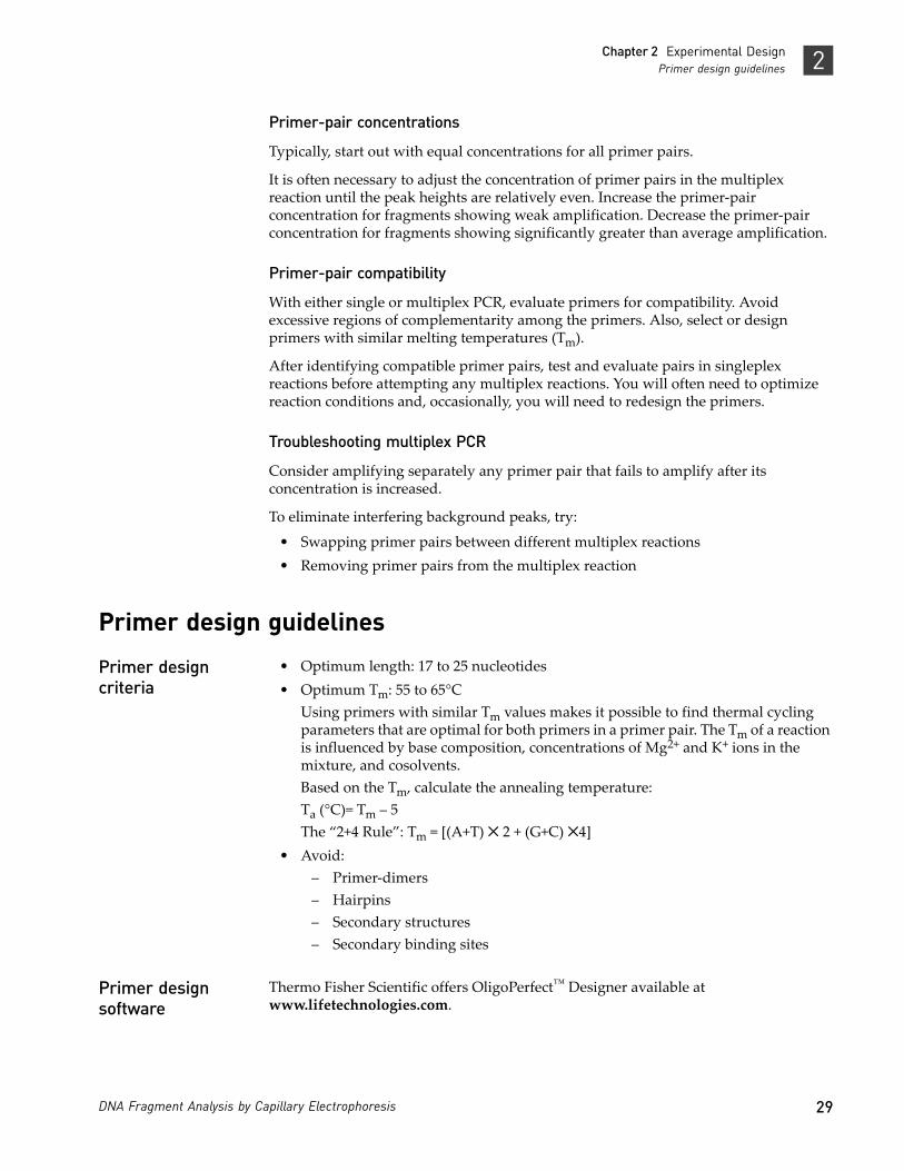
29DNA Fragment Analysis by Capillary Electrophoresis
Chapter 2 Experimental DesignPrimer design guidelines 2
Primer-pair concentrations
Typically, start out with equal concentrations for all primer pairs.
It is often necessary to adjust the concentration of primer pairs in the multiplex reaction until the peak heights are relatively even. Increase the primer‐pair concentration for fragments showing weak amplification. Decrease the primer‐pair concentration for fragments showing significantly greater than average amplification.
Primer-pair compatibility
With either single or multiplex PCR, evaluate primers for compatibility. Avoid excessive regions of complementarity among the primers. Also, select or design primers with similar melting temperatures (Tm).
After identifying compatible primer pairs, test and evaluate pairs in singleplex reactions before attempting any multiplex reactions. You will often need to optimize reaction conditions and, occasionally, you will need to redesign the primers.
Troubleshooting multiplex PCR
Consider amplifying separately any primer pair that fails to amplify after its concentration is increased.
To eliminate interfering background peaks, try:
• Swapping primer pairs between different multiplex reactions• Removing primer pairs from the multiplex reaction
Primer design guidelines
Primer design criteria
• Optimum length: 17 to 25 nucleotides• Optimum Tm: 55 to 65°C
Using primers with similar Tm values makes it possible to find thermal cycling parameters that are optimal for both primers in a primer pair. The Tm of a reaction is influenced by base composition, concentrations of Mg2+ and K+ ions in the mixture, and cosolvents.Based on the Tm, calculate the annealing temperature:Ta (°C)= Tm – 5 The “2+4 Rule”: Tm = [(A+T) ✕ 2 + (G+C) ✕4]
• Avoid:– Primer‐dimers – Hairpins – Secondary structures– Secondary binding sites
Primer design software
Thermo Fisher Scientific offers OligoPerfect™ Designer available at www.lifetechnologies.com.

30 DNA Fragment Analysis by Capillary Electrophoresis
Chapter 2 Experimental DesignPrimer design guidelines2
Factors affecting Tm and primer annealing
Primer annealing is influenced by:
• Primer/template base composition• Primer/template base order• Primer or template secondary structure
Effects of base composition
G‐C bonds contribute more to the stability (increased melting temperature) of primer/template binding than do A‐T bonds.
To ensure stable annealing of primer and template while avoiding problems with the internal secondary structure of primers or long stretches of any one base, select primers with a 40% to 60% G+C content.
Note: Designing primers based on Tm and primer length to avoid primer‐dimers and gapped‐duplex structures is more important than designing primers based on actual percent G+C content.
Effects of base order
Two primer/template complexes with identical content may have different Tm values because base order influences the overall annealing stability. You can determine the exact effect of base order on complex stability using the base‐pairing energies listed in Table 4 (adapted from Salser, 1978). Larger negative values represent more stable interactions between the template and primer.
Table 4 Base-pairing energies (kcal/dinucleotide pair)
Example: Consider the two sequences: 3‐GAC‐5ʹ and 3ʹ‐CGA‐5ʹ. The sequence 3‐GAC‐5ʹ contained within a primer would contribute – 4.2 kcal to the binding energy (– 2.1 kcal [3‐GA‐5ʹ] + – 2.1 kcal [3‐AC‐5ʹ] = – 4.2 kcal). However, if the G and C are next to each other, as in 3‐CGA‐5ʹ, the contribution increases to – 6.4 kcal (– 4.3 kcal [3‐CG‐5ʹ] + – 2.1 kcal [3‐GA‐5ʹ] = – 6.4 kcal).
Note: Although a G‐C dinucleotide at the 3ʹ end of the primer can stabilize the template‐primer binding complex when using thermostable enzymes such as AmpliTaq® DNA Polymerase, a 3ʹ G‐C can also lead to false priming if you do not optimize PCR conditions (Topal and Fresco, 1976).
Effects of primer secondary structure
Strings of Gs and Cs can form internal, non‐Watson‐Crick base pairs (Sarocchi et al., 1970) that disrupt stable primer annealing. Although this anomalous behavior is difficult to predict, a good general rule is to avoid runs of more than three consecutive Gs in primers.
5' Nucleotide 3' Nucleotide
A C G T
A –1.2 –2.1 –2.1 –1.8
C –2.1 –4.8 –3.0 –2.1
G –2.1 –4.3 –4.8 –2.1
T –1.8 –2.1 –2.1 –1.2

31DNA Fragment Analysis by Capillary Electrophoresis
Chapter 2 Experimental DesignPrimer design guidelines 2
However, a short run of Gs at or near the 5ʹ end of a primer will not disrupt the stability of primer‐template complexes because 5ʹ positioning does not lead to involvement in disruptive secondary structures (for example, primer‐dimer or duplex loops).
Similarly, self‐complementary sequences within the primer can lead to the formation of hairpin structures that disrupt stable primer binding to template. A stable hairpin can form with just four G+C base pairs in the stem and three bases in the loop (Summer et al., 1985) (Figure 4).
Figure 4 Secondary structures in primers
Effects of template secondary structure
Primers do not bind effectively to target sequences with known secondary structures. For example, hairpin structures are often found in regions of high G+C content or in RNA sequences. If you must design primers to a specific target region with the potential for hairpin formation, you may try addition of DMSO to your reaction or other commercially available kits for difficult template amplification.
Selective amplification
Amplification of the desired target sequence requires minimizing primer binding to secondary sites in the DNA and to other primers.
Note: This applies to template genomic DNA. The probability of binding to secondary sites is lower for low‐complexity templates, such as plasmid DNA.
Ideally, the binding of the primer to the desired template region:
• Is strongest at the 5ʹ end.• Generally requires a higher, more negative value (to maximize base‐pairing
energy) than – 9.8 kcal/mole at the 3ʹ end (see Table 4 on page 30).
As a general rule, binding at the 3’ end should be weaker than – 9.8 kcal/mole.
Preferential amplification
When alleles differ in size by ten or more base pairs you may observe preferential amplification of shorter PCR products over longer ones (Walsh et al., 1992). This will also occur when amplifying low copy‐number DNA or DNA isolated from paraffin‐embedded tissues. Figure 5 on page 32 is an example of preferential amplification of the D5S346 marker. In both the normal (top panel) and tumor (bottom panel) samples, the peak height of the larger 124‐base pair (bp) fragment is much lower than that of the smaller 110‐bp fragment.
Hairpin loop sequence
Multiple binding sites
Forward and reverse primers
Hairpin loop sequence
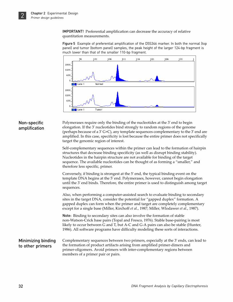
32 DNA Fragment Analysis by Capillary Electrophoresis
Chapter 2 Experimental DesignPrimer design guidelines2
IMPORTANT! Preferential amplification can decrease the accuracy of relative quantitation measurements.
Figure 5 Example of preferential amplification of the D5S346 marker. In both the normal (top panel) and tumor (bottom panel) samples, the peak height of the larger 124-bp fragment is much lower than that of the smaller 110-bp fragment.
Non-specific amplification
Polymerases require only the binding of the nucleotides at the 3ʹ end to begin elongation. If the 3ʹ nucleotides bind strongly to random regions of the genome (perhaps because of a 3ʹ G+C), any template sequences complementary to the 3ʹ end are amplified. In this case, specificity is lost because the entire primer does not specifically target the genomic region of interest.
Self‐complementary sequences within the primer can lead to the formation of hairpin structures that decrease binding specificity (as well as disrupt binding stability). Nucleotides in the hairpin structure are not available for binding of the target sequence. The available nucleotides can be thought of as forming a “smaller,” and therefore less specific, primer.
Conversely, if binding is strongest at the 5ʹ end, the typical binding event on the template DNA begins at the 5ʹ end. Polymerases, however, cannot begin elongation until the 3ʹ end binds. Therefore, the entire primer is used to distinguish among target sequences.
Also, when performing a computer‐assisted search to evaluate binding to secondary sites in the target DNA, consider the potential for “gapped duplex” formation. A gapped duplex can form when the primer and target are completely complementary except for a single base (Miller, Kirchoff et al., 1987; Miller, Wlodawer et al., 1987).
Note: Binding to secondary sites can also involve the formation of stable non‐Watson‐Crick base pairs (Topal and Fresco, 1976). Stable base‐pairing is most likely to occur between G and T, but A‐C and G‐A pairs can also be stable (Hunter, 1986). All software programs have difficulty modeling these sorts of interactions.
Minimizing binding to other primers
Complementary sequences between two primers, especially at the 3ʹ ends, can lead to the formation of product artifacts arising from amplified primer‐dimers and primer‐oligomers. Avoid primers with inter‐complementary regions between members of a primer pair or pairs.

33DNA Fragment Analysis by Capillary Electrophoresis
Chapter 2 Experimental DesignPrimer design guidelines 2
Post-amplification manipulations
Adding extensions that are not complementary to the template at the 5’ end of the primer can facilitate a variety of useful post‐amplification manipulations of the PCR product without adversely affecting yield. Examples include 5ʹ extensions that contain restriction sites, universal primer binding sites, or promoter sequences.
Addition of 3' A nucleotide by Taq polymerase
The AmpliTaq® and AmpliTaq Gold® DNA Polymerases, like many other DNA polymerases, catalyze the addition of a single nucleotide (usually an adenosine) to the 3ʹ ends of the two strands of a double‐stranded DNA fragment. This non‐template complementary addition results in a denatured PCR product that is one nucleotide longer than the target sequence. A PCR product containing the extra nucleotide is referred to as the plus‐A form.
Incomplete 3' A nucleotide addition
Because 3ʹ A nucleotide addition rarely goes to completion without a long extension step at the end of thermal cycling (that is, only a fraction of the fragments receive the extra nucleotide), single‐base ladders often form, creating peak patterns that analysis software might not interpret correctly (Figure 6). The resulting allele calls can be inconsistent, incorrect, or missing entirely.
Figure 6 Split peaks resulting from incomplete 3' A nucleotide addition

34 DNA Fragment Analysis by Capillary Electrophoresis
Chapter 2 Experimental DesignPrimer design guidelines2
Avoiding incomplete 3' A nucleotide addition
Modify Considerations
Thermal cycling conditions Increasing the time spent between 60 and 72°C promotes 3' A nucleotide addition. Decreasing the time spent between 60 and 72°C inhibits 3' A nucleotide addition.
To use this method effectively, determine the optimal thermal cycling conditions for each marker in each set of reaction conditions.
Promoting 3' A nucleotide addition has proven to be more successful than removing 3' A. Residual polymerase activity at room temperature (or even at 4°C) is often sufficient to catalyze enough 3' A nucleotide addition to create genotyping problems. Many protocols increase the final extension step to 30 to 45 minutes to promote 3' A nucleotide addition.
Magnesium ion concentration Increasing the magnesium ion concentration promotes 3' A nucleotide addition. Decreasing the magnesium ion concentration inhibits 3' A nucleotide.
In general, optimizing the magnesium ion concentration is best used in conjunction with other strategies. If you choose to maximize 3'A nucleotide addition, consider using AmpliTaq Gold® DNA Polymerase at 2.5 mM MgCI2.
“Tail”
the 5' end of the reverse primer
Brownstein et al. (1996) found that adding additional nucleotides (a “tail”) to the 5' end of the reverse PCR primer either promoted or inhibited 3' A nucleotide addition to the (forward) labeled strand, depending on the sequence of the added nucleotides (Figure 7 on page 35).
Magnuson et al. (1996) noticed a correlation between tail sequence and the amount of 3' A nucleotide addition. In particular, they found that adding a single G to the 5' end of the reverse PCR primer generally resulted in almost complete 3' A nucleotide addition. Therefore, using a tail to promote 3' A nucleotide addition can consistently yield a pattern that analysis software can identify.
Reverse-primer tailing has advantages compared to other methods because it:• Works well under diverse reaction conditions• Does not require additional experimental steps
Go to www.lifetechnologies.com for information on ordering tailed primers.

35DNA Fragment Analysis by Capillary Electrophoresis
Chapter 2 Experimental DesignPrimer design guidelines 2
Figure 7 Tailed primers and 3' A nucleotide addition
Note: In general, the most reliable strategy is to promote 3ʹ A nucleotide addition by modifying thermal cycling conditions and Mg2+ concentration, and (if necessary) by tailing the reverse primer.
Enzymatic treatment
Ginot et al. (1996) used T4 DNA polymerase to remove the 3ʹ A overhangs from treatment‐pooled PCR products.
Although effective, this method has serious limitations because it requires:
• A post‐PCR enzymatic treatment step• Titrating each lot of T4 DNA polymerase to determine optimal enzyme
concentrations and treatment times
IMPORTANT! Excess T4 treatment can cause PCR product degradation. Insufficient treatment will not remove the 3’ overhangs and can make some alleles more difficult to genotype.
Start optimization experiments with 0.5 to 1 unit of T4 DNA polymerase in 10 μL of pooled PCR product. Incubate at 37°C for 30 minutes.
Labeled primer
Tailed primerWithout tailed primers
With tailed primers (plus 7 bp)

36 DNA Fragment Analysis by Capillary Electrophoresis
Chapter 2 Experimental DesignDyes2
Dyes
IMPORTANT! We recommend using only Thermo Fisher Scientific dyes. Thermo Fisher Scientific provides spectral calibration reagents that have been optimized for our dye sets.
Other dyes (or mixed isomers of dyes) have variable emission spectra and also require a spectral calibration generated for the specific dyes in use to correct for the spectral overlap between the dyes. You are responsible for obtaining the appropriate spectral calibration reagents and for optimizing custom dye sets.
Dyes and chemical forms
Thermo Fisher Scientific dyes are available in multiple chemical forms. Some forms are supplied coupled to primers and others you can use to label custom primers or fragments. Each form has distinct advantages and disadvantages depending upon the intended application and your laboratory setup.
You can analyze phosphoramidite‐labeled fragments with NHS‐ester‐labeled fragments, but you should not combine [F]dNTP‐labeled fragments with any other labeling method.
Table 5 Dye chemical forms
Multicomponent analysis with fluorescent dyes
Fluorescent‐dye labeling enables you to analyze multiple independent markers (loci) in the same capillary injection by using different dye colors in addition to size to distinguish between markers.
During data collection on our genetic analyzers, the fluorescence signals are separated by diffraction grating according to wavelength and projected onto a CCD camera in a predictably spaced pattern.
Chemical form Purpose Available dyes
NHS-esters Post-synthesis 5'-end labeling of oligonucleotides containing a 5' Aminolink2
NED™†, TAMRA™‡, ROX™
SNaPshot® Kit dyes: dR110, dR6G, dTAMRA™‡, dROX™
Phosphoramidite reagents
Preparing custom, 5'-end labeled primers directly on any Thermo Fisher Scientific DNA synthesizer§
6-FAM™, HEX™, TET™, NED™†, VIC®†, PET®†
[F]dNTPs Simple internal fluorescent labeling of multiple nucleotides during PCR amplification
R6G, R110, ROX™, TAMRA™‡
Labeled primers in reagent kits
Microsatellite and human identification applications 5-FAM™††, JOE™††, 6-FAM™, HEX™, TET™, NED™†, VIC®†, PET®†
Labeled size standard
Generating the sizing curve to size unknown sample fragments TAMRA™‡, ROX™, LIZ®
† NED™, VIC®, and PET dye-labeled primers are available only in kits or through the Thermo Fisher Scientific Custom Oligo Service. Contact your Thermo Fisher Scientific representative or visit our website for information on how to order custom-labeled oligonucleotides.
‡ Matrix standards for spectral calibration available for the 310 instrument only.§ For information about synthesizing labeled oligonucleotides, contact your Thermo Fisher Scientific representative.††5-FAM™ and JOE™ are available only as labeled primers in certain reagent kits.

37DNA Fragment Analysis by Capillary Electrophoresis
Chapter 2 Experimental DesignDyes 2
Although each dye emits its maximum fluorescence at a different wavelength, there is some overlap in the emission spectra between the dyes (Figure 8). To correct for spectral overlap, the software applies a multicomponent matrix. A multicomponent matrix is created when you perform a spectral calibration for a dye set using a matrix standard (for more information, see “Dye sets” on page 41 and “Understanding spectral calibration” on page 84).
Figure 8 Emission spectra of dyes
Factors that affect dye signal
Fluorescent dyes have the following characteristics:
• Emission spectrum: The intensity of emitted light (fluorescence) as a function of the wavelength of the emitted light.
• Absorption (excitation) spectrum: The intensity of emitted light as a function of the wavelength of the exciting light.
• Absorption (excitation) efficiency: A measure of the probability that a dye will absorb light of a certain wavelength, as a percentage of the probability of absorption at the wavelength of maximum absorption.
• Quantum yield: The probability that its excited state will emit a photon as it decays back to the ground state.
The ability of the instrument to detect a dye signal depends upon:
• The absorption efficiency of the dye at the wavelengths of light emitted by the laser
• The laser/light source • The quantum yield of the dye• The dye concentration
The emission and absorption wavelengths of a dye depend upon:
• The chemical structure of the dye• The physical environment, including:
– Buffer pH and concentration – Polymer composition– Whether the DNA it is attached to is single‐ or double‐stranded
Although altered by the physical environment, the wavelengths of maximum emission and absorption for each dye always lie within a small wavelength range.
Nor
mal
ized
Em
issi
on
Wavelength (nm)
Dyes6-FAM PETNEDVIC LIZ
0
20
40
60
80
100
500 550 600 650 700

38 DNA Fragment Analysis by Capillary Electrophoresis
Chapter 2 Experimental DesignDyes2
Emission and absorption (excitation) wavelengths and relative intensities
The maximum fluorescence absorption and emission wavelengths are listed below for Thermo Fisher Scientific NHS‐esters, dye phosphoramidites, and [F]dNTP‐based dyes. (The actual maximum absorption and emission wavelengths may differ from the listed values because of the influence of the physical environment upon the dye.)
The intensity of emitted fluorescence is different for each dye, and you must optimize sample concentration to account for differences in dye signal strength.
Examples:
• 6‐FAM™dye emits a stronger signal than NED™dye. Therefore, to generate signals of equal intensity, you must load approximately three times as much NED™ dye‐labeled fragments as 6‐FAM™dye‐labeled fragments.
• VIC® dye emits a stronger signal and is more stable than HEX™ dye. Use VIC® dye for weak amplicons.
Table 6 Dye Absorption max, emission max, and relative intensities
Dye Absorption Max Emission Max Relative Intensity
Intensity (not to scale)
5-FAM™ 494 nm 530 nm 100 RFU
6-FAM™ 494 nm 522 nm 100 RFU
TET™ (310 only)
521 nm 538 nm 100 RFU
VIC® 538 nm 554 nm 100 RFU
JOE™ 528 nm 554 nm 50 RFU
HEX™ 535 nm 553 nm 50 RFU
LIZ® 638 nm 655 nm 50 RFU
NED™ 546 nm 575 nm 40 RFU
TAMRA™ 560 nm 583 nm 25 RFU
ROX™ 587 nm 607 nm 25 RFU
PET® 558 nm 595 nm 25 RFU

39DNA Fragment Analysis by Capillary Electrophoresis
Chapter 2 Experimental DesignDyes 2
Points to consider when selecting dyes for custom primers
When you order custom primers, you specify the dyes for labeling. Based on the dyes you specify, you must use the appropriate dye set to perform a spectral calibration (described in “Dye sets” on page 41).
Consider the following when selecting dyes:
• One dye is needed for the size standard (red or orange).• Using 5 dyes provides 33% greater throughput than using 4 dyes.• Use the most intense dyes for PCR products with low recovery rate (from lower to
higher intensity: Blue > Green > Yellow > Red) (see “Emission and absorption (excitation) wavelengths and relative intensities” on page 38).
• Use less‐intense dyes for PCR product with good recovery rate.• Select dyes with absorption maxima that are as far apart as possible to avoid
overlap and for easier generation of matrix/spectral calibration (see “Emission and absorption (excitation) wavelengths and relative intensities” on page 38).
• Consider the relative dye intensities and sample concentration (see “Emission and absorption (excitation) wavelengths and relative intensities” on page 38).
Example: selecting dyes
The following figure shows the marker range (allele distribution) and allele frequencies for the alligator microsatellite locus Amiμ‐8 for samples taken from Florida/South Georgia and Texas/Louisiana.
Figure 9 Allele distribution for alligator marker Amiµ-8 in two populations (124 to 156 bp)
Using a hypothetical set of 10 markers as an example:
• For each marker, determine the expected allele distribution, either from published literature or from empirical testing.
• Determine the dyes that are appropriate for the range of each marker of interest.

40 DNA Fragment Analysis by Capillary Electrophoresis
Chapter 2 Experimental DesignDyes2
• For this hypothetical set of markers, you might select 6‐FAM™, VIC®, PET®, NED™ dyes, and LIZ® dye for the size standard (see the table below). This group of dyes corresponds to the G5 dye set, so you would also need the DS‐33 matrix standard for spectral calibration (see Table 7 on page 41 for the matrix standard that corresponds to each dye set).Note that different dyes can be used for similar fragment lengths, and the same dye can be used for fragments of different lengths.
Locus Marker Range Dye Capillary electrophoresis array view
of example 10-marker panel
Marker 1 90–104 6-FAM™
Marker 2 112–146 VIC®
Marker 3 119–177 PET®
Marker 4 117–202 NED™
Marker 5 156–190 6-FAM™
Marker 6 221–253 6-FAM™
Marker 7 234–282 NED™
Marker 8 260–342 VIC®
Marker 9 311–327 6-FAM™
Marker10 340–380 NED™

41DNA Fragment Analysis by Capillary Electrophoresis
Chapter 2 Experimental DesignDye sets 2
Dye sets
Dye sets and matrix standards
A dye set corresponds to the group of dyes you select for labeling (described in the previous section). You use the matrix standard that corresponds to the dye set (shown below) to perform a spectral calibration. This calibration prepares the instrument for detection of the dyes with which your primers are labeled. For information on spectral calibration, see “Understanding spectral calibration” on page 84.
Table 7 Dye set and matrix standard components
The kits available from Thermo Fisher Scientific use the dye sets listed below.
Table 8 Dye sets and matrix standards for kits and genotyping applications
Creating a custom dye set
IMPORTANT! We recommend using only Thermo Fisher Scientific dyes. Thermo Fisher Scientific provides spectral calibration reagents that have been optimized for our dye sets.
Non‐Thermo Fisher Scientific dyes (or mixed isomers of dyes) have variable emission spectra and also require a spectral calibration generated for the specific dyes in use to correct for the spectral overlap between the dyes. You are responsible for obtaining the appropriate spectral calibration reagents and for optimizing custom dye sets to ensure the dye labels do not affect PCR efficiency.
Dye Set
(ROX™, LIZ®, and TAMRA™ dyes are reserved for the size standard)
Dye Set E5 D D F G5 C†
† Used on 310 instruments only.
Matrix standard DS-02 DS-30‡§
‡ Can be used for custom-labeling primers.§ DS-30 versus DS-31: VIC® dye emits a stronger signal and is more stable than HEX™ dye. Use VIC® dye for
weak amplicons.
DS-31§ DS-32 DS-33§ DS-34
Blue dR110 6-FAM™ 6-FAM™ 5-FAM™ 6-FAM™ 6-FAM™
Green dR6G HEX™ VIC® JOE™ VIC® TET™
Yellow dTAMRA™ NED™ NED™ NED™ NED™ HEX™
Red dROX™ ROX™ ROX™ ROX™ PET® TAMRA™
Orange LIZ® — — — LIZ® —
Application Dye Set Matrix Standard
SNaPshot® Primer Focus®, SNaPshot® Multiplex E5 DS-02
Custom oligos D DS-30
Custom oligos, Plant and Microbial AFLP®, Bovine and Canine Stockmarks®
D DS-31
Stockmarks®, AFLP® F DS-32
Equine Stockmarks®, custom oligos, AmpFlSTR® G5 DS-33

42 DNA Fragment Analysis by Capillary Electrophoresis
Chapter 2 Experimental DesignSize standards2
However, the 3500 Series, 3730 Series, and 3130 Series instruments do support custom dye sets. For information, see Chapter 4, “Optimizing Capillary Electrophoresis” on page 67.
Size standards
Functions of a size standard
Each unknown sample is mixed with size standard before electrophoresis and run together in the same capillary with the same conditions. Size standards perform two functions:
• Allow sizing of sample peaks. A size curve is generated for each sample. Because the sizes (in bp) of the size‐standard peaks are known, the sizes of sample peaks are determined through a relative comparison of migration speeds during electrophoresis. The uniform spacing of size‐standard fragments ensures precise sizing throughout the sizing range.
IMPORTANT! Because the called size for a fragment can differ from its actual size, compare the allele calls instead of the fragment size.
IMPORTANT! Use the same size standard, instruments, and instrument conditions for all samples in a study. Using different size standards, instruments, or instrument conditions may shift the sizing of DNA fragments.
Precision, or reproducibility, is the measure of instrument ability to generate the same size consistently for a given fragment.For more information, see “Precise versus accurate sizing” on page 90, “Guidelines for consistent sizing” on page 90, and “How the GeneMapper® Software performs sizing” on page 98.
• Correct for injection‐to‐injection variations that result in differences when comparing the same DNA fragments from different capillaries, runs, and instruments. When comparing fragment size across injections, ensure that data is analyzed with the same sizing method and the same size‐standard definition.
Size-standard peak intensity
For optimum performance, the signal intensity of the size‐standard peaks should be lower than or equal to the signal intensity of the sample peaks. For more information, see “Balancing size‐standard and sample‐peak intensities” on page 77.

43DNA Fragment Analysis by Capillary Electrophoresis
Chapter 2 Experimental DesignSize standards 2
Selecting a GeneScan™ size standard
Select a size standard with at least two fragments smaller and larger than your unknown sample fragments, and with a dye that is compatible with the dyes used for labeling primers.
Peaks not used for sizing
Some size standards include peaks that are not used for sizing. These peaks are denoted with a “*” in the following figures. These peaks can be used as an indicator of precision within a run.
Preparing a size standard
1. Vortex to mix the contents of each size‐standard tube thoroughly, then centrifuge briefly to collect the liquid at the bottom of the tube.
2. Optimize the ratio of sample‐to‐size standard and Hi‐Di™ formamide using the values listed below as a starting point.
3. Create a master mix of the size standard and formamide.
4. Add samples and master mix to tubes or wells.
5. Heat the reaction mix for 3 to 5 minutes at 95°C. Immediately chill on ice for 2 to 3 minutes, then load samples.
IMPORTANT! After size standards are mixed with formamide, run immediately. Signal will decrease significantly if left at room temperature for >1 day or at 2 to 8°C for >5 days. Plates can be stored at –20°C for up to 1 week.
Expected marker length
LIZ® Size Standard, 5-dye chemistry ROX™ Size Standard, 4-dye chemistry
GS120 LIZ®†
(page 47)
GS500 LIZ®‡
(page 50)
GS600 LIZ®‡
(page 45)
GS1200 LIZ®‡
(page 47)
GS350 ROX™
(page 49)
GS400HD ROX™
(page 49)
GS500 ROX™‡
(page 50)
GS1000 ROX™
(page 51)
≤ 120 bp ✓ — — — ✓ — — —
≤ 400 bp — ✓ ✓ — ✓ ✓ ✓ —
≤ 500 bp — ✓ ✓ — — — ✓ ✓
≤ 600 bp — — ✓ — — — — —
≤ 1000 bp — — — — — — — ✓
≤ 1200 bp — — — ✓ — — — —
† Used with SNaPshot® Multiplex Kit.‡ For denaturing and non-denaturing applications.
Components 3500 Series, 3730 Series, and 3130 Series instruments 310 instrument
Sample 0.5 µL per reaction 0.5 µL per reaction
Size standard 0.5 µL per reaction 0.5 µL per reaction
Hi-Di™ Formamide†
† Hi-Di™ Formamide (Part no. 4311320) is purchased separately from the size standard.
9.0 µL per reaction 11.0 µL per reaction

44 DNA Fragment Analysis by Capillary Electrophoresis
Chapter 2 Experimental DesignSize standards2
GeneScan™ 120 LIZ® Size Standard
Range: 15 to 120 bp under denaturing conditions
This single‐stranded size standard was designed to provide accurate sizing of short DNA fragments. Therefore, it is particularly useful for SNP analysis. All fragments have been optimized under a wide variety of run conditions.
Figure 10 GeneScan™ 120 Size Standard run under denaturing conditions
GeneScan™ 500 LIZ® Size Standard
Range: 35 to 500 bp under denaturing conditions
This size standard is recommended for analysis of tri‐ and tetranucleotide microsatellite loci, which can often exceed 400 bp in length.
Only one strand of the double‐stranded DNA fragments in this size standard is labeled. The unlabeled strand does not interfere with peak detection of the labeled strand when run under denaturing conditions.
GeneScan™ 120 LIZ® denatured fragment lengths (nt): 9 fragments
15 35 80
20 50 110
25 62 120
GeneScan™ 500 LIZ® denatured fragment lengths (nt): 16 fragments
35 139 250†
† Do not use this fragment for sizing. See “Peaks not used for sizing” on page 43 for information.
400
50 150 300 450
75 160 340 490
100 200 350 500

45DNA Fragment Analysis by Capillary Electrophoresis
Chapter 2 Experimental DesignSize standards 2
Figure 11 GeneScan™ 500 LIZ® Size Standard run under denaturing conditions
GeneScan™ 600 LIZ® and GeneScan™ 600 LIZ® v2.0 Size Standards
Note: The GeneScan™ 600 LIZ® and GeneScan™ 600 LIZ® v2.0 Size Standards contain the same peaks. The GeneScan™ 600 LIZ® v2.0 Size Standard can be used for normalization on 3500 Series instruments.
Range: 20 to 600 bp under denaturing conditions
GeneScan™ 600 LIZ® denatured fragment lengths (nt): 36 fragments
20 120 220 314 414 514
40 140 240 320 420 520
60 160 250 340 440 540
80 180 260 360 460 560
100 200 280 380 480 580
114 214 300 400 500 600

46 DNA Fragment Analysis by Capillary Electrophoresis
Chapter 2 Experimental DesignSize standards2
Figure 12 GeneScan™ 600 LIZ® Size Standard fragments run under denaturing conditions
Optimizing the 3130 Series instrument run module
The run modules provided with these instruments may need to be optimized for use with the GeneScan™ 600 LIZ® Size Standard. Add 100 seconds to the run time if needed.
Optimizing the 310 instrument run module
The run modules provided with these instruments have not been optimized for use with the GeneScan™ 600 LIZ® Size Standard. Add 200 seconds to the run time before using this size standard.

47DNA Fragment Analysis by Capillary Electrophoresis
Chapter 2 Experimental DesignSize standards 2
GeneScan™ 1200 LIZ® Size Standard
Range: 20 to 1200 bp under denaturing conditions
The high fragment density (68 fragments) yields greater sizing precision, and landmark fragments allow easy peak‐pattern identification during data analysis.
This size standard is ideal for BAC fingerprinting, T‐RFLP, VNTR, STR, and many other DNA fragment analysis applications.
Figure 13 GeneScan™ 1200 LIZ® Size Standard run under denaturing conditions
GeneScan™ 1200 LIZ® Size Standard denatured fragment lengths (nt): 68 fragments
20 280 560 850
30 300 580 860
40 314 600 880
60 320 614 900
80 340 620 920
100 360 640 940
114 380 660 960
120 400 680 980
140 414 700 1000
160 420 714 1020
180 440 720 1040
200 460 740 1060
214 480 760 1080
220 500 780 1100
240 514 800 1120
250 520 820 1160
260 540 840 1200

48 DNA Fragment Analysis by Capillary Electrophoresis
Chapter 2 Experimental DesignSize standards2
Downloading 3130 instrument run modules from our website
Updated run modules for the 3130 Series instrument and the GeneScan™ 1200 LIZ® Size Standard are available on our website. Before using the downloaded run modules, adjust as described below. Further optimization may be necessary.
Downloading 3730 instrument run modules from our website
Updated run modules for the 3730 Series instrument and the GeneScan™ 1200 LIZ® Size Standard are available on our website. Before using the downloaded run modules, adjust as described below. Further optimization may be necessary.
36-cm array with POP-4® polymer 50-cm array with POP-4® polymer
• Decrease run voltage to 8000 volts• Increase run time to 6000 seconds
• Decrease run voltage to 12,000 volts• Increase run time to 6000 seconds
50-cm array
• Decrease run voltage to 8000 volts• Increase run time to 6200 seconds

49DNA Fragment Analysis by Capillary Electrophoresis
Chapter 2 Experimental DesignSize standards 2
GeneScan™ 350 ROX™ Size Standard
Range: 35 to 350 bp under denaturing conditions
Only one strand of the double‐stranded DNA fragments in this size standard is labeled. The unlabeled strand does not interfere with peak detection of the labeled strand when run under denaturing conditions.
Figure 14 GeneScan™ 350 Size Standard run under denaturing conditions
GeneScan™ 400HD ROX™ Size Standard
This size standard uses ROX™ dye. The high density of marker bands in this standard makes it particularly useful for microsatellite analysis.
Range: 50 to 400 bp under denaturing conditions
Only one strand of the double‐stranded DNA fragments in this size standard is labeled. The unlabeled strand does not interfere with peak detection of the labeled strand.
GeneScan™ ROX™ 350 denatured fragment lengths (nt): 12 fragments
35 139 250†
† Do not use this fragment for sizing. See “Peaks not used for sizing” on page 43 for information.
50 150 300
75 160 340
100 200 350
*
100
30020
0160
150
139
350
340
75
35 50
GeneScan™ ROX™ 400HD denatured fragment lengths (nt): 21 fragments
50 160 260 360
60 180 280 380
90 190 290 400
100 200 300 —
120 220 320 —
150 240 340 —

50 DNA Fragment Analysis by Capillary Electrophoresis
Chapter 2 Experimental DesignSize standards2
Figure 15 GeneScan™ 400HD Size Standard run under denaturing conditions
GeneScan™ 500 ROX™ Size Standard
Range: 35 to 500 bp under denaturing conditions
This size standard is recommended for analysis of tri‐ and tetranucleotide microsatellite loci, which can often exceed 400 bp in length.
Only one strand of the double‐stranded DNA fragments in this size standard is labeled. The unlabeled strand does not interfere with peak detection of the labeled strand when run under denaturing conditions.
GeneScan™ 500 ROX™ denatured fragment lengths (nt): 16 fragments
35 139 250†
† Do not use this fragment for sizing. See “Peaks not used for sizing” on page 43 for information.
400
50 150 300 450
75 160 340 490
100 200 350 500

51DNA Fragment Analysis by Capillary Electrophoresis
Chapter 2 Experimental DesignSize standards 2
Figure 16 GeneScan™ 500 ROX™ Size Standard run under denaturing conditions
GeneScan™ 1000 ROX™ Size Standard
Range:
• 100 to 900 bp under non‐denaturing conditions• 100 to 539 bp under denaturing conditions (verified with POP‐4® polymer only)
Both strands of the GeneScan™ 1000 ROX™ Size Standard fragments are labeled and are used for non‐denaturing applications.
GeneScan™ 1000 ROX™ non-denatured fragment lengths† (nt): 17 fragments
† If run under denaturing conditions (Figure 17 on page 52), fragments run 18 nucleotides shorter than the lengths listed above and some or all of the peaks appear split.
47 93 292 695
51 99 317 946
55 126 439 —
82 136 557 —
85 262‡
‡ Do not use this fragment for sizing. See “Peaks not used for sizing” on page 43 for information.
692‡ —

52 DNA Fragment Analysis by Capillary Electrophoresis
Chapter 2 Experimental DesignOrdering custom primers2
Figure 17 GeneScan™ 1000 ROX™ Size Standard run under denaturing conditions. Fragments run 18 nt shorter than lengths obtained under non-denaturing conditions (see the table on the previous page). Under denaturing conditions, sizing is not accurate above 539 nt, therefore the and 674-nt (corresponds to the 692-nt) peak is not shown in the figure.
Note: Under denaturing conditions, the two strands of this doubly labeled size‐standard migrate at different rates, appearing as split peaks. To ensure sizing precision and a reliable size‐standard definition, you must define one peak from each split peak pair in the size‐standard definition.
Ordering custom primers
You can obtain custom 5ʹ‐end labeled primers from the Thermo Fisher Scientific Custom Oligo Service. For information, see our website.
Order labeled and unlabeled primer pairs for the markers of interest.
Testing the primers and optimizing conditions with test DNA panel
Testing Before using primers in an analysis, test the primers and optimize sample preparation, PCR, and electrophoresis conditions.
Create a panel of test DNA samples to ensure that expected alleles are detected for each marker. Use DNA samples that are representative of your overall study to capture as much allelic variation as possible. CEPH Individual 1347‐02 Control DNA is available from Thermo Fisher Scientific and can be used in your test DNA panel.
Test DNA panel guidelines:
• Include 8 to 16 samples• Use samples of good quality that are well‐quantified• Use equal concentrations of DNA samples
Note: If optimization of signal intensity is necessary for a given sample, inject the sample multiple times using a range of injection parameters.
*

53DNA Fragment Analysis by Capillary Electrophoresis
Chapter 2 Experimental DesignTesting the primers and optimizing conditions with test DNA panel 2
Order unlabeled primers for the markers of interest and optimize amplification conditions on your DNA test panel. You may need to optimize a variety of parameters including annealing temperature, and variables such as magnesium concentration and primer concentration to ensure that the primers work under universal conditions. Bands are visualized on agarose gels with ethidium bromide staining.
Optimizing conditions
The intensity of emitted fluorescence is different for each dye, and you must optimize sample concentration to account for differences in dye‐signal strength. For example, to generate signals of equal intensity, you must load approximately three times as much NED™ dye‐labeled fragments as 6‐FAM™dye‐labeled fragments.
For more information, see:
• Chapter 3, “Optimizing PCR” on page 55• Chapter 4, “Optimizing Capillary Electrophoresis” on page 67

54 DNA Fragment Analysis by Capillary Electrophoresis
Chapter 2 Experimental DesignTesting the primers and optimizing conditions with test DNA panel2

55DNA Fragment Analysis by Capillary Electrophoresis
3 Optimizing PCR
This chapter contains general information for PCR. For application‐specific information on PCR, see the application chapters later in this guide.
This chapter covers:
■ Safety information . . . . . . . . . . . . . . . . . . . . . . . . . . . . . . . . . . . . . . . . . . . . . . . . . . . . 55
■ Isolating, purifying, quantifying, and storing DNA . . . . . . . . . . . . . . . . . . . . . . . . 55
■ Handling primers . . . . . . . . . . . . . . . . . . . . . . . . . . . . . . . . . . . . . . . . . . . . . . . . . . . . . 57
■ Using control DNA. . . . . . . . . . . . . . . . . . . . . . . . . . . . . . . . . . . . . . . . . . . . . . . . . . . . 57
■ Reaction volumes and plate types . . . . . . . . . . . . . . . . . . . . . . . . . . . . . . . . . . . . . . . 58
■ Reagent concentrations . . . . . . . . . . . . . . . . . . . . . . . . . . . . . . . . . . . . . . . . . . . . . . . . 59
■ Preventing competing side reactions: hot‐start PCR. . . . . . . . . . . . . . . . . . . . . . . . 60
■ Thermal cycling parameters Veriti® Thermal Cyclers . . . . . . . . . . . . . . . . . . . . . . 60
■ Thermal cycling parameters 9700 Thermal Cyclers . . . . . . . . . . . . . . . . . . . . . . . . 62
■ Optimizing thermal cycling parameters . . . . . . . . . . . . . . . . . . . . . . . . . . . . . . . . . . 63
■ Avoiding contamination . . . . . . . . . . . . . . . . . . . . . . . . . . . . . . . . . . . . . . . . . . . . . . . 64
Safety information
IMPORTANT! For every chemical, read the Safety Data Sheets (SDSs) and follow the handling instructions. Wear appropriate protective eyewear, clothing, and gloves.
Note: For the SDSs of chemicals not distributed by Thermo Fisher Scientific, contact the chemical manufacturer.
Isolating, purifying, quantifying, and storing DNA
Isolating DNA DNA isolation methods depend on your starting DNA source. Refer to guidelines for your application for information on isolating DNA.
IMPORTANT! DO NOT FREEZE BLOOD SAMPLES before DNA isolation. Freezing can lyse red blood cells, and increase the concentration of PCR inhibitors in DNA samples.

56 DNA Fragment Analysis by Capillary Electrophoresis
Chapter 3 Optimizing PCRIsolating, purifying, quantifying, and storing DNA3
Purifying DNA The quality, accuracy, and amplified length of a DNA fragment can be significantly affected by characteristics of the sample itself and the method used for purification.
IMPORTANT! The success of AFLP® analysis is particularly dependent upon the quality of DNA.
Select a method based on the sample source or tissue type, how it was obtained from its source, and how it was handled or stored before purification. Go to www.lifetechnologies.com for the latest information on DNA purification.
Quantifying DNA For PCR with custom primers, optimize DNA concentration for your application. Concentration may range from 10 to 100 ng of purified DNA per reaction.
It is almost always necessary to dilute PCR amplification products before adding them to the sample tube. Typically, the required dilution is 1:3 to 1:80 (PCR product‐to‐distilled, deionized water or Hi‐Di™ Formamide).
Begin by optimizing PCR run conditions for your specific application. Then run a dilution series on your instrument to determine the optimal dilution. Alternatively, run 1 μL of PCR product on a mini‐gel. If, after ethidium bromide staining, the product signal is visible but not oversaturated, try a 1:10 dilution.
After determining the optimal dilution ratio, you can use the same dilutions for subsequent analyses because PCR yields should be fairly consistent. Any changes to the PCR conditions or the primer design may require different dilutions.
Note: Different dyes emit different fluorescent intensities. Therefore, PCR product concentrations may need optimization depending on relative fluorescence intensity during electrophoresis. See “Emission and absorption (excitation) wavelengths and relative intensities” on page 38.
Storing prepared DNA before or after PCR
Store the prepared samples at –20 °C to 4 °C until you perform capillary electrophoresis.

57DNA Fragment Analysis by Capillary Electrophoresis
Chapter 3 Optimizing PCRHandling primers 3
Handling primers
Reconstituting and diluting primers
Primers are commonly shipped in a lyophilized state. The units of a lyophilized primer are given as a mass, in picomoles.
To create a stock of primers or probe, reconstitute the primer or probe in sterile 1✕ TE buffer (1mM Tris, 0.1mM EDTA, pH 8.0) or sterile, nuclease‐free water.
Quantifying primers
Measure the primer quantity with a spectrophotometer using a primer‐specific absorption coefficient.
Storing primers • –20°C to –80°C for stock solution (undiluted, keep concentration as high as possible)
• +4°C for working solution, diluted appropriately (up to one month)
Using control DNA
Purpose of control DNA
• Serves as a positive control for troubleshooting PCR amplificationControl DNA allows you to distinguish between problems with the sample DNA (the control DNA amplifies but samples do not) and problems with reagents, thermal cyclers, or protocols (the control DNA does not amplify).
• Allows you to monitor sizing precisionBecause the control DNA is not used to calculate the sizing curve, you can use the sizes obtained during different capillary injections to verify that sizing precision (reproducibility) is within acceptable limits.
• Allows you to correlate the fragment sizes that are obtained in different runs or on different instruments.
Guidelines for use • Amplify at least one control DNA sample in every PCR run.• Include at least one injection of amplified control DNA during every series of
capillary runs. Use one control injection for every variation in the electrophoresis parameters.
CEPH 1347-02 Control DNA
CEPH Individual 1347‐02 Control DNA is available for human studies from Thermo Fisher Scientific (Part no. 403062).

58 DNA Fragment Analysis by Capillary Electrophoresis
Chapter 3 Optimizing PCRReaction volumes and plate types3
Reaction volumes and plate types
Reaction volumes Reaction volumes for Thermo Fisher Scientific PCR thermal cyclers are 5 to 100 μL.
Using small amounts of template
Although reaction tubes usually do not need to be sterilized or siliconized, use autoclaved tubes when amplifying with quantities (approximately 150 to 500 pg) of starting DNA template.
Autoclaved PCR tubes are available from Thermo Fisher Scientific (see “Thermal cyclers and accessories” on page 193).
Plate types Table 9 Reaction plates for each thermal cycler
Thermal Cycler Block Format Reaction Plate Type Networking capability Uses
Veriti® 96-Well Thermal Cycler
0.1 mL or 0.2 mL Alloy VeriFlex™ Blocks
Standard 0.2 mL and Fast 0.1 mL 96-well formats
Yes 10 to 80 μL medium/high throughput.
VeriFlex Blocks™ provide “better than gradient” PCR optimization.
Veriti® 384-Well Thermal Cycler
0.02 mL aluminum single block
384-well plate Yes 5 to 20 μL high throughput, small sample volume.
Dual 96-Well GeneAmp® PCR System 9700
2 aluminum 0.2 mL 96-well blocks
96-well, 0.2 mL format No 10 to 100 μL high throughput, small sample volume.
Dual 384-Well GeneAmp® PCR System 9700
2 aluminum 0.02 mL 384-well blocks
384-well, 0.02 mL format No 5 to 20 μL high throughput, small sample volume.
Auto-Lid Dual 384- Well GeneAmp® PCR System 9700
2 aluminum 0.02 mL 384-well blocks
384-well plate No 5 to 20 μL high throughput, small sample volume with robotic capability.
2720 Thermal Cycler
0.2 mL aluminum single block
96-well, 0.2 mL format No Ideal for basic PCR using 0.2 mL reaction tubes or 96-well reaction plates.

59DNA Fragment Analysis by Capillary Electrophoresis
Chapter 3 Optimizing PCRReagent concentrations 3
Reagent concentrations
The following factors can affect overall yield of specific DNA target sequences:
• dNTP concentration• Magnesium ion concentration• Primer concentration• Template concentration• Enzyme concentration
dNTP concentration
In the standard GeneAmp® PCR protocol, the concentration of each deoxynucleoside triphosphate (dNTP) is 200 μM.
In most cases, lower dNTP concentrations do not significantly affect the yield of PCR amplification product and will increase the fidelity of the PCR amplification product. However, for efficient base incorporation, keep the four dNTP concentrations balanced and above the estimated Km of each dNTP (10 to 15 μM).
Some applications might require higher dNTP concentration (especially when dNTP analogues are used). However, excess dNTPs decrease enzyme fidelity.
Magnesium ion DNA polymerases require free magnesium ion in solution for activity. For most PCR amplifications, you can relate product yield and specificity as well as enzyme fidelity to the free magnesium ion (Mg2+) concentration:
[free Mg2+] = [total Mg2+] ‐ [total dNTP] ‐ 2[EDTA]
In general, an increase in free magnesium concentration leads to an increase in product yield but a decrease in specificity and fidelity. To identify the magnesium concentration that gives the best compromise between yield and specificity, in the presence of 800 μM total dNTP concentration, run a MgCI2 reaction series in 50‐μM increments over the range from 100 to 400 μM MgCI2.
Template concentration
The concentration of template in a sample can affect the success of PCR amplification. Too much template promotes non‐specific binding of primers to secondary sites or changes the pH of the reaction mix. Too little template can result in poor yields, especially if the template is degraded.
Even very low template concentrations (10 copies) are often sufficient for successful PCR amplification.
If the starting sample is DNA, you can use up to 20,000 copies of the target to start optimization experiments. In general, this translates to:
• 1 to 5 ng of cloned template• 200 pg to 1 ng of genomic DNA
Start optimization experiments with less genomic DNA if starting sample is limited. With clean, good‐quality genomic DNA, 500 to 1000 pg of starting sample is typically sufficient.

60 DNA Fragment Analysis by Capillary Electrophoresis
Chapter 3 Optimizing PCRPreventing competing side reactions: hot-start PCR3
Enzyme concentration
For most PCR applications, 2.0 to 2.5 units of AmpliTaq Gold® DNA Polymerase is recommended for each 100‐μL reaction volume.
Note: To avoid the inaccuracies involved in pipetting 0.5‐μL amounts of enzyme into each reaction, prepare a fresh master mix of reagents and add the enzyme.
Preventing competing side reactions: hot-start PCR
When to use Consider using the hot‐start technique whenever you need to improve the specificity and sensitivity of your PCR amplifications. Loss of specificity and sensitivity are often caused by competing side reactions, which usually occur during the pre‐PCR setup period. (A common competing side reaction involves the amplification of non‐target sequences in background DNA due to mispriming or to primer oligomerization.)
Limitations and alternatives
The hot‐start technique is cumbersome. If you have high‐throughput needs, switching to AmpliTaq Gold® DNA Polymerase will give the same benefits as performing the hot‐start technique, without the need for using wax barriers or opening reaction tubes. If you are already using AmpliTaq Gold® DNA Polymerase, performing the hot‐start technique will not improve the specificity and sensitivity of PCR amplification.
Components necessary for amplification must be kept separately so that critical reactants do not mix until reaching a temperature sufficiently high to suppress primer self‐annealing or annealing to non‐target sequences.
Note: Although manual hot‐start PCR can increase specificity and yield, it is inconvenient and you can encounter reproducibility and contamination problems.
Thermal cycling parameters Veriti® Thermal Cyclers
AmpliTaq_Gold Use this profile for hot‐start PCR in place of labor‐intensive methods such as manual hot‐start or wax‐bead‐mediated hot‐start techniques. The Hot‐start technique helps to minimize the formation of primer‐dimers or non‐specific products, thereby increasing specificity and sensitivity of PCR. This profile specifies a pre‐PCR heat step for activation of AmpliTaq Gold® DNA Polymerase.

61DNA Fragment Analysis by Capillary Electrophoresis
Chapter 3 Optimizing PCRThermal cycling parameters Veriti® Thermal Cyclers 3
General PCR Use this profile for standard PCR.
Time-release PCR Use this profile with AmpliTaq Gold® DNA Polymerase. This method minimizes the pre‐PCR activation step and adds a minimum of 10 additional cycles, allowing for slow activation of the enzyme during cycling. This provides a simple method where polymerase activity increases more slowly as product accumulates, improving specificity.
Touchdown PCR Use this profile if the optimal annealing temperature is not known. This method incrementally decreases the annealing temperature in early cycles to maximize the yield of specific products.

62 DNA Fragment Analysis by Capillary Electrophoresis
Chapter 3 Optimizing PCRThermal cycling parameters 9700 Thermal Cyclers3
Thermal cycling parameters 9700 Thermal Cyclers
AmpliTaq_Gold Use this profile for hot‐start PCR in place of labor‐intensive methods such as manual hot‐start or wax‐bead‐mediated hot‐start techniques. The hot‐start technique helps to minimize the formation of primer‐dimers or non‐specific products, thereby increasing specificity and sensitivity of PCR. This profile specifies a pre‐PCR heat step for activation of AmpliTaq Gold® DNA Polymerase.
General PCR Use this profile for standard PCR.
LMS2 Use this profile with Linkage Mapping Set primers. Linkage Mapping Set primers are for analysis of select microsatellite loci from the Généthon human linkage map.
Time Release PCR Use this profile with AmpliTaq Gold® DNA Polymerase. This method minimizes the pre‐PCR activation step and adds a minimum of 10 additional cycles, allowing for slow activation of the enzyme during cycling. This provides a simple method where polymerase activity increases more slowly as product accumulates, improving specificity.
95.0
5:00
95.0
0:15 55.0
0:15
72.0
0:30
72.0
7:00
2 Holds3 Tmp 35 Cycles1 Hld
4.0
F1 F3 F4 F5F2
Start ReturnMethod: AmpliTaq Gold®
4.0
72.00:30
55.00:15
95.00:15
95.0
1.00
1 Hld 3 Tmp 35 Cycles 2 Holds
Start ReturnMethod: General PCRF1 F2 F3 F4 F5
72.07:00
3 Tmp 20 Cycles3 Tmp 10 Cycles
89.00:15
Start ReturnMethod: LMS2F1 F2 F3 F4 F5
95.0
12:00
94.0
0:1555.0
0:15
72.0
0:30 55.0
0:15
72.0
0:30
1 Hld 3 Tmp 20 Cycles3 Tmp x 10
89.00:15
Start ReturnMethod: LMS2F1 F2 F3 F4 F5
55.0
0:15
72.0
0:30 55.0
0:15
72.0
0:30
72.0
10:00 4.0
×
2 Holds
4.0
72.00:30
55.00:15
95.00:15
95.0
1.00
1 Hld 3 Tmp 40 Cycles 2 Holds
Start ReturnMethod: Time Release PCRF1 F2 F3 F4 F5
72.07:00

63DNA Fragment Analysis by Capillary Electrophoresis
Chapter 3 Optimizing PCROptimizing thermal cycling parameters 3
Touchdown PCR Use this profile if the optimal annealing temperature is not known. This method incrementally decreases the annealing temperature in early cycles to maximize the yield of specific products.
XL PCR Use this profile for amplification of 5 to 40 kb PCR products using rTth DNA Polymerase, XL and unique reaction conditions. By providing longer templates, XL PCR complements technologies for rapid, long‐range PCR. More complete genes can be amplified in one reaction from known expressed sequences, allowing more introns to be spanned. You can use XL PCR to amplify the control target (a 20.8‐kb product from Lambda DNA) supplied in the kit.
Optimizing thermal cycling parameters
Optimizing temperature
Six independent temperature blocks are available for the Veriti® Thermal Cycler. Each block provides precise control over thermal cycling parameter optimization. For information, refer to our website.
To find the optimal thermal cycling parameters, perform a series of runs varying the annealing or denaturation temperatures in 2°C increments.
Note: Do not vary more than one parameter at a time.
2 Tmp x 102 Tmp x 2094.0
0:15 65.0
0:30
94.00:15
55.00:30*
Start ReturnMethod: Touchdown PCRF1 F2 F3 F4 F5
2 Holds2 Tmp X 16 2 Tmp X 121 Hld94.0
1:00
94.0
0:1568.010:00
94.00:15 68.0
10.00
72.010.00
4.0
Start ReturnMethod: XL PCRF1 F2 F3 F4 F5
*
Annealing temperature change Positive effects Negative effects
Decreased Increased PCR product yield Increased amplification of non-specific products (background)
Increased Increased PCR specificity Reduced PCR yield

64 DNA Fragment Analysis by Capillary Electrophoresis
Chapter 3 Optimizing PCRAvoiding contamination3
Guidelines The following table summarizes the effects of modifying temperature control parameters on PCR performance.
Avoiding contamination
PCR protocols are extremely sensitive to contaminants in the DNA. Although many protocols describe “simple” or “fast” extraction or purification methods, carefully evaluate any changes or improvements in extraction or purification methods. (Also, be sure that the physical and chemical condition of the sample itself are adequate for the intended labeling and assay methods.)
PCR setup work area
IMPORTANT! These items should never leave the PCR Setup Work Area.
• Calculator• Gloves, disposable• Marker pen, permanent• Microcentrifuge• Microcentrifuge tubes, 1.5‐mL, or 2.0‐mL, or other appropriate clean tube (for
Master Mix preparation)• Microcentrifuge tube rack• Pipette tips, sterile, disposable hydrophobic filter‐plugged• Pipettors• Tube decapper, autoclavable• Vortex
Change in thermal cycling parameter Effect on PCR performance
Increase denaturation temperatures (up to 96°C)
• Can be necessary to allow denaturation, especially with G+C-rich templates
• Can also cause template degradation by depurination
Decrease annealing temperatures Can increase yield, but can reduce specificity
Increase annealing temperatures Increases specificity, but can reduce yieldSet the denaturation, annealing, and extension step to at least:• 15 seconds (preferably 30 seconds) with
the GeneAmp® PCR System 9700• 45 seconds using thin-walled tubes with
the DNA Thermal Cycler
Allows samples to reach thermal equilibrium at each stage
Use the autoextension (or AutoX) function of a thermal cycler to allow longer extension times in later cycles†
† For most applications, an extension temperature of 72°C is effective and rarely requires optimization. In the two-temperature PCR process, the combined annealing/extension step temperature should range from 60 to 70°C.
Increases yield by allowing complete extension of PCR product in later cycles

65DNA Fragment Analysis by Capillary Electrophoresis
Chapter 3 Optimizing PCRAvoiding contamination 3
Amplified DNA work area
IMPORTANT! Place the thermal cyclers in the Amplified DNA Work Area.
You can use the following systems:
• Veriti® 96‐Well Thermal Cycler• GeneAmp® PCR System 9700 with the Silver 96‐Well Block• GeneAmp® PCR System 9700 with the Gold‐plated Silver 96‐Well Block
Avoiding contamination from the environment
To avoid general contamination, take the following precautionary measures:
• Change pipet tips between samples.• Use filter‐plugged pipet tips.• Clean any work‐contaminated surface using a cloth soaked with 50% bleach.
IMPORTANT! Before cleaning the sample block of a thermal cycler, refer to the instrument user guide for the proper procedure.
• Close sample tubes when not using them.• Always run a no‐DNA negative control.
A negative control contains no template DNA, only primers and the DNA diluent (usually water or buffer).
• Aliquot reaction reagents to minimize the number of times you use a stock solution.
Avoiding PCR product carryover
PCR product carryover is the contamination of an unamplified sample with previously amplified DNA.
Why carryover is a particular concern
PCR product carryover is a particular concern because amplified PCR product is an ideal template for subsequent amplifications of that same target.
A single PCR amplification produces a large number of copies (as many as 1013). The inadvertent transfer of even a tiny volume or aerosol of amplified product can significantly contaminate unamplified samples. Contamination can result in false‐positives and the detection and amplification of the contaminating sequence instead of the target sequence.
Precautionary measures• Use positive‐displacement pipettes or filter‐plugged pipette tips.• Physically separate reactions before and after amplification.• Handle pre‐ and post‐PCR solutions with separate sets of:
– Pipettes– Pipette tips– Microcentrifuge tubes– Gloves
• Use AmpErase® UNG in reaction mixtures to prevent the subsequent reamplification of dU‐containing PCR products.

66 DNA Fragment Analysis by Capillary Electrophoresis
Chapter 3 Optimizing PCRAvoiding contamination3
For more information
Thermo Fisher Scientific supplies the GeneAmp® PCR Carryover Prevention Kit (Part no. N808‐0068) and AmpErase® UNG (Part no. N808‐0096) to ensure that PCR products are not reamplified in subsequent PCR amplifications.

67DNA Fragment Analysis by Capillary Electrophoresis
4 Optimizing CapillaryElectrophoresis
■ Safety information . . . . . . . . . . . . . . . . . . . . . . . . . . . . . . . . . . . . . . . . . . . . . . . . . . . . 68
■ Overview . . . . . . . . . . . . . . . . . . . . . . . . . . . . . . . . . . . . . . . . . . . . . . . . . . . . . . . . . . . . 68
■ 3500 Series instruments . . . . . . . . . . . . . . . . . . . . . . . . . . . . . . . . . . . . . . . . . . . . . . . . 69
■ 3730 Series instruments . . . . . . . . . . . . . . . . . . . . . . . . . . . . . . . . . . . . . . . . . . . . . . . . 73
■ 3130 Series instruments . . . . . . . . . . . . . . . . . . . . . . . . . . . . . . . . . . . . . . . . . . . . . . . . 75
■ 310 instruments. . . . . . . . . . . . . . . . . . . . . . . . . . . . . . . . . . . . . . . . . . . . . . . . . . . . . . . 76
■ Optimizing sample loading concentration . . . . . . . . . . . . . . . . . . . . . . . . . . . . . . . . 76
■ Optimizing signal intensity. . . . . . . . . . . . . . . . . . . . . . . . . . . . . . . . . . . . . . . . . . . . . 77
■ Optimizing electrokinetic injection parameters . . . . . . . . . . . . . . . . . . . . . . . . . . . . 78
■ Optimizing electrophoresis conditions . . . . . . . . . . . . . . . . . . . . . . . . . . . . . . . . . . . 80
■ Other factors that affect electrophoresis . . . . . . . . . . . . . . . . . . . . . . . . . . . . . . . . . . 82
■ Understanding spatial calibration . . . . . . . . . . . . . . . . . . . . . . . . . . . . . . . . . . . . . . . 84
■ Understanding spectral calibration . . . . . . . . . . . . . . . . . . . . . . . . . . . . . . . . . . . . . . 84

68 DNA Fragment Analysis by Capillary Electrophoresis
Chapter 4 Optimizing Capillary ElectrophoresisSafety information4
Safety information
For safety and biohazard guidelines, refer to the “Safety” section in the user guide for your instrument. For every chemical, read the Safety Data Sheets (SDSs) and follow the handling instructions. Wear appropriate protective eyewear, clothing, and gloves.
Note: For the SDSs of chemicals not distributed by Thermo Fisher Scientific, contact the chemical manufacturer.
Overview
Note: Perform capillary electrophoresis under well‐controlled conditions with standard operating procedures. We recommend using a dedicated instrument platform for an experiment to minimize random error due to sizing imprecision.
This chapter contains general information for capillary electrophoresis. For application‐specific information on capillary electrophoresis, see the application chapters later in this guide.
Thermo Fisher Scientific Genetic Analyzers
Table 10 Thermo Fisher Scientific Genetic Analyzers (capillary electrophoresis technology)
For more information on instruments, see “Instrument documentation” on page 199.
Instrument Number of capillaries
Capillary array length
Polymer type Sample capacity Data Collection Software
version
3500 8 36† and 50 cm
† 3500 Series instruments: 36-cm capillary arrays and POP-4® polymer are used for HID applications only.
POP-7™POP-4®†
POP-6™
96-well plates and 8-tube strips
3500 Series Software v1.0 or later
3500xL 24 96- and 384-well plates and 8-tube strips
3730 48 36 and 50 cm
POP-7™POP-6™
96- and 384-well plates Data Collection Software v3.0 or v3.1 or later
3730xl 96
3130 4 22, 36, and 50 cm
POP-7™POP-4®
POP-6™
96- and 384-well plates Data Collection Software v3.0 or v3.1 or later
3130xl 16
310 1 47 cm POP-4®
POP-6™Up to 48 or 96 sample tubes
310 Data Collection Software

69DNA Fragment Analysis by Capillary Electrophoresis
Chapter 4 Optimizing Capillary Electrophoresis3500 Series instruments 4
Overview of run modules
A run module contains electrophoresis parameters, such as oven temperature, detector cell temperature, ramp rate, injection time and voltage, and run time or run voltage. Each run module provided with the Data Collection Software has been optimized for a specific instrument, polymer, capillary, and sample configuration (run modules for the 3500 Series instrument are embedded in the instrument protocols). Some settings, such as injection time/voltage or run time, may need to be optimized for your instrument and application.
Updated versions of run modules for your instrument may be available on our web site.
Using controls To simplify troubleshooting, run controls with every run for multicapillary instruments or each set of runs on 310 instruments.
3500 Series instruments
The 36-cm capillary arrays and POP-4® polymer are used for HID applications only.
Run modules Table 11 3500 Series instrument run modules
Run modules type
and
run modules name
Configuration 23 hours Throughput† Performance
Capillary length Polymer Run
Time 3500 3500xL Range‡
Sizing Precision§
50 bp-400 bp
401 bp-600 bp
601 bp-1200 bp
Fragment analysis
FragmentAnalysis50_POP7
50 cm POP-7™ ≤40 min ≥280 ≥840 ≤40 to ≥520
<0.15 <0.30 NA††
Fragment analysis
FragmentAnalysis50_POP6
50 cm POP-6™ ≤100 min ≥112 ≥336 ≤20 to ≥550
<0.15 <0.30 NA††
Long fragment analysis
LongFragAnalysis50_POP7
50 cm POP-7™ ≤125 min ≥88 ≥360 ≤40 to ≥700
<0.15 <0.30 <0.45
HID
HID36_POP4
36 cm POP-4® ≤35 min ≥312 ≥936 ≤60 to ≥400
<0.15 NA†† NA††
HID
HID36_POP7
36 cm POP-7™ ≤26 min ≥424 ≥1272 ≤60 to ≥400
<0.15 NA†† NA††
SNaPshot®
SNaPshot50_POP7
50 cm POP-7™ ≤30 min ≥376 ≥1104 ≤40 to ≥120
<0.50 NA†† NA††
† Throughput (samples/day): The total number of samples run in 23 hours (0.5 hour for user interaction and 0.5 hours for warm-up time).‡ Resolution range: The range of bases over which the resolution (peak spacing interval divided by the peak width at half-max in a GeneScan™
600 LIZ® or GeneScan™ 1200 LIZ® Size Standard sample sized with a third order fit) is ≥1. The table shows the resolution range in ≥90% of samples.
§ Sizing precision: Standard deviation of sizes for one allele in the DS-33 install standard sized with the GeneScan™ 600 LIZ® Size Standard v2.0 across multiple capillaries in the same run. For one injection to pass, 100% of the alleles in that injection must meet the intra-run sizing precision specifications. The table shows the sizing precision of 100% of alleles in ≥90% of samples.
††Not applicable because of the size of the fragments collected in the run.

70 DNA Fragment Analysis by Capillary Electrophoresis
Chapter 4 Optimizing Capillary Electrophoresis3500 Series instruments4
Performance Table 12 3500 Series instrument resolution, largest fragment, and sizing
Dye sets and matrix standards
Table 18 on page 86 lists the dye sets and matrix standards each instrument.
Creating a custom dye set
IMPORTANT! We recommend using only Thermo Fisher Scientific dyes. Thermo Fisher Scientific provides calibration reagents that have been optimized for our dye sets.
Non‐Thermo Fisher Scientific dyes (or mixed isomers of dyes) have variable emission spectra and require a spectral calibration generated for the specific dyes to correct for the spectral overlap between the dyes. You are responsible for obtaining the appropriate spectral calibration reagents and for optimizing custom dye sets to ensure the dye labels do not affect PCR efficiency.
1. In the DyeSet library, click Create.
2. Enter a dye set name.
3. Select a chemistry and the AnyDye dye set template.
4. Select the dye colors to use and set the calibration peak order:
General Sizing Precision of 100% of Alleles in ≥90% of Samples
Multirun Sizing of 100% of Alleles in ≥90% of Samples
Resolution Range in ≥90%
of Samples
Largest Fragment
Collected in ≥90% of Samples
50–400 bp 401–600 bp
601–1,200 bp 50–400 bp 401–600
bp601–1,200
bp
≤40 to ≥520 ≥600 <0.15 <0.30 NA <1 bp <2 bp NA
≤20 to ≥550 ≥600 <0.15 <0.30 NA <1 bp <2 bp NA
≤40 to ≥700 ≥1,200 <0.15 <0.30 <1 bp <2 bp <3 bp
≤60 to ≥400 ≥420 <0.15 NA NA <1 bp NA NA
≤60 to ≥400 ≥420 <0.15 NA NA <1 bp NA NA
≤40 to ≥120 ≥120 <0.50 NA NA <1 bp NA NA

71DNA Fragment Analysis by Capillary Electrophoresis
Chapter 4 Optimizing Capillary Electrophoresis3500 Series instruments 4
a. Select the dye colors to use, which specifies the order number of the dye used internally by the software. Note that when you deselect a dye, the order number of the dye used internally by the software changes. The examples below are for a 3500 Series instrument with 6‐dye support, but the logic applies to 4 and 5 dyes.• In Example 1 with all dyes selected, internal order number is Blue (1),
Green (2), Yellow (3), Red (4), Purple (5), Orange (6).• In Example 2 with the Purple dye deselected, internal order number is
Blue (1), Green (2), Yellow (3), Red (4), Orange (5) ‐ the internal order number of Orange changes to 5.
• In Example 3 with the Blue, Yellow, and Purple dyes deselected, internal order number is Green (1), Red (2), Orange (3) ‐ the internal order number of Green changes to 1, Red changes to 2, and Orange changes to 3.
b. Specify the order of the peaks in the calibration standard you are using. Use the internal order number of the dye based on the dyes selected.
IMPORTANT! The Calibration Peak Order fields do not correspond to the dye colors displayed above the Calibration Peak Order fields.
• In Example 1 on the next page, if the order of the peaks in the calibration standard you are using is Orange, Red, Yellow, Blue, Green, Purple, specify for Calibration Peak Order: 6 (Orange), 4 (Red), 3 (Yellow), 1 (Blue), 2 (Green), 5 (Purple).
• In Example 2 if the order of the peaks in the calibration standard you are using is Orange, Red, Yellow, Blue, Green, specify for Calibration Peak Order: 5 (Orange), 4 (Red), 3 (Yellow), 1 (Blue), 2 (Green).

72 DNA Fragment Analysis by Capillary Electrophoresis
Chapter 4 Optimizing Capillary Electrophoresis3500 Series instruments4
• In Example 3 if the order of the peaks in the calibration standard you are using is Orange, Red, Green, specify for Calibration Peak Order: 3 (Orange), 2 (Red), 1 (Green).Expand the Parameters section, then specify remaining settings.
5. Perform a spectral calibration using the AnyDye dye set.
6. Create an instrument protocol that specifies the custom dye set, then specify the instrument protocol in an assay.
For more information
Refer to the specification sheet for your instrument to select a combination of capillary array and polymer that provide the required resolution (see “Instrument documentation” on page 199).

73DNA Fragment Analysis by Capillary Electrophoresis
Chapter 4 Optimizing Capillary Electrophoresis3730 Series instruments 4
3730 Series instruments
Note: Because of the close proximity of capillaries on the 96‐capillary 3730xl instrument, we recommend using the 48‐capillary 3730 instrument for fragment analysis.
Note: Sizing precision may be lower than expected for fragments <50 bp run on 3730/3730xl instruments with POP‐7™ polymer.
Run module and performance
Note: If you use GeneScan™ 1200 LIZ® Size Standard, download a new run module and optimize it before use. See “Downloading 3730 instrument run modules from our website” on page 48.
Table 13 3730 Series instrument run module
Refer to the specification sheet for your instrument to select a combination of capillary array and polymer that provide the required resolution (see “Instrument documentation” on page 199).
Dye sets and matrix standards
Table 18 on page 86 lists the dye sets and matrix standards each instrument.
Creating a custom dye set
IMPORTANT! We recommend using only Thermo Fisher Scientific dyes. Thermo Fisher Scientific provides calibration reagents that have been optimized for our dye sets.
Non‐Thermo Fisher Scientific dyes (or mixed isomers of dyes) have variable emission spectra and require a spectral calibration generated for the specific dyes to correct for the spectral overlap between the dyes. You are responsible for obtaining the appropriate spectral calibration reagents and for optimizing custom dye sets to ensure the dye labels do not affect PCR efficiency.
The software assumes the following dye color order: blue, green, yellow, red, orange.
1. In the navigation pane of the Data Collection Software, click GA Instruments > ga3730 or ga3130 > Protocol Manager.
2. In the Instrument Protocols pane, click New. The Protocol Editor opens.
3. In the Protocol Editor, create a spectral protocol for the Any4Dye or Any5Dye dye set, specifying the appropriate protocol parameters.
4. Create a Spectral Plate Record using the newly created Spectral Instrument Protocol.
5. Perform a spectral calibration.
Fragment analysis run
modulesResolution Runs/
day
3730 Analyzer 3730xl Analyzer
Samples/day
Genotypes/day
Samples/day
Genotypes/day
Fragment Analysis
Up to 500 bp resolution with 0.15 bp sizing resolution
44 4224† 84,508 2112 42,254†
† 20 genotypes/sample.

74 DNA Fragment Analysis by Capillary Electrophoresis
Chapter 4 Optimizing Capillary Electrophoresis3730 Series instruments4
6. Set the custom dye set calibration as the active spectral calibration:
a. In the tree pane of the Data Collection software, click GA Instruments > ga3130xl or ga3130 > instrument
name > Spectral Viewer.
b. In the Dye Set drop‐down list, select the custom dye set.
c. In the List of Calibrations for Dye Set drop‐down list, select the spectral calibration you want to use. The spectral profile and raw data is displayed.
d. Click Set.
e. Create an instrument protocol that specifies the custom dye set.
For more information
Refer to the specification sheet for your instrument to select a combination of capillary array and polymer that provide the required resolution (see “Instrument documentation” on page 199).

75DNA Fragment Analysis by Capillary Electrophoresis
Chapter 4 Optimizing Capillary Electrophoresis3130 Series instruments 4
3130 Series instruments
Run modules and performance
Note: If you use GeneScan™ 1200 LIZ® Size Standard, download a new run module and optimize it before use. See “Downloading 3130 instrument run modules from our website” on page 48.
Table 14 3130 Series instrument run modules and resolution
Refer to the specification sheet for your instrument to select a combination of capillary array and polymer that provide the required resolution (see “Instrument documentation” on page 199).
Dye sets and matrix standards
Table 18 on page 86 lists the dye sets and matrix standards each instrument.
Creating a custom dye set
IMPORTANT! We recommend using only Thermo Fisher Scientific dyes. Thermo Fisher Scientific provides calibration reagents that have been optimized for our dye sets.
Non‐Thermo Fisher Scientific dyes (or mixed isomers of dyes) have variable emission spectra and require a spectral calibration generated for the specific dyes to correct for the spectral overlap between the dyes. You are responsible for obtaining the appropriate spectral calibration reagents and for optimizing custom dye sets to ensure the dye labels do not affect PCR efficiency.
The procedure for creating custom dye sets is the same as the procedure for the 3730 Series instruments. “Creating a custom dye set” on page 73.
For more information
Refer to the specification sheet for your instrument to select a combination of capillary array and polymer that provide the required resolution (see “Instrument documentation” on page 199).
Fragment analysis run modules
Array length Polymer Run
time
24-hr throughput†
ResolutionPerformance
SD‡3130
Analyzer GT†
3130xl Analyzer
GT†
Fragment Analysis 22_POP4 22 cm POP-4® 20 min 5,760 23,040 400 bp 0.50
SNP22_POP4 22 cm POP-4® 15 min 3840§ 15,360§ 120 bp 0.50
Fragment Analysis 36_POP7 36 cm POP-7™ 35 min 3280 13,120 500 bp 0.15
Fragment Analysis 36_POP4 36 cm POP-4® 45 min 2560 10,240 500 bp 0.15
HID Fragment Analysis 36_POP4
36 cm POP-4® 45 min 2560 10,240 500 bp 0.15
SNP36_POP4 36 cm POP-4® 30 min 3840 15,360 120 bp 0.15
Fragment Analysis 50_POP7 50 cm POP-7™ 50 min 2240 8,960 500 bp 0.15
Fragment Analysis 50_POP4 50 cm POP-4® 65 min 1760 7,040 500 bp 0.15
Fragment Analysis 50_POP6 50 cm POP-6™ 90 min 1280 5,120 500 bp 0.15
† 20 genotypes/injection.‡ Standard deviation: 1 base pair (bp) resolution at 99.99% accuracy.§ 10 genotypes/injection.

76 DNA Fragment Analysis by Capillary Electrophoresis
Chapter 4 Optimizing Capillary Electrophoresis310 instruments4
310 instruments
Run modules and performance
Note: If you use GeneScan™ 600 LIZ® Size Standard, optimize the run module before use. See “Optimizing the 310 instrument run module” on page 46.
Table 15 310 instrument run module
Refer to the specification sheet for your instrument to select a combination of capillary array and polymer that provide the required resolution (see “Instrument documentation” on page 199).
Dye sets and matrix standards
Table 18 on page 86 lists the dye sets and matrix standards each instrument.
Optimizing sample loading concentration
Note: Sample overloading can clog capillaries.
• Optimize the ratio of sample‐to‐size standard and Hi‐Di™ formamide using the values listed below as a starting point.
• If you anticipate an extremely high sample concentration, run dilutions of the sample. If the signal is too strong, you can further dilute the sample or you can decrease the sample injection time and/or injection voltage.
• If the signal is too weak, first try increasing the signal by increasing the sample injection time or voltage.
• To optimize the signal intensity for a given sample, inject the same sample multiple times using a range of injection parameters.If the signal intensity is still too weak or the resolution is poor, concentrate the sample.
Fragment analysis run
modulesResolution
Samples/dayGenotypes/day
GS STR POP4 1 base detection up to 250 bases with 0.15 SD
2 base detection 250 to 350 bases with 0.3 SD
4-dye >57 720 genotypes†
5-dye >57 960 genotypes‡
† 15 genotypes/run.‡ 20 genotypes/run.
Components 3500 Series, 3730 Series, and 3130 Series instruments 310 instrument
Sample 0.5 µL per reaction 0.5 µL per reaction
Size standard 0.5 µL per reaction 0.5 µL per reaction
Hi-Di™ Formamide†
† Hi-Di™ Formamide (Part no. 4311320) is purchased separately from the size standard.
9.0 µL per reaction 11.0 µL per reaction

77DNA Fragment Analysis by Capillary Electrophoresis
Chapter 4 Optimizing Capillary ElectrophoresisOptimizing signal intensity 4
If the signal intensity is too low after concentration, see “Desalting” on page 190.• Different dyes emit different fluorescence intensities. Therefore, concentrations of
PCR products may have to be increased or decreased depending on relative fluorescence intensity during electrophoresis. (See “Emission and absorption (excitation) wavelengths and relative intensities” on page 38).
Optimizing signal intensity
Optimal detection ranges
Thermo Fisher Scientific genetic analyzers can convert a limited range of fluorescence signal into digital values. For optimal results, ensure the signal intensities are within the ranges listed below.
Table 16 Signal intensity ranges and fluorescence saturation
Balancing size-standard and sample-peak intensities
The intensity of size‐standard peaks should be 30 to 100% of the intensity of sample peaks. Dilute samples before preparing capillary electrophoresis reactions to balance the signal intensities. In the example below, the undiluted sample yields the correct size standard‐to‐peak intensity ratio.
Instrument Recommended signal intensity range Fluorescence saturation
3500 Series 175–10,000 RFU 30,000 RFU
3730 Series 150–10,000 RFU 30,000 RFU
3130 Series 150–4,000 RFU 8000 RFU
310 150–4000 RFU 8000 RFU
Undiluted
Diluted 1:4
Diluted 1:6
Size-standard peaks should be 30 to 100% of the intensity of sample peaks

78 DNA Fragment Analysis by Capillary Electrophoresis
Chapter 4 Optimizing Capillary ElectrophoresisOptimizing electrokinetic injection parameters4
If signal intensity is above the detection range
When the signal intensity of a peak is too high, the instrument cannot measure the true value of the signal and consequently cannot compensate for the spectral overlap between the dyes. As a result, artifact peaks called “bleed‐through” or “pull‐up” peaks can appear beneath the sample peaks. These pull‐up peaks can corrupt both automated sizing (because extra peaks are present in the size‐standard dye color) and the analysis of samples (because the size standard is present in each sample).
If signal intensity is high, you can:
• Dilute the template before PCR• Dilute the amplified sample before adding to formamide• Decrease the sample injection time and/or injection voltage
If signal intensity is below the detection range
When signal is too low, the signal‐to‐noise ratio is also low and makes it difficult to discriminate between sample peaks and common background fluctuations.
If signal intensity is low, you can:
• Increase the sample injection time or injection voltage• Increase the volume of template added to the PCR reaction
Minimizing signal intensity variation
To minimize signal intensity variations, consider the ionic strength of samples and consumables. The amount of DNA injected is inversely proportional to the ionic strength of the solution. Note the following:
• Samples high in salt result in poor injections. • PCR reactions vary in efficiency, therefore some reactions may result in higher
ionic concentration post‐amplification. • Conductivity of the solvent used for injection affects the sample injection and can
cause variation in peak height.The recommended injection solvent, Hi‐Di™ Formamide, is highly deionized formamide, formulated with a stabilizer. Storage of Hi‐Di™ Formamide is important in maintaining the quality and conductivity of the solvent. See “Hi‐Di™ Formamide storage” on page 82.
For more information, see “Irregular signal intensity troubleshooting” on page 164.
Optimizing electrokinetic injection parameters
Electrokinetic injection parameters affect data quality, run‐to‐run precision in sizing, and reproducibility in the amount of sample loaded. Optimize parameters to inject sufficient DNA to yield peaks of adequate height (that is, data with a good signal‐to‐noise ratio) while maintaining the resolution and precision required by the application.
The Data Collection Software includes run modules with preset values for injection times and voltages that have been optimized for specific instrument/polymer/capillary length configurations. These values are adequate for many applications. However, consider modifying the injection parameters if the run modules yield signal that is too strong or too weak or if the resolution is poor. (The maximum recommended injection time is 30 seconds and the maximum possible injection voltage is 15 kV.)

79DNA Fragment Analysis by Capillary Electrophoresis
Chapter 4 Optimizing Capillary ElectrophoresisOptimizing electrokinetic injection parameters 4
Definition of resolution
The resolution, Rs, of two peaks in an electropherogram is defined as:
where P1 and P2 are the peak positions measured below the peak apex and W1 and W2 are the peak widths measured at half peak maximum.
An Rs value of 1 corresponds to fragments that can be discriminated by one nucleotide.
Optimizing injection time
Injection time affects signal intensity and resolution.
Note: Salt concentration can also affect signal intensity and resolution. If adjusting injection time and voltage does not provide adequate signal strength, you may need to concentrate the sample or desalt the sample (“Desalting” on page 190).
Attribute Effect of injection time
Signal intensity
Signal intensity (as measured both by peak height and by peak area) typically increases linearly with increasing injection time. However, an n-fold increase in injection time does not result in an n-fold increase in peak height. In the examples below, no improvement is seen after 10 seconds for the larger fragment. The signal decreases dramatically after 40 seconds for the smaller fragment. As the injection time increases, the resolution decreases, leading to increasing peak widths and decreasing peak heights
Resolution Increasing the injection time decreases the resolution. As shown below, the negative effect on resolution is more pronounced for larger fragments.
The decrease in resolution results from an increase in peak width (as opposed to a decrease in peak separation).

80 DNA Fragment Analysis by Capillary Electrophoresis
Chapter 4 Optimizing Capillary ElectrophoresisOptimizing electrophoresis conditions4
Optimizing injection voltage
Injection voltage affects signal strength. However, lower voltages, which produce lower currents, are often preferable because injection timing is more accurate. Accurate timing ensures reproducibility in sample loading.
Note: Salt concentration can also affect signal intensity and resolution. If adjusting injection time and voltage does not provide adequate signal strength, you may need to concentrate the sample or desalt the sample (“Desalting” on page 190).
Optimizing electrophoresis conditions
Optimizing electrophoresis conditions (run time, run voltage, run temperature) can greatly improve data quality, run‐to‐run precision, and/or throughput. Optimize settings appropriate for:
• Range of fragment lengths• Required degree of resolution• Type of genetic analysis you will be performing (for example, denaturing or
non‐denaturing conditions)
The settings in the run modules provided are set to ensure the following:
• Detection of all fragments in the typical size range for the application• Acceptable run times• Acceptable resolution
Attribute Effect of injection voltage
Signal intensity
Peak height and peak area increase linearly with increasing injection voltage. The figures below show the effect of increasing the injection voltage from 53 V/cm to 319 V/cm on peak height and peak area, respectively, for two different-sized fragments.
Resolution Injection voltage has little effect on peak resolution.

81DNA Fragment Analysis by Capillary Electrophoresis
Chapter 4 Optimizing Capillary ElectrophoresisOptimizing electrophoresis conditions 4
Optimizing run time
Perform trial runs to determine the minimum acceptable run time for a given run voltage. To ensure that you collect sufficient data to perform analysis, set the electrophoresis run time approximately 10% higher than the migration time of the largest fragment of interest.
The largest fragment of interest is often a size‐standard peak that is needed for sizing the largest sample fragments of interest. The set of size‐standard peaks that GeneMapper® Software uses to generate the sizing curve can vary with the size‐calling method. In general, be sure to include the two size‐standard peaks immediately smaller than the smallest fragment and the two size‐standard peaks immediately larger than the largest sample fragment of interest, or modify the size‐standard definition to eliminate the peaks that are not present.
Note: For faster run times, you can also increase the run voltage. However, a higher run voltage can decrease the resolution.
Optimizing run voltage
Run voltage can affect migration rates and resolution because it affects the speed at which samples migrate through the capillary. If they migrate too quickly, the samples do not optimally separate.
Attribute Effect of run voltage
Migration rates
Higher run voltages yield faster run times but can affect the resolution.
Resolution In general, resolution is better at lower run voltages.

82 DNA Fragment Analysis by Capillary Electrophoresis
Chapter 4 Optimizing Capillary ElectrophoresisOther factors that affect electrophoresis4
Optimizing run temperature
Perform non‐denaturing applications at lower temperatures (27 to 42°C).
Protocols for denaturing applications use POP‐4® or POP‐7™ polymer with optimized run temperatures. Altering the run temperature can affect migration rates and resolution.
Other factors that affect electrophoresis
Laboratory temperature and humidity
Maintain the laboratory temperature between 15 to 30°C. After the instrument is set up and in operation, the laboratory temperature should not fluctuate more than ± 2°C. The instrument can tolerate up to 80% non‐condensing relative humidity. Avoid placing it near heaters or cooling ducts.
Salt concentration, ionic strength, and conductivity
Salt anions compete with negatively charged DNA for entry into the capillary during electrokinetic injection. As the salt concentration of a sample increases, less DNA will enter the capillary, decreasing the fluorescence signal. Excess salt can also precipitate the DNA in the sample tube in the presence of formamide.
The amount of DNA injected is inversely proportional to the ionic strength of the solution (Butler et. al.)
Hi-Di™ Formamide storage
CAUTION! Mixing Hi‐Di™ Formamide with water generates formic acid.
Proper handling and storage of Hi‐Di™ Formamide is critical. For quality results:
• Aliquot the contents from the original bottle into one‐time use, 1.5‐mL or smaller tubes.
• Minimize exposure to air and freeze/thaw cycles.
IMPORTANT! Do not freeze/thaw more than two times. Excessive freeze/thaw cycles or storage at 2 to 8°C for more than 1 week causes hydrolysis into formic acid and formate. Formate ions migrate preferentially into the capillary during electrokinetic injection causing a loss of signal intensity.
• Ensure that you do not contaminate Hi‐Di™ Formamide when setting up samples.

83DNA Fragment Analysis by Capillary Electrophoresis
Chapter 4 Optimizing Capillary ElectrophoresisOther factors that affect electrophoresis 4
• Store for up to 3 months at –15 to –25°C.• Store for up to 1 week at 2 to 8°C.
The figure below illustrates the variation in conductance in different quality formamide solutions.
Figure 18 Effect of formamide quality on conductance
Improperly stored Hi‐Di™ Formamide can cause a variety of electrophoresis problems. For information, see “Hi‐Di™ formamide” on page 159.
Polymer handling and characteristics
IMPORTANT! Do not leave polymer on the instrument more than seven days. Polymer left on the instrument for more than seven days causes a loss of resolution. Avoid actions that introduce bubbles or particles into the polymer. Dust in the polymer can cause data spikes.
To minimize bubbles and particles in polymer:
• Close the polymer cap during storage to minimize exposure of the polymer to air.• Clean the polymer delivery system with deionized water.• Discard capillaries that are exposed to dust or are dried out.• Change the buffer and water and discard the waste daily or before each set of
runs.
Table 17 Polymer characteristics
Instrument Polymer characteristics
POP-4® Polymer Less viscous, fast runs
POP-6™ Polymer More viscous, slow runs
POP-7™ Polymer (not for use on 310 instruments)
Less viscous, fast runs

84 DNA Fragment Analysis by Capillary Electrophoresis
Chapter 4 Optimizing Capillary ElectrophoresisUnderstanding spatial calibration4
Understanding spatial calibration
A spatial calibration maps each capillary location to the CCD camera, which detects the signal for each capillary.
Spatial calibration maximizes data quality and accuracy.
Refer to the instrument user guide for instructions on performing a spatial calibration. See “Instrument documentation” on page 199 for document part numbers.
Perform a spatial calibration when you:
• Install or replace a capillary array• Temporarily remove the capillary array from the detection block • Move the instrument• Open the detection block
Understanding spectral calibration
IMPORTANT! Always visually examine the data generated by a spectral calibration. Accepting a calibration with poor data will yield inaccurate results when you run samples.
For information on creating a custom dye set for spectral calibration, see the instrument sections earlier in this chapter.
Good spatial calibration Bad spatial calibration
Capi
llarie
sCCD
camera positions

85DNA Fragment Analysis by Capillary Electrophoresis
Chapter 4 Optimizing Capillary ElectrophoresisUnderstanding spectral calibration 4
Spectral calibration
A spectral calibration (or matrix on 310 instruments) allows the software to distinguish between dyes by subtracting out the spectral overlap between the different dyes (for more information, see “Multicomponent analysis with fluorescent dyes” on page 36).
Spectral calibration matrix standards are available from Thermo Fisher Scientific in premixed form for all Thermo Fisher Scientific instruments and dye sets (see Table 18 on page 86).
The values in a matrix generated by a spectral calibration are unique for each instrument, for each dye set, and for each specific set of run conditions. The Data Collection Software applies the values in the matrix to the sample data to perform multicomponent analysis: the separation of the dye fluorescence in the raw data from the instrument to the data stored in the sample files.
Note: For 310 instruments, you must manually create and apply the matrix file in the GeneMapper® Software.
Refer to the instrument user guide for your instrument for instructions on performing a spectral calibration or creating a 310 matrix.
When to perform
Perform a spectral calibration run:
• When you use a new dye set on the instrument• When you change the capillary array or polymer• For each combination of capillary array length and each dye set that you use• After the laser or CCD camera has been realigned/replaced by a service engineer• If you observe a decrease in the quality of raw or analyzed data (for example,
pull‐up and/or pull‐down peaks with a distinct pattern)
Before spectral calibration After spectral calibration

86 DNA Fragment Analysis by Capillary Electrophoresis
Chapter 4 Optimizing Capillary ElectrophoresisUnderstanding spectral calibration4
Dye set and matrix standards for spectral calibration
The table below lists the appropriate dye set and matrix calibration standard combinations for each instrument. For the dye sets for applications, see Table 8 on page 41.
Table 18 Matrix standards (see page 197 for part numbers)
Evaluating the calibration results
Use the following criteria to evaluate the data:
• Q Value or Quality Value – Measures the consistency between the final matrix and the data from which it was computed. A Q value of 1.0 indicates high consistency and that no pull‐up or pull‐down peaks were detected.
• Condition Number – Represents the amount of overlap between the dye peaks in the emission spectra of the dyes in a dye set. A Condition Number of 1.0 (lowest possible value) indicates there is no overlap in a dye set. The condition number increases with increasing peak overlap.
• Spectral profile – Shows the emission spectra of the dyes.• Raw data – The emission image shows distinct fluorescence emission maxima,
one for each dye (Figure 19).
Figure 19 Example output from a spectral calibration using a matrix standard
Matrix standard Dye set 3500 3730/
3730xl†
† Because of the close proximity of capillaries on the 96-capillary 3730xl instrument, we recommend using the 48-capillary 3730 instrument for fragment analysis. For best results, use the G5 dye set with reduced cross-talk (RCT) configuration.
3130/3130xl 310
DS-33 G5 Yes Yes Yes Yes
DS-02 E5 Yes Yes Yes Yes
DS-32 F Yes Yes Yes Yes
DS-30 D Yes Yes Yes Yes
DS-31 D Yes Yes Yes Yes
DS-34 C No No No Yes
AnyDye Custom dye set you create
Yes Yes Yes No

87DNA Fragment Analysis by Capillary Electrophoresis
Chapter 4 Optimizing Capillary ElectrophoresisUnderstanding spectral calibration 4
Q Value and Condition Number ranges
Troubleshooting spectral calibration
A poor or incorrect matrix results in too much or too little subtraction of dye spectral overlap during data analysis. Each causes a recognizable electropherogram anomaly:
• Bleed‐through peaks, also called pull‐up peaks (caused by too little subtraction)• Elevated inter‐peak baseline (caused by too much subtraction)
If the spectral calibration fails, or if the quality of a passing calibration is not acceptable, try one or more of the following:
• Ensure that you used fresh, properly prepared and vortexed matrix standard. Old, improperly prepared, or insufficiently vortexed matrix standard can cause low signal intensity.
• Check instrument status for any run errors.• Verify the correct run module was used. Correct as needed and repeat the run.• Check the freshness and preparation of reagents.• Check for possible contamination of matrix standards.• Make sure that there are no bubbles in the sample wells.• Verify that all peaks were detected.
A slow‐running system can partially or completely cut off the blue peak. Increase the run time (instruments other than the 3500 series) or change reagents if needed and repeat the run.
For troubleshooting the spectral calibration, refer to the instrument user guide for your instrument.
Understanding the matrix file (310 instruments only)
Purpose of a matrix
The most intense fluorescence emitted by a fluorescently labeled dye falls within a small wavelength‐detection range. However, some fluorescence emission in the detection ranges of the other dyes will always occur. You create a matrix that compensates for overlap by subtracting out, in the detection range of each dye, the portion of the signal due to fluorescence from other dyes.
Run each relevant dye matrix standard separately to determine the proportional amount of fluorescence that is emitted in all dye detection regions. Always create a new matrix if run conditions change (such as the pH or polymer type and concentration).
Matrix standard Dye set Quality value Maximum Condition Number
User-provided AnyDye 0.8 (default) –
DS-30 D 0.95 –
DS-33 G5 0.95 13.5
DS-32 F 0.95 8.5
DS-31 D 0.95 –
DS-02 E5 0.95 6

88 DNA Fragment Analysis by Capillary Electrophoresis
Chapter 4 Optimizing Capillary ElectrophoresisUnderstanding spectral calibration4
Virtual Filter Set C
Virtual Filter Set C/dye set DS‐34 is used on 310 instruments. The emission maximum of 6‐FAM™ dye, the recommended blue dye for the Virtual Filter Set C, is very close to the laser wavelength of 514.5 nm. Thus, the window for collected blue light‐intensity data is offset to longer wavelengths and does not contain the emission maximum of 6‐FAM™ dye. The emission maximum of 6‐FAM™ dye is also very close to the detection region for the green TET™ dye. Matrix files made for Virtual Filter Set C are especially susceptible to minor changes in run conditions. If you are using Virtual Filter Set C, watch for evidence of matrix problems and create a new matrix as soon as problems appear.
Factors affecting matrix quality• Aging reagents• Buffer type and concentration• Polymer type• Denaturing or non‐denaturing conditions• Run temperature

89DNA Fragment Analysis by Capillary Electrophoresis
5 Data Analysis with GeneMapper®
Software and Peak Scanner™
Software■ Overview . . . . . . . . . . . . . . . . . . . . . . . . . . . . . . . . . . . . . . . . . . . . . . . . . . . . . . . . . . . . 89
■ GeneMapper® Software features . . . . . . . . . . . . . . . . . . . . . . . . . . . . . . . . . . . . . . . . 91
■ Peak Scanner™ Software Features . . . . . . . . . . . . . . . . . . . . . . . . . . . . . . . . . . . . . . . 92
■ Workflow . . . . . . . . . . . . . . . . . . . . . . . . . . . . . . . . . . . . . . . . . . . . . . . . . . . . . . . . . . . . 93
■ GeneMapper® Software peak detection settings. . . . . . . . . . . . . . . . . . . . . . . . . . . 94
■ GeneMapper® Software peak start and end settings . . . . . . . . . . . . . . . . . . . . . . . 97
■ How the GeneMapper® Software performs sizing . . . . . . . . . . . . . . . . . . . . . . . . . 98
■ GeneMapper® Software sizing methods . . . . . . . . . . . . . . . . . . . . . . . . . . . . . . . . 100
■ Evaluating data quality . . . . . . . . . . . . . . . . . . . . . . . . . . . . . . . . . . . . . . . . . . . . . . . 104
Overview
This chapter contains general information for data evaluation. For application‐specific information on data evaluation, see the application chapters later in this guide.
GeneMapper® Software analyzes the data collected on Thermo Fisher Scientific genetic analyzers to size and genotype DNA fragments. You can also use the GeneMapper® Software data to perform relative quantitation (for more information, see Chapter 9, “Relative Fluorescence Quantitation (RFQ)” on page 143).
Peak Scanner™ Software, can be used for preliminary sizing.
How the software processes data
Both GeneMapper® Software and Peak Scanner™ Software perform analysis on original .fsa files generated by the Data Collection Software.
.fsa files
Baselining
Peak detection
Size matching/Size curve
Quality Value determination
Genotyping

90 DNA Fragment Analysis by Capillary Electrophoresis
Chapter 5 Data Analysis with GeneMapper® Software and Peak Scanner™ SoftwareOverview5
Precise versus accurate sizing
When evaluating sizing, consider two metrics:
• Precision (reproducibility) – The measure of the ability to generate the same size consistently for a given fragment obtained under the same conditions.
• Accuracy – The measure of the ability to generate fragment sizes that are close to the actual size as determined by sequencing.
The size of a DNA fragment is altered by the dye with which it is labeled, and each Thermo Fisher Scientific dye has a different size. Therefore, a fragment with a known size may be sized differently when run using Thermo Fisher Scientific dyes and instruments. Although this size may not be “accurate” when compared to the actual size, it will be precise when compared to other fragments run under the same conditions.
Note the following:
• Sizing differences between various types of polymer are more apparent for sequences <50 base pairs (bp).
• Smaller fragments (<50 bp) run on POP‐ 7™ polymer on 3730/3730xl instruments may have slightly lower sizing precision.
Relative sizing The size of a fragment is calculated based on the size standard with which it co‐migrates. Dye‐labeled DNA fragments can yield different sizes when run with a different instrument, polymer, capillary array length, or size standard as shown below. High precision is important in relative sizing.
Guidelines for consistent sizing
• Use the same sizing method for all injections.To verify, check the analysis method in the GeneMapper® Manager or in the Size Match Editor window.
• Use the same size standard for all samples in a run. You may need to modify the size‐standard definition of individual samples.To verify, overlay the size‐standard peaks from all injections or display the sizing curve for each sample file.
• Verify that all defined size‐standard peaks are present in the Size Match Editor.Variable run conditions can occasionally cause size‐standard peaks not to be detected, for example if a run is too fast, too slow, or if the signal intensity of some of the peaks is too low.
• Use an Analysis Range that includes all the scans (or data points) where size‐standard peaks occur in the raw data of each sample. To verify, check the analysis method in the GeneMapper® Manager.
Sample 1310 instrument
Sample 13130 instrument

91DNA Fragment Analysis by Capillary Electrophoresis
Chapter 5 Data Analysis with GeneMapper® Software and Peak Scanner™ SoftwareGeneMapper® Software features 5
Autoanalysis and manual analysis (GeneMapper® Software only)
The GeneMapper® Software provides two analysis options:
• Autoanalysis – The software applies an analysis method, size standard, and (optionally) panel to the fragment analysis files immediately after Data Collection Software collects the data from the instrument. The analysis settings are saved in the GeneMapper® Software project. You can review the analyzed data using GeneMapper® Software.
• Manual Analysis – You obtain the fragment analysis files from the computer connected to the instrument. If the Data Collection Software and the GeneMapper® Software are installed on the same computer, you can import the data files into the GeneMapper® Software. If the Data Collection Software and the GeneMapper® Software are installed on different computers, move or copy the files to another computer that has GeneMapper® Software installed. To perform analysis, you manually apply the analysis parameters to the fragment analysis files in the GeneMapper® Software.
GeneMapper® Software features
Feature Description
Autoanalysis Yes, with the corresponding Data Collection Software version
Applications Amplified fragment length polymorphism (AFLP®), loss of heterozygosity (LOH), microsatellite genotyping, and SNaPshot® genotyping.
Analysis of large fragments (~1200 bp), BAC fingerprinting, genetic fingerprinting, multilocus variant analysis (MLVA), Fragile X assays, biodefense, T/B-cell clonality assay, bird sex identification, microsatellites, VNTRs, T-RFLP.
Regulatory compliance
Security and audit features to help users meet 21 CFR Part 11 requirements
Report • Report Manager tools for customized report generation• Customization of the project auto-saving frequency
Analysis • Definition of a linearity range in the analysis methods • Process Quality Values (PQVs) for automated evaluation
Sizing methods Least Squares, Cubic Spline, Local Southern, and Global Southern
Instrument software
• Supports data generated on 3500 Series, 3730 Series, 3130 Series, and 310 instruments.• GeneMapper® Software v4.1 and later includes the ability to record and reapply the Size
Standard Normalization factor calculated in 3500 Series Data Collection Software
Use environment • Multiuser, client-server deployment• Remote auto-analysis and command line operation
Support Fully supported by Thermo Fisher Scientific

92 DNA Fragment Analysis by Capillary Electrophoresis
Chapter 5 Data Analysis with GeneMapper® Software and Peak Scanner™ SoftwarePeak Scanner™ Software Features5
Peak Scanner™ Software Features
Overview Peak Scanner™ Software is a nucleic‐acid‐sizing software that identifies peaks and fragment sizes for application‐specific capillary electrophoresis assays. This software allows you to annotate data with functions such as labeling, merging, and splitting peaks. The software stores all editing and analysis data in the original .fsa data files generated on Thermo Fisher Scientific genetic analysis instruments.
Peak Scanner™ Software is available free‐of‐charge on www.lifetechnologies.com.
Note: Thermo Fisher Scientific does not support Peak Scanner™ Software.
Use this software with data generated on 3730 Series, 3130 Series, and 310 instruments. It is not compatible with data generated on the 3500 Series instrument, which performs fragment sizing during data collection.
Features • Import and analyze fragment analysis sample files (.fsa) from all currently supported Thermo Fisher Scientific genetic analyzers
• Analyzed data (sizing information) is written back to the sample files (.fsa)• Ability to organize the sample files in a project• Simultaneous viewing of raw and analyzed data• Large fragment sizing up to 1200 bp• Ability to define the expected linear range in large fragment size standards where
non‐linearity might be expected• Expanded feature set for editing peaks that includes labeling, merging, and
splitting peaks• Customizable sizing table• Ability to overlay sizing curves on analyzed data• Ability to display and print plots in thumbnail view• Lightweight software application with easy installation• Ability to archive projects with sample files and associated reference data
(analysis methods, size standards and so on) for data sharing purposes

93DNA Fragment Analysis by Capillary Electrophoresis
Chapter 5 Data Analysis with GeneMapper® Software and Peak Scanner™ SoftwareWorkflow 5
Workflow
For a list of the GeneMapper® Software documents available, see , “Documentation and Support” on page 199.
Step GeneMapper® Software Peak Scanner™ Software
Set up a run file 1. Create a new project.
2. Click to add samples to the project.
Import Sample files (drag and drop or “add files” function.)
Define analysis parameters
In the Samples tab, specify the analysis parameters for the samples in the project:
1. In the Analysis Method column, select or create an analysis method depending on the application used (AFLP®, Microsatellite, SNaPshot®)
2. In the Panel column, select None or Project Specific Panel.
3. In the Size Standard column, select the appropriate size standard.
Choose appropriate size standard and analysis method.
Analyze Analyze the data by clicking the green arrow to analyze the samples in the project.
Analyze the data by clicking the green arrow to analyze the samples in the project.
Review the data 1. (Optional) In the Genotypes tab, review the Process Quality Value (PQV) columns (BD, BIN, CC, LPH, OBA, OS, PHR, SHP, SP, SPA, SPU, and XTLK).
2. Review the size quality and sizing data: In the Samples tab, examine the Size Quality (SQ) scores and the size standards.
3. Modify sizing or analysis parameters if necessary.
4. Display the samples and genotypes plots.
5. (Optional) Save/print/export the results.
1. View sizes in sizing table and label and/or edit peaks.
2. Save project and print or export results if necessary.
3. Check sizing quality.
4. (Optional) Modify sizing or analysis parameters if necessary.

94 DNA Fragment Analysis by Capillary Electrophoresis
Chapter 5 Data Analysis with GeneMapper® Software and Peak Scanner™ SoftwareGeneMapper® Software peak detection settings5
GeneMapper® Software peak detection settings
Peak Amplitude Thresholds
Only peaks with heights that exceed the peak amplitude threshold values for a dye color are detected.
Smoothing Smoothing optimizes peak size and can reduce the number of false peaks detected:
• None (default) applies no smoothing. None is useful if the data display sharp, narrow peaks of interest.
• Light provides the best results for typical data. Light smoothing slightly reduces peak height in the electropherogram. It does not affect tabular data.
• Heavy is useful for data from slower runs that display broad peaks or to avoid the detection of sharp edges. This selection may reduce peak size or eliminate narrow peaks in the electropherogram. It does not affect tabular data.
Baseline Window The Baseline Window adjusts the baselines of all detected dye colors to the same level for an improved comparison of relative signal intensity and helps to eliminate noise from the baseline.
• If the Baseline Window value is too low, the baseline approaches the peaks and the data display shorter peaks.
• If the Baseline Window value is too high, the baseline is too low and the data display elevated and possibly not baseline‐resolved peaks.
Min. Peak Half Width
The Min. Peak Half Width setting specifies the smallest full width at half maximum for peak detection.
Use a low value if the data display narrow peaks.
If the value is high, noise spikes are ignored.
Polynomial Degree and Peak Window Size parameters
Use the Polynomial Degree and the Peak Window Size settings to adjust the sensitivity of the peak detection. You can adjust these parameters to detect a single base pair difference while minimizing the detection of shoulder effects or noise.
Sensitivity increases with larger polynomial degree values and smaller window size values. Conversely, sensitivity decreases with smaller polynomial degree values and larger window size values.
The peak detector calculates the first derivative of a polynomial curve fitted to the data within a window that is centered on each data point in the analysis range.
Using curves with larger polynomial degree values allows the curve to more closely approximate the signal and, therefore, the peak detector captures more peak structure in the electropherogram.
The peak window size sets the width (in data points) of the window to which the polynomial curve is fitted to data. Higher peak window size values smooth out the polynomial curve, which limits the structure being detected. Smaller window size values allow a curve to better fit the underlying data.

95DNA Fragment Analysis by Capillary Electrophoresis
Chapter 5 Data Analysis with GeneMapper® Software and Peak Scanner™ SoftwareGeneMapper® Software peak detection settings 5
Effects of varying the Polynomial Degree
The figure below shows peaks detected with a window size of 15 data points and a polynomial curve of degree 2 (green), 3 (red), and 4 (black). The diamonds represent a detected peak using the respective polynomial curves.
Note that the smaller trailing peak is not detected using a degree of 2 (green). As the peak detection window is applied to each data point across the displayed region, a polynomial curve of degree 2 could not be fitted to the underlying data to detect its structure.
Function Polynomial Degree Value Window Size Value
Increase sensitivity Higher Lower
Decrease sensitivity Lower Higher
Polynomial curve of degree 4(black)
Polynomial curve of degree 3(red)
Polynomial curve of degree 2(green)

96 DNA Fragment Analysis by Capillary Electrophoresis
Chapter 5 Data Analysis with GeneMapper® Software and Peak Scanner™ SoftwareGeneMapper® Software peak detection settings5
Effects of Increasing the Window Size Value
In the figure below, both polynomial curves have a degree of 3 and the window size value was increased from 15 (red) to 31(black) data points.
As the cubic polynomial is stretched to fit the data in the larger window size, the polynomial curve becomes smoother. Note that the structure of the smaller trailing peak is no longer detected as a distinct peak from the adjacent larger peak to the right.
Window size value of 15 (red)
Window size value of 31 (black)

97DNA Fragment Analysis by Capillary Electrophoresis
Chapter 5 Data Analysis with GeneMapper® Software and Peak Scanner™ SoftwareGeneMapper® Software peak start and end settings 5
GeneMapper® Software peak start and end settings
The Slope Threshold for Peak Start and Slope Threshold for Peak End parameters adjust the start and end points of a peak.
The values assigned to these parameters can be used to better position the start and end points of an asymmetrical peak, or a poorly resolved shouldering peak to more accurately reflect the peak position and area.
In general, from left to right, the slope of a peak increases from the baseline up to the apex. From the apex down to the baseline, the slope decreases negatively until it returns to zero at the baseline (see the figure below).
Note the following:
• For typical or symmetrical peaks, use a value of zero. • For asymmetrical peaks, select values other than zero to better reflect the
beginning and end points.• A value of zero does not affect the sizing accuracy or precision of an asymmetrical
peak.
Note: The size of a detected peak is the calculated apex between the start and end points of a peak. Peak size does not change based on start and end settings.
To move the… Then… Example
Start point of a peak closer to its apex
Change the Slope Threshold for Peak Start value from zero to a positive number.
End point of a peak closer to its apex
Change the Slope Threshold for Peak End value to a more negative number.
Baseline
Apex
0 0
Increasinglypositive slope
(+)
Increasinglynegative slope
(Ð)

98 DNA Fragment Analysis by Capillary Electrophoresis
Chapter 5 Data Analysis with GeneMapper® Software and Peak Scanner™ SoftwareHow the GeneMapper® Software performs sizing5
How the GeneMapper® Software performs sizing
The GeneMapper® Software and the Peak Scanner™ Software use settings in the analysis method to size samples.
This section provides a brief description of the sizing process. For more information, see the GeneMapper® Software Reference and Troubleshooting Guide (Pub. no. 4403673).
Size-standard definitions
During sizing, the software compares the size of observed fragments for the size standard in the sample to the expected fragment sizes listed in the size‐standard definition used for analysis.
The GeneMapper® Software includes several size‐standard definitions. You can also create your own size‐standard definition files or download updated size‐standard definitions from our website.
Data from 3500 Series instruments can be analyzed with a size‐standard definition that specifies normalization if the data was collected with a normalization standard.
Step 1: Size matching
Size matching uses ratio matching, based on relative height and distance of neighboring peaks. It then derives quality values statistically by examining the similarity between the theoretical (from the size‐standard definition) and actual (observed) fragment patterns (see the figure on the next page).
To complete this step successfully, the analysis software must match at least three peaks.
The software ignores anomalous peaks that do not match the expected patterns. The software constructs a best‐fit curve using the data points of each size‐standard fragment detected. A comparison between the sizes calculated from the best‐fit curve and the matched peaks from the size‐standard definition using the array of numbers is performed. Size‐matching (and subsequent sizing) fails if significant differences in peak patterns are found, if no match can be made based on the expected patterns, or if all peaks are not found.
Because the software uses ratio‐matching (looks for the expected number of alleles and expected peak patterns instead of specific data points), it is not necessary to define new size‐standard definitions to accommodate migration shifts.

99DNA Fragment Analysis by Capillary Electrophoresis
Chapter 5 Data Analysis with GeneMapper® Software and Peak Scanner™ SoftwareHow the GeneMapper® Software performs sizing 5
x 2x less than4x
50 100 200 400
100
Basepair
Datapoint 200 400 800
400
300
500
200
100
0
1000 200 300 400 500 600 700 800 900
Bas
e pa
ir
Data point
x 2x 4x
50 100 200 400
100
Basepair
Datapoint 200 400 800
x 2x 4x
50 100 200 400Base
pair
Evaluates peaks in the size standard dataIgnores peaks that do not meet expected pattern (dotted peak).
Determines the expected peak spacing and height ratios Uses the list of sizes from the Size Standard definition.
Note: The values used are for example only and do not reflect typical size standard values.
Plots the sizing curveUses peaks that meet expected pattern

100 DNA Fragment Analysis by Capillary Electrophoresis
Chapter 5 Data Analysis with GeneMapper® Software and Peak Scanner™ SoftwareGeneMapper® Software sizing methods5
Step 2: Sizing curve and sizing
To generate the size‐calling curve, the software plots the actual data points of the size standard against the expected size of each size standard peak. The size‐calling method determines how the size‐calling curve is generated and used to size each sample.
Factors that affect sizing
• The sizing method, size‐standard definition, or size standard used to generate the sizing curve
• Well‐to‐read or time‐to‐read differences• Electrophoresis conditions, such as run temperature, voltage, or the denaturing
ability of the separation matrix• Polymer type (POP‐4®, POP‐6™, POP‐7™) and concentration • Capillary length (22 cm, 36 cm, or 50 cm)• Instrument model due to differences in instrument configuration
GeneMapper® Software sizing methods
The sizing methods available in classic and advanced modes in the analysis method of the GeneMapper® Software are:
• Least Squares• Cubic Spline Interpolation• Local Southern• Global Southern
Global methods, which generate the best‐fit curve from all matched fragments in the size standard, are less affected than local methods by anomalies in the run times of single size‐standard fragments. Does not normalize capillary‐to‐capillary.
Local methods, which generate the best‐fit curve from nearby size‐standard data points, are less affected by changes in the electrophoresis conditions or in the analysis range. (A change in the analysis range changes the subset of size‐standard fragments that is available for generating the sizing curve.) Normalizes capillary‐to‐capillary.
Least Squares method
Advantages
Both Least Squares methods (2nd Order and 3rd Order) use regression analysis to build a best‐fit sizing curve. This curve compensates for any fragments that may run anomalously. As a result, this method normally results in the least amount of deviation for all the fragments, including the size standards and the samples. Depending on whether you choose the 2nd or 3rd Order Least Squares Method in the Analysis Parameters dialog box, the resulting size curve is either a quadratic or a cubic function. The software uses the known standard fragments and the associated data points to produce a sizing curve based on Multiple Linear Regression.

101DNA Fragment Analysis by Capillary Electrophoresis
Chapter 5 Data Analysis with GeneMapper® Software and Peak Scanner™ SoftwareGeneMapper® Software sizing methods 5
In the following figures, you can see that in nearly all instances the mobility of an individual DNA fragment is coincident with the best curve fit of the entire data set. Stated differently, the mobility of most DNA fragments is strictly length‐dependent. This method automatically compensates for fragments that run anomalously. GeneMapper® Software calculates a best‐fit least squares curve for all samples, regardless of the sizing method you choose. The curve is black in the Standard Sizing Curve window.
Note: All of the graphs in this section were generated using GeneScan™ Software v3.7.1. These results are similar to results obtained when you use GeneMapper® Software v3.5 and higher.
Cubic Spline Interpolation method
The Cubic Spline method forces the sizing curve through all the known points of the selected size standard. Although this enforcement produces exact results for the values of the standards themselves, it does not compensate for standard fragments that may run anomalously.
2nd-Order Least Squares sizing curve 3rd-Order Least Squares sizing curve
Cubic Spline interpolation sizing curve

102 DNA Fragment Analysis by Capillary Electrophoresis
Chapter 5 Data Analysis with GeneMapper® Software and Peak Scanner™ SoftwareGeneMapper® Software sizing methods5
Possible local sizing inaccuracy
Mobility of any DNA fragment can be affected by its sequence, and by secondary and tertiary structure formation. If any internal size‐standard fragment has anomalous mobility, the Cubic Spline method may exhibit local sizing inaccuracy. For example: Assume that a standard fragment is close in molecular length to an unknown sample fragment. Assume further that the standard fragment runs anomalously. The Cubic Spline method assigns the official value to this standard fragment, even though it may be slightly incorrect. The size of the unknown fragment is then likely to be calculated incorrectly as well.
Note: This method does not determine the amount of sizing accuracy error.
Local Southern method
The Local Southern method determines the sizes of fragments by using the reciprocal relationship between fragment length and mobility, as described by E. M. Southern (1979).
IMPORTANT! For the Local Southern Method to work, you must have at least two size‐standard fragments smaller than your smallest unknown fragment and two size‐standard fragments larger than your largest unknown fragment. If you do not, a second order least squares curve extrapolation will be used to derive the size curve, instead of the method specified in the analysis method.
Local Southern Method equation
L = [c/(m‐m0)] + L0
The equation attempts to describe the reciprocal relationship between the mobility, m, and the length, L0, of the standard fragments.
How the Local Southern method works
This method, which is similar to the Cubic Spline method, uses the four fragments closest in size to the unknown fragment to determine a best fit line value. Only the region of the size standard near the fragment of unknown length is analyzed.
Note: Size estimates may be inaccurate if any of the size‐standard fragments run anomalously.
Local Southern sizing curve

103DNA Fragment Analysis by Capillary Electrophoresis
Chapter 5 Data Analysis with GeneMapper® Software and Peak Scanner™ SoftwareGeneMapper® Software sizing methods 5
This is how the Local Southern method works:
1. The fitting constants of the curve are calculated for each group of three neighboring points on the standard. A separate curve is created for each set of three points.
2. A curve is then created by using three standard points (two points below and one point above the fragment) and a fragment size is determined.
3. Another curve is created by looking at an additional set of three points (one point below and two points above the fragment) and another value is assigned.
4. The two size values are averaged to determine the unknown fragment length.
Global Southern method
This method is similar to the Least Squares method in that it compensates for standard fragments that may run anomalously. The method creates a best‐fit line through all the available points, and then uses values found on that line to calculate the fragment values.
Global Southern method equations
How the Global Southern method works
All points in the standard are weighted equally and the curve is not constrained to pass through any specific point. The software can analyze a large range of fragment sizes with this method.
For best results, use a size standard that has at least two peaks smaller than the smallest fragment of interest and at least two peaks larger than the largest fragment of interest.
Equation Description
Attempts to describe the reciprocal relationship between the mobility, m, and the length, L0, of the standard fragments.
The fitting constants L0, m0, and c are calculated by a least-squares fit to minimize the left side quantity.
Global Southern sizing curve

104 DNA Fragment Analysis by Capillary Electrophoresis
Chapter 5 Data Analysis with GeneMapper® Software and Peak Scanner™ SoftwareEvaluating data quality5
Evaluating data quality
Note: For detailed information on quality value determination, see the GeneMapper® Software Reference and Troubleshooting Guide v4.1(Pub. no. 4403673).
Examining PQVs The GeneMapper® Software displays Process Quality Values (PQVs) in the Samples or Genotypes tab of the Project window.
Review the SQ (Sizing Quality) and GQ (Genotype Quality) results for each sample. Many of the PQVs can affect the GQ result.
Note: If the SQ PQV is , the sample is not sized or genotyped, and the GQ PQV is .
We recommend examining all samples that produce (Check) or (Low Quality) SQ flags.
For information on configuring and interpreting PQVs, refer to the GeneMapper® Software Reference and Troubleshooting Guide v4.1(Pub. no. 4403673).
For information on troubleshooting SQ / results, see “Checking data quality” on page 153.
Criteria for a good electropherogram
Figure 20 illustrates an electropherogram that meets the following criteria:
• Peak heights are ≥50 RFU (peaks <50 RFU are considered to be noise). Ideal peak heights are:– 3500 Series instruments: ≥175 RFU– 3730 Series, 3130 Series, and 310 instruments: ≥150 RFU
• Peaks are sharp with no shoulders or splits.• The peaks corresponding to different color dyes may not be of equal intensity, but
the data for the less intense colors should be clearly resolvable at higher magnification.
• All expected peaks are detected.• Peaks are sized properly (see “Size standards” on page 42).• If you are genotyping, samples are accurately genotyped.• Results are reproducible.
Symbol Definition Default Range
Pass: The sample or genotype passed the PQV test. 0.75 to 1.0
Check: A possible problem exists for the sample or genotype.
0.25 to 0.75
Low Quality/Fail: There is a strong possibility that a problem exists for the sample or genotype.
0.0 to 0.25

105DNA Fragment Analysis by Capillary Electrophoresis
Chapter 5 Data Analysis with GeneMapper® Software and Peak Scanner™ SoftwareEvaluating data quality 5
Figure 20 Example of a good electropherogram
If electropherograms do not meet the criteria above, see Chapter 11, “Troubleshooting” on page 151.
Examining peak definitions
To examine how GeneMapper® Software has defined a peak, selectView Show Peak Positions. The peak positions, including the beginning, apex, and end of each peak, are tick‐marked in the electropherogram.
Comparing data • Use the same GeneScan™ size standard labeled with the same dye for all samples in a single study.
• Compare peak areas, heights, and sizes in nucleotide bases only if fragments are labeled with the same dye. For more information, see “Precise versus accurate sizing” on page 90 and “Relative sizing” on page 90.
• Compare only data that is collected under the same conditions (capillary array length, polymer type and electrophoretic run conditions) for the same study because these conditions affect the relative size of the fragment.

106 DNA Fragment Analysis by Capillary Electrophoresis
Chapter 5 Data Analysis with GeneMapper® Software and Peak Scanner™ SoftwareEvaluating data quality5

107DNA Fragment Analysis by Capillary Electrophoresis
6 Microsatellite Analysis
■ Overview of microsatellite analysis . . . . . . . . . . . . . . . . . . . . . . . . . . . . . . . . . . . . . 107
■ Applications . . . . . . . . . . . . . . . . . . . . . . . . . . . . . . . . . . . . . . . . . . . . . . . . . . . . . . . . 110
■ Instrument and consumable recommendations . . . . . . . . . . . . . . . . . . . . . . . . . . 111
■ Experiment and primer design recommendations . . . . . . . . . . . . . . . . . . . . . . . . 111
■ Workflow . . . . . . . . . . . . . . . . . . . . . . . . . . . . . . . . . . . . . . . . . . . . . . . . . . . . . . . . . . 112
■ Data analysis . . . . . . . . . . . . . . . . . . . . . . . . . . . . . . . . . . . . . . . . . . . . . . . . . . . . . . . . 112
■ Common problems with microsatellite analysis . . . . . . . . . . . . . . . . . . . . . . . . . . 113
■ Identifying stutter products in microsatellite analysis . . . . . . . . . . . . . . . . . . . . . 113
■ For more information. . . . . . . . . . . . . . . . . . . . . . . . . . . . . . . . . . . . . . . . . . . . . . . . . 118
Overview of microsatellite analysis
Microsatellite markers, also called short tandem repeat (STR) markers, are polymorphic DNA loci that contain a repeated nucleotide sequence. Each repeat unit can be 2 to 7 nucleotides in length, and alleles differ by the number of repeats. The number of nucleotides per repeat unit is the same for a majority of repeats within a microsatellite locus.
Microsatellite markers are also known as:
• Short tandem repeats (STRs) • Simple sequence repeats (SSRs)• Variable number tandem repeats (VNTRs)

108 DNA Fragment Analysis by Capillary Electrophoresis
Chapter 6 Microsatellite AnalysisOverview of microsatellite analysis6
Principle of the analysis
Microsatellite analysis is the separation of fluorescently labeled fragments using forward and reverse primers and determination of the relative size of the fragments.
A PCR primer pair consists of two oligonucleotides (forward and reverse primers), typically 15 to 30 nucleotides long. Each primer hybridizes to its respective complementary strand of the DNA template such that the primer pair flanks the region of interest. Based on the application, one or both of the primers may be labeled with a fluorescent dye.
The number of repeat units at a microsatellite locus may differ, so alleles of many different lengths are possible at each locus. The microsatellite marker in the figure below contains a dinucleotide repeat. When PCR is performed using primers that flank the region of interest, PCR fragments of different sizes are generated based on the length of the dinucleotide repeat.
Figure 21 Different repeats lead to PCR fragments of different length (arrows indicate forward and reverse primers)
Advantages of using microsatellite markers (loci) in genetic studies
Several features of microsatellites and their corresponding set of alleles make them ideal for use in genetic studies:
• They are present in large numbers. • They are relatively evenly spaced throughout the genome and often physically
situated near or within genes.• They show a varying, but relatively high mutation rate relative to
non‐microsatellite loci: – Mitochondrial DNA evolves 5 to 10 times faster than single‐copy nuclear
DNA– Microsatellites evolve 100 to 1000 times faster than single‐copy nuclear DNA
The mutation rate of microsatellite loci is 10‐2 to 10‐6 events per locus per generation (Wan, et al., 2004). The rate is believed to be different depending on the number of nucleotides in the repeated unit (Eckert and Hile, 2009).
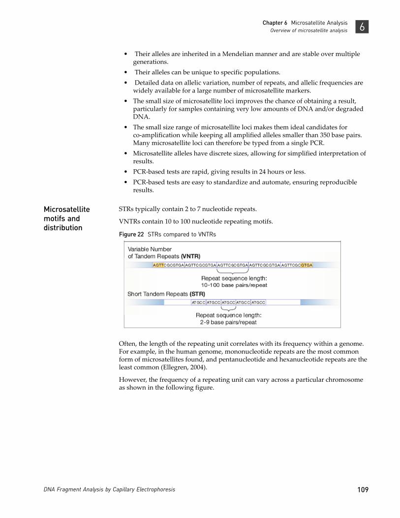
109DNA Fragment Analysis by Capillary Electrophoresis
Chapter 6 Microsatellite AnalysisOverview of microsatellite analysis 6
• Their alleles are inherited in a Mendelian manner and are stable over multiple generations.
• Their alleles can be unique to specific populations. • Detailed data on allelic variation, number of repeats, and allelic frequencies are
widely available for a large number of microsatellite markers. • The small size of microsatellite loci improves the chance of obtaining a result,
particularly for samples containing very low amounts of DNA and/or degraded DNA.
• The small size range of microsatellite loci makes them ideal candidates for co‐amplification while keeping all amplified alleles smaller than 350 base pairs. Many microsatellite loci can therefore be typed from a single PCR.
• Microsatellite alleles have discrete sizes, allowing for simplified interpretation of results.
• PCR‐based tests are rapid, giving results in 24 hours or less.• PCR‐based tests are easy to standardize and automate, ensuring reproducible
results.
Microsatellite motifs and distribution
STRs typically contain 2 to 7 nucleotide repeats.
VNTRs contain 10 to 100 nucleotide repeating motifs.
Figure 22 STRs compared to VNTRs
Often, the length of the repeating unit correlates with its frequency within a genome. For example, in the human genome, mononucleotide repeats are the most common form of microsatellites found, and pentanucleotide and hexanucleotide repeats are the least common (Ellegren, 2004).
However, the frequency of a repeating unit can vary across a particular chromosome as shown in the following figure.

110 DNA Fragment Analysis by Capillary Electrophoresis
Chapter 6 Microsatellite AnalysisApplications6
Figure 23 SSR density in exonic, intronic and intergenic regions on individual human chromosomes: (a) monomers (b) dimers; (c) trimers; (d) tetramers; (e) pentamers; (f) hexamers. Blue bars, exons; red bars, introns; yellow bars, intergenic regions (http://www.ncbi.nlm.nih.gov/pmc/articles/PMC151303/figure/F2/ Copyright 2003, Subramanian et al.; licensee BioMed Central Ltd. This is an Open Access article: verbatim copying and redistribution of this article are permitted in all media for any purpose, provided this notice is preserved along with the article's original URL.)
Applications
The large selection of highly informative markers has made microsatellite analysis a widely accepted tool for the following types of studies:
• Linkage mapping studies• Association studies• Population studies• Parentage analysis• Breeding
Custom microsatellite assays are often used for:
• Cancer progression analysis• Phylogenetic studies• Genome scans for an organism where commercial marker panels are not available• Population genetics studies• Paternity testing• Parentage analysis for selective breeding
111DNA Fragment Analysis by Capillary Electrophoresis
Chapter 6 Microsatellite AnalysisInstrument and consumable recommendations 6
Instrument and consumable recommendations
This is a “Thermo Fisher Scientific‐supported” protocol.
• Thermal cycler: 2720, Veriti®, or GeneAmp® 9700• Genetic analyzer: 3500 Series, 3130 Series, or 310 instrument• Polymer and capillary array: see “Run modules” on page 69 for the polymer and
capillary array length combinations supported on each instrument• 600 LIZ® Size Standard• DS‐33 G5 dye set• AmpliTaq® and AmpliTaq Gold® DNA Polymerases are typically used for
microsatellite analysis. Like other DNA polymerases, these polymerases may catalyze the addition of a single nucleotide (usually A, adenosine) to the 3’ ends of the two strands of a double‐stranded DNA fragment. For more information, see “Addition of 3ʹ A nucleotide by Taq polymerase” on page 33 and Witmer et al., 2003.
IMPORTANT! Throughout a set of experiments, use the same equipment, run parameters, polymers, dyes, and so on. Consistent conditions are required to avoid mobility shifts that interfere with accurate interpretation of data.
Experiment and primer design recommendations
• Identify the markers for your study by examining the existing scientific literature for a specific marker or cross‐species marker, or by following a microsatellite development protocol (Fleischer and Lowe, 1995; Kandpal et. al., 1994).
• The discovery and random naming of new microsatellite markers across different organisms at multiple institutions has led to inconsistent nomenclatures for microsatellites. For more information on nomenclature standards for specific genomes, go to the nomenclature website of the institution, a few of which are listed below.– Human: https://iris.ucl.ac.uk– Rat/mouse: http://rgd.mcw.edu/– Fly: http://flybase.org/
• Design primers so the range of amplicon lengths across markers in the study spans is within the size‐standard fragment range, with two size‐standard peaks preceding the smallest fragment of interest and two size‐standard peaks following the largest fragment of interest.
• Use 5´‐end labeled primers. The success of microsatellite analysis depends upon the ability to detect small mobility differences. The reproducible sizing and sharp peaks obtained when using the 5´‐end labeling method are crucial to the success of this application.
• If you plan to multiplex, design primers with similar annealing temperatures ~60°C.
• Use reverse‐primer tailing on one primer in each set of primers to help differentiate between peaks made by the forward and reverse DNA strands and to promote A addition. See “Tail” on page 34 for more information.

112 DNA Fragment Analysis by Capillary Electrophoresis
Chapter 6 Microsatellite AnalysisWorkflow 6
• Based on sample DNA concentration, robustness of the PCR, and/or peak heights observed in capillary electrophoresis, determine whether you need to dilute the PCR products. Dilutions can range from undiluted to 1:20 in water. You can pool the diluted PCR products if desired.
• Dye‐labeled PCR products must be mixed in different ratios because each dye has a slightly different fluorescence signal strength (see “Emission and absorption (excitation) wavelengths and relative intensities” on page 38).
• To avoid inaccuracies associated with pipetting small volumes, prepare a master mix of reagents. Prepare sufficient master mix for at least one extra reaction volume.
• Store the master mix in the dark at 2 to 6°C for up to 1 month, or at –15 to –25°C for longer.
• A typical reaction may include: 1 μL of each PCR product and 0.5 μL of the GeneScan™ size standard in 8.5 μL of Hi‐Di™ formamide (for denaturing applications) or distilled, deionized water (for non‐denaturing applications).
• Master‐mix reagents are optimized for capillary electrophoresis, and differ depending on the capillary electrophoresis instrument you use.
Workflow
1. Select primers and size standards:
a. Design and order primers for a microsatellite application.
b. Optimize amplification conditions with microsatellite markers on test DNA.
c. Order dye‐labeled primers.
2. PCR
3. Capillary electrophoresis
4. Data analysis
Data analysis
The GeneMapper® Software includes a Microsatellite Default analysis method that you can use as a starting point for analysis.
Figure 24 on page 113 shows a typical microsatellite electropherogram from the GeneMapper® Software.
The number of repeats for a given locus may vary, resulting in alleles of differing lengths. The following figure shows two different FAM™dye‐labeled human dinucleotide loci (from the GeneMapper® Software tutorial dataset) from two individuals. The top panel illustrates a DNA sample that is homozygous at both loci (a single major peak is observed at each locus), the bottom panel shows a DNA sample that is heterozygous at the same loci (two major peaks are observed at each locus).

113DNA Fragment Analysis by Capillary Electrophoresis
Chapter 6 Microsatellite AnalysisCommon problems with microsatellite analysis 6
Figure 24 Example of microsatellite analysis of two samples by capillary electrophoresis. Samples have different genotypes as shown by the different peaks for the same marker.
Common problems with microsatellite analysis
The most commonly encountered problems during microsatellite analysis are:
• Poor or non‐specific amplification. See “Optimizing PCR” on page 55 and “PCR troubleshooting” on page 176.
• Incomplete 3´ A nucleotide addition. See “Incomplete 3ʹ A nucleotide addition” on page 33.
• Stutter. See the next section.
See Chapter 11, “Troubleshooting” on page 151 for more information on stutter peaks and plus A products.
Identifying stutter products in microsatellite analysis
Overview During the PCR amplification of di‐, tri‐, and tetranucleotide microsatellite loci, minor products that are 1 to 4 repeat units shorter than the main allele are produced. The minor product peaks are referred to as “stutter” peaks. Stutter peaks may be caused by polymerase slippage during elongation (Hauge and Litt, 2003; Murray and Lai, 2003).

114 DNA Fragment Analysis by Capillary Electrophoresis
Chapter 6 Microsatellite AnalysisIdentifying stutter products in microsatellite analysis6
Stutter peaks appear as multiple lower peaks that precede the true allele peak. These stutter peaks differ in size from the true allele peak by multiples of the length of the repeat unit. The number of peaks and their intensities are proportional to the length of the repeat and the number of repeats in the PCR product (Shinde et. al. 1993). Shorter repeat units (di‐ or tri‐, for ex.) generate more stutter, and dinucleotide repeats tend to generate more stutter peaks than trinucleotide repeats.
Stutter peaks can also be caused by off‐scale data. For more information, see “Evaluating data with stutter” on page 117.
GeneMapper® Software is optimized to filter out stutter peaks.
Estimating the amount of stutter
You can estimate the percent stutter by calculating the ratio of the combined heights of the stutter peaks with the height of the true allele peak. Note the following:
• The longer the repeat unit, the less stutter product produced. For microsatellite loci with the same number of repeat units, the percent stutter is greater for dinucleotide microsatellite loci than it is for trinucleotide microsatellite loci, and so on (Walsh et al., 1996).The figure below illustrates the greater stutter in dinucleotide (left) as compared to tetranucleotide (right) repeat loci. Each locus is homozygous, with the largest peak in each figure representing the “true” allele.
• The percent stutter increases with increasing allele length (that is, with increasing number of repeat units). However, if some of the repeats are partial repeats, you may not see the proportionate increase in percent stutter.

115DNA Fragment Analysis by Capillary Electrophoresis
Chapter 6 Microsatellite AnalysisIdentifying stutter products in microsatellite analysis 6
Figure 25 Stutter percentages for the FGA and TH01 loci. (Black data points indicate loci labeled with NED™ dye.)
Dinucleotide repeats
Successful amplification of dinucleotide repeat markers yields allele peaks and associated stutter peaks within a maximum range of eight base pairs from the allele peak. In addition, the number of allele peaks depends on whether the individual tested is a heterozygote or homozygote.
Dinucleotide repeats in a homozygous individual
The GeneMapper® Software electropherogram of a dinucleotide repeat marker from a homozygous individual (190 bp, 190 bp) is shown in the following figure.
Figure 26 Stutter peaks in a dinucleotide repeat electropherogram (homozygote)

116 DNA Fragment Analysis by Capillary Electrophoresis
Chapter 6 Microsatellite AnalysisIdentifying stutter products in microsatellite analysis6
The peaks at 188 bp, 186 bp, and 184 bp show the typical 2‐bp stutter pattern seen with dinucleotide repeats. They represent the –2 bp, –4 bp, and –6 bp stutter peaks from the true 190‐bp true allele peak.
Dinucleotide repeats in a heterozygous individual (8 bp)
The GeneMapper® Software electropherogram of a dinucleotide repeat marker from a heterozygous individual (139 bp, 147 bp) is shown in the following figure. Allele sizes differ by 8 bp.
The 2‐bp stutter peak to the left of each allele peak is always of lower intensity than the allele peak itself. The larger 147‐bp allele peak is of lower intensity than the smaller 139‐bp allele. In heterozygotes, the higher molecular weight allele (that is, the allele peak further to the right in electropherograms) often produces a fluorescence signal of lower intensity than the lower molecular weight allele, suggesting a less efficient amplification of the larger fragment. This phenomenon could also be caused by preferential injection of the smaller fragments.
Figure 27 Stutter peaks in a dinucleotide repeat electropherogram (heterozygote 8 bp)
Dinucleotide repeats in a heterozygous individual (4 bp)
The GeneMapper® Software electropherogram from a dinucleotide repeat marker of a heterozygous individual (185 bp, 189 bp) is shown in the following figure. Allele sizes differ by 4 bp.
Figure 28 Stutter peaks in a dinucleotide repeat electropherogram (heterozygote 4 bp)

117DNA Fragment Analysis by Capillary Electrophoresis
Chapter 6 Microsatellite AnalysisIdentifying stutter products in microsatellite analysis 6
When the difference between the allele sizes is ≤4 bp, a shift occurs in the height ratio between the two allele peaks (compare the two preceding figures). The fluorescence signal from the –4 bp stutter of the 189‐bp allele is added to the signal from the 185‐bp allele.
Dinucleotide repeats in a heterozygous individual (2 bp)
The GeneMapper® Software electropherogram from a dinucleotide repeat marker of a heterozygous individual (216 bp, 218 bp) is shown in the following figure. Allele sizes differ by 2 bp.
Figure 29 Stutter peaks in a dinucleotide repeat electropherogram (heterozygote 2bp)
When the difference between the allele sizes is ≤2 bp, the fluorescence signal from the –2 bp stutter of the larger base pair allele does not appear as a separate stutter peak. It is added to the signal of the smaller base pair allele.
Evaluating data with stutter
The multipeak pattern seen with stutter peaks can complicate analysis, particularly for samples with two or more alleles that are close in size. For example, small peaks in a position that is one repeat unit smaller than the true allele can be interpreted either as a stutter peak or as an allele in a minor component of a mixed sample. The possible presence of stutter peaks makes precise quantitation especially important, to allow the GeneMapper® Software filtering algorithm to interpret the peak pattern accurately.
The percent stutter for a given allele is reproducible and does not depend on the quantity of input DNA or the number of loci amplified during multiplex PCR. The relative reproducibility of percent stutter is important for a few reasons:
• In many cases, you can adjust the Peak Amplitude Threshold in the analysis method of the GeneMapper® Software to filter out stutter peaks and detect only true allele peaks. Fore more information, refer to the GeneMapper® Software Getting Started Guide: Microsatellite Analysis (Pub. no. 4403672).
• Amplifications with an abnormally high percent stutter can indicate mixed samples or some other problem with PCR amplification or electrophoresis.
Stutter band
Stutter from 218 bp peak is added to the 216 bp peak

118 DNA Fragment Analysis by Capillary Electrophoresis
Chapter 6 Microsatellite AnalysisFor more information6
Is stutter a real problem?
Stutter, once understood, does not pose a real problem for microsatellite analysis and can aid in allele calling by:
• Distinguishing true allele peaks from non‐specific PCR products. Non‐specific PCR products are not associated with stutter peaks.
• Identifying alleles that fall far outside the reported allele range. The percent stutter is often specific to a particular locus. You can sometimes identify alleles that fall far outside the previously reported range on the basis of percent stutter.
For more information
See “Microsatellite applications” on page 200.

119DNA Fragment Analysis by Capillary Electrophoresis
7 Single Nucleotide Polymorphism(SNP) Genotyping
■ Overview of SNP genotyping. . . . . . . . . . . . . . . . . . . . . . . . . . . . . . . . . . . . . . . . . . 119
■ SNaPshot® Multiplex System. . . . . . . . . . . . . . . . . . . . . . . . . . . . . . . . . . . . . . . . . . 120
Overview of SNP genotyping
Overview A Single Nucleotide Polymorphism (SNP) marker consists of a single base pair that varies in the known DNA sequence, thereby creating up to four alleles or variations of the marker.
SNP markers occur in the human genome at a frequency of about 1 in every 1000 bp, with a total number of over 10 million SNP markers distributed evenly over the 3 billion bps of the human genome. They have been shown to be responsible for differences in genetic traits, susceptibility to disease, and response to drug therapies. SNP markers are excellent genetic markers to construct high‐resolution genetic maps.
SNP markers can be genotyped by a variety of methods. Thermo Fisher Scientific products support the following methods:
• Single‐base extension• Shifted Termination Assay (STA) primer extension
Applications (SNP) Some applications of SNP genotyping include:
• Study of mutations implicated in various cancers• Genetic disease research• Mitochondrial DNA investigations• Scrapie susceptibility in sheep• Loss of heterozygosity• Assess performance in food animal production, • Differentiate drug and non‐drug forms of Cannabis
...TCGTTGTAGCGCTTAGA......AGCAACATCGCTAATCT...
...TCGTTGTAACGCTTAGA......AGCAACATTGCTAATCT...
The G-C and A-T base pairs are two possible alleles of this SNP site

120 DNA Fragment Analysis by Capillary Electrophoresis
Chapter 7 Single Nucleotide Polymorphism (SNP) GenotypingSNaPshot® Multiplex System7
SNaPshot® Multiplex System
Components The SNaPshot® Multiplex System investigates up to ten SNP markers simultaneously by using PCR amplification, then dideoxy single‐base extension of an unlabeled primer, and then capillary electrophoresis. After electrophoresis and fluorescence detection, the alleles of a single marker appear as different colored peaks at roughly the same size in the electropherogram plot. The size of the different allele peaks will vary slightly due to differences in molecular weight of the dyes.
Figure 30 Overview of the SNaPshot® kit assay
Components of the system are:
• SNaPshot® Multiplex Kit – Includes SNaPshot® Multiplex Ready Reaction Mix, control primer mix, and control template.
• SNaPshot® Primer Focus® Kit – Designed to determine the approximate fragment sizes generated by various primers before SNP genotyping (critical if two oligonucleotides produce overlapping signals when run simultaneously) and enables the setting of tight loci‐windows in GeneMapper® Software.
• GeneScan™ 120 LIZ® Size Standard – Five‐dye size standard that is designed for reproducible sizing of small fragment analysis data generated with the SNaPshot® Multiplex Systems. It accurately sizes samples ranging from 20 to 120 nucleotides (nt). When used with GeneMapper® Software, the GeneScan™ 120 LIZ® Size Standard eliminates the need for manual genotyping.
• Matrix Standard Set DS‐02 – Used for spectral calibration.• GeneMapper® Software – Genotype analysis for data generated with SNaPshot®
Multiplex Systems.

121DNA Fragment Analysis by Capillary Electrophoresis
Chapter 7 Single Nucleotide Polymorphism (SNP) GenotypingSNaPshot® Multiplex System 7
Additionally, the SNaPshot® Primer Focus® Kit allows rapid assessment of potential SNP oligonucleotides. You can preview all potential single‐base extension products and calculate the mobility rate for each allele. After assessing this data, you can determine the optimal combination of SNP markers for multiplexing. After you determine the multiplex format, you can use the reference data created with the Primer Focus Kit to establish markers and bin sets in the GeneMapper® Software, and reduce the time required to define and edit bins manually.
Principle of the analysis
In the single‐base extension technique, a unlabeled primer is designed to anneal to the sequence adjacent to the SNP site. After the primer anneals, the single‐base extension occurs by the addition of the complementary dye‐labeled ddNTP (dye terminator) to the annealed primer. Each of the four ddNTPs is fluorescently labeled with a different color dye (Figure 31).
Figure 31 Single-base extension with dye-labeled ddNTPs
The addition of ddNTPs yields marker fragments for the different SNP alleles that are all the same length, but vary by color.
After electrophoresis and fluorescence detection, the alleles of a single marker appear as different colored peaks at roughly the same size in the electropherogram plot. The size of the different allele peaks will vary slightly due to differences in molecular weight of the dyes.
Advantages • Uses unlabeled user‐defined primers that are customized for your target• Offers multiplexing capability (up to 10‐plex, regardless of their positions on the
chromosome or the amount of separation from neighboring SNP loci)• Sensitive allele frequency detection (5%)• Compatible with all Thermo Fisher Scientific genetic analyzers• Automated analysis using specific GeneMapper® Software data analysis module
Additionally, the SNaPshot® kit can be used for a variety of other applications:
• BAC fingerprinting• DNA methylation
Applications (SNaPshot®)
• Low‐to‐medium throughput linkage and association studies • Single‐locus fragment analysis
Template DNA
Unlabeled primerDye-labeled ddNTPs

122 DNA Fragment Analysis by Capillary Electrophoresis
Chapter 7 Single Nucleotide Polymorphism (SNP) GenotypingSNaPshot® Multiplex System7
• Screen and confirm SNPs• Screen for prion gene mutation
Screen and confirm SNPs
The SNaPshot® Multiplex System includes a variety of SNaPshot® Multiplex Kits used for SNP screening and validation. Each kit offers a one‐tube single‐base extension/termination reagent to label DNA fragments.
Screen for Prion gene mutations
The single base‐pair sensitivity of the SNaPshot® Multiplex System enables you to accurately screen samples for codon differences in prion genes. Prion diseases are caused by abnormally folded isoforms of host‐encoded proteins. Use the SNaPshot® Multiplex System to screen for SNPs in the genes that code for these proteins. For instance, polymorphisms at codons 136, 154 and 171 of the PrP gene in sheep and goats can lead to abnormally folded isoforms of the protein product to result in scrapie.
Instrument and consumable recommendations
• Thermal cycler: Veriti®, or GeneAmp® 9700 (for fast thermal cyclers, use a 1°C/second ramp rate), 2720
• Genetic analyzer: 3500 Series, 3730 Series, 3130 Series, or 310 instruments• Polymer and capillary array: see “Run modules” on page 69 for the polymer and
capillary array length combinations supported on each instrument• GeneScan™ 120 LIZ® Size Standard• DS‐02 dye set
IMPORTANT! Throughout a set of experiments, use all the same equipment, run parameters, polymers, dyes, and so on. Consistent conditions are required to avoid mobility shifts that interfere with accurate interpretation of data.

123DNA Fragment Analysis by Capillary Electrophoresis
Chapter 7 Single Nucleotide Polymorphism (SNP) GenotypingSNaPshot® Multiplex System 7
Experiment and primer design recommendations
This is a “Thermo Fisher Scientific‐supported” protocol.
• Minimum primer length is 23 nt, however it is strongly recommended that primers shorter than 36 nt be tested before multiplexing.
• HPLC purification of primers longer than 30 nt is recommended. Heterogeneous primer populations will lead to major analysis issues.
• Each primer should have 23 nt complimentary to the gDNA sequence. • Use 5’ tails to create different length primers.• Add poly (dGACT) to generate a size difference of at least 4 to 6 nt.• Primers can be complimentary to the (‐) strand of the DNA if the (+) strand is
difficult to assay.• Always run a negative control (no template DNA) when evaluating a new primer.
Workflow 1. Design primers.
2. Prepare template by PCR of target, then clean‐up
3. Prepare SNaPshot® reactions
4. Post‐extension by PCR, then clean‐up
5. Capillary electrophoresis
6. Analyze data
Data analysis The GeneMapper® Software includes a SNaPshot® Default analysis method that you can use as a starting point for analysis.
For more information
For documents and publications, see “SNP applications” on page 201.
An extensive list of publications demonstrating the utility of the SNaPshot® Multiplex System is available at www.lifetechnologies.com.
For ordering information, see “SNaPshot® Kits” on page 198.

124 DNA Fragment Analysis by Capillary Electrophoresis
Chapter 7 Single Nucleotide Polymorphism (SNP) GenotypingSNaPshot® Multiplex System7

125DNA Fragment Analysis by Capillary Electrophoresis
8 Fingerprinting
■ Overview . . . . . . . . . . . . . . . . . . . . . . . . . . . . . . . . . . . . . . . . . . . . . . . . . . . . . . . . . . . 125
■ Amplified fragment length polymorphism (AFLP®) Analysis. . . . . . . . . . . . . . 126
■ Terminal restriction fragment length polymorphism (T‐RFLP) . . . . . . . . . . . . . 131
■ Bacterial Artificial Chromosome (BAC) fingerprinting . . . . . . . . . . . . . . . . . . . . 132
■ High coverage expression profiling (HiCEP). . . . . . . . . . . . . . . . . . . . . . . . . . . . . 136
■ Inter‐simple sequence repeat (ISSR) PCR . . . . . . . . . . . . . . . . . . . . . . . . . . . . . . . . 137
Overview
DNA fingerprinting is a technique that is used to identify patterns that occur in genetic markers. These fingerprints are specific to particular organisms. A number of techniques are available for fingerprinting.

126 DNA Fragment Analysis by Capillary Electrophoresis
Chapter 8 FingerprintingAmplified fragment length polymorphism (AFLP®) Analysis8
Amplified fragment length polymorphism (AFLP®) Analysis
Amplified fragment length polymorphism (AFLP®) is a mapping technique used to visualize polymorphisms in genomic DNA. The AFLP® system combines the restriction fragment length polymorphism (RFLP) technique and polymerase chain reaction (PCR) to generate a large number of amplified restriction fragments from prepared, genomic DNA. When separated by electrophoresis, the samples yield unique band patterns that, when visualized by southern blot or fluorescence‐based fragment analysis, can be used for high‐resolution genotyping, polymorphism detection, or cladistics (Savelkoul et al. 1999).
Principle of the analysis
The AFLP® procedure involves digesting genomic DNA to produce a population of restriction fragments, ligation of priming sites, then amplified by PCR. (Goel et al. 2006.) It is sometimes considered a variation of random amplified polymorphic DNA (RAPD).
Figure 32 AFLP® analysis
AFLP® is possible because the abundant complexity in eukaryotic genomic DNA means that it is statistically likely that enough restriction fragments will be short enough to successfully produce PCR amplicons that yield a unique “fingerprint” profile.
Advantages The power of AFLP® analysis derives from its ability to quickly generate large numbers of marker fragments for any organism, without prior knowledge of the genomic sequence. In addition, AFLP® analysis requires only small amounts of starting template and can be used for a variety of genomic DNA samples.
Restriction digestion
Ligation
Preselective amplification
Selective amplification
ElectrophoresisSample 1
Sample 2
Sample 3
127DNA Fragment Analysis by Capillary Electrophoresis
Chapter 8 FingerprintingAmplified fragment length polymorphism (AFLP®) Analysis 8
Applications Fingerprints, or AFLP® band patterns, can be used for many purposes. For example, AFLP® analysis is often used in plant research where fingerprints can be compared to determine the plant variety or to compare the similarities between different plant varieties.
Thermo Fisher Scientific provides kits for performing AFLP® on microbes and plants, and reagents that are useful for performing AFLP® on other organisms. Some additional applications for AFLP® analysis include:
• Molecular diversity studies (Zhao et al. 2006 and Johnson et al. 2005.)• Phylogeny studies (Goel et al. 2006.)• Breeding (Zhao et. al., ibid.)• Backcross studies (Johnson et al. and Goel et al., ibid.) • Mapping of cloned fragments in bacterial and yeast artificial chromosomes (BACs
and YACs) (Serra, et al. 2006, Naimuddin, et al. 2004)• Identifying new species or subspecies (Johnson et al. ibid., and Savelkoul, et al.
1999.)
The AFLP® kits available from Thermo Fisher Scientific are optimized for plants and microbes. However, they are an excellent starting point for custom AFLP experiments on other organisms (such as fish). Contact your Thermo Fisher Scientific field applications specialist for more information on using Applied Biosystems®AFLP kits to conduct experiments in organisms other than plants or microbes.
Instrument and consumable recommendations
This is a “Thermo Fisher Scientific‐supported” protocol.
• Thermal cycler: Veriti® (standard mode only), GeneAmp® 9700, 2720• Genetic analyzer: 3500 Series, 3730 Series, 3130 Series, or 310 instruments• Polymer: see “Run modules” on page 69 for the polymer and capillary array
length combinations supported on each instrument• Capillary array:
– 3500 Series instruments: 50‐cm– 3730 Series, 3130 Series, and 310 instruments: 36‐cm
• GeneScan™ 500 ROX™ Size Standard (included in kits)• DS‐32 Matrix Standard (Dye Set F)
IMPORTANT! Throughout a set of experiments, use all the same equipment, run parameters, polymers, dyes, and so on. Consistent conditions are required to avoid mobility shifts that interfere with accurate interpretation of data.
Experiment and primer design recommendations
DNA extraction and purification
Because AFLP® analysis requires only a small amount of DNA (50 to 500 ng, ideally 10 to 100 ng), DNA purification is critical.
We recommend the following kits for extracting DNA for AFLP analysis:
• Plant Analysis: DNAzol® Reagent or PureLink® Genomic Plant DNA Purification Kit
• Microbial Analysis: PureLink® Genomic DNA Mini Kit

128 DNA Fragment Analysis by Capillary Electrophoresis
Chapter 8 FingerprintingAmplified fragment length polymorphism (AFLP®) Analysis8
Restriction
In AFLP® experiments on genomes of unknown content, determine whether or not your genomic DNA restricts properly with EcoRI and MseI enzymes.
In general, the Regular Plant Genome Kit modules should produce quality genetic fingerprints with genomes of 5x10⁸ to 6✕109 base pairs, and the Small Plant Genome Kit modules with genomes of 5x10⁷ to 5✕108 base pairs.
Empirical guidelines suggest that if the G+C content of the genome is >65%, MseI will not give a significant number of fragments. Optimal results are obtained with MseI when the G+C content is <50%. EcoRI also tends to produce more fragments in G+C‐ poor genomes. In cases where an organismʹs G+C content is unknown, the effectiveness of the restriction enzymes must be determined empirically.
Primers
For the selective amplification step, the primers that target the EcoRI/A binding site are fluorescently labeled at the 5ʹ end. The primers that target the MseI/C binding site are unlabeled.
You may need to optimize to identify primer combinations that generate sufficient unique marker fragments for a study.
For example, the Plant Mapping Kits contain eight selective forward primers and eight reverse primers labeled with the 5‐FAM™, NED™, and JOE™ dye‐labeled fluorophores (Dye Set F). The possible combinations of forward and reverse primers provides 128 possible primer combinations that have been tested across several crop genomes, facilitating identification of the optimal pair(s) for a given organism without having to design, synthesize, or perform quality control tests of custom primers.
The Appendix of the AFLP® Plant Mapping Protocol (Pub. no. 4303146) shows primer combinations that have been successfully used for a variety of plant species and the AFLP® Microbial Fingerprinting Protocol (Pub. no. 402977) shows primer combinations that have been successfully used for a variety of microbial organisms. (Note that if your organism of interest does not appear in the list, you can still conduct experiments by choosing primers from the most closely related species that is available.)
In general, the strategy with AFLP® analysis is to generate informative fragments, or enough fragments so that individuals are distinguishable. However, too many fragments complicate the analysis, so you must empirically determine the optimum number of fragments needed for adequate discrimination. As a general rule, it is best to have between 50 and 200 peaks as the “fingerprint” after amplification.
Workflow 1. Restriction digestion
2. Ligation
3. Preselective amplification
4. Selective amplification
5. Capillary electrophoresis
6. Data analysis

129DNA Fragment Analysis by Capillary Electrophoresis
Chapter 8 FingerprintingAmplified fragment length polymorphism (AFLP®) Analysis 8
Data analysis The GeneMapper® Software includes an AFLP® Default analysis method that you can use as a starting point for analysis.
This method contains analysis parameters for pattern recognition of fragments across samples to generate a fingerprint for every sample. This method can be used to analyze any type of data from fragment length polymorphism assays such as AFLP or T‐RFLP. Features of the software useful for analysis include:
• Ability to generate a panel (the collection of markers) from sample files that have been added to a project.
• Sizing Quality and Genotyping Quality values flag poor quality samples enabling easy identification and decrease manual review.
• Automatic generation of final marker genotypes in a standard binary format where “1” represents the presence of a given fragment while “0” represents the absence of the corresponding fragment.
Up to four profiles are expected for each sample because:
• Both the forward and reverse PCR primers may be fluorescently labeled• Two restriction enzymes are used
Generate panels and binsets using the AFLP Default analysis method. You can then routinely analyze data using this panel.
A change in the fragment profile can be indicated by the absence of a peak as well as a reduction in the height of a peak when comparing different samples.
The following two figures are examples of typical and polymorphic AFLP® reactions.
Figure 33 Typical electropherogram of an AFLP reaction

130 DNA Fragment Analysis by Capillary Electrophoresis
Chapter 8 FingerprintingAmplified fragment length polymorphism (AFLP®) Analysis8
Figure 34 Polymorphic AFLP peaks
These peak patterns are automatically converted to a table of binary marker genotypes (Figure 35), which can be exported and analyzed for similarity and generation of dendrograms using a statistical software package or other downstream analysis software for this type of clustering analysis.
Figure 35 AFLP genotypes in GeneMapper® Software
For more information
For documents and publications, see “AFLP® applications” on page 200.
For ordering information, see “Ordering Information” on page 193.

131DNA Fragment Analysis by Capillary Electrophoresis
Chapter 8 FingerprintingTerminal restriction fragment length polymorphism (T-RFLP) 8
Terminal restriction fragment length polymorphism (T-RFLP)
Overview Terminal restriction fragment length polymorphism (T‐RFLP) analysis is a mapping technique used to study complex microbial communities based on variation in the 16S rRNA gene (Osborn and Moore et.al.). It is culture‐independent, rapid, sensitive, and reproducible and does not require genomic sequence information.
Principle of the analysis
In T‐RFLP analysis, fluorescently labeled DNA is digested with restriction enzymes that have 4 base‐pair recognition sites. This step generates fluorescently labeled terminal restriction fragments. The fragments in the digest are then separated by capillary electrophoresis. Profiles can then be compared between samples, or matched to a database of known species.
Applications • Examine microbial community structure and community dynamics in response to changes in different environmental parameters or to study bacterial populations in natural habitats.
• Study of complex microbial communities in diverse environments such as soil (Derakshani and Lukow et.al.), marine and activated sludge systems (Eschenhagen and Schuppler et al.)
• Characterize oral bacterial flora in saliva in healthy subjects versus patients with periodontitis (Sakamoto and Takeuchi et al.).
• Preliminary screening of microorganisms before analysis using Applied Biosystems® MicroSEQ® Microbial identification kits.
Instrument and consumable recommendations
This is a “Thermo Fisher Scientific‐demonstrated” protocol.
• Thermal cycler: Veriti®, GeneAmp® 9700, 2720• Genetic analyzer: 3500 Series, 3730 Series, 3130 Series, and 310 instruments• Polymer: see “Run modules” on page 69 for the polymer and capillary array
length combinations supported on each instrument• GeneScan™ 600 LIZ® Size Standard• DS‐33 Matrix Standard (Dye Set G)
IMPORTANT! Throughout a set of experiments, use all the same equipment, run parameters, polymers, dyes, and so on. Consistent conditions are required to avoid mobility shifts that interfere with accurate interpretation of data.

132 DNA Fragment Analysis by Capillary Electrophoresis
Chapter 8 FingerprintingBacterial Artificial Chromosome (BAC) fingerprinting8
Experiment and primer design recommendations
Follow the recommendations for AFLP® analysis. See “Experiment and primer design recommendations” on page 127.
Workflow
1. DNA isolation and purification.
2. PCR amplification and restriction enzyme digestion.
3. Separation and detection of the digested products via electrophoresis.
4. Analysis of data to generate the fragment profile for each sample.
5. Clustering analysis based on the profile of samples from step 4.
Data analysis T‐RFLP analysis uses the same data analysis technique as AFLP. See “Data analysis” on page 129.
For more information
For documents and publications, see “AFLP® applications” on page 200.
For ordering information, see “Ordering Information” on page 193.
Bacterial Artificial Chromosome (BAC) fingerprinting
Overview BAC fingerprinting provides an efficient and cost‐effective method of characterizing large genomic fragment libraries for genome sequencing, positional cloning, and physical mapping efforts. Restriction endonuclease digestion of BAC clones followed by fluorescent‐dye labeling can be used to generate a profile or fingerprint. Overlap between fingerprints are subsequently used to assemble contiguous sequences (contigs) in the construction of whole‐genome physical maps. Physical maps are important resources for genome sequencing efforts, positional cloning, comparative genomics, and to determine the size and structure of genomes.
The SNaPshot® Multiplex Kit (Luo et al.) provides an effective, easy, and cost‐effective solution for high‐throughput BAC fingerprinting.
DNA extraction
PCR with labeled primers
Digestion with restriction enzymes
ElectrophoresisData analysis

133DNA Fragment Analysis by Capillary Electrophoresis
Chapter 8 FingerprintingBacterial Artificial Chromosome (BAC) fingerprinting 8
Principle of the analysis
In BAC fingerprinting analysis using the SNaPshot® Multiplex Kit, BAC clones are subjected to restriction‐endonuclease to generate fragments of various lengths that end in A, C, G, or T. The SNaPshot® chemistry then labels the fragments with the corresponding bases by single‐base extension to create a distinct DNA fragment pattern or “fingerprint” for each clone. The clones are then mapped based on the order of the overlapping parts of “fingerprints” with other clones of the same genome.
Figure 36 SNaPshot restriction fragment labeling
Table 19 Example of possible six-base cutters for restriction endonucleases and dyes used in the SNaPshot® Multiplex Kit
Applications With BAC fingerprinting, you can create whole‐genome physical maps that are important resources for:
• Genome sequencing• Positional cloning• Comparative genomics
Restriction endonuclease
Restriction site ddNTP Fluorescent
dyeRestriction fragment
color
EcoRI G¯AATTC A dR6G Green
BamHI G¯GATCC G dR110 Blue
XbaI T¯CTAGA C dTAMRA™ Yellow
XhoI C¯TCGAG T dROX™ Red
HaeIII GG¯CC None — —
Recessed strand
Label template
SNaPshot reaction mix
Color = genotypeElectrophoresis

134 DNA Fragment Analysis by Capillary Electrophoresis
Chapter 8 FingerprintingBacterial Artificial Chromosome (BAC) fingerprinting8
Instrument and consumable recommendations
This is a “Thermo Fisher Scientific‐demonstrated” protocol.
IMPORTANT! BAC fingerprinting is based upon pattern recognition; therefore, data analysis is focused on relative size and distribution. We recommend using a dedicated instrument platform to minimize low random error caused by sizing imprecision.
• Thermal cycler: Veriti®, GeneAmp® 9700, 2720• Genetic analyzer: 3500 Series, 3730 Series, 3130 Series, and 310 instruments• Polymer: see “Run modules” on page 69 for the polymer and capillary array
length combinations supported on each instrument• Capillary array:
– 3500 Series instruments: 50‐cm– 3730 Series, 3130 Series, and 310 instruments: 36‐cm
• GeneScan™ 120 LIZ® Size Standard• DS‐33 Matrix Standard (Dye Set G5)
IMPORTANT! Throughout a set of experiments, use all the same equipment, run parameters, polymers, dyes, and so on. Consistent conditions are required to avoid mobility shifts that interfere with accurate interpretation of data.
Experiment and primer design recommendations
• Protocols may differ based on the kind of restriction endonucleases and the BAC DNA purification kits that are used.
• Enzymatic digestion and SNaPshot® reagent labeling can be performed in one tube or in separate reactions.

135DNA Fragment Analysis by Capillary Electrophoresis
Chapter 8 FingerprintingBacterial Artificial Chromosome (BAC) fingerprinting 8
Workflow
1. Selective bacterial growth of single colonies.
2. BAC purification by restriction‐endonuclease digestion.
3. Restriction‐endonuclease digestion of the BAC clones with several different enzymes.
4. SNaPshot®‐reagent labeling of fragments. The dye‐labeled primers are bound to the BAC fragments based on the overhangs left by the restriction enzymes (see Table 19 on page 133).
5. Post‐extension clean‐up of the clones (not shown in diagram).
6. Capillary electrophoresis.
7. Data analysis.
8. Contig construction.
Data analysis See “BAC applications” on page 200.

136 DNA Fragment Analysis by Capillary Electrophoresis
Chapter 8 FingerprintingHigh coverage expression profiling (HiCEP)8
For more information
For documents and publications, see “BAC applications” on page 200.
For ordering information, see “Ordering Information” on page 193.
High coverage expression profiling (HiCEP)
Overview The high coverage expression profiling (HiCEP) method of fragment analysis was developed to address the shortcomings in gene expression profiling and to provide a sensitive method for detecting a large proportion of transcripts in both known and unknown genes, with a low false‐positive rate.
As an AFLP®‐based gene expression profiling method, the HiCEP method does not require sequence information and has a reduced rate of false positives with a high degree of detection of both coding and noncoding transcripts. After HiCEP analysis, fragments of interest can be purified and cloned from agarose gels and sequenced to identify the transcripts. If whole‐genome sequence information for the organism under study is known, the fragments of interest can be identified by bioinformatic prediction using the sequence information available from public databases and the restriction enzyme recognition sites used in the HiCEP workflow.
Principle of the analysis
HiCEP is an AFLP®‐based method. The analysis involves digesting genomic DNA to produce a population of restriction fragments. Priming sites are then ligated onto the ends of the restriction fragments so that they can be amplified by PCR (Goel et al. 2006).
Applications Fingerprinting
Recommendations This is a “Customer‐demonstrated” protocol. For information, refer to “HiCEP applications” on page 200.
Workflow 1. Synthesis
2. Digestion
3. Adaptor ligation and purification
4. Digestion
5. Adaptor ligation
6. Selective PCR
7. Post‐PCR preparation
8. Capillary electrophoresis
9. Data analysis

137DNA Fragment Analysis by Capillary Electrophoresis
Chapter 8 FingerprintingInter-simple sequence repeat (ISSR) PCR 8
Figure 37 HiCEP workflow
For more information
For documents and publications, see “HiCEP applications” on page 200.
For ordering information, see “Ordering Information” on page 193.
Inter-simple sequence repeat (ISSR) PCR
Overview Inter‐simple sequence repeat (ISSR) PCR is a fast and inexpensive genotyping technique with a wide range of uses, including the characterization of genetic relatedness among populations. ISSR PCR is a genotyping technique based on variation found in the regions between microsatellites.
In addition to the use of long fragments for accurate analysis, this technique provides additional benefits over agarose gels. The increased sensitivity of Thermo Fisher Scientific genetic analyzers over traditional analysis methods routinely allows the detection of an order of magnitude more peaks, and this increased resolution results in better discrimination between individuals being compared in the populations.
However, the primers that are designed to anneal to the di‐ or trinucleotide repeats can lack specificity in PCR and are a major contributor to a lack of reproducibility. Also, the lack of complexity of the ISSR primers can lead to nonspecific amplification, particularly if coupled to poor‐quality gDNA extraction methods and suboptimal PCR amplification conditions.
Principle of the analysis
ISSR PCR uses a single fluorescently labeled primer to target the region between identical microsatellites (Figure 38). An ISSR PCR primer comprises three parts:
• A fluorescent tag• Eight dinucleotide repeat units (or 6 trinucleotide‐repeat units) • One or more anchor nucleotides designed with a dual purpose: to target the end
of a microsatellite region and to prevent primer dimerization. More than 100 primers have been developed for use in ISSR techniques (UBC Primer Set 9, 2006 catalog).

138 DNA Fragment Analysis by Capillary Electrophoresis
Chapter 8 FingerprintingInter-simple sequence repeat (ISSR) PCR8
Figure 38 Example inter-simple sequence repeat (ISSR) region
Because ISSRs are dominant markers, the amplified regions in an ISSR PCR are scored as diallelic. Between individuals within a population, changes in the amplified products can arise through structural changes to the region (insertions or deletions) or the loss of primer binding sites.
Advantages • Faster and requires a lower startup investment than other genotyping methodologies such as AFLP® and RFLP.
• Several studies have compared AFLP® and ISSR results and have found ISSR preferable because of the reduced number of protocol steps required and the smaller amounts of DNA consumed.
• Less expensive and less time‐consuming than microsatellite‐based genotyping.• No need to clone and characterize microsatellites.• Capillary electrophoresis delivers significantly higher resolution than traditional
agarose gel electrophoresis, thus increasing the amount of information obtained from each experiment.
Applications ISSR has been used to investigate many plant and animal species in the following techniques:
• Genetic fingerprinting (Blair and Panaud et. al. 1999)• Gene tagging (Ammiraju and Dholakia et. al. 2001)• Detection of clonal variation (Leroy and Leon 2000)• Cultivar identification (Wang and Wu et. al. 2009)• Phylogenetic analysis (Gupta and Souframanien et. al. 2008)• Detection of genomic instability (Anderson and Brenner et. al. 2001)• Assessment of hybridization (Wolfe and Xiang et. al. 1998)
The versatility of this genotyping technique makes ISSR useful for researchers interested in diverse fields such as conservation biology and cancer research.
Recommendations This is a “Customer‐demonstrated” protocol. For information, refer to “ISSR applications” on page 200.

139DNA Fragment Analysis by Capillary Electrophoresis
Chapter 8 FingerprintingInter-simple sequence repeat (ISSR) PCR 8
Experiment and primer design considerations
• Cetyltrimethyl ammonium bromide (CTAB) gDNA isolation delivers high and consistent amplification (Doyle and Doyle, 1993).
• In DNA amplification, primers and PCR master mixes should be tested for robustness and consistency when amplifying ISSR targets in both species. Subsequently thermal cycling conditions can be refined, with particular focus on primer annealing temperature and primer annealing time.
For additional information on optimization, refer to “ISSR Genotyping of Endangered Plants Using an Optimized Workflow” on page 200.
Workflow
Data analysis In the GeneMapper® Software:
• In the Panel Manager, create a panel for each dye color (primer) with bins, centered at whole base pairs, one base pair wide covering the entire range of 80 to 1200 bp (Figure 39).
• In the GeneMapper® Manager, modify the AFLP Analysis Method (Figure 40).• This method detects peaks above a minimum peak height as an allele and applies
a binary label of either 1 or 0 for the presence of a peak in a particular bin.
Figure 39 Creating multiple ISSR bins and example of multiple bins centered at whole base pairs for the blue marker in an ISSR Panel

140 DNA Fragment Analysis by Capillary Electrophoresis
Chapter 8 FingerprintingInter-simple sequence repeat (ISSR) PCR8
Figure 40 Example of the Allele tab settings for an ISSR analysis method
Example analysis
ISSR was used to compare two samples: Agave shawii shawii from Rosarito and Agave shawii shawii from Border.
The figure below shows the distinct peak patterns of these two individuals.
Figure 41 Example ISSR data
After analyzing the data in the GeneMapper® Software, genotypes were exported and evaluated using a spreadsheet program to:
• Assess the consistency of genotyping for four replicate ISSR PCR reactions for each primer analyzed.
• Calculate the alleles shared between the replicates.
Only those alleles with 100% concordance were scored as true alleles and used in subsequent phylogenetic analyses.
True allele data for each individual for each primer were concatenated into a single list of binary states. The binary data were then analyzed using the phylogenetic software MrBayes (Huelsenbeck and Ronquist; Ronquist and Huelsenbeck).
Agave shawii shawii from Rosarito
Agave shawii shawii from Border

141DNA Fragment Analysis by Capillary Electrophoresis
Chapter 8 FingerprintingInter-simple sequence repeat (ISSR) PCR 8
The phylograms generated from the MrBayes software is shown below. It indicates with high confidence that three distinct populations of Agave shawii shawii (also known as Shaw’s Agave) existed.
Figure 42 Phylogram generated using MrBayes software shows three distinct populations of Agave. Individuals collected from Rosarito, Arroyo Honda, and Border are shown in gold, grey, and purple, respectively. Highlighted individuals correspond to the data presented in Figure 41 on page 140. Nodes in phylogram with posterior probability values above 95% are considered to be informative in Monte Carlo Markov Chain (MCMC) Bayesian analysis (MrBayes).
For more information
For documents and publications, see “ISSR applications” on page 200.
For ordering information, see “Ordering Information” on page 193.

142 DNA Fragment Analysis by Capillary Electrophoresis
Chapter 8 FingerprintingInter-simple sequence repeat (ISSR) PCR8

143DNA Fragment Analysis by Capillary Electrophoresis
9 Relative Fluorescence Quantitation(RFQ)
■ Overview . . . . . . . . . . . . . . . . . . . . . . . . . . . . . . . . . . . . . . . . . . . . . . . . . . . . . . . . . . . 143
■ Experiment and primer design recommendations . . . . . . . . . . . . . . . . . . . . . . . . 144
■ LOH workflow . . . . . . . . . . . . . . . . . . . . . . . . . . . . . . . . . . . . . . . . . . . . . . . . . . . . . . 145
■ Data analysis . . . . . . . . . . . . . . . . . . . . . . . . . . . . . . . . . . . . . . . . . . . . . . . . . . . . . . . . 145
■ For more information. . . . . . . . . . . . . . . . . . . . . . . . . . . . . . . . . . . . . . . . . . . . . . . . . 146
■ Microsatellite Instability (MSI) and Replication Error (RER). . . . . . . . . . . . . . . . 146
Overview
Relative fluorescence quantitation (RFQ) is a technique used in a variety of fragment analysis applications to compare peak heights across samples.
Relative fluorescence applications compare peak height or area between two samples. Common techniques include:
• Qualitative Fluorescence (QF) PCR • Quantitative Multiplex PCR of Short Fluorescent Fragments (QMPSF)• Multiplex Ligation‐dependent Probe Amplification (MLPA)
Principle of the analysis
The data for an RFQ experiment can be obtained with microsatellite or AFLP® analysis.
Peak height or peak area can be used to compare differences in the same marker across multiple samples. However, you may see a difference in results depending on whether peak height or peak area is used.
IMPORTANT! Variations in signal intensity adversely affects results in RFQ experiments. For information on minimizing variation, see “Optimizing signal intensity” on page 77.
As an example microsatellite RFQ experiment, the figure below shows an electropherogram of a microsatellite marker in DNA from a healthy and tumor sample. The reduced peak height in the tumor sample indicates potential loss of heterozygosity (LOH) in the sample.

144 DNA Fragment Analysis by Capillary Electrophoresis
Chapter 9 Relative Fluorescence Quantitation (RFQ)Experiment and primer design recommendations9
Figure 43 Example electropherogram of healthy and tumor samples
Applications • Screening for loss of heterozygosity (LOH) using microsatellites or Single Nucleotide Polymorphisms (SNPs)
• Aneuploidy assays• Detection of large chromosomal deletions• Multiplex ligation‐dependant probe amplification (MLPA)
Experiment and primer design recommendations
Recommendations • Do not use internally labeled ([F]dNTP‐labeled) fragments in quantitative experiments. Variations in the per‐fragment number of labeled nucleotides and the increased peak spreading with this method make relative quantitation unreliable.
• For more information, see “Microsatellite Analysis” on page 107, and “Amplified fragment length polymorphism (AFLP®) Analysis” on page 126.
Minimizing signal intensity variation
To minimize variations, consider the ionic strength of samples and consumables. The amount of DNA injected is inversely proportional to the ionic strength of the solution:
• Samples high in salt result in poor injections. PCR reactions vary in efficiency, therefore some reactions may result in higher ionic concentration post‐amplification.
• Conductivity of the solvent used for injection will affect the sample injection and can cause variation in peak height.

145DNA Fragment Analysis by Capillary Electrophoresis
Chapter 9 Relative Fluorescence Quantitation (RFQ)LOH workflow 9
For more information, see:
• “Optimizing signal intensity” on page 77• “Irregular signal intensity troubleshooting” on page 164• “Relative fluorescence quantitation applications” on page 200
IMPORTANT! Preferential amplification can decrease the accuracy of relative quantitation measurements. For more information, see “Preferential amplification” on page 31.
LOH workflow
1. Design the primers and select the primer dye set.
2. PCR:• Run two DNA samples from each individual, for example:
– One from normal tissue (N)– One from tumor tissue (T)
Note: Some normal tissue contaminating the tumor tissue sample is typical.
• Run 3 to 4 independent injections for each sample (N and T) to obtain sufficiently accurate quantitative estimates for subsequent data analysis.
• Run control DNA:– Amplify at least one control DNA sample for every round of PCR
amplification.– Run at least one injection of amplified control DNA for every set of
microsatellite markers used. – Run at least one injection of amplified control DNA whenever you
change the capillary or electrophoresis conditions.
3. Capillary electrophoresis.
4. Data analysis.
Data analysis
Precise peak detection
Optimize peak detection parameters to ensure precise peak detection. For more information, see “Data Analysis with GeneMapper® Software and Peak Scanner™ Software” on page 89.
If noise peaks are detected, increase the Minimum Peak Half Width or use a stronger smoothing option when analyzing noisy data.
Determining relative quantities
You can determine the relative quantities of two 5ʹ‐end labeled fragments by comparing the corresponding peak areas or peak heights on a GeneMapper® Software or Peak Scanner™ Software electropherogram.

146 DNA Fragment Analysis by Capillary Electrophoresis
Chapter 9 Relative Fluorescence Quantitation (RFQ)For more information9
Assess the reproducibility of peak height and area for each new analysis. Note the following:
• Use area for slow migrating or wide peaks at high concentration.• Use height for sharp peaks at low concentration.• There is a linear relationship between the migration time and the reproducibility.
As the migration time increases, the peak width and area increase. Therefore, fast migrating peaks result in higher reproducibility as measured by the peak area. However, improved reproducibility calculated using peak height has been observed as the migration time increases (Shihabi and Hinsdale, 1995).
Determining relative number of molecules
To determine the relative number of molecules of two different‐sized fragments, calculate the ratio of respective peak areas or heights. Make sure to compare peak area to peak area or peak height to peak height:
• If two fragments are similar in size, compare peak heights, especially if the peaks overlap slightly. If the peaks are well defined, peak area and peak height will give similar results. If the peaks are irregularly shaped or have shoulders, peak heights will often give better results than peak areas.
• If two fragments differ greatly in size, compare peak areas because large peaks tend to spread considerably more than small peaks.
For more information
For documents and publications, see “LOH applications” on page 200.
For ordering information, see “Ordering Information” on page 193.
Microsatellite Instability (MSI) and Replication Error (RER)
Microsatellite instability (MSI) describes the reduced fidelity during the replication of repetitive DNA often occurring in tumor cells. It is thought to be caused by strand slippage during DNA replication due to mutations in DNA mismatch repair genes. MSI leads to the appearance of multiple alleles at microsatellite loci. Replication error (RER) is usually defined as MSI at multiple microsatellite markers or loci. The appearance of numerous extra alleles at lower molecular weights in the tumor sample (Figure 44 bottom panel) indicates significant genomic instability.

147DNA Fragment Analysis by Capillary Electrophoresis
Chapter 9 Relative Fluorescence Quantitation (RFQ)Microsatellite Instability (MSI) and Replication Error (RER) 9
Figure 44 Microsatellite instability identified by lower peak signal intensity in the tumor sample
The technique for detecting RER involves comparing microsatellite alleles after PCR amplification in normal and tumor samples from the same host. You calculate a raw “RER score” using an algebraic formula that quantifies the relative strength of the stutter peaks in the two samples after normalizing for differences in PCR efficiency.
While both microsatellite instability and loss of heterozygosity are indicative of cancerous tissue, if an electropherogram shows RER at a given marker location, an LOH calculation for that allele region is complicated or even invalid (Canzian et al. 1996). We do not recommend LOH calculations in regions that show clear signs of RER.
Normal
Tumor

148 DNA Fragment Analysis by Capillary Electrophoresis
Chapter 9 Relative Fluorescence Quantitation (RFQ)Microsatellite Instability (MSI) and Replication Error (RER)9

149DNA Fragment Analysis by Capillary Electrophoresis
10 Additional Applications
■ DNA methylation . . . . . . . . . . . . . . . . . . . . . . . . . . . . . . . . . . . . . . . . . . . . . . . . . . . . 149
DNA methylation
The study of methylation/epigenetics is emerging as an important component of cancer research. In a typical assay to detect methylation, bisulfite treatment of DNA deaminates non‐methylated cytosine and converts it to uracil while methylated cytosine remains unreactive. The subsequent step of PCR amplification converts uracil bases to thymine. Use the SNaPshot® system to quantitatively detect the base differences in treated and untreated samples to learn the methylation status of the samples.
For more information, see “Methylation applications” on page 200.

150 DNA Fragment Analysis by Capillary Electrophoresis
Chapter 10 Additional ApplicationsDNA methylation10

151DNA Fragment Analysis by Capillary Electrophoresis
11 Troubleshooting
■ Troubleshooting workflow . . . . . . . . . . . . . . . . . . . . . . . . . . . . . . . . . . . . . . . . . . . . 152
Refer to the following sections for troubleshooting solutions and information on how each component of the system can affect data:
■ Checking data quality . . . . . . . . . . . . . . . . . . . . . . . . . . . . . . . . . . . . . . . . . . . . . . . . 153
■ Running controls to isolate a problem. . . . . . . . . . . . . . . . . . . . . . . . . . . . . . . . . . . 156
■ Sample issues . . . . . . . . . . . . . . . . . . . . . . . . . . . . . . . . . . . . . . . . . . . . . . . . . . . . . . . 158
■ Reagent and consumable issues . . . . . . . . . . . . . . . . . . . . . . . . . . . . . . . . . . . . . . . . 159
■ Instrument and ambient condition issues. . . . . . . . . . . . . . . . . . . . . . . . . . . . . . . . 160
Refer to the following sections for symptom troubleshooting information:
■ Symptoms you may observe. . . . . . . . . . . . . . . . . . . . . . . . . . . . . . . . . . . . . . . . . . . 162
■ Irregular signal intensity troubleshooting . . . . . . . . . . . . . . . . . . . . . . . . . . . . . . . 164
■ Migration troubleshooting . . . . . . . . . . . . . . . . . . . . . . . . . . . . . . . . . . . . . . . . . . . . 168
■ Abnormal peak morphology troubleshooting . . . . . . . . . . . . . . . . . . . . . . . . . . . . 169
■ Extra peaks troubleshooting . . . . . . . . . . . . . . . . . . . . . . . . . . . . . . . . . . . . . . . . . . . 172
■ PCR troubleshooting . . . . . . . . . . . . . . . . . . . . . . . . . . . . . . . . . . . . . . . . . . . . . . . . . 176
■ Irregular baseline troubleshooting. . . . . . . . . . . . . . . . . . . . . . . . . . . . . . . . . . . . . . 178
■ Instrumentation troubleshooting . . . . . . . . . . . . . . . . . . . . . . . . . . . . . . . . . . . . . . . 180
■ Sizing or Size Quality (SQ) troubleshooting. . . . . . . . . . . . . . . . . . . . . . . . . . . . . . 182
■ GeneMapper® Software troubleshooting . . . . . . . . . . . . . . . . . . . . . . . . . . . . . . . . 187
■ Preamplification gel troubleshooting . . . . . . . . . . . . . . . . . . . . . . . . . . . . . . . . . . . 190
Refer to the following sections for procedures to solve issues:
■ Desalting . . . . . . . . . . . . . . . . . . . . . . . . . . . . . . . . . . . . . . . . . . . . . . . . . . . . . . . . . . . 190
■ Evaluating 310 Genetic Analyzer multicomponent matrix quality . . . . . . . . . . 191

152 DNA Fragment Analysis by Capillary Electrophoresis
Chapter 11 TroubleshootingTroubleshooting workflow11
Troubleshooting workflow
Problems with data can be caused during any step of the experiment.
When troubleshooting, follow this workflow to identify the problem.
1. Make sure you understand the basics of the experiment:• The chemistry• Labeling of the samples• How the genetic analyzer collects data• How the data analysis software performs sizing and peak detection
Review the experiment for errors in primer design, sample quantitation and purification, pipetting problems, software preference settings and other common mistakes.
2. Examine the data. Evaluate the problem as specifically as possible:• Is it a problem with the sample peaks, the baseline, or the peaks of only one
color?• Look for patterns: Does the problem exist in all parts of the run or does it
affect only DNA fragments of a certain length? in a specific capillary? in a certain area of the plate? multiple runs?
• Is the problem visible in raw data? analyzed data? log files?Continue to refine the description of the problem as specifically and thoroughly as possible.
3. In general, check first for the issues that can be resolved most easily. Review:• Data quality• Analysis settings• Data collection• Experimental setup
For more troubleshooting information, see your instrument and software user guides and the documents listed in “Documentation and Support” on page 199.
DNA isolation and purification
(template)
Sample reactions(assay workflows and kit protocols)
Sample platingInstrument run
setup
Instrument runData collection
Data analysisInterpretation

153DNA Fragment Analysis by Capillary Electrophoresis
Chapter 11 TroubleshootingChecking data quality 11
Checking data quality
Sizing Quality (SQ) PQV description
The GeneMapper® Software SQ PQV reflects the similarity between the fragment pattern defined by the size‐standard definition and the actual distribution of size‐standard peaks in the sample data. The metric of the Sizing Quality test is a combination of several values which measure the success of the algorithms that:
• Identify and eliminate primer peaks based on peak shape• Perform size matching (ratio matching)• Make a size‐calling curve using the sizing method specified in the analysis
method. (for more information, see “GeneMapper® Software sizing methods” on page 100)
Checking samples with yellow and
red SQ samples
Review the data of the size standards that fail the SQ PQV as described below. For more information, see “Sizing or Size Quality (SQ) troubleshooting” on page 182.
1. In the Samples tab of the GeneMapper® window, click (Analysis Low Quality to Top) to sort the data so that the samples that produced errors appear at the top of the table.
2. In the Samples tab, select the rows for the sample(s) that display (Check) or (Fail) in the SQ column.
3. Click (Analysis Size Match Editor) to view the sizing information for the selected sample(s).
4. In the Navigation Pane of the Size Match Editor, select a sample file to display the sizing data for the associated sample.

154 DNA Fragment Analysis by Capillary Electrophoresis
Chapter 11 TroubleshootingChecking data quality11
5. Review the data for the following qualities:• Signal strength – The signal strength (peak height) of all peaks must exceed
the Peak Amplitude Thresholds defined in the analysis method used to analyze the data.
• Correct size calls/labels – All peaks listed in the size‐standard definition must be correctly identified by the software. The labels above the peaks must be in sequential order from left to right, low to high.
• Evenness of signal strength – All peaks should have relatively uniform signal strengths.
Note: To magnify the plot of the Size Matches tab, drag the mouse cursor ( ) across a region of the x‐ or y‐axis.
Examining the raw data for red SQ
Data for SQ samples is displayed only in the Raw Data tab (see “Examine the sample info, raw data, and EPT trace” below).
Examine the sample info, raw data, and EPT trace
1. In the Project window, select a sample in the navigation pane.
2. Check for error messages.
Note: If this error message is displayed at any time when you are using the software, check the Info tab to determine the error.
3. Review the sample information. Ensure that the correct analysis settings and data collection setting were used.

155DNA Fragment Analysis by Capillary Electrophoresis
Chapter 11 TroubleshootingChecking data quality 11
4. Click the Raw Data tab.
Note: The Raw Data tab is the only place in the software in which you can view:• Negative baselines• Run data for SQ samplesThe example below illustrates good‐quality raw data for multiplexed microsatellite data.
5. Click the EPT Data tab. Review the current, voltage, temperature, and power throughout the electrophoresis run. Large fluctuations in the values can result in poor quality data.The example below illustrates a good‐quality EPT trace. The values for the trace may differ depending on the run module used, but the shape of the trace should be similar to the example below.

156 DNA Fragment Analysis by Capillary Electrophoresis
Chapter 11 TroubleshootingRunning controls to isolate a problem11
Note: Trace colors differ between the Data Collection Software and the GeneMapper® Software.For more information, see “Instrumentation troubleshooting” on page 180
Running controls to isolate a problem
To simplify troubleshooting, Thermo Fisher Scientific recommends that you run controls with every run for multicapillary instruments or each set of runs on 310 instruments.
In addition to controls included in each run, you can run size standards, installation standards, agarose gels, or DNA template controls when additional troubleshooting is required.
Size standard 1. Perform a run with only size standard, using one of the default run modules that are provided with the software:
a. Vortex the size standard for 1 minute.
b. Add to each well of a plate:
c. Run the plate.
2. Examine the peak morphology:• If the peak morphology changes, for example, peaks become broader, are
tailing, or are below 50 RFU, then the problem may be in the instrument, reagents, or Hi‐Di™ Formamide.
• If the peak profiles for the size standard alone are sharp and very well defined, add your product to the same wells and re‐run.
• If the peak morphology then changes, for example peaks become broader, show tailing, are less than 50 RFU, then contamination may be contributing to the problem.
Note: The size standard peak heights are affected by the presence of sample because the sample introduces salt and competes for entry into the capillary during injection.If the size quality fails in the presence of sample, it indicates a problem with the PCR product, for example, it may contain too much salt.
Installation standard
Installation standards contain pooled PCR products amplified from microsatellite loci present in CEPH individual 1347.
3500 Series, 3730 Series, and 3130 Series instruments 310 instruments
• 0.5 uL of size standard • 9.5 uL of fresh Hi-Di™ Formamide
• 0.5 uL of size standard • 11.5 uL of fresh Hi-Di™ Formamide

157DNA Fragment Analysis by Capillary Electrophoresis
Chapter 11 TroubleshootingRunning controls to isolate a problem 11
To run the installation standard:
• For all platforms, you can load the installation standard as a regular run and view the results in the GeneMapper® Software. For instructions, refer to the appropriate instrument user guide.
• Alternatively, for a 3500 Series instrument, you can run a performance check which produces a report quantifying each peak (refer to your instrument user guide).
Thermo Fisher Scientific currently supplies the following installation standards for its capillary electrophoresis instruments (see “Installation standards” on page 197 for part numbers):
Agarose gel Run the PCR product through an agarose gel if the electropherogram shows miscellaneous unexpected peaks which may be due to unincorporated product. Results from the gel will help to determine if your sample is contaminated.
DNA template control
You can use a DNA template control (for example, CEPH 1347‐02 Control DNA useful for human‐target primers) as a process control to ensure that sample preparation, PCR, and electrophoresis yield the expected results.
The results can help you determine whether failed reactions are caused by poor template quality, problems with the control, or problems with the primers:
1. Run an agarose gel to separate the PCR products.
2. Run control primer with control template to eliminate contaminated reagents as a possible cause.
3. Run control template with your primers to eliminate your primers as a possible cause.
4. Run control primers with template to eliminate template as a possible cause.
If you use... Then use... Which uses these dyes:
GeneScan™ 600 LIZ® Size Standard v2.0
DS-33 GeneScan™ Installation Standards
6-FAM™, VIC®, NED™, and PET® dyes
GeneScan™ 500 LIZ® Size Standard
DS-33 GeneScan™ Installation Standards
6-FAM™, VIC®, NED™, and PET® dyes
GeneScan™ 500 ROX™ DS-30 GeneScan™ Installation Standards
6-FAM™, HEX™, and NED™ dyes
Possible cause if the control fails Action
Incorrect PCR thermal cycling conditions Choose correct temperature control parameters (refer to your instrument user guide).
Pipetting errors Calibrate pipettes, attach tips firmly, and check technique.
Combined reagents not spun to bottom of tube
Place all reagents in bottom of tube. Spin briefly after combining.

158 DNA Fragment Analysis by Capillary Electrophoresis
Chapter 11 TroubleshootingSample issues11
Sample issues
Sample concentration
If the sample concentration is too low, the signal‐to‐noise ratio may be too low to discriminate between sample peaks and background fluctuations.
If the sample DNA concentration is too high, signal intensity may be off‐scale or saturated and can cause:
• Split peaks• Raised baseline• Pull‐up peaks which can affect sizing and accuracy of genotypes
Adjust sample concentration to ensure signal intensity is within the recommended range for your instrument:
If necessary, dilute PCR products (before including the size standard in the reagent mix) so that the final allele peak height falls into the recommended range for the instrument.
Sample contamination
Sample contamination can mimic a degraded capillary. You can determine if the capillary issue is caused by sample contamination by running a size standard and formamide only (see “Running controls to isolate a problem” on page 156).
Salt concentration Salt anions compete with negatively charged DNA for entry into the capillary during electrokinetic injection. As the salt concentration of a sample increases, less DNA will enter the capillary, decreasing the fluorescence signal. Excess salt can also precipitate the DNA in the sample tube in the presence of formamide.
Combined reagents left at room temperature or on ice for extended periods of time
Put tubes in block immediately after reagents are combined.
Restriction digest incomplete (AFLP applications)
Repeat the restriction-ligation.
Make sure that the volume of enzyme added does not cause the amount of glycerol to be >5%, which can lead to EcoRI* (star) activity.
Possible cause if the control fails Action
Instrument Recommended signal level Fluorescence saturation
3500 Series 175–10,000 RFU 30,000 RFU
3730 Series 150–10,000 RFU 30,000 RFU
3130 Series 150–4000 RFU 8000 RFU
310 150–4000 RFU 8000 RFU

159DNA Fragment Analysis by Capillary Electrophoresis
Chapter 11 TroubleshootingReagent and consumable issues 11
Reagent and consumable issues
IMPORTANT! For every chemical, read the Safety Data Sheets (SDSs) and follow the handling instructions. Wear appropriate protective eyewear, clothing, and gloves.
Note: For the SDSs of chemicals not distributed by Thermo Fisher Scientific, contact the chemical manufacturer.
Laboratory water Poor‐quality laboratory water systems and cleaning reagents can adversely affect PCR efficiency, sample resolution, and signal intensity.
PCR reagents Expired PCR reagents can cause decreased DNA template concentration.
Hi-Di™ formamide Improperly stored Hi‐Di™ Formamide can cause:
• Incomplete denaturation of both the size standard and sample peaks• Altered pH of the loading solution• Tailing peaks• Artifacts• Decreased signal
Ensure that you do not contaminate Hi‐Di™ Formamide when setting up samples.
For more information, see “Hi‐Di™ Formamide storage” on page 82.
Polymer Degraded or expired polymer, or polymer that is left at ambient temperature for >7 days, can cause:
• Reduced capillary array life (the number of runs per array)• Reduced resolution due to increased conductivity (often caused by the hydrolysis
of urea in the polymer)• Low current• Artifact peaks from degraded polymer• Reduced sizing precision:
– Sizing differences between various types of polymer are more apparent for sequences <50 bp.
– Fragments <50 bp run on 3730/3730xl instruments with POP‐ 7™ polymer may have slightly lower sizing precision.
Polymer that is left at ambient temperature for extended periods of time can cause microbubbles in the pump.
Cold polymer can cause bubbles.
Ensure that polymer is at room temperature. Allow polymer to equilibrate to room temperature and pressure. Loosen the lid seal at least 30 to 60 minutes before use. Do not leave the lid off the polymer bottle, as dust may contaminate stock, causing spikes in data.
Note: Do not shake polymer or introduce bubbles.

160 DNA Fragment Analysis by Capillary Electrophoresis
Chapter 11 TroubleshootingInstrument and ambient condition issues11
Size standard Sizing quality issues can be caused by a degraded or improperly stored size standard. A size standard can be degraded by using improperly stored Hi‐Di Formamide (see“Hi‐Di™ Formamide storage” on page 82).
Ionic buffer strength (not applicable to 3500 Series instruments)
Conductivity changes in the buffer affect the run current and can cause the following:
• Decreased sample resolution• Slower than expected migration of size‐standard peaks• Low current
Possible causes of buffer issues:
• Water impurities • High salt concentration• Expired or incorrectly stored buffer
Instrument and ambient condition issues
Capillary array Degraded capillary arrays can cause:
• Decreased sample resolution• Broad, lagging peaks
Possible causes of degraded capillary array performance:
• Capillary array life is exceeded• Capillary array is left idle or dries out• Poor quality DNA or water or degraded Hi‐Di™ formamide has introduced
contaminants that ultimately affect the current flow through the capillaries• Water wash is not performed as recommended, or contaminated water is used for
the wash• Clogged capillary
If the same capillary always fails, run Hi‐Di™ Formamide blanks, then an installation standard or size standard as controls through the capillary (see “Running controls to isolate a problem” on page 156).
Note: Sample contamination can mimic a degraded capillary. You can determine if the capillary issue is caused by sample contamination by running clean DNA samples or the size standard alone as a control.
• Bubbles in the capillaries• Arcing
Pump: large bubbles
Large bubbles can affect all or many of the samples in a run.
Large bubbles in the pump or blocks can affect the current and can cause the following:
• No current when voltage is applied (the flow of ions is blocked by the bubble)• A run stops during initialization if the instrument detects unstable current• “Leak detected” error message as the air bubble compresses when the plunger
moves down to fill the array

161DNA Fragment Analysis by Capillary Electrophoresis
Chapter 11 TroubleshootingInstrument and ambient condition issues 11
• Arcing• Early loss of resolution on certain capillaries
If large bubbles are present, you can usually see them in the upper polymer block, near the array end. Refer to the instrument user guide for information on removing bubbles.
Pump: small bubbles
Small micro‐bubbles usually only affect single capillaries.
Micro‐bubbles in the polymer path can cause:
• Current fluctuations or no current• Decreased resolution
Possible causes of small bubbles in the pump:
• Polymer is:– Not at room temperature. Allow polymer to equilibrate to room temperature
and pressure. Crack open lid seal for at least 30 to 60 minutes before use. Do not leave the lid off the polymer bottle, as dust may contaminate stock, causing spikes in data.
– Newly installed• Valves, syringes, or the array port are not screwed tightly in place
Refer to the instrument user guide for information on removing bubbles.
Pump: polymer leaks
Polymer leaks can cause:
• Formation of crystals which introduce contaminants that can affect the conditions of your run. If the pump is not adequately pushing polymer through the array, the array can clog or become contaminated.
• Loss of resolution
Autosampler misalignment
Autosampler misalignment can cause consistent failures in the same wells or rows of a plate.
Temperature/humidity
Drastic changes in room temperature and humidity can cause distinct changes in migration.
Matrix/spectral Issues
Incorrect matrix/calibration, or using different conditions to calibrate than you do to run samples can cause the following:
• Raised baseline• Negative peaks• Peaks under peaks (especially if the highest peak is not off scale)• Multiple dye colors being detected as one dye color (has been observed when
running 5‐dye samples with a 4‐dye matrix)

162 DNA Fragment Analysis by Capillary Electrophoresis
Chapter 11 TroubleshootingSymptoms you may observe11
Symptoms you may observe
Irregular signal intensity
Migration issues
Abnormal peak morphology
Extra peaks
PCR
Symptom See page
No signal or low signal 164
Signal intensity is too high or oversaturated 166
Ski-slope peak pattern 166
Decreased signal 167
Size-standard signal and sample signal are not balanced 168
Symptom See page
Size-standard peaks are not migrating as expected during a normal run time
168
Sizing precision is low 168
Symptom See page
Poor resolution 169
Loss of resolution 169
Broad, lagging peaks 170
Tailing peaks 170
Uneven peak heights in dyes in multiplexed sample 171
Sudden loss of signal in all samples 171
Multiple dye colors are detected as one dye color 171
Symptom See page
Extra peaks 172
Pull-up peaks 173
Data spikes 174
Split peaks 175
Many small extraneous peaks appearing next to a high-intensity peak
175
Symptom See page
Poor priming resulting in weak signal 176
Amplified DNA concentration is lower than expected 176
PCR inhibition 176
Contamination with exogenous DNA 176
Poor amplification, nonspecific amplification 177

163DNA Fragment Analysis by Capillary Electrophoresis
Chapter 11 TroubleshootingSymptoms you may observe 11
Irregular baseline
Instrumentation
Sizing or size quality
GeneMapper® Software
Poor amplification, nonspecific amplification in restriction-ligation experiments (AFLP only)
177
Hairpin secondary structures in PCR primers 177
Primer/dimer formation 178
Symptom See page
Symptom See page
Constant elevated signal in raw data 178
Baseline “waterfall” 178
Noisy baseline 179
Adequate signal strength with noisy data 179
Symptom See page
Low or fluctuating current 180
Drop-off of current signal 181
Current too high 180
Instrument has stopped running and red light is on. There are black marks inside the instrument.
181
Symptom See page
No sample plot is displayed for a sample with the error “No sizing data”
183
Size Match Editor does not display peak data 183
Missing size-standard peaks 183
Smaller size-standard peaks are not labeled 184
Larger size-standard peaks are not present in trace 184
Extra peaks in size-standard trace 185
Sizing failures occur in a regular pattern (the same wells fail repeatedly)
186
Noise peaks are detected as size-standard peaks 186
Size call inaccurate for known DNA sample 186
Symptom See page
GeneMapper® Software error message 187
Error Message: The bin set in the analysis method does not match the panel used for analysis.
187
al?” label or alleles are not falling within bins 188
Allele not labeled 188

164 DNA Fragment Analysis by Capillary Electrophoresis
Chapter 11 TroubleshootingIrregular signal intensity troubleshooting11
Irregular signal intensity troubleshooting
Data not sorted by name 188
When adding samples to a project, the expected data files are not listed in the Add Samples to Project dialog box
188
Genotypes tab is grayed 189
Two peaks do not separate and are detected as one peak 189
Symptom See page
Symptom Possible cause Action
No signal or low signal
Poor or non-specific amplification.
See “PCR troubleshooting” on page 176.
See “Non-specific amplification” on page 32 for more information.
PCR inhibition. See “PCR troubleshooting” on page 176.
Sample was prepared with water instead of Hi-Di™ Formamide.
Prepare the sample with Hi-Di™ Formamide.
Degraded or incorrectly stored Hi-Di™ Formamide.
Use fresh, properly stored Hi-Di™ Formamide. See “Hi-Di™ Formamide storage” on page 82.
Air bubble at bottom of sample tube.
Centrifuge the plate before running.
Peak Amplitude Threshold

165DNA Fragment Analysis by Capillary Electrophoresis
Chapter 11 TroubleshootingIrregular signal intensity troubleshooting 11
No signal or low signal (continued)
High salt concentration. Salt preferentially injects smaller fragments and inhibits injection of larger fragments, so the majority of salt may have been injected in the first injection.
Re-inject the sample.
If signal intensity does not increase, see “Desalting” on page 190.
Injection time too low. See “Optimizing electrokinetic injection parameters” on page 78.
Sample concentration too low. See “Optimizing sample loading concentration” on page 76.
Sample volume too low. • Sample volume must be ≥10 µL for 3500 Series, 3730 Series, and 3130 Series instruments.
• Sample volume must be ≥12 µL for 310 instruments.
Autosampler is misaligned. • 3500 Series, 3730 Series, and 3130 Series instruments: Fill wells with 0.5 µL size standard and 9.5 µL sample, then re-inject. If the signal is still missing, contact Thermo Fisher Scientific
• 310 instruments: Recalibrate autosampler.
Symptom Possible cause Action

166 DNA Fragment Analysis by Capillary Electrophoresis
Chapter 11 TroubleshootingIrregular signal intensity troubleshooting11
Signal intensity is too high or saturated
Raw data: pull-down peaks
Sample concentration too high. • Decrease sample concentration.• Decrease injection time.
“Ski slope” peak pattern of sample peaks but size standard peak heights do not decrease
Sample concentration too high in amplification step or insufficient primer is present.
Optimize ratio of DNA template and primer.
Symptom Possible cause Action
Zoomed view of figure above

167DNA Fragment Analysis by Capillary Electrophoresis
Chapter 11 TroubleshootingIrregular signal intensity troubleshooting 11
Decreased signal Degraded or improperly stored Hi-Di™ Formamide.
Use fresh, properly stored Hi-Di™ Formamide. See “Hi-Di™ Formamide storage” on page 82.
Expired or incorrectly stored reagents.
Use fresh reagents.
Degraded primers. Store unused primers at –15 to –25°C. Do not expose fluorescent dye-labeled primers to light for long periods of time.
Size-standard signal and sample signal are not balanced
Size-standard concentration is too high.
Although the data is still sized properly, decrease size-standard concentration to balance peaks in future runs (see “Size-standard peak intensity” on page 42).
Symptom Possible cause Action

168 DNA Fragment Analysis by Capillary Electrophoresis
Chapter 11 TroubleshootingMigration troubleshooting11
Migration troubleshooting
Symptom Possible Cause Action
Size-standard peaks are not migrating as expected during a normal run time
• Poor quality sample.• Degraded or frozen
polymer.• Water used to dilute
buffe.r• Poor-quality formamide.• Fluctuations in ambient
temperature and/or humidity.
• Incorrect oven temperature.
• Old array or capillary.• Contaminants.• Low ionic buffer strength.
Prepare fresh buffer (not applicable to 3500 Series instruments).
Incorrect capillary length (Length to Detector) or run module was selected.
Specify correct capillary length or run module.
Variation in ambient temperature causes faster or slower migration rates.
Ensure ambient temperature is stable.
Sizing precision is low Analyzing small fragments <50 bp.
• Sizing differences between various types of polymer are more apparent for sequences <50 bp.
• Fragments <50 bp run on 3730/3730xl Series instruments with POP- 7™ polymer may have slightly lower sizing precision than expected.

169DNA Fragment Analysis by Capillary Electrophoresis
Chapter 11 TroubleshootingAbnormal peak morphology troubleshooting 11
Abnormal peak morphology troubleshooting
Symptom Possible cause Action
Poor resolution High sample concentration. Dilute the sample before adding to formamide/size-standard mix.
Injection time and/or voltage too high.
See “Optimizing electrokinetic injection parameters” on page 78.
Wrong capillary array and/or polymer used.
Use appropriate capillary array or polymer for your application.
Incomplete strand separation due to insufficient heat denaturation.
Make sure the samples are heated at 95°C for 3 to 5 minutes, then immediately placed on ice for 2 to 3 minutes before loading.
Loss of resolution
Pump, polymer block, or septa contaminated with chemicals during cleaning.
1. Perform a water wash. Refer to the instrument user guide for information.
2. Replace polymer, buffer, septa and water/waste with fresh materials.
Incomplete replacement of polymer between runs.
1. Check the polymer delivery system for leaks, looking for residue in and around the polymer block area.
2. Check the pin valve for signs of arcing on the tip. Black markings within the block channel are also a sign of an arcing event.
3. Check for polymer in the anode buffer jar. If you see evidence of a leak, retighten connections, then run the sample again.
Sample or reagent is contaminated.
Use fresh samples and reagents.

170 DNA Fragment Analysis by Capillary Electrophoresis
Chapter 11 TroubleshootingAbnormal peak morphology troubleshooting11
Loss of resolution (continued) High salt concentration. Salt preferentially injects smaller fragments and inhibits injection of larger fragments, so the majority of salt may have been injected in the first injection.
Re-inject the sample.
If signal intensity does not increase, see “Desalting” on page 190.
Bubbles or debris in polymer path.
Remove bubbles or clean the polymer path. Refer to the instrument user guide for information.
Capillary array degrading. 1. Perform a water wash through the polymer delivery system. Refer to the instrument user guide for information.
2. Replace the capillary/array.
3. Run a size standard.
4. If the problem is present in the size standard, replace reagents, then run your samples again.
Samples are degraded because they have been sitting in the instrument >24 hours.
Run samples as soon as possible after preparation.
Expired or degraded polymer, Hi-Di™ Formamide, buffer, or water.
Replace the reagent, then run your samples again.
Use fresh, properly stored Hi-Di™ Formamide. See “Hi-Di™ Formamide storage” on page 82.
Instrument current problem. See “Instrumentation troubleshooting” on page 180.
Use of non-Thermo Fisher Scientific reagents.
1. Perform a water wash on all components of the system using the wizard in Data Collection Software.
2. Replace reagents with Thermo Fisher Scientific products.
Broad, lagging peaks Old or clogged capillary array. Replace the capillary array or flush the capillary array with polymer.
Tailing peaks Degraded or improperly stored Hi-Di™ Formamide.
Use fresh, properly stored Hi-Di™ Formamide. See “Hi-Di™ Formamide storage” on page 82.
Symptom Possible cause Action

171DNA Fragment Analysis by Capillary Electrophoresis
Chapter 11 TroubleshootingAbnormal peak morphology troubleshooting 11
Uneven peak heights in dyes in multiplexed sample
Sample preparation issues. Optimize sample preparation and PCR.
Preferential amplification of PCR products.
see “PCR troubleshooting” on page 176.
Selection of dyes is not optimal (for example, a low-intensity sample peak is labeled with a low-intensity dye).
Select appropriate dye. For information, see “Points to consider when selecting dyes for custom primers” on page 39.
Concentration of some samples is too high.
• Adjust the pooling ratio before PCR (see “Multiplexing (pooling) strategies” on page 27).
• If overall concentration is too high, dilute pooled samples with deionized water before PCR.
Increasing the MgCl2 concentration of some samples can reduce the disparity in peak heights, but may also increase the amplification of non-specific products (background).
Sudden loss of signal in all samples
Instrument laser power or current problem.
Check laser power and current in the EPT window (see “Examine the sample info, raw data, and EPT trace” on page 154).
Multiple dye colors are detected as one dye color
5-dye samples were run with a 4-dye matrix.
Repeat run with correct dye set.
Symptom Possible cause Action

172 DNA Fragment Analysis by Capillary Electrophoresis
Chapter 11 TroubleshootingExtra peaks troubleshooting11
Extra peaks troubleshooting
Symptom Possible cause Action
Extra peaks Pull-up or “cross-talk” due to saturated data in a dye color (for example, a high intensity blue peak can create pull up peaks in other colors). See “Signal intensity is too high or saturated” on page 166.
Decrease sample concentration during PCR or when preparing samples for electrophoresis.
Degraded PCR products. Repeat PCR.
Stutter peaks. See “Identifying stutter products in microsatellite analysis” on page 113.
Incomplete restriction or ligation (AFLP applications only).
Extract the DNA again and repeat the restriction-ligation.
Sample is not denatured. Make sure the samples are heated at 95°C for 3 to 5 minutes, then immediately placed on ice for 2 to 3 minutes before loading.
Hairpin secondary structures are present in PCR primers.
See “PCR troubleshooting” on page 176.
Non-specific primer peaks.
Primer/dimer peaks. See “Primer design guidelines” on page 29.
Artifact peaks. See “Pull-up peaks from a sample appear in the red or orange dye signal, and are detected as size-standard peaks due to over-saturation of sample-peak signal.” on page 185.
Sample or reagent contamination.
Use fresh sample or reagent.
Contamination with exogenous DNA.
Use appropriate techniques to avoid introducing foreign DNA during laboratory handling.
Renaturation of denatured samples.
Load the sample immediately following denaturation, or store it on ice until ready.

173DNA Fragment Analysis by Capillary Electrophoresis
Chapter 11 TroubleshootingExtra peaks troubleshooting 11
Pull-up peaks
Incorrect or poor-quality matrix or spectral calibration.
Run a new spectral calibration.
Edit the instrument protocol to specify the correct spectral calibration.
Wrong matrix or spectral use for analysis of 310 instrument data.
Reanalyze with the correct matrix in the GeneMapper® Software.
Offscale, saturated signal in primary peak caused by high sample concentration.
• Decrease sample concentration.• Decrease injection time.
Polymer on instrument >7 days, degraded polymer contaminants.
Perform warm water wash(es) and replace polymer.
If the problem persists, replace the capillary array.
Symptom Possible cause Action

174 DNA Fragment Analysis by Capillary Electrophoresis
Chapter 11 TroubleshootingExtra peaks troubleshooting11
Data spikes
Bubbles, dried polymer, or dust in the capillary array migrate past the camera.
1. Flush the water trap. Refer to the instrument user guide for information.
2. Check for bubbles and run the bubble wizard if any are visible. Clean all connections and tubing around the instrument pump.
3. Check the polymer bottle, the area around the pump lines, and the array port for crystals. If present, warm the polymer gently to 30°C with gentle mixing, then refill the pump and array with the polymer.
4. If the problem persists, perform a water wash and replace the polymer.
Symptom Possible cause Action

175DNA Fragment Analysis by Capillary Electrophoresis
Chapter 11 TroubleshootingExtra peaks troubleshooting 11
Split peaks
Plus A and/or minus A peaks due to: • Too many fragments for
A-addition.• Suboptimal PCR conditions
and/or suboptimal primer design.
Repeat the experiment with a lower initial template concentration.
Modify the experiment to:• Increase addition of A:
– Add a final extension step of 60 minutes at 72°C.
– Increase Mg2+ concentration– Use ABI PRISM® Tailed Primer Pairs
• Remove A by enzymatic treatment (T4 DNA polymerase)
For more information, see “Avoiding incomplete 3' A nucleotide addition” on page 34.
Many small extraneous peaks appearing next to a high-intensity peak
Background signal is above Minimum Peak Height value.
Adjust the setting in analysis method.
High sample concentration. (Extraneous peaks represent non-specific DNA comigrating with main fragment peak.)
Dilute the sample.
Sample concentration is too high.
Decrease the injection time or injection voltage. See “Optimizing electrokinetic injection parameters” on page 78.
Symptom Possible cause Action

176 DNA Fragment Analysis by Capillary Electrophoresis
Chapter 11 TroubleshootingPCR troubleshooting11
PCR troubleshooting
Symptom Possible Cause Action
Poor priming resulting in weak signal
Melting temperature is too low due to low G+C content and/or short primer length.
Evaluate primer design.
Secondary structure of the primer, particularly at the 3' end.
Secondary structure of the template in the region of hybridization.
Insufficient [F]dNTPs added to PCR reaction.
Reamplify using more [F]dNTPs or examine the efficiency of the PCR.
Amplified DNA concentration is lower than expected
Amplification cycle setting is too low.
Add 3 to 5 cycles.
Low MgCl2 concentration. Increase the MgCl2 concentration.
Low affinity of the primer to the template.
Decrease the annealing temperature 2 to 3°C at a time. Background signal may increase.
Low sample concentration. Increase sample concentration.
Inhibitors in template. Purify template (see “Purifying DNA” on page 56).
Thermal cycler malfunction. Troubleshoot the thermal cycler problem. Refer to the thermal cycler user guide for information.
PCR reagents are contaminated or expired.
Use fresh PCR reagents.
Degraded primers. Store unused primers at –15 to –25°C. Do not expose fluorescent dye-labeled primers to light for long periods of time.
PCR inhibition • Sample contains hemoglobin, heparin, polyphenol (plant), polysaccharides.
• Extraction introduced inhibitors (chloroform, phenol, EDTA, detergents (SDS), xylol, ethanol, bromophenol blue).
Dilute the sample before amplification to reduce the amount of PCR inhibitors.
Contamination with exogenous DNA
Carryover. Use appropriate techniques to avoid introducing foreign DNA during laboratory handling. For more information, see “Avoiding contamination” on page 64,

177DNA Fragment Analysis by Capillary Electrophoresis
Chapter 11 TroubleshootingPCR troubleshooting 11
Poor amplification, non-specific amplification
Poor-quality or degraded DNA template.
Use fresh template.
Run an agarose gel to check sample concentration and quality.
If DNA is stored in water, check water purity.
Insufficient or excess template DNA.
Use recommended amount of template DNA. Run an agarose gel to check sample concentration and quality.
PCR inhibitors in the DNA sample (binding proteins, salts that carry over from poor DNA extractions).
Use different extraction procedures.
Incorrect thermal cycling parameters.
Check protocol for correct thermal cycling parameters.
Incorrect pH. Use correct concentration of DNA and buffer.
Tubes loose in the thermal cycler.
Push reaction tubes firmly into contact with block before first cycle.
Third-party or non-PCR tube type used.
Use GeneAmp® Thin-Walled Reaction Tubes with Caps with Thermo Fisher Scientific thermal cyclers.
Primer concentration too low.
Use recommended primer concentration.
Primer design. See “Non-specific amplification” on page 32.
Poor amplification, non-specific amplification in restriction-ligation experiments (AFLP only)
Incomplete restriction-ligation (in experiments involving restriction-ligation) due to insufficient or insufficiently active ligase.
1. Test the ligase activity with control DNA.
2. Repeat restriction-ligation with a higher concentration of ligase (in Weiss units).
Note: 1 Weiss unit = 67 cohesive-end ligation units
If the problem persists, repeat the restriction-ligation with fresh enzymes and buffer. Use an agarose gel to check the reaction results.
Refer to the AFLP® Plant and Microbial Protocols for more information (see “AFLP® applications” on page 200).
TE0.1 is buffer not properly made, or contains too much EDTA.
Add the appropriate amount of MgCl2 solution to amplified reaction. Remake the TE0.1 buffer.
Insufficient enzyme activity. Repeat the experiment with the recommended amount of restriction enzyme, ligase, and AmpliTaq® DNA Polymerase.
Note: 1 Weiss unit = 67 cohesive-end ligation units.
Hairpin secondary structures in PCR primers
Primer design. See “Primer design guidelines” on page 29.
Symptom Possible Cause Action

178 DNA Fragment Analysis by Capillary Electrophoresis
Chapter 11 TroubleshootingIrregular baseline troubleshooting11
Irregular baseline troubleshooting
Excessive noise or an elevated baseline affects both sizing and genotyping results.
Primer/dimer formation • MgCl2 concentration.• Annealing temperature in
the PCR.
See “Optimizing PCR” on page 55.
Primer design. See “Primer design guidelines” on page 29.
Too much primer added to reaction.
Prepare new reaction.
Primer over-amplification due to insufficient or poor-quality template.
Prepare new reaction.
Symptom Possible Cause Action
Symptom Possible Cause Action
• Constant elevated signal in raw data
• “Waterfall” (most common on 310 instruments)
Baseline “waterfall”
Contamination from marker pen ink (if you used a marker to label the plate or the heat seal).
Prepare new plate.

179DNA Fragment Analysis by Capillary Electrophoresis
Chapter 11 TroubleshootingIrregular baseline troubleshooting 11
(continued)
• Constant elevated signal in raw data
• “Waterfall” (most common on 310 instruments)
Contamination from water used to make buffer, wash reservoirs/septa, for sample injection, for any sample-prep steps, or for water wash.
Use fresh water.
Instrument contamination. Refer to the instrument user guide for troubleshooting information.Improperly filled/leaky
connections, tubing, or polymer block.
Spectral/matrix calibration issue.
Use correct matrix standard (see “Dye sets and matrix standards” on page 41).
Specify the correct dye set in the instrument protocol.
Ensure the correct dye set was selected in spectral calibration.
Apply the correct matrix file (310 instruments only).
Polymer on instrument >7 days, polymer degraded or precipitated.
Perform warm water wash(es) and replace polymer. If the problem persists, replace the array.
Arcing/electronic noise. Remove bubbles. Refer to the instrument user guide for information.
Noisy baseline Amplification of non-specific products during PCR.
See “PCR troubleshooting” on page 176.
Degraded or incorrectly stored Hi-Di™ Formamide can cause low signal and degraded products.
Use fresh, properly stored Hi-Di™ Formamide. See “Hi-Di™ Formamide storage” on page 82.
Capillary is contaminated. Perform a water wash.
Weak or low signals and/or an elevated baseline.
See “Irregular signal intensity troubleshooting” on page 164.
High salt concentration. Salt preferentially injects smaller fragments and inhibits injection of larger fragments, so the majority of salt may have been injected in the first injection.
Re-inject the sample.
If signal intensity does not increase, see “Desalting” on page 190.
Electrical noise Contact Thermo Fisher Scientific.
Adequate signal strength with noisy data
Secondary hybridization site is present on primer, which results in many extra peaks.
Evaluate primer design.
Impure primer. You may see a shadow sequence of N-1.
HPLC-purify the primer.
Symptom Possible Cause Action

180 DNA Fragment Analysis by Capillary Electrophoresis
Chapter 11 TroubleshootingInstrumentation troubleshooting11
Instrumentation troubleshooting
Some data quality issues are not sample‐related, but are caused by settings or conditions used for the instrument run.
Note: The color of the current trace varies between versions of Data Collection Software.
Symptom Possible Cause Action
Low or fluctuating current Expired or incorrectly stored buffer and/or polymer.
Use fresh buffer and polymer.
Bubbles in polymer. Remove bubbles. Refer to the instrument user guide for information.
Anode buffer jar (3130 Series, 3730 Series, or 310 instruments) buffer is not above required level.
Fill the anode buffer jar to the required level.
ABC (3500 Series instruments) buffer is not above required level.
• For opened containers: Pipet buffer from the overflow chamber to the main chamber.
• For unopened containers: Invert the ABC, then tilt it slightly to make sure most of the buffer is in the larger side of the container. There should be less than 1 mL of the buffer remaining in the smaller side of the container.
Fluctuating current Arcing caused by bubbles. Remove bubbles. Refer to the instrument user guide for information.
Current too high Decomposition of urea in the polymer.
Use fresh polymer.
Incorrect buffer formulation (most likely too concentrated) (not applicable to 3500 Series instruments).
Use correctly prepared buffer.
Arcing to conductive surface on the instrument.
Ensure that the ambient temperature is 15 to 30°C and the humidity is <80%. Check for excessive condensation on the instrument.

181DNA Fragment Analysis by Capillary Electrophoresis
Chapter 11 TroubleshootingInstrumentation troubleshooting 11
Drop-off of current signal Data Collection Software EPT view (current trace is blue)
Air bubble in lower polymer block.
Remove bubbles. Refer to the instrument user guide for information.
Clogged capillary (caused by sample overloading).
Flush the capillary array with polymer.
Instrument has stopped running and red light is on. There are black marks inside the instrument.
Arcing to conductive surface on the instrument.
Ensure that the ambient temperature is 15 to 30°C and the humidity is <80%. Check for excessive condensation on the instrument.
Arcing caused by bubbles in polymer.
Remove bubbles from polymer.
GeneMapper® Software EPT view (current trace is green)
Symptom Possible Cause Action
Current signal should be horizontal
Current signal shape should resemble the example shown in “Examine the sample info, raw data, and EPT trace” on page 154

182 DNA Fragment Analysis by Capillary Electrophoresis
Chapter 11 TroubleshootingSizing or Size Quality (SQ) troubleshooting11
Sizing or Size Quality (SQ) troubleshooting
Viewing the size-standard definition
Sizing issues can occur if the peaks detected do not match the peaks listed in the size‐standard definition, for example, if additional peaks are detected as size‐standard peaks, or if size‐standard peaks are not detected.
To view the peaks detected in the size standard and the peaks listed in the size‐standard definition for a sample, select the sample, then click (Analysis Size Match Editor) to view the sizing information for the selected sample(s).
If the expected peaks are not detected, your first course of action should be to determine the cause of the peak detection issue and resolve the issue.
If you want to use the data even if the size standard data is of lower quality, you can modify the size‐standard definition (described below) to eliminate or add peaks to improve the size standard quality result.
Note: Data for SQ samples is viewable only in the Raw Data view.
For more information on techniques for improving sizing accuracy on Thermo Fisher Scientific genetic analyzers, refer to Rosenblum et al. (1997) and Wenz et al. (1998).
Modifying the size-standard definition
1. In the Project Window, select Tools GeneMapper Manager.
2. Select the Size Standard tab, then select the size‐standard definition used to analyze the data.
3. Select Save As and name the new size‐standard definition.

183DNA Fragment Analysis by Capillary Electrophoresis
Chapter 11 TroubleshootingSizing or Size Quality (SQ) troubleshooting 11
4. Open the new size‐standard definition and add or remove peaks as needed.
TroubleshootingSymptom
SQ or and...Possible Cause Action
No sample plot is displayed for a sample with the error “No sizing data”
A plot is not displayed if sizing fails.
See “Sizing or Size Quality (SQ) troubleshooting” on page 182.
Note: You can view data for failed sizing in the Raw view (see “Examine the sample info, raw data, and EPT trace” on page 154).
Size Match Editor does not display peak data
Incorrect Size Standard Dye specified in size-standard definition.
Verify that the correct dye and fragment sizes are specified in the Size Standard definition.
Select, modify, or create correct size-standard definition as needed (see “Modifying the size-standard definition” on page 182).
Missing size-standard peaks The fragment sizes of the size-standard definition do not match the positions of the detected peaks.
The Peak Amplitude Threshold of the dye color associated with the size standard is set too high or low in the analysis method.
Adjust the analysis method so that the peak detection threshold associated is greater than the height of the noise signal. See “GeneMapper® Software peak detection settings” on page 94.
IMPORTANT! We do not recommend decreasing the threshold below 50 RFU.
Expired or degraded size standard.
Use fresh size standard.

184 DNA Fragment Analysis by Capillary Electrophoresis
Chapter 11 TroubleshootingSizing or Size Quality (SQ) troubleshooting11
Missing size-standard peaks (continued)
Incorrect concentration of size standard in sample loading reagent.
Increase the concentration of size standard added to subsequent runs.
Size-standard peaks are not migrating as expected during a normal run time.
See “Migration troubleshooting” on page 168.
Incorrect injection settings (for example, the injection time is too short).
Review the injection settings of the run module for errors.
High salt concentration. Salt preferentially injects smaller fragments and inhibits injection of larger fragments, so the majority of salt may have been injected in the first injection.
Re-inject the sample.
If signal intensity does not increase, see “Desalting” on page 190.
Smaller size-standard fragments are not labeled
Size standard peak and primer peak are in the same read region (see figure below).
Modify the size standard-definition and remove the size-standard peak that overlaps with the primer peak.
Change the analysis range in the Advanced Peak Detection Algorithm field in the Peak Detector tab of the analysis method. Select Partial Range and select a starting data point that eliminates the primer peaks from analysis.
Larger size-standard peaks are not present in trace
Run time too short. Increase run time.
Late start caused by a reagent issue, a blocked capillary, or high sample concentration.
Use fresh polymer.
A non-Thermo Fisher Scientific size standard was used.
Use a Thermo Fisher Scientific size standard.
Symptom
SQ or and...Possible Cause Action
Size-standard peaks labeled in primer read region
Size-standard definition modified to eliminate peaks labeled in primer read region
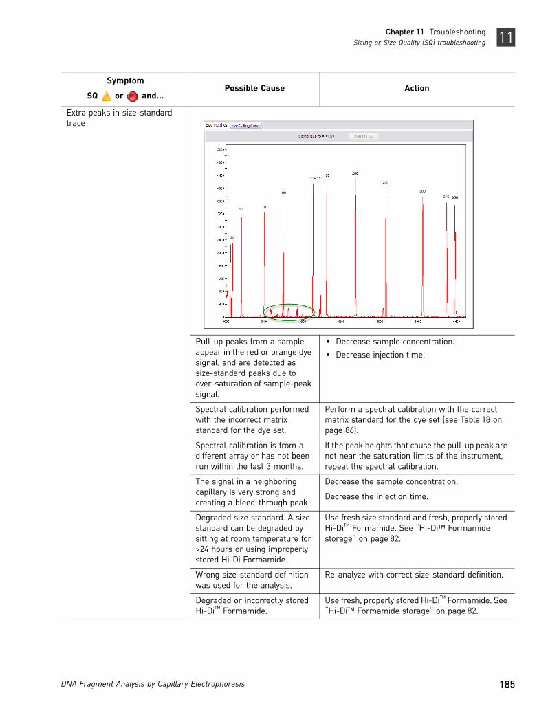
185DNA Fragment Analysis by Capillary Electrophoresis
Chapter 11 TroubleshootingSizing or Size Quality (SQ) troubleshooting 11
Extra peaks in size-standard trace
Pull-up peaks from a sample appear in the red or orange dye signal, and are detected as size-standard peaks due to over-saturation of sample-peak signal.
• Decrease sample concentration.• Decrease injection time.
Spectral calibration performed with the incorrect matrix standard for the dye set.
Perform a spectral calibration with the correct matrix standard for the dye set (see Table 18 on page 86).
Spectral calibration is from a different array or has not been run within the last 3 months.
If the peak heights that cause the pull-up peak are not near the saturation limits of the instrument, repeat the spectral calibration.
The signal in a neighboring capillary is very strong and creating a bleed-through peak.
Decrease the sample concentration.
Decrease the injection time.
Degraded size standard. A size standard can be degraded by sitting at room temperature for >24 hours or using improperly stored Hi-Di Formamide.
Use fresh size standard and fresh, properly stored Hi-Di™ Formamide. See “Hi-Di™ Formamide storage” on page 82.
Wrong size-standard definition was used for the analysis.
Re-analyze with correct size-standard definition.
Degraded or incorrectly stored Hi-Di™ Formamide.
Use fresh, properly stored Hi-Di™ Formamide. See “Hi-Di™ Formamide storage” on page 82.
Symptom
SQ or and...Possible Cause Action

186 DNA Fragment Analysis by Capillary Electrophoresis
Chapter 11 TroubleshootingSizing or Size Quality (SQ) troubleshooting11
Sizing failures occur in a regular pattern (the same wells fail repeatedly)
• Electrophoresis or pipetting error.
• Defective capillaries/arrays.• Autosampler is misaligned.
Refer to the instrument user guide for information on troubleshooting capillaries/arrays.
Noise peaks are detected as size-standard peaks
Contaminated sample. Prepare new sample.
Use fresh, properly stored Hi-Di™ Formamide. See “Hi-Di™ Formamide storage” on page 82.
The Peak Amplitude Threshold of the dye color associated with the size standard is set too high or low in the analysis method.
Adjust the analysis method so that the peak detection threshold associated is greater than the height of the noise signal. See “GeneMapper® Software peak detection settings” on page 94.
Note: You can adjust the threshold if you want to examine the data. However, we recommend that you rerun with increased size-standard concentration.
Size call inaccurate for known DNA sample
Incorrect size standard was added to sample.
Repeat with the correct size standard.
Size standard peaks are not sized correctly.
Examine the size standard peaks and compare the sizes to the size standard definition. See “Viewing the size-standard definition” on page 182.
Migration issues. See “Migration troubleshooting” on page 168.
Symptom
SQ or and...Possible Cause Action
Noise peaks

187DNA Fragment Analysis by Capillary Electrophoresis
Chapter 11 TroubleshootingGeneMapper® Software troubleshooting 11
GeneMapper® Software troubleshooting
Some problems with data can be caused by the settings used to analyze the data. If peak height, morphology, and number of expected peaks are acceptable, but the sample fails sizing, it may be caused by analysis method settings that are not optimized for your application.
For additional troubleshooting information, refer to the GeneMapper® Software Help and the GeneMapper® Software Reference and Troubleshooting Guide (Pub. no. 4403673).
Symptom Possible Cause Action
GeneMapper® Software error message
Generic message - the error for each sample may be different.
View the Info tab (see “Examine the sample info, raw data, and EPT trace” on page 154).
For information on resolving the error, refer to the GeneMapper® Software Reference and Troubleshooting Guide.
Error Message: The bin set in the analysis method does not match the panel used for analysis.
The bin set in the analysis method does not match the panel used for analysis.
Modify the Bin Set selection on the Allele tab in the analysis method.

188 DNA Fragment Analysis by Capillary Electrophoresis
Chapter 11 TroubleshootingGeneMapper® Software troubleshooting11
“al?” label
or alleles are not falling within bins
Allele is migrating at a different rate than expected.
See “Migration troubleshooting” on page 168.
Bin is not defined for the allele.
Modify the binset to define the allele.
Allele not labeled Peak is detected as stutter. Decrease the Stutter ratio in the analysis method.
If the problem persists, mask the stutter peak by labeling the allele as a mono peak: In the Panel Manager, change the marker repeat # to 1 for the marker in question.
Peak intensity is below the Peak Amplitude Threshold in the analysis method.
Adjust the Peak Amplitude Threshold in the analysis method.
Data not sorted by name The default setting in GeneMapper® Software sorts the data by status rather than sample name.
To resort the data:• Select Edit Sort, or • Shift+click the column header to sort by
Clicking once sorts in ascending order, clicking twice sorts in descending order.
When adding samples to a project, the expected data files are not listed in the Add Samples to Project dialog box
Data was not collected as expected.
Ensure the following on the Data Collection Software computer:• The instrument completed the run(s) and data are
visible in Data Collection Software.• Sample files were extracted successfully (3130 Series
or 3730 Series instruments).• The run folder was created and saved on the
instrument computer.• The correct number of *.fsa sample files were created
within the run folder.
Symptom Possible Cause Action

189DNA Fragment Analysis by Capillary Electrophoresis
Chapter 11 TroubleshootingGeneMapper® Software troubleshooting 11
Genotypes tab is grayed
No panel specified before analysis.
Specify a panel in the Project window before analysis.
Two peaks do not separate and are detected as one peak
The software is detecting two separate peaks as one.
Adjust analysis method Peak Detector settings:• Polynomial degree:
A higher setting increases the sensitivity of the curve-fitting process. A lower setting decreases it.
• Peak Window size value:A lower setting increases the sensitivity of the curve-fitting process. A higher setting decreases it.Decrease the peak window size to 13 and re-analyze.
For more information, see “GeneMapper® Software peak detection settings” on page 94.
Symptom Possible Cause Action

190 DNA Fragment Analysis by Capillary Electrophoresis
Chapter 11 TroubleshootingPreamplification gel troubleshooting11
Preamplification gel troubleshooting
Desalting
Impact of high salt concentration
Samples high in salt result in poor injections and low signal intensity. You may be able to compensate for decreased signal intensity by:
• Re‐injecting the sample. Salt preferentially injects smaller fragments and inhibits injection of larger fragments, so the majority of salt may have been injected in the first injection.
• Increasing the injection time and/or injection voltage.
If reinjecting and increasing the injection parameters does not improve signal intensity, desalt and/or concentrate the samples.
Do not increase sample concentration by evaporating the samples without performing a desalting step. Doing so increases the salt concentration and prevents complete denaturation of the DNA which causes decreased signal strength.
Eliminating salt concentration as the cause
To determine if salt concentration is causing low signal intensity, run the size standard alone (see “Running controls to isolate a problem” on page 156). If you see:
• Resolution loss with the size standard, troubleshoot instrument/reagent issue. Refer to the instrument user guide for information.
• No resolution loss with the size standard, add sample to the well containing the size standard and run again. If resolution decreases, desalt the sample.
Desalting To desalt your sample(s), try one of the following:
• NucAway™ Spin Columns—NucAway™ Spin Columns remove unincorporated nucleotides and salts after probe synthesis reactions. Rehydrate the column, centrifuge to remove the interstitial fluid, add the sample to the top of the column, and centrifuge again.
• Amicon Centricon‐100 Microconcentrator (or Centricon‐30 for fragments smaller than 130 bp)
• Ethanol precipitation of the pooled PCR product, followed by resuspension in distilled, deionized water. Refer to Molecular cloning (Sambrook, Fritsch, and Maniatis 1989) for protocols.
• Sample dialysis on a filter membrane:
a. Float a Millipore® VS filter (Millipore Part no. VSWP 02500), shiny side up, on top of 50 mL of deionized, autoclaved water in a 50‐mL conical plastic tube.
b. Carefully spot ~15 μL of sample on top of the filter, using an appropriate pipette.
Symptom Possible Cause Action
No DNA smear on agarose gel (AFLP® only)
Incomplete digestion of DNA.
Check that enzymes are not expired, incubation temperature settings are correct, and so on. Redigest DNA.

191DNA Fragment Analysis by Capillary Electrophoresis
Chapter 11 TroubleshootingEvaluating 310 Genetic Analyzer multicomponent matrix quality 11
c. Dialyze the sample for 20 minutes.
d. Using a pipette, very carefully remove the sample and dilute.
Evaluating 310 Genetic Analyzer multicomponent matrix quality
Purpose of the multicomponent matrix
The multicomponent matrix compensates for the overlap of different dye colors by subtracting out, in each dye’s detection range, the portion of the signal due to fluorescence from other dyes.
Factors affecting matrix quality
• Reagent quality/freshness• Buffer type and concentration• Polymer type• Denaturing or non‐denaturing conditions• Run temperature
When to create a new matrix
When you create a matrix, you must run each dye matrix standard separately to determine the proportional amount of fluorescence that is emitted in all four detection regions.
Because the emission spectra of the dyes vary with the physical environment (such as the pH or polymer type and concentration), create a new matrix if run conditions change.
If you observe any of the symptoms listed in the table on the next page, create a new matrix. You can apply the new matrix to old samples and reanalyze the data.
Virtual Filter Set C Matrix files made for Virtual Filter Set C are especially susceptible to minor changes in run conditions because of the emission maximum of 6‐FAM™ dye (the recommended blue‐displaying dye for this filter set):
• It is very close to the laser wavelength of 514.5 nm. Thus, the window for collected blue light‐intensity data is offset to longer wavelengths and does not contain the emission maximum of 6‐FAM™ dye.
• It is also very close to the detection region for the green‐displaying TET™ dye.
If you are using Virtual Filter Set C, watch for evidence of matrix problems and create a new matrix as soon as problems appear
Identifying matrix problems
A poor or incorrect matrix results in too much or too little subtraction of dye spectral overlap during data analysis. Each causes a recognizable electropherogram anomaly:
• Bleedthrough peaks, also called “pull‐ups”, are caused by too little subtractionBleedthrough peaks are small peaks of one color lying directly under a large peak of another color even though there is no PCR product corresponding to the smaller peak.
• Elevated interpeak baseline is caused by too much subtraction
The table on the next page contains examples of the symptoms listed above.

192 DNA Fragment Analysis by Capillary Electrophoresis
Chapter 11 TroubleshootingEvaluating 310 Genetic Analyzer multicomponent matrix quality11
Symptom Possible Cause Action
Pull-up peaks (too little matrix subtraction)
The matrix was made with the wrong dyes or filter set.
Create a new matrix with the correct dye and filter set. See “Dye sets” on page 41.
The signal from a large peak is off-scale because of sample overloading. In the raw data, the peak showing pull-up is off-scale.
Keep peak heights between approximately 150 and 4000 RFU. If sample data is off-scale, do one of the following:• Rerun the samples using a shorter injection
time.• Dilute and rerun the samples.• Create a new matrix with the correct dye
and filter set. See “Dye sets” on page 41.
Elevated interpeak baseline (too much matrix subtraction)
Too much matrix subtraction Create a new matrix.

193DNA Fragment Analysis by Capillary Electrophoresis
Ordering Information
■ Thermal cyclers and accessories. . . . . . . . . . . . . . . . . . . . . . . . . . . . . . . . . . . . . . . . 193
■ Genetic analyzers and consumables . . . . . . . . . . . . . . . . . . . . . . . . . . . . . . . . . . . . 194
■ GeneScan™ size standards . . . . . . . . . . . . . . . . . . . . . . . . . . . . . . . . . . . . . . . . . . . . 197
■ Matrix standards for spectral calibration . . . . . . . . . . . . . . . . . . . . . . . . . . . . . . . . 197
■ Installation standards. . . . . . . . . . . . . . . . . . . . . . . . . . . . . . . . . . . . . . . . . . . . . . . . . 197
■ Reagent kits . . . . . . . . . . . . . . . . . . . . . . . . . . . . . . . . . . . . . . . . . . . . . . . . . . . . . . . . . 198
■ Other user‐supplied materials . . . . . . . . . . . . . . . . . . . . . . . . . . . . . . . . . . . . . . . . . 198
Thermal cyclers and accessories
Item Source
Veriti® 96-Well Thermal Cycler 4375786
GeneAmp® PCR System 9700 with the Silver 96-Well Block N8050001
GeneAmp® PCR System 9700 with the Gold-plated Silver 96-Well Block 4314878
Silver 96-Well Sample Block N8050251
Gold-plated Silver 96-Well Sample Block 4314443
MicroAmp® Autoclaved Reaction Tubes with Caps, 0.2 mL N8010612
GeneAmp® Autoclaved Thin-walled Reaction Tubes with Domed Caps, 2000 tubes N8010537
GeneAmp® Autoclaved Thin-walled Reaction Tubes with Domed Caps, 1000 tubes N8010611
MicroAmp® 96-Well Tray N8010541
MicroAmp® Reaction Tube with Cap, 0.2-mL N8010540
MicroAmp® 8-Tube Strip, 0.2-mL N8010580
MicroAmp® 8-Cap Strip N8010535
MicroAmp® 96-Well Tray/Retainer Set 403081
MicroAmp® 96-Well Base N8010531
MicroAmp® Clear Adhesive Film 4306311
MicroAmp® Optical Adhesive Film 4311971
MicroAmp® Optical 96-Well Reaction Plate N8010560

194 DNA Fragment Analysis by Capillary Electrophoresis
Ordering Information Genetic analyzers and consumables
Genetic analyzers and consumables
Item† Source
Applied Biosystems® 3500 or 3500xL Genetic Analyzer Contact your local Thermo Fisher Scientific sales representative
Applied Biosystems® 3500xL Genetic Analyzer
3130 or 3130xl Genetic Analyzer
3730 or 3730xl DNA Analyzer
310 Genetic Analyzer
3500/3500xL Analyzer materials
Anode Buffer Container (ABC) 4393927
Cathode Buffer Container (CBC) 4408256
Septa Cathode Buffer Container, 3500 Series 4410715
Conditioning Reagent 4393718
Capillary Array, 36 cm, 8 Capillary, 3500 Genetic Analyzers 4404683
Capillary Array, 50 cm, 8 Capillary, 3500 Genetic Analyzers 4404685
Capillary Array, 36 cm, 24 Capillary, 3500xL Genetic Analyzers 4404687
Capillary Array, 50 cm, 24 Capillary, 3500xL Genetic Analyzers 4404689
GeneScan™ Size Standards See “GeneScan™ size standards” on page 197.
Matrix Standard Kits See “Matrix standards for spectral calibration”
on page 197.
POP-4® Polymer (960 Samples), 3500/3500xL Genetic Analyzers 4393710
POP-4® Polymer (384 Samples), 3500/3500xL Genetic Analyzers 4393715
POP-6™ Polymer (960 Samples), 3500/3500xL Genetic Analyzers 4393712
POP-6™ Polymer (384 Samples), 3500/3500xL Genetic Analyzers 4393717
POP-7™ Polymer (960 Samples), 3500/3500xL Genetic Analyzers 4393710
POP-7™ Polymer (384 Samples), 3500/3500xL Genetic Analyzers 4393715
8-Tube Retainer and Base Set (Standard) for 3500/3500xL Genetic Analyzers 4410231
8-Strip Septa for 3500/3500xL Genetic Analyzers 4410701
96-well Retainer and Base Set (Standard) 3500/3500xL Genetic Analyzers 4410228
96-Well Septa for 3500/3500xL Genetic Analyzers 4412614
3730/3730xl Analyzer materials
Capillary Array, 50 cm, 48 Capillary, 3730 for Genetic Analyzers 4331250
Capillary Array, 36 cm, 48 Capillary, 3730 for Genetic Analyzers 4331247
Capillary Array, 50 cm, 96 Capillary, 3730xl for Genetic Analyzers 4331246
Capillary Array, 36 cm, 96 Capillary, 3730xl for Genetic Analyzers 4331244
GeneScan™ Size Standards See “GeneScan™ size standards” on page 197.

195DNA Fragment Analysis by Capillary Electrophoresis
Ordering InformationGenetic analyzers and consumables
Matrix Standard Kits See “Matrix standards for spectral calibration”
on page 197.
POP-7™ Polymer (28 mL), 3730/3730xl Genetic Analyzers 4363929
POP-7™ Polymer (140 mL), 3730/3730xl Genetic Analyzers 4335615
POP-7™ Polymer (280 mL), 3730/3730xl Genetic Analyzers 4363935
POP-7™ Polymer (840 mL), 3730/3730xl Genetic Analyzers 4335611
MicroAmp® Optical 96-Well Reaction Plate N8010560
Hi-Di™ Formamide 4311320
Reservoir Septa 4315932
Running Buffer, 10✕ 402824
96-Well Plate Septa 4315933
3130/3130xl Analyzer materials
96-Well Plate Septa 4315933
Reservoir Septa 4315932
Capillary Array, 80 cm, 4 Capillary, 3130 Genetic Analyzers 4333465
Capillary Array, 50 cm, 4 Capillary, 3130 Genetic Analyzers 4333466
Capillary Array, 36 cm, 4 Capillary, 3130 Genetic Analyzers 4333464
Capillary Array, 22 cm, 4 Capillary, 3130 Genetic Analyzers 4333463
Capillary Array, 80 cm, 16 Capillary, 3130xl Genetic Analyzers 4319899
Capillary Array, 50 cm, 16 Capillary, 3130xl Genetic Analyzers 4315930
Capillary Array, 36 cm, 16 Capillary, 3130xl Genetic Analyzers 4315931
Capillary Array, 22cm, 16 Capillary, 3130xl Genetic Analyzers 4319898
GeneScan™ Size Standards See “GeneScan™ size standards” on page 197.
Matrix Standard Kits See “Matrix standards for spectral calibration”
on page 197.
POP-4® Polymer (7000 μL), 3130/3300xl Genetic Analyzers 4352755
POP-4® Polymer (3500 μL), 3130/3300xl Genetic Analyzers 4363752
POP-6™ Polymer (7000 μL), 3130/3300xl Genetic Analyzers 4352757
POP-6™ Polymer (3500 μL), 3130/3300xl Genetic Analyzers 4363783
POP-7™ Polymer (7000 μL), 3130/3300xl Genetic Analyzers 4352759
POP-7™ Polymer (3500 μL), 3130/3300xl Genetic Analyzers 4363785
Running Buffer, 10✕ 402824
MicroAmp® Optical 96-Well Reaction Plate N8010560
3100/3100-Avant Genetic Analyzer Autosampler Plate Kit, 96-well 4316471
Hi-Di™ Formamide 4311320
310 Analyzer materials
Item† Source
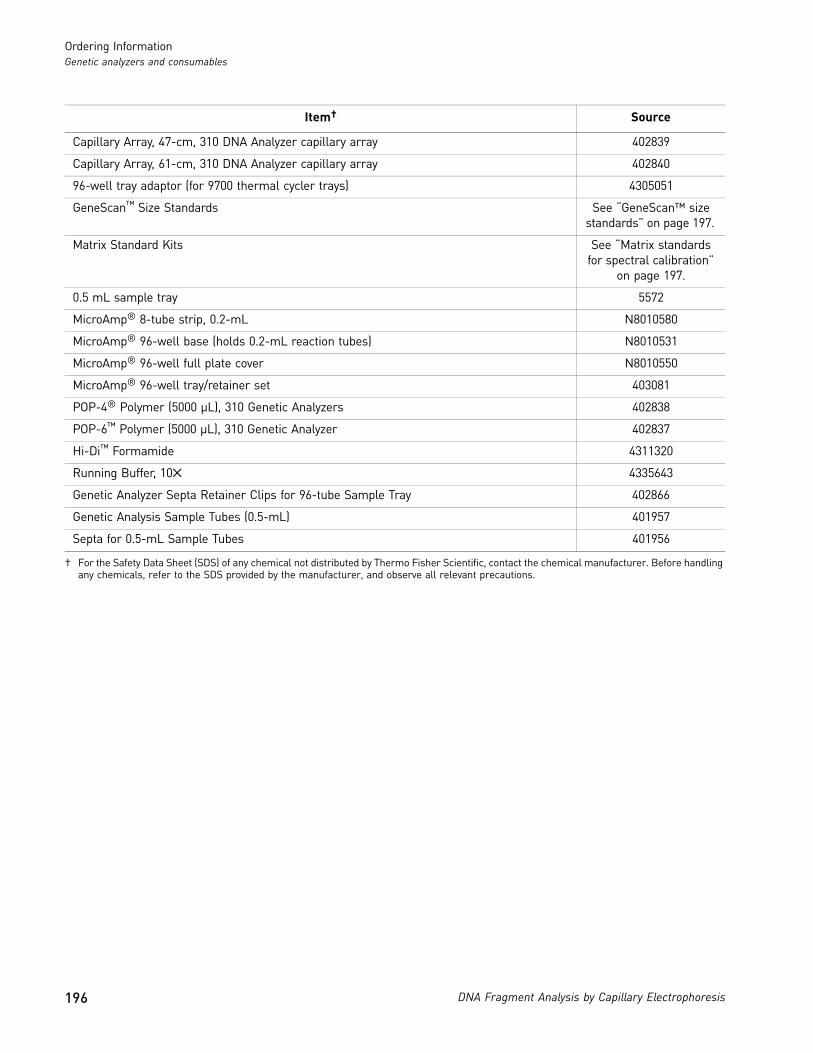
196 DNA Fragment Analysis by Capillary Electrophoresis
Ordering Information Genetic analyzers and consumables
Capillary Array, 47-cm, 310 DNA Analyzer capillary array 402839
Capillary Array, 61-cm, 310 DNA Analyzer capillary array 402840
96-well tray adaptor (for 9700 thermal cycler trays) 4305051
GeneScan™ Size Standards See “GeneScan™ size standards” on page 197.
Matrix Standard Kits See “Matrix standards for spectral calibration”
on page 197.
0.5 mL sample tray 5572
MicroAmp® 8-tube strip, 0.2-mL N8010580
MicroAmp® 96-well base (holds 0.2-mL reaction tubes) N8010531
MicroAmp® 96-well full plate cover N8010550
MicroAmp® 96-well tray/retainer set 403081
POP-4® Polymer (5000 μL), 310 Genetic Analyzers 402838
POP-6™ Polymer (5000 μL), 310 Genetic Analyzer 402837
Hi-Di™ Formamide 4311320
Running Buffer, 10✕ 4335643
Genetic Analyzer Septa Retainer Clips for 96-tube Sample Tray 402866
Genetic Analysis Sample Tubes (0.5-mL) 401957
Septa for 0.5-mL Sample Tubes 401956
† For the Safety Data Sheet (SDS) of any chemical not distributed by Thermo Fisher Scientific, contact the chemical manufacturer. Before handling any chemicals, refer to the SDS provided by the manufacturer, and observe all relevant precautions.
Item† Source

197DNA Fragment Analysis by Capillary Electrophoresis
Ordering InformationGeneScan™ size standards
GeneScan™ size standards
Matrix standards for spectral calibration
Dye sets have been tested and optimized for the instrument, except where noted.
Installation standards
LIZ® dye-labeled size standards
(5-dye chemistry)Part no.
ROX™ dye-labeled size standards
(4-dye chemistry)Part no.
GeneScan™ 120 LIZ® 4324287 GeneScan™ 350 ROX™ 401735
GeneScan™ 500 LIZ®† 4322682 GeneScan™ 400HD ROX™ 402985
GeneScan™ 600 LIZ® 4366589 GeneScan™ 500 ROX™† 401734
GeneScan™ 600 LIZ® v2.0† 4408399 GeneScan™ 1000 ROX™‡ 401098
GeneScan™ 1200 LIZ®† 4379950 — —
† For denaturing and non-denaturing applications.‡ For non-denaturing applications only.
InstrumentsDye Set part numbers
DS-02 DS-20† DS-30 DS-31 DS-32 DS-33 DS-34
3500 Series 4323014 Not tested
4345827† 4345829† 4345831 4345833 Not tested
3730 Series 4323014‡ Not tested
4345827† 4345829† 4345831† 4345833 Not tested
3130 Series 4323014 Not tested
434445827 4345829 4345831 4345833 Not tested
310 4323050 401114 401546, 402996
401546, 402996, 4313939
4312131 4318159 401546
† Dye primer matrix standards.‡ We have tested this dye set but have not optimized for this instrument.
Installation standard Source For use with
DS-33 GeneScan™ Installation Standards 4376911 GeneScan™ 600 LIZ® Size Standard v2.0 (6-FAM™, VIC®, NED™, and PET® dyes)
DS-33 GeneScan™ Installation Standards 4330397 GeneScan™ 500 LIZ® Size Standard (6-FAM™, VIC®, NED™, and PET® dyes)
DS-30 GeneScan™ Installation Standards 4316144 GeneScan™ 500 ROX™ (6-FAM™, HEX™, and NED™ dyes)

198 DNA Fragment Analysis by Capillary Electrophoresis
Ordering Information Reagent kits
Reagent kits
Other user-supplied materials
Item† Source
AFLP® Kits
AFLP® I Selective Primer Kit 4303050
AFLP® II Selective Primer Kit 4303051
AFLP® EcoRI Ligation/Amplification Module 402941
AFLP® MseI Ligation/Amplification Module 402942
AFLP® Amplification Core Mix Module 402005
SNaPshot® Kits
SNaPshot® Multiplex Kit Contact your local representative
SNaPshot® Primer Focus® Kit 4329538
GeneAmp® EZ rTth RNA PCR Kit N808-0178
GeneAmp® PCR Carryover Prevention Kit N808-0068
AmpErase® UNG N808-0096
† For the Safety Data Sheet (SDS) of any chemical not distributed by Thermo Fisher Scientific, contact the chemical manufacturer. Before handling any chemicals, refer to the SDS provided by the manufacturer, and observe all relevant precautions.
Item† Source
Hi-Di™ Formamide, 25-mL 4311320
Aerosol resistant pipette tips MLS
Microcentrifuge tubes MLS
Pipettors MLS
Tape, labeling MLS
Tube, 50-mL Falcon MLS
Tube decapper, autoclavable MLS
Deionized water, PCR grade MLS
Vortex MLS
Millipore® VS filter Millipore Part no. VSWP 02500
CEPH Individual 1347-02 Control DNA 403062
† For the Safety Data Sheet (SDS) of any chemical not distributed by Thermo Fisher Scientific, contact the chemical manufacturer. Before handling any chemicals, refer to the SDS provided by the manufacturer, and observe all relevant precautions.

199DNA Fragment Analysis by Capillary Electrophoresis
Documentation and Support
The publication numbers in this section are for the latest product versions available at the time of publication. For documentation for newer product versions, go to www.lifetechnologies.com.
Instrument documentation
GeneMapper® Software documentation
Document Publication number
Applied Biosystems® 3500/3500xL Genetic Analyzer User Guide (3500 Series Software v1.0) 4401661
Applied Biosystems® 3500/3500xL Specification Sheet 106SP11-01
Applied Biosystems® 3730 DNA Analyzer Getting Started Guide 4359476
Applied Biosystems® 3730/3730xl DNA Analyzer Specification Sheet 106SP08-01
Applied Biosystems® 3130/3130xl Genetic Analyzers Getting Started Guide 4352715
Applied Biosystems® 3130/3130xl Specification Sheet 106SP07-03
310 Genetic Analyzer User Guide 4317588
310 Genetic Analyzer Specification Sheet 903565
Veriti® Thermal Cycler User Guide 4375799
GeneAmp® PCR System 9700 User Guide 4303481
Document Publication number
GeneMapper® Software Getting Started Guide: AFLP® System Analysis 4403620
GeneMapper® Software Getting Started Guide: Loss of Heterozygosity (LOH) Analysis 4403621
GeneMapper® Software Getting Started Guide: Microsatellite Analysis 4403672
GeneMapper® Software Getting Started Guide: SNaPshot® Kit Analysis 4403618
GeneMapper® Software Reference and Troubleshooting Guide 4403614
GeneMapper® Software Installation and Administration Guide v4.1 4403614
GeneMapper® Software Reference and Troubleshooting Guide v4.1 4403673
GeneMapper® Software Quick Reference Guide v4.1 4403615

200 DNA Fragment Analysis by Capillary Electrophoresis
Documentation and Support Peak Scanner Software documentation
Peak Scanner Software documentation
Application documentation
Document Publication number
Peak Scanner Software Reference Guide 4382253
Peak Scanner Software Quick Reference Card 4383719
Document Publication number
AFLP® applications
GeneMapper® Software Getting Started Guide: AFLP® System Analysis 4403620
AFLP® Microbial Fingerprinting Protocol 402977
AFLP® Plant Mapping Protocol 4303146
Aneuploidy applications
Aneuploidy Detection by QF-PCR of STR Markers on the Applied Biosystems® 3500xL Genetic Analyzer 106AP28-01
BAC applications
BAC Fingerprinting on the Applied Biosystems® 3730/3730xl DNA Analyzer 107AP04-01
Sizing of Large DNA Fragments Generated by BAC Fingerprinting on Capillary Electrophoresis System 106AP25-01
HiCEP applications
High coverage gene expression profiling on the Applied Biosystems® 3500xL Genetic Analyzer CO15884
ISSR applications
ISSR Genotyping of Endangered Plants Using an Optimized Workflow 106AP31-01
LOH applications
GeneMapper® Software Getting Started Guide: Loss of Heterozygosity (LOH) Analysis 4403621
Relative Fluorescent Quantitation on CapillaryElectrophoresis Systems: Screening for Loss of Heterozygosity in Tumor Samples on the Applied Biosystems® 3130 Series Genetic Analyzers with GeneMapper® Software v3.7
106AP15-01
Methylation applications
Cells-to-CpG™ Bisulfite Conversion Kit (50) Protocol 4448998
Advances in Capillary Electrophoresis-Based Methods for DNA Methylation Analysis 106BR14-01
Three Optimized Workflows for CpG Island Methylation Profiling 106AP24-01
Microsatellite applications
GeneMapper® Software Getting Started Guide: Microsatellite Analysis 4403672
Fact sheet: Microsatellite Analysis on the Applied Biosystems® 3130 Series Genetic Analyzers 106MI61-01
Uniparental disomy (UPD) analysis of chromosome 15 CO18249
Relative fluorescence quantitation applications
Aneuploidy Detection by QF-PCR of STR Markers on the Applied Biosystems® 3500xL Genetic Analyzer 106AP28-01

201DNA Fragment Analysis by Capillary Electrophoresis
Documentation and SupportObtain SDSs
Obtain SDSs
Safety Data Sheets (SDSs) are available from www.lifetechnologies.com/support.
Note: For the SDSs of chemicals not distributed by Thermo Fisher Scientific, contact the chemical manufacturer.
Obtain support
For the latest services and support information for all locations, go to:
www.lifetechnologies.com/support
At the website, you can:
• Access worldwide telephone and fax numbers to contact Technical Support and Sales facilities
• Search through frequently asked questions (FAQs)• Submit a question directly to Technical Support• Search for user documents, SDSs, vector maps and sequences, application notes,
formulations, handbooks, certificates of analysis, citations, and other product support documents
• Obtain information about customer training• Download software updates and patches
Relative Fluorescent Quantitation on Capillary Electrophoresis Systems: Screening for Loss of Heterozygosity in Tumor Samples on the Applied Biosystems® 3130 Series Genetic Analyzers with GeneMapper® Software v3.7
106AP15-01
SNP applications
GeneMapper® Software Getting Started Guide: SNaPshot® Kit Analysis 4403618
User Bulletin: Using the SNaPshot® Multiplex System with the POP-7™ Polymer on Applied Biosystems® 3730/3730xl DNA Analyzers and 3130/3130
4367258
SNaPshot® Multiplex Kit Quick Reference Card 4323975
Demonstration of SNP Genotyping Using a Single Nucleotide Extension Method and the 3500 Series Genetic Analyzer
CO12863
Using the SNaPshot® Multiplex System with the POP-7™ Polymer on Applied Biosystems® 3730/3730xl DNA Analyzers and 3130/3130xl Genetic Analyzers
4367258
Document Publication number

202 DNA Fragment Analysis by Capillary Electrophoresis
Documentation and Support Obtain support

203DNA Fragment Analysis by Capillary Electrophoresis
References
Ammiraju, J.S.S., Dholakia, B.B., Santra, D.K. et al. 2001. Identification of inter simple sequence repeat (ISSR) markers associated with seed size in wheat. Theor Appl Genet. 102:726–732.
Andersen, P.S., Jespersgaard, C., Vuust, J. et al. 2003.Capillary electrophoresis‐based single strand DNA conformation analysis in high‐throughput mutation screening. Hum Mutat. 21:455–465.
Anderson, G.R., Brenner, B.M., Swede, H. et al. 2001. Intrachromosomal genomic instability in human sporadic colorectal cancer measured by genome‐wide allelotyping and inter‐(simple sequence repeat) PCR. Cancer Res. 61:8274–8283.
Blair, M.W., Panaud, O., McCouch, S.R. 1999. Inter‐simple sequence repeat (ISSR) amplification for analysis of microsatellite motif frequency and fingerprinting in rice (Oryza sativa L.). Theor Appl Genet. 98:780–792.
Canzian, F. Salovaara, R., Hemminki, A. et al. 1996. Semiautomated Assessment of Loss of Heterozygosity and Replication Error in Tumors. Cancer Res. 56:3331–3337.
Davis, L.M., Glenn, T.C., Strickland, D.C. et al. 2002. Microsatellite DNA analyses support an east‐west phylogeographic split of American alligator populations. J Exp Zool. 294:352–72.
Derakshani, M., Lukow, T. and Liesack, W. 2001. Novel bacterial lineages at the (sub) division level as detected signature nucleotide targeted recovery of 16s rRNA genes from bulk soil and rice roots of flooded rice microcosms. Applied Environmental Microbiology. 67(2):623–631.
Doyle, J.J., Doyle J.L. 1987. A rapid DNA isolation procedure for small quantities of fresh leaf tissue. Phytochem Bull. 19:11–15.
Ellegren, H. 2004. Microsatellites: simple sequences with complex evolution. Nat Rev Genet. 5:435–45.
Eschenhagen, M., Schuppler, M., and Roske, I. 2003. Molecular characterization of the microbial community structure in two activated sludge systems for the advanced treatment of domestic effluents. Water Res. 37(13):3224–3232.
Fleischer, R.C. and Lowe, S. 1995. Construction and screening of microsatellite‐enrichedgenomic libraries. In Ferraris, J. and Palumbi, S. (eds), Molecular Zoology: Advances, Strategies and Protocols. Wiley‐Liss, NY, 459–468.
Goel, S., Chen, Z., Akiyama, Y., Connor, J.A., et al. 2006. Comparative physical mapping of the apospory‐specific genomic region in two apomictic grasses: Pennisetum squamulatum and Cenchru sciliaris. Genetics. 173(1):389–400.
Gupta, S.K., Souframanien, J., and Gopalakrishna, T. 2008. Construction of a genetic linkage map of black gram, Vigna mungo (L.) Hepper, based on molecular markers and comparative studies. Genome. 51:628–637.

204 DNA Fragment Analysis by Capillary Electrophoresis
References
Hauge, X.Y., and Litt, M. 1993. A study of the origin of ʹshadow bandsʹ seen when typing dinucleotide repeat polymorphisms by the PCR. Hum Mol Genet. 2:411–415.
Holleley, C.E., and Geerts, P.G., 2009. Multiplex Manager 1.0: a cross‐platform computer program that plans and optimizes multiplex PCR. BioTechniques 46:511‐517.
Huelsenbeck, J.P., and Ronquist, F. 2001. MRBAYES: Bayesian inference of phylogeny. Bioinformatics 17:754–755.
Inazuka, M., Tahira, T., and Hayashi, K. 1996. One‐tube post‐PCR fluorescent labeling of DNA fragments. Genome Res. 6:551–557.
Inazuka, M., Wenz, H.M., Sakabe, M., Tahira, T., and Hayashi, K. 1997. A streamlined mutation detection system: multicolor post‐PCR fluorescence labeling and single‐strand conformational polymorphism analysis by capillary electrophoresis. Genome Res. 7:1094–1103.
Iwahana, H., Adzuma, K., Takahashi, Y., Katashima, R., Yoshimoto, K., and Itakura, M. 1995. Multiple fluorescence‐based PCR‐SSCP analysis with postlabeling. Genome Res. 4:275–282.
Johnson, E.L., Zhang, D., Emche, S.D. et al. 1994. Construction of libraries enriched for sequence repeats and jumping clones, and hybridization selection for region‐specific markers. Proc Natl. Acad. Sci. USA 91:88–92.
Lai, Y. and Sun, F., The relationship between microsatellite slippage mutation rate and the number of repeat units. 2003. Molecular Biology and Evolution. 20(12):2123–2131.
Leroy, X.J., and Leon, K. 2000. A rapid method for detection of plant genomic instability using unanchored‐microsatellite primers. Plant Mol Biol Rep. 2000. 18:283a–283g.
Luo, M.C. et al., High‐throughput fingerprinting of bacterial artificial chromosomes using the SNaPshot® labeling kit and sizing of restriction fragments by capillary electrophoresis, Genomics 82 (2003) 378–389.
Molecular Cloning. 1987. Second Edition. Cold Spring Harbor Laboratory, NY: Cold Spring Harbor Laboratory Press.
Murray, V., Monachawin, C., and England, P.R. 1993. The determination of the sequences present in the shadow bands of a dinucleotide repeat PCR. Nucleic Acids Research. 21:2395–2398.
Orita, M., Iwahana, H., Kanazawa, H. et al. 1989. Inter‐ and Intra‐specific Variation among Five Erythroxylum Taxa Assessed by AFLP. Proc Natl Acad Sci USA 86:2766–2770.
Osborn, A. M., Moore, R.B., and Timmis, K.N. 2000. An evaluation of terminal‐restriction fragment length polymorphism (T‐RFLP) analysis for the study of microbial community structure and dynamics. Environmental Microbiology. 2(1): 39–50.
Naimuddin, M. and Nishigaki, K. 2004. Genome analysis technologies: Towards species identification by genotype. Briefings in Functional Genomics and Proteomics 1(4):356–371.
Ronquist, F., and Huelsenbeck, J.P. 2003. MRBAYES 3: Bayesian phylogenetic inference under mixed models. Bioinformatics 19:1572–1574.

205DNA Fragment Analysis by Capillary Electrophoresis
References
Sakamoto, M., Takeuchi, Y., Umeda, M., Ishikawa, I. and Benno, Y. 2003. Application of terminal RFLP analysis to characterize oral bacterial flora in saliva of healthy subjects and patients with periodontitis. J Med Microbiol. 52:79–89.
Savelkoul, P.H.M., Aarts, H.J.M., de Haas, J. et al. 1999. Amplified‐fragment length polymorphism analysis: the state of an art. J Clin Microbiol. 37(10)3083–3091.
Serra, R., Cabanes, F.J., Perrone, G., Venancio, A., Mule, G., and Kozakiewicz, Z. 2006. Aspergillus ibericus: a new species of section Nigri isolated from grapes. Mycologia 98(2)295–306.
Shihabi, Z. K. and Hinsdale, M. E. 1995. Some variables affecting reproducibility in capillary electrophoresis. Electrophoresis. 16: 2159–2163.
Shinde, D., Lai, Y., Sun, F., and Arnheim, N. 2003. Taq DNA polymerase slippage mutation rates measured by PCR and quasi‐likelihood analysis: (GA/GT)n and (A/T)n microsatellites. Nucleic Acids Res. 31:974–980.
Topal, M.D., and Fresco, J.R. 1976. Complementary base pairing and the origin of substitution mutations. Nature 263:285–289.
UBC Primer Set 9, 2006. www.michaelsmith.ubc.ca/services/NAPS/Primer_Sets/ Primers_Oct2006.pdf
Wan Q‐H., Wu, H., Fujihara, T., and Fang, S‐G. 2004. Which genetic marker for which conservation genetics issue? Electrophoresis. 25:2165–2176.
Wang, H.Z., Wu, Z.X., Lu, J.J. et al. 2009. Molecular diversity and relationships among Cymbidium goeringii cultivars based on inter‐simple sequence repeat (ISSR) markers. Genetica 136:391–399.
Witmer, P. D., Doheny, K.F., Adams, M.K., Boehm, C.D. et al., 2003. The development of a highly informative mouse simple sequence length polymorphism (SSLP) marker set and construction of a mouse family free using parsimony analysis. Genome Res. 13:485–491.
Wolfe, A.D., Xiang, Q‐Y., and Kephart, S.R. 1998. Assessing hybridization in natural populations of Penstemon (Scrophulariaceae) using hypervariable inter simple sequence repeat markers. Mol Ecol. 71:1107–1125.
Zhao, H., Bughrara, S.S., and Oliveira, J.A. 2006. Genetic diversity in colonial bentgrass (Agrostis capillaris L.) revealed by EcoRI‐MseI and PstI‐MseI AFLP markers. Genome. 49(4):328–335.

206 DNA Fragment Analysis by Capillary Electrophoresis
References

207DNA Fragment Analysis by Capillary Electrophoresis
Glossary
allele One specific sequence of a locus. Different alleles of a single locus will have slightly different DNA sequences.
amplicon The product of a PCR reaction. Typically, an amplicon is a short piece of DNA.
association studies Studies that interrogate a dense set of markers to identify associations between those markers and the loci of interest. Association studies are more powerful than linkage mapping studies for the detection of weak‐susceptibility loci.
backcross A genetic cross where an individual from the F1 generation is mated to an individual with the genotype of one of the parents.
bin In GeneMapper® Software, the expected location of an individual peak or allele, defined by a base‐pair range and a color. You typically define a bin for each possible allele associated with a marker.
binset In GeneMapper® Software, a set of bins that you specify in the analysis method.
contig In BAC fingerprinting, a contiguous sequence of DNA created by assembling overlapping sequenced fragments of a chromosome. A group of clones representing overlapping regions of the genome.
diploid Having two copies of every chromosome.
dye set The term “dye set” corresponds to:
• The physical dye set used for labeling fragments.• The software selection you make that identifies the dye colors in the dye set, the
order of the dye peaks in the dye set, and spectral analysis parameters for the dyes.
electrophoresis The act of applying an electrical field to a porous substrate in order to separate molecules by size or shape. For example, nucleic acids like DNA and RNA are negatively charged and are thus attracted to a positive charge and will move toward it through a matrix like a polymer or agarose gel. The strength of the electrical field and charge on the molecules and the size of the pores in the matrix determine the speed at which different molecules in the starting mixture migrate. In general, smaller molecules migrate faster than larger molecules because they are less obstructed as they travel through the matrix.
emission spectrum The intensity of emitted light (fluorescence) as a function of the wavelength of the emitted light.

208 DNA Fragment Analysis by Capillary Electrophoresis
Glossary
excitation efficiency The probability that it will absorb light of a certain wavelength, as a percentage of the probability of absorption at the wavelength of maximum absorption.
excitation spectrum The intensity of emitted light as a function of the wavelength of the exciting light.
filter set Physical filters that separate dye signals in older gel‐based capillary electrophoresis instruments. Newer Thermo Fisher Scientific instruments use a diffraction grating.
fingerprint A characteristic pattern of peaks or bands after an amplification or digest of genomic DNA that can be used to identify an individual.
genetic mapping Analysis of the progeny from genetic crosses to determine the relative position of chromosomal locations.
Linkage mapping A meiotic mapping technique which searches for linkage between a marker and the disease gene within several generations of affected families. These studies examine the inheritance of markers in both affected and unaffected members of the family and then determine whether particular markers are physically close to the disease gene of interest. Linkage mapping can be used to scan the entire genome relatively easily.
ISSR PCR Inter‐simple sequence repeat PCR. See “Inter‐simple sequence repeat (ISSR) PCR” on page 137.
locus A location on a chromosome. The term is sometimes used more narrowly to describe the location of a gene or genetic marker. (Plural: loci). See also Marker.
marker Any observable genetic characteristic (for example, gene, phenotype, microsatellite sequence, SNP) that can be used to identify a genetic location. To be useful in genetic studies, a marker must be present in different forms to allow researchers to distinguish between individuals. One marker represents one locus and one primer pair. Defined by size range of expected alleles and dye (color) attached to primer.
microsatellites Highly repetitive simple sequence repeats of 2 to 7 base pairs, also called short tandem repeats (STRs). Microsatellites fall into the broader category referred to as variable number of tandem repeats (VNTRs), which also includes minisatellites.
minisatellites Highly repetitive simple sequence repeats ranging from approximately 10 to 30 base pairs. Minisatellites fall into the broader category referred to as variable number of tandem repeats (VNTRs), which also includes microsatellites.
panel In GeneMapper® Software, a collection of expected size ranges and dye colors (markers) associated with each primer pair.
phylogenetic studies Studies to determine evolutionary relationships between organisms (for example, species or populations).
polymerase An enzyme that catalyzes polymerization. DNA and RNA polymerases build single‐stranded DNA or RNA (respectively) from free nucleotides, using another single‐stranded DNA or RNA as the template.
polymorphic locus A locus with more than one allele that is commonly found in a population.

209DNA Fragment Analysis by Capillary Electrophoresis
Glossary
population study A study that types genetic markers on a large population to identify associations between a marker and a phenotype.
primer A short single strand of DNA that serves as the priming site for DNA polymerase in a PCR reaction.
pull-up peaks Artifact peaks in one or more dye colors that are caused by high or saturated signal intensity in another dye color.
quantum yield The probability that a dye in its excited state will emit a photon as it decays back to the ground state.
restriction enzymes Endonucleases that cleave the phosphate backbone of double‐stranded DNA at highly specific sequences called restriction sites.
template In PCR, the nucleic acid molecule that provides the sequence to amplify. For example, genomic DNA can be the template for a PCR reaction that amplifies a specific region within the genome.
Variable Number Tandem Repeat (VNTR)
Any genes whose alleles contain different numbers of tandemly repeated oligonucleotide sequences.

210 DNA Fragment Analysis by Capillary Electrophoresis
Glossary

211DNA Fragment Analysis by Capillary Electrophoresis
Index
Numerics2720 Thermal Cycler 583’ A nucleotide addition 33310 instrument
See also capillary electrophoresisdye sets and matrix standards 86matrix, overview 87run module, updating for GeneScan LIZ Size
Standard 46safety information 68signal intensity range 77, 158specifications 68
3130 Series instrumentSee also capillary electrophoresisdye sets and matrix standards 86run module, updating for GeneScan LIZ Size
Standard 48run modules, downloading 48safety information 68signal intensity range 77, 158specifications 68
3500 Series instrumentSee also capillary electrophoresisdye sets and matrix standards 86performance 70run modules 69safety information 68signal intensity range 77, 158specifications 68
3730 Series instrumentSee also capillary electrophoresisdye sets and matrix standards 86run module, downloading 48run module, optimizing for GeneScan 600 LIZ Size
Standard 48run modules 69safety information 68signal intensity range 77, 158specifications 68throughput 69
AAccuPrime Taq DNA Polymerase 22, 24AccuPrime Taq DNA Polymerase High Fidelity 22AFLP
advantages 126analysis method, GeneMapper Software 129applications 127data analysis 129example data 129experiment and primer design
recommendations 127genotypes in GeneMapper Software 130instrument and consumable
recommendations 127overview 125PCR kits 198principle 126restriction enzymes 128workflow 128
agarose gel, using for troubleshooting 157ambient temperature, problems caused by 160amplification
See also PCRnon‐specific 32post‐amplification manipulations 33selective 31
amplified fragment length polymorphism. See AFLPAmpliTaq DNA Polymerase 22, 24AmpliTaq DNA Polymerase, LD 22, 24AmpliTaq Gold DNA Polymerase 23, 24analysis software 89aneuploidy, relative fluorescence application 17animal breeding, microsatellite application 16animal typing, microsatellite application 16annealing temperature
optimizing 64PCR parameters for unknown 61, 63
annealing, factors affecting 30association studies 110autosampler, problems caused by misalignment 161

212 DNA Fragment Analysis by Capillary Electrophoresis
Index
BBAC fingerprinting
applications 133data analysis 73, 90, 159experiment and primer design
recommendations 134instrument and consumable
recommendations 134overview 132principle 133workflow 135
bacterial artificial chromosome. See BAC fingerprint‐ing
baseline troubleshooting 178base‐pairing energies 30, 31bleed‐through peaks. See pull‐up peaksbreeding 110
Ccancer progression analysis 110capillary array
for each instrument 68problems caused by degraded or clogged 160
capillary electrophoresisSee also 310 instrument; 3130 Series
instrument; 3500 Series instrument; 3730 Series instrument
control DNA 57definition 18factors affecting 82injection time, optimizing 79injection voltage, optimizing 80optimizing 67optimizing conditions 80polymers 83run modules 46run time, optimizing 81run voltage, optimizing 81signal intensity 77spatial calibration 84spectral calibration 84troubleshooting 180
CE. See capillary electrophoresisCEPH 1347‐02 Control DNA 57, 157CNV, relative fluorescence application 17concentration
DNA template 59dNTP 59
enzyme 60Mg ion 59sample 158
controlsCEPH 1347‐02 Control DNA 157control DNA, using 57DNA template 157process 157recommendation for frequency 69, 156running to isolate a problem 156
Copy Number Variation. See CNVcustom primer design 29
Ddata
checking quality 104, 153electropherogram quality requirements 104troubleshooting 153
data analysisGeneMapper Software 89Peak Scanner Software 92
desalting 190dinucleotide repeats 115DNA methylation 149DNA polymerase enzymes
3’ A addition 33characteristics 24recommended 22
DNA templateconcentration 59control 157isolating 55purifying 56quantifying 56storing 56
dye setsdye components 41matrix standards for 86
dyeschemical forms 36emission 38emission max 38
Eelectropherogram, quality 104electrophoresis. See capillary electrophoresisEPT trace

213DNA Fragment Analysis by Capillary Electrophoresis
Index
examining 155example of good‐quality 155troubleshooting 180
error message, GeneMapper Software 154evaluating data
electropherogram 104stutter 113
excitation and emission max 38experimental design considerations 21
Ffingerprinting
AFLP 125applications 17BAC 132HiCEP 136ISSR 137T‐RFLP 131
fluorescent labeling 25forensics. See Human Identificationfragment analysis
applications 16definition 15workflow 19
GGeneAmp® Gold Fast PCR Master Mix 23GeneAmp® PCR System 9700, 384‐Well Dual
Autolid 58GeneAmp® PCR System 9700, Dual 384‐well 58GeneAmp® PCR System 9700, Dual 96‐Well 58GeneMapper Software
AFLP default method 129AFLP genotypes 130autoanalysis 91error message 154features 91ISSR bins 139microsatellite default method 112peak detection settings 94peak start and end settings 97sizing 98sizing methods 100SNaPshot default method 123troubleshooting 187workflow 93
general PCR, thermal cycler parameters 61, 62
GeneScan size standards. See size standardgenetic analyzer. See 310 instrument; 3130 Series
instrument; 3500 Series instrument; 3730 Se‐ries instrument
genetic diversityfingerprinting application 17microsatellite application 16
genetic maps for new species, fingerprinting application 17
genome scans 110guidelines
PCR contamination 64PCR parameters 63primer design 29size‐calling 90
Hhairpin secondary structures 31HiCEP 136
applications 136overview 136principle 136workflow 136
HID. See Human IdentificationHi‐Di formamide
issues caused by improperly stored 159storage conditions 82
high coverage expression profiling. See HiCEPhot‐start PCR
description 60enzyme 23thermal cycler parameters 60, 62
Human Identification applications. Go to lifetechnolo‐gies.com
humidity, problems caused by 161
Iinjection
factors affecting 78time, optimizing 79voltage, optimizing 80
instrumentsfor use with guide 13plate types 58problems caused by 160RFU ranges 158run modules 46signal intensity ranges 158

214 DNA Fragment Analysis by Capillary Electrophoresis
Index
troubleshooting 158, 159, 180Inter‐simple sequence repeat. See ISSRionic strength of buffer 78ISSR
applications 138creating multiple bins 139data analysis 139example data 140experiment and primer design
recommendations 139microsatellite application 16overview 137principle 137workflow 139
Llabeling, fluorescent 25laboratory water, problems caused by
contamination 159linkage groups among crosses, fingerprinting
application 17linkage mapping
fragment analysis 16microsatellite analysis 110thermal cycler parameters 62
LOHmicrosatellite application 16relative fluorescence applications 17
Loss of Heterozygosity. See LOHlow‐copy amplification, enzyme 22, 23
Mmatrix
310 instrument 191standards for spectral calibration 86
methylation assessment 149microbial genemapping, fingerprinting
application 17microsatellite analysis
advantages 108applications 110data analysis 112experiment and primer design
recommendations 111instrument and consumable
recommendations 111overview 107principle 108
size standard, GeneScan 400 HD ROX 49size standard, GeneScan 600 LIZ 111stutter 113troubleshooting 113workflow 112
microsatellite instability, microsatellite application 16, 146
migration troubleshooting 168MLPA, relative fluorescence applications 17, 143MLVA, microsatellite application 16multicomponent analysis 26, 37Multilocus Variant Analysis. See MLVAmultiplexing
benefits and limitations 26guidelines 28pooling ratios 27software 28strategies 27troubleshooting 29
Nnoise, troubleshooting 178normalization size standard 45
Pparentage analysis 110paternity testing 110pathogen sub‐typing, microsatellite application 16PCR
See also thermal cycler parameters3’ addition 33carryover 65contamination 64control DNA 57DNA template 55general 61, 62hot‐start 60, 62linkage mapping 62maximize yield of specific products 61, 63non‐specific amplification 32plates 58post‐amplification manipulations 33primer design 29primers, preparing 57problems caused by expired reagents 159products, storing 56reaction volume 58

215DNA Fragment Analysis by Capillary Electrophoresis
Index
reagent concentrations 59selective amplification 31setup 64side reactions 60template volume 58time‐release 61, 62touchdown 61, 63troubleshooting 176XL 63
PCR work areas 64peak detection
peak window size 94polynomial degree 94
peak morphology troubleshooting 169Peak Scanner Software
features 92overview 92
phylogenetic studies 110plant genome mapping, fingerprinting application 17plant typing, microsatellite application 16Platinum Multiplex PCR Master Mix 23, 24Platinum Pfx DNA Polymerase 23, 24polymer
characteristics 83handling 83problems caused by degraded or expired 159types 83
polymerase enzymes. See DNA polymerase enzymespolynomial degree
peak detection 94varying 95window size value 96
pooling ratios for multiplexing 27POP polymer. See polymerpopulation genetics studies 110post‐amplification manipulations 33preamplification troubleshooting 190primer/dimer
minimizing 62primer/dimer, minimizing 60primers
design guidelines 29reconstituting 57SNaPshot 123tailing 34
QQF‐PCR, relative fluorescence applications 17, 143Qualitative Fluorescence PCR. See QF‐PCRquantification
DNA template 56primers 57
Quantitative Multiplex PCR of Short Fluorescent Frag‐ments. See QMPSF
Rraw data
examine 154example 155
reagent troubleshooting 158, 159Relative Fluorescence Quantitation. See RFQReplication error 146RER 146resolution
definition of 79formula 79troubleshooting 169
RFQapplications 17, 144data analysis 145determining relative number of molecules 146determining relative quantities 145experiment and primer design
recommendations 144LOH workflow 145minimizing signal intensity variation 144overview 143peak height versus area 143
RFU ranges for instruments 158rTth DNA polymerase
description 24thermal cycler parameters 63XL 24
run modules 46
SSafety Data Sheets (SDSs), obtaining 201safety information 55salt concentration
desalting 190impact on electrophoresis 82
sampleconcentration, problems caused by high 158

216 DNA Fragment Analysis by Capillary Electrophoresis
Index
contamination, problems caused by 158sample salt concentration. See salt concentrationsecondary structure
primer 30template 31
selective amplification 31signal intensity
minimizing variation 144optimizing 77range for each instrument 77, 158relative order of dyes 38troubleshooting 164
Single Nucleotide Polymorphism. See SNPsingleplexing 26Size Match Editor, displaying 153size methods, GeneMapper Software 100size standards
function 42GS1000 ROX 51GS120 LIZ 44GS1200LIZ 47GS350 ROX 49GS400HD ROX 49GS500 LIZ 44GS500 ROX 50GS600 LIZ 45GS600 LIZ v2.0 45modifying definition 153normalization 45preparation 43storage 43troubleshooting 182
size‐calling guidelines 90sizing
Cubic Spline method 101curve 100Global Southern method 103how the GeneMapper Software performs 98Least Squares method 100Local Southern method 102methods 100troubleshooting 153, 182
sizing qualitychecking 153troubleshooting 182
software, analysis 89spatial calibration, overview 84spectral calibration
matrix standards 41overview 84
split peaks, incomplete 3’ A addition 33SQ. See sizing qualitystandards
See also size standards 42install standard for troubleshooting 157matrix for spectral calibration 86
stutteridentifying 113troubleshooting 113
SuperScript III Reverse Transcriptase 23, 24support, obtaining 201
Ttailing primer 34technical support 201template
DNA 56, 59small volume 58
terminal restriction fragment length polymorphism. See T‐RFLP
thermal cycler parametersgeneral PCR 61, 62hot‐start 60, 62linkage mapping 62optimizing 63time‐release PCR 61, 62touchdown PCR 61, 63XL PCR 63
thermal cyclersapplications 58safety information 55specifications 58
time‐release PCRenzyme 23thermal cycler parameters 61, 62
Tmcalculator 29factors affecting 30primer 29
touchdown PCR, thermal cycler parameters 61, 63training, information on 201T‐RFLP
applications 131data analysis 132experiment and primer design
recommendations 132

217DNA Fragment Analysis by Capillary Electrophoresis
Index
instrument and consumable recommendations 131
overview 131principle 131
troubleshootingagarose gel, running 157ambient temperature 160autosampler alignment 161baseline 178buffer strength 160capillary array 160capillary electrophoresis 180CEPH 1347‐02 Control DNA 157consumable issues 159data quality 153EPT trace 180error message 187extra peaks 172GeneMapper Software 187instrument issues 160, 180isolating the problem, controls 156matrix 161microsatellite analysis 113migration 168multiplexing 29noise 178PCR 176peak morphology 169preamplification gel 190process control 157reagent issues 159resolution 169sample issues 158signal intensity 164size standard 182sizing and sizing quality 182stutter 113temperature and humidity 161workflow 152
Tth DNA polymerase 24
VVeriti 384‐Well Thermal Cycler 58Veriti 96‐Well Thermal Cycler 58VNTR 109
Wwork area
amplified DNA 65PCR setup 64
XXL PCR, thermal cycler parameters 63

218 DNA Fragment Analysis by Capillary Electrophoresis
Index


Headquarters5791 Van Allen Way | Carlsbad, CA 92008 USA | Phone +1 760 603 7200 | Toll Free in USA 800 955 6288For support visit lifetechnologies.com/support or email [email protected]
lifetechnologies.com
05 April 2014