
Division of Economics and Business Working Paper Series E ... · Division of Economics and Business...
60
Division of Economics and Business Working Paper Series Effects of Stricter Environmental Regulations on Resource Development Ian Lange Michael Redlinger Working Paper 2016-11 http://econbus.mines.edu/working-papers/wp201611.pdf Colorado School of Mines Division of Economics and Business 1500 Illinois Street Golden, CO 80401 October 2016 c 2016 by the listed author(s). All rights reserved.
Transcript of Division of Economics and Business Working Paper Series E ... · Division of Economics and Business...
Division of Economics and BusinessWorking Paper Series
Effects of Stricter Environmental Regulations onResource Development
Ian LangeMichael Redlinger
Working Paper 2016-11http://econbus.mines.edu/working-papers/wp201611.pdf
Colorado School of MinesDivision of Economics and Business
1500 Illinois StreetGolden, CO 80401
October 2016
c© 2016 by the listed author(s). All rights reserved.
Colorado School of MinesDivision of Economics and BusinessWorking Paper No. 2016-11October 2016
Title:Effects of Stricter Environmental Regulations on Resource Development∗
Author(s):Ian LangeDivision of Economics and BusinessColorado School of MinesGolden, CO [email protected]
Michael RedlingerDepartment of Natural ResourcesState of Alaska
ABSTRACT
As technology and our ability to alter the natural world expand, it may lead to change in the level or type of
externalities that economic activity places on society. This may prompt changes in the laws and regulations
governing activity to limit the new externalities. While new regulations will change the distribution of rents
around, welfare is impacted if the regulations alter the pace of economic activity. This analysis seeks to
understand whether changes in oil and gas regulation brought about by the shale revolution have restricted
the pace of drilling and production. This hypothesis is tested using data on North Dakota and Montana
both before and after North Dakota increased the level of bonding required to operate in the state as well as
stricter rules on waste disposal. Using regression discontinuity and difference-in-differences methods, results
generally find that the new regulations had no statistical impact on the pace of drilling and production.
While the average impact of the regulations on production was statistically indistinguishable from zero, it is
found that smaller operators reduced their production and larger operators increased theirs. These results
are instructive for policymakers who weigh the loss of economic welfare against improved environmental
quality when deciding on new regulations.
JEL classifications: L51, L71, Q35, Q53
Keywords: Oil and Gas Regulation, Shale Oil, Drilling, Firm Exit
∗We would like to thank Judd Boomhower, Harrison Fell, Brett Jordan, Pete Maniloff and seminar participants at the
University of Utah, University of Bristol, and the Front Range Energy Camp for their comments and suggestions. Remaining
errors are our own. Opinions expressed here are those of the authors and not the state of Alaska.
1 Introduction
Technical progress in hydraulic fracturing and horizontal drilling have helped spur a renais-
sance in U.S. energy production. Productivity improvements, when considered in isolation,
may lead to greater economic growth and enhanced economic welfare. Demsetz (1967) argued
that technological advance alters the net benefits of property right specification, generally
so that property rights will be further specified to internalize new externalities that arise.
The impact these newly specified property rights, or regulations, have on overall economic
welfare will depend upon whether the regulated firms decide to forgo previously productive
activities.
In the case of the shale revolution, there are numerous potential negative externalities
associated with oil and gas production that can lead to changes in regulation. These include
the possibility of polluting surface water and groundwater, degrading air quality, and spilling
oil and waste (EPA, 2015; NETL, 2014). To mitigate the associated environmental exter-
nalities, many state and local governments in the U.S. are considering or have implemented
stricter regulations on oil and gas drilling and production operations. Proponents of stronger
regulations consider them necessary to protect the environment. Opponents claim that regu-
lations can be overly burdensome and hinder oil and gas extraction. Policymakers in several
state governments are faced with balancing the often competing goals of resource develop-
ment and environmental quality. Compounding the difficulty of this task is uncertainty over
the extent to which tighter regulations on oil and gas operations ultimately reduce drilling
and production.
This paper exploits a quasi-natural experiment to assesses the effects of stricter regu-
lations on oil and gas well drilling and production in North Dakota (ND) using regression
discontinuity (RD) and difference-in-differences methodology. In 2012, ND tightened reg-
ulations that effectively increased the cost of drilling for and producing oil and gas. The
regulation change, which is detailed in Section 2, included an increase in the well bonding
1
requirements.1 The boundary between ND and Montana (MT) divides several oil and gas
deposits, and many wells have been drilled near the border. MT did not implement the same
regulations and serves as a control group in the analysis. We restrict the geographic area of
study to a narrow window around the MT-ND boundary to ensure the treatment and control
groups share many characteristics that influence drilling and production, such as geology,
infrastructure, and geography. The outcomes analyzed here are drilling, production, and
firm exit.
Valid estimation of an RD requires that the outcome is continuous around the treat-
ment discontinuity point and that the discontinuity point is exogenously set. A number of
different functional forms, both parametric and non-parametric, and bandwidths are used
to ensure that any discontinuity in the outcome found at the ND-MT border is not due to
misspecification of the data around the border. Given that the ND-MT border was set in
1863, when the U.S. acquired the Idaho Territories and set the end of the Dakota Territory
at the 27th meridian west of Washington D.C., there is little concern that the border was
set based on concerns for oil and gas drilling. To further ensure that any discontinuity found
at the ND-MT border is attributable to the regulation, this analysis utilizes data on drilling
before the change in regulation for both ND and MT.
Results find no statistical change in the pace of drilling wells after the ND regulations
came into effect. This result is consistent across multiple specifications, including different
bandwidths and functional forms of the data. Production of oil did not on average decline
with the imposition of the ND regulations, however the distribution of production amongst
firms did change. Results consistently find reduced production from operators in the first
quartile of production in the year previous to the regulation and increased production from
operators in the fourth quartile. The reduction in production for small operators in ND after
the regulation went in effect, relative to production in MT, is about 0.5%. The reduction
1States require companies to submit bonds in order to cover the cost of environmental damage in theevent the company is unable to pay. Davis (2015) provides an overview of the policy issues surrounding wellbonding requirements and alternative regulatory approaches.
2
in production from small operators seems to be coming from operator exit. Regression
and duration models show an increased propensity for small operators to leave the area of
analysis while no statistical change is found for larger operators. Taken together, these results
imply that while the regulation had little, if any, impact on drilling and production, it did
redistribute rents within the industry. In this light, the regulations look like larger operators
were able to raise the costs of smaller competitors in order improve their profitability, a la
Salop and Scheffman (1983). A final component of the analysis estimates if the regulation
had an effect on the occurrence of environmental incidents (e.g. oil spills). Data on incidents
at the well level are only available for North Dakota, so an OLS regression with operator
fixed effects and a time trend is performed, and the results suggest an relationship between
the regulation change and fewer incidents.
The bulk of previous literature estimating the impact of regulation on industry behav-
ior comes from the manufacturing industry. Henderson (1996), Greenstone (2002), Walker
(2013), and Becker and Henderson (2000) all use air pollution policy to determine how the
manufacturing industry altered its activity when environmental regulations increased. While
manufacturing and oil and gas drilling as industires have some similarities, there are impor-
tant differences. Oil and gas drilling has very mobile capital (rigs), which can move much
quicker than a manufacturing plant, but the geology of a place is of paramount importance.2
The part of the literature most similar to the analysis undertaken here is Boomhower
(2014), which examines the effects well bond requirements implemented in Texas in 2002
on oil and gas production, firm exit, and environmental incidents. A principal difference
of this paper is that it evaluates the effects of well bonding on new investment decisions
(i.e. the drilling of new wells). Moreover, many of the wells drilled in Montana and North
Dakota are much deeper (∼20,000 feet) than many of the wells drilled in Texas (∼3,000
feet) and thus more expensive. Bonding a well thus makes up less of the total cost of a well,
2As Maniloff and Manning (2015) find, the optimal state severance tax is orders of magnitude above thosecurrently observed. This reflects the relative importance of geology over regulatory decisions in the choiceof where to drill.
3
and the effects of higher bond requirements may be limited. Kim and Oliver (2016) look at
changes to natural gas well regulations, including changes in well-bonding requirements, in
Pennsylvania. They find that the increase in well bond requirements leads to a reduction
in shale gas drilling. This result is counter to the results we find and those in Boomhower
(2014), which is likely caused by the larger costs and revenues from oil well drilling relative
to natural gas well drilling.
These results here are helpful to policymakers weighing the benefits and costs of further
regulation in the oil and gas industry. It is quite common for industry associations to
sponsor research that estimates the impacts regulation will have on the state or national
economy. These estimates, by their nature, are prospective in that they predict how a
proposed regulation will alter an industry and how that industry’s change in behavior ripples
through the economy. An analysis such as the one undertaken here provides a post-regulation
evaluation of how the industry changed its behavior.
2 Background
This section provides a brief background on oil and gas regulations and describes the 2012 rule
changes in North Dakota. Although all levels of government (federal, state, and local) have
some role in regulating oil and gas operations, state governments serve as primary regulators
of drilling and production practices.3 In North Dakota and Montana, as well as many other
states, a state agency sets regulations for all stages of well operations: drilling, production,
and abandonment. Drilling regulations consist of well bonding requirements and rules on
well spacing, disposal of drilling waste, cementing and casing standards, blowout protection,
hydraulic fracturing procedures, and other activities. During the production stage, states
regulate the venting and flaring of natural gas, handling and treatment of produced water,
and reporting production volumes. Lastly, states set rules on shutting down well production,
3The federal government, for example, has certain authorities under the Clean Water Act and Clean AirAct to regulate water and air qualities. The power of local governments to implement rules on oil fieldpractices is often limited and varies across states (Richardson et al., 2013).
4
decommissioning equipment, and reclaiming sites.
On April 1, 2012, the North Dakota Industrial Commission (NDIC) adopted several
revised rules on oil and gas drilling practices. Although 26 different sections of the North
Dakota Administrative Code were altered, there were four primary policy changes: higher
well bond requirements, new restrictions on waste disposal, disclosure of chemicals used in
hydraulic fracturing, and formal standards for hydraulic fracturing (NDIC, 2012b, 2016).
To bond a well, operators must submit a cash bond (e.g. a certificate of deposit) or a
surety bond to the state regulatory agency prior to drilling. In the case of surety bonds,
a surety company issues a bond that the well operator submits to the regulator. If an
environmental incident occurs or the well is abandoned, and the operator cannot pay for the
associated costs of cleanup or reclamation, the surety company is liable up to the face value
of the bond. The 2012 regulation change in North Dakota increased the required face value
for all new and existing wells from $20,000 to $50,000. In comparison, Montana requires a
bond face value of $10,000 for a single well that is deeper than 3,500 feet (MBOGC, 2016),
which is applicable to all Bakken wells in the state.
Raising bonding requirements has the effect of increasing the cost of producing oil and
gas. Operators pay premiums to surety companies for issuance of the bond, and higher bond
values increase premiums. The annual payments by operators to the surety company can
be 1-5% of the bond’s face value or up to 15-20% for relatively small firms (Gerard, 2000;
Boomhower, 2014). Operators with relatively poor environmental histories or worse financial
positions face higher premium costs (Davis, 2015), and these firms are likely to be impacted
most by the higher bond requirements.
The second key component of the regulation change dealt with waste disposal. Drilling
operations generate two primary types of waste: drill cuttings and mud. Drill cuttings are
ground rock that result from creating the well-bore. Water or oil-based fluids, commonly
referred to as mud, are used in drilling to remove cutting from the hole and prevent hydro-
carbons in underground formations from rising to the surface and creating a “blowout”.
5
Following drilling operations, mud may be disposed of at the drill site in open pits,
referred to as reserve pits or earthen pits. A report by the U.S. Fish and Wildlife Service
states that these pits can contain diesel, oil, caustic soda, glycols, and potentially chromium,
zinc, polypropylene, and lead, and may pose a risk to groundwater, surface water, and
soils (Ramirez Jr, 2009). In the spring of 2011, flooding in North Dakota led to these pits
overflowing and polluting nearby lands (MacPherson, 2012; Kusnetz, 2012). Birds and other
wildlife may also be attracted to the pits, become entrapped, and killed (Ramirez Jr, 2009).
Prior to 2012, oil and gas companies in North Dakota could dispose of mud waste in
earthen pits or open receptacles. The 2012 regulation change revised rules so that, with
limited exceptions, “no saltwater, drilling mud, crude oil, waste oil, or other waste shall be
stored in earthen pits or open receptacles except in an emergency and upon approval by the
director.”4 Operators thus have to store drilling mud and other liquids in tanks or dispose
at other locations. In comparison, Montana regulations (Rule 36.22.1005) specify that waste
must be disposed off-site for wells using brine or oil-based muds (MBOGC, 2016).
The revisions to the well bonding and waste disposal regulations were viewed as significant
when enacted. The Assistant Director of the NDIC, the state’s oil and gas regulatory agency,
stated “These rule changes are the most significant changes we have made in the 31 years I’ve
been with the Commission.” (NDIC, 2012a). In discussing the rule changes, the president of
the North Dakota Petroleum Council5 stated “They are the most onerous regulatory changes
we’ve ever seen,” and considered North Dakota’s regulations “now overly burdensome and
among the most stringent and costly in the nation.” (MacPherson, 2012). Taken together
the well bonding requirements and disposal regulations were estimated to increase the cost
of drilling a single well by up to $400,000 (MacPherson, 2012). Given that a typical Bakken
well is estimated to cost $7-8 million, this represents about 5-6% of total well costs.
4The exceptions allowed include shallow wells with a total depth less than 5,000 feet and temporary pitsused in well completions, servicing, or plugging and to flare casing-head gas. All wells in the Bakken, andnearly every other formation, are deeper than 5,000 feet.
5This organization describes itself as “...the primary voice of the oil and gas industry in North Dakotasince 1952.” (NDPC, 2012)
6
The third major component of the regulation change required companies to disclose in-
formation on the chemicals used in fracking fluids through the FracFocus.org website. The
fourth and final component of the rule change outlined requirements for the hydraulic fractur-
ing process that were not previously addressed by the NDIC. These include such guidelines
as testing the well casing before fracking and installing pressure relief vales. This analysis,
however, cannot assess the effects of the changes to rules on fracking because Montana im-
plemented similar changes around the same time. On August 27, 2011, about seven months
before the effective date of the new North Dakota regulations, Montana adopted five new
rules (MBOGC, 2011). Two of the new rules were relatively minor and dealt with notifying
and submitting information to the state’s regulator agency. The other three rules dealt with
disclosure of chemicals used in frack fluids and the fracking procedures. As in North Dakota,
companies were required to start reporting information on chemicals to the FracFocus.org
website. The new fracking procedures were very similar to those passed North Dakota in
requiring testing of well casing before fracking and installing relief valves.
In Montana and North Dakota, the Bureau of Land Management (BLM) manages oil and
gas resources on public lands and Indian trust lands. The BLM manages, for example, oil
and gas leases on the Dakota Prairie Grasslands in North Dakota and the Fort Peck Indian
Reservation in Montana. Companies operating on lands managed by BLM must comply
with federal regulations on drilling, production, and other areas of oil and gas development.
Operators are still subject to state laws and regulations regarding oilfield practices, including
well bonding requirements and waste disposal rules (NDIC, 2016; MBOGC, 2016). Moreover,
the BLM well requires proof of a bond in the amount of $10,000 per well and allows reserve
pits for drilling waste. Thus, the change in North Dakota’s regulations to increase bond
requirements to $50,000 per well and eliminate pits affected operations on BLM-managed
lands as well.
7
3 Conceptual Framework
The oil and gas industry generally use a net present value (NPV) calculation to determine
which deposit to access by drilling a well. The Society of Petroleum Engineers (2011) defines
the standard method for determining revenues and costs in the evaluation of a drilling
project. Projects whose return is higher than the minimum acceptable rate of return are
generally undertaken. Kellogg (2014) models the decision of when to drill a well and we
follow that framework. 6 A well will have an expected production, r, and firm’s hedge or
have an expectation of what the price of oil will be when the well is producing. The cost
of drilling is d and non-drilling costs are c. The new regulations outlined in Section 2 will
raise the operating costs of a project in ND by increasing c and d. This lowers the NPV of
a given project, relative to before the regulation changes. Firms can move drilling to MT
where these operating costs have not changed, thus the NPV of wells drilled and economic
welfare may be unchanged. Alternatively, these increased operating expenses could lower
the rate of return of a project below that of the minimum acceptable rate of return, and no
such projects exist in MT, it will cause a project to be abandoned. This would lead to a
reduction in economic welfare. A final option is if the increased operating expenses lowers
that project’s rate of return but the return is still above the minimum acceptable rate of
return, the project will still be undertaken but the operator either earns less of a profit or
it bargains with its input suppliers to reduce costs elsewhere so that the operator’s profits
remain constant. This would not change economic welfare but shift the distribution of rents.
One manner in which operators can alter their input costs is through the payments made
to landowners for access rights to subsurface resources. These leases are generally private
but a selection of Texas gas leases were made publicly available and analyzed by Timmins
and Vissing (2014). They find that the average length of a lease is 40 months, implying that
operators can’t immediately alter their payments landowners. Another manner in which
6The Kellogg (2014) model is to analyzes how uncertainty affects drilling. As this analysis is comparingwhether to drill just in ND or just in MT, we abstract from uncertainty as it is the same for both decisions.
8
rents can be redistributed is discussed in Davis (2015) and Boomhower (2014). Bonding
costs can disproportionately affect small operators as they are more likely to be credit-
constrained. In this case, an increase in bonding requirements might imply that it is more
likely that a project becomes unprofitable for a small operator than for a large operator.
From this framework, hypotheses around changes in production and drilling are formed.
4 Data
Data on well location (latitude and longitude) and the drilling date are available from
Drillinginfo (2015), which is a subscription-based source of oil and gas statistics and in-
formation. Table 1 summarizes the number of oil and gas wells drilled within two windows
(20 miles and 30 miles) around the MT-ND border and their distances from the bound-
ary. The RD approach uses 20-and 30-mile windows on each side of the MT-ND boundary,
however, additional results are provided in Appendix A. In the 2-year period prior to the
regulation change (April 2010–March 2012), 156 wells were drilled in Montana within 20
miles of its eastern border with North Dakota with the closest well being just 100 feet from
the boundary. In the 20-mile window on the North Dakota side, 332 wells were drilled over
the same time period with one well as close as 500 feet from Montana. In the two year period
following the regulation change (April 2012–March 2014), 158 and 425 wells were drilled in
the Montana and North Dakota 20-mile windows, respectively.
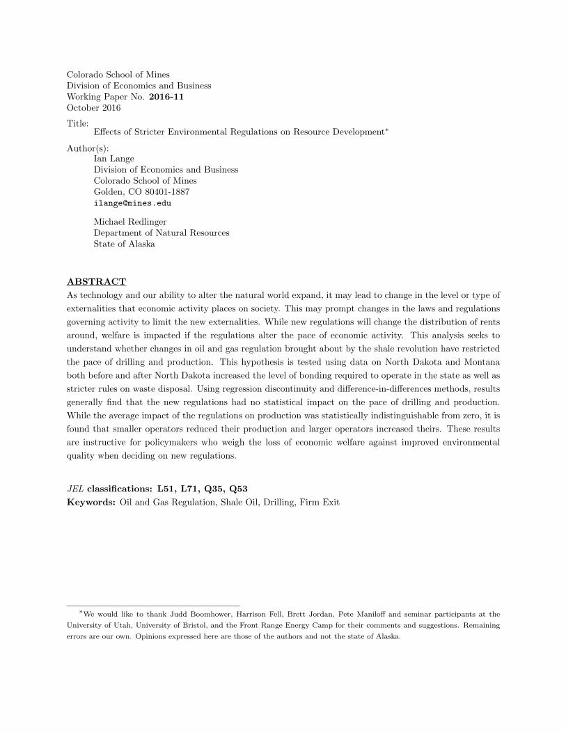
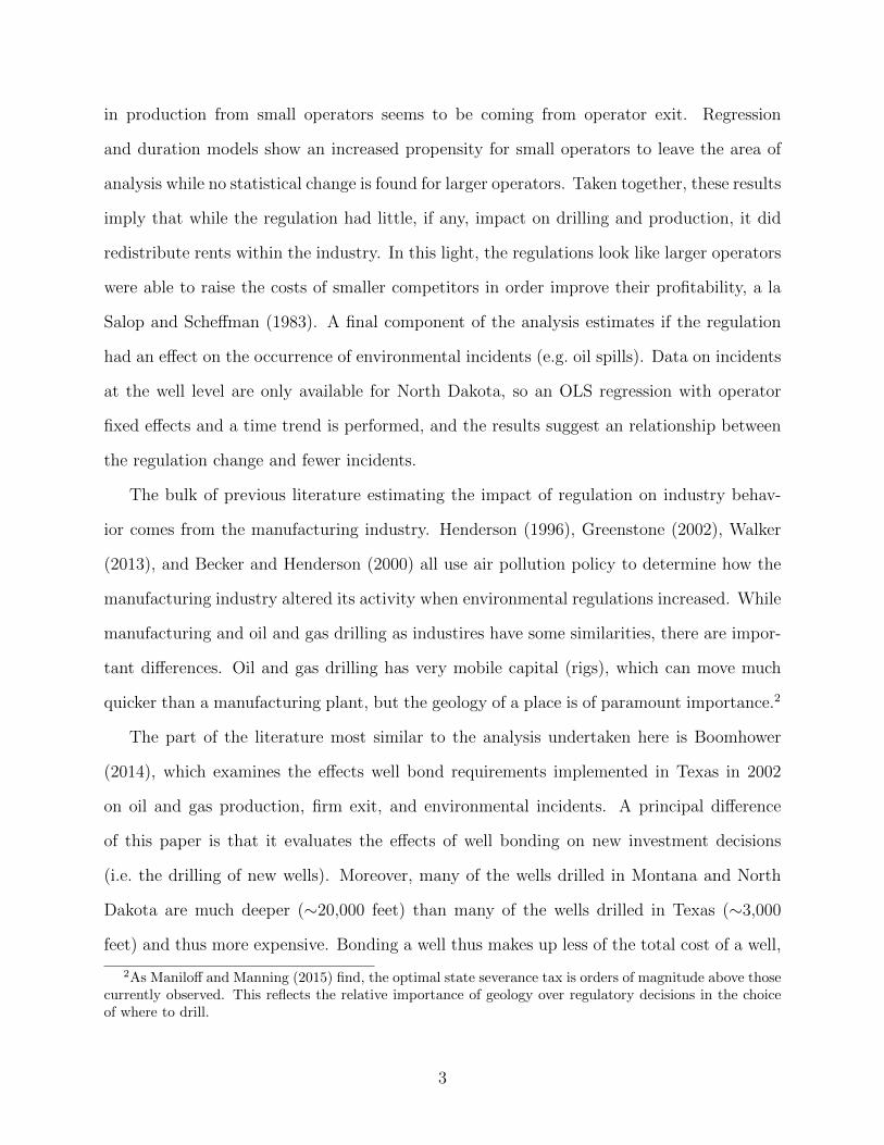
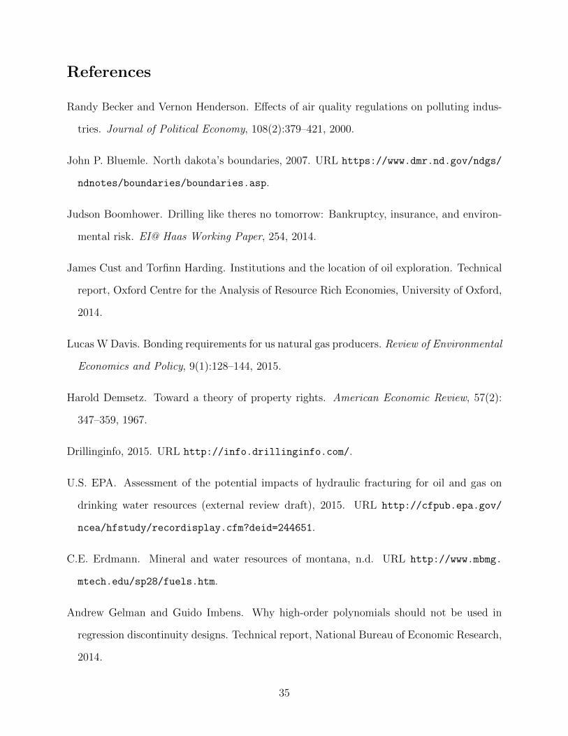
Figure 1 presents a histogram of wells drilled within fifty miles of the MT-ND border
in the 2 years leading up the regulation revisions (April 2010–March 2012). There is no
obvious discontinuity in the density of drilling activity at the border before the regulation
change. This figure also shows that drilling becomes more prevalent in North Dakota as
distance from the border increases. This is largely explained by the existence of a fold in
the subsurface rock formations called the “Nesson Anticline” that creates a so called “sweet
spot” because natural fractures in the rock enhance oil production. The flexible functional
9
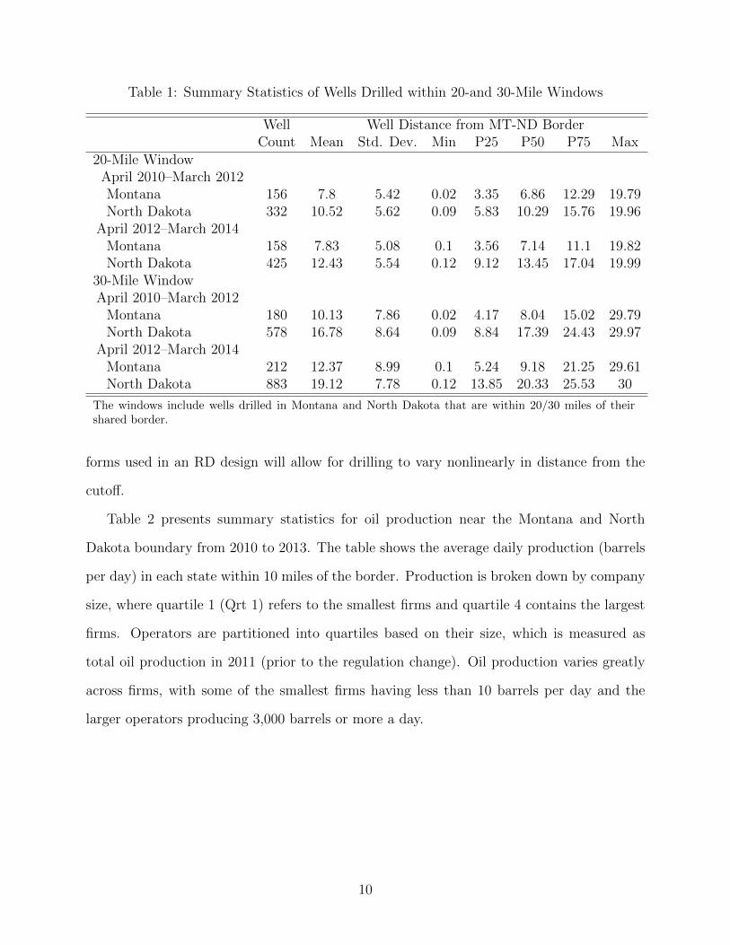
Table 1: Summary Statistics of Wells Drilled within 20-and 30-Mile Windows
Well Well Distance from MT-ND BorderCount Mean Std. Dev. Min P25 P50 P75 Max
20-Mile WindowApril 2010–March 2012Montana 156 7.8 5.42 0.02 3.35 6.86 12.29 19.79North Dakota 332 10.52 5.62 0.09 5.83 10.29 15.76 19.96
April 2012–March 2014Montana 158 7.83 5.08 0.1 3.56 7.14 11.1 19.82North Dakota 425 12.43 5.54 0.12 9.12 13.45 17.04 19.99
30-Mile WindowApril 2010–March 2012
Montana 180 10.13 7.86 0.02 4.17 8.04 15.02 29.79North Dakota 578 16.78 8.64 0.09 8.84 17.39 24.43 29.97
April 2012–March 2014Montana 212 12.37 8.99 0.1 5.24 9.18 21.25 29.61North Dakota 883 19.12 7.78 0.12 13.85 20.33 25.53 30
The windows include wells drilled in Montana and North Dakota that are within 20/30 miles of theirshared border.
forms used in an RD design will allow for drilling to vary nonlinearly in distance from the
cutoff.
Table 2 presents summary statistics for oil production near the Montana and North
Dakota boundary from 2010 to 2013. The table shows the average daily production (barrels
per day) in each state within 10 miles of the border. Production is broken down by company
size, where quartile 1 (Qrt 1) refers to the smallest firms and quartile 4 contains the largest
firms. Operators are partitioned into quartiles based on their size, which is measured as
total oil production in 2011 (prior to the regulation change). Oil production varies greatly
across firms, with some of the smallest firms having less than 10 barrels per day and the
larger operators producing 3,000 barrels or more a day.
10
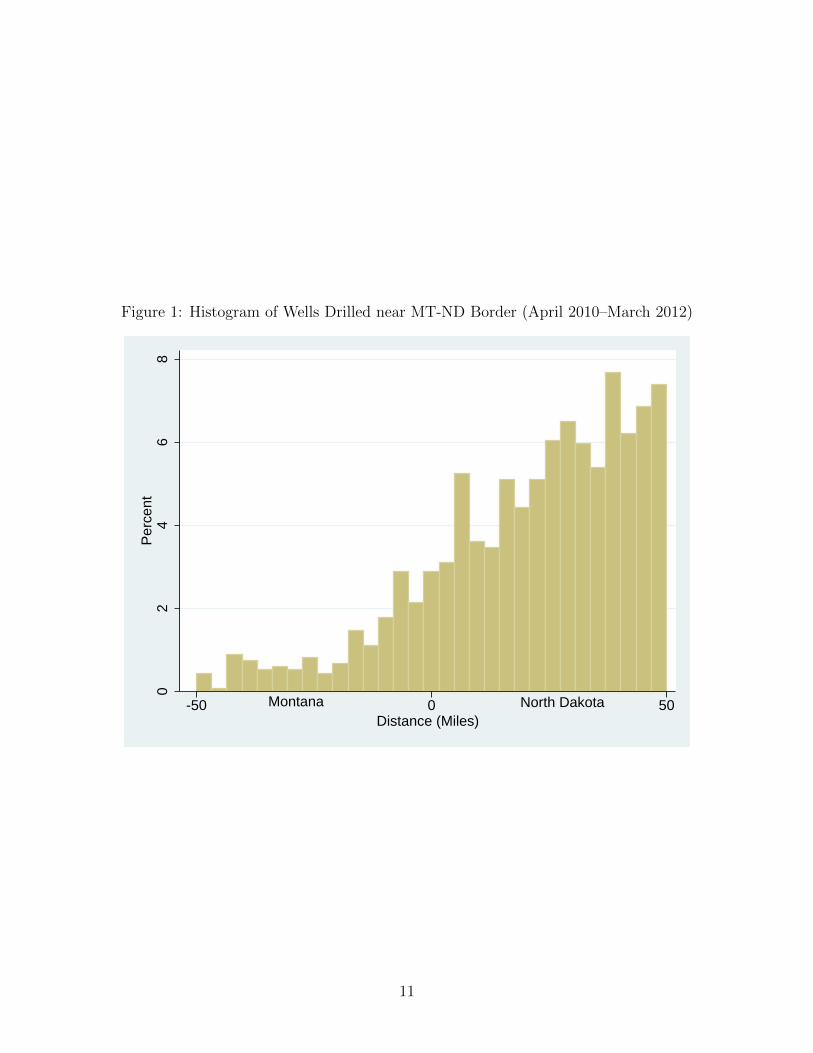
Figure 1: Histogram of Wells Drilled near MT-ND Border (April 2010–March 2012)
02
46
8P
erce
nt
-50 0 50Distance (Miles)
North DakotaMontana
11
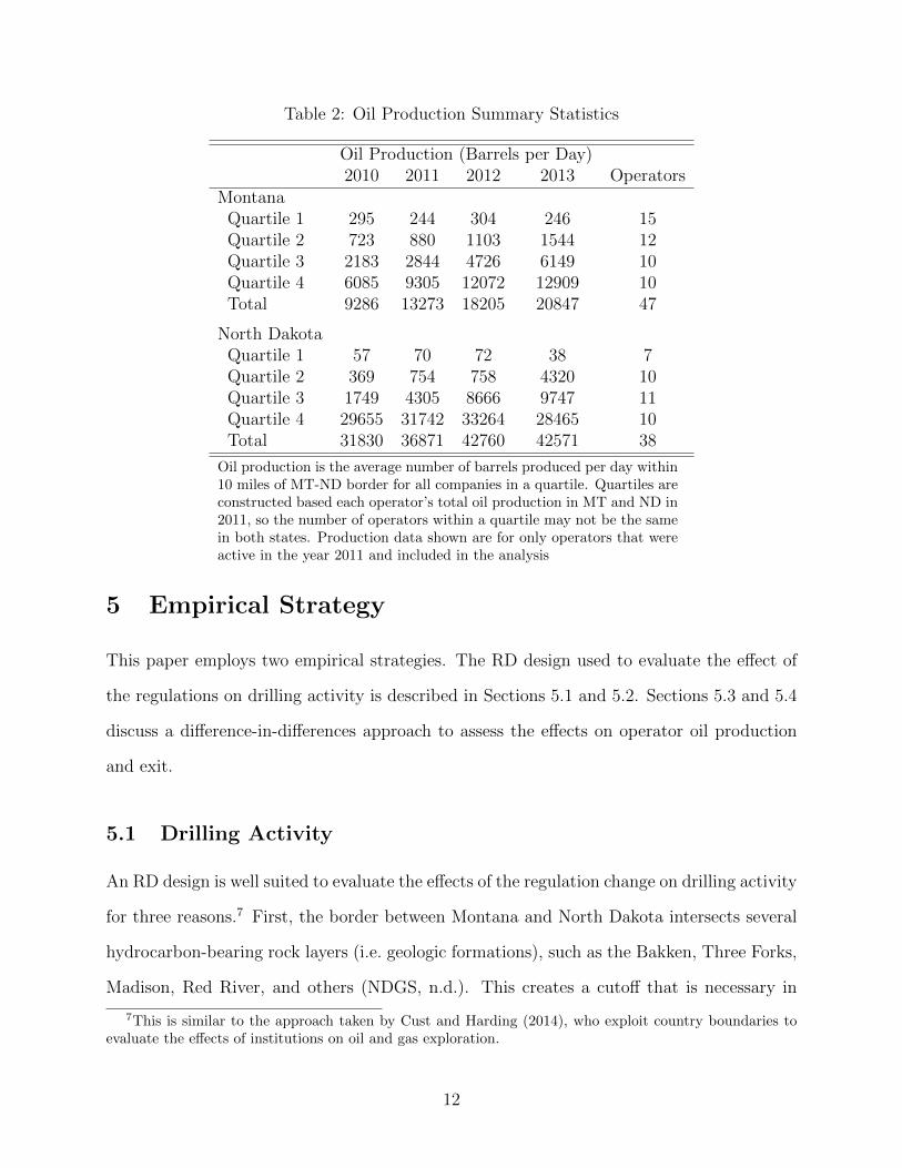
Table 2: Oil Production Summary Statistics
Oil Production (Barrels per Day)2010 2011 2012 2013 Operators
MontanaQuartile 1 295 244 304 246 15Quartile 2 723 880 1103 1544 12Quartile 3 2183 2844 4726 6149 10Quartile 4 6085 9305 12072 12909 10Total 9286 13273 18205 20847 47
North DakotaQuartile 1 57 70 72 38 7Quartile 2 369 754 758 4320 10Quartile 3 1749 4305 8666 9747 11Quartile 4 29655 31742 33264 28465 10Total 31830 36871 42760 42571 38
Oil production is the average number of barrels produced per day within10 miles of MT-ND border for all companies in a quartile. Quartiles areconstructed based each operator’s total oil production in MT and ND in2011, so the number of operators within a quartile may not be the samein both states. Production data shown are for only operators that wereactive in the year 2011 and included in the analysis
5 Empirical Strategy
This paper employs two empirical strategies. The RD design used to evaluate the effect of
the regulations on drilling activity is described in Sections 5.1 and 5.2. Sections 5.3 and 5.4
discuss a difference-in-differences approach to assess the effects on operator oil production
and exit.
5.1 Drilling Activity
An RD design is well suited to evaluate the effects of the regulation change on drilling activity
for three reasons.7 First, the border between Montana and North Dakota intersects several
hydrocarbon-bearing rock layers (i.e. geologic formations), such as the Bakken, Three Forks,
Madison, Red River, and others (NDGS, n.d.). This creates a cutoff that is necessary in
7This is similar to the approach taken by Cust and Harding (2014), who exploit country boundaries toevaluate the effects of institutions on oil and gas exploration.
12
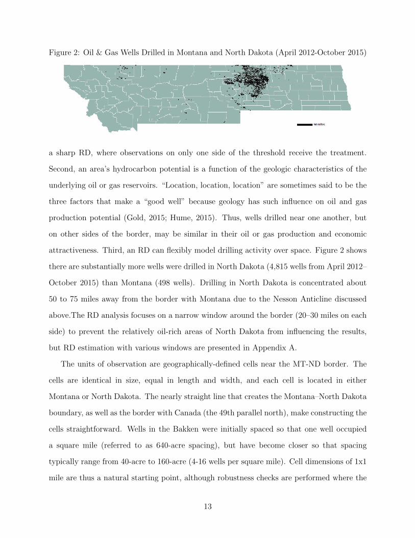
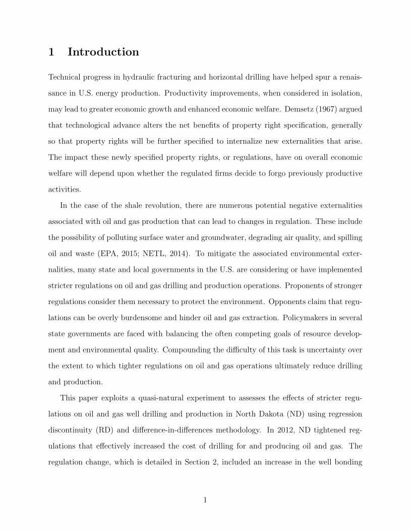
Figure 2: Oil & Gas Wells Drilled in Montana and North Dakota (April 2012-October 2015)
a sharp RD, where observations on only one side of the threshold receive the treatment.
Second, an area’s hydrocarbon potential is a function of the geologic characteristics of the
underlying oil or gas reservoirs. “Location, location, location” are sometimes said to be the
three factors that make a “good well” because geology has such influence on oil and gas
production potential (Gold, 2015; Hume, 2015). Thus, wells drilled near one another, but
on other sides of the border, may be similar in their oil or gas production and economic
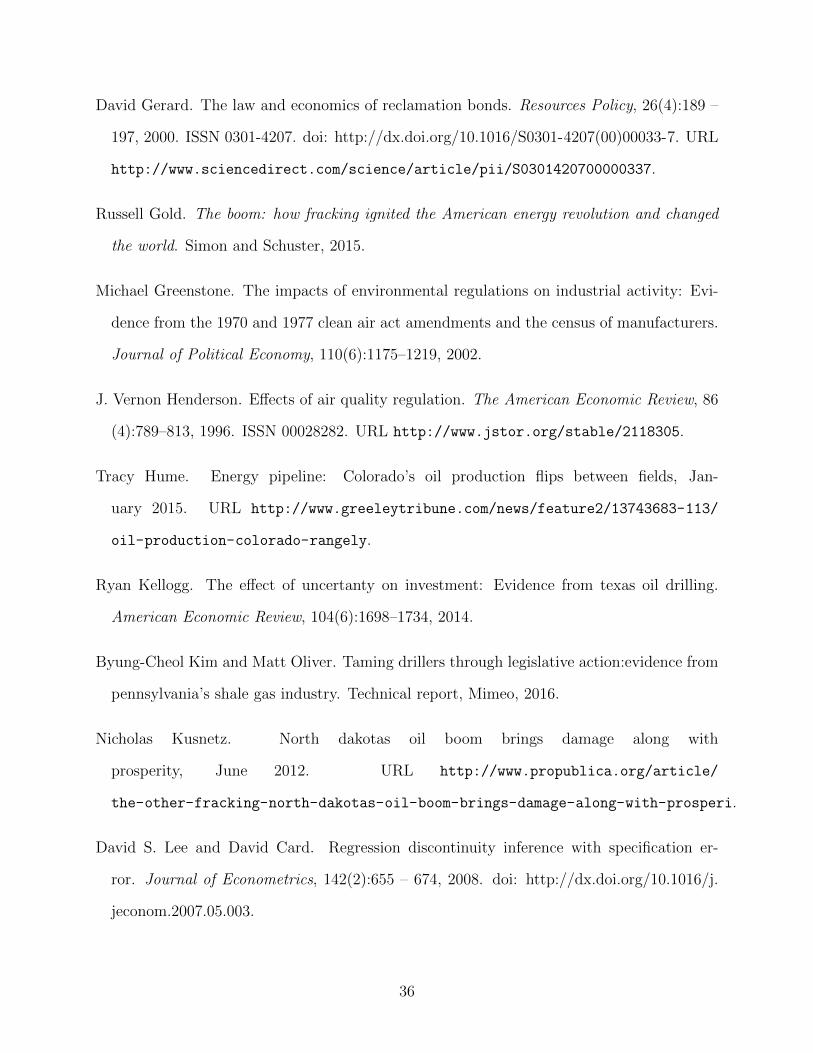
attractiveness. Third, an RD can flexibly model drilling activity over space. Figure 2 shows
there are substantially more wells were drilled in North Dakota (4,815 wells from April 2012–
October 2015) than Montana (498 wells). Drilling in North Dakota is concentrated about
50 to 75 miles away from the border with Montana due to the Nesson Anticline discussed
above.The RD analysis focuses on a narrow window around the border (20–30 miles on each
side) to prevent the relatively oil-rich areas of North Dakota from influencing the results,
but RD estimation with various windows are presented in Appendix A.
The units of observation are geographically-defined cells near the MT-ND border. The
cells are identical in size, equal in length and width, and each cell is located in either
Montana or North Dakota. The nearly straight line that creates the Montana–North Dakota
boundary, as well as the border with Canada (the 49th parallel north), make constructing the
cells straightforward. Wells in the Bakken were initially spaced so that one well occupied
a square mile (referred to as 640-acre spacing), but have become closer so that spacing
typically range from 40-acre to 160-acre (4-16 wells per square mile). Cell dimensions of 1x1
mile are thus a natural starting point, although robustness checks are performed where the
13
cell dimensions are modified to 5x5 miles.
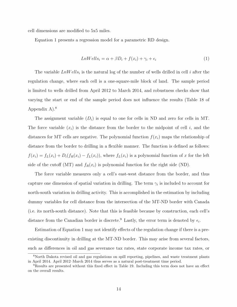
Equation 1 presents a regression model for a parametric RD design.
LnWellsi = α + βDi + f(xi) + γi + εi (1)
The variable LnWellsi is the natural log of the number of wells drilled in cell i after the
regulation change, where each cell is a one-square-mile block of land. The sample period
is limited to wells drilled from April 2012 to March 2014, and robustness checks show that
varying the start or end of the sample period does not influence the results (Table 18 of
Appendix A).8
The assignment variable (Di) is equal to one for cells in ND and zero for cells in MT.
The force variable (xi) is the distance from the border to the midpoint of cell i, and the
distances for MT cells are negative. The polynomial function f(xi) maps the relationship of
distance from the border to drilling in a flexible manner. The function is defined as follows:
f(xi) = fL(xi) +Di(fR(xi)− fL(xi)), where fL(xi) is a polynomial function of x for the left
side of the cutoff (MT) and fR(xi) is polynomial function for the right side (ND).
The force variable measures only a cell’s east-west distance from the border, and thus
capture one dimension of spatial variation in drilling. The term γi is included to account for
north-south variation in drilling activity. This is accomplished in the estimation by including
dummy variables for cell distance from the intersection of the MT-ND border with Canada
(i.e. its north-south distance). Note that this is feasible because by construction, each cell’s
distance from the Canadian border is discrete.9 Lastly, the error term is denoted by εi.
Estimation of Equation 1 may not identify effects of the regulation change if there is a pre-
existing discontinuity in drilling at the MT-ND border. This may arise from several factors,
such as differences in oil and gas severance tax rates, state corporate income tax rates, or
8North Dakota revised oil and gas regulations on spill reporting, pipelines, and waste treatment plantsin April 2014. April 2012–March 2014 thus serves as a natural post-treatment time period.
9Results are presented without this fixed effect in Table 19. Including this term does not have an effecton the overall results.
14
other regulatory requirements. Hence it is necessary to estimate the how the discontinuity
at the border changes following the stricter regulations.
In equation 2, the pre-and post-treatment sample periods are pooled to estimate the
difference in the discontinuity before and after the revision to the regulations. This is similar
to the “pretest RD” method introduced by Wing and Cook (2013) (See Appendix B). The
pretest RD improves identification of the standard RD design by including pre-treatment
observations, which contain information on the underlying relationship between the force
variable and outcome variable. In this paper, not only do pre-treatment observations help
establish the relationship between distance from the border and drilling activity, but they
are also necessary to account for a potential pre-existing discontinuity at the border.
LnWellsit = ρDit + ζSi + h0(xi) + Tit(h1(xi)− h0(xi)) + γi + εit (2)
where h0(xi) = h0L(xi) + Si(h0R(xi)− h0L(xi)),
and h1(xi) = h1L(xi) + Si(h1R(xi)− h1L(xi))
The dependent variable (LnWellsit) is the natural log of the number of wells drilled
in cell i in period t. There are two periods: t = 0 is the pre-treatment period (April
2010–March 2012) and t = 1 is the post-treatment period (April 2012–March 2014). Note
that Tables 17 and 18 of Appendix A show that varying the sample period does not alter
conclusions drawn from the results. The variable Si indicates whether the cell is in North
Dakota (Si = 1) or Montana (Si = 0). The polynomial functions allow drilling activity to
vary across time periods (pre-and post-treatment) and the cutoff. The functions h0(xi) and
h1(xi) are polynomials for the pre-treatment and post-treatment periods, respectively. The
variable Tt is equal to zero for cells in the pre-treatment (T0 = 0) period and equal one for
cells in the post-treatment (T1 = 1) period. For example, for t = 0, drilling activity follows
the polynomial h0(xi), which in turn differs for the Montana side (h0L(xi)) and North Dakota
side (h0R(xi)). The term γi is the fixed effect for the north-south position of cell i, and εit is
the error term.
15
A parametric RD is applied, as opposed to a nonparametric RD, because the force variable
is discrete. Distance is measured from the border to the midpoint of each cell (0.5, 1.5, 2.5
miles, etc.). Lee and Card (2008) note that the non-parametric and semi-parametric RD
methods rely on comparing outcomes in arbitrary small neighborhoods around the threshold.
In cases with discrete force variables, it is not possible to be arbitrarily close the threshold
even as the sample size grows. The approach recommended by Lee and Card (2008), which
is followed in this analysis, is to use parametric functional form and cluster the standard
errors on the force variable. Non-parametric RD yields similar results though (Table 16 of
Appendix A).
The polynomial order is selected based on the specification’s Akaike information criterion
(AIC) value. Based on the findings by Gelman and Imbens (2014), who caution against using
high order polynomials, only models with zero through second-order polynomials are consid-
ered. In choosing the width of the window around the border, there is a trade-off between
observations and potential bias. Results for 20-mile and 30-mile windows are presented in
Section 6, but results for additional windows in Appendix A give similar findings.
5.2 RD Design Identification
This section discusses five issues that threaten identification through the RD design. First,
a necessary assumption is that the conditional regression functions are continuous at the
cutoff. That is, there is no discontinuity in the outcome variable at the cutoff— that is
unrelated to the treatment. As discussed in Section 5.1, this assumption may be violated
because of pre-existing differences between Montana and North Dakota. This is resolved by
pooling pre-treatment and post-treatment data into a single RD (Equation 2) and estimating
the difference in this discontinuity following the regulation revisions.
The second identification issue is whether there is a discontinuity in the density of the
force variable near the cutoff. In this paper, the unit of observation is a geographically-
defined cell, and firm decisions on where to drill are the outcomes of interest. Thus, if
16
drilling is relatively sparse on the North Dakota side following the regulation change, this
would not necessarily imply that the identification strategy is invalid but rather that the
new regulations has an effect. Figure 3 in Section 3 shows there is no apparent discontinuity
in the density of drilling activity at the boundary (i.e. firms don’t avoid the places near the
border) in the two years leading up to the regulation change (April 2010–March 2012).
Third, identifying the treatment effect requires the stable unit treatment value assump-
tion (SUTVA) to hold. The Montana observations must not be affected by the treatment
applied to North Dakota. This assumption is violated if stricter regulations in North Dakota
cause firms to relocate to Montana, which would cause drilling activity in Montana to be
higher than it would be otherwise. Since the validity of this assumption is unknown here,
we consider the estimation results to be an upper bound of the average treatment effect at
the threshold.
Fourth, the enactment of regulation revisions may coincide with temporal shifts in drilling
from one state to the other. A possible scenario is that drilling was concentrated in one state
in the years leading up to the regulation change; that state became saturated with wells near
the time of regulation change, and activity then shifted to other state. Such a situation may
give the incorrectly attribute shift in drilling to the regulations. To deal with this issue, a
control variable for the number of previously wells drilled within a cell is added to equation 1.
The number of wells previously drilled is specified in both linear and quadratic forms, which
allows for drilling within a cell to become saturated and decline over time There is no
meaningful difference in the estimation results (Table 21 of Appendix A) when including
this control.
Fifth and finally, a common identification issue with applications of RD is endogeneity
of the cutoff’s placement. It is highly unlikely that oil and gas deposits had any influence
over location of the Montana-North Dakota border, and furthermore that such placement
would be correlated with the 2012 regulation change. The current Montana-North Dakota
border was originally the eastern border of the Idaho territory created by Congress in 1863
17
(State Historical Society of North Dakota, 2016). This later become the border between
Montana and North Dakota, when the two states where formed in 1889. The first oil wells
were drilled in Montana and North Dakota in 1901 and 1929, respectively (Erdmann, n.d.;
NDGS, n.d.). Moreover, the border is reported to have been chosen “out of the blue”, and
“The line does not coincide with any particular section or half-section line, or anything else
of local or regional significance.” (Bluemle, 2007).
5.3 Oil Production and Exit
A difference-in-difference approach is used to determine the effects of the more stringent
regulations on operator oil production and exit. Higher bond requirements may increase the
marginal cost of oil production and cause firms to reduce output. For example, operators
could shut in wells that are no longer profitable or drill fewer wells, which would subsequently
decrease production. The stricter drilling waste disposal rules are not expected to affect
production at existing wells, but these rules can reduce production by discouraging the
drilling of new wells.
Equation 3 estimates the effects of the revised regulations on operator-level oil production.
LnProdijt = τDjt + θi + κj + λt + ηijt (3)
The dependent variable (LnProdijt) is the natural log of oil produced by operator i in
state j during month t. The quantities of oil produced are limited to an operator’s production
from wells within 10 miles of the MT-ND boundary, which ensures the treatment and control
groups are similar. The treatment variable (Djt) is equal to one for observations in North
Dakota after the regulation change (April 2012 and onward) and zero otherwise. Time-
invariant unobservables are controlled for with fixed effects for the operator (θi), state (κj)
and month (λt). The last term (ηijt) is the idiosyncratic error.
The final regression model is shown in Equation 4, which estimates the effect on operator
18
exit from the 10-mile window in North Dakota.10 In the estimation of Equation 3, oper-
ators that shut down production completely leave the sample and are no longer observed,
which creates an attrition bias. This could underestimate the effects of the regulation on oil
production if some firms shut down production or sell off wells and exit.
Exitijt = µDjt + φi + ψj + ωt + υijt (4)
The dependent variable (Exitijt) is equal to one if operator i exits the study area of State
j in month t; and zero otherwise. Note that this measures only if an operator exits the
area within the 10 miles of the border and not whether it ceases operations in the entire
state. An exit occurs in the month in which an operator’s production falls to zero and
remains shutdown throughout the sample period. The treatment variable (Djt) is equal to
one for observations in North Dakota after the regulation change (April 2012 and onward)
and zero otherwise. Fixed effects are included to account for time-invariant effects specific
to the operator (φi), state (ψj), and month of production (ωt). The last term, υijt, is the
idiosyncratic error.
Equations 3 and 4 estimate the average effect across all operators, but firms may respond
differently depending on their size. Section 6.2 provides estimation results where the coeffi-
cient estimate for the treatment variable is allowed differ by firm size. Each operator’s total
oil production in all of Montana and North Dakota in 2011 (prior to the regulation change)
is the proxy used for firm size.
It is usually more costly for smaller firms to meet well bond requirements. Operators,
especially small companies, often post a surety bond. As discussed in Section 2, in this
situation, a surety company issues a bond to the operator, who then submits the bond to
the state regulator. The operator pays the surety company a premium, which is typically a
percentage of the face value of the bond. Firms with relatively limited assets, with poor envi-
ronmental or safety records, or in precarious financial positions, often pay higher premiums.
10A duration analysis performed in Appendix C provides similar findings.
19
Smaller firms may pay higher premiums to surety companies because these operators are po-
tentially judgment proof, which occurs when a firm is unable to pay its full legal liabilities.
For example, in bankruptcy, a company is liable up to only the value of its assets and can
have the obligations that exceed this amount dissolved. Bonding requirements could require
operators to invest in safety and set output at levels that are socially optimal if operator
behavior was perfectly observable by surety companies. Surety companies recognize that
because operator behavior is not perfectly observable, smaller firms have less of an incentive
to undertake safety measures and avoid risk because they will not be fully liable for poten-
tial damages. Thus, these operators face higher premiums, and increasing the well bonding
requirement has a larger financial impact on smaller (and potentially judgment proof) firms
than larger firms.
5.4 Difference-in-Difference Identification
There are three primary identification issues to address with the estimation equations 3 and
4. First, there is the potential for policy endogeneity. That is, there may be unobserved
factors that influence production (or firm exit) and North Dakota’s adoption of the revised
regulations. Inclusion of the state fixed effect controls for time-invariant unobservables spe-
cific to each state. These unobservables may be differences across the two states in existing
tax structures, general friendliness to resource development, geographic features within the
window. Time-varying, state-level unobservables, however, are not accounted for with a state
fixed effect. One potential time-varying factor is the Bakken Shale Play boom that began
in 2008. The breakthroughs in horizontal drilling and hydraulic fracturing may have had
different effects on oil activity in Montana and North Dakota. North Dakota encompasses
more of the Bakken and the so called “sweet spots” that offer higher oil production rates.
As the Bakken boom was occurring, it is conceivable that policy-makers in North Dakota
judged that passing stricter regulations would have a limited effect on oil activity because
evolving technology would unlock the state’s rich hydrocarbon potential. To deal with this
20
issue, the sample is restricted to oil production in each state that is within 10 miles of the
MT-ND border. This ensures that the resource potential is very similar across the treatment
and control groups and the regulation change should not be endogenous in the models.
The second identification issue is the appropriateness of the control group. To accurately
estimate the treatment effect, the control group must serve as an appropriate counterfactual
to North Dakota. Including oil production from only wells within a 10-mile window on each
side of the border allows for wells in the sample to share similar geology and production
potential. Figure 3 depicts Montana and North Dakota oil production within the 10-mile
window and shows that pre-treatment, production in the two states generally moves in step.
Formal tests show no difference in pre-treatment trends between the two states (Table 6).
Third and finally, as discussed in Section 5.2, the SUTVA is required to identify the
average treatment effect. The control group may be contaminated if firms shift production
activities to Montana in response to the regulation change. This is an issue in many studies
that attempt to estimate the effects of environmental regulations on firm investment decisions
(Millimet et al., 2009). Thus, as in the RD design, the difference-in-difference estimation
results can be interpreted as an upper bound of the treatment effect.
6 Results
6.1 RD Results
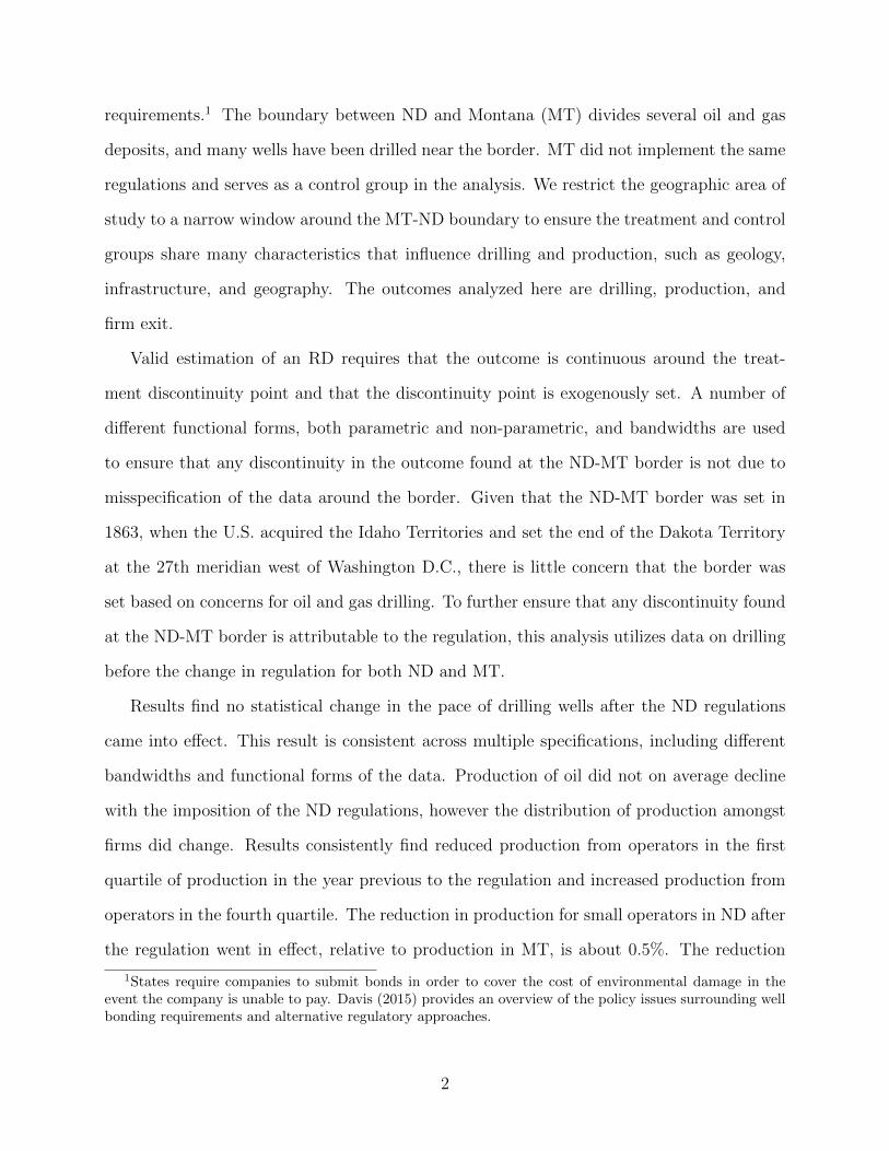
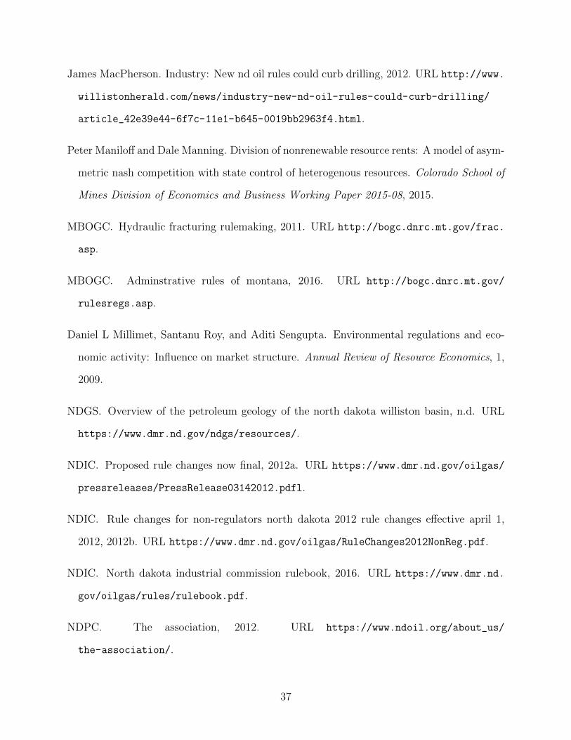
Figure 3 shows well drilling near the MT-ND border in the two-year period prior to the
regulation change (April 2010–March 2012). The log number of wells drilled within a cell is
on the vertical axis, and the cell’s distance from the border is shown on the horizontal axis.
The cutoff is at distance zero with Montana on the left side and North Dakota to the right.
The left panel of Figure 3 captures a 20-mile window on each side the border with a fitted
quadratic. Estimation of equation 1 with the function f(xi) as a second-order polynomial
yields the lowest AIC score for all models with zero to second-degree polynomials. The right
21
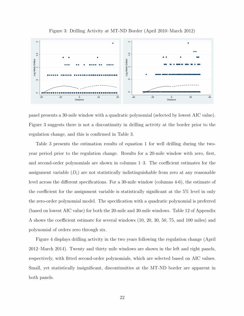
Figure 3: Drilling Activity at MT-ND Border (April 2010–March 2012)0
.51
1.5
2Lo
g W
ells
Dril
led
-20 -10 0 10 20Distance
0.5
11.
52
Log
Wel
ls D
rille
d
-40 -20 0 20 40Distance
panel presents a 30-mile window with a quadratic polynomial (selected by lowest AIC value).
Figure 3 suggests there is not a discontinuity in drilling activity at the border prior to the
regulation change, and this is confirmed in Table 3.
Table 3 presents the estimation results of equation 1 for well drilling during the two-
year period prior to the regulation change. Results for a 20-mile window with zero, first,
and second-order polynomials are shown in columns 1–3. The coefficient estimates for the
assignment variable (Di) are not statistically indistinguishable from zero at any reasonable
level across the different specifications. For a 30-mile window (columns 4-6), the estimate of
the coefficient for the assignment variable is statistically significant at the 5% level in only
the zero-order polynomial model. The specification with a quadratic polynomial is preferred
(based on lowest AIC value) for both the 20-mile and 30-mile windows. Table 12 of Appendix
A shows the coefficient estimate for several windows (10, 20, 30, 50, 75, and 100 miles) and
polynomial of orders zero through six.
Figure 4 displays drilling activity in the two years following the regulation change (April
2012–March 2014). Twenty and thirty mile windows are shown in the left and right panels,
respectively, with fitted second-order polynomials, which are selected based on AIC values.
Small, yet statistically insignificant, discontinuities at the MT-ND border are apparent in
both panels.
22
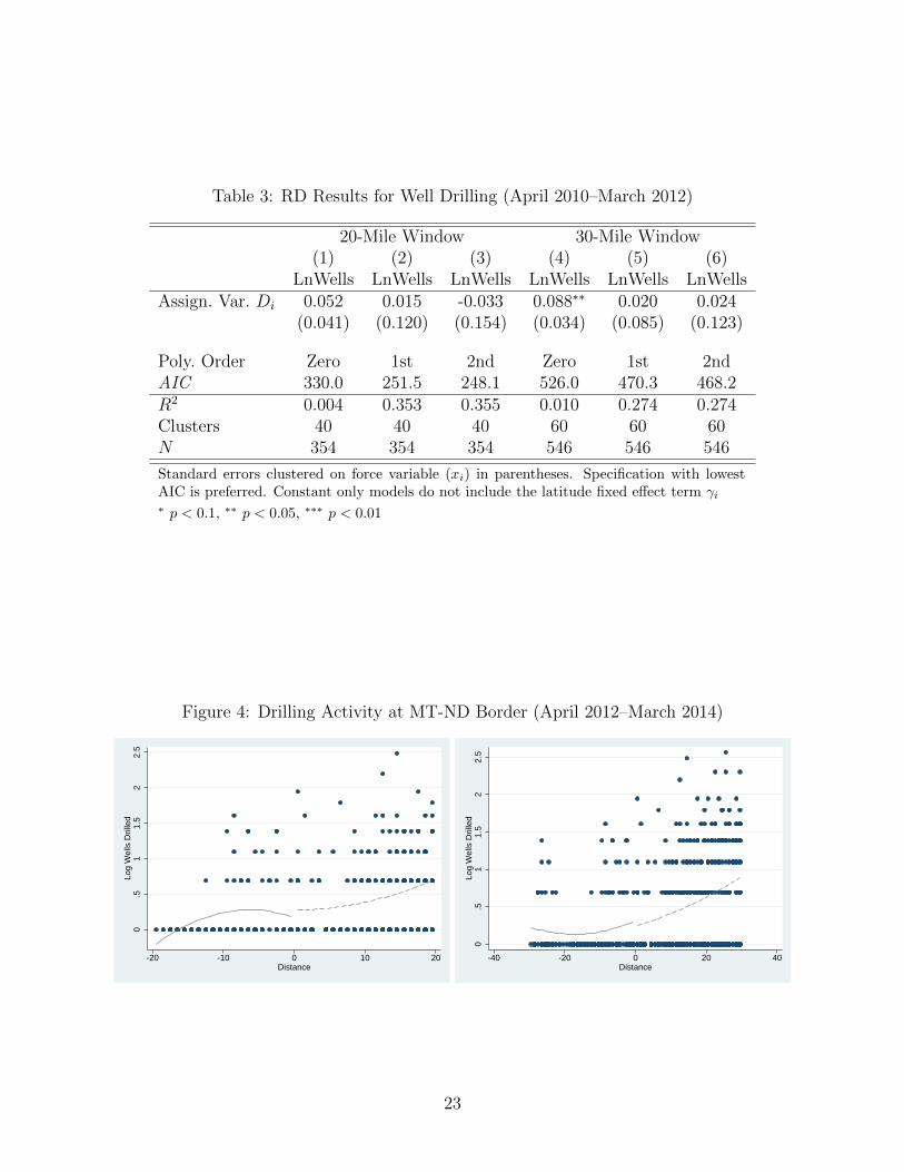
Table 3: RD Results for Well Drilling (April 2010–March 2012)
20-Mile Window 30-Mile Window(1) (2) (3) (4) (5) (6)
LnWells LnWells LnWells LnWells LnWells LnWellsAssign. Var. Di 0.052 0.015 -0.033 0.088∗∗ 0.020 0.024
(0.041) (0.120) (0.154) (0.034) (0.085) (0.123)
Poly. Order Zero 1st 2nd Zero 1st 2ndAIC 330.0 251.5 248.1 526.0 470.3 468.2R2 0.004 0.353 0.355 0.010 0.274 0.274Clusters 40 40 40 60 60 60N 354 354 354 546 546 546
Standard errors clustered on force variable (xi) in parentheses. Specification with lowestAIC is preferred. Constant only models do not include the latitude fixed effect term γi∗ p < 0.1, ∗∗ p < 0.05, ∗∗∗ p < 0.01
Figure 4: Drilling Activity at MT-ND Border (April 2012–March 2014)
0.5
11.
52
2.5
Log
Wel
ls D
rille
d
-20 -10 0 10 20Distance
0.5
11.
52
2.5
Log
Wel
ls D
rille
d
-40 -20 0 20 40Distance
23
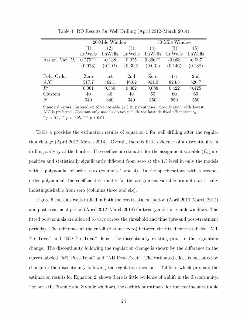
Table 4: RD Results for Well Drilling (April 2012–March 2014)
20-Mile Window 30-Mile Window(1) (2) (3) (4) (5) (6)
LnWells LnWells LnWells LnWells LnWells LnWellsAssign. Var. Di 0.275∗∗∗ -0.138 0.025 0.396∗∗∗ -0.063 -0.097
(0.073) (0.202) (0.309) (0.061) (0.146) (0.238)
Poly. Order Zero 1st 2nd Zero 1st 2ndAIC 517.7 462.1 460.2 961.0 823.8 820.7R2 0.061 0.359 0.362 0.088 0.422 0.425Clusters 40 40 40 60 60 60N 340 340 340 550 550 550
Standard errors clustered on force variable (xi) in parentheses. Specification with lowestAIC is preferred. Constant only models do not include the latitude fixed effect term γi∗ p < 0.1, ∗∗ p < 0.05, ∗∗∗ p < 0.01
Table 4 provides the estimation results of equation 1 for well drilling after the regula-
tion change (April 2012–March 2014). Overall, there is little evidence of a discontinuity in
drilling activity at the border. The coefficient estimates for the assignment variable (Di) are
positive and statistically significantly different from zero at the 1% level in only the models
with a polynomial of order zero (columns 1 and 4). In the specifications with a second-
order polynomial, the coefficient estimates for the assignment variable are not statistically
indistinguishable from zero (columns three and six).
Figure 5 contains wells drilled in both the pre-treatment period (April 2010–March 2012)
and post-treatment period (April 2012–March 2014) for twenty and thirty mile windows. The
fitted polynomials are allowed to vary across the threshold and time (pre-and post-treatment
periods). The difference at the cutoff (distance zero) between the fitted curves labeled “MT
Pre-Treat” and “ND Pre-Treat” depict the discontinuity existing prior to the regulation
change. The discontinuity following the regulation change is shown by the difference in the
curves labeled “MT Post-Treat” and “ND Post-Treat”. The estimated effect is measured by
change in the discontinuity following the regulation revisions. Table 5, which presents the
estimation results for Equation 2, shows there is little evidence of a shift in the discontinuity.
For both the 20-mile and 30-mile windows, the coefficient estimate for the treatment variable
24
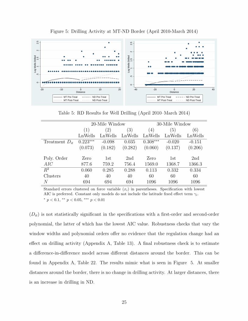
Figure 5: Drilling Activity at MT-ND Border (April 2010-March 2014)0
.51
1.5
22.
5Lo
g W
ells
Dril
led
-20 -10 0 10 20Distance
MT Pre-Treat ND Pre-TreatMT Post-Treat ND Post-Treat
0.5
11.
52
2.5
Log
Wel
ls D
rille
d
-40 -20 0 20 40Distance
MT Pre-Treat ND Pre-TreatMT Post-Treat ND Post-Treat
Table 5: RD Results for Well Drilling (April 2010–March 2014)
20-Mile Window 30-Mile Window(1) (2) (3) (4) (5) (6)
LnWells LnWells LnWells LnWells LnWells LnWellsTreatment Dit 0.223∗∗∗ -0.098 0.035 0.308∗∗∗ -0.020 -0.151
(0.073) (0.182) (0.282) (0.060) (0.137) (0.206)
Poly. Order Zero 1st 2nd Zero 1st 2ndAIC 877.6 759.2 756.4 1569.0 1368.7 1366.3R2 0.060 0.285 0.288 0.113 0.332 0.334Clusters 40 40 40 60 60 60N 694 694 694 1096 1096 1096
Standard errors clustered on force variable (xi) in parentheses. Specification with lowestAIC is preferred. Constant only models do not include the latitude fixed effect term γi.∗ p < 0.1, ∗∗ p < 0.05, ∗∗∗ p < 0.01
(Dit) is not statistically significant in the specifications with a first-order and second-order
polynomial, the latter of which has the lowest AIC value. Robustness checks that vary the
window widths and polynomial orders offer no evidence that the regulation change had an
effect on drilling activity (Appendix A, Table 13). A final robustness check is to estimate
a difference-in-difference model across different distances around the border. This can be
found in Appendix A, Table 22. The results mimic what is seen in Figure 5. At smaller
distances around the border, there is no change in drilling activity. At larger distances, there
is an increase in drilling in ND.
25
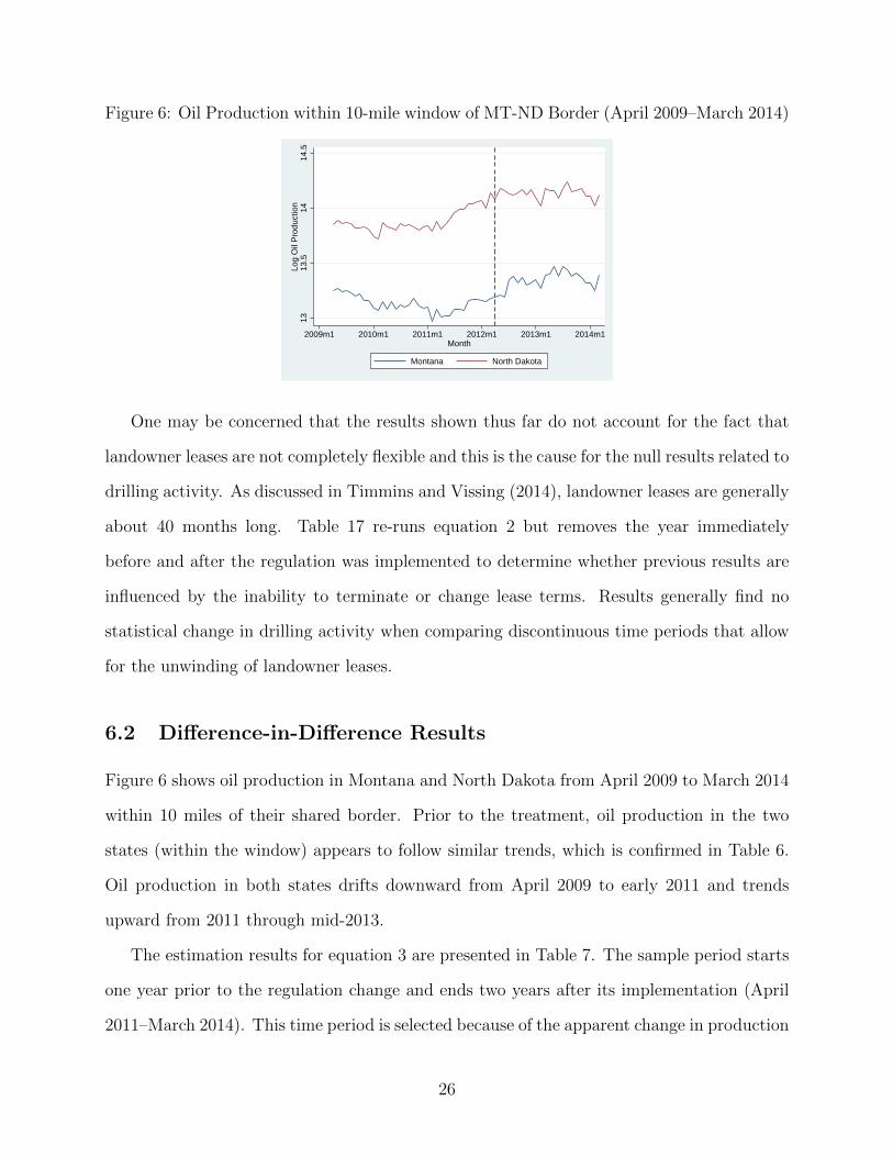
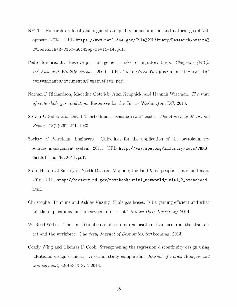
Figure 6: Oil Production within 10-mile window of MT-ND Border (April 2009–March 2014)
1313
.514
14.5
Log
Oil
Pro
duct
ion
2009m1 2010m1 2011m1 2012m1 2013m1 2014m1Month
Montana North Dakota
One may be concerned that the results shown thus far do not account for the fact that
landowner leases are not completely flexible and this is the cause for the null results related to
drilling activity. As discussed in Timmins and Vissing (2014), landowner leases are generally
about 40 months long. Table 17 re-runs equation 2 but removes the year immediately
before and after the regulation was implemented to determine whether previous results are
influenced by the inability to terminate or change lease terms. Results generally find no
statistical change in drilling activity when comparing discontinuous time periods that allow
for the unwinding of landowner leases.
6.2 Difference-in-Difference Results
Figure 6 shows oil production in Montana and North Dakota from April 2009 to March 2014
within 10 miles of their shared border. Prior to the treatment, oil production in the two
states (within the window) appears to follow similar trends, which is confirmed in Table 6.
Oil production in both states drifts downward from April 2009 to early 2011 and trends
upward from 2011 through mid-2013.
The estimation results for equation 3 are presented in Table 7. The sample period starts
one year prior to the regulation change and ends two years after its implementation (April
2011–March 2014). This time period is selected because of the apparent change in production
26
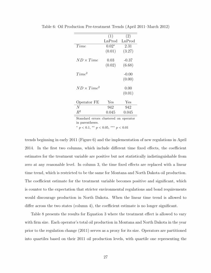
Table 6: Oil Production Pre-treatment Trends (April 2011–March 2012)
(1) (2)LnProd LnProd
Time 0.02∗ 2.31(0.01) (3.27)
ND × Time 0.03 -0.37(0.02) (6.68)
Time2 -0.00(0.00)
ND × Time2 0.00(0.01)
Operator FE Yes YesN 942 942R2 0.045 0.045
Standard errors clustered on operatorin parentheses.∗ p < 0.1, ∗∗ p < 0.05, ∗∗∗ p < 0.01
trends beginning in early 2011 (Figure 6) and the implementation of new regulations in April
2014. In the first two columns, which include different time fixed effects, the coefficient
estimates for the treatment variable are positive but not statistically indistinguishable from
zero at any reasonable level. In column 3, the time fixed effects are replaced with a linear
time trend, which is restricted to be the same for Montana and North Dakota oil production.
The coefficient estimate for the treatment variable becomes positive and significant, which
is counter to the expectation that stricter environmental regulations and bond requirements
would discourage production in North Dakota. When the linear time trend is allowed to
differ across the two states (column 4), the coefficient estimate is no longer significant.
Table 8 presents the results for Equation 3 where the treatment effect is allowed to vary
with firm size. Each operator’s total oil production in Montana and North Dakota in the year
prior to the regulation change (2011) serves as a proxy for its size. Operators are partitioned
into quartiles based on their 2011 oil production levels, with quartile one representing the
27
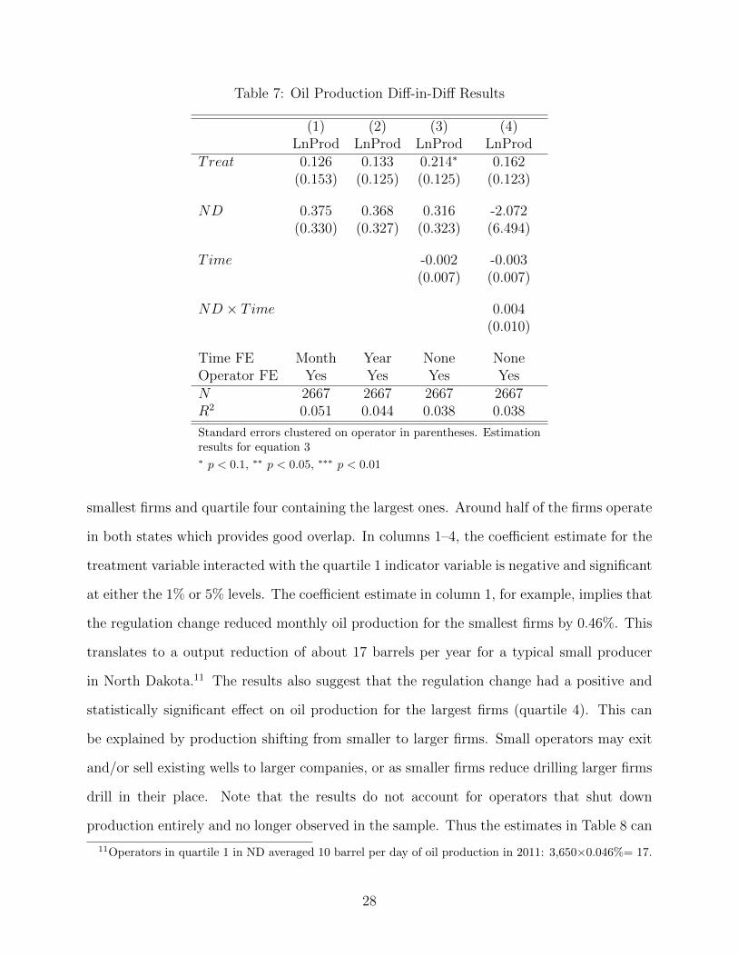
Table 7: Oil Production Diff-in-Diff Results
(1) (2) (3) (4)LnProd LnProd LnProd LnProd
Treat 0.126 0.133 0.214∗ 0.162(0.153) (0.125) (0.125) (0.123)
ND 0.375 0.368 0.316 -2.072(0.330) (0.327) (0.323) (6.494)
Time -0.002 -0.003(0.007) (0.007)
ND × Time 0.004(0.010)
Time FE Month Year None NoneOperator FE Yes Yes Yes YesN 2667 2667 2667 2667R2 0.051 0.044 0.038 0.038
Standard errors clustered on operator in parentheses. Estimationresults for equation 3∗ p < 0.1, ∗∗ p < 0.05, ∗∗∗ p < 0.01
smallest firms and quartile four containing the largest ones. Around half of the firms operate
in both states which provides good overlap. In columns 1–4, the coefficient estimate for the
treatment variable interacted with the quartile 1 indicator variable is negative and significant
at either the 1% or 5% levels. The coefficient estimate in column 1, for example, implies that
the regulation change reduced monthly oil production for the smallest firms by 0.46%. This
translates to a output reduction of about 17 barrels per year for a typical small producer
in North Dakota.11 The results also suggest that the regulation change had a positive and
statistically significant effect on oil production for the largest firms (quartile 4). This can
be explained by production shifting from smaller to larger firms. Small operators may exit
and/or sell existing wells to larger companies, or as smaller firms reduce drilling larger firms
drill in their place. Note that the results do not account for operators that shut down
production entirely and no longer observed in the sample. Thus the estimates in Table 8 can
11Operators in quartile 1 in ND averaged 10 barrel per day of oil production in 2011: 3,650×0.046%= 17.
28
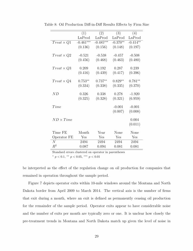
Table 8: Oil Production Diff-in-Diff Results Effects by Firm Size
(1) (2) (3) (4)LnProd LnProd LnProd LnProd
Treat×Q1 -0.461∗∗∗ -0.485∗∗∗ -0.370∗∗ -0.414∗∗
(0.136) (0.156) (0.148) (0.197)
Treat×Q2 -0.521 -0.538 -0.457 -0.508(0.456) (0.468) (0.463) (0.480)
Treat×Q3 0.209 0.192 0.287 0.239(0.416) (0.439) (0.417) (0.396)
Treat×Q4 0.753∗∗ 0.737∗∗ 0.829∗∗ 0.781∗∗
(0.334) (0.338) (0.335) (0.370)
ND 0.326 0.338 0.278 -1.920(0.325) (0.328) (0.321) (6.959)
Time -0.001 -0.001(0.007) (0.008)
ND × Time 0.004(0.011)
Time FE Month Year None NoneOperator FE Yes Yes Yes YesN 2494 2494 2494 2494R2 0.087 0.094 0.081 0.081
Standard errors clustered on operator in parentheses∗ p < 0.1, ∗∗ p < 0.05, ∗∗∗ p < 0.01
be interpreted as the effect of the regulation change on oil production for companies that
remained in operation throughout the sample period.
Figure 7 depicts operator exits within 10-mile windows around the Montana and North
Dakota border from April 2009 to March 2014. The vertical axis is the number of firms
that exit during a month, where an exit is defined as permanently ceasing oil production
for the remainder of the sample period. Operator exits appear to have considerable noise
and the number of exits per month are typically zero or one. It is unclear how closely the
pre-treatment trends in Montana and North Dakota match up given the level of noise in
29
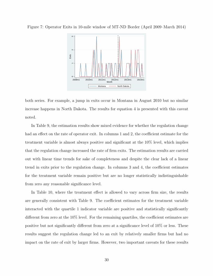
Figure 7: Operator Exits in 10-mile window of MT-ND Border (April 2009–March 2014)
01
23
Exi
ts
2009m1 2010m1 2011m1 2012m1 2013m1 2014m1Month
Montana North Dakota
both series. For example, a jump in exits occur in Montana in August 2010 but no similar
increase happens in North Dakota. The results for equation 4 is presented with this caveat
noted.
In Table 9, the estimation results show mixed evidence for whether the regulation change
had an effect on the rate of operator exit. In columns 1 and 2, the coefficient estimate for the
treatment variable is almost always positive and significant at the 10% level, which implies
that the regulation change increased the rate of firm exits. The estimation results are carried
out with linear time trends for sake of completeness and despite the clear lack of a linear
trend in exits prior to the regulation change. In columns 3 and 4, the coefficient estimates
for the treatment variable remain positive but are no longer statistically indistinguishable
from zero any reasonable significance level.
In Table 10, where the treatment effect is allowed to vary across firm size, the results
are generally consistent with Table 9. The coefficient estimates for the treatment variable
interacted with the quartile 1 indicator variable are positive and statistically significantly
different from zero at the 10% level. For the remaining quartiles, the coefficient estimates are
positive but not significantly different from zero at a significance level of 10% or less. These
results suggest the regulation change led to an exit by relatively smaller firms but had no
impact on the rate of exit by larger firms. However, two important caveats for these results
30
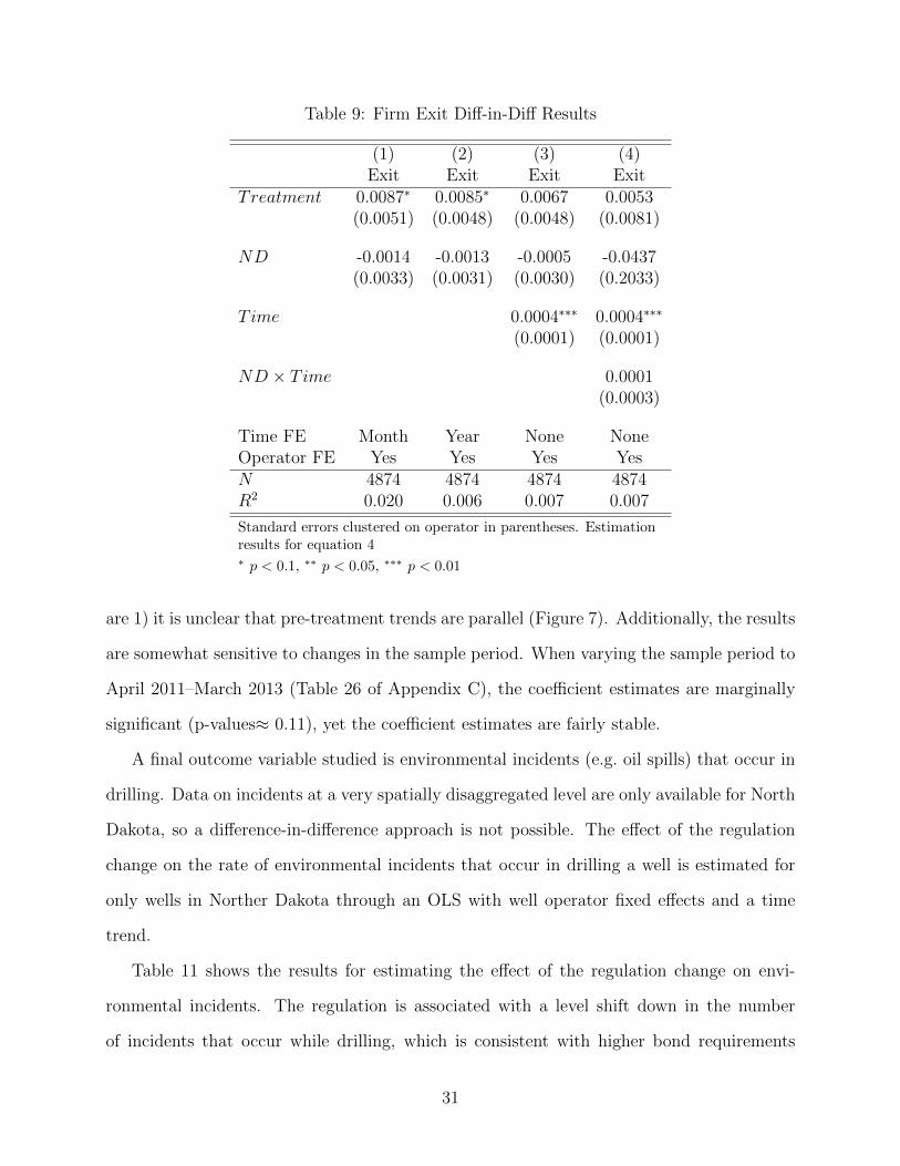
Table 9: Firm Exit Diff-in-Diff Results
(1) (2) (3) (4)Exit Exit Exit Exit
Treatment 0.0087∗ 0.0085∗ 0.0067 0.0053(0.0051) (0.0048) (0.0048) (0.0081)
ND -0.0014 -0.0013 -0.0005 -0.0437(0.0033) (0.0031) (0.0030) (0.2033)
Time 0.0004∗∗∗ 0.0004∗∗∗
(0.0001) (0.0001)
ND × Time 0.0001(0.0003)
Time FE Month Year None NoneOperator FE Yes Yes Yes YesN 4874 4874 4874 4874R2 0.020 0.006 0.007 0.007
Standard errors clustered on operator in parentheses. Estimationresults for equation 4∗ p < 0.1, ∗∗ p < 0.05, ∗∗∗ p < 0.01
are 1) it is unclear that pre-treatment trends are parallel (Figure 7). Additionally, the results
are somewhat sensitive to changes in the sample period. When varying the sample period to
April 2011–March 2013 (Table 26 of Appendix C), the coefficient estimates are marginally
significant (p-values≈ 0.11), yet the coefficient estimates are fairly stable.
A final outcome variable studied is environmental incidents (e.g. oil spills) that occur in
drilling. Data on incidents at a very spatially disaggregated level are only available for North
Dakota, so a difference-in-difference approach is not possible. The effect of the regulation
change on the rate of environmental incidents that occur in drilling a well is estimated for
only wells in Norther Dakota through an OLS with well operator fixed effects and a time
trend.
Table 11 shows the results for estimating the effect of the regulation change on envi-
ronmental incidents. The regulation is associated with a level shift down in the number
of incidents that occur while drilling, which is consistent with higher bond requirements
31
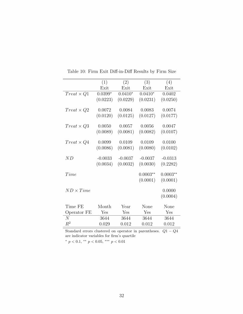
Table 10: Firm Exit Diff-in-Diff Results by Firm Size
(1) (2) (3) (4)Exit Exit Exit Exit
Treat×Q1 0.0399∗ 0.0410∗ 0.0410∗ 0.0402(0.0223) (0.0229) (0.0231) (0.0250)
Treat×Q2 0.0072 0.0084 0.0083 0.0074(0.0120) (0.0125) (0.0127) (0.0177)
Treat×Q3 0.0050 0.0057 0.0056 0.0047(0.0089) (0.0081) (0.0082) (0.0107)
Treat×Q4 0.0099 0.0109 0.0109 0.0100(0.0086) (0.0081) (0.0080) (0.0102)
ND -0.0033 -0.0037 -0.0037 -0.0313(0.0034) (0.0032) (0.0030) (0.2282)
Time 0.0003∗∗ 0.0003∗∗
(0.0001) (0.0001)
ND × Time 0.0000(0.0004)
Time FE Month Year None NoneOperator FE Yes Yes Yes YesN 3644 3644 3644 3644R2 0.029 0.012 0.012 0.012
Standard errors clustered on operator in parentheses. Q1 − Q4are indicator variables for firm’s quartile∗ p < 0.1, ∗∗ p < 0.05, ∗∗∗ p < 0.01
32
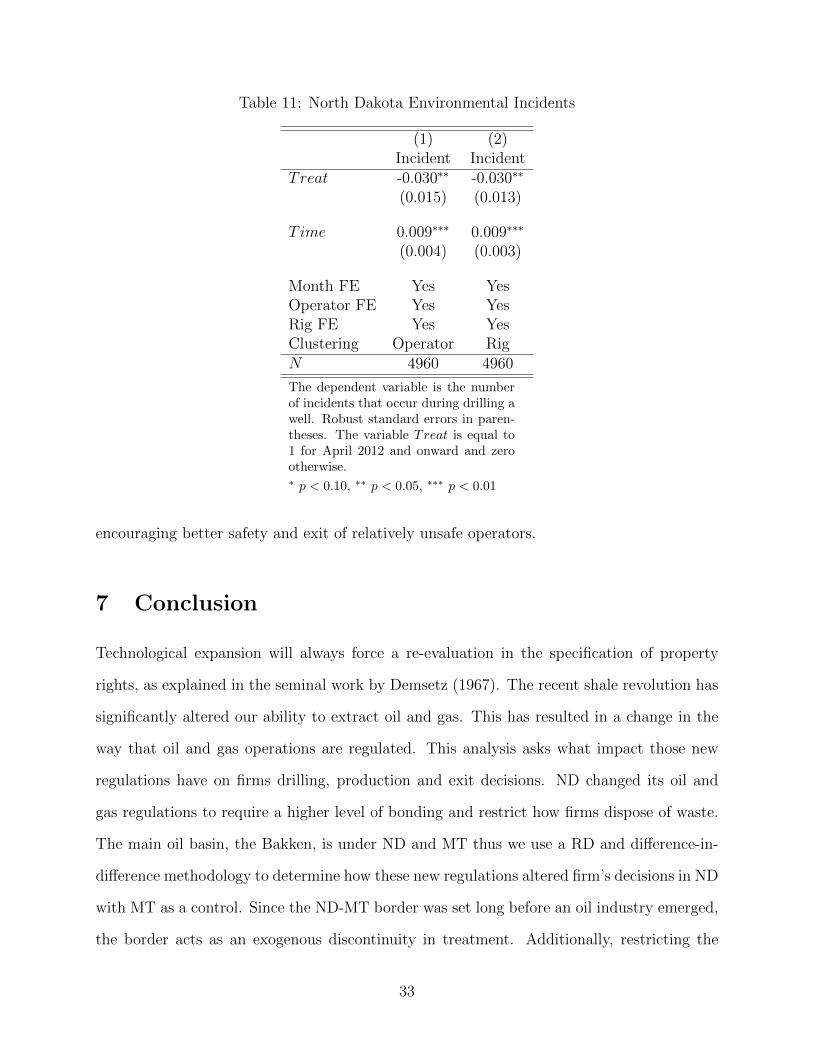
Table 11: North Dakota Environmental Incidents
(1) (2)Incident Incident
Treat -0.030∗∗ -0.030∗∗
(0.015) (0.013)
Time 0.009∗∗∗ 0.009∗∗∗
(0.004) (0.003)
Month FE Yes YesOperator FE Yes YesRig FE Yes YesClustering Operator RigN 4960 4960
The dependent variable is the numberof incidents that occur during drilling awell. Robust standard errors in paren-theses. The variable Treat is equal to1 for April 2012 and onward and zerootherwise.∗ p < 0.10, ∗∗ p < 0.05, ∗∗∗ p < 0.01
encouraging better safety and exit of relatively unsafe operators.
7 Conclusion
Technological expansion will always force a re-evaluation in the specification of property
rights, as explained in the seminal work by Demsetz (1967). The recent shale revolution has
significantly altered our ability to extract oil and gas. This has resulted in a change in the
way that oil and gas operations are regulated. This analysis asks what impact those new
regulations have on firms drilling, production and exit decisions. ND changed its oil and
gas regulations to require a higher level of bonding and restrict how firms dispose of waste.
The main oil basin, the Bakken, is under ND and MT thus we use a RD and difference-in-
difference methodology to determine how these new regulations altered firm’s decisions in ND
with MT as a control. Since the ND-MT border was set long before an oil industry emerged,
the border acts as an exogenous discontinuity in treatment. Additionally, restricting the
33
analysis to a short distance around the border helps ensure that other unobservables, like
geology, is constant.
Results find no change in the pace of drilling nor the level of oil production in ND
after the regulations passed relative to MT. However, this average effect masks a change in
organization in the oil industry in ND. Small operators are statistically more likely to exit
the area of analysis and to reduce the level of production. This effect is countered by an
increase in production from large operators. The results imply that larger firms may have
benefited from the regulation through reduction competition by raising their rivals costs, an
outcome predicted by Salop and Scheffman (1983). The amount of environmental accidents
related to oil drilling has decreased in ND since passage of these regulations, though this
result is not tested against the amount of MT accidents.
This analysis also provides useful information for policymakers weighing the costs and
benefits of increased environmental regulation. The potentially regulated firms usually ar-
gue that proposed regulations will threaten their activities in the relative jurisdiction and
argue that this will cost jobs and tax revenue. However, it is difficult for policymakers to
find rigorous, objective information on how firms have responded to previous environmental
regulations. In this case, the increase bonding requirements and restrictions on drilling waste
disposals did not change the pace of economic activity. Unfortunately, this analysis can not
reveal whether the change in industrial composition will have long-run consequences for the
oil industry in ND. The short-run consequences have been small, if any.
34
References
Randy Becker and Vernon Henderson. Effects of air quality regulations on polluting indus-
tries. Journal of Political Economy, 108(2):379–421, 2000.
John P. Bluemle. North dakota’s boundaries, 2007. URL https://www.dmr.nd.gov/ndgs/
ndnotes/boundaries/boundaries.asp.
Judson Boomhower. Drilling like theres no tomorrow: Bankruptcy, insurance, and environ-
mental risk. EI@ Haas Working Paper, 254, 2014.
James Cust and Torfinn Harding. Institutions and the location of oil exploration. Technical
report, Oxford Centre for the Analysis of Resource Rich Economies, University of Oxford,
2014.
Lucas W Davis. Bonding requirements for us natural gas producers. Review of Environmental
Economics and Policy, 9(1):128–144, 2015.
Harold Demsetz. Toward a theory of property rights. American Economic Review, 57(2):
347–359, 1967.
Drillinginfo, 2015. URL http://info.drillinginfo.com/.
U.S. EPA. Assessment of the potential impacts of hydraulic fracturing for oil and gas on
drinking water resources (external review draft), 2015. URL http://cfpub.epa.gov/
ncea/hfstudy/recordisplay.cfm?deid=244651.
C.E. Erdmann. Mineral and water resources of montana, n.d. URL http://www.mbmg.
mtech.edu/sp28/fuels.htm.
Andrew Gelman and Guido Imbens. Why high-order polynomials should not be used in
regression discontinuity designs. Technical report, National Bureau of Economic Research,
2014.
35
David Gerard. The law and economics of reclamation bonds. Resources Policy, 26(4):189 –
197, 2000. ISSN 0301-4207. doi: http://dx.doi.org/10.1016/S0301-4207(00)00033-7. URL
http://www.sciencedirect.com/science/article/pii/S0301420700000337.
Russell Gold. The boom: how fracking ignited the American energy revolution and changed
the world. Simon and Schuster, 2015.
Michael Greenstone. The impacts of environmental regulations on industrial activity: Evi-
dence from the 1970 and 1977 clean air act amendments and the census of manufacturers.
Journal of Political Economy, 110(6):1175–1219, 2002.
J. Vernon Henderson. Effects of air quality regulation. The American Economic Review, 86
(4):789–813, 1996. ISSN 00028282. URL http://www.jstor.org/stable/2118305.
Tracy Hume. Energy pipeline: Colorado’s oil production flips between fields, Jan-
uary 2015. URL http://www.greeleytribune.com/news/feature2/13743683-113/
oil-production-colorado-rangely.
Ryan Kellogg. The effect of uncertanty on investment: Evidence from texas oil drilling.
American Economic Review, 104(6):1698–1734, 2014.
Byung-Cheol Kim and Matt Oliver. Taming drillers through legislative action:evidence from
pennsylvania’s shale gas industry. Technical report, Mimeo, 2016.
Nicholas Kusnetz. North dakotas oil boom brings damage along with
prosperity, June 2012. URL http://www.propublica.org/article/
the-other-fracking-north-dakotas-oil-boom-brings-damage-along-with-prosperi.
David S. Lee and David Card. Regression discontinuity inference with specification er-
ror. Journal of Econometrics, 142(2):655 – 674, 2008. doi: http://dx.doi.org/10.1016/j.
jeconom.2007.05.003.
36
James MacPherson. Industry: New nd oil rules could curb drilling, 2012. URL http://www.
willistonherald.com/news/industry-new-nd-oil-rules-could-curb-drilling/
article_42e39e44-6f7c-11e1-b645-0019bb2963f4.html.
Peter Maniloff and Dale Manning. Division of nonrenewable resource rents: A model of asym-
metric nash competition with state control of heterogenous resources. Colorado School of
Mines Division of Economics and Business Working Paper 2015-08, 2015.
MBOGC. Hydraulic fracturing rulemaking, 2011. URL http://bogc.dnrc.mt.gov/frac.
asp.
MBOGC. Adminstrative rules of montana, 2016. URL http://bogc.dnrc.mt.gov/
rulesregs.asp.
Daniel L Millimet, Santanu Roy, and Aditi Sengupta. Environmental regulations and eco-
nomic activity: Influence on market structure. Annual Review of Resource Economics, 1,
2009.
NDGS. Overview of the petroleum geology of the north dakota williston basin, n.d. URL
https://www.dmr.nd.gov/ndgs/resources/.
NDIC. Proposed rule changes now final, 2012a. URL https://www.dmr.nd.gov/oilgas/
pressreleases/PressRelease03142012.pdfl.
NDIC. Rule changes for non-regulators north dakota 2012 rule changes effective april 1,
2012, 2012b. URL https://www.dmr.nd.gov/oilgas/RuleChanges2012NonReg.pdf.
NDIC. North dakota industrial commission rulebook, 2016. URL https://www.dmr.nd.
gov/oilgas/rules/rulebook.pdf.
NDPC. The association, 2012. URL https://www.ndoil.org/about_us/
the-association/.
37
NETL. Research on local and regional air quality impacts of oil and natural gas devel-
opment, 2014. URL https://www.netl.doe.gov/File%20Library/Research/onsite%
20research/R-D160-2014Sep-rev11-14.pdf.
Pedro Ramirez Jr. Reserve pit management: risks to migratory birds. Cheyenne (WY):
US Fish and Wildlife Service, 2009. URL http://www.fws.gov/mountain-prairie/
contaminants/documents/ReservePits.pdf.
Nathan D Richardson, Madeline Gottlieb, Alan Krupnick, and Hannah Wiseman. The state
of state shale gas regulation. Resources for the Future Washington, DC, 2013.
Steven C Salop and David T Scheffman. Raising rivals’ costs. The American Economic
Review, 73(2):267–271, 1983.
Society of Petroleum Engineers. Guidelines for the application of the petroleum re-
sources management system, 2011. URL http://www.spe.org/industry/docs/PRMS_
Guidelines_Nov2011.pdf.
State Historical Society of North Dakota. Mapping the land & its people - statehood map,
2016. URL http://history.nd.gov/textbook/unit1_natworld/unit1_2_statehood.
html.
Christopher Timmins and Ashley Vissing. Shale gas leases: Is bargaining efficient and what
are the implications for homeowners if it is not? Mimeo Duke University, 2014.
W. Reed Walker. The transitional costs of sectoral reallocation: Evidence from the clean air
act and the workforce. Quarterly Journal of Economics, forthcoming, 2013.
Coady Wing and Thomas D Cook. Strengthening the regression discontinuity design using
additional design elements: A within-study comparison. Journal of Policy Analysis and
Management, 32(4):853–877, 2013.
38
Appendix A
This appendix provides several variations of the RD design discussed in Section 5 and esti-
mates for a difference-in-difference model to complement the RD model. In general, mod-
ifications to the sample period, functional forms, and windows do not change the overall
conclusion that there is no evidence the regulation change affect drilling activity.
Tables 12 and 13 present expanded results for the RD estimation in equation 1. In
Table 12, the coefficient and standard errors estimates for the assignment variable are shown
for well drilling in the two-year period prior to the regulation revisions (April 2010–March
2012). Additionally, the AIC values for each model are included below the standard error
estimates. Table 13 presents the coefficient estimates for the sample period following the
regulation change (April 2012–March 2014). The window around the Montana-North Dakota
border is varied across the columns, and the rows reflect different polynomial orders for the
function f(xi) in equation 1.
Table 14 shows the estimation results for equation 2. The coefficient estimates for the
treatment variable (Djt) are presented along with the standard error estimates and AIC
values. The sample period for well drilling is April 2010 to March 2014. The columns are
different windows around the Montana-North Dakota border, and the rows are specifications
with varying polynomial orders.
Tables 15 and 16 contain non-parametric RD results for well drilling in the two years
before and two years following the regulation change. The results are generally consistent
with Tables 12 and 13 in showing no discontinuity in drilling at the border either prior to or
after the regulation revisions.
Table 17 presents the estimation results for equation 2 when the pre-treatment and post-
treatment sample periods are limited to April 2010–March 2011 and April 2013–March 2014,
respectively. This restricts the sample to drilling activity that occurred 12-24 months before
and 12–24 months after the regulation change. It allows for testing whether the regulation
had a delayed effect on well drilling. The results are fairly similar to Table 5; there are more
39
coefficient estimates that are negative but none are statistically significant.
Table 19 shows that the estimation results for equation 2, when the latitude fixed effect
(γi) is excluded, are fairly similar to the results with the fixed effects included.
Table 20 contains the estimation results for equation 2 when the cell size is modified
from 1x1 miles to 5x5 miles. The results show little evidence that the regulation revisions
had an effect on drilling. For only one window width (50 miles) and one polynomial func-
tion (cubic) is the coefficient estimate for the treatment variable negative and statistically
indistinguishable from zero.
Table 21 presents the estimation results for equation 1 with the number of wells drilled
within the cell in the prior two years (April 2010–March 2012) included as a control. This
allows for the possibility that the level of drilling activity within a cell before the regulation
change may affect subsequent drilling levels. Cells may have an existing well because they
are more economically attractive, and in turn experience more drilling in the following two
years. Additionally a cell may become saturated with wells and drilling within the cell may
decline. The number of wells previously drilled, and the squared number of wells previously
drilled are included as controls. The results consistent with other specifications that show
no evidence that the regulation influenced drilling.
Table ?? presents the estimation of a difference-in-differences model with the number
of wells drilled as the dependent variable. Results are shown across six different distances
around the ND-MT border. The implications are that within 10 miles of the border there
is no change in the number of wells drilled as a result of the well bonding requirements. As
the distance expands, the underlying geology favors ND and the results bear this out as the
results imply an increase in drilling in ND after the increase in well bonds.
40
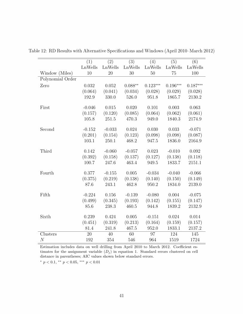
Table 12: RD Results with Alternative Specifications and Windows (April 2010–March 2012)
(1) (2) (3) (4) (5) (6)LnWells LnWells LnWells LnWells LnWells LnWells
Window (Miles) 10 20 30 50 75 100Polynomial Order
Zero 0.032 0.052 0.088∗∗ 0.123∗∗∗ 0.196∗∗∗ 0.187∗∗∗
(0.064) (0.041) (0.034) (0.028) (0.029) (0.028)192.9 330.0 526.0 951.8 1865.7 2130.2
First -0.046 0.015 0.020 0.101 0.003 0.063(0.157) (0.120) (0.085) (0.064) (0.062) (0.061)105.8 251.5 470.3 949.0 1840.3 2174.9
Second -0.152 -0.033 0.024 0.030 0.033 -0.071(0.201) (0.154) (0.123) (0.098) (0.098) (0.087)103.1 250.1 468.2 947.5 1836.0 2164.9
Third 0.142 -0.060 -0.057 0.023 -0.010 0.092(0.392) (0.158) (0.137) (0.127) (0.138) (0.118)100.7 247.6 463.4 949.5 1833.7 2151.1
Fourth 0.377 -0.155 0.005 -0.034 -0.040 -0.066(0.375) (0.219) (0.138) (0.140) (0.150) (0.149)
87.6 243.1 462.8 950.2 1834.0 2139.0
Fifth -0.224 0.156 -0.139 -0.080 0.004 -0.075(0.499) (0.345) (0.193) (0.142) (0.155) (0.147)
85.6 238.3 460.5 944.8 1839.2 2132.9
Sixth 0.239 0.424 0.005 -0.151 0.024 0.014(0.451) (0.319) (0.213) (0.164) (0.159) (0.157)
81.4 241.8 467.5 952.0 1833.1 2137.2Clusters 20 40 60 97 124 145N 192 354 546 964 1519 1724
Estimation includes data on well drilling from April 2010 to March 2012. Coefficient es-timates for the assignment variable (Dj) in equation 1. Standard errors clustered on celldistance in parentheses; AIC values shown below standard errors.∗ p < 0.1, ∗∗ p < 0.05, ∗∗∗ p < 0.01
41
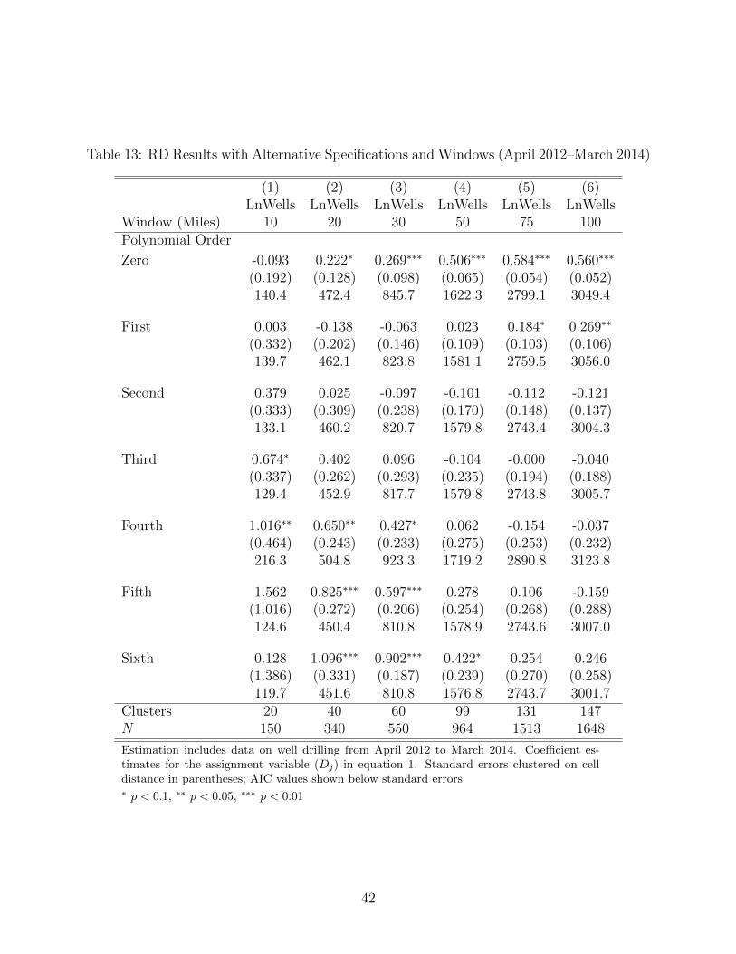
Table 13: RD Results with Alternative Specifications and Windows (April 2012–March 2014)
(1) (2) (3) (4) (5) (6)LnWells LnWells LnWells LnWells LnWells LnWells
Window (Miles) 10 20 30 50 75 100Polynomial Order
Zero -0.093 0.222∗ 0.269∗∗∗ 0.506∗∗∗ 0.584∗∗∗ 0.560∗∗∗
(0.192) (0.128) (0.098) (0.065) (0.054) (0.052)140.4 472.4 845.7 1622.3 2799.1 3049.4
First 0.003 -0.138 -0.063 0.023 0.184∗ 0.269∗∗
(0.332) (0.202) (0.146) (0.109) (0.103) (0.106)139.7 462.1 823.8 1581.1 2759.5 3056.0
Second 0.379 0.025 -0.097 -0.101 -0.112 -0.121(0.333) (0.309) (0.238) (0.170) (0.148) (0.137)133.1 460.2 820.7 1579.8 2743.4 3004.3
Third 0.674∗ 0.402 0.096 -0.104 -0.000 -0.040(0.337) (0.262) (0.293) (0.235) (0.194) (0.188)129.4 452.9 817.7 1579.8 2743.8 3005.7
Fourth 1.016∗∗ 0.650∗∗ 0.427∗ 0.062 -0.154 -0.037(0.464) (0.243) (0.233) (0.275) (0.253) (0.232)216.3 504.8 923.3 1719.2 2890.8 3123.8
Fifth 1.562 0.825∗∗∗ 0.597∗∗∗ 0.278 0.106 -0.159(1.016) (0.272) (0.206) (0.254) (0.268) (0.288)124.6 450.4 810.8 1578.9 2743.6 3007.0
Sixth 0.128 1.096∗∗∗ 0.902∗∗∗ 0.422∗ 0.254 0.246(1.386) (0.331) (0.187) (0.239) (0.270) (0.258)119.7 451.6 810.8 1576.8 2743.7 3001.7
Clusters 20 40 60 99 131 147N 150 340 550 964 1513 1648
Estimation includes data on well drilling from April 2012 to March 2014. Coefficient es-timates for the assignment variable (Dj) in equation 1. Standard errors clustered on celldistance in parentheses; AIC values shown below standard errors∗ p < 0.1, ∗∗ p < 0.05, ∗∗∗ p < 0.01
42
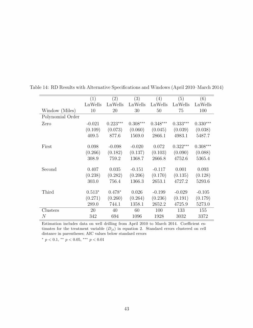
Table 14: RD Results with Alternative Specifications and Windows (April 2010–March 2014)
(1) (2) (3) (4) (5) (6)LnWells LnWells LnWells LnWells LnWells LnWells
Window (Miles) 10 20 30 50 75 100Polynomial Order
Zero -0.021 0.223∗∗∗ 0.308∗∗∗ 0.348∗∗∗ 0.333∗∗∗ 0.330∗∗∗
(0.109) (0.073) (0.060) (0.045) (0.039) (0.038)409.5 877.6 1569.0 2866.1 4983.1 5487.7
First 0.098 -0.098 -0.020 0.072 0.322∗∗∗ 0.308∗∗∗
(0.266) (0.182) (0.137) (0.103) (0.090) (0.088)308.9 759.2 1368.7 2666.8 4752.6 5365.4
Second 0.407 0.035 -0.151 -0.117 0.001 0.093(0.238) (0.282) (0.206) (0.170) (0.135) (0.128)303.0 756.4 1366.3 2653.1 4727.2 5293.6
Third 0.513∗ 0.478∗ 0.026 -0.199 -0.029 -0.105(0.271) (0.260) (0.264) (0.236) (0.191) (0.179)289.0 744.1 1358.1 2652.2 4725.9 5273.0
Clusters 20 40 60 100 133 155N 342 694 1096 1928 3032 3372
Estimation includes data on well drilling from April 2010 to March 2014. Coefficient es-timates for the treatment variable (Djt) in equation 2. Standard errors clustered on celldistance in parentheses; AIC values below standard errors∗ p < 0.1, ∗∗ p < 0.05, ∗∗∗ p < 0.01
43
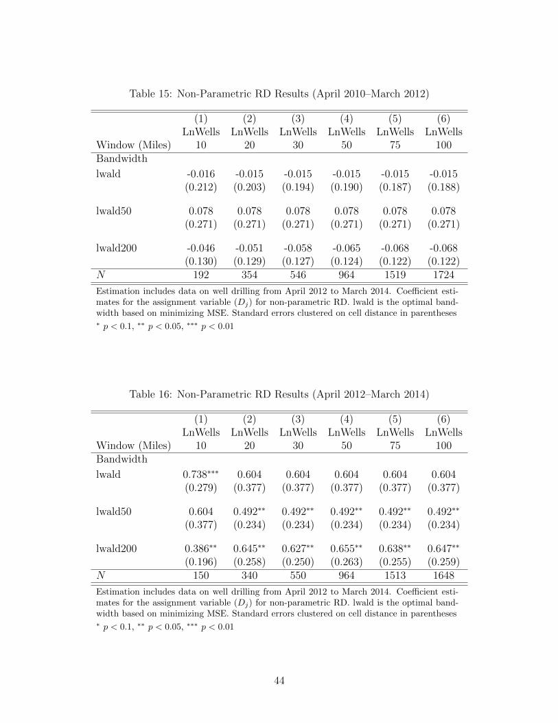
Table 15: Non-Parametric RD Results (April 2010–March 2012)
(1) (2) (3) (4) (5) (6)LnWells LnWells LnWells LnWells LnWells LnWells
Window (Miles) 10 20 30 50 75 100Bandwidth
lwald -0.016 -0.015 -0.015 -0.015 -0.015 -0.015(0.212) (0.203) (0.194) (0.190) (0.187) (0.188)
lwald50 0.078 0.078 0.078 0.078 0.078 0.078(0.271) (0.271) (0.271) (0.271) (0.271) (0.271)
lwald200 -0.046 -0.051 -0.058 -0.065 -0.068 -0.068(0.130) (0.129) (0.127) (0.124) (0.122) (0.122)
N 192 354 546 964 1519 1724
Estimation includes data on well drilling from April 2012 to March 2014. Coefficient esti-mates for the assignment variable (Dj) for non-parametric RD. lwald is the optimal band-width based on minimizing MSE. Standard errors clustered on cell distance in parentheses∗ p < 0.1, ∗∗ p < 0.05, ∗∗∗ p < 0.01
Table 16: Non-Parametric RD Results (April 2012–March 2014)
(1) (2) (3) (4) (5) (6)LnWells LnWells LnWells LnWells LnWells LnWells
Window (Miles) 10 20 30 50 75 100Bandwidth
lwald 0.738∗∗∗ 0.604 0.604 0.604 0.604 0.604(0.279) (0.377) (0.377) (0.377) (0.377) (0.377)
lwald50 0.604 0.492∗∗ 0.492∗∗ 0.492∗∗ 0.492∗∗ 0.492∗∗
(0.377) (0.234) (0.234) (0.234) (0.234) (0.234)
lwald200 0.386∗∗ 0.645∗∗ 0.627∗∗ 0.655∗∗ 0.638∗∗ 0.647∗∗
(0.196) (0.258) (0.250) (0.263) (0.255) (0.259)N 150 340 550 964 1513 1648
Estimation includes data on well drilling from April 2012 to March 2014. Coefficient esti-mates for the assignment variable (Dj) for non-parametric RD. lwald is the optimal band-width based on minimizing MSE. Standard errors clustered on cell distance in parentheses∗ p < 0.1, ∗∗ p < 0.05, ∗∗∗ p < 0.01
44
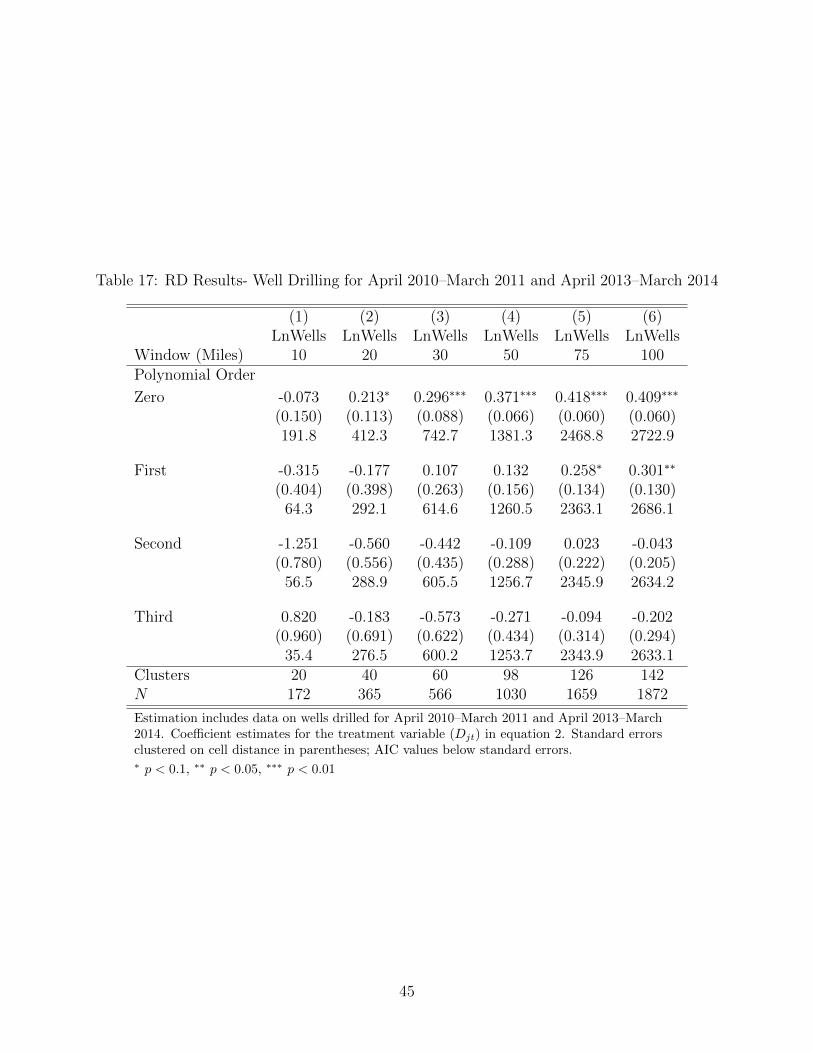
Table 17: RD Results- Well Drilling for April 2010–March 2011 and April 2013–March 2014
(1) (2) (3) (4) (5) (6)LnWells LnWells LnWells LnWells LnWells LnWells
Window (Miles) 10 20 30 50 75 100Polynomial Order
Zero -0.073 0.213∗ 0.296∗∗∗ 0.371∗∗∗ 0.418∗∗∗ 0.409∗∗∗
(0.150) (0.113) (0.088) (0.066) (0.060) (0.060)191.8 412.3 742.7 1381.3 2468.8 2722.9
First -0.315 -0.177 0.107 0.132 0.258∗ 0.301∗∗
(0.404) (0.398) (0.263) (0.156) (0.134) (0.130)64.3 292.1 614.6 1260.5 2363.1 2686.1
Second -1.251 -0.560 -0.442 -0.109 0.023 -0.043(0.780) (0.556) (0.435) (0.288) (0.222) (0.205)
56.5 288.9 605.5 1256.7 2345.9 2634.2
Third 0.820 -0.183 -0.573 -0.271 -0.094 -0.202(0.960) (0.691) (0.622) (0.434) (0.314) (0.294)
35.4 276.5 600.2 1253.7 2343.9 2633.1Clusters 20 40 60 98 126 142N 172 365 566 1030 1659 1872
Estimation includes data on wells drilled for April 2010–March 2011 and April 2013–March2014. Coefficient estimates for the treatment variable (Djt) in equation 2. Standard errorsclustered on cell distance in parentheses; AIC values below standard errors.∗ p < 0.1, ∗∗ p < 0.05, ∗∗∗ p < 0.01
45
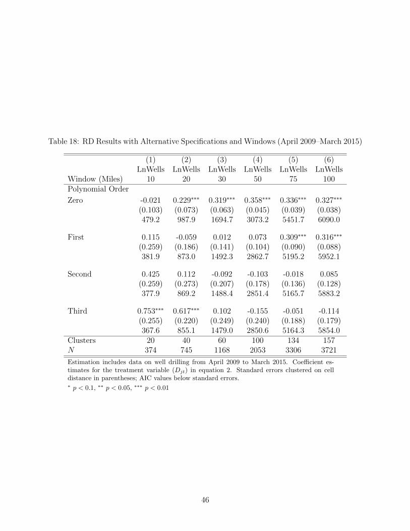
Table 18: RD Results with Alternative Specifications and Windows (April 2009–March 2015)
(1) (2) (3) (4) (5) (6)LnWells LnWells LnWells LnWells LnWells LnWells
Window (Miles) 10 20 30 50 75 100Polynomial Order
Zero -0.021 0.229∗∗∗ 0.319∗∗∗ 0.358∗∗∗ 0.336∗∗∗ 0.327∗∗∗
(0.103) (0.073) (0.063) (0.045) (0.039) (0.038)479.2 987.9 1694.7 3073.2 5451.7 6090.0
First 0.115 -0.059 0.012 0.073 0.309∗∗∗ 0.316∗∗∗
(0.259) (0.186) (0.141) (0.104) (0.090) (0.088)381.9 873.0 1492.3 2862.7 5195.2 5952.1
Second 0.425 0.112 -0.092 -0.103 -0.018 0.085(0.259) (0.273) (0.207) (0.178) (0.136) (0.128)377.9 869.2 1488.4 2851.4 5165.7 5883.2
Third 0.753∗∗∗ 0.617∗∗∗ 0.102 -0.155 -0.051 -0.114(0.255) (0.220) (0.249) (0.240) (0.188) (0.179)367.6 855.1 1479.0 2850.6 5164.3 5854.0
Clusters 20 40 60 100 134 157N 374 745 1168 2053 3306 3721
Estimation includes data on well drilling from April 2009 to March 2015. Coefficient es-timates for the treatment variable (Djt) in equation 2. Standard errors clustered on celldistance in parentheses; AIC values below standard errors.∗ p < 0.1, ∗∗ p < 0.05, ∗∗∗ p < 0.01
46
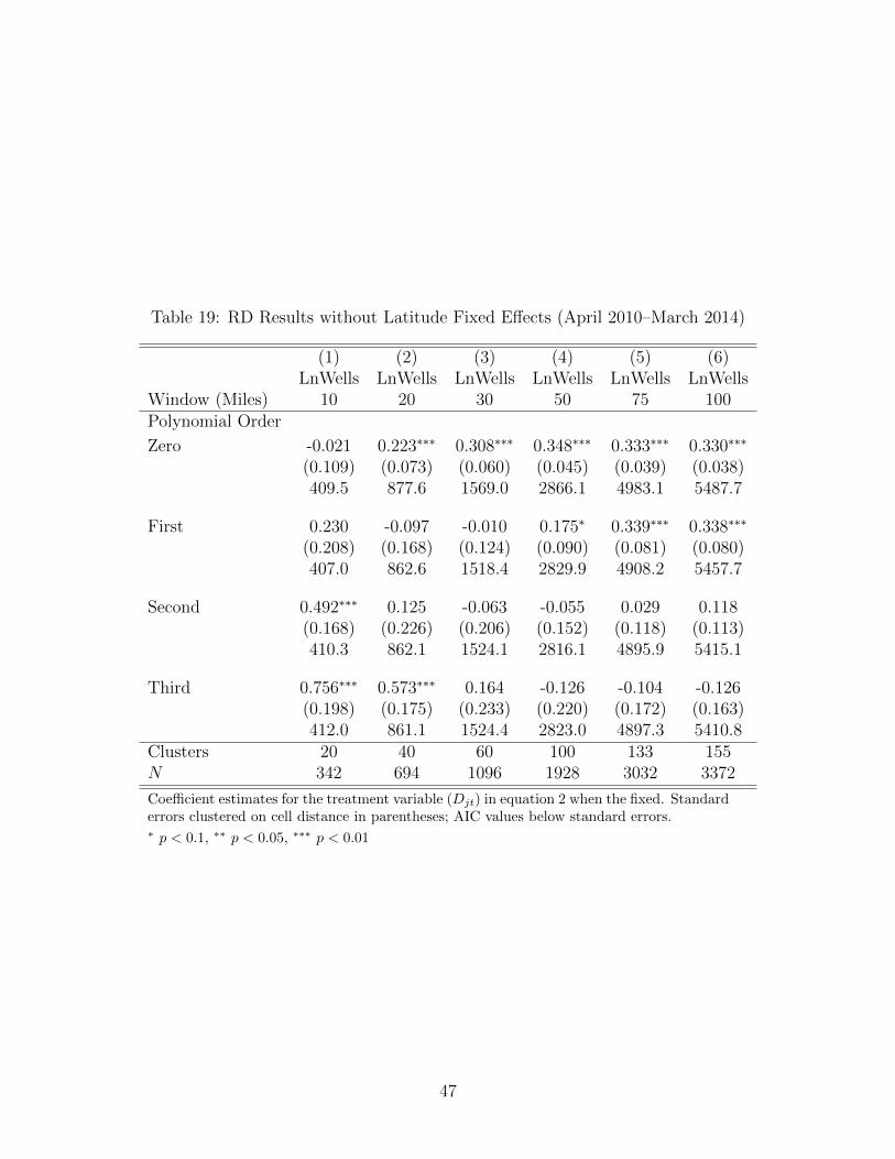
Table 19: RD Results without Latitude Fixed Effects (April 2010–March 2014)
(1) (2) (3) (4) (5) (6)LnWells LnWells LnWells LnWells LnWells LnWells
Window (Miles) 10 20 30 50 75 100Polynomial Order
Zero -0.021 0.223∗∗∗ 0.308∗∗∗ 0.348∗∗∗ 0.333∗∗∗ 0.330∗∗∗
(0.109) (0.073) (0.060) (0.045) (0.039) (0.038)409.5 877.6 1569.0 2866.1 4983.1 5487.7
First 0.230 -0.097 -0.010 0.175∗ 0.339∗∗∗ 0.338∗∗∗
(0.208) (0.168) (0.124) (0.090) (0.081) (0.080)407.0 862.6 1518.4 2829.9 4908.2 5457.7
Second 0.492∗∗∗ 0.125 -0.063 -0.055 0.029 0.118(0.168) (0.226) (0.206) (0.152) (0.118) (0.113)410.3 862.1 1524.1 2816.1 4895.9 5415.1
Third 0.756∗∗∗ 0.573∗∗∗ 0.164 -0.126 -0.104 -0.126(0.198) (0.175) (0.233) (0.220) (0.172) (0.163)412.0 861.1 1524.4 2823.0 4897.3 5410.8
Clusters 20 40 60 100 133 155N 342 694 1096 1928 3032 3372
Coefficient estimates for the treatment variable (Djt) in equation 2 when the fixed. Standarderrors clustered on cell distance in parentheses; AIC values below standard errors.∗ p < 0.1, ∗∗ p < 0.05, ∗∗∗ p < 0.01
47
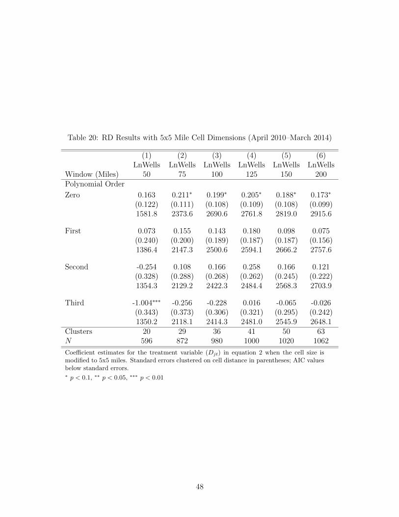
Table 20: RD Results with 5x5 Mile Cell Dimensions (April 2010–March 2014)
(1) (2) (3) (4) (5) (6)LnWells LnWells LnWells LnWells LnWells LnWells
Window (Miles) 50 75 100 125 150 200Polynomial Order
Zero 0.163 0.211∗ 0.199∗ 0.205∗ 0.188∗ 0.173∗
(0.122) (0.111) (0.108) (0.109) (0.108) (0.099)1581.8 2373.6 2690.6 2761.8 2819.0 2915.6
First 0.073 0.155 0.143 0.180 0.098 0.075(0.240) (0.200) (0.189) (0.187) (0.187) (0.156)1386.4 2147.3 2500.6 2594.1 2666.2 2757.6
Second -0.254 0.108 0.166 0.258 0.166 0.121(0.328) (0.288) (0.268) (0.262) (0.245) (0.222)1354.3 2129.2 2422.3 2484.4 2568.3 2703.9
Third -1.004∗∗∗ -0.256 -0.228 0.016 -0.065 -0.026(0.343) (0.373) (0.306) (0.321) (0.295) (0.242)1350.2 2118.1 2414.3 2481.0 2545.9 2648.1
Clusters 20 29 36 41 50 63N 596 872 980 1000 1020 1062
Coefficient estimates for the treatment variable (Djt) in equation 2 when the cell size ismodified to 5x5 miles. Standard errors clustered on cell distance in parentheses; AIC valuesbelow standard errors.∗ p < 0.1, ∗∗ p < 0.05, ∗∗∗ p < 0.01
48
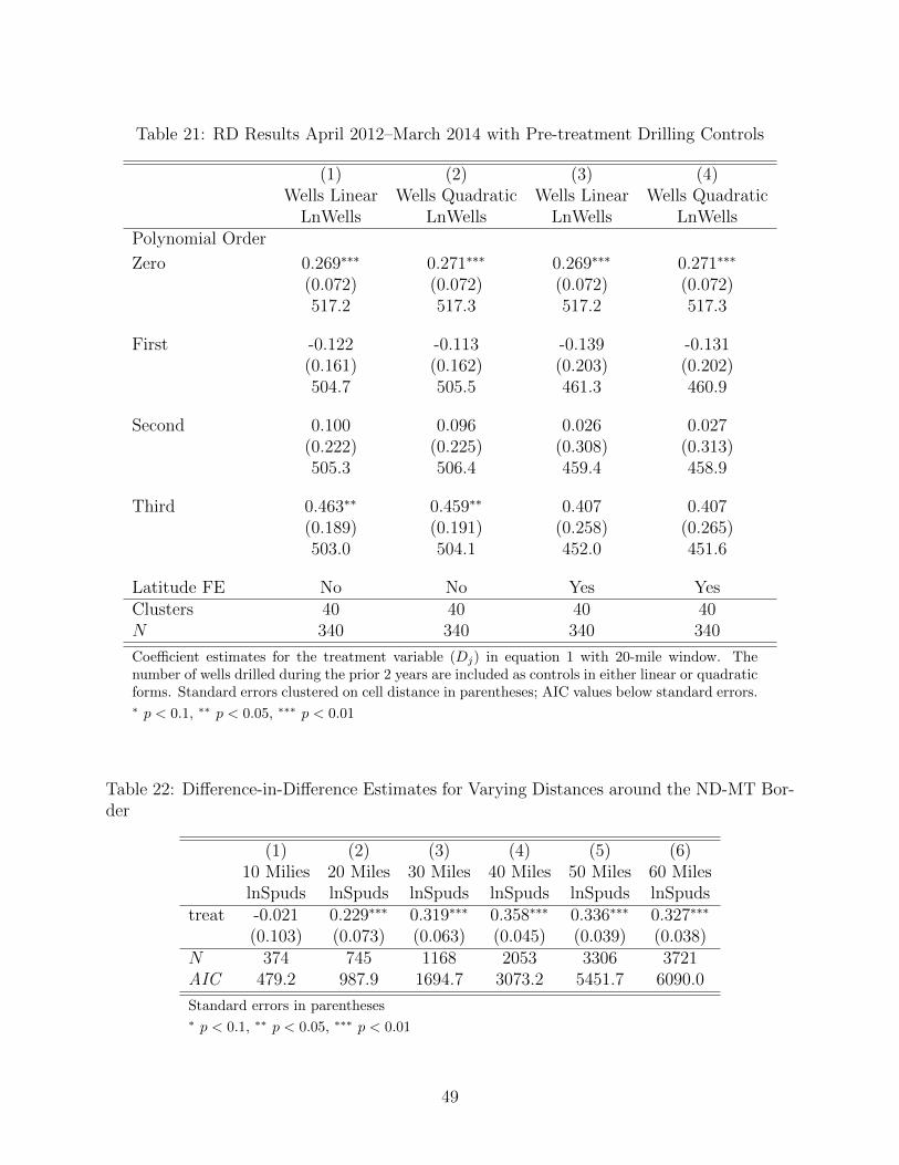
Table 21: RD Results April 2012–March 2014 with Pre-treatment Drilling Controls
(1) (2) (3) (4)Wells Linear Wells Quadratic Wells Linear Wells Quadratic
LnWells LnWells LnWells LnWellsPolynomial Order
Zero 0.269∗∗∗ 0.271∗∗∗ 0.269∗∗∗ 0.271∗∗∗
(0.072) (0.072) (0.072) (0.072)517.2 517.3 517.2 517.3
First -0.122 -0.113 -0.139 -0.131(0.161) (0.162) (0.203) (0.202)504.7 505.5 461.3 460.9
Second 0.100 0.096 0.026 0.027(0.222) (0.225) (0.308) (0.313)505.3 506.4 459.4 458.9
Third 0.463∗∗ 0.459∗∗ 0.407 0.407(0.189) (0.191) (0.258) (0.265)503.0 504.1 452.0 451.6
Latitude FE No No Yes YesClusters 40 40 40 40N 340 340 340 340
Coefficient estimates for the treatment variable (Dj) in equation 1 with 20-mile window. Thenumber of wells drilled during the prior 2 years are included as controls in either linear or quadraticforms. Standard errors clustered on cell distance in parentheses; AIC values below standard errors.∗ p < 0.1, ∗∗ p < 0.05, ∗∗∗ p < 0.01
Table 22: Difference-in-Difference Estimates for Varying Distances around the ND-MT Bor-der
(1) (2) (3) (4) (5) (6)10 Milies 20 Miles 30 Miles 40 Miles 50 Miles 60 MileslnSpuds lnSpuds lnSpuds lnSpuds lnSpuds lnSpuds
treat -0.021 0.229∗∗∗ 0.319∗∗∗ 0.358∗∗∗ 0.336∗∗∗ 0.327∗∗∗
(0.103) (0.073) (0.063) (0.045) (0.039) (0.038)N 374 745 1168 2053 3306 3721AIC 479.2 987.9 1694.7 3073.2 5451.7 6090.0
Standard errors in parentheses∗ p < 0.1, ∗∗ p < 0.05, ∗∗∗ p < 0.01
49
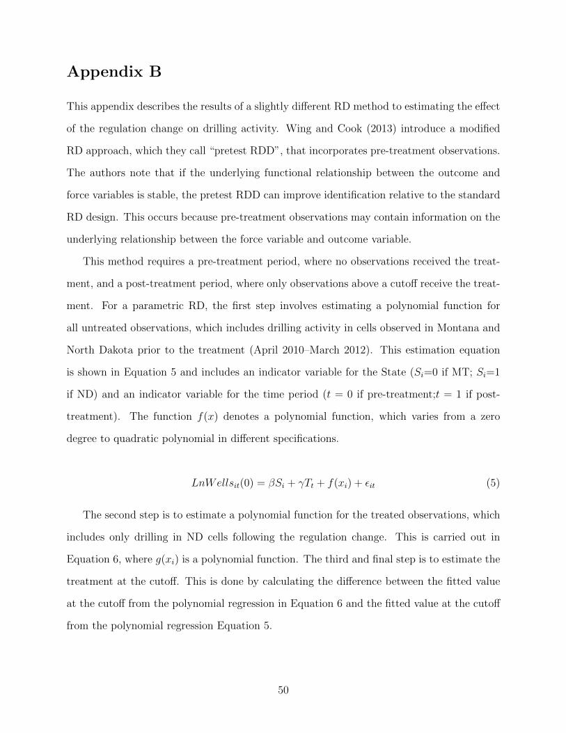
Appendix B
This appendix describes the results of a slightly different RD method to estimating the effect
of the regulation change on drilling activity. Wing and Cook (2013) introduce a modified
RD approach, which they call “pretest RDD”, that incorporates pre-treatment observations.
The authors note that if the underlying functional relationship between the outcome and
force variables is stable, the pretest RDD can improve identification relative to the standard
RD design. This occurs because pre-treatment observations may contain information on the
underlying relationship between the force variable and outcome variable.
This method requires a pre-treatment period, where no observations received the treat-
ment, and a post-treatment period, where only observations above a cutoff receive the treat-
ment. For a parametric RD, the first step involves estimating a polynomial function for
all untreated observations, which includes drilling activity in cells observed in Montana and
North Dakota prior to the treatment (April 2010–March 2012). This estimation equation
is shown in Equation 5 and includes an indicator variable for the State (Si=0 if MT; Si=1
if ND) and an indicator variable for the time period (t = 0 if pre-treatment;t = 1 if post-
treatment). The function f(x) denotes a polynomial function, which varies from a zero
degree to quadratic polynomial in different specifications.
LnWellsit(0) = βSi + γTt + f(xi) + εit (5)
The second step is to estimate a polynomial function for the treated observations, which
includes only drilling in ND cells following the regulation change. This is carried out in
Equation 6, where g(xi) is a polynomial function. The third and final step is to estimate the
treatment at the cutoff. This is done by calculating the difference between the fitted value
at the cutoff from the polynomial regression in Equation 6 and the fitted value at the cutoff
from the polynomial regression Equation 5.
50
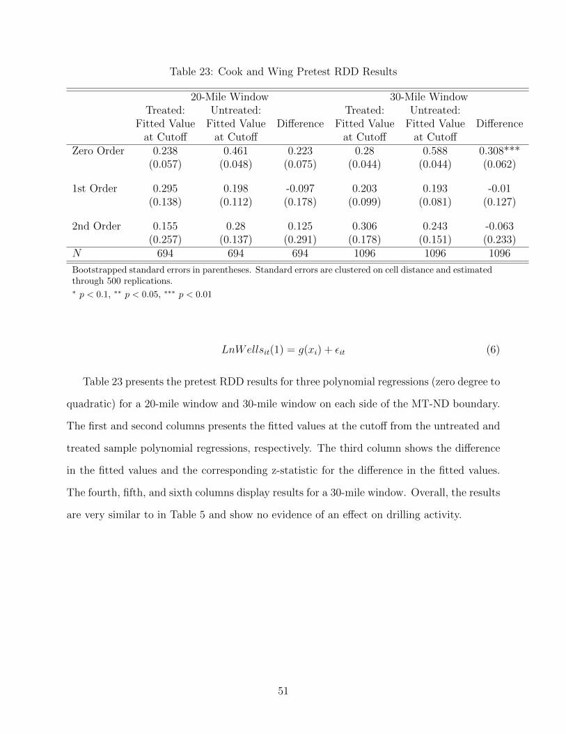
Table 23: Cook and Wing Pretest RDD Results
20-Mile Window 30-Mile WindowTreated: Untreated: Treated: Untreated:
Fitted Value Fitted Value Difference Fitted Value Fitted Value Differenceat Cutoff at Cutoff at Cutoff at Cutoff
Zero Order 0.238 0.461 0.223 0.28 0.588 0.308***(0.057) (0.048) (0.075) (0.044) (0.044) (0.062)
1st Order 0.295 0.198 -0.097 0.203 0.193 -0.01(0.138) (0.112) (0.178) (0.099) (0.081) (0.127)
2nd Order 0.155 0.28 0.125 0.306 0.243 -0.063(0.257) (0.137) (0.291) (0.178) (0.151) (0.233)
N 694 694 694 1096 1096 1096
Bootstrapped standard errors in parentheses. Standard errors are clustered on cell distance and estimatedthrough 500 replications.∗ p < 0.1, ∗∗ p < 0.05, ∗∗∗ p < 0.01
LnWellsit(1) = g(xi) + εit (6)
Table 23 presents the pretest RDD results for three polynomial regressions (zero degree to
quadratic) for a 20-mile window and 30-mile window on each side of the MT-ND boundary.
The first and second columns presents the fitted values at the cutoff from the untreated and
treated sample polynomial regressions, respectively. The third column shows the difference
in the fitted values and the corresponding z-statistic for the difference in the fitted values.
The fourth, fifth, and sixth columns display results for a 30-mile window. Overall, the results
are very similar to in Table 5 and show no evidence of an effect on drilling activity.
51

Appendix C
52

Table 24: Oil Production Diff-in-Diff Results- Effects by Firm Size (April 2010–March 2013)
(1) (2) (3) (4) (5)LnProd LnProd LnProd LnProd LnProd
Treat×Q1 -0.400∗∗∗ -0.374∗∗ -0.347∗∗ -0.671∗∗∗ -0.672∗∗∗
(0.138) (0.158) (0.141) (0.195) (0.197)
Treat×Q2 -0.354 -0.332 -0.335 -0.700 -0.659(0.414) (0.426) (0.415) (0.428) (0.433)
Treat×Q3 0.525 0.546 0.562 0.219 0.236(0.412) (0.433) (0.409) (0.364) (0.364)
Treat×Q4 1.012∗∗∗ 1.035∗∗∗ 1.046∗∗∗ 0.697∗ 0.714∗
(0.351) (0.358) (0.349) (0.357) (0.359)
ND 0.116 0.106 0.101 -11.242∗∗ -207.974(0.307) (0.310) (0.305) (5.476) (169.255)
Time 0.003 -0.000 0.255(0.006) (0.006) (0.301)
ND × Time 0.018∗∗ 0.648(0.009) (0.541)
Time2 -0.000(0.000)
ND × Time2 -0.001(0.000)
Time FE Month Year None None NoneOperator FE Yes Yes Yes Yes YesN 3306 3306 3306 3306 3306R2 0.085 0.095 0.080 0.085 0.091
Table shows results for equation 3 with the sample period varied. Standarderrors clustered on operator are shown in parentheses. The dependent variableis the natural log of monthly oil production. The sample period is April 2010 toMarch 2013. Q1, Q2, Q3, and Q4 are indicator variables for firm size quartiles∗ p < 0.1, ∗∗ p < 0.05, ∗∗∗ p < 0.01
53
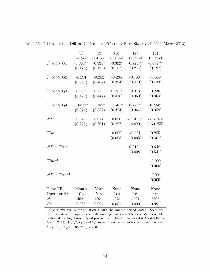
Table 25: Oil Production Diff-in-Diff Results- Effects by Firm Size (April 2009–March 2013)
(1) (2) (3) (4) (5)LnProd LnProd LnProd LnProd LnProd
Treat×Q1 -0.364∗∗ -0.326∗ -0.322∗ -0.725∗∗∗ -0.672∗∗∗
(0.170) (0.190) (0.163) (0.214) (0.197)
Treat×Q2 -0.294 -0.262 -0.284 -0.730∗ -0.659(0.395) (0.407) (0.394) (0.419) (0.433)
Treat×Q3 0.696 0.730 0.725∗ 0.313 0.236(0.426) (0.447) (0.416) (0.369) (0.364)
Treat×Q4 1.142∗∗∗ 1.175∗∗∗ 1.166∗∗∗ 0.740∗∗ 0.714∗
(0.374) (0.382) (0.374) (0.364) (0.359)
ND 0.029 0.017 0.020 -11.411∗∗ -207.974(0.298) (0.301) (0.297) (4.820) (169.255)
Time 0.002 -0.001 0.255(0.005) (0.005) (0.301)
ND × Time 0.019∗∗ 0.648(0.008) (0.541)
Time2 -0.000(0.000)
ND × Time2 -0.001(0.000)
Time FE Month Year None None NoneOperator FE Yes Yes Yes Yes YesN 4021 4021 4021 4021 3306R2 0.085 0.094 0.081 0.090 0.091
Table shows results for equation 3 with the sample period varied. Standarderrors clustered on operator are shown in parentheses. The dependent variableis the natural log of monthly oil production. The sample period is April 2009 toMarch 2013. Q1, Q2, Q3, and Q4 are indicator variables for firm size quartiles.∗ p < 0.1, ∗∗ p < 0.05, ∗∗∗ p < 0.01
54

Table 26: Firm Exit Diff-in-Diff Results- Effects by Firm Size (April 2011–March 2013)
(1) (2) (3) (4)Exit Exit Exit Exit
Treat×Q1 0.0404 0.0430 0.0429 0.0428(0.0253) (0.0261) (0.0265) (0.0290)
Treat×Q2 0.0052 0.0078 0.0075 0.0074(0.0141) (0.0145) (0.0147) (0.0217)
Treat×Q3 0.0044 0.0066 0.0063 0.0061(0.0106) (0.0093) (0.0095) (0.0130)
Treat×Q4 0.0087 0.0111 0.0109 0.0108(0.0100) (0.0090) (0.0087) (0.0124)
ND -0.0013 -0.0028 -0.0026 -0.0088(0.0057) (0.0051) (0.0049) (0.4128)
Time 0.0005∗∗ 0.0005∗∗
(0.0002) (0.0002)
ND × Time 0.0000(0.0007)
Time FE Month Year None NoneOperator FE Yes Yes Yes YesN 2639 2639 2639 2639R2 0.029 0.011 0.011 0.011
Table shows results for equation 4 with the sample period varied. Standarderrors clustered on operator are shown in parentheses. The dependent variableis an indicator variable for operator exit from state. The sample period is April2011 to March 2013. Q1, Q2, Q3, and Q4 are indicator variables for firm sizequartiles.∗ p < 0.1, ∗∗ p < 0.05, ∗∗∗ p < 0.01
55
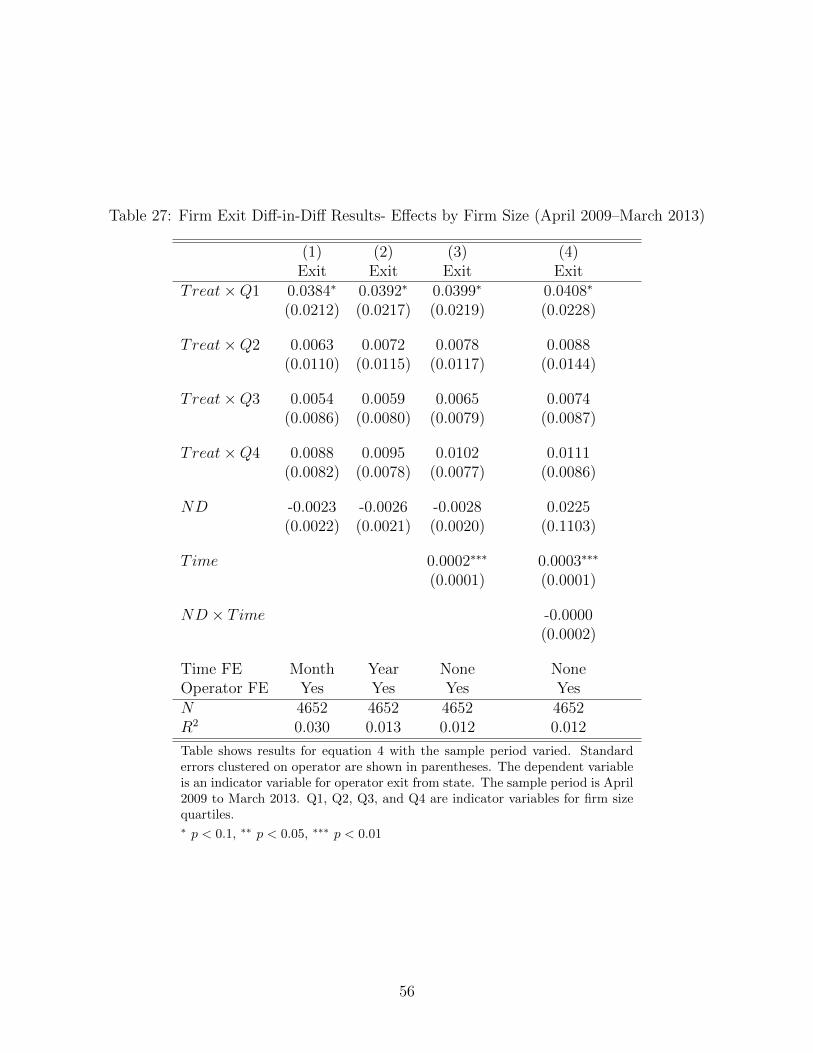
Table 27: Firm Exit Diff-in-Diff Results- Effects by Firm Size (April 2009–March 2013)
(1) (2) (3) (4)Exit Exit Exit Exit
Treat×Q1 0.0384∗ 0.0392∗ 0.0399∗ 0.0408∗
(0.0212) (0.0217) (0.0219) (0.0228)
Treat×Q2 0.0063 0.0072 0.0078 0.0088(0.0110) (0.0115) (0.0117) (0.0144)
Treat×Q3 0.0054 0.0059 0.0065 0.0074(0.0086) (0.0080) (0.0079) (0.0087)
Treat×Q4 0.0088 0.0095 0.0102 0.0111(0.0082) (0.0078) (0.0077) (0.0086)
ND -0.0023 -0.0026 -0.0028 0.0225(0.0022) (0.0021) (0.0020) (0.1103)
Time 0.0002∗∗∗ 0.0003∗∗∗
(0.0001) (0.0001)
ND × Time -0.0000(0.0002)
Time FE Month Year None NoneOperator FE Yes Yes Yes YesN 4652 4652 4652 4652R2 0.030 0.013 0.012 0.012
Table shows results for equation 4 with the sample period varied. Standarderrors clustered on operator are shown in parentheses. The dependent variableis an indicator variable for operator exit from state. The sample period is April2009 to March 2013. Q1, Q2, Q3, and Q4 are indicator variables for firm sizequartiles.∗ p < 0.1, ∗∗ p < 0.05, ∗∗∗ p < 0.01
56
Appendix D
This appendix provides the results of a duration analysis approach to estimating the effects of
the regulation change on firm exit. Duration analysis (or hazard modeling) is well suited for
evaluating firm exit because it allows the rate of exit to be time dependent and can account
for censored data. Equation 7 is a Cox proportional hazard model for an operator’s exit from
a state. An operator is considered to exit a state when they shutdown production within the
10-mile window of the MT-ND boundary and do not restart production for the remainder
of the sample period. The hazard function and baseline hazard function are denoted by h(t)
and h0(t), respectively. The variable D is the treatment variable, which is equal to one for
operator production in North Dakota and equal to zero for operator production in Montana.
h(t) = h0(t)exp(βD) (7)
Table 28 presents the results of four variations of the Cox proportional hazard model
in Equation 7. This table shows exponentiated coefficient estimates, where a value greater
than one in suggests there is a positive correlation between the regulation change and the
probability of firm exit; conversely, a coefficient estimate less than one implies the a negative
correlation with the probability of exit (i.e. prolongs the survival of the firm). Column 1,
which presents the hazard model results with the treatment dummy as the sole explanatory
variable, shows the regulation change is associated with a higher rate of firm exit. In column
2, where the baseline hazard function (h0(t)) is allowed to vary by operator, the coefficient
estimate for the treatment variable is similar and statistically significant at the 10% level.
Columns three and four assess whether the effects of the regulation on firm exit differ
across firm size. Firm size is measured as the operator’s total oil production in 2011, which is
prior to the regulation change. An ideal measure would be the value of a firm’s total assets,
but this information is not available for most of the operators in the dataset. Operators are
partitioned into quartiles based on their total oil production in Montana and North Dakota
57
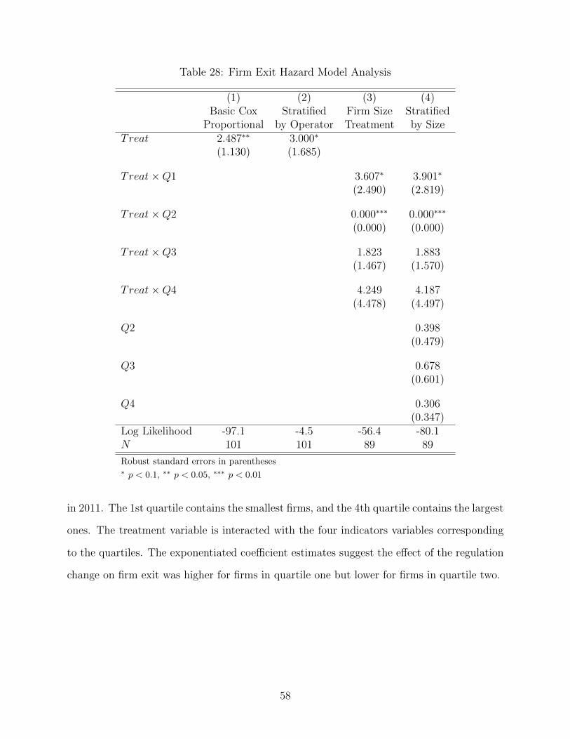
Table 28: Firm Exit Hazard Model Analysis
(1) (2) (3) (4)Basic Cox Stratified Firm Size Stratified
Proportional by Operator Treatment by SizeTreat 2.487∗∗ 3.000∗
(1.130) (1.685)
Treat×Q1 3.607∗ 3.901∗
(2.490) (2.819)
Treat×Q2 0.000∗∗∗ 0.000∗∗∗
(0.000) (0.000)
Treat×Q3 1.823 1.883(1.467) (1.570)
Treat×Q4 4.249 4.187(4.478) (4.497)
Q2 0.398(0.479)
Q3 0.678(0.601)
Q4 0.306(0.347)
Log Likelihood -97.1 -4.5 -56.4 -80.1N 101 101 89 89
Robust standard errors in parentheses∗ p < 0.1, ∗∗ p < 0.05, ∗∗∗ p < 0.01
in 2011. The 1st quartile contains the smallest firms, and the 4th quartile contains the largest
ones. The treatment variable is interacted with the four indicators variables corresponding
to the quartiles. The exponentiated coefficient estimates suggest the effect of the regulation
change on firm exit was higher for firms in quartile one but lower for firms in quartile two.
58