Divide and Conquer Local Average Regression

Xiangyu Chang1, Shaobo Lin2∗ and Yao Wang3

1Center of Data Science and Information Quality, School of Management, Xi’an

Jiaotong University, Xi’an, China

2Department of Statistics, College of Mathematics and Information Science, Wenzhou

University, Wenzhou, China

3 Department of Statistics, School of Mathematics and Statistics, Xi’an Jiaotong

University, Xi’an, China

This Version: March 15, 2016

Abstract

The divide and conquer strategy, which breaks a massive data set into a se-ries of manageable data blocks, and then combines the independent results ofdata blocks to obtain a final decision, has been recognized as a state-of-the-artmethod to overcome challenges of massive data analysis. In this paper, we mergethe divide and conquer strategy with local average regression methods to inferthe regressive relationship of input-output pairs from a massive data set. Aftertheoretically analyzing the pros and cons, we find that although the divide andconquer local average regression can reach the optimal learning rate, the restric-tion to the number of data blocks is a bit strong, which makes it only feasiblefor small number of data blocks. We then propose two variants to lessen (orremove) this restriction. Our results show that these variants can achieve theoptimal learning rate with much milder restriction (or without such restriction).Extensive experimental studies are carried out to verify our theoretical assertions.

KEY WORDS: Divide and Conquer Strategy, Local Average Regres-sion, Nadaraya-Watson Estimate, k Nearest Neighbor Estimate

∗∗Correspondence Author: sblin1983@gmail.com

1

arX

iv:1

601.

0623

9v2

[cs

.LG

] 1

3 M

ar 2

016

1 Introduction

Rapid expansion of capacity in the automatic data generation and acquisition has

made a profound impact on statistics and machine learning, as it brings data in un-

precedented size and complexity. These data are generally called as the “massive data”

or “big data” (Wu et al., 2014). Massive data bring new opportunities of discovering

subtle population patterns and heterogeneities which are believed to embody rich values

and impossible to be found in relatively small data sets. It, however, simultaneously

leads to a series of challenges such as the storage bottleneck, efficient computation,

etc. (Zhou et al., 2014).

To attack the aforementioned challenges, a divide and conquer strategy was sug-

gested and widely used in statistics and machine learning communities (Li et al., 2013;

Mcdonald et al., 2009; Zhang et al., 2013, 2015; Dwork and Smith, 2009; Battey et al.,

2015; Wang et al., 2015). This approach firstly distributes a massive data set into m

data blocks, then runs a specified learning algorithm on each data block independently

to get a local estimate fj, j = 1, . . . ,m and at last transmits m local estimates into one

machine to synthesize a global estimate f , which is expected to model the structure of

original massive dataset. A practical and exclusive synthesizing method is the average

mixture (AVM) (Li et al., 2013; Mcdonald et al., 2009; Zhang et al., 2013, 2015; Dwork

and Smith, 2009; Battey et al., 2015), i.e., f = 1m

∑mj=1 fj.

In practice, the above divide and conquer strategy has many applicable scenarios.

We show the following three situations as motivated examples. The first one is using

limited primary memory to handle a massive data set. In this situation, the divide and

conquer strategy is employed as a two-stage procedure. In the first stage, it reads the

whole data set sequentially block by block, each having a manageable sample size for

2

the limited primary memory, and derives a local estimate based on each block. In the

second stage, it averages local estimates to build up a global estimate (Li et al., 2013).

The second motivated example is using distributed data management systems to tackle

massive data. In this situation, distributed data management systems (e.g., Hadoop)

are designed by the divide and conquer strategy. They can load the whole data set

into the systems and tackle computational tasks separably and automatically. Guha

et al. (2012) has developed an integrated programing environment of R and Hadoop

(called RHIPE) for expedient and efficient statistical computing. The third motivated

example is the massive data privacy. In this situation, it divides a massive data set into

several small pieces and combining the estimates derived from these pieces for keeping

the data privacy (Dwork and Smith, 2009).

For nonparametric regression, the aforementioned divide and conquer strategy has

been shown to be efficient and feasible for global modeling methods such as the kernel

ridge regression (Zhang et al., 2015) and conditional maximum entropy model (Mcdon-

ald et al., 2009). Compared with the global modeling methods, local average regression

(LAR) (Gyorfi et al., 2002; Fan, 2000; Tsybakov, 2008), such as the Nadaraya-Watson

kernel (NWK) and k nearest neighbor (KNN) estimates, benefits in computation and

therefore, is also widely used in image processing (Takeda et al., 2007), power predic-

tion (Kramer et al., 2010), recommendation system (Biau et al., 2010) and financial

engineering (Kato, 2012). LAR is by definition a learning scheme that averages outputs

whose corresponding inputs satisfy certain localization assumptions. To tackle massive

data regression problems, we combine the divide and conquer approach with LAR to

produce a new learning scheme, average mixture local average regression (AVM-LAR),

just as Zhang et al. (2015) did for kernel ridge regression.

Our first purpose is to analyze the performance of AVM-LAR. After providing the

3

optimal learning rate of LAR, we show that AVM-LAR can also achieve this rate,

provided the number of data blocks, m, is relatively small. We also prove that the

restriction concerning m cannot be essentially improved. In a word, we provide both

the optimal learning rate and the essential restriction concerning m to guarantee the

optimal rate of AVM-LAR. It should be highlighted that this essential restriction is a

bit strong and makes AVM-LAR feasible only for small m. Therefore, compared with

LAR, AVM-LAR does not bring the essential improvement, since we must pay much

attention to determine an appropriate m.

Our second purpose is to pursue other divide and conquer strategies to equip LAR

efficiently. In particular, we provide two concrete variants of AVM-LAR in this paper.

The first variant is motivated by the distinction between KNN and NWK. In our

experiments, we note that the range of m to guarantee the optimal learning rate of

AVM-KNN is much larger than AVM-NWK. Recalling that the localization parameter

of KNN depends on data, while it doesn’t hold for NWK, we propose a variant of

AVM-LAR such that localization parameters of each data block depend on data. We

establish the optimal learning rate of this variant with mild restriction to m and verify

its feasibility by numerical simulations. The second variant is based on the definitions

of AVM and LAR. It follows from the definition of LAR that the predicted value of

a new input depends on samples near the input. If there are not such samples in a

specified data block, then this data block doesn’t affect the prediction of LAR. However,

AVM averages local estimates directly, neglecting the concrete value of a specified local

estimate, which may lead to an inaccurate prediction. Based on this observation, we

propose another variant of AVM-LAR by distinguishing whether a specified data block

affects the prediction. We provide the optimal learning rate of this variant without

any restriction to m and also present the experimental verifications.

4

To complete the above missions, the rest of paper is organized as follows. In Section

2, we present optimal learning rates of LAR and AVM-LAR and analyze the pros and

cons of AVM-LAR. In Section 3, we propose two new modified AVM-LARs to improve

the performance of AVM-LAR. A set of simulation studies to support the correctness

of our assertions are given in Section 4. In Section 5, we detailedly justify all the

theorems. In Section 6, we present the conclusion and some useful remarks.

2 Divide and Conquer Local Average Regression

In this section, after introducing some basic concepts of LAR, we present a baseline

of our analysis, where an optimal minimax learning rate of LAR is derived. Then, we

deduce the learning rate of AVM-LAR and analyze its pros and cons.

2.1 Local Average Regression

Let D = {(Xi, Yi)}Ni=1 be the data set where Xi ∈ X ⊆ Rd is a covariant and Yi ∈

[−M,M ] is the real-valued response. We always assume X is a compact set. Suppose

that samples are drawn independently and identically according to an unknown joint

distribution ρ over X × [−M,M ]. Then the main aim of nonparametric regression is

to construct a function f : X → [−M,M ] that can describe future responses based on

new inputs. The quality of the estimate f is measured in terms of the mean-squared

prediction error E{f(X)−Y }2, which is minimized by the so-called regression function

fρ(x) = E {Y |X = x}.

LAR, as one of the most widely used nonparametric regression approaches, con-

5

structs an estimate formed as

fD,h(x) =N∑i=1

Wh,Xi(x)Yi, (2.1)

where the localization weight Wh,Xi satisfies Wh,Xi(x) > 0 and∑N

i=1Wh,Xi(x) = 1.

Here, h > 0 is the so-called localization parameter. Generally speaking, Wh,Xi(x) is

“small” if Xi is “far” from x. Two widely used examples of LAR are Nadaraya-Watson

kernel (NWK) and k nearest neighbor (KNN) estimates.

Example 1. (NWK estimate) Let K : X → R+ be a kernel function (Gyorfi et al.,

2002), and h > 0 be its bandwidth. The NWK estimate is defined by

fh(x) =

∑Ni=1K

(x−Xih

)Yi∑N

i=1K(x−Xih

) , (2.2)

and therefore,

Wh,Xi(x) =K(x−Xih

)∑Ni=1K

(x−Xih

) .It is worth noting that we use the convention 0

0= 0 in the following. Two popular

kernel functions are the naive kernel, K(x) = I{‖x‖≤1} and Gaussian kernel K(x) =

exp (−‖x‖2), where I{‖x‖≤1} is an indicator function with the feasible domain ‖x‖ ≤ 1

and ‖ · ‖ denotes the Euclidean norm.

Example 2. (KNN estimate) For x ∈ X , let {(X(i)(x), Y(i)(x))}Ni=1 be a permutation

of {(Xi, Yi)}Ni=1 such that

‖x−X(1)(x)‖ ≤ · · · ≤ ‖x−X(N)(x)‖.

6

Then the KNN estimate is defined by

fk(x) =1

k

k∑i=1

Y(i)(x). (2.3)

According to (2.1), we have

Wh,Xi(x) =

1/k, if Xi ∈ {X(1), . . . , X(k)},

0, otherwise.

Here we denote the weight of KNN as Wh,Xi instead of Wk,Xi in order to unify the

notation and h in KNN depends on the distribution of points and k.

2.2 Optimal Learning Rate of LAR

The weakly universal consistency and optimal learning rates of some specified LARs

have been justified by Stone (1977, 1980, 1982) and summarized in the book Gyorfi

et al. (2002). In particular, Gyorfi et al. (2002, Theorem 4.1) presented a sufficient

condition to guarantee the weakly universal consistency of LAR. Gyorfi et al. (2002,

Theorem 5.2, Theorem 6.2) deduced optimal learning rates of NWK and KNN. The

aim of this subsection is to present some sufficient conditions to guarantee optimal

learning rates of general LAR.

For r, c0 > 0, let F c0,r = {f |f : X → Y , |f(x)−f(x′)| ≤ c0‖x−x′‖r,∀x, x′ ∈ X}. We

suppose in this paper that fρ ∈ F c0,r. This is a commonly accepted prior assumption of

regression function which is employed in (Tsybakov, 2008; Gyorfi et al., 2002; Zhang

et al., 2015). The following Theorem 1 is our first main result.

Theorem 1. Let fD,h be defined by (2.1). Assume that:

7

(A) there exists a positive number c1 such that

E

{N∑i=1

W 2h,Xi

(X)

}≤ c1Nhd

;

(B) there exists a positive number c2 such that

E

{N∑i=1

Wh,Xi(X)I{‖X−Xi‖>h}

}≤ c2√

Nhd.

If h ∼ N−1/(2r+d), then there exist constants C0 and C1 depending only on d, r, c0, c1

and c2 such that

C0N−2r/(2r+d) ≤ sup

fρ∈Fc0,rE{‖fD,h − fρ‖2ρ} ≤ C1N

−2r/(2r+d). (2.4)

Theorem 1 presents sufficient conditions of the localization weights to ensure the

optimal learning rate of LAR. There are totally four constraints of the weights Wh,Xi(·).

The first one is the averaging constraint∑N

i=1Wh,Xi(x) = 1, for all Xi, x ∈ X . It

essentially reflects the word “average” in LAR. The second one is the non-negative

constraint. We regard it as a mild constraint as it holds for all the widely used LAR such

as NWK and KNN. The third constraint is condition (A), which devotes to controlling

the scope of the weights. It aims at avoiding the extreme case that there is a very large

weight near 1 and others are almost 0. The last constraint is condition (B), which

implies the localization property of LAR.

We should highlight that Theorem 1 is significantly important for our analysis. On

the one hand, it is obvious that the AVM-LAR estimate (see Section 2.3) is also a new

LAR estimate. Thus, Theorem 1 provides a theoretical tool to derive optimal learning

rates of AVM-LAR. On the other hand, Theorem 1 also provides a sanity-check that

8

an efficient AVM-LAR estimate should possess the similar learning rate as (2.4).

2.3 AVM-LAR

The AVM-LAR estimate, which is a marriage of the classical AVM strategy (Mcdonald

et al., 2009; Zhang et al., 2013, 2015) and LAR, can be formulated in the following

Algorithm 1.

Algorithm 1 AVM-LAR

Initialization: Let D = {(Xi, Yi)}Ni=1 be N samples, m be the number of datablocks, h be the bandwidth parameter.Output: The global estimate fh.Division: Randomly divide D into m data blocks D1, D2, . . . , Dm such that D =m⋃j=1

Dj, Di ∩Dj = ∅, i 6= j and |D1| = · · · = |Dm| = n = N/m.

Local processing: For j = 1, 2, . . . ,m, implement LAR for the data block Dj toget the jth local estimate

fj,h(x) =∑

(Xi,Yi)∈Dj

WXi,h(x)Yi.

Synthesization: Transmit m local estimates fj,h to a machine, getting a globalestimate defined by

fh =1

m

m∑j=1

fj,h. (2.5)

In Theorem 2, we show that this simple generalization of LAR achieves the optimal

learning rate with a rigorous condition concerning m. We also show that this condition

is essential.

Theorem 2. Let fh be defined by (2.5) and hDj be the mesh norm of the data block

Dj defined by hDj := maxX∈X

minXi∈Dj

‖X −Xi‖. Suppose that

9

(C) for all D1, . . . , Dm, there exists a positive number c3 such that

E

∑(Xi,Yi)∈Dj

W 2h,Xi

(X)

≤ c3nhd

;

(D) for all D1, . . . , Dm, there holds almost surely

WXi,hI{‖x−Xi‖>h} = 0.

If h ∼ N−1/(2r+d), and the event {hDj ≤ h for all Dj} holds, then there exists a constant

C2 depending only on d, r,M, c0, c3 and c4 such that

C0N−2r/(2r+d) ≤ sup

fρ∈Fc0,rE{‖fh − fρ‖2ρ} ≤ C2N

−2r/(2r+d). (2.6)

Otherwise, if the event {hDj ≤ h for all Dj} dose not hold, then for arbitrary h ≥

12(n+ 2)−1/d, there exists a distribution ρ such that

supfρ∈Fc0,r

E{‖fh − fρ‖2ρ} ≥M2{(2h)−d − 2}

3n. (2.7)

The assertions in Theorem 2 can be divided into two parts. The first one is the

positive assertion, which means that if some conditions of the weights and an extra

constraint of the data blocks are imposed, then the AVM-LAR estimate (2.5) possesses

the same learning rate as that in (2.4) by taking the same localization parameter h

(ignoring constants). This means that the proposed divide and conquer operation in

Algorithm 1 doesn’t affect the learning rate under this circumstance. In fact, we can

relax the restriction (D) for the bound (2.6) to the following condition (D∗).

10

(D∗) For all D1, . . . , Dm, there exists a positive number c4 such that

E

∑(Xi,Yi)∈Dj

Wh,Xi(X)I{‖X−Xi‖>h}

≤ c4√Nhd

.

To guarantee the optimal minimax learning rate of AVM-LAR, condition (C) is the

same as condition (A) by noting that there are only n samples in each Dj. Moreover,

condition (D∗) is a bit stronger than condition (B) as there are totally n samples in Dj

but the localization bound of it is c4/(√Nhd). However, we should point out that such

a restriction is also mild, since in almost all widely used LAR, the localization bound

either is 0 (see NWK with naive kernel, and KNN) or decreases exponentially (such as

NWK with Gaussian kernel). All the above methods satisfy conditions (C) and (D∗).

The negative assertion, however, shows that if the event {there is a Dj such that

hDj > h} holds, then for any h ≥ 12(n + 2)−1/d, the learning rate of AVM-LAR isn’t

faster than 1nhd

. It follows from Theorem 1 that the best localization parameter to guar-

antee the optimal learning rate satisfies h ∼ N−1/(2r+d). The condition h ≥ 12(n+2)−1/d

implies that if the best parameter is selected, then m should satisfy m ≤ O(N2r/(2r+d)).

Under this condition, from (2.7), we have

supfρ∈Fc0,r

E{‖fh − fρ‖2ρ} ≥C

nhd.

This means, if we select h ∼ N−1/(2r+d) and m ≤ O(N2r/(2r+d)), then the learning rate

of AVM-LAR is essentially slower than that in (2.4). If we select a smaller h, then the

above inequality also yields the similar conclusion. If we select a larger h, however, the

approximation error (see the proof of Theorem 1) is O(h2r) which can be larger than

the learning rate in (2.4). In a word, if the event {hDj ≤ h for all Dj} does not hold,

then the AVM operation essentially degrades the optimal learning rate of LAR.

11

At last, we should discuss the probability of the event {hDj ≤ h for all Dj}. As

P{hDj ≤ h for all Dj} = 1−mP{hD1 > h}, and it can be found in (Gyorfi et al., 2002,

P.93-94) that P{hD1 > h} ≤ cnhd

, we have P{hDj ≤ h for all Dj} ≥ 1 − mnhd

. When

h ∼ (mn)−1/(2r+d), we have

P{hDj ≤ h for all Dj} ≥ 1− c′m(2r+2d)/(2r+d)

n2r/(2r+d).

The above quantity is small when m is large, which means that the event {hDj ≤ h for

all Dj} has a significant chance to be broken down. By using the method in (Gyorfi

et al., 2002, Problem 2.4), we can show that the above estimate for the confidence is

essential in the sense that for the uniform distribution, the equality holds for some

constant c′.

3 Modified AVM-LAR

As shown in Theorem 2, if hDj ≤ h does not hold for some Dj, then AVM-LAR cannot

reach the optimal learning rate. In this section, we propose two variants of AVM-LAR

such that they can achieve the optimal learning rate under mild conditions.

3.1 AVM-LAR with data-dependent parameters

The event {hDj ≤ h for all Dj} essentially implies that for arbitrary x, there is at least

one sample in the ball Bh(x) := {x′ ∈ Rd : ‖x − x′‖ ≤ h}. This condition holds for

KNN as the parameter h in KNN changes with respect to samples. However, for NWK

and other local average methods (e.g., partition estimation (Gyorfi et al., 2002)), such

a condition usually fails. Motivated by KNN, it is natural to select a sample-dependent

12

localization h to ensure the event {hDj ≤ h for all Dj}. Therefore, we propose a variant

of AVM-LAR with data-dependent parameters in Algorithm 2.

Algorithm 2 AVM-LAR with data-dependent parameters

Initialization: Let D = {(Xi, Yi)}Ni=1 be N samples, m be the number of datablocks.Output: The global estimate fh.Division: Randomly divide D into m data blocks D1, D2, . . . , Dm such that D =m⋃j=1

Dj, Di ∩Dj = ∅, i 6= j and |D1| = · · · = |Dm| = n = N/m. Compute the mesh

norms hD1 , . . . , hDm , and select h ≥ hDj , j = 1, 2, . . . ,m.Local processing: For any j = 1, 2, . . . ,m, implement LAR with bandwidthparameter h for the data block Dj to get the jth local estimate

fj,h(x) =∑

(Xi,Yi)∈Dj

WXi,h(x)Yi.

Synthesization: Transmit m local estimates fj,h to a machine, getting a globalestimate defined by

fh =1

m

m∑j=1

fj,h. (3.1)

Comparing with AVM-LAR in Algorithm 1, the only difference of Algorithm 2 is

the division step, where we select the bandwidth parameter to be greater than all

hDj , j = 1, . . . ,m. The following Theorem 3 states the theoretical merit of AVM-LAR

with data-dependent parameters.

Theorem 3. Let r < d/2, fh be defined by (3.1). Assume (C) and (D∗) hold. Suppose

h = max{m−1/(2r+d) maxj{hd/(2r+d)Dj

},maxj{hDj}},

and m ≤(c20(2r+d)+8d(c3+2c24)M

2

4r(c20+2)

)d/(2r)N2r/(2r+d), then there exists a constant C3 depend-

ing only on c0, c3, c4, r, d and M such that

C0N−2r/(2r+d) ≤ sup

fρ∈Fc0,rE{‖fh − fρ‖

2ρ} ≤ C3N

−2r/(2r+d). (3.2)

13

Theorem 3 shows that if the localization parameter is selected elaborately, then

AVM-LAR can achieve the optimal learning rate under mild conditions concerning m.

It should be noted that there is an additional restriction to the smoothness degree,

r < d/2. We highlight that this condition cannot be removed. In fact, without this

condition, (3.2) may not hold for some marginal distribution ρX . For example, let

d = 1, it can be deduced from (Gyorfi et al., 2002, Problem 6.1) that there exists a

ρX such that (3.2) doesn’t hold. However, if we don’t aim at deriving a distribution

free result, we can fix this condition by using the technique in (Gyorfi et al., 2002,

Problem 6.7). Actually, for d ≤ 2r, assume the marginal distribution ρX satisfies that

there exist ε0 > 0, a nonnegative function g such that for all x ∈ X , and 0 < ε ≤ ε0

satisfying ρX(Bε(x)) > g(x)εd, and∫X

1g2/d(x)

dρX <∞, then (3.2) holds for arbitrary r

and d. It is obvious that the uniform distribution satisfies the above conditions.

Instead of imposing a restriction to hDj , Theorem 3 states that after using the data-

dependent parameter h, AVM-LAR doesn’t degrade the learning rate for a large range

of m. We should illustrate that the derived bound of m cannot be improved further.

Indeed, it can be found in our proof that the bias of AVM-LAR can be bounded by

CE{h2r}. Under the conditions of Theorem 3, if m ∼ N (2r+ε)/(2r+d), then for arbitrary

Dj, there holds E{hDj} ≤ Cn−1/d = C(N/m)−1/d ≤ CN (d−ε)/(2r+d). Thus, it is easy

to check that E{h2r} ≤ CN (−2r+ε)/(2r+d), which implies a learning rate slower than

N−2r/(2r+d).

3.2 Qualified AVM-LAR

Algorithm 2 provided an intuitive way to improve the performance of AVM-LAR.

However, Algorithm 2 increases the computational complexity of AVM-LAR, because

we have to compute the mesh norm hDj , j = 1, . . . ,m. A natural question is whether

14

we can avoid this procedure while maintaining the learning performance. The following

Algorithm 3 provides a possible way to tackle this question.

Algorithm 3 Qualified AVM-LAR

Initialization: Let D = {(Xi, Yi)}Ni=1 be N samples, m be the number of datablocks, h be the bandwidth parameter.Output: The global estimate fh.Division: Randomly divide D into m data blocks, i.e. D = ∪mj=1Dj with Dj ∩Dk =∅ for k 6= j and |D1| = · · · = |Dm| = n.Qualification: For a test input x, if there exists an Xj

0 ∈ Dj such that |x−Xj0 | ≤ h,

then we qualify Dj as an active data block for the local estimate. Rewrite all theactive data blocks as T1, . . . , Tm0 .Local processing : For arbitrary data block Tj, j = 1, . . . ,m0, define

fj,h(x) =∑

(Xi,Yi)∈Tj

WXi,h(x)Yi.

Synthesization: Transmit m0 local estimates fj,h to a machine, getting a globalestimate defined by

fh =1

m0

m0∑j=1

fj,h. (3.3)

Comparing with Algorithms 1 and 2, the only difference of Algorithm 3 is the

qualification step which essentially doesn’t need extra computation. In fact, the qual-

ification and local processing steps can be implemented simultaneously. It should be

further mentioned that the qualification step actually eliminates the data blocks which

have a chance to break down the event {hDj ≤ h for all Dj}. Although, this strategy

may loss a part of information, we show that the qualified AVM-LAR can achieve the

optimal learning rate without any restriction to m.

Theorem 4. Let fh be defined by (3.3). Assume (C) holds and

(E) for all D1, . . . , Dm, there exists a positive number c5 such that

E

{n∑i=1

|Wh,Xi(X)|I{‖X−Xi‖>h}

}≤ c5

m√nhd

.

15

If h ∼ N−1/(2r+d), then there exists a constant C4 depending only on c0, c1, c3, c5, r, d

and M such that

C0N−2r/(2r+d) ≤ sup

fρ∈Fc0,rE{‖fh − fρ‖2ρ} ≤ C4N

−2r/(2r+d). (3.4)

In Theorem 3, we declare that AVM-LAR with data-dependent parameter doesn’t

slow down the learning rate of LAR. However, the bound of m in Theorem 3 depends

on the smoothness of the regression function, which is usually unknown in the real

world applications. This makes m be a potential parameter in AVM-LAR with data-

dependent parameter, as we do not know which m definitely works. However, Theorem

4 states that we can avoid this problem by introducing a qualification step. The theo-

retical price of such an improvement is only to use condition (E) to take place condition

(D∗). As shown above, all the widely used LARs such as the partition estimate, NWK

with naive kernel, NWK with Gaussian kernel and KNN satisfy condition (E) (with a

logarithmic term for NWK with Gaussian kernel).

4 Experiments

In this section, we report experimental studies on synthetic data sets to demonstrate

the performances of AVM-LAR and its variants. We employ three criteria for the

comparison purpose. The first criterion is the global error (GE) which is the mean

square error of testing set when N samples are used as a training set. We use GE as a

baseline that does not change with respect to m. The second criterion is the local error

(LE) which is the mean square error of testing set when we use only one data block (n

samples) as a training set. The third criterion is the average error (AE) which is the

mean square error of AVM-LAR (including Algorithms 1, 2 and 3).

16

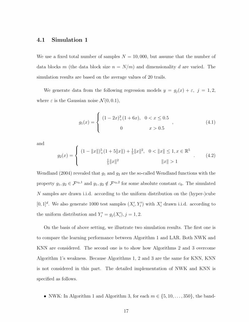
4.1 Simulation 1

We use a fixed total number of samples N = 10, 000, but assume that the number of

data blocks m (the data block size n = N/m) and dimensionality d are varied. The

simulation results are based on the average values of 20 trails.

We generate data from the following regression models y = gj(x) + ε, j = 1, 2,

where ε is the Gaussian noise N (0, 0.1),

g1(x) =

(1− 2x)3+(1 + 6x), 0 < x ≤ 0.5

0 x > 0.5, (4.1)

and

g2(x) =

(1− ‖x‖)5+(1 + 5‖x‖) + 15‖x‖2, 0 < ‖x‖ ≤ 1, x ∈ R5

15‖x‖2 ‖x‖ > 1

. (4.2)

Wendland (2004) revealed that g1 and g2 are the so-called Wendland functions with the

property g1, g2 ∈ F c0,1 and g1, g2 /∈ F c0,2 for some absolute constant c0. The simulated

N samples are drawn i.i.d. according to the uniform distribution on the (hyper-)cube

[0, 1]d. We also generate 1000 test samples (X ′i, Y′i ) with X ′i drawn i.i.d. according to

the uniform distribution and Y ′i = gj(X′i), j = 1, 2.

On the basis of above setting, we illustrate two simulation results. The first one is

to compare the learning performance between Algorithm 1 and LAR. Both NWK and

KNN are considered. The second one is to show how Algorithms 2 and 3 overcome

Algorithm 1’s weakness. Because Algorithms 1, 2 and 3 are the same for KNN, KNN

is not considered in this part. The detailed implementation of NWK and KNN is

specified as follows.

• NWK: In Algorithm 1 and Algorithm 3, for each m ∈ {5, 10, . . . , 350}, the band-

17

width parameter satisfies h ∼ N−1

2r+d according to Theorem 2 and Theorem 4. In

Algorithm 2, we set h ∼ max{m−1/(2r+d) maxj{hd/(2r+d)Dj},maxj{hDj}} according

to Theorem 3.

• KNN: According to Theorem 2, the parameter k is set to k ∼ N2r

2r+d

m. However,

as k ≥ 1, the range of m should satisfy m ∈ {1, 2, . . . , N2r

2r+d}.

To present proper constants for the localization parameters (e.g., h = cN−1

2r+d ), we

use the 5-fold cross-validation method in simulations. Based on these strategies, we

obtain the simulation results in the following Figures 1, 2 and 3.

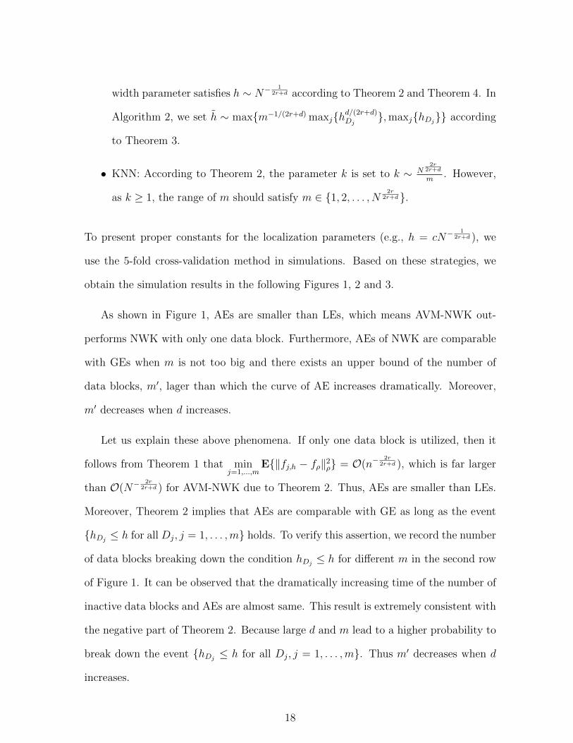
As shown in Figure 1, AEs are smaller than LEs, which means AVM-NWK out-

performs NWK with only one data block. Furthermore, AEs of NWK are comparable

with GEs when m is not too big and there exists an upper bound of the number of

data blocks, m′, lager than which the curve of AE increases dramatically. Moreover,

m′ decreases when d increases.

Let us explain these above phenomena. If only one data block is utilized, then it

follows from Theorem 1 that minj=1,...,m

E{‖fj,h − fρ‖2ρ} = O(n−2r

2r+d ), which is far larger

than O(N−2r

2r+d ) for AVM-NWK due to Theorem 2. Thus, AEs are smaller than LEs.

Moreover, Theorem 2 implies that AEs are comparable with GE as long as the event

{hDj ≤ h for all Dj, j = 1, . . . ,m} holds. To verify this assertion, we record the number

of data blocks breaking down the condition hDj ≤ h for different m in the second row

of Figure 1. It can be observed that the dramatically increasing time of the number of

inactive data blocks and AEs are almost same. This result is extremely consistent with

the negative part of Theorem 2. Because large d and m lead to a higher probability to

break down the event {hDj ≤ h for all Dj, j = 1, . . . ,m}. Thus m′ decreases when d

increases.

18

0 50 100 150 200 250 300 3500

0.5

1

1.5

2

2.5

3

3.5

4

4.5x 10−3

GEAELE

0 50 100 150 200 250 300 3500

10

20

30

40

50

60

70

80

0 50 100 150 200 250 300 3500

50

100

150

200

250

300

350

400

450

500

d = 1 d = 5

0 50 100 150 200 250 300 3500

1

2

3

4

5

6

7x 10−3

GEAELE

Figure 1: The first row shows AEs, LEs and GEs of NWK for different m. The secondrow shows the number of inactive machines which satisfy hDj > h. The vertical axisof the second row of Figure 1 is the number of inactive data blocks which break downthe condition hDj ≤ h.

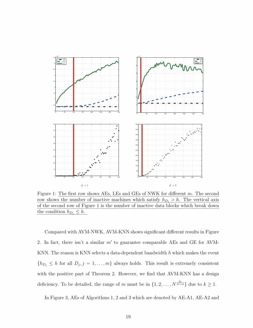
Compared with AVM-NWK, AVM-KNN shows significant different results in Figure

2. In fact, there isn’t a similar m′ to guarantee comparable AEs and GE for AVM-

KNN. The reason is KNN selects a data-dependent bandwidth h which makes the event

{hDj ≤ h for all Dj, j = 1, . . . ,m} always holds. This result is extremely consistent

with the positive part of Theorem 2. However, we find that AVM-KNN has a design

deficiency. To be detailed, the range of m must be in {1, 2, . . . , N2r

2r+d} due to k ≥ 1.

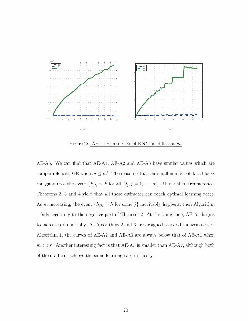
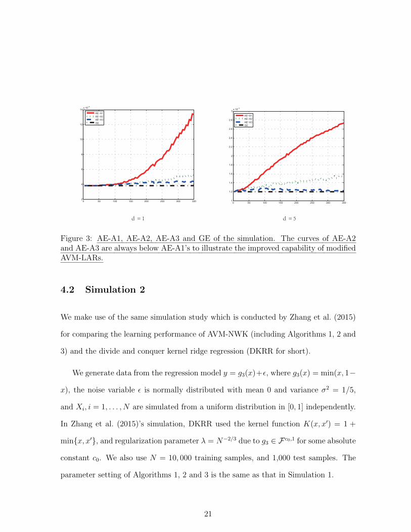
In Figure 3, AEs of Algorithms 1, 2 and 3 which are denoted by AE-A1, AE-A2 and

19

0 2 4 6 8 10 12 14 16 18 20 220.4

0.6

0.8

1

1.2

1.4

1.6

1.8x 10−3

GEAELE

0 10 20 30 40 50 60 701

2

3

4

5

6

7x 10−3

GEAELE

d = 1 d = 5

Figure 2: AEs, LEs and GEs of KNN for different m.

AE-A3. We can find that AE-A1, AE-A2 and AE-A3 have similar values which are

comparable with GE when m ≤ m′. The reason is that the small number of data blocks

can guarantee the event {hDj ≤ h for all Dj, j = 1, . . . ,m}. Under this circumstance,

Theorems 2, 3 and 4 yield that all these estimates can reach optimal learning rates.

As m increasing, the event {hDj > h for some j} inevitably happens, then Algorithm

1 fails according to the negative part of Theorem 2. At the same time, AE-A1 begins

to increase dramatically. As Algorithms 2 and 3 are designed to avoid the weakness of

Algorithm 1, the curves of AE-A2 and AE-A3 are always below that of AE-A1 when

m > m′. Another interesting fact is that AE-A3 is smaller than AE-A2, although both

of them all can achieve the same learning rate in theory.

20

0 50 100 150 200 250 300 3502

4

6

8

10

12

14x 10−4

AE−A1AE−A2AE−A3GE

0 50 100 150 200 250 300 3501

1.2

1.4

1.6

1.8

2

2.2

2.4

2.6

2.8

3x 10−3

AE−A1AE−A2AE−A3GE

d = 1 d = 5

Figure 3: AE-A1, AE-A2, AE-A3 and GE of the simulation. The curves of AE-A2and AE-A3 are always below AE-A1’s to illustrate the improved capability of modifiedAVM-LARs.

4.2 Simulation 2

We make use of the same simulation study which is conducted by Zhang et al. (2015)

for comparing the learning performance of AVM-NWK (including Algorithms 1, 2 and

3) and the divide and conquer kernel ridge regression (DKRR for short).

We generate data from the regression model y = g3(x)+ε, where g3(x) = min(x, 1−

x), the noise variable ε is normally distributed with mean 0 and variance σ2 = 1/5,

and Xi, i = 1, . . . , N are simulated from a uniform distribution in [0, 1] independently.

In Zhang et al. (2015)’s simulation, DKRR used the kernel function K(x, x′) = 1 +

min{x, x′}, and regularization parameter λ = N−2/3 due to g3 ∈ F c0,1 for some absolute

constant c0. We also use N = 10, 000 training samples, and 1,000 test samples. The

parameter setting of Algorithms 1, 2 and 3 is the same as that in Simulation 1.

21

101 102 1030

0.002

0.004

0.006

0.008

0.01

0.012

0.014AE−A1AE−A2AE−A3DKRR

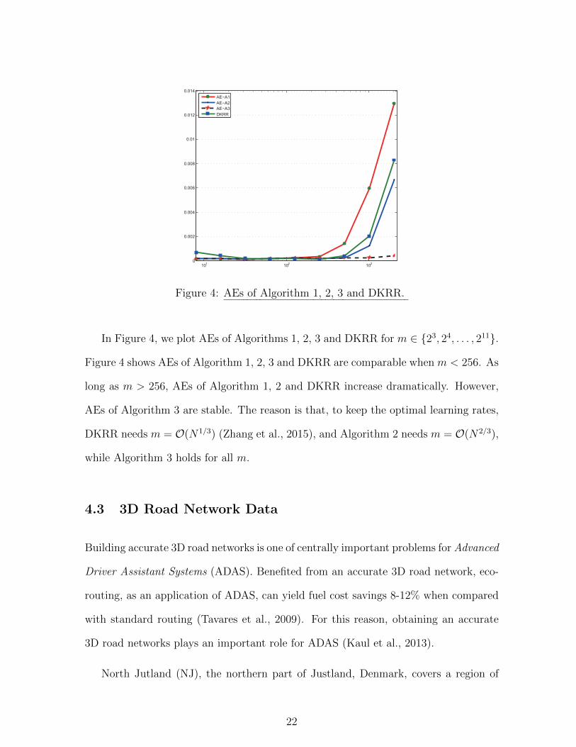
Figure 4: AEs of Algorithm 1, 2, 3 and DKRR.

In Figure 4, we plot AEs of Algorithms 1, 2, 3 and DKRR for m ∈ {23, 24, . . . , 211}.

Figure 4 shows AEs of Algorithm 1, 2, 3 and DKRR are comparable when m < 256. As

long as m > 256, AEs of Algorithm 1, 2 and DKRR increase dramatically. However,

AEs of Algorithm 3 are stable. The reason is that, to keep the optimal learning rates,

DKRR needs m = O(N1/3) (Zhang et al., 2015), and Algorithm 2 needs m = O(N2/3),

while Algorithm 3 holds for all m.

4.3 3D Road Network Data

Building accurate 3D road networks is one of centrally important problems for Advanced

Driver Assistant Systems (ADAS). Benefited from an accurate 3D road network, eco-

routing, as an application of ADAS, can yield fuel cost savings 8-12% when compared

with standard routing (Tavares et al., 2009). For this reason, obtaining an accurate

3D road networks plays an important role for ADAS (Kaul et al., 2013).

North Jutland (NJ), the northern part of Justland, Denmark, covers a region of

22

185km×130km. NJ contains a spatial road network with a total length of 1.17×107m,

whose 3D ployline representation is containing 414,363 points. Elevation values where

extracted from a publicly available massive Laser Scan Point Clod for Denmark are

added in the data set. Thus, the data set includes 4 attribute: OSMID which is the

OpenStreetMap ID for each road segment or edge in the graph; longitude and latitude

with Google format; elevation in meters. In practice, the acquired data set may include

missing values. In this subsection, we try to use AVM-LAR based on Algorithms 1,

2 and 3 for rebuilding the missing elevation information on the points of 3D road

networks via aerial laser scan data.

To this end, we randomly select 1000 samples as a test set (record time seed for

the reproducible research). Using the other samples, we run AVM-NWK based on

Algorithm 1, 2 and 3 to predict the missed elevation information in the test set. Here,

the bandwidth h = 0.13N−1/4 and N = 413, 363. AE-A1, AE-A2, AE-A3 and GE for

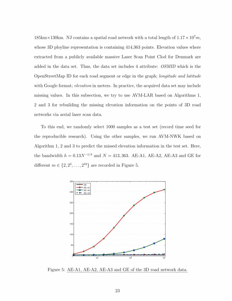
different m ∈ {2, 22, . . . , 210} are recorded in Figure 5.

101 102 1030

50

100

150

200

250

300

350

GEAE−A1AE−A2AE−A3

Figure 5: AE-A1, AE-A2, AE-A3 and GE of the 3D road network data.

23

We can find in Figure 5 that AEs of Algorithm 1 are larger than GE, which implies

the weakness of AVM-NWK based on the negative part of Theorem 2. AE-A3 has

almost same values with the GE for all m, however, AE-A2 possesses similar property

only when m ≤ 32. Then, for the 3D road network data set, Algorithm 3 is applicable

to fix the missed elevation information for the data set.

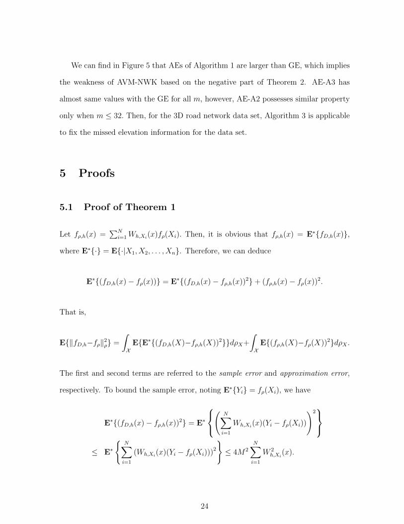
5 Proofs

5.1 Proof of Theorem 1

Let fρ,h(x) =∑N

i=1Wh,Xi(x)fρ(Xi). Then, it is obvious that fρ,h(x) = E∗{fD,h(x)},

where E∗{·} = E{·|X1, X2, . . . , Xn}. Therefore, we can deduce

E∗{(fD,h(x)− fρ(x))} = E∗{(fD,h(x)− fρ,h(x))2}+ (fρ,h(x)− fρ(x))2.

That is,

E{‖fD,h−fρ‖2ρ} =

∫X

E{E∗{(fD,h(X)−fρ,h(X))2}}dρX+

∫X

E{(fρ,h(X)−fρ(X))2}dρX .

The first and second terms are referred to the sample error and approximation error,

respectively. To bound the sample error, noting E∗{Yi} = fρ(Xi), we have

E∗{(fD,h(x)− fρ,h(x))2} = E∗

(

N∑i=1

Wh,Xi(x)(Yi − fρ(Xi))

)2

≤ E∗

{N∑i=1

(Wh,Xi(x)(Yi − fρ(Xi)))2

}≤ 4M2

N∑i=1

W 2h,Xi

(x).

24

Therefore we can use (A) to bound the sample error as

E{(fD,h(X)− fρ,h(X))2} ≤ 4M2E

{N∑i=1

W 2h,Xi

(X)

}≤ 4c1M

2

Nhd.

Now, we turn to bound the approximation error. Let Bh(x) be the l2 ball with center

x and radius h, we have

E{(fρ,h(X)− fρ(X))2} = E

(

N∑i=1

Wh,Xi(X)fρ(Xi)− fρ(X)

)2

= E

(

N∑i=1

Wh,Xi(X)(fρ(Xi)− fρ(X))

)2

= E

(

N∑i=1

Wh,Xi(X)(fρ(Xi)− fρ(X))

)2

I{Bh(X)∩D=∅}

+ E

(

N∑i=1

Wh,Xi(X)(fρ(Xi)− fρ(X))

)2

I{Bh(X)∩D 6=∅}

.

It follows from (Gyorfi et al., 2002, P.66) and∑N

i=1Wh,Xi(X) = 1 that

E

(

N∑i=1

Wh,Xi(X)(fρ(Xi)− fρ(X))

)2

I{Bh(X)∩D=∅}

≤ 16M2

Nhd.

25

Furthermore,

E

(

N∑i=1

Wh,Xi(X)(fρ(Xi)− fρ(X))

)2

I{Bh(X)∩D 6=∅}

≤ E

∑‖Xi−X‖≤h

Wh,Xi(X)|fρ(Xi)− fρ(X)|

2

I{Bh(X)∩D 6=∅}

+ E

∑‖Xi−X‖>h

Wh,Xi(X)|fρ(Xi)− fρ(X)|

2≤ c20h

2r +4c22M

2

Nhd,

where the last inequality is deduced by fρ ∈ F c0,r, condition (B) and Jensen’s inequal-

ity. Under this circumstance, we get

E{‖fD,h − fρ‖2ρ} ≤ c20h2r +

4(c1 + c22 + 4)M2

Nhd.

If we set h =(

4(c1+c22+4)M2

c20N

)−1/(2r+d), then

E{‖fD,h − fρ‖2ρ} ≤ c2d/(2r+d)0 (4(c1 + c22 + 4)M2)2r/(2r+d)N−2r/(2r+d).

This together with (Gyorfi et al., 2002, Theorem 3.2) finishes the proof of Theorem 1.

�

26

5.2 Proof of Theorem 2

Since E{‖fh − fρ‖2ρ

}= E

{‖fh − E{fh}+ E{fh} − fρ‖2ρ

}and E{fh} = E{fj,h}, j =

1, . . . ,m, we get

E{‖fh − fρ‖2ρ

}=

1

m2E

{m∑j=1

(‖fj,h − E{fj,h}‖2ρ + ‖E{fj,h} − fρ‖2ρ

)+ 2

m∑j=1

∑k 6=j

〈fj,h − E{fj,h}, fk,h − E{fk,h}〉ρ

}

=1

mE{‖f1,h − E{f1,h}‖2ρ}+ ‖E{f1,h} − fρ‖2ρ (5.1)

≤ 2

mE{‖f1,h − fρ}‖2ρ}+ 2‖E{f1,h} − fρ‖2ρ.

As h ≥ hDj for all 1 ≤ j ≤ m, we obtain that Bh(x) ∩ Dj 6= ∅ for all x ∈ X and

1 ≤ j ≤ m. Then, using the same method as that in the proof of Theorem 1, (C) and

(D∗) yield that

E{‖f1,h − fρ}‖2ρ} ≤ c20h2r +

4(c3 + c24)M2

nhd.

Due to the Jensen’s inequality, we have

E{‖fh − fρ‖2ρ

}≤ 2c20h

2r

m+

8(c3 + c24)M2

mnhd+ 2E

{‖E∗{f1,h} − fρ‖2ρ

}.

Noting Bh(X)∩Dj 6= ∅ almost surely, the same method as that in the proof of Theorem

1 together with (D) yields that

E{‖E∗{f1,h} − fρ‖2ρ

}≤ c20h

2r +8c24M

2

mnhd.

Thus,

E{‖fh − fρ‖2ρ

}≤ 16(c3 + c24)M

2

mnhd+ 3c20h

2r.

27

This finishes the proof of (2.6) by taking h =(

16(c3+c24)M2

3c20nm

)−1/(2r+d)into account.

Now, we turn to prove (2.7). According to (5.1), we have

E{‖fh − fρ‖2ρ

}≥ ‖E{f1,h} − fρ‖2ρ =

∫X

(E

{n∑i=1

WXi,h(X)fρ(Xi)− fρ(X)

})2

dρX .

Without loss of generality, we assume h < hD1 . It then follows from the definition of

the mesh norm that there exits X ∈ X which is not in Bh(Xi), Xi ∈ D1. Define the

separation radius of a set of points S = {ζi}ni=1 ⊂ X via

qS

:=1

2minj 6=k‖ζj − ζk‖.

The mesh ratio τS

:= hSqS≥ 1 provides a measure of how uniformly points in S are

distributed on X . If τS≤ 2, we then call S as the quasi-uniform point set. Let

Ξl = {ξ1, . . . , ξl} be l = b(2h)−dc quasi-uniform points (Wendland, 2004) in X . That

is τΞl

=h

Ξl

qΞl

≤ 2. Since hΞl≥ l−1/d, we have q

Ξl≥ 1

2l1/d≥ h. Then,

E{‖fh − fρ‖2ρ

}= ‖E{f1,h} − fρ‖2ρ

≥l∑

k=1

∫Bq

Ξl(ξk)

(E

{n∑i=1

WXi,h(X)fρ(Xi)− fρ(X)

})2

dρX .

If fρ(x) = M , then

E{‖fh − fρ‖2ρ

}≥ M2

l∑k=1

∫Bq

Ξl(ξk)

(E{I{D1∩BqΞl

(ξk)=∅}

})2dρX

≥ M2

l∑k=1

ρX(BqΞl

(ξk))P{D1 ∩BqΞl

(ξk) = ∅}

= M2

l∑k=1

ρX(BqΞl

(ξk))(1− ρX(BqΞl

(ξk)))n.

28

Since h ≥ 12(n+ 2)−1/d, we can let ρX be the marginal distribution satisfying

ρX(BqΞl

(ξk)) = 1/n, k = 1, 2, . . . , l − 1.

Then

E{‖fh − fρ‖2ρ

}≥M2

l−1∑k=1

1

n(1− 1/n)n ≥ M2((2h)−d − 2)

3n.

This finishes the proof of Theorem 2. �

5.3 Proof of Theorem 3

Without loss of generality, we assume hD1 = maxj{hDj}. It follows from (5.1) that

E{‖fh − fρ‖

2ρ

}≤ 2

mE{‖f1,h − fρ}‖

2ρ}+ 2‖E{f1,h} − fρ‖

2ρ.

We first bound E{‖f1,h − fρ}‖2ρ}. As h ≥ hD1 , the same method as that in the proof

of Theorem 2 yields that

E{‖f1,h − fρ}‖2ρ} ≤ c20E{h2r}+ E

{4M2(c3 + c24)

nhd

}.

To bound ‖E{f1,h}− fρ‖2ρ, we use the same method as that in the proof of Theorem 2

again. As h ≥ m−1/(2r+d)hd/(2r+d)D1

, it is easy to deduce that

‖E{f1,h} − fρ‖2ρ ≤ E

{‖E∗{f1,h} − fρ‖

2ρ

}≤ c20E{h2r}+ E

{8c24M

2

mnhd

}≤ c20m

−2r/(2r+d)E{h2rd/(2r+d)D1}+ c20E{h2rD1

}

+ 8c24M2(mn)−1E{md/(2r+d)h

−d2/(2r+d)D1

}.

29

Thus

E{‖fh − fρ}‖2ρ} ≤ c20m

−2r/(2r+d)E{h2rd/(2r+d)D1}+ (c20 + 2)E{h2rD1

}

+ 8(c3 + 2c24)M2(mn)−1md/(2r+d)E{h−d

2/(2r+d)D1

}.

To bound E{h2rd/(2r+d)D1}, we note that for arbitrary ε > 0, there holds

P{hD1 > ε} = P{maxx∈X

minXi∈D1

‖x−Xi‖ > ε} ≤ maxx∈X

E{(1− ρX(Bε(x)))n}.

Let t1, . . . , tl be the quasi-uniform points of X . Then it follows from (Gyorfi et al.,

2002, P.93) that P{hD1 > ε} ≤ 1nεd. Then, we have

E{h2rd/(2r+d)D1} =

∫ ∞0

P{h2rd/(2r+d)D1> ε}dε =

∫ ∞0

P{hD1 > ε(2r+d)/(2rd)}dε

≤∫ n−2r/(2r+d)

0

1dε+

∫ ∞n−2r/(2r+d)

P{hD1 > ε(2r+d)/(2rd)}dε

≤ n−2r/(2r+d) +1

n

∫ ∞n−2r/(2r+d)

ε−(2r+d)/(2r)dε ≤ 2r + d

dn−2r/(2r+d).

To bound E{h2rD1}, we can use the above method again and r < d/2 to derive E{h2rD1

} ≤

4rd−1n−2r/d. To bound E{h−d2/(2r+d)

D1}, we use the fact hD1 ≥ n−1/d almost surely to

obtain E{h−d2/(2r+d)

D1} ≤ nd/(2r+d). Hence

E{‖fh − fρ}‖2ρ} ≤

(c20(2r + d)

d+ 8(c3 + 2c24)M

2

)N−2r/(2r+d) +

4r(c20 + 2)

dn−2r/d.

Since

m ≤(c20(2r + d) + 8d(c3 + 2c24)M

2

4r(c20 + 2)

)d/(2r)N2r/(2r+d),

30

we have

E{‖fh − fρ}‖2ρ} ≤ 2

(c20(2r + d)

d+ 8(c3 + 2c24)M

2

)N−2r/(2r+d)

which finishes the proof of (3.2). �

5.4 Proof of Theorem 4

Proof. From the definition, it follows that

fh(x) =m∑j=1

I{Bh(x)∩Dj 6=∅}∑mj=1 I{Bh(x)∩Dj 6=∅}

∑(Xj

i ,Yji )∈Dj

Wh,Xji(x)Y j

i .

We then use Theorem 1 to consider a new local estimate with

W ∗h,Xj

i

(x) =I{Bh(x)∩Dj 6=∅}Wh,Xj

i(x)∑m

j=1 I{Bh(x)∩Dj 6=∅}.

We first prove (A) holds. To this end, we have

E

m∑j=1

∑(Xj

i ,Yji )∈Dj

(W ∗h,Xj

i

(X))2

≤ E

m∑j=1

∑(Xj

i ,Yji )∈Dj ,X

ji ∈Bh(X)

(W ∗h,Xj

i

(X))2

+ E

m∑j=1

∑(Xj

i ,Yji )∈Dj ,X

ji /∈Bh(X)

(W ∗h,Xj

i

(X))2

,

where we define∑

∅ = 0. To bound the first term in the right part of the above

inequality, it is easy to see that if I{Xji ∈Bh(X)} = 1, then I{Bh(X)∩Dj 6=∅} = 1, vice versa.

31

Thus, it follows from (C) that

E

m∑j=1

∑(Xj

i ,Yji )∈Dj ,X

ji ∈Bh(X)

(W ∗h,Xj

i

(X))2

=1

m2E

m∑j=1

∑(Xj

i ,Yji )∈Dj ,X

ji ∈Bh(X)

(Wh,Xji(X))2

≤ 1

mmax1≤j≤m

E

∑(Xj

i ,Yji )∈Dj ,X

ji ∈Bh(X)

(Wh,Xji(X))2

≤ 1

mmax1≤j≤m

E

∑(Xj

i ,Yji )∈Dj

(Wh,Xji(X))2

≤ c3

Nhd

To bound the second term, we have

E

m∑j=1

∑(Xj

i ,Yji )∈Dj ,X

ji /∈Bh(X)

(W ∗h,Xj

i

(X))2

= E

m∑j=1

∑(Xj

i ,Yji )∈Dj ,X

ji /∈Bh(X)

(I{Bh(X)∩Dj 6=∅}Wh,Xj

i(X)∑m

j=1 I{Bh(X)∩Dj 6=∅}

)2

At first, the same method as that in the proof of Theorem 1 yields that E{Bh(X)∩D =

∅} ≤ 4Nhd

. Therefore, we have

E

m∑j=1

∑(Xj

i ,Yji )∈Dj ,X

ji /∈Bh(X)

(I{Bh(X)∩Dj 6=∅}Wh,Xj

i(X)∑m

j=1 I{Bh(X)∩Dj 6=∅}

)2

≤ 4

Nhd+m max

1≤j≤mE

∑(Xj

i ,Yji )∈Dj

(Wh,Xj

i(X)I‖X−Xj

i ‖>h

)≤ 4 + c3 + c5

Nhd.

32

Now, we turn to prove (B) holds. This can be deduced directly by using the similar

method as the last inequality and the condition (E). That is,

E

m∑j=1

∑(Xj

i ,Yji )∈Dj

|W ∗h,Xj

i

(X)|I{‖X−Xi‖>h}

≤ c5√Nhd

.

Then Theorem 4 follows from Theorem 1. �

6 Conclusion

In this paper, we combined the divide and conquer strategy with local average regres-

sion to provide a new method called average-mixture local average regression (AVM-

LAR) to attack the massive data regression problems. We found that the estimate

obtained by AVM-LAR can achieve the minimax learning rate under a strict restric-

tion concerning m. We then proposed two variants of AVM-LAR to either lessen the

restriction or remove it. Theoretical analysis and simulation studies confirmed our

assertions.

We discuss here three interesting topics for future study. Firstly, LAR cannot

handle the high-dimensional data due to the curse of dimensionality (Gyorfi et al.,

2002; Fan, 2000). How to design variants of AVM-LAR to overcome this hurdle can be

accommodated as a desirable research topic. Secondly, we have justified that applying

the divide and conquer strategy on the LARs does not degenerate the order of learning

rate under mild conditions. However, we did not show there is no loss in the constant

factor. Discussing the constant factor of the optimal learning rate is an interesting

project. Finally, equipping other nonparametric methods (e.g., Fan and Gijbels (1994);

Gyorfi et al. (2002); Tsybakov (2008)) with the divide and conquer strategy can be

33

taken into consideration for massive data analysis. For example, Cheng and Shang

(2015) have discussed that how to appropriately apply the divide and conquer strategy

to the smoothing spline method.

References

Battey, H., Fan, J., Liu, H., Lu, J., and Zhu, Z. (2015), “Distributed Estimation and

Inference with Statistical Guarantees,” arXiv preprint arXiv:1509.05457.

Biau, G., Cadre, B., Rouviere, L., et al. (2010), “Statistical analysis of k-nearest neigh-

bor collaborative recommendation,” The Annals of Statistics, 38, 1568–1592.

Cheng, G. and Shang, Z. (2015), “Computational Limits of Divide-and-Conquer

Method,” arXiv preprint arXiv:1512.09226.

Dwork, C. and Smith, A. (2009), “Differential privacy for statistics: What we know

and what we want to learn,” Journal of Privacy and Confidentiality, 1, 135–154.

Fan, J. (2000), “Prospects of nonparametric modeling,” Journal of the American Sta-

tistical Association, 95, 1296–1300.

Fan, J. and Gijbels, I. (1994), “Censored regression: local linear approximations and

their applications,” Journal of the American Statistical Association, 89, 560–570.

Guha, S., Hafen, R., Rounds, J., Xia, J., Li, J., Xi, B., and Cleveland, W. S. (2012),

“Large complex data: divide and recombine (d&r) with rhipe,” Stat, 1, 53–67.

Gyorfi, L., Kohler, M., Krzyzak, A., and Walk, H. (2002), A distribution-free theory of

nonparametric regression, Springer Science & Business Media.

34

Kato, K. (2012), “Weighted Nadaraya–Watson estimation of conditional expected

shortfall,” Journal of Financial Econometrics, 10, 265–291.

Kaul, M., Yang, B., and Jensen, C. S. (2013), “Building accurate 3d spatial networks

to enable next generation intelligent transportation systems,” in Mobile Data Man-

agement (MDM), 2013 IEEE 14th International Conference on, IEEE, vol. 1, pp.

137–146.

Kramer, O., Satzger, B., and Lassig, J. (2010), “Power prediction in smart grids

with evolutionary local kernel regression,” in Hybrid Artificial Intelligence Systems,

Springer, pp. 262–269.

Li, R., Lin, D. K., and Li, B. (2013), “Statistical inference in massive data sets,”

Applied Stochastic Models in Business and Industry, 29, 399–409.

Mcdonald, R., Mohri, M., Silberman, N., Walker, D., and Mann, G. S. (2009), “Ef-

ficient large-scale distributed training of conditional maximum entropy models,” in

Advances in Neural Information Processing Systems, pp. 1231–1239.

Stone, C. J. (1977), “Consistent nonparametric regression,” The annals of statistics,

595–620.

— (1980), “Optimal rates of convergence for nonparametric estimators,” The annals

of Statistics, 1348–1360.

— (1982), “Optimal global rates of convergence for nonparametric regression,” The

annals of statistics, 1040–1053.

Takeda, H., Farsiu, S., and Milanfar, P. (2007), “Kernel regression for image processing

and reconstruction,” Image Processing, IEEE Transactions on, 16, 349–366.

35

Tavares, G., Zsigraiova, Z., Semiao, V., and Carvalho, M. d. G. (2009), “Optimisation

of MSW collection routes for minimum fuel consumption using 3D GIS modelling,”

Waste Management, 29, 1176–1185.

Tsybakov, A. B. (2008), Introduction to nonparametric estimation, Springer Science &

Business Media.

Wang, C., Chen, M.-H., Schifano, E., Wu, J., and Yan, J. (2015), “Statistical Methods

and Computing for Big Data,” arXiv preprint arXiv:1502.07989.

Wendland, H. (2004), Scattered data approximation, vol. 17, Cambridge university

press.

Wu, X., Zhu, X., Wu, G.-Q., and Ding, W. (2014), “Data mining with big data,”

Knowledge and Data Engineering, IEEE Transactions on, 26, 97–107.

Zhang, Y., Duchi, J. C., and Wainwright, M. J. (2015), “Divide and conquer kernel

ridge regression: A distributed algorithm with minimax optimal rates,” Journal of

Machine Learning Research, to appear.

Zhang, Y., Wainwright, M. J., and Duchi, J. C. (2013), “Communication-efficient

algorithms for statistical optimization,” Journal of Machine Learning Research, 14,

3321–3363.

Zhou, Z., Chawla, N., Jin, Y., and Williams, G. (2014), “Big Data Opportunities

and Challenges: Discussions from Data Analytics Perspectives [Discussion Forum],”

Computational Intelligence Magazine, IEEE, 9, 62–74.

36