Diversification strategies and scope economies: · PDF fileGuido Del Mese (ASSTRA) ......
34
Diversification strategies and scope economies: Evidence from a sample of Italian regional bus transportation providers Elisabetta OTTOZ, Marina DI GIACOMO Working Paper 7, anno 2007
Transcript of Diversification strategies and scope economies: · PDF fileGuido Del Mese (ASSTRA) ......

Diversification strategies and scope economies: Evidence from a sample of Italian regional bus
transportation providers
Elisabetta OTTOZ, Marina DI GIACOMO
Working Paper 7, anno 2007

© HERMES Fondazione Collegio Carlo Alberto Via Real Collegio, 30 10024 - Moncalieri (TO) Tel: 011 670 5250 Fax: 011 6705089 [email protected] http://www.hermesricerche.it I diritti di riproduzione, di memorizzazione e di adattamento totale o parziale con qualsiasi mezzo (compresi microfilm e copie fotostatiche) sono riservati. PRESIDENTE Giovanni Fraquelli SEGRETARIO Cristina Piai COMITATO DIRETTIVO Giovanni Fraquelli (Presidente) Cristina Piai (Segretario) Guido Del Mese (ASSTRA) Carla Ferrari (Compagnia di San Paolo) Giancarlo Guiati (GTT S.p.A.) Mario Rey (Università di Torino) COMITATO SCIENTIFICO Tiziano Treu (Presidente, Università "Cattolica del Sacro Cuore" di Milano e Senato della Repubblica) Giuseppe Caia (Università di Bologna) Roberto Cavallo Perin (Università di Torino) Giovanni Corona (CTM S.p.A.) Graziella Fornengo (Università di Torino) Giovanni Fraquelli (Università del Piemonte Orientale "A. Avogadro") Carlo Emanuele Gallo (Università di Torino) Giovanni Guerra (Politecnico di Torino) Marc Ivaldi (IDEI, Universitè des Sciences Sociales de Toulouse) Carla Marchese (Università del Piemonte Orientale "A. Avogadro") Luigi Prosperetti (Università di Milano "Bicocca") Alberto Romano (Università di Roma "La Sapienza") Paolo Tesauro (Università di Napoli "Federico" II)

3
Diversification strategies and scope economies: Evidence from a sample of Italian regional bus transportation providers
Elisabetta Ottoz* Marina Di Giacomo**
University of Turin University of Turin Hermes Research Centre
December 2007
Abstract
A growing number of local public transportation (LPT) companies diversify their production lines by providing a large set of services. In particular different strategies are observed depending on the ownership structure: while private firms mainly supply competitive markets, usually highly correlated to the core business (e.g. bus renting and coaching activities), publicly owned companies (mainly municipal firms) offer a very large set of products in regulated sectors, ranging from car park management to waste disposal, water and sewage treatment and gas and electricity distribution. The cost properties of a sample of LPT companies operating in Piedmont, a Northern Italy region, are investigated and the presence and the magnitude of scope economies are assessed. The results from different functional forms are compared and estimates point towards the presence of global economies of scope. Scope economies for the median firm range between 16% and 30% depending on the output definition and the chosen cost function. Public firms always show lower scope economies. Global density economies are also detected, but they disappear when product specific density economies are considered. The general picture seems to be characterized by local public transport firms that enjoy global scope economies, that are particularly high for private firms, i.e. for small to medium sized firms that diversify in competitive industries. Public firms are characterized by lower scope economies, and sometimes diseconomies, both because of their larger size and because of their chosen production structure. Keywords: cost function, scope economies, transport companies JEL: C33, L25, L33, L92
* Università degli Studi di Torino, Dipartimento di Economia,Via Po 53, 10124, Torino, Italy. Tel. +39(0)11-670 2739. Email: [email protected]
**Università degli Studi di Torino, Facoltà di Economia, Corso Unione Sovietica 218bis, 10134 Torino, Italy. Tel: +39(0)11-670 6186. E-mail: [email protected]; HERMES: Higher Education and Research on Mobility Regulation and the Economics of Local Services, Collegio Carlo Alberto, via Real Collegio 30, 10024 Moncalieri (TO).
Acknowledgements: We wish to thank Graziella Fornengo for fruitful discussions and Luca Sanlorenzo for outstanding assistance on the data. Financial support from Hermes (Higher Education and Research on Mobility Regulation and the Economics of Local Services) Research Centre is gratefully acknowledged. All errors are our own.

4
1. Introduction
Only few papers analysed scope economies in the local public transport (LPT)
industry where a growing number of companies diversify their production lines by
providing a large set of services.
This study tries to fill this gap using data from a sample of Italian bus companies
observed over the period 1998-2004, that diversify their core activities supplying also
transport related services and / or non transport services.
The sample of firms is also characterized by different ownership structures that are
coupled with different diversification strategies. Private firms mainly supply services
that are highly related to the core business (e.g. bus renting and coaching activities),
while publicly owned companies (mainly municipal firms) offer a very large set of
products, ranging from car park management to waste disposal, water and sewage
treatment and gas and electricity distribution. In particular, while private firms mainly
diversify in competitive markets, public companies are usually active in regulated
sectors. The analysis aims to better understand the economic justification for such
managerial choices and the presence of actual cost savings from the diversification in
competitive versus regulated markets.
Our strategy is to estimate a cost function, using different model specifications. Many
authors indicated the unreliable results from the standard translog specification when
the main object is the analysis of scope economies and cost complementarities.
Findings from the generalized (Box-Cox) translog function model are compared to
those from the composite cost function introduced by Pulley and Braunstein (1992)
that appear to be more suitable for studying the cost properties of multi- product firms.
Next section briefly reviews the main literature on scope economies in the bus
transport industry and on functional choice for a cost model. Section 3 gives details on
the different cost specifications that are estimated, while section 4 describes the
dataset. Section 5 presents the main estimation results and a discussion on the
economies of scope and size is given in section 6. Section 7 concludes and the
appendix contains the tables showing the full set of estimation results.

5
2. Literature review
A scant number of papers consider scope economies in the public transit industry.
Viton (1992) considers urban transit companies supplying their services in six modes
(motor bus, street cars, rapid rail, etc.) and the presence of scope and scale economies
is uncovered. Similarly Colburn and Talley (1992) analyze a four modes urban
company and find only limited cost complementarities. Viton (1993) estimates a
quadratic cost frontier for bus companies operating in the San Francisco bay area and
he is able to evaluate the cost savings deriving from the merger of the seven
companies in the sample. Cost savings depend on the modes being offered and on the
number of merging firms, with benefits decreasing as the number of integrated
companies increases.
Farsi et al. (2007) study a sample of Swiss companies supplying urban services using
three modes: trolley bus, motor bus and tramway systems. They detect global scope
economies for multi-modal operators from the estimation of a quadratic cost function.
Many studies have considered the issue of the choice of the functional form for a cost
model when the main purpose is to quantify the existence of scope economies from
the simultaneous provision of different outputs. In general there seems to be a trade
off among flexible functional forms that satisfy all regularity conditions that are
required for a cost function to be an adequate representation of the production
technology (concavity in input prices, non decreasing in input prices and outputs) and
the dimension of the region over which such regularity conditions are fulfilled. Roller
(1990) emphasizes that “this ‘regular’ region may be too small to be able to model
demanding cost concepts such as economies of scope and subadditivity”. The most
popular flexible functional forms, such as the standard translog model (see
Christensen et al., 1971), have a degenerate behaviour in the region which is relevant
for the derivation of scope economies and subadditivity measures (in general zero
outputs levels) even if they satisfy the regularity conditions for a larger set of points
(see Diewert, 1974 and Diewert and Wales, 1987).
Pulley and Braunstein (1992) and Pulley and Humphrey (1993) introduce the
composite specification that unlike the translog models is defined in the
neighbourhood of zero output levels and allows for the estimation of scope
economies. McKillop et al. (1996), McKenzie and Small (1997), Bloch et al. (2001),

6
Fraquelli et al. (2004), Piacenza and Vannoni (2004) and Fraquelli et al. (2005) all
adopted the composite specification as their preferred model for the derivation of
scope economies in different industries (ranging from the banking sector to the public
utilities).
3. The cost function model
Our aim is to study the cost structure of a sample of transportation companies
operating in the administrative region of Piedmont, in Northern Italy. In particular we
are going to estimate a multi output cost function since firms may provide a large set
of services.
A stochastic cost function can be written as:
ftfftftft uCC ++= νθ );,( py
where Cit is total cost for firm f =1,…,F, at time t=1,…T, yft is the vector of outputs for
firm f at time t, pft is the vector of input prices, θ is the vector of unknown parameters
to be estimated, νf is the firm specific time invariant error term, while uft is the
remainder stochastic error term that varies over time and across companies. Given the
panel structure of the data, we are going to assume the absence of correlation among
the individual specific effects νf and the included regressors, i.e.
0),|( =ftftfE pyν . This assumption allows for the consistency of the pooled
nonlinear estimation procedure while panel robust standard errors that take into
account the likely correlation among errors for the same individuals should ensure
robust inference. When dealing with nonlinear functional forms, the estimation of
fixed effects or random effects models, as for linear specifications, is not
straightforward (see Cameron and Trivedi, 2005, chapter 23 for a survey) and
solutions are mainly case specific. At the same time including a large set of firm
specific dummy variables may lead to inconsistent estimates as the incidental problem
arises (see Lancaster, 2000). Our choice of a pooled model is justified by the lower
computational burden and the unreliable estimates that were obtained when trying to
estimate a model where all individual dummy variables are included.
We are going to present results from a two outputs and a three outputs cost models,
that mainly differ in the way the considered outputs are aggregated (see Pulley and

7
Humphrey, 1993, for a similar approach when studying scope economies in the
banking sector). Section 4 gives details on the dataset construction.
We are also going to compare results from different cost specifications. Baumol et al.
(1982) recommend a quadratic output structure when examining scope economies
because this form allows for the direct handling of zero outputs, without any need for
substitutions or transformations as in the translog models. We thus estimate a
composite and a separable quadratic cost specification that have a quadratic structure
in outputs and a log – quadratic structure in input prices, but also a standard translog
and a generalized translog model.
The composite specification that we consider has the following form (see Carroll and
Rupert, 1984, 1988 and Pulley and Braunstein, 1992 for more details):
)()],(ln[lnln21ln
ln21ln)ln( 2
210
ppy fhppβpβ
TrendTrendpyyyyC
r r qqrrqrr
i rriir
i jijij
iii
+=⎥⎥⎦
⎤
⎢⎢⎣
⎡+
+⎟⎟
⎠
⎞
⎜⎜
⎝
⎛+++++=
∑ ∑∑
∑∑∑∑∑ λλαααα
(1)
where C is the total cost, yi is output i, i= T, TR, NT, for transport, transport related
and non transport services respectively; pr is price for input r=L, M, K, for labour,
material and capital respectively and Trend - Trend2 are a linear and a quadratic time
trend respectively.
By applying the Shephard’s Lemma, the associated input share equation is:
⋅⎟⎟
⎠
⎞
⎜⎜
⎝
⎛+++++
⋅⎟⎟⎠
⎞⎜⎜⎝
⎛+
⎥⎥⎦
⎤
⎢⎢⎣
⎡+=
∂∂
==
−
∑∑∑∑∑
∑∑1
2210 ln
21
lnln
)ln(
TrendTrendpyyyy
ypββpC
CpxS
i rriir
i jijij
iii
iiir
qqrqr
r
rrr
λλαααα
α
where xr is the derived demand for input r (xr=∂C/∂pr).
The separable quadratic model only differs from the composite specification in the
assumed restriction that αir = 0 for all i and r.
The generalized translog function is:
8
221,
)()()()(0
lnln21ln
ln21)ln(
TrendTrendppβpβ
pyyyyC
qrrqqrrrr
i rriir
i i jjiijii
λλ
αααα ππππ
+++
++++=
∑∑
∑∑∑ ∑∑ (2)
where yi(π) is the Box – Cox (1964) transformation of the output measure i:
0)ln(
0/)1()(
==
≠−=
π
ππππ
ify
ifyy
i
i i
The standard translog specification follows from the imposition of the restriction π =
0 in equation (2).
The input share equation associated to the generalized translog specification is:
∑∑ ++=∂∂
==q
qrqri
irr
rrr pββy
pC
CpxS
iln
ln)ln( )(πα
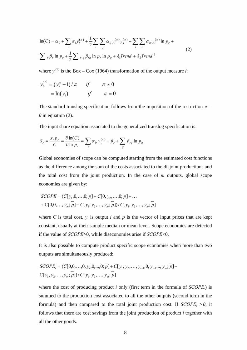
Global economies of scope can be computed starting from the estimated cost functions
as the difference among the sum of the costs associated to the disjoint productions and
the total cost from the joint production. In the case of m outputs, global scope
economies are given by:
];,,,[/]);,,,[];,,0,0[
];0,,,0[];0,,0,[(
2121
21
pyyyCpyyyCpyC
pyCpyCSCOPE
mmm KKK
KKK
−+
++=
where C is total cost, yi is output i and p is the vector of input prices that are kept
constant, usually at their sample median or mean level. Scope economies are detected
if the value of SCOPE>0, while diseconomies arise if SCOPE<0.
It is also possible to compute product specific scope economies when more than two
outputs are simultaneously produced:
];,,,[/]);,,,[
];...,,0,,,,[];0,...,0,,0,,0,0[(
2121
1121
pyyyCpyyyC
pyyyyyCpyCSCOPE
mm
miiii
KK
KK −+= +−
where the cost of producing product i only (first term in the formula of SCOPEi) is
summed to the production cost associated to all the other outputs (second term in the
formula) and then compared to the total joint production cost. If SCOPEi >0, it
follows that there are cost savings from the joint production of product i together with
all the other goods.

9
Finally we can calculate scope economies for different pairs of products:
];0,...,0,,0,...,0,,0,,0,0[/]);0,...,0,,0,...,0,,0,,0,0[
];0,...,0,,0,,0,0[];0,...,0,,0,,0,0[(
pyyCpyyC
pyCpyCSCOPE
jiji
jiij
KK
KK −+=
for products i and j, with i≠j, SCOPEij>0 indicates the presence of scope economies
from the joint production of the two goods, given the estimated cost structure.
Following Pulley and Humphrey (1993) we are also going to distinguish among the
sources of cost savings. Using the composite (and separable quadratic) specification it
is possible to distinguish among the fixed costs and variable costs savings, once scope
economies are assessed. Given the formula in (1) for the composite cost function, it
follows that global scope economies are given by:
( )),(
)1(,
pyh
yymSCOPE iji jiijo ∑ ≠
−−=
αα
where the portion of scope economies that can be ascribed to fixed costs savings, i.e. a
reduction in excess capacity that allows for the spreading of fixed costs over a larger
production set, is given by:
( )),(
)1(pyh
mSCOPE oFixedCost
α−= (3)
and scope economies attributable to savings from cost complementarities, i.e. savings
associated to variable inputs that can be shared by different production lines, equal:
),(,
pyh
yySCOPE iji jiij
CostComplement
⎟⎠⎞⎜
⎝⎛−
=∑ ≠
α
The estimated fixed costs savings in (3) represent an upper – bound estimate of the
true effects from spreading fixed costs over a larger set of outputs. In fact as Pulley
and Humphrey (1993) highlight, we are not able to identify product specific fixed
costs and we use the estimated fixed costs from joint production (the constant term α0
in the composite specification, see equation (3)) as a proxy for fixed costs of
producing each output separately. The correct formula of the fixed cost savings, e.g.
for a three outputs cost function (i=1, 2, 3), is:

10
( )
),(3,2,1;03;02;01;0
pyhSCOPE FixedCost
αααα −++=
where α0;1 is a measure of fixed costs associated to the first output that can be
estimated as the coefficient of a dummy variable that takes the value of one for
companies that produce only output 1 and zero otherwise. Similarly α0;2 and α0;3 can
be estimated as intercepts specific to outputs 2 and 3 respectively, while α0;1,2,3 is the
estimated fixed cost for joint production. Identification of the different components of
the correct formula is feasible when data on specialized firms are available.
Unfortunately this is rarely the case and in our dataset we do not observe any
specialized companies.
Size economies are also evaluated. As pointed out by Caves et al. (1984) when dealing
with industries where network represents an important attribute of the production, it
should be considered the difference among density and scale economies. While
density economies consider how the average costs change when output increases,
keeping the network dimension fixed, in the computation of scale economies the
enhancement of both outputs and network size are taken into account. We are not
going to consider any network measure in the estimation of the cost function, thus we
are able to evaluate the magnitude of global density economies (DENSITY) and
product specific density economies (DENSITYi) respectively:
1
)ln()ln(
−
⎟⎟⎠
⎞⎜⎜⎝
⎛∂∂
= ∑i iy
CDENSITY
where the derivatives need to be interpreted as cost elasticities with respect to the ith
output;
i
imiimi
yC
ypyyyyyCpyyyCDENSITY
∂∂
−= +− /));,...,,0,,,,();,,,(( 112121 KK
where the numerator is the average incremental cost (AIC), i.e. the additional costs of
increasing product i from zero to yi, holding all other outputs (and the input prices)
fixed; while the denominator is the marginal cost with respect to product i.

11
Economies of density are present when DENSITY is greater than one, while
diseconomies of density are present if DENSITY is smaller than one. Neither
economies nor diseconomies exist if DENSITY is equal to one.
Finally the effect of technical change on total costs is computed. The inclusion of a
linear and a quadratic time trend in all specifications should proxy for technical
change. Technical progress is detected if 0)ln( >∂∂− TrendC , while technical
regress follows if the derivative is smaller than zero.
4. Industry and data description
Data come from two sources: the database owned by the administrative region of
Piedmont, which yearly collects information on transport services supplied by the
companies of the area and the official accounting reports of the firms.
The regional database reports data on total costs, input costs and outputs for all the
companies supplying local public transportation services. We complement these data,
providing information on transport activities only, with companies’ financial
statements. The aim is to obtain a comprehensive picture of the whole set of services
and outputs that transport companies offer.
Our final sample is an unbalanced panel of 40 firms whose annual observations cover
the period 1998-2004.
We define three broad outputs: subsidized local public transportation services, non
subsidized transport related activities and non transport services.
Local public transportation comprises urban and intercity transport connections that
represent the main business for all the firms in our sample. Non subsidized transport
related activities may range from coach renting to touristic travel organization.
Non transport services mainly relate to regulated markets and they represent a broad
and varied set of productions such as waste disposal, water and sewage treatment,
parking areas management, cemetery services and gas and electricity distribution.
Information on such services come from the companies’ financial statements.
We use total revenues from each of the three production sets as our output measures in
the estimation of the cost function. The prices for transport outputs and for other
transport related activities are approximated by the consumer price indexes for

12
transport services while we use the consumer price index for housing, water,
electricity and fuels as a proxy for non transport outputs’ price. The output quantities
for transport services (yT) are thus computed as the transport revenues divided by the
price index of transport facilities. The output quantities for transport related activities
(yTR) are calculated dividing total revenues from these services by the price index for
transportation, while the outputs for the other non transport productions (yNT) are
obtained dividing total revenues associated to such products by the consumer price
index for housing, water, electricity and fuels. Estimation results from a two outputs
technology are also reported. In this case subsidized local public transportation
services (yT as defined above) are contrasted to non subsidized activities, given by the
sum of total revenues from transport related services and all the other services. The
consumer price index for transportation and the consumer price index for housing,
water, electricity and fuels are used as proxies for output prices for the two production
sets respectively.
The choice of such values as our outputs was mainly motivated by measurement
difficulties. Many outputs definition have been adopted in transport studies, usually
grouped into demand oriented measures (such as passengers-kilometres) and supply
oriented outputs (like vehicle- kilometres or seat- kilometres). More ambiguous is the
definition of a measure for the other two outputs. Transport related activities could in
principle be measured by vehicle – kilometres or seat – kilometres as for transport
services, however such values are not available for all companies in our sample. Even
more demanding is the task for other non transport services as they are a very
heterogeneous category (car parks management, electricity and gas distribution, water
and sewage treatment, waste disposal, etc.), and we were not able to disentangle the
information on each single activity. Total revenues were finally selected as they were
readily available while index prices should control for price effects. A similar
approach was followed, among the others, by McKillop et al. (1996) in their study of
giant Japanese banks, Cowie and Asenova (1999) for the assessment of cost
inefficiencies in the British bus industry, Silk and Berndt (2004) for marketing firms
and Asai (2006) for the broadcasting industry.
Total costs for a firm are given by the total production costs as they are reported by
the annual company profit and loss accounts.
Three inputs are considered: labour, materials and capital.

13
Labour price (pL) is calculated dividing total labour costs as they appear in the profit
and loss account, by the total number of employees of the company. Labour cost share
is computed dividing total labour costs by total costs.
Total material costs are obtained from the corresponding company account item and
include raw materials, consumption and maintenance goods’ purchases, energy and
fuel expenses. The price for this heterogeneous input is measured by the production
price index for energy and gas, since most of the expenditures for materials were for
energy and fuels. The cost share for materials is given by the ratio of total material
costs to total production costs.
Following Christensen and Jorgenson (1969), price for capital (pK) is computed by
PPI(IR+D)/(1-T), where PPI is the production price index for investment goods, IR is
the yearly average long term prime lending interest rate as assessed by the Italian
Banking Association (ABI1), while D is the depreciation rate and T is the corporate
tax rate.
D is computed as the ratio of total depreciation expenses to book-valued fixed assets
at the beginning of the period. T is obtained as total taxation divided by operating
profits taken from the financial statements. A similar approach for the derivation of
capital and material prices is followed by Adams et al. (2004) and Asai (2006).
Data on yearly consumption price indexes (for transportation and for housing, energy
and fuels) and production price indexes (for energy and for investments goods) are
obtained from ISTAT, Italian Statistical Institute2. The consumption price indexes are
town (province) specific and we apply the appropriate price index according to the
town (province) where the company runs its businesses.
Tables 1 and 2 report some descriptive statistics for the sample.
Firms are quite heterogeneous in their operating size: standard deviations for total
operating costs and total revenues are quite high and the median is always smaller
than the mean. Companies are asymmetrically distributed and few very large firms
share the market with many small – medium sized LPT firms. The largest firms in the
sample are publicly owned and table 2 splits the sample according to ownership. Apart
1 Data available from the Bank of Italy website, www.bancaditalia.it 2 Data available from www.istat.it

14
from the size differences3, it is interesting to note the different production lines for the
two groups of firms considering the median output levels: while publicly owned firms,
mainly municipal entities, are diversified in regulated markets, such as e.g. waste
disposal, water and sewage treatment and gas and electricity distribution; private
companies diversify their activities in competitive unregulated sectors, like transport
related services, such as bus renting, coaching activities and touristic services.
Differences across the firms in the sample and between public and private companies
are less evident when we look at the inputs: labour and capital prices as well as labour
and material costs shares on total costs are characterized by small standard deviations.
Table 1. Descriptive statistics for the whole sample. Unbalanced panel: 40 firms over the
period 1998-2004, 184 observations.
Mean Std. Dev. Median Total operating costs (th. Euro) 8958.98 33294.42 3416.91Total revenues from transport services (th. Euro) 3990.99 9732.31 1717.06Total revenues from non transport services (th. Euro) 2282.80 6821.18 101.02Total revenues from transport related services (th. Euro) 3017.14 19798.13 604.86yT 36.34 83.85 16.10yNT 20.21 58.65 0.95yTR 26.43 168.61 5.48Labour price pL (th. Euro) 35.68 32.65 33.86Material price pM (price index) 119.70 12.84 124.10Capital price pK 34.40 20.90 28.02Labour share 0.45 0.10 0.44Material share 0.18 0.08 0.17Total cost of personnel (th. Euro) 4423.29 17786.84 1436.71Number of employees 134.44 539.38 40.50Total cost of materials (th. Euro) 1421.05 3690.66 626.81Notes: See the text for the definition of the output measures yT , yNT, , yTR and the capital price pK,.
3 The largest firm in the dataset is GTT (Gruppo Torinese Trasporti), owned by the municipality of Turin.

15
Table 2. Descriptive statistics for the samples of publicly and privately owned companies.
11 public firms, 49 obs. 29 private firms, 135 obs. Mean Std. dev. Median Mean Std. dev. Median Total operating costs (th. Euro) 22725.86 62704.37 10013.16 3962.12 3315.54 2422.29Total revenues from transport services (th. Euro) 7505.56 17820.75 2902.14 2715.34 3072.04 1635.00
Total revenues from non transport services (th. Euro) 7674.42 11640.51 1583.73 325.84 718.80 48.25
Total revenues from transport related services (th. Euro) 8152.90 38131.81 88.90 1153.04 1141.38 770.32
yT 66.75 152.37 24.97 25.30 28.72 15.85yNT 67.43 99.38 13.65 3.07 6.95 0.47yTR 69.79 324.74 0.81 10.69 10.48 7.19Labour price pL (th. Euro) 42.49 61.69 33.93 33.21 8.31 33.75Material price pM (price index) 123.38 9.92 124.30 118.36 13.53 124.10Capital price pK 30.05 23.42 26.18 35.98 19.77 29.19
Notes: See the text for the definition of the output measures yT , yNT, , yTR and the capital price pK,.
Before estimation all variables, except for the linear and the quadratic time trends
(Trend and Trend2) that should capture technical change, are normalised by their
sample median levels. Moreover in order to cope with the required regularity
conditions for cost functions, a number of restrictions are imposed in all models.
Symmetry is ensured by the imposition of the following equalities in all cost
specifications (see equations (1) and (2)): αij = αji and βrk = βkr. Linear homogeneity,
requiring Σrαir =0 for all i; Σrβr=1 and Σkβrk=0 for all k, is obtained dividing both the
dependent variable (total costs) and the labour and material prices by the capital price
which does not directly appear in the estimated function. The other regularity
conditions (nonnegative marginal costs with respect to outputs, non decreasing costs
in input prices and concavity of the cost function in input prices) are checked after
estimation for all sample observations.
5. Estimation results
Table 3 presents the estimated parameters for the cost functions that use the two most
general specifications: the generalized translog and the composite forms. Results for
the two outputs and the three outputs models are shown. The appendix reports the
estimation results for the four specifications that are described in section 3 (that
include also the standard translog and the separable quadratic models).

16
The estimated parameters greatly differ according to the definition of outputs. The
considered three outputs are transport, transport related and non transport services,
while in the specification with two outputs, non transport services are defined as the
sum of transport related and all the other non transport activities.
The first order terms for outputs are positive and statistically significant in all
specifications. The second order and the interaction coefficients for outputs are never
significant for the composite model (except for the interaction among transport and
transport related services), while they are precisely estimated under the generalized
translog model. The second order output coefficients are not particularly large (when
compared to the first order coefficients) and, as Bloch et al. (2001) suggest, this
produces reliable scale and scope economies since output cost elasticities are more
stable4.
First order parameters for the labour price are always precisely estimated and differ
across specifications, with larger magnitudes from the composite models. The
coefficients for material prices are significant only under the first specification
(generalized translog with two outputs) and are much smaller than those for labour
price, paralleling the different median cost shares (labour costs represent 45% of total
operating costs, while material costs correspond to 18%).
The time trend parameter is negative and significant in all specifications, indicating
cost reductions over time. The positive second order trend coefficients, however,
indicates that such cost savings diminish over time.
4 Large second order output coefficients imply that a marginal increase in an output causes a large change in cost elasticity. This happens, for example, with the standard translog model (see table 1A and 2A in the appendix) where the second order coefficient for transport services is quite large, resulting in implausible transport specific density returns estimates.
17
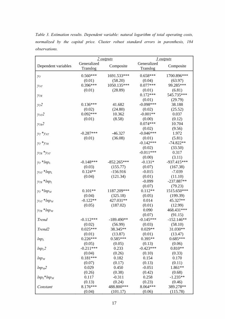
Table 3. Estimation results. Dependent variable: natural logarithm of total operating costs,
normalized by the capital price. Cluster robust standard errors in parenthesis, 184
observations.
2 outputs 3 outputs
Dependent variables Generalized Translog Composite Generalized
Translog Composite
yT 0.560*** 1691.533*** 0.658*** 1700.896*** (0.01) (58.20) (0.04) (63.97) yNT 0.396*** 1050.135*** 0.077*** 99.285*** (0.01) (28.89) (0.01) (6.81) yTR 0.172*** 545.735*** (0.01) (29.79) yT2 0.136*** 41.682 -0.098*** 38.188 (0.02) (24.80) (0.02) (25.52) yNT2 0.092*** 10.362 -0.001** 0.037 (0.01) (8.58) (0.00) (0.12) yTR2 0.074*** 10.704 (0.02) (9.56) yT *yNT -0.287*** -46.327 -0.046*** 1.972 (0.01) (36.08) (0.01) (5.81) yT *yTR -0.142*** -74.822** (0.02) (33.50) yTR *yNT -0.011*** 0.317 (0.00) (3.11) yT *lnpL -0.148*** -852.265*** -0.131* -937.415*** (0.03) (155.77) (0.07) (167.38) yNT *lnpL 0.124** -156.916 -0.015 -7.039 (0.04) (121.34) (0.01) (11.10) yTR *lnpL -0.099 -237.887** (0.07) (79.23) yT *lnpM 0.101** 1187.209*** 0.112** 1515.650*** (0.04) (325.18) (0.05) (199.39) yNT *lnpM -0.122** 427.031** 0.014 45.327** (0.05) (187.02) (0.01) (12.99) yTR *lnpM 0.090 468.431*** (0.07) (91.15) Trend -0.112*** -189.490** -0.145*** -152.146** (0.02) (56.99) (0.03) (58.10) Trend2 0.025*** 38.345** 0.029** 31.030** (0.01) (13.87) (0.01) (13.47) lnpL 0.226*** 0.585*** 0.395** 0.685*** (0.05) (0.05) (0.13) (0.06) lnpL2 -0.211*** 0.233 -0.423*** 0.810** (0.04) (0.26) (0.10) (0.33) lnpM 0.181*** 0.182 0.154 0.170 (0.07) (0.17) (0.13) (0.11) lnpM2 0.029 0.450 -0.051 1.861** (0.26) (0.38) (0.42) (0.68) lnpL*lnpM 0.117 -0.311 0.258 -1.235** (0.13) (0.24) (0.23) (0.46) Constant 8.176*** 488.800*** 8.064*** 389.278** (0.04) (101.17) (0.06) (115.78)
18
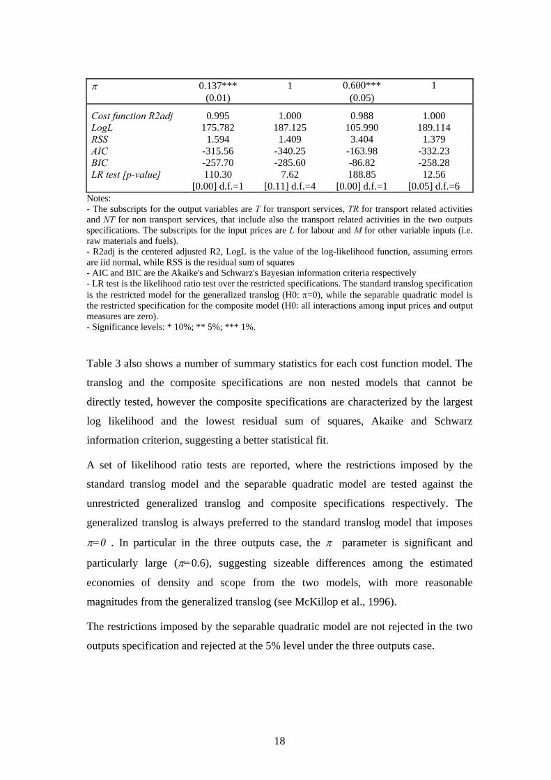
π 0.137*** 1 0.600*** 1 (0.01) (0.05)
Cost function R2adj 0.995 1.000 0.988 1.000 LogL 175.782 187.125 105.990 189.114 RSS 1.594 1.409 3.404 1.379 AIC -315.56 -340.25 -163.98 -332.23 BIC -257.70 -285.60 -86.82 -258.28 LR test [p-value] 110.30
[0.00] d.f.=1 7.62
[0.11] d.f.=4 188.85
[0.00] d.f.=1 12.56
[0.05] d.f.=6 Notes: - The subscripts for the output variables are T for transport services, TR for transport related activities and NT for non transport services, that include also the transport related activities in the two outputs specifications. The subscripts for the input prices are L for labour and M for other variable inputs (i.e. raw materials and fuels). - R2adj is the centered adjusted R2, LogL is the value of the log-likelihood function, assuming errors are iid normal, while RSS is the residual sum of squares - AIC and BIC are the Akaike's and Schwarz's Bayesian information criteria respectively - LR test is the likelihood ratio test over the restricted specifications. The standard translog specification is the restricted model for the generalized translog (H0: π=0), while the separable quadratic model is the restricted specification for the composite model (H0: all interactions among input prices and output measures are zero). - Significance levels: * 10%; ** 5%; *** 1%.
Table 3 also shows a number of summary statistics for each cost function model. The
translog and the composite specifications are non nested models that cannot be
directly tested, however the composite specifications are characterized by the largest
log likelihood and the lowest residual sum of squares, Akaike and Schwarz
information criterion, suggesting a better statistical fit.
A set of likelihood ratio tests are reported, where the restrictions imposed by the
standard translog model and the separable quadratic model are tested against the
unrestricted generalized translog and composite specifications respectively. The
generalized translog is always preferred to the standard translog model that imposes
π=0 . In particular in the three outputs case, the π parameter is significant and
particularly large (π=0.6), suggesting sizeable differences among the estimated
economies of density and scope from the two models, with more reasonable
magnitudes from the generalized translog (see McKillop et al., 1996).
The restrictions imposed by the separable quadratic model are not rejected in the two
outputs specification and rejected at the 5% level under the three outputs case.

19
6. Economies of scope and size
Scope and density economies are computed using all the estimated specifications.
Table 4 presents the results for the generalized translog and the composite
specifications, while table 3A in the appendix reports the results for the four
specifications (standard translog, generalized translog, separable quadratic and
composite).
As expected results significantly change with different outputs’ definitions and cost
function specifications.
Scope economies for the median firm range between 16% and 30% depending on the
output definition and the chosen cost function. For a two outputs technology,
economies of scope are not significantly different from zero under the generalized
translog model, while they are precisely estimated and amount to 16% when the
composite specification is used.
Results from the three outputs models are also conflicting: both estimates are
significantly different from zero, but the magnitude almost double when moving from
the generalized translog to the composite model (16% vs. 30%).
Global scope economies for the median public firm are significantly different from
zero for both the composite models and the generalized translog with three outputs
and they range between -13% and 17%. Economies of scope for privately owned firms
range between 16% and 29%. In general lower global scope economies for public
firms are always found and in one case diseconomies arise (i.e. the joint production of
three outputs leads to higher costs than a disjoint production).
Table 4 also reports global and product specific density economies. They are always
significant (except for the product specific density returns from the two outputs
generalized translog) and global density economies point towards the presence of
moderate economies of size: proportionally increasing the operating size for all
outputs, lower average costs can be achieved.
Results from the product specific density returns are mixed: from the composite model
absence of economies or small diseconomies of size are obtained, while the
generalized translog reports large density economies for the non transport services
(1.58) that are operated at a too low scale.
20
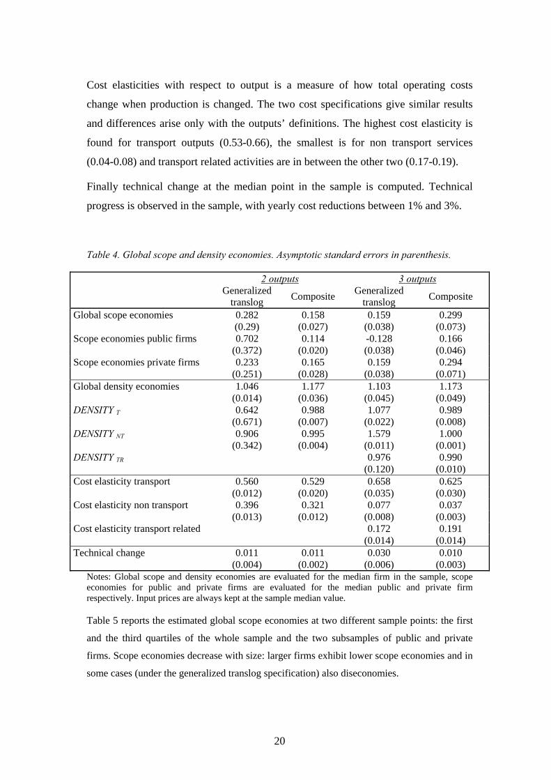
Cost elasticities with respect to output is a measure of how total operating costs
change when production is changed. The two cost specifications give similar results
and differences arise only with the outputs’ definitions. The highest cost elasticity is
found for transport outputs (0.53-0.66), the smallest is for non transport services
(0.04-0.08) and transport related activities are in between the other two (0.17-0.19).
Finally technical change at the median point in the sample is computed. Technical
progress is observed in the sample, with yearly cost reductions between 1% and 3%.
Table 4. Global scope and density economies. Asymptotic standard errors in parenthesis.
2 outputs 3 outputs
Generalized translog Composite Generalized
translog Composite
Global scope economies 0.282 0.158 0.159 0.299 (0.29) (0.027) (0.038) (0.073) Scope economies public firms 0.702 0.114 -0.128 0.166 (0.372) (0.020) (0.038) (0.046) Scope economies private firms 0.233 0.165 0.159 0.294 (0.251) (0.028) (0.038) (0.071) Global density economies 1.046 1.177 1.103 1.173 (0.014) (0.036) (0.045) (0.049) DENSITY T 0.642 0.988 1.077 0.989 (0.671) (0.007) (0.022) (0.008) DENSITY NT 0.906 0.995 1.579 1.000 (0.342) (0.004) (0.011) (0.001) DENSITY TR 0.976 0.990 (0.120) (0.010) Cost elasticity transport 0.560 0.529 0.658 0.625 (0.012) (0.020) (0.035) (0.030) Cost elasticity non transport 0.396 0.321 0.077 0.037 (0.013) (0.012) (0.008) (0.003) Cost elasticity transport related 0.172 0.191 (0.014) (0.014) Technical change 0.011 0.011 0.030 0.010 (0.004) (0.002) (0.006) (0.003)
Notes: Global scope and density economies are evaluated for the median firm in the sample, scope economies for public and private firms are evaluated for the median public and private firm respectively. Input prices are always kept at the sample median value.
Table 5 reports the estimated global scope economies at two different sample points: the first
and the third quartiles of the whole sample and the two subsamples of public and private
firms. Scope economies decrease with size: larger firms exhibit lower scope economies and in
some cases (under the generalized translog specification) also diseconomies.

21
Table 5. Estimated global scope economies at different sample points: generalized translog
and composite specifications, 3 outputs. Asymptotic standard errors in parenthesis.
Generalized translog (3 outputs)
Composite (3 outputs)
Whole sample 1st quartile 0.624 (0.043) 0.574 (0.124) 3rd quartile -0.103 (0.059) 0.148 (0.038) Public firms 1st quartile 0.780 (0.061) 0.805 (0.148) 3rd quartile -0.334 (0.054) 0.152 (0.047) Private firms 1st quartile 0.574 (0.041) 0.534 (0.118) 3rd quartile -0.085 (0.041) 0.204 (0.050)
We suspect that the differing global scope economies for the two groups of firms (public and
private) are the result of two effects: on one side the size effect; on the other side the effect of
different diversification strategies. In general public firms are larger than private firms and
they exhibit lower global scope economies as table 5 makes clear. Moreover public firms
mainly diversify in regulated industries (non transport services), while private firms in
competitive markets (transport related activities) and we are interested in the sign and
dimension of the scope economies deriving from the strategic choice of diversification. In
order to disentangle these effects, we follow Fraquelli et al. (2005), computing global scope
economies for different combination of the three outputs.
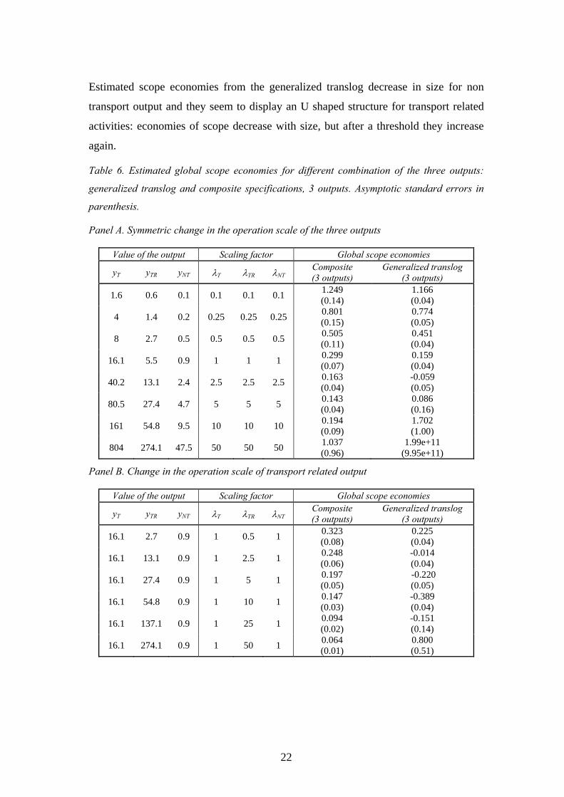
Table 6 presents the estimated scope economies when the scale of operation of the
median firm in the whole sample is increased or reduced proportionally. λi is the
scaling factor for output i: when λi = 1 the output is at its median value, when λ>(<)1
the output value is proportionally increased (decreased) with respect to its median
point.
Sizeable scope economies are found for any combination of the scaling factors (see
panel A of table 6). Scope economies always decrease with the operating dimension
and they often are statistically significant, in particular when the size is very large, the
estimates are not precise and display large standard errors
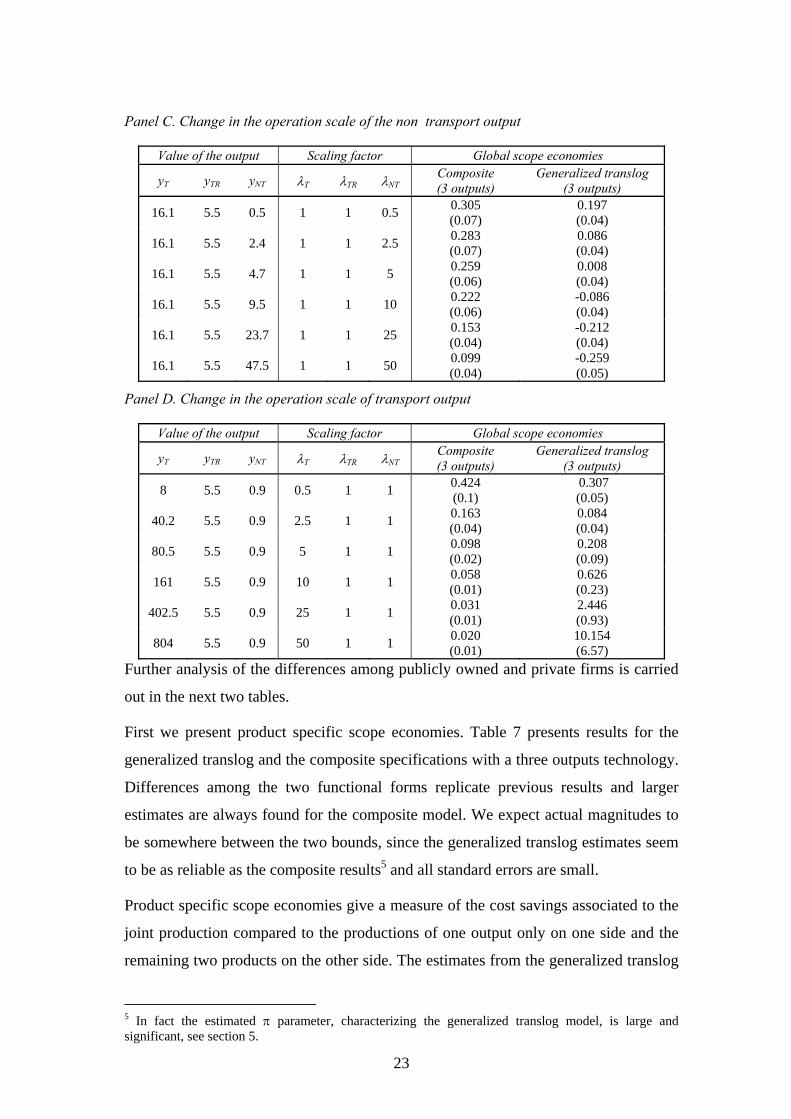
Panel B and C present scope economies when the operation size of transport related
and non transport services is increased. Scope economies decrease with dimension but
they always are positive and significant under the composite specification. Scope
economies decrease more steadily when transport related services are considered,
while scope economies are still sizeable (about 10%) when the output is 50 times the
sample median level and the composite specification is considered.
22
Estimated scope economies from the generalized translog decrease in size for non
transport output and they seem to display an U shaped structure for transport related
activities: economies of scope decrease with size, but after a threshold they increase
again.
Table 6. Estimated global scope economies for different combination of the three outputs:
generalized translog and composite specifications, 3 outputs. Asymptotic standard errors in
parenthesis.
Panel A. Symmetric change in the operation scale of the three outputs
Value of the output Scaling factor Global scope economies
yT yTR yNT λT λTR λNT Composite (3 outputs)
Generalized translog (3 outputs)
1.6 0.6 0.1 0.1 0.1 0.1 1.249 (0.14)
1.166 (0.04)
4 1.4 0.2 0.25 0.25 0.25 0.801 (0.15)
0.774 (0.05)
8 2.7 0.5 0.5 0.5 0.5 0.505 (0.11)
0.451 (0.04)
16.1 5.5 0.9 1 1 1 0.299 (0.07)
0.159 (0.04)
40.2 13.1 2.4 2.5 2.5 2.5 0.163 (0.04)
-0.059 (0.05)
80.5 27.4 4.7 5 5 5 0.143 (0.04)
0.086 (0.16)
161 54.8 9.5 10 10 10 0.194 (0.09)
1.702 (1.00)
804 274.1 47.5 50 50 50 1.037 (0.96)
1.99e+11 (9.95e+11)
Panel B. Change in the operation scale of transport related output
Value of the output Scaling factor Global scope economies
yT yTR yNT λT λTR λNT Composite (3 outputs)
Generalized translog (3 outputs)
16.1 2.7 0.9 1 0.5 1 0.323 (0.08)
0.225 (0.04)
16.1 13.1 0.9 1 2.5 1 0.248 (0.06)
-0.014 (0.04)
16.1 27.4 0.9 1 5 1 0.197 (0.05)
-0.220 (0.05)
16.1 54.8 0.9 1 10 1 0.147 (0.03)
-0.389 (0.04)
16.1 137.1 0.9 1 25 1 0.094 (0.02)
-0.151 (0.14)
16.1 274.1 0.9 1 50 1 0.064 (0.01)
0.800 (0.51)
23
Panel C. Change in the operation scale of the non transport output
Value of the output Scaling factor Global scope economies
yT yTR yNT λT λTR λNT Composite (3 outputs)
Generalized translog (3 outputs)
16.1 5.5 0.5 1 1 0.5 0.305 (0.07)
0.197 (0.04)
16.1 5.5 2.4 1 1 2.5 0.283 (0.07)
0.086 (0.04)
16.1 5.5 4.7 1 1 5 0.259 (0.06)
0.008 (0.04)
16.1 5.5 9.5 1 1 10 0.222 (0.06)
-0.086 (0.04)
16.1 5.5 23.7 1 1 25 0.153 (0.04)
-0.212 (0.04)
16.1 5.5 47.5 1 1 50 0.099 (0.04)
-0.259 (0.05)
Panel D. Change in the operation scale of transport output
Value of the output Scaling factor Global scope economies
yT yTR yNT λT λTR λNT Composite (3 outputs)
Generalized translog (3 outputs)
8 5.5 0.9 0.5 1 1 0.424 (0.1)
0.307 (0.05)
40.2 5.5 0.9 2.5 1 1 0.163 (0.04)
0.084 (0.04)
80.5 5.5 0.9 5 1 1 0.098 (0.02)
0.208 (0.09)
161 5.5 0.9 10 1 1 0.058 (0.01)
0.626 (0.23)
402.5 5.5 0.9 25 1 1 0.031 (0.01)
2.446 (0.93)
804 5.5 0.9 50 1 1 0.020 (0.01)
10.154 (6.57)
Further analysis of the differences among publicly owned and private firms is carried
out in the next two tables.
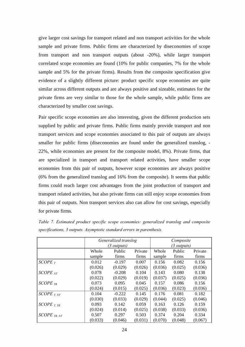
First we present product specific scope economies. Table 7 presents results for the
generalized translog and the composite specifications with a three outputs technology.
Differences among the two functional forms replicate previous results and larger
estimates are always found for the composite model. We expect actual magnitudes to
be somewhere between the two bounds, since the generalized translog estimates seem
to be as reliable as the composite results5 and all standard errors are small.
Product specific scope economies give a measure of the cost savings associated to the
joint production compared to the productions of one output only on one side and the
remaining two products on the other side. The estimates from the generalized translog
5 In fact the estimated π parameter, characterizing the generalized translog model, is large and significant, see section 5.
24
give larger cost savings for transport related and non transport activities for the whole
sample and private firms. Public firms are characterized by diseconomies of scope
from transport and non transport outputs (about -20%), while larger transport
correlated scope economies are found (10% for public companies, 7% for the whole
sample and 5% for the private firms). Results from the composite specification give
evidence of a slightly different picture: product specific scope economies are quite
similar across different outputs and are always positive and sizeable, estimates for the
private firms are very similar to those for the whole sample, while public firms are
characterized by smaller cost savings.
Pair specific scope economies are also interesting, given the different production sets
supplied by public and private firms. Public firms mainly provide transport and non
transport services and scope economies associated to this pair of outputs are always
smaller for public firms (diseconomies are found under the generalized translog, -
22%, while economies are present for the composite model, 8%). Private firms, that
are specialized in transport and transport related activities, have smaller scope
economies from this pair of outputs, however scope economies are always positive
(6% from the generalized translog and 16% from the composite). It seems that public
firms could reach larger cost advantages from the joint production of transport and
transport related activities, but also private firms can still enjoy scope economies from
this pair of outputs. Non transport services also can allow for cost savings, especially
for private firms.
Table 7. Estimated product specific scope economies: generalized translog and composite
specifications, 3 outputs. Asymptotic standard errors in parenthesis.
Generalized translog (3 outputs)
Composite (3 outputs)
Whole sample
Public firms
Private firms
Whole sample
Public firms
Private firms
SCOPE T 0.012 -0.197 0.007 0.156 0.082 0.156 (0.026) (0.029) (0.026) (0.036) (0.025) (0.036) SCOPE NT 0.078 -0.208 0.104 0.143 0.080 0.138 (0.022) (0.029) (0.019) (0.037) (0.025) (0.036) SCOPE TR 0.073 0.095 0.045 0.157 0.086 0.156 (0.024) (0.015) (0.025) (0.036) (0.023) (0.036) SCOPE T, NT 0.104 -0.222 0.145 0.176 0.081 0.182 (0.030) (0.033) (0.029) (0.044) (0.025) (0.046) SCOPE T, TR 0.093 0.142 0.059 0.163 0.126 0.159 (0.024) (0.014) (0.025) (0.038) (0.033) (0.036) SCOPE TR, NT 0.507 0.297 0.503 0.374 0.204 0.334 (0.033) (0.046) (0.031) (0.070) (0.048) (0.067)

25
Notes: All magnitudes are evaluated for the median firm in the sample, scope economies for public and private firms are evaluated for the median public and private firm respectively. Input prices are always kept at the sample median value.
Finally it is possible to split global scope economies into the fixed costs savings and
the variable inputs cost complementarities for the composite model. Table 8 shows the
estimates from the two outputs and three outputs technology, since from expression
(3) it is evident that the contribution to economies of scope from fixed costs savings
increases with the number of outputs and it could be interesting to compare the
different magnitudes. The largest cost savings are associated to fixed costs and they
range between 10% (public firms) and 16% (private companies) in the two outputs
cost model and 17% (public firms) and 28% (private companies) in the three outputs
model. Cost complementarities are small and in some cases not significantly different
from zero (for private firms in the two outputs case and for public firms in the three
outputs model). Fixed cost savings from the joint production of different outputs may
be associated to the possibility to share fixed assets, like the rolling stock, the
hardware and software organization, buildings, offices and parking areas. Cost savings
from the variable inputs that can be shared by different product lines, are modest,
probably because the most important variable input is labour (accounting for about
45% of total costs) that is not completely interchangeable between transport and other
services.
As discussed in section 3, however it is worth to stress that the estimated fixed costs
savings represent an upper bound estimate of the true savings.
Table 8. Fixed costs and cost complementarities effects: composite specifications, 2 and 3
outputs. Asymptotic standard errors in parenthesis.
Composite 2 outputs
Composite 3 outputs
Whole sample
Public firms
Private firms
Whole sample
Public firms
Private firms
Fixed costs savings 0.151 0.102 0.158 0.286 0.169 0.277 (0.027) (0.019) (0.028) (0.074) (0.046) (0.072) Cost complementarities 0.007 0.012 0.007 0.013 -0.003 0.017 (0.006) (0.009) (0.005) (0.007) (0.015) (0.008) Notes: All magnitudes are evaluated for the median firm in the sample, scope economies for public and private firms are evaluated for the median public and private firm respectively. Input prices are always kept at the sample median value.
26
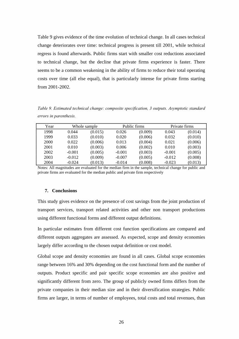
Table 9 gives evidence of the time evolution of technical change. In all cases technical
change deteriorates over time: technical progress is present till 2001, while technical
regress is found afterwards. Public firms start with smaller cost reductions associated
to technical change, but the decline that private firms experience is faster. There
seems to be a common weakening in the ability of firms to reduce their total operating
costs over time (all else equal), that is particularly intense for private firms starting
from 2001-2002.
Table 9. Estimated technical change: composite specification, 3 outputs. Asymptotic standard
errors in parenthesis.
Year Whole sample Public firms Private firms 1998 0.044 (0.015) 0.026 (0.009) 0.043 (0.014) 1999 0.033 (0.010) 0.020 (0.006) 0.032 (0.010) 2000 0.022 (0.006) 0.013 (0.004) 0.021 (0.006) 2001 0.010 (0.003) 0.006 (0.002) 0.010 (0.003) 2002 -0.001 (0.005) -0.001 (0.003) -0.001 (0.005) 2003 -0.012 (0.009) -0.007 (0.005) -0.012 (0.008) 2004 -0.024 (0.013) -0.014 (0.008) -0.023 (0.013)
Notes: All magnitudes are evaluated for the median firm in the sample, technical change for public and private firms are evaluated for the median public and private firm respectively
7. Conclusions
This study gives evidence on the presence of cost savings from the joint production of
transport services, transport related activities and other non transport productions
using different functional forms and different output definitions.
In particular estimates from different cost function specifications are compared and
different outputs aggregates are assessed. As expected, scope and density economies
largely differ according to the chosen output definition or cost model.
Global scope and density economies are found in all cases. Global scope economies
range between 16% and 30% depending on the cost functional form and the number of
outputs. Product specific and pair specific scope economies are also positive and
significantly different from zero. The group of publicly owned firms differs from the
private companies in their median size and in their diversification strategies. Public
firms are larger, in terms of number of employees, total costs and total revenues, than

27
private firms and they mainly supply subsidized local public transportation services
and non transport services.
Private firms mainly supply subsidized local public transportation services and non
subsidized transport related activities. Global scope economies are larger for private
firms (between 16% and 30%), while diseconomies of scope are found for public
firms in one specification (estimated global scope economies range between -13% and
17%). It is possible to split estimated global scope economies (from the composite
specifications) into fixed costs savings and cost complementarities effects. Larger
costs savings result from fixed costs, especially for private firms.
The general picture seems to be characterized by local public transport firms that
enjoy global scope economies, that are particularly high for private firms. Public firms
are characterized by lower scope economies, and sometimes diseconomies, probably
because of their chosen production structure where a large and heterogeneous set of
non transport services is supplied together with transport.
28
8. References
Adams R.M., Bauer P.W. and Sickle R.C., 2004, ‘Scale economies, scope economies
and technical change in Federal Reserve payment processing’, Journal of
Money Credit and Banking, 36, 943-958
Asai S., 2006, ‘Scale economies and scope economies in the Japanese broadcasting
market’, Information Economics and Policy, 18, 321-331
Barnett W.A. and Lee Y.W., 1985, ‘The global properties of the Miniflex Laurent,
Generalised Leontief and Translog Flexible functional forms’, Econometrica,
53, 1421-1437
Baumol W.J., Panzar J.C. and Willig R.D., 1982, Contestable markets and the theory
of industry structure, New York, Harcourt, Brace, Jovanovich, Inc.
Bloch H., Madden G., Savage S. J., 2001, ‘Economies of scale and scope in Australian
telecommunications’, Review of Industrial Organization, 18, 219-227
Box G. and Cox D., 1964, ‘An analysis of transformations’, Journal of the Royal
Statistical Society, Series B, 26, 211-246
Cameron A.C. and Trivedi P.K., 2005, Microeconometrics. Methods and
Applications, New York: Cambridge University Press
Carrol R. and Rupert D., 1984, ‘Power transformations when fitting theoretical
models to data’, Journal of the American Statistics Association, 79, 321-328
Carrol R. and Rupert D., 1988, Transformation and Weighting in Regressions, New
York: Chapman & Hill
Caves D.W., Christensen L.R. and Tretheway M.W., 1980, Flexible cost functions for
multiproduct firms, Review of Economics and Statistics, 62, 477-481
Caves D.W., Christensen L.R. and Tretheway M.W., 1984, Economies of density
versus economies of scale: why trunk and local airline costs differ, Rand
Journal of Economics, 15, 471-489
Christensen L. and Jorgenson D.W., 1969, ‘The measurement of U.S. real capital
input, 1929–67’, Review of Income and Wealth, 15, 293–320
Christensen L.R., Jorgenson D.W. and Lau L.J., 1971, ‘Conjugate duality and the
transcendental logarithmic production function’, Econometrica, 39, 255-256

29
Colburn C.B. and Talley W.K., 1992, ‘A firm specific analysis of economies of size in
the U.S. urban multiservice transit industry’, Transportation Research Part B,
3, 195-206
Cowie J. and Asenova D., 1999, ‘Organisation form, scale effects and efficiency in the
British bus industry’, Transportation, 26, 231- 248
De Borger B., Kerstens K. and Costa A., 2002, ‘Public transit performance: what does
one learn from frontier studies?’, Transport Reviews, 22(1), 1-38
Diewert W.E., 1974, ‘Applications of duality theory’, in ‘Frontiers in Quantitative
Economics’, Vol 2 (Eds.) M. D. Intriligator and D. A. Kendrick, North
Holland, Amsterdam, pp. 106 – 171
Diewert W.E. and Wales T.J., 1987, ‘Flexible functional forms and global curvature
conditions’, Econometrica, 55(1), 43-68
Di Giacomo M. and Ottoz E., 2007, ‘Local public transportation firms: the relevance
of scale and scope economies in the provision of urban and intercity bus
transit’, mimeo
Farsi M., Fetz A. and Filippini M., 2007, ‘Economies of scale and scope in local
public transportation’, Journal of Transport Economics and Policy,
forthcoming
Fraquelli G., Piacenza M. and Abrate G, 2004a, ‘Regulating Public Transit Systems:
How Do Urban-Intercity Diversification and Speed-up Measures Affect Firms’
Cost Performance?’, Annals of Public and Cooperative Economics, 75(2), 193-
225
Fraquelli G., Piacenza M. and Vannoni D., 2004b, ‘Scope and scale economies in
multi-utilities: evidence from gas, water and electricity combinations’, Applied
Economics, 36, 2045-2057
Fraquelli G., Piacenza M. and Vannoni D., 2005, ‘Cost Savings from Generation and
Distribution with an Application to Italian Electric Utilities’, Journal of
Regulatory Economics, 28(3), 289-308
Lancaster T., 2000, ‘The incidental parameter problem since 1948’, Journal of
Econometrics, 95, 391-413.

30
McKenzie D.J. and Small J.P., 1997, ‘Econometric cost structure estimates for cellular
telephony in the United States, Journal of Regulatory Economics, 12, 147-157
McKillop D.G., Glass J.C. and Morikawa Y., 1996, ‘The composite cost function and
efficiency in giant Japanese banks’, Journal of Banking and Finance, 20,
1651-1671
Ottoz E., Fornengo G. and Di Giacomo M., 2007, ‘The impact of ownership on the
cost of bus service provision: an example from Italy’, Applied Economics,
forthcoming
Piacenza M. and Vannoni D., 2004, ‘Choosing Among Alternative Cost Function
Specifications: An Application to Italian Multi-Utilities’, Economics Letters,
82(3), 410-417
Pulley L.B. and Braunstein Y.M., 1992, ‘A composite cost function for multiproduct
firms with an application to economies of scope in banking’, Review of
Economics and Statistics, 74, 221-230
Pulley L.B. and Humphrey D.B., 1993, ‘Scope economies: Fixed costs,
complementarity and functional form’, Journal of Business, 66(3), 437-462
Roller L.-H., 1990, ‘Proper quadratic cost functions with an application to the Bell
System’, Review of Economics and Statistics, 72, 202-210.
Silk A. and Berndt E., 2004, ‘Holding companies cost economies in the global
advertising and marketing services business ’, Review of Marketing Science, 2,
Viton P., 1992, ‘Consolidations of scale and scope in urban transit’, Regional Science
and Urban Economics, 22, 25-49
Viton P., 1993, ‘How big should transit be? Evidence from San Francisco bay area’,
Transportation, 20, 35-57

31
Appendix
Table 1A. Estimation results: 2 outputs (transport, yT , and other non transport services, yNT),
3 inputs. Dependent variable: natural logarithm of total operating costs normalized by the
price of capital. Unbalanced panel: 40 firms, 184 observations. Cluster robust standard
errors in parenthesis.
Dependent variables
Standard Translog
Generalized Translog
Separable quadratic Composite
yT 0.558 0.560 1714.680 1691.533 (0.01) (0.01) (53.58) (58.20) yNT 0.451 0.396 1052.752 1050.135 (0.02) (0.01) (29.50) (28.89) yT2 0.230 0.136 31.472 41.682 (0.02) (0.02) (25.37) (24.80) yNT2 0.059 0.092 12.575* 10.362 (0.01) (0.01) (7.09) (8.58) yNT*yT -0.245 -0.287 -53.536* -46.327 (0.01) (0.01) (30.35) (36.08) yT*lnpL -0.154** -0.148 -852.265 (0.07) (0.03) (155.77) yNT*lnpL 0.255** 0.124** -156.916 (0.07) (0.04) (121.34) yT*lnpM 0.080 0.101** 1187.209 (0.07) (0.04) (325.18) yNT*lnpM -0.215** -0.122** 427.031** (0.07) (0.05) (187.02) Trend -0.090** -0.112 -210.817** -189.490** (0.03) (0.02) (63.27) (56.99) Trend2 0.023 0.025 43.046** 38.345** (0.01) (0.01) (15.53) (13.87) lnpL 0.288 0.226 0.271 0.585 (0.06) (0.05) (0.06) (0.05) lnpL2 -0.233 -0.211 -0.166 0.233 (0.04) (0.04) (0.05) (0.26) lnpM 0.175 0.181 0.171 0.182 (0.07) (0.07) (0.06) (0.17) lnpM2 0.086 0.029 -0.243 0.450 (0.30) (0.26) (0.21) (0.38) lnpL*lnpM 0.149 0.117 0.203* -0.311 (0.14) (0.13) (0.10) (0.24) Constant 8.143 8.176 532.534 488.800 (0.05) (0.04) (102.84) (101.17) π 0 0.137 1 1 (0.01)
Cost funct. R2adj 0.990 0.995 1.000 1.000 LogL 120.630 175.782 183.315 187.125 RSS 2.903 1.594 1.469 1.409 AIC -207.26 -315.56 -340.63 -340.25 BIC -152.61 -257.70 -298.84 -285.60

32
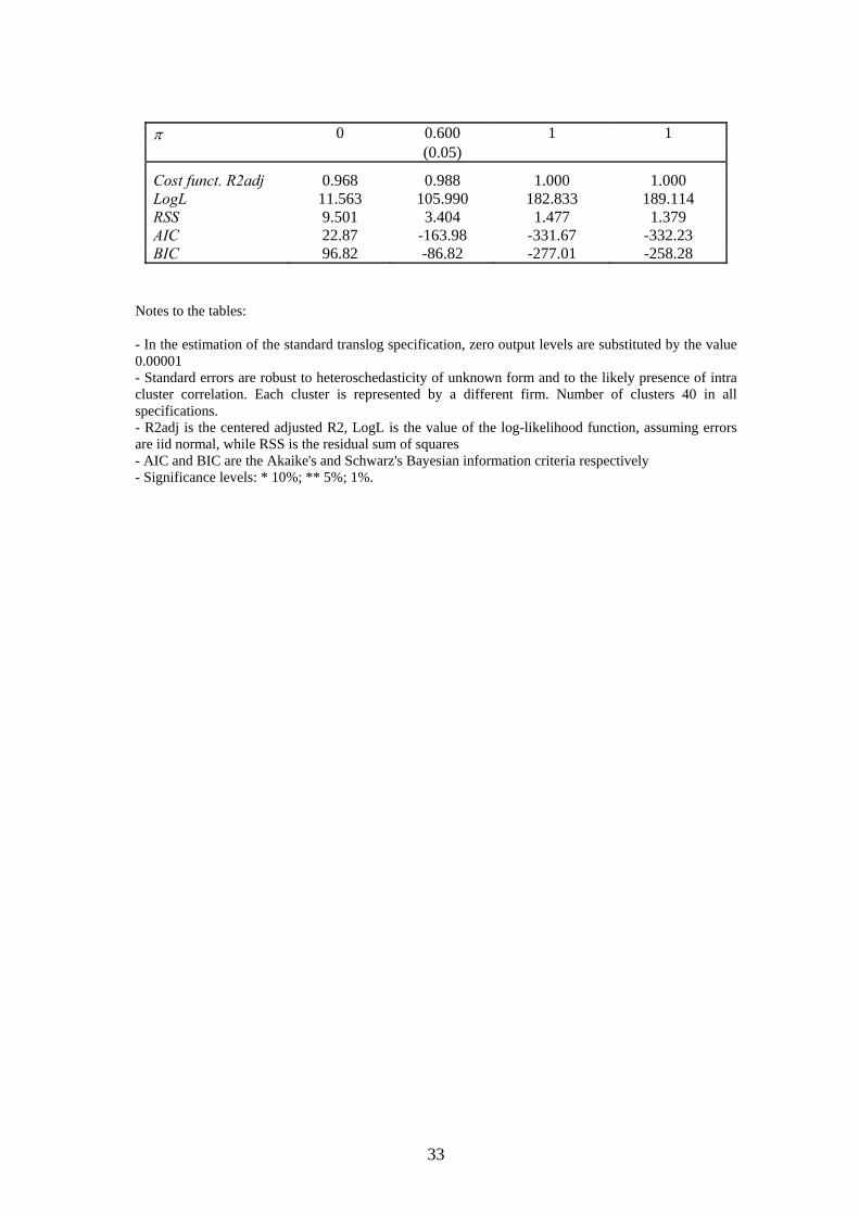
Table 2A. Estimation results: 3 outputs (transport, yT , transport related activities, yTR , and
other non transport services, yNT), 3 inputs. Dependent variable: natural logarithm of total
operating costs normalized by the price of capital. Unbalanced panel: 40 firms, 184
observations. Cluster robust standard errors in parenthesis.
Dependent variables
Standard Translog
Generalized Translog
Separable quadratic Composite
yT 0.620 0.658 1711.710 1700.896 (0.04) (0.04) (56.50) (63.97) yNT 0.069 0.077 99.461 99.285 (0.01) (0.01) (6.34) (6.81) yTR 0.128 0.172 539.380 545.735 (0.03) (0.01) (27.39) (29.79) yT2 0.201 -0.098 32.724 38.188 (0.04) (0.02) (26.13) (25.52) yNT2 0.008 -0.001** 0.060 0.037 (0.00) (0.00) (0.09) (0.12) yTR2 0.008* 0.074 10.844 10.704 (0.00) (0.02) (8.86) (9.56) yT *yNT 0.030** -0.046 2.309 1.972 (0.01) (0.01) (5.55) (5.81) yT *yTR 0.056 -0.142 -68.875* -74.822** (0.01) (0.02) (35.27) (33.50) yTR *yNT -0.062 -0.011 -0.330 0.317 (0.01) (0.00) (2.74) (3.11) yT *lnpL -0.243** -0.131* -937.415 (0.11) (0.07) (167.38) yNT *lnpL 0.010 -0.015 -7.039 (0.01) (0.01) (11.10) yTR *lnpL 0.015 -0.099 -237.887** (0.03) (0.07) (79.23) yT *lnpM 0.118 0.112** 1515.650 (0.14) (0.05) (199.39) yNT *lnpM -0.030 0.014 45.327** (0.02) (0.01) (12.99) yTR *lnpM -0.035 0.090 468.431 (0.03) (0.07) (91.15) Trend -0.096 -0.145 -206.272** -152.146** (0.06) (0.03) (62.58) (58.10) Trend2 0.021 0.029** 41.488** 31.030** (0.01) (0.01) (15.41) (13.47) lnpL 0.438** 0.395** 0.269 0.685 (0.21) (0.13) (0.05) (0.06) lnpL2 -0.433** -0.423 -0.176 0.810** (0.15) (0.10) (0.04) (0.33) lnpM 0.151 0.154 0.172 0.170 (0.18) (0.13) (0.06) (0.11) lnpM2 -0.356 -0.051 -0.192 1.861** (0.65) (0.42) (0.22) (0.68) lnpL*lnpM 0.512 0.258 0.185* -1.235** (0.33) (0.23) (0.11) (0.46) Constant 8.089 8.064 540.743 389.278** (0.10) (0.06) (103.88) (115.78)
33
π 0 0.600 1 1 (0.05)
Cost funct. R2adj 0.968 0.988 1.000 1.000 LogL 11.563 105.990 182.833 189.114 RSS 9.501 3.404 1.477 1.379 AIC 22.87 -163.98 -331.67 -332.23 BIC 96.82 -86.82 -277.01 -258.28
Notes to the tables:
- In the estimation of the standard translog specification, zero output levels are substituted by the value 0.00001 - Standard errors are robust to heteroschedasticity of unknown form and to the likely presence of intra cluster correlation. Each cluster is represented by a different firm. Number of clusters 40 in all specifications. - R2adj is the centered adjusted R2, LogL is the value of the log-likelihood function, assuming errors are iid normal, while RSS is the residual sum of squares - AIC and BIC are the Akaike's and Schwarz's Bayesian information criteria respectively - Significance levels: * 10%; ** 5%; 1%.

34
Table 3A. Global scope and density economies. Asymptotic standard errors in parenthesis.
Panel (a). 2 outputs, 3 inputs
Std. translog Generalized translog Separable quadratic Composite Global scope economies 1526067.8 0.282 0.170 0.158 (9.58e+07) (0.29) (0.027) (0.027) Scope economies public firms 2584624.7 0.702 0.124 0.114 (2.56e+8) (0.372) (0.021) (0.020) Scope economies private firms 1266425.6 0.233 0.176 0.165 (7.48e+07) (0.251) (0.028) (0.028) Global density economies 0.992 1.046 1.195 1.177 (0.025) (0.014) (0.038) (0.036) DENSITY T -2.74E+06 0.642 0.991 0.988 (5.01E+06) (0.671) (0.007) (0.007) DENSITY NT 1.006 0.906 0.994 0.995 (0.444) (0.342) (0.004) (0.004) Cost elasticity transport 0.558 0.560 0.522 0.529 (0.013) (0.012) (0.019) (0.020) Cost elasticity non transport 0.451 0.396 0.315 0.321 (0.019) (0.013) (0.014) (0.012)
Panel (b). 3 outputs, 3 inputs
Std. translog Generalized translog Separable quadratic Composite Global scope economies 3927109 0.159 0.387 0.299 (1.42E+07) (0.038) (0.061) (0.073) Scope economies public firms 5203062 -0.128 0.223 0.166 (1.89E+07) (0.038) (0.041) (0.046) Scope economies private firms 3389150 0.159 0.380 0.294 (1.23E+07) (0.038) (0.060) (0.071) Global density economies 1.224 1.103 1.237 1.173 (0.065) (0.045) (0.047) (0.049) DENSITY T -6.51E+04 1.077 0.990 0.989 (2.93E+05) (0.022) (0.008) (0.008) DENSITY NT 2.403 1.579 1.000 1.000 (0.951) (0.011) (0.000) (0.001) DENSITY TC 4.848 0.976 0.989 0.990 (1.290) (0.120) (0.009) (0.010) Cost elasticity transport 0.620 0.658 0.594 0.625 (0.040) (0.035) (0.024) (0.030) Cost elasticity non transport 0.069 0.077 0.035 0.037 (0.013) (0.008) (0.003) (0.003) Cost elasticity transport related 0.128 0.172 0.179 0.191 (0.031) (0.014) (0.014) (0.014)
Notes: Global scope and density economies are evaluated for the median firm in the sample, scope economies for public and private firms are evaluated for the median public and private firm respectively. In the computation of scope economies for the standard translog model, zero output levels are substituted with 0.000001.