Diverse Branch Block: Building a Convolution as an Inception-like Unit

Xiaohan Ding 1* Xiangyu Zhang 2 Jungong Han 3 Guiguang Ding 1†

1 Beijing National Research Center for Information Science and Technology (BNRist);School of Software, Tsinghua University, Beijing, China

2 MEGVII Technology3 Computer Science Department, Aberystwyth University, SY23 3FL, UK

dxh17@mails.tsinghua.edu.cn zhangxiangyu@megvii.com

jungonghan77@gmail.com dinggg@tsinghua.edu.cn

Abstract

We propose a universal building block of ConvolutionalNeural Network (ConvNet) to improve the performancewithout any inference-time costs. The block is named Di-verse Branch Block (DBB), which enhances the representa-tional capacity of a single convolution by combining diversebranches of different scales and complexities to enrich thefeature space, including sequences of convolutions, multi-scale convolutions, and average pooling. After training, aDBB can be equivalently converted into a single conv layerfor deployment. Unlike the advancements of novel Con-vNet architectures, DBB complicates the training-time mi-crostructure while maintaining the macro architecture, sothat it can be used as a drop-in replacement for regularconv layers of any architecture. In this way, the model canbe trained to reach a higher level of performance and thentransformed into the original inference-time structure forinference. DBB improves ConvNets on image classification(up to 1.9% higher top-1 accuracy on ImageNet), objectdetection and semantic segmentation. The PyTorch codeand models are released at https://github.com/DingXiaoH/DiverseBranchBlock.

1. IntroductionImproving the performance of Convolutional Neural

Network (ConvNet) has always been a heated researchtopic. On one hand, the advancements in architecture de-sign, e.g., the Inception models [27, 28, 26, 15], have re-

*This work is supported by The National Key Research and Develop-ment Program of China (No. 2017YFA0700800), the National NaturalScience Foundation of China (No.61925107, No.U1936202) and BeijingAcademy of Artificial Intelligence (BAAI). Xiaohan Ding is funded by theBaidu Scholarship Program 2019 (http://scholarship.baidu.com/). This work is done during Xiaohan Ding’s internship at MEGVII.

†Corresponding author.

vealed that the multi-branch topology and combination ofvarious paths with different scales and complexities can en-rich the feature space and improve the performance. How-ever, the complicated structure usually slows down the in-ference, as a combination of small operators (e.g., concate-nation of 1 × 1 conv and pooling) is not friendly to the de-vices with strong parallel computing powers like GPU [21].

On the other hand, more parameters and connectionsusually lead to higher performance, but the size of ConvNetwe deploy cannot increase arbitrarily due to the businessrequirements and hardware constraints. Considering this,we usually judge the quality of a ConvNet by the trade-offbetween performance and inference-time costs such as thelatency, memory footprint and number of parameters. Inthe common cases, we train the models on powerful GPUworkstations and deploy them onto efficiency-sensitive de-vices, so we consider it acceptable to improve the perfor-mance with the costs of more training resources, as long asthe deployed model keeps the same size.

In this paper, we seek to insert complicated structuresinto numerous ConvNet architectures to improve the perfor-mance while keeping the original inference-time costs. Tothis end, we decouple the training-time and inference-timenetwork structure by complicating the model only duringtraining and converting it back into the original structurefor inference. Naturally, we require such extra training-timestructures to be 1) effective in improving the training-timemodel’s performance and 2) able to transform into the orig-inal inference-time structure.

For the usability and universality, we upgrade the basicConvNet component, K × K conv, into a powerful blocknamed Diverse Branch Block (DBB) (Fig. 1). As a build-ing block, DBB is complementary to the other efforts to im-prove ConvNet, e.g., architecture design [12, 24, 13, 21, 23,35], neural architecture search [2, 39, 22, 20, 19], data aug-mentation and training methods [25, 5, 33] and fulfills theabove two requirements by the following two properties:

arX

iv:2

103.

1342

5v2

[cs

.CV

] 2

9 M

ar 2

021

conv batch norm

+

Training-time DBB

1×1

input

output

K×K

1×1

AVG

1×1 K×K

input

output

K×K

nonlinearity

Inference-time DBB Training-time model Inference-time model

+

+

K×K

K×K

+

K×K

K×K

+

replace conv layers

with DBBs

AVG average pooling

Figure 1: A representative design of Diverse Branch Block (DBB). The block can be equivalently transformed into a regularconv layer for deployment, so that we can complicate the training-time microstructures of ConvNet without affecting themacro architecture (e.g., ResNet) or the inference-time structure. Note that it is only an instance we used, and one may utilizethe six transformations summarized in this paper (Sect. 3.2) to customize a DBB with more complicated structures.

• A DBB adopts a multi-branch topology with multi-scale convolutions, sequential 1 × 1 - K × K con-volutions, average pooling and branch addition. Suchoperations with various receptive fields and paths withdifferent complexities can enrich the feature space, justlike the Inception architectures.

• A DBB can be equivalently transformed into a sin-gle conv for inference. Given an architecture, we canreplace some regular conv layers with DBB to buildmore complicated miscrostructures for training, andconvert it back into the original structure so that therewill be no extra inference-time costs.

More precisely, we do not derive the parameters for in-ference before each forwarding. Instead, we convert themodel after training once for all, then we only save anduse the resultant model, and the trained model can be dis-carded. The idea of converting a DBB into a conv canbe categorized into structural re-parameterization, whichmeans parameterizing a structure with the parameters trans-formed from another structure, together with a concurrentwork [9]. Though a DBB and a regular conv layer have thesame inference-time structure, the former has higher rep-resentational capacity. Through a series of ablation experi-ments, we attribute such effectiveness to the diverse connec-tions (paths with different scales and complexities) whichresembles Inception units, and the training-time nonlinear-ity brought by batch normalization [15]. Compared to somecounterparts with duplicate paths or purely linear branches(Fig. 6), DBB shows better performance (Table. 4).

We summarize our contributions as follows.

• We propose to incorporate abundant microstructuresinto various ConvNet architectures to improve the per-

formance but keep the original macro architecture.• We propose DBB, a universal building block, and sum-

marize six transformations (Fig. 2) to convert a DBBinto a single convolution, so it is cost-free for the users.

• We present a representative Inception-like DBB in-stance and show that it improves the performance onImageNet [7] (e.g., up to 1.9% higher top-1 accuracy),COCO detection [18] and Cityscapes [4].

2. Related Work

2.1. Multi-branch Architectures

Inception [15, 26, 27, 28] architectures employed multi-branch structures to enrich the feature space, which provedthe significance of diverse connections, various receptivefields and the combination of multiple branches. DBB bor-rows the idea of using multi-branch topology, but the dif-ference lies in that 1) DBB is a building block that canbe used on numerous architectures, and 2) each branch ofDBB can be converted into a conv, so that the combinationof such branches can be merged into a single conv, whichis much faster than a real Inception unit. We will showthe superiority of diverse branches over duplicate ones (Ta-ble. 4), and the most interesting discovery is that combiningtwo branches with different representational capacity (e.g.,a 1 × 1 conv and a 3 × 3 conv) is better than two strong-capacity branches (e.g., two 3×3 convolutions), which mayin turn shed light on ConvNet architecture design.

2.2. ConvNet Components for Better Performance

There have been some novel components to improveConvNets. For examples, Squeeze-and-Excitation (SE)

block [14] and Efficient Convolutional Attention (ECA)block [29] utilizes the attention mechanism to recalibratethe features, Octave Convolution [3] reduces the spatial re-dundancy of regular convolution, Deformable Convolution[6] augments the spatial sampling locations with learnableoffsets, dilated convolution expands the receptive field [32],BlurPool [34] brings back the shift-invariance, etc. DBBis complementary to these components because it only up-grades a fundamental building block: the conv layer.

2.3. Structural Re-parameterization

This paper and a concurrent work, RepVGG [9], arethe first to use structural re-parameterization to term themethodology that parameterizes a structure with the param-eters transformed from another structure. ExpandNet [10],DO-Conv [1] and ACNet [8] can also be categorized intostructural re-parameterization in the sense that they con-vert a block into a conv. For example, ACNet uses Asym-metric Convolution Block (ACB, as shown in Fig. 6d) tostrengthen the skeleton of conv kernel (i.e., the crisscrosspart). Compared to DBB, it is also designed for improvingConvNet without extra inference-time costs. However, thedifference is that ACNet was motivated by an observationthat the parameters of the skeleton were larger in magni-tude and thus sought to make them even larger, whereas wefocus on a different perspective. We found out that aver-age pooling, 1 × 1 conv, and 1 × 1 - K × K sequentialconv are more effective, as they provide paths with differ-ent complexities, and allow the usage of more training-timenonlinearity. Besides, ACB can be viewed as a special caseof DBB, since the 1 × K and K × 1 conv layers can beaugmented to K×K via Transform VI (Fig. 2) and mergedinto the square kernel via Transform II.

2.4. Other ConvNet Re-parameterization Methods

Some works can be referred to as re-parameterization,but not structural re-parameterization. For examples, arecent NAS [20, 39] method [2] used meta-kernels to re-parameterize a kernel and supplemented the widths andheights of such meta-kernels into the search space. SoftConditional Computation (SCC) [31] or CondConv [30] canbe viewed as data-dependent kernel re-parameterization, asit generated the weights for multiple kernels of the sameshape, then derived a kernel as the weighted sum of all suchkernels to participate in the convolution. Note that SCCintroduced a significant number of parameters into the de-ployed model. These re-parameterization methods differfrom ACB and DBB in that the former “re-param” meansderiving a set of new parameters with some meta parame-ters (e.g., the meta kernels [2]) then using the new parame-ters for the other computations, while the latter means con-verting the parameters of a trained model to parameterizeanother one.

3. Diverse Branch Block3.1. The Linearity of Convolution

The parameters of a conv layer with C input channels,D output channels and kernel size K × K reside in theconv kernel, which is a 4th-order tensor F ∈ RD×C×K×K ,and an optional bias b ∈ RD. It takes a C-channel fea-ture map I ∈ RC×H×W as input and outputs a D-channelfeature map O ∈ RD×H′×W ′

, where H ′ and W ′ are deter-mined by K, padding and stride configurations. We use ~to denote the convolution operator, and formulate the bias-adding as replicating the bias b into REP(b) ∈ RD×H′×W ′

and adding it onto the results of convolution. Formally,

O = I ~ F + REP(b) . (1)

The value at (h,w) on the j-th output channel is given by

Oj,h,w =

C∑c=1

K∑u=1

K∑v=1

Fj,c,u,vX(c, h, w)u,v + bj , (2)

where X(c, h, w) ∈ RK×K is the sliding window on thec-th channel of I corresponding to the position (h,w) onO. Such a correspondence is determined by the paddingand stride. The linearity of conv can be easily derived fromEq. 2, which includes the homogeneity and additivity,

I ~ (pF ) = p(I ~ F ) ,∀p ∈ R , (3)

I ~ F (1) + I ~ F (2) = I ~ (F (1) + F (2)) . (4)

Note that the additivity holds only if the two convolutionshave the same configurations (e.g., number of channels, ker-nel size, stride, padding, etc.), so that they share the samesliding window correspondence X .

3.2. A Convolution for Diverse Branches

In this subsection, we summarize six transformations(Fig. 2) to transform a DBB with batch normalization (BN),branch addition, depth concatenation, multi-scale opera-tions, average pooling and sequences of convolutions.

Transform I: a conv for conv-BN We usually equip aconv with a BN layer, which performs channel-wise nor-malization and linear scaling. Let j be the channel index,µj and σj be the accumulated channel-wise mean and stan-dard deviation, γj and βj be the learned scaling factor andbias term, respectively, the output channel j becomes

Oj,:,: = ((I ~ F )j,:,: − µj)γjσj

+ βj . (5)

The homogeneity of conv enables to fuse BN into thepreceding conv for inference. In practice, we simply builda single conv with kernel F ′ and bias b′, assign the values

conv

batch

norm

AVGaverage

pooling

K×K

+

K×K K×K

1×1

K×K

AVG

1×1 1×K K×1

K×K

Transform I

Transform II

Transform III

Transform IV

Transform V

Transform VI

K×K K×K

concat

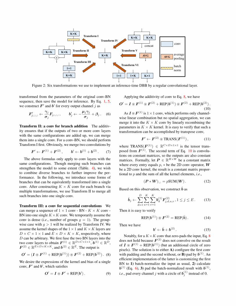
Figure 2: Six transformations we use to implement an inference-time DBB by a regular convolutional layer.

transformed from the parameters of the original conv-BNsequence, then save the model for inference. By Eq. 1, 5,we construct F ′ and b′ for every output channel j as

F ′j,:,:,: ←γjσjFj,:,:,: , b′j ← −

µjγjσj

+ βj . (6)

Transform II: a conv for branch addition The additiv-ity ensures that if the outputs of two or more conv layerswith the same configurations are added up, we can mergethem into a single conv. For a conv-BN, we should performTransform I first. Obviously, we merge two convolutions by

F ′ ← F (1) + F (2) , b′ ← b(1) + b(2) . (7)

The above formulas only apply to conv layers with thesame configurations. Though merging such branches canstrengthen the model to some extent (Table. 4), we wishto combine diverse branches to further improve the per-formance. In the following, we introduce some forms ofbranches that can be equivalently transformed into a singleconv. After constructing K × K conv for each branch viamultiple transformations, we use Transform II to merge allsuch branches into one single conv.

Transform III: a conv for sequential convolutions Wecan merge a sequence of 1 × 1 conv - BN - K ×K conv -BN into one single K×K conv. We temporarily assume theconv is dense (i.e., number of groups g = 1). The group-wise case with g > 1 will be realized by Transform IV. Weassume the kernel shapes of the 1×1 and K×K layers areD × C × 1× 1 and E ×D ×K ×K, respectively, whereD can be arbitrary. We first fuse the two BN layers into thetwo conv layers to obtain F (1) ∈ RD×C×1×1, b(1) ∈ RD,F (2) ∈ RE×D×K×K , and b(2) ∈ RE . The output is

O′ = (I ~ F (1) + REP(b(1)))~ F (2) + REP(b(2)) . (8)

We desire the expressions of the kernel and bias of a singleconv, F ′ and b′, which satisfies

O′ = I ~ F ′ + REP(b′) . (9)

Applying the additivity of conv to Eq. 8, we have

O′ = I ~ F (1) ~ F (2) + REP(b(1))~ F (2) + REP(b(2)) .(10)

As I~F (1) is 1×1 conv, which performs only channel-wise linear combination but no spatial aggregation, we canmerge it into the K ×K conv by linearly recombining theparameters in K ×K kernel. It is easy to verify that such atransformation can be accomplished by transpose conv,

F ′ ← F (2) ~ TRANS(F (1)) , (11)

where TRANS(F (1)) ∈ RC×D×1×1 is the tensor trans-posed from F (1). The second term of Eq. 10 is convolu-tions on constant matrices, so the outputs are also constantmatrices. Formally, let P ∈ RH×W be a constant matrixwhere every entry equals p, ∗ be the 2D conv operator, Wbe a 2D conv kernel, the result is a constant matrix propor-tional to p and the sum of all the kernel elements, i.e.,

(P ∗W ):,: = pSUM(W ) . (12)

Based on this observation, we construct b as

bj ←D∑

d=1

K∑u=1

K∑v=1

b(1)d F

(2)j,d,u,v , 1 ≤ j ≤ E . (13)

Then it is easy to verify

REP(b(1))~ F (2) = REP(b) . (14)

Then we haveb′ ← b+ b(2) . (15)

Notably, for a K×K conv that zero-pads the input, Eq. 8does not hold because F (2) does not convolve on the resultof I ~ F (1) + REP(b(1)) (but an additional circle of zeropixels). The solution is to either A) configure the first convwith padding and the second without, or B) pad by b(1). Anefficient implementation of the latter is customizing the firstBN to 1) batch-normalize the input as usual, 2) calculateb(1) (Eq. 6), 3) pad the batch-normalized result with b(1),i.e., pad every channel j with a circle of b(1)j instead of 0.

1×1

group 1 group 2

K×K

1×1

K×K

1×1, g=2

K×K, g=2

K×K, g=2

concat

(A) Groupwise

conv

(C) The perspective from

Transform IV

(B) Training-time

1×1-K×K

Figure 3: An example of converting 1×1 - K×K sequencewith the number of groups g > 1. Assume the input andoutput are 4-channel feature maps and g = 2, the 1× 1 andK×K layers should be configured with g = 2, too. For thetransformation, we split the layers into g groups, performTransform III separately, and Transform IV to concatenatethe resultant kernels and biases.

Transform IV: a conv for depth concatenation Incep-tion units use depth concatenation to combine branches.But when such branches each contain only one conv withthe same configurations, the depth concatenation is equiv-alent to a conv with a kernel concatenated along the axisdifferentiating the output channels (e.g., the first axis in ourformulation). Given F (1) ∈ RD1×C×K×K , b(1) ∈ RD1 ,F (2) ∈ RD2×C×K×K , b(2) ∈ RD2 , we concatenate theminto F ′ ∈ R(D1+D2)×C×K×K , b′ ∈ RD1+D2 . Obviously,

CONCAT(I ~ F (1) + REP(b(1)), I ~ F (2) + REP(b(2)))= I ~ F ′ + REP(b′) .

(16)Transform IV is especially useful for generalizing Trans-form III to the groupwise case. Intuitively, a groupwiseconv splits the input into g parallel groups, convolves sepa-rately, then concatenates the outputs. To replace a g-groupconv, we build a DBB where all the conv layers have thesame groups g. For converting the 1×1 - K×K sequence,we equivalently split it into g groups, perform Transform IIIseparately, and concatenate the outputs (Fig. 3).

Transform V: a conv for average pooling An averagepooling with kernel size K and stride s applied to C chan-nels is equivalent to a conv with the same K and s. Such akernel F ′ ∈ RC×C×K×K is constructed by

F ′d,c,:,: =

1

K2if d = c ,

0 elsewise .(17)

conv with

conv with

=

pad

Figure 4: An example of converting a 1 × 1 layer to 3 × 3via Transform VI. To align the starting and ending pointsof sliding windows (shown at the top-left and bottom-rightcorners), the 3× 3 layer should pad the input by one pixel.

Just like a common average pooling, it performs downsam-pling when s > 1 but is actually smoothing when s = 1.

Transform VI: a conv for multi-scale convolutionsConsidering a kh × kw (kh ≤ K, kw ≤ K) kernel is equiv-alent to a K × K kernel with some zero entries, we cantransform a kh × kw kernel into K ×K via zero-padding.Specifically, 1× 1, 1×K and K × 1 conv are particularlypractical as they can be efficiently implemented. The inputshould be padded to align the sliding windows (Fig. 4).

3.3. An Inception-like DBB Instance

We present a representative instance of DBB (Fig. 1),while its universality and flexibility enable numerous feasi-ble instances. Like Inception, we use 1× 1, 1× 1 - K ×K,1 × 1 - AVG to enhance the original K ×K layer. For the1 × 1 - K × K branch, we set the internal channels equalto the input and initialize the 1× 1 kernel as an identity ma-trix. The other conv kernels are initialized regularly [11].A BN follows every conv or AVG layer, which providestraining-time nonlinearity. Without such nonlinearity, theperformance gain will be marginal (Table. 4). Notably, fora depthwise DBB, every conv shall have the same numberof groups, and we remove the 1× 1 path and the 1× 1 convin the 1 × 1 - AVG path because 1 × 1 depthwise conv isjust a linear scaling.

4. ExperimentsWe use several benchmark architectures on CIFAR [16],

ImageNet [7], Cityscapes [4] and COCO detection [18] toevaluate the capability of DBB for improving ConvNet per-formance, and then investigate the significance of diverseconnections and training-time nonlinearity.

4.1. Datasets, Architectures and Configurations

We first summarize the experimental configurations (Ta-ble. 1). On CIFAR-10/100, we adopt the standard dataaugmentation techniques [12]: padding to 40× 40, randomcropping and left-right flipping. We use VGG-16 [24] fora quick sanity check. Following ACNet [8], we replace thetwo hidden fully-connected (FC) layers by global average

Table 1: Experimental configurations.

Dataset Architecture GPUs Epochs / iterationsBatchsize

Initlearn rate

Weightdecay

Data augmentation

CIFAR-10/100 VGG-16 1 600 epochs 128 0.1 1× 10−4 crop + flipImageNet AlexNet 4 90 epochs 512 0.1 5× 10−4 crop + flipImageNet MobileNet 8 90 epochs 256 0.1 4× 10−5 crop + flipImageNet ResNet-18/50 8 120 epochs 256 0.1 1× 10−4 + color jitter + PCA lighting [17]COCO detection CenterNet [38] 8 126k iters 128 0.02 1× 10−4 + color jitter + PCA lighting [17]Cityscapes PSPNet [37] 8 200 epochs 16 0.01 1× 10−4 same as [36]

Table 2: Top-1 accuracy of the original model, ACNet [8] and DBB-Net. The results on CIFAR are average of 5 runs

Dataset Architecture Original ACNet DBB-Net Accuracy ↑

CIFAR-10 VGG-16 93.95±0.03 94.43±0.03 94.62±0.02 0.67CIFAR-100 VGG-16 74.05±0.10 75.30±0.04 75.72±0.07 1.67

ImageNet AlexNet 57.23 58.43 59.19 1.96ImageNet MobileNet 71.89 72.14 72.88 0.99ImageNet ResNet-18 69.54 70.53 70.99 1.45ImageNet ResNet-50 76.14 76.46 76.71 0.57

pooling followed by one FC of 512 neurons. For the faircomparison, we equip each conv layer in the original mod-els of VGG with BN. Then we use ImageNet-1K, whichcomprises 1.28M images for training and 50K for valida-tion. For the data augmentation, we employ the standardpipeline including random cropping, left-right flipping forsmall models like AlexNet [17] and MobileNet [13], andadditional color jitter and a PCA-based lighting for ResNet-18/50 [12]. Specifically, we use the same AlexNet as ACNet[8], which is composed of five stacked conv layers followedby three FC layers with no local response normalizations.We insert BN after each conv layer as well. For the simplic-ity, we use cosine learning rate decay on CIFAR and Ima-geNet with an initial value of 0.1. On COCO detection, wetrain CenterNet [38] in 126k iterations with a learning rateinitialized as 0.02 and multiplied by 0.1 at the 81k and 108kiterations respectively. On Cityscapes, we simply adopt theofficial implementation and default configurations [36] ofPSPNet [37] for the better reproducibility: poly learningrate with base of 0.01 and power of 0.9 for 200 epochs.

For each architecture, we replace every K × K (1 <K < 7) conv and its following BN by a DBB to construct aDBB-Net. We do not experiment with larger kernels (e.g.,the first 7 × 7 and 11 × 11 conv of ResNet and AlexNet)because they are less favored in model architectures. Allthe models are trained with identical configurations. Aftertraining, the DBB-Nets are converted into the same struc-ture as the original model and tested. All the experimentsare accomplished with PyTorch.

4.2. DBB for Free Improvements

Table. 2 shows that the DBB-Nets exhibit a clear andconsistent boost of performance on CIFAR and ImageNet:

DBB improves VGG-16 on CIFAR-10 and CIFAR-100 by0.67% and 1.67%, AlexNet on ImageNet by 1.96%, Mo-bileNet by 0.99%, and ResNet-18/50 by 1.45%/0.57%, re-spectively. Even though ACB [8] (Fig. 6d) is a specialcase of DBB, we still choose it as a competitor to comparewith. Concretely, we add K × 1 and 1 × K branches toconstruct ACBs, and train with the same settings. The su-periority of DBB-Net over ACNet suggests that combiningpaths with Inception-like different complexities may bene-fit the model more than aggregating features generated bymulti-scale convolutions. Notably, the comparisons are bi-ased towards the original models, as we adopt the hyper-parameters reported in the original papers (e.g., weight de-cay of 10−4 on ResNets), which have been tuned on theoriginal models but may be less suitable for the DBB-Nets.

We continue to verify the significance of every branch byshowing the scaling factors γ of the four BN layers beforethe addition. Specifically, for each of the 16 3× 3 DBBs ofResNet-18 (because it originally has 16 3× 3 conv layers),we compute the average of absolute value of the four scalingvectors. Table. 5a shows that the K × K, 1 × 1 and 1 ×1−K×K branches have comparable magnitude of scalingfactors, suggesting that the three branches are important.An interesting discovery is that the 1 × 1 - AVG branch ismore important for a stride-2 DBB, suggesting the averagepooling is more useful as downsampling than smoothing.Fig. 5b shows the absolute values of scaling factors of the9th block with the four γ vectors respectively sorted for thebetter readability. It is observed that the K × K branchhave a larger minimum scale, and the scales of the otherthree branches have a wide range. The phenomenon is quitedifferent for the 10th block (Fig. 5c), which has stride=1:the scales of 1× 1 - AVG branch are close to zero for more

2 4 6 8 10 12 14 16block index

0.0

0.2

0.4

0.6

0.8

aver

age

of sc

ale

fact

ors

K×K1×11×1 - K×K1×1 - AVG

(a) Average magnitude of scale factors.

0 50 100 150 200 250index of sorted scale factors

0.0

0.1

0.2

0.3

0.4

mag

nitu

de o

f sca

les K×K

1×11×1 - K×K1×1 - AVG

(b) Sorted scale factors of stride-2 layer.

0 50 100 150 200 250index of sorted scale factors

0.00.10.20.30.40.50.60.7

mag

nitu

de o

f sca

les K×K

1×11×1 - K×K1×1 - AVG

(c) Sorted scale factors of stride-1 layer.

Figure 5: Left: the average magnitude of scaling factors of BN in every DBB across different layers. Vertical dashed linesindicate the stage transition with stride-2 DBB. Middle and right: the magnitude of scaling factors sorted in ascending orderof the 9th DBB (stride-2) and the 10th DBB (stride-1).

Table 3: Object detection and semantic segmentation.

Backbone ImageNet top-1 COCO AP Cityscapes mIoU

Original Res18 69.54 29.83 70.18DBB-Res18 70.99 30.68 71.35

than 160 channels but relatively large for the others, and thescales of 1 × 1 branch are larger than the 9th block, whichsuggests that 1× 1 conv is more useful with stride=1. Sucha diversity of distributions of scaling factors suggest thatthe DBB-Net learns a diverse combination of the diversebranches for each block, and the discoveries may shed lighton other research areas like architecture design.

4.3. Object Detection and Semantic Segmentation

We use the ImageNet-pretrained ResNet-18 models toverify the generalization performance on object detectionand semantic segmentation. Specifically, we build twoCenterNets/PSPNets where the only difference is the back-bone (the original ResNet-18 or DBB-ResNet-18), load theImageNet-pretrained (not yet transformed) weights, train onCOCO/Cityscapes, perform the transformations and test.

4.4. Ablation Studies

We conduct a series of ablation studies on ResNet-18 to verify the significance of diverse connections andtraining-time nonlinearity. Specifically, we first ablate somebranches from DBB and observe the change in perfor-mance, then compare DBB to some counterparts with du-plicate branches or purely linear combination of branches,as shown in Fig. 6. For the purely linear counterpart, weuse no BN before the branch addition, but the sum passesthrough BN. Again, all the models are trained from scratchwith the same settings as before and converted into the sameoriginal structure for testing. We present in Table. 4 the fi-nal accuracy and the training costs.

Table. 4 shows that removing any branch degrades the

performance, suggesting that every branch matters. It isalso observed that using any of the three branches can liftthe accuracy to above 70%. Seen from the training-time pa-rameters vs. accuracy, one may use a lightweight DBB withonly the 1 × 1 and 1 × 1 - AVG branches for lower accu-racy but more efficient training, if the training resources arelimited. The Double/Triple Duplicate blocks also improvethe accuracy, but not as much as diverse branches do. Wehave two especially interesting discoveries when comparingDBB to duplicate blocks with the same number of branches:

• A 1× 1 conv can be viewed as a degraded 3× 3 convwith many zero entries, which has weaker represen-tational capacity than the latter, but the accuracy is70.15% for (K × K + 1 × 1) and 69.81% for dou-ble K × K. In other words, a weak-capacity com-ponent plus a strong-capacity one is better than twostrong components.

• Similarly, the DBB with (K × K + 1 × 1 + (1 × 1 -AVG)) outperforms triple K ×K (70.40% >70.29%),though the latter has 2.3× training-time parameters asthe former, suggesting that the representational capac-ity of ConvNet is determined by not only the amountof parameters but also the diversity of connections.

To verify if the improvements are due to the different ini-tialization, we construct a baseline (denoted by “baseline +init”) by transforming the full-featured DBB-Net right afterrandom initialization, using the resultant weights to initial-ize a regular ResNet-18, and then training it with the samesettings. The final accuracy is 69.67%, which is hardlyhigher than the baseline with regular initialization, suggest-ing that initialization is not the key.

We continue to validate the training-time nonlinearitybrought by the BN in branches. In the above discussions,we have noticed that even duplicate branches with BN canimprove the performance, as such training-time nonlinear-ity makes the block more powerful than a single conv.When the BN layers are moved from pre- to post-addition,the block (from the input to the branch addition) becomes

Table 4: Top-1 accuracy of ResNet-18 on ImageNet with different blocks. The training speed (batches/second) is recorded onthe same machine with eight 1080Ti GPUs. The training-time eval speed (batches/s) is tested with the original (i.e., not yettransformed) model on a single GPU with a batch size of 128. For reference, the parameters and speed of every inference-timemodel (because all the models end up with the same inference-time structure) are 11.68M and 19.95 batches/s.

BlockOriginalK ×K

1× 11× 1 -K ×K

1× 1 -AVG

AccuracyTraining

param (M)Training

speedTraining-time

eval speed

With BN

DBB 1 X X X 70.99 26.33 4.06 4.11DBB 1 X X 70.36 25.09 4.16 4.30DBB 1 X X 70.40 14.18 4.31 6.64DBB 1 X X 70.74 25.08 4.21 6.33DBB 1 X 70.15 12.93 4.38 14.2DBB 1 X 70.20 23.84 4.22 7.31DBB 1 X 70.02 12.95 4.33 7.59Baseline 1 69.54 11.69 4.44 19.24Baseline + init 1 69.67 11.69 4.44 19.24Double Duplicate 2 69.81 22.69 4.36 11.04Triple Duplicate 3 70.29 33.70 4.20 7.75

Purely LinearDBB 1 X X X 70.12 26.20 - -DBB 1 X 69.83 12.91 - -Double Duplicate 2 69.59 22.68 - -

conv batch norm

+

(a) Purely Linear DBB

1×1

K×K

1×1

AVG

1×1 K×K

nonlinearityAVG average pooling

+

(b) Double Duplicate

K×K K×K

+

(c) Triple Duplicate

K×K K×KK×K

+

(d) Asym Conv Block

1×K K×1K×K

Figure 6: Counterparts to compare against DBB.

purely linear during training. In this case, the Double Du-plicate block hardly improves the performance (69.54%→69.59%), and the DBB of (K × K + 1 × 1) improvesnot as much as the comparable DBB with BN (69.83% <70.15%), suggesting that diverse connections can improvethe model even without training-time nonlinearity.

We also present the training speed and the inferencespeed of the training-time models in Table. 4, which showsthat increasing the training-time parameters does not sig-nificantly slow down the training speed. Notably, the ac-tual training speed is influenced by the data preprocessing,cross-GPU communication, implementation of backpropa-gation, etc., hence such data are for reference only. In in-dustry, the researchers and engineers usually have abundanttraining resources but strict restrictions on the inference-time costs, so they may intend to train the models for tens

of extra days for very minor performance improvements. Inthese application scenarios, one may find DBB particularlyuseful for building powerful ConvNets with only reasonableextra training costs.

5. Conclusions

We proposed a ConvNet building block named DBB,which implements the combination of diverse branches viaa single convolution. DBB allows us to improve the per-formance of off-the-shelf ConvNet architectures with ab-solutely no extra inference-time costs. Through controlledexperiments, we demonstrated the significance of diverseconnections and training-time nonlinearity, which make aDBB more powerful than a regular conv layer, though theyend up with the same inference-time structure.

References[1] Jinming Cao, Yangyan Li, Mingchao Sun, Ying Chen, Dani

Lischinski, Daniel Cohen-Or, Baoquan Chen, and ChangheTu. Do-conv: Depthwise over-parameterized convolutionallayer. arXiv preprint arXiv:2006.12030, 2020. 3

[2] Shoufa Chen, Yunpeng Chen, Shuicheng Yan, and JiashiFeng. Efficient differentiable neural architecture search withmeta kernels. arXiv preprint arXiv:1912.04749, 2019. 1, 3

[3] Yunpeng Chen, Haoqi Fan, Bing Xu, Zhicheng Yan, Yan-nis Kalantidis, Marcus Rohrbach, Shuicheng Yan, and JiashiFeng. Drop an octave: Reducing spatial redundancy in con-volutional neural networks with octave convolution. In 2019IEEE/CVF International Conference on Computer Vision,ICCV 2019, Seoul, Korea (South), October 27 - November2, 2019, pages 3434–3443. IEEE, 2019. 3

[4] Marius Cordts, Mohamed Omran, Sebastian Ramos, TimoRehfeld, Markus Enzweiler, Rodrigo Benenson, UweFranke, Stefan Roth, and Bernt Schiele. The cityscapesdataset for semantic urban scene understanding. In 2016IEEE Conference on Computer Vision and Pattern Recog-nition, CVPR 2016, Las Vegas, NV, USA, June 27-30, 2016,pages 3213–3223. IEEE Computer Society, 2016. 2, 5

[5] Ekin D Cubuk, Barret Zoph, Dandelion Mane, Vijay Vasude-van, and Quoc V Le. Autoaugment: Learning augmentationstrategies from data. In Proceedings of the IEEE conferenceon computer vision and pattern recognition, pages 113–123,2019. 1

[6] Jifeng Dai, Haozhi Qi, Yuwen Xiong, Yi Li, GuodongZhang, Han Hu, and Yichen Wei. Deformable convolutionalnetworks. In IEEE International Conference on ComputerVision, ICCV 2017, Venice, Italy, October 22-29, 2017, pages764–773. IEEE Computer Society, 2017. 3

[7] Jia Deng, Wei Dong, Richard Socher, Li-Jia Li, Kai Li,and Li Fei-Fei. Imagenet: A large-scale hierarchical im-age database. In Computer Vision and Pattern Recognition,2009. CVPR 2009. IEEE Conference on, pages 248–255.IEEE, 2009. 2, 5

[8] Xiaohan Ding, Yuchen Guo, Guiguang Ding, and JungongHan. Acnet: Strengthening the kernel skeletons for power-ful cnn via asymmetric convolution blocks. In Proceedingsof the IEEE International Conference on Computer Vision,pages 1911–1920, 2019. 3, 5, 6

[9] Xiaohan Ding, Xiangyu Zhang, Ningning Ma, Jungong Han,Guiguang Ding, and Jian Sun. Repvgg: Making vgg-styleconvnets great again. arXiv preprint arXiv:2101.03697,2021. 2, 3

[10] Shuxuan Guo, Jose M Alvarez, and Mathieu Salzmann.Expandnets: Linear over-parameterization to train compactconvolutional networks. Advances in Neural InformationProcessing Systems, 33, 2020. 3

[11] Kaiming He, Xiangyu Zhang, Shaoqing Ren, and Jian Sun.Delving deep into rectifiers: Surpassing human-level perfor-mance on imagenet classification. In 2015 IEEE Interna-tional Conference on Computer Vision, ICCV 2015, Santi-ago, Chile, December 7-13, 2015, pages 1026–1034. IEEEComputer Society, 2015. 5

[12] Kaiming He, Xiangyu Zhang, Shaoqing Ren, and Jian Sun.Deep residual learning for image recognition. In Proceed-ings of the IEEE conference on computer vision and patternrecognition, pages 770–778, 2016. 1, 5, 6

[13] Andrew G. Howard, Menglong Zhu, Bo Chen, DmitryKalenichenko, Weijun Wang, Tobias Weyand, Marco An-dreetto, and Hartwig Adam. Mobilenets: Efficient convolu-tional neural networks for mobile vision applications. CoRR,abs/1704.04861, 2017. 1, 6

[14] Jie Hu, Li Shen, Samuel Albanie, Gang Sun, and Enhua Wu.Squeeze-and-excitation networks. IEEE Trans. Pattern Anal.Mach. Intell., 42(8):2011–2023, 2020. 3

[15] Sergey Ioffe and Christian Szegedy. Batch normalization:Accelerating deep network training by reducing internal co-variate shift. In International Conference on Machine Learn-ing, pages 448–456, 2015. 1, 2

[16] Alex Krizhevsky and Geoffrey Hinton. Learning multiplelayers of features from tiny images. 2009. 5

[17] Alex Krizhevsky, Ilya Sutskever, and Geoffrey E Hinton.Imagenet classification with deep convolutional neural net-works. In Advances in neural information processing sys-tems, pages 1097–1105, 2012. 6

[18] Tsung-Yi Lin, Michael Maire, Serge Belongie, James Hays,Pietro Perona, Deva Ramanan, Piotr Dollar, and C LawrenceZitnick. Microsoft coco: Common objects in context. InEuropean conference on computer vision, pages 740–755.Springer, 2014. 2, 5

[19] Chenxi Liu, Barret Zoph, Maxim Neumann, JonathonShlens, Wei Hua, Li-Jia Li, Li Fei-Fei, Alan Yuille, JonathanHuang, and Kevin Murphy. Progressive neural architecturesearch. In Proceedings of the European Conference on Com-puter Vision (ECCV), pages 19–34, 2018. 1

[20] Hanxiao Liu, Karen Simonyan, and Yiming Yang.Darts: Differentiable architecture search. arXiv preprintarXiv:1806.09055, 2018. 1, 3

[21] Ningning Ma, Xiangyu Zhang, Hai-Tao Zheng, and Jian Sun.Shufflenet v2: Practical guidelines for efficient cnn architec-ture design. In Proceedings of the European conference oncomputer vision (ECCV), pages 116–131, 2018. 1

[22] Esteban Real, Alok Aggarwal, Yanping Huang, and Quoc VLe. Regularized evolution for image classifier architecturesearch. In Proceedings of the aaai conference on artificialintelligence, volume 33, pages 4780–4789, 2019. 1

[23] Mark Sandler, Andrew Howard, Menglong Zhu, Andrey Zh-moginov, and Liang-Chieh Chen. Mobilenetv2: Invertedresiduals and linear bottlenecks. In Proceedings of theIEEE conference on computer vision and pattern recogni-tion, pages 4510–4520, 2018. 1

[24] Karen Simonyan and Andrew Zisserman. Very deep convo-lutional networks for large-scale image recognition. arXivpreprint arXiv:1409.1556, 2014. 1, 5

[25] Samarth Sinha, Animesh Garg, and Hugo Larochelle. Cur-riculum by smoothing. arXiv e-prints, pages arXiv–2003,2020. 1

[26] Christian Szegedy, Sergey Ioffe, Vincent Vanhoucke, andAlexander A Alemi. Inception-v4, inception-resnet and theimpact of residual connections on learning. In Thirty-firstAAAI conference on artificial intelligence, 2017. 1, 2

[27] Christian Szegedy, Wei Liu, Yangqing Jia, Pierre Sermanet,Scott Reed, Dragomir Anguelov, Dumitru Erhan, VincentVanhoucke, and Andrew Rabinovich. Going deeper withconvolutions. In Proceedings of the IEEE conference oncomputer vision and pattern recognition, pages 1–9, 2015.1, 2

[28] Christian Szegedy, Vincent Vanhoucke, Sergey Ioffe, JonShlens, and Zbigniew Wojna. Rethinking the inception archi-tecture for computer vision. In Proceedings of the IEEE con-ference on computer vision and pattern recognition, pages2818–2826, 2016. 1, 2

[29] Qilong Wang, Banggu Wu, Pengfei Zhu, Peihua Li, Wang-meng Zuo, and Qinghua Hu. Eca-net: Efficient chan-nel attention for deep convolutional neural networks. In2020 IEEE/CVF Conference on Computer Vision and Pat-tern Recognition, CVPR 2020, Seattle, WA, USA, June 13-19, 2020, pages 11531–11539. IEEE, 2020. 3

[30] Brandon Yang, Gabriel Bender, Quoc V. Le, and JiquanNgiam. Condconv: Conditionally parameterized convo-lutions for efficient inference. In Hanna M. Wallach,Hugo Larochelle, Alina Beygelzimer, Florence d’Alche-Buc, Emily B. Fox, and Roman Garnett, editors, Ad-vances in Neural Information Processing Systems 32: An-nual Conference on Neural Information Processing Systems2019, NeurIPS 2019, 8-14 December 2019, Vancouver, BC,Canada, pages 1305–1316, 2019. 3

[31] Brandon Yang, Gabriel Bender, Quoc V Le, and JiquanNgiam. Soft conditional computation. arXiv preprintarXiv:1904.04971, 2019. 3

[32] Fisher Yu and Vladlen Koltun. Multi-scale contextaggregation by dilated convolutions. arXiv preprintarXiv:1511.07122, 2015. 3

[33] Hongyi Zhang, Moustapha Cisse, Yann N Dauphin, andDavid Lopez-Paz. mixup: Beyond empirical risk minimiza-tion. arXiv preprint arXiv:1710.09412, 2017. 1

[34] Richard Zhang. Making convolutional networks shift-invariant again. In International Conference on MachineLearning, pages 7324–7334. PMLR, 2019. 3

[35] Xiangyu Zhang, Xinyu Zhou, Mengxiao Lin, and Jian Sun.Shufflenet: An extremely efficient convolutional neural net-work for mobile devices. In Proceedings of the IEEE con-ference on computer vision and pattern recognition, pages6848–6856, 2018. 1

[36] Hengshuang Zhao. Official pspnet. https://github.com/hszhao/semseg, 2020. 6

[37] Hengshuang Zhao, Jianping Shi, Xiaojuan Qi, XiaogangWang, and Jiaya Jia. Pyramid scene parsing network. In 2017IEEE Conference on Computer Vision and Pattern Recog-nition, CVPR 2017, Honolulu, HI, USA, July 21-26, 2017,pages 6230–6239. IEEE Computer Society, 2017. 6

[38] Xingyi Zhou, Dequan Wang, and Philipp Krahenbuhl. Ob-jects as points. arXiv preprint arXiv:1904.07850, 2019. 6

[39] Barret Zoph and Quoc V Le. Neural architecture search withreinforcement learning. arXiv preprint arXiv:1611.01578,2016. 1, 3