Diurnal and seasonal variations of wind farm impacts on landsurface temperature over western Texas

Liming Zhou • Yuhong Tian • Somnath Baidya Roy •

Yongjiu Dai • Haishan Chen

Received: 28 March 2012 / Accepted: 3 August 2012 / Published online: 24 August 2012

� Springer-Verlag 2012

Abstract This paper analyzes seasonal and diurnal

variations of MODerate resolution Imaging Spectroradi-

ometer (MODIS) land surface temperature (LST) data at

*1.1 km for the period of 2003–2011 over a region in

West-Central Texas, where four of the world’s largest

wind farms are located. Seasonal anomalies are created

from MODIS Terra (*10:30 a.m. and 10:30 p.m. local

solar time) and Aqua (*1:30 a.m. and 1:30 p.m. local

solar time) LSTs, and their spatiotemporal variability is

analyzed by comparing the LST changes between wind

farm pixels (WFPs) and nearby non wind farm pixels

(NNWFPs) using different methods under different

quality controls. Our analyses show consistently that

there is a warming effect of 0.31–0.70 �C at nighttime

for the nine-year period during which data was collected

over WFPs relative to NNWFPs, in all seasons for both

Terra and Aqua measurements, while the changes at

daytime are much noisier. The nighttime warming effect

is much larger in summer than winter and at *10:30

p.m. than *1:30 a.m. and hence the largest warming

effect is observed at *10:30 p.m. in summer. The

spatial pattern and magnitude of this warming effect

couple very well with the geographic distribution of

wind turbines and such coupling is stronger at nighttime

than daytime and in summer than winter. Together, these

results suggest that the warming effect observed in

MODIS over wind farms are very likely attributable to

the development of wind farms. This inference is con-

sistent with the increasing number of operational wind

turbines with time during the study period, the diurnal

and seasonal variations in the frequency of wind speed

and direction distribution, and the changes in near-sur-

face atmospheric boundary layer (ABL) conditions due

to wind farm operations. The nocturnal ABL is typically

stable and much thinner than the daytime ABL and

hence the turbine enhanced vertical mixing produces a

stronger nighttime effect. The stronger wind speed and

the higher frequency of the wind speed within the

optimal power generation range in summer than winter

and at nighttime than daytime likely drives wind turbines

to generate more electricity and turbulence and conse-

quently results in the strongest warming effect at night-

time in summer. Similarly, the stronger wind speed and

the higher frequency of optimal wind speed at *10:30

p.m. than that at *1:30 a.m. might help explain, to

some extent, why the nighttime LST warming effect is

slightly larger at *10:30 p.m. than *1:30 a.m. The

nighttime warming effect seen in spring and fall are

smaller than that in summer and can be explained

similarly.

L. Zhou (&)

Department of Atmospheric and Environmental Sciences,

University at Albany, State University of New York,

1400 Washington Avenue, Albany, NY 12222, USA

e-mail: lzhou@albany.edu

Y. Tian

IMSG at NOAA/NESDIS/STAR, Camp Springs,

MD 20746, USA

S. Baidya Roy

Department of Atmospheric Sciences, University of Illinois,

105 South Gregory Street, Urbana, IL 61801, USA

Y. Dai

School of Geography, Beijing Normal University,

Beijing 100875, China

H. Chen

Key Laboratory of Meteorological Disaster of Ministry

of Education, Nanjing University of Information Science

and Technology, Nanjing 210044, China

123

Clim Dyn (2013) 41:307–326

DOI 10.1007/s00382-012-1485-y

Keywords Wind farm � Impacts on weather and climate �Land surface temperature � Land cover land use � MODIS �West-Central Texas

1 Introduction

Wind energy is among the world’s fastest growing sources

of energy. Through the end of 2011, the US wind industry

has installed a total of 46,919 megawatts (MW) of capac-

ity, making it second in the world behind China (AWEA

2012). The installation of 6,810 MW during 2011

increased by 31 % from the 2010 total installations and

there are over 8,300 MW currently under construction

involving over 100 separate projects spanning 31 states

plus Puerto Rico (AWEA 2012). While providing a clean

source of electricity, the US wind industry generates tens of

thousands of jobs and billions of dollars of economic

activity and these numbers are expected to increase sig-

nificantly in the future (USDOE 2011). Even though cur-

rent US wind power penetration is only about 2.3 % of all

electric generation capacity (AWEA 2011), the US

Department of Energy envisions that wind power could

supply 20 % of all US electricity by 2030 (USDOE 2008).

Wind turbines convert wind’s kinetic energy into elec-

tricity with their typically two or three propeller-like blades

around a rotor. They modify surface-atmosphere exchanges

and transfer of energy, momentum, mass and moisture

within the atmosphere by increasing surface roughness,

changing atmospheric boundary layer stability and

enhancing turbulence in the rotor wakes (Knippertz et al.

2000; Simmonds and Keay 2002; Baidya Roy and Traiteur

2010; Baidya Roy 2011). These changes, if spatially large

enough, may have noticeable impacts on local to regional

weather and climate. Given the current installed capacity

and the projected installation across the world (AWEA

2011, 2012), wind farms are likely becoming a major dri-

ver of manmade land use change on Earth. Hence, under-

standing wind farm interactions with the atmosphere and

assessing their potential impacts are of significant societal

importance.

Recent studies have investigated the possible impacts of

wind farms on local to global weather and climate.

Although debates exist regarding the regional to global-

scale effects (Keith et al. 2004; Kirk-Davidoff and Keith

2008; Sta Maria and Jacobson 2009; Barrie and Kirk-

Davidoff 2010; Wang and Prinn 2010), modeling studies

agree that wind farms can significantly affect local-scale

meteorology (Baidya Roy et al. 2004; Adams and Keith

2007; Baidya Roy and Traiteur 2010; Baidya Roy 2011;

Fiedler and Bukovsky 2011). However, these studies are

based primarily on numerical simulations of regional and

global models, which due to lack of observations, crudely

represent the effects of wind turbines by explicitly

increasing either surface roughness length or turbulence

kinetic energy. Evidently, more realistic model parame-

terizations should be developed and modeling results

should be validated against the observations.

Unfortunately information on meteorological variables

in and around wind farms is not readily available in the

public domain. Till date only one study has investigated the

impacts of wind farms on surface temperatures using

observed data on near-surface air temperatures from an

operational wind farm in California (Baidya Roy and

Traiteur 2010). They found a warming effect at night and a

cooling effect at daytime in the wake region of the wind

farm. However, the geography of this wind farm is unique

because it is located at the mouth of San Gorgonio pass just

north of the city of Palm Springs. It is difficult to filter out

urban and topographic effects and extrapolate these results

into broad conclusions about the impacts of wind farms.

Additionally, the observed data are only from two meteo-

rological towers for 1.5 months. Hence more observational

evidence of wind farm effects at larger scales and longer

periods is needed, particularly over the Midwest and the

Great Plains where wind farm growth rate is among the

highest in the US.

The best way to estimate the impacts of wind farms will

be to conduct extensive but likely expensive field cam-

paigns. Another cost-efficient option is to identify impacts

of wind farms over a wider range of spatiotemporal scales

using remote sensing data. Most importantly, the knowl-

edge obtained from the impact studies will also provide

guidance to future field campaign organizers about the

optimal selection and deployment of instruments and the

optimal location and timing of planned field campaigns.

Satellites provide information of global spatial sampling at

regular temporal intervals and thus have the potential to

monitor and detect impacts of large wind farms with spatial

detail. Zhou et al. (2012) present the first observational

evidence for likely impacts of large wind farms in

West-Central Texas using satellite derived land surface

temperature (LST) from MODerate resolution Imaging

Spectroradiometer (MODIS). They found a nighttime

warming effect over wind farms relative to nearby non wind

farm regions and attribute this warming primarily to wind

farms because its spatial pattern and magnitude couples

very well with the geographic distribution of wind turbines.

Zhou et al. (2012) only analyzed MODIS LST in two

seasons (winter and summer) and combined MODIS data

into one daytime and one nighttime LST for the period

2003–2011. The present paper furthers the work of Zhou

et al. (2012) to examine seasonal and diurnal variations of

likely wind farm impacts by analyzing MODIS LST at four

308 L. Zhou et al.

123

measuring times (twice in daytime and twice in nighttime)

for all seasons under different quality controls.

2 Data and methods

2.1 Study region

Texas has the most installed wind power capacity of any

US state, with 10,377 MW of installation through the end

of 2011, which accounts for about 22 % of the US total

wind industry (46,919 MW) during the same period

(AWEA 2012). There are many big wind farms in Texas.

West-Central Texas represents the state’s largest concen-

tration of wind farms and the most active deployment and

operations center for wind energy and continues to expe-

rience rapid growth (Combs 2008a). Here we focus our

study on a region (32.1�N–32.9�N, 101�W–99.8�W)

(Figs. 1, 2) in West-Central Texas that is home to four of

the world’s largest wind projects and also to the largest

single wind farm in the world (Combs 2008a). This region

covers the entire Nolan County and part of Fisher, Scurry,

Mitchell and Taylor Counties in Texas, with a total area of

*10,005 km2 (*112.8 km 9 *88.7 km).

2.2 Geographic location of wind turbines

We use the database of Obstruction Evaluation/Airport Air-

space Analysis (OE/AAA) at Federal Aviation Administra-

tion (FAA) (https://oeaaa.faa.gov/oeaaa/external/portal.

jsp) to identify wind farms and their geographic loca-

tions. To promote air safety and the efficient use of the

navigable airspace, FAA requires any organization, who

plans to sponsor any construction or alterations that may

affect navigable airspace, to file a Notice of Proposed

Construction or Alteration. FAA has the detailed record for

each wind turbine built, altered or proposed in the period of

1988–2011. We download all cases processed by FAA

during the entire period and identify only those wind tur-

bines that have already been built in our study region based

on their locations (latitude and longitude). In total, there

are 2,358 wind turbines built as of November 17, 2011

(Figs. 1, 2a), most of which were built in 2005–2008, with

*90 % completed with construction by the end of 2008.

We verify the existence of these wind farms (Fig. 2b)

using Google Earth where individual wind turbines can be

seen clearly and identified. Given the large number of

turbines located in our study region, it is impossible to

precisely read the geographic location of each turbine site

manually. Instead, we draw the boundary along the outside

layer of wind turbines for each wind farm (Fig. 2b), which

is very similar to Fig. 2a.

2.3 MODIS data

We use Collection 5 MODIS LSTs downloaded from

(https://lpdaac.usgs.gov/get_data). MODIS is a key scien-

tific instrument launched into Earth orbit by NASA in 1999

on board the Terra (EOS AM) satellite, and in 2002 on

board the Aqua (EOS PM) satellite (http://modis.gsfc.nasa.

gov/). The instruments (Terra and Aqua) orbit around the

Earth, imaging the entire Earth’s surface every 1–2 days

and acquiring data in 36 spectral bands ranging in wave-

length from 0.4 to 14.4 lm and at varying spatial resolu-

tions. They pass across the equator at local solar time

*10:30 p.m. (Terra) and *1:30 a.m. (Aqua) during

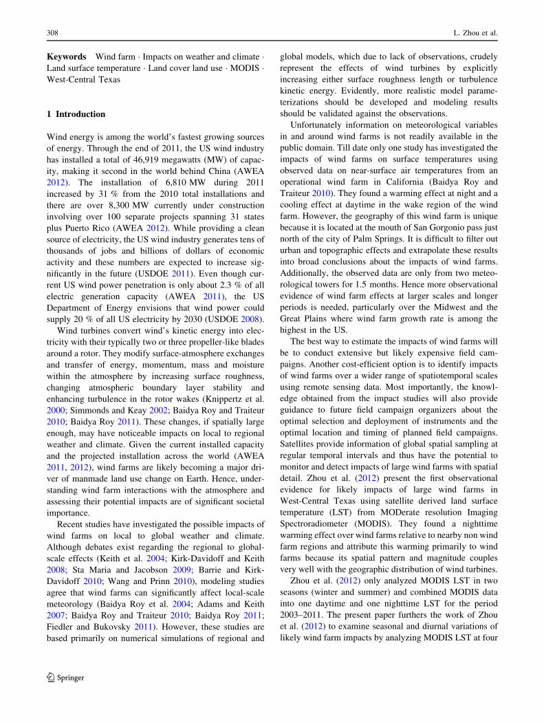
Fig. 1 Histograms of

individual wind turbines built

annually for the period

2001–2011 based on the data

from FAA. The number of

annual (red) and accumulated

(blue) turbines built for each

year is listed on the top of each

bar. The location of the study

region is plotted within the map

of continental US

Diurnal and seasonal variations of wind farm impacts 309

123

nighttime and *10:30 a.m. (Terra) and *1:30 p.m.

(Aqua) during daytime, providing validated, global mea-

surements in large-scale dynamics and processes occurring

on the land, in the oceans, and in the lower atmosphere. For

simplicity, we use local solar time *22:30, *1:30,

*10:30 and *13:30 to denote the acquisition times of the

MODIS LST measurements in this paper.

As LST changes diurnally, we include the MODIS data

from both instruments (Terra and Aqua). Daily LST data

are also available but with many gaps and missing values.

Hence we choose 8-day LST products from Terra

(MOD11A2) and Aqua (MYD11A2) that are averaged

from 2 to 8 days of the daily product (Wan 2002). The

MODIS LST data represent the best quality retrieval pos-

sible from clear-sky conditions over each 8-day period.

Their accuracy has been assessed over a widely distributed

set of locations and time periods via several ground-truth

and validation efforts. Although there may be other

improvements, these data have been used extensively in a

variety of areas and proven to be of high quality. For

example, validation studies in 47 clear-sky cases indicate

that the accuracy of MODIS LST is better than 1 K in most

cases (39 out of 47) and the root of mean squares of dif-

ferences is less than 0.7 K for all 47 cases or 0.5 K for all

but the 8 cases apparently with heavy aerosol loadings

(Wan 2006).

For each year, there are 184 LST images (46 8-day

composites 9 4 times per composite). First, we aggregate

the 8-day MODIS LST data into monthly means from the

8-day composites within each month and then create

monthly anomalies by removing the monthly climatology

for each pixel. Second, we aggregate the monthly means

and anomalies into seasonal ones in DJF (Dec–Jan–Feb),

MAM (Mar–Apr–May), JJA (Jun–Jul–Aug) and SON

(Sep–Oct–Nov). Similarly, annual (referred to as ANN)

means and anomalies are also created. As the Aqua data is

only available starting in July 2002 while Terra has data

starting in March 2000, we have in total 9 years of seasonal

means and anomalies of LST for the period 2003–2011

(note that only the data with a whole year of LST are

considered). Finally for each season in each year, we have

4 images of LST corresponding to the 4 acquisition times

of the MODIS data.

The MODIS data are archived by tile (each tile repre-

sents a 10� by 10� grid cell) in the Sinusoidal equal area

projection, which has a tilt angle of *45� relative to the

local latitude/longitude of our study region. So the MODIS

seasonal mean and anomalies are re-projected into pixels at

0.01� resolution (*1.1 km), which is slightly coarser than

the original MODIS 1 km data to avoid gaps in spatial

interpolation. In total, there are 9,600 pixels (120 col-

umns 9 80 lines) centered around 2,358 wind turbines in

the study region (Fig. 2).

For brevity, we use the following acronyms to represent

two groups of pixels in our study region (Fig. 2c): (1) WFPs

(wind farm pixels, i.e., 890) and (2) NNWFPs (nearby non-

a

b

c

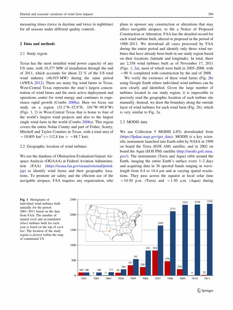
Fig. 2 Geographic locations (latitude and longitude) of wind turbines:

a 2,358 individual turbine sites (plus symbol in red) built in the period

2001–2011 based on the FAA record, b the boundary of wind farms (plus

symbol in red) identified via Google Earth, and c definition of wind farm

pixels (WFPs, in red) and nearby non wind farm pixels (NNWFPs, in

blue) at 0.01� resolution. In b, the outside layer of wind turbines were

drawn in Google Earth as the boundary of wind farms. In c, pixels with at

least one wind turbine are defined as WFPs (in total: 890 pixels) and

those that are between 6 and 9 pixels (4 pixels in width) away from WFPs

are defined as NNWFPs (in total: 1,538 pixels). The pixels between

WFPs and NNWFPs (about 5 pixels between red and blue) are defined as

the transitional zone given the difficulty in objectively defining the

boundary of downwind impacts of wind farms

310 L. Zhou et al.

123

wind-farm pixels, i.e., 1,538). We define the pixels with at

least one wind turbine as WFPs and those that are between 6

and 9 pixels (4 pixels in width) away from WFPs as

NNWFPs. We leave a transitional zone of 5 pixels between

WFPs and NNWFPs given the difficulty in objectively

defining the boundary of downwind pixels (Fig. 2c).

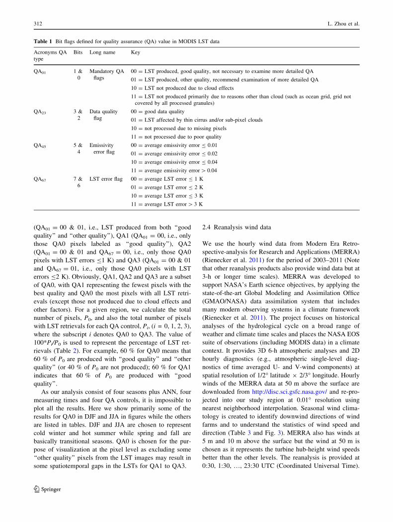
Quality assurance value (QA) fields are attached to the

MODIS LST data (Table 1). QA can tell us whether the

LST is produced (QA01 = 00 or 01) or not (QA01 = 10 or

11, due to cloud effects or other factors). If the LST is

produced, the QA labels it into ‘‘good quality’’

(QA01 = 00) or ‘‘other quality’’ (QA01 = 01). For the LST

produced from ‘‘other quality’’, its average error is pro-

vided (QA67 = 00 for errors B1 K, QA67 = 01 for errors

B2 K, QA67 = 10 for errors B3 K and QA67 = 11 for

errors [3 K).

To assess uncertainties of MODIS LST retrievals to our

results, we consider four different QA controls: QA0

a b

c d

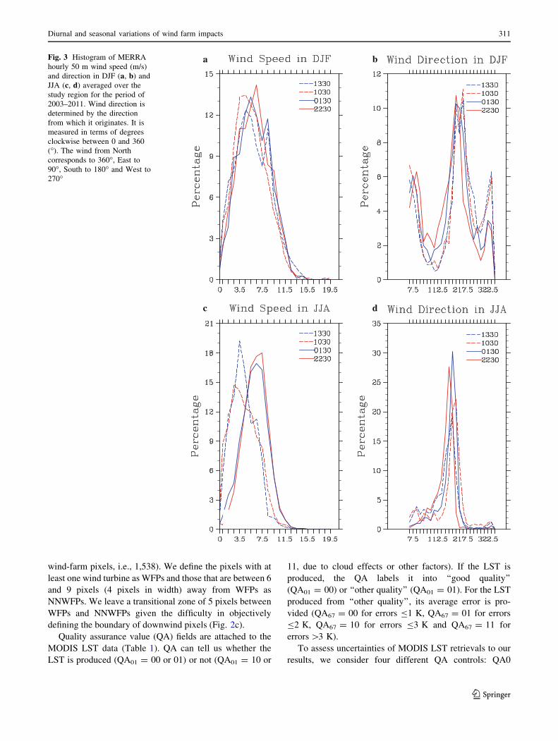
Fig. 3 Histogram of MERRA

hourly 50 m wind speed (m/s)

and direction in DJF (a, b) and

JJA (c, d) averaged over the

study region for the period of

2003–2011. Wind direction is

determined by the direction

from which it originates. It is

measured in terms of degrees

clockwise between 0 and 360

(�). The wind from North

corresponds to 360�, East to

90�, South to 180� and West to

270�

Diurnal and seasonal variations of wind farm impacts 311

123

(QA01 = 00 & 01, i.e., LST produced from both ‘‘good

quality’’ and ‘‘other quality’’), QA1 (QA01 = 00, i.e., only

those QA0 pixels labeled as ‘‘good quality’’), QA2

(QA01 = 00 & 01 and QA67 = 00, i.e., only those QA0

pixels with LST errors B1 K) and QA3 (QA01 = 00 & 01

and QA67 = 01, i.e., only those QA0 pixels with LST

errors B2 K). Obviously, QA1, QA2 and QA3 are a subset

of QA0, with QA1 representing the fewest pixels with the

best quality and QA0 the most pixels with all LST retri-

evals (except those not produced due to cloud effects and

other factors). For a given region, we calculate the total

number of pixels, P0, and also the total number of pixels

with LST retrievals for each QA control, Pi, (i = 0, 1, 2, 3),

where the subscript i denotes QA0 to QA3. The value of

100*Pi/P0 is used to represent the percentage of LST ret-

rievals (Table 2). For example, 60 % for QA0 means that

60 % of P0 are produced with ‘‘good quality’’ and ‘‘other

quality’’ (or 40 % of P0 are not produced); 60 % for QA1

indicates that 60 % of P0 are produced with ‘‘good

quality’’.

As our analysis consist of four seasons plus ANN, four

measuring times and four QA controls, it is impossible to

plot all the results. Here we show primarily some of the

results for QA0 in DJF and JJA in figures while the others

are listed in tables. DJF and JJA are chosen to represent

cold winter and hot summer while spring and fall are

basically transitional seasons. QA0 is chosen for the pur-

pose of visualization at the pixel level as excluding some

‘‘other quality’’ pixels from the LST images may result in

some spatiotemporal gaps in the LSTs for QA1 to QA3.

2.4 Reanalysis wind data

We use the hourly wind data from Modern Era Retro-

spective-analysis for Research and Applications (MERRA)

(Rienecker et al. 2011) for the period of 2003–2011 (Note

that other reanalysis products also provide wind data but at

3-h or longer time scales). MERRA was developed to

support NASA’s Earth science objectives, by applying the

state-of-the-art Global Modeling and Assimilation Office

(GMAO/NASA) data assimilation system that includes

many modern observing systems in a climate framework

(Rienecker et al. 2011). The project focuses on historical

analyses of the hydrological cycle on a broad range of

weather and climate time scales and places the NASA EOS

suite of observations (including MODIS data) in a climate

context. It provides 3D 6-h atmospheric analyses and 2D

hourly diagnostics (e.g., atmospheric single-level diag-

nostics of time averaged U- and V-wind components) at

spatial resolution of 1/2� latitude 9 2/3� longitude. Hourly

winds of the MERRA data at 50 m above the surface are

downloaded from http://disc.sci.gsfc.nasa.gov/ and re-pro-

jected into our study region at 0.01� resolution using

nearest neighborhood interpolation. Seasonal wind clima-

tology is created to identify downwind directions of wind

farms and to understand the statistics of wind speed and

direction (Table 3 and Fig. 3). MERRA also has winds at

5 m and 10 m above the surface but the wind at 50 m is

chosen as it represents the turbine hub-height wind speeds

better than the other levels. The reanalysis is provided at

0:30, 1:30, …, 23:30 UTC (Coordinated Universal Time).

Table 1 Bit flags defined for quality assurance (QA) value in MODIS LST data

Acronyms QA

type

Bits Long name Key

QA01 1 &

0

Mandatory QA

flags

00 = LST produced, good quality, not necessary to examine more detailed QA

01 = LST produced, other quality, recommend examination of more detailed QA

10 = LST not produced due to cloud effects

11 = LST not produced primarily due to reasons other than cloud (such as ocean grid, grid not

covered by all processed granules)

QA23 3 &

2

Data quality

flag

00 = good data quality

01 = LST affected by thin cirrus and/or sub-pixel clouds

10 = not processed due to missing pixels

11 = not processed due to poor quality

QA45 5 &

4

Emissivity

error flag

00 = average emissivity error B 0.01

01 = average emissivity error B 0.02

10 = average emissivity error B 0.04

11 = average emissivity error [ 0.04

QA67 7 &

6

LST error flag 00 = average LST error B 1 K

01 = average LST error B 2 K

10 = average LST error B 3 K

11 = average LST error [ 3 K

312 L. Zhou et al.

123

We use the winds at 04:30, 07:30, 16:30 and 19:30 UTC,

which roughly correspond to the MODIS LSTs at local

solar time *22:30, *1:30, *10:30 and *13:30, for this

analysis.

2.5 Detection and attribution methods

We first discuss the spatiotemporal variability of LST in

the study region and next describe methods used to attri-

bute and quantify the impacts of wind farms on LST.

2.5.1 LST spatiotemporal variability

Besides possible impacts from wind farms, LST variability

over the study region consists of two major components:

(1) temporal variability controlled primarily by regional or

large-scale meteorological conditions and (2) spatial vari-

ability at pixel level that is mostly related to changes in

topography and land surface types. Minimizing such vari-

ability is the key to uncovering wind farm impacts.

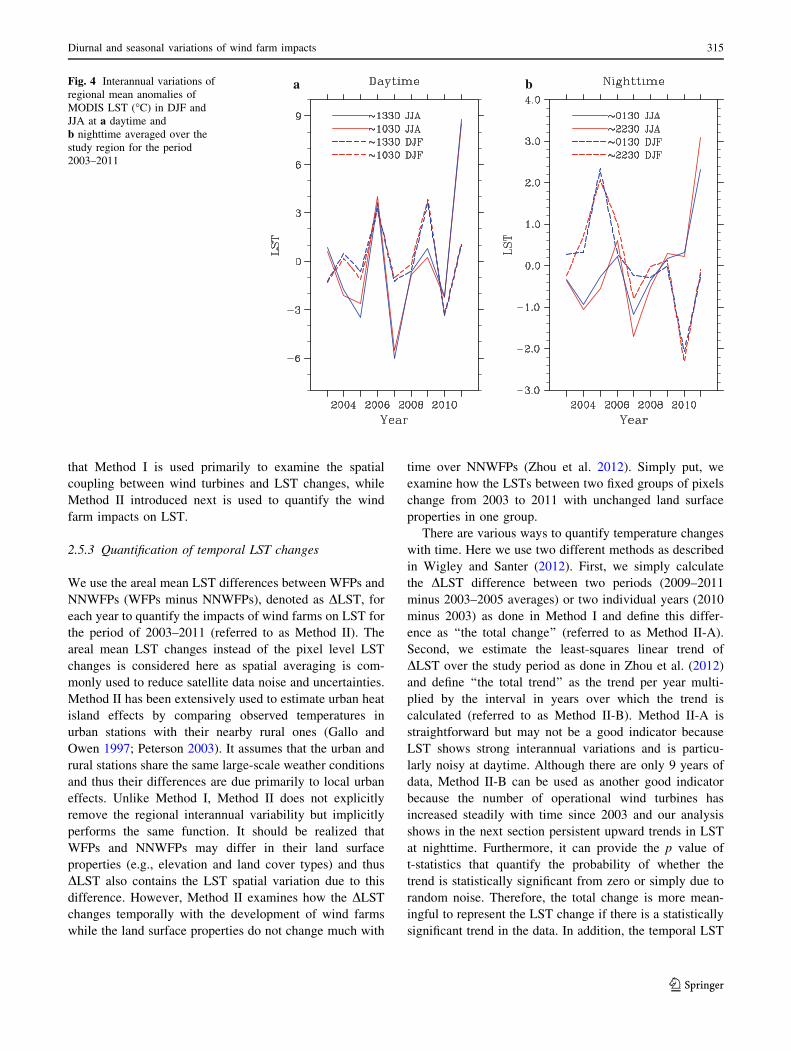
Figure 4 shows interannual variations of regional mean

MODIS LST anomalies in DJF and JJA averaged over the

entire study region for the period 2003–2011. The study

region exhibits a strong interannual variability, particularly

in summer. For example, in JJA, the LST ranges from -6.0

to 8.8 �C (-1.2 to 3.3 �C) at *1:30 (*13:30), with the

coldest year in 2007 and the warmest year in 2011 when the

historic Texas drought occurred (Hylton 2011). The two

measurements at daytime or nighttime generally show

similar LST variations. For each season and each measuring

time, we calculated this regional mean LST anomaly (i.e.,

one value per year from 2003 to 2011) and refer to it as the

‘‘regional interannual variability’’ thereafter.

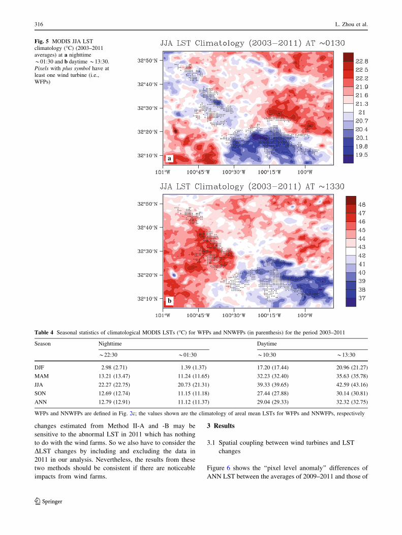
MODIS LST also exhibits strong spatial variability at

pixel level that is mostly related to changes in topography

and land surface types (Zhou et al. 2012). Figure 5 shows

the climatology of JJA LST at *1:30 and *13:30. The

northeastern and southwestern parts of the study region are

generally warmer than the southeastern and northwestern

parts. The LST varies from one wind farm to another,

within WFPs, and between WFPs and NNWFPs. Interest-

ingly, the areal mean LST between WFPs and NNWFPs,

however, is very small (Table 4), indicating the LSTs

averaged over the two regions are very similar.

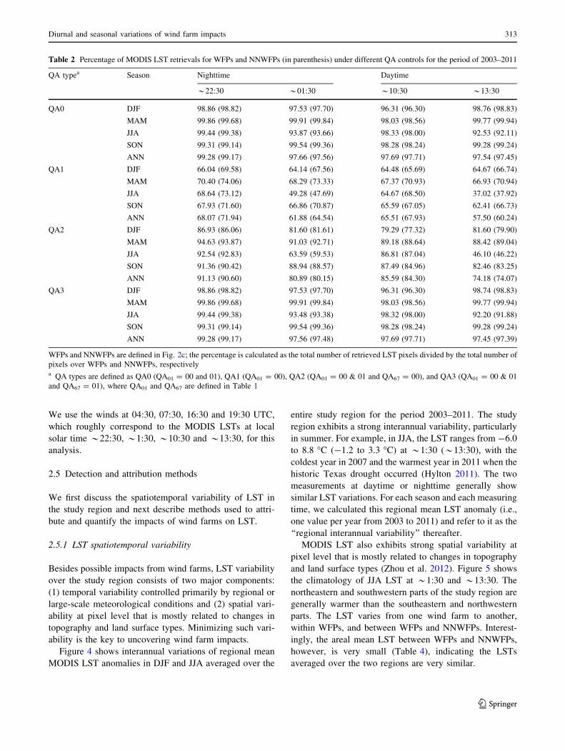
Table 2 Percentage of MODIS LST retrievals for WFPs and NNWFPs (in parenthesis) under different QA controls for the period of 2003–2011

QA typea Season Nighttime Daytime

*22:30 *01:30 *10:30 *13:30

QA0 DJF 98.86 (98.82) 97.53 (97.70) 96.31 (96.30) 98.76 (98.83)

MAM 99.86 (99.68) 99.91 (99.84) 98.03 (98.56) 99.77 (99.94)

JJA 99.44 (99.38) 93.87 (93.66) 98.33 (98.00) 92.53 (92.11)

SON 99.31 (99.14) 99.54 (99.36) 98.28 (98.24) 99.28 (99.24)

ANN 99.28 (99.17) 97.66 (97.56) 97.69 (97.71) 97.54 (97.45)

QA1 DJF 66.04 (69.58) 64.14 (67.56) 64.48 (65.69) 64.67 (66.74)

MAM 70.40 (74.06) 68.29 (73.33) 67.37 (70.93) 66.93 (70.94)

JJA 68.64 (73.12) 49.28 (47.69) 64.67 (68.50) 37.02 (37.92)

SON 67.93 (71.60) 66.86 (70.87) 65.59 (67.05) 62.41 (66.73)

ANN 68.07 (71.94) 61.88 (64.54) 65.51 (67.93) 57.50 (60.24)

QA2 DJF 86.93 (86.06) 81.60 (81.61) 79.29 (77.32) 81.60 (79.90)

MAM 94.63 (93.87) 91.03 (92.71) 89.18 (88.64) 88.42 (89.04)

JJA 92.54 (92.83) 63.59 (59.53) 86.81 (87.04) 46.10 (46.22)

SON 91.36 (90.42) 88.94 (88.57) 87.49 (84.96) 82.46 (83.25)

ANN 91.13 (90.60) 80.89 (80.15) 85.59 (84.30) 74.18 (74.07)

QA3 DJF 98.86 (98.82) 97.53 (97.70) 96.31 (96.30) 98.74 (98.83)

MAM 99.86 (99.68) 99.91 (99.84) 98.03 (98.56) 99.77 (99.94)

JJA 99.44 (99.38) 93.48 (93.38) 98.32 (98.00) 92.20 (91.88)

SON 99.31 (99.14) 99.54 (99.36) 98.28 (98.24) 99.28 (99.24)

ANN 99.28 (99.17) 97.56 (97.48) 97.69 (97.71) 97.45 (97.39)

WFPs and NNWFPs are defined in Fig. 2c; the percentage is calculated as the total number of retrieved LST pixels divided by the total number of

pixels over WFPs and NNWFPs, respectivelya QA types are defined as QA0 (QA01 = 00 and 01), QA1 (QA01 = 00), QA2 (QA01 = 00 & 01 and QA67 = 00), and QA3 (QA01 = 00 & 01

and QA67 = 01), where QA01 and QA67 are defined in Table 1

Diurnal and seasonal variations of wind farm impacts 313

123

As the wind farm impact on LST is likely small in

magnitude, our analysis attempts to isolate this impact

from the background signal by minimizing the influence of

topography, land cover, and regional interannual variations

of weather/climate. Local effects at pixel level due to

spatial variability in topography and land cover can be

minimized through the use of anomalies as done in Sect.

2.3. The strong interannual variability can be minimized by

removing the ‘‘regional interannual variability’’ from the

original LST time series anomalies as introduced next.

2.5.2 Spatial coupling analysis

If the development of wind farms has some impacts on

LST and if such impact is large enough to be detected by

MODIS, the observed MODIS LST change should couple

spatially with the wind turbines. Therefore, we calculate

the LST difference between two periods (or two individual

years) at pixel level, denoted as DLST, and check their

spatial coupling with wind turbines (referred to as Method

I). As wind turbines in the study region were constructed

by stages, with most built in 2005–2008 (Fig. 1), we

choose the first 3 years of data (2003–2005) to represent

the case with the least impacts and the last 3 years

(2009–2011) of data to represent the case with the most

likely impacts. Similarly, we also choose two individual

years, the first year, 2003, and the second last year, 2010, to

quantify the DLST (note that the last year 2011 is not

chosen because of its abnormal LST due to the historic

drought in 2011).

As the DLST also contains the background ‘‘regional

interannual variability’’ signal at these two periods (or

years) that is unrelated to wind farms, we subtract this

signal from the original anomalies for each pixel (referred

to as ‘‘pixel level anomaly’’) to minimize its impact on

DLST (Zhou et al. 2012). Doing so emphasizes the DLST

spatial variability at pixel scale. For example, if a region is

warmer this year than last year but with different warming

rates at different pixels, the DLST (this year’s anomaly

minus last year’s anomaly) will show the warming every-

where, but after removing the regional mean warming rate,

the spatial variability of the warming rate for every pixel

can be easily identified. Note that the ‘‘pixel level anom-

aly’’ represents relative changes, not the absolute changes.

In other words, the resulting warming or cooling rate rep-

resents a change relative to the regional mean value. Note

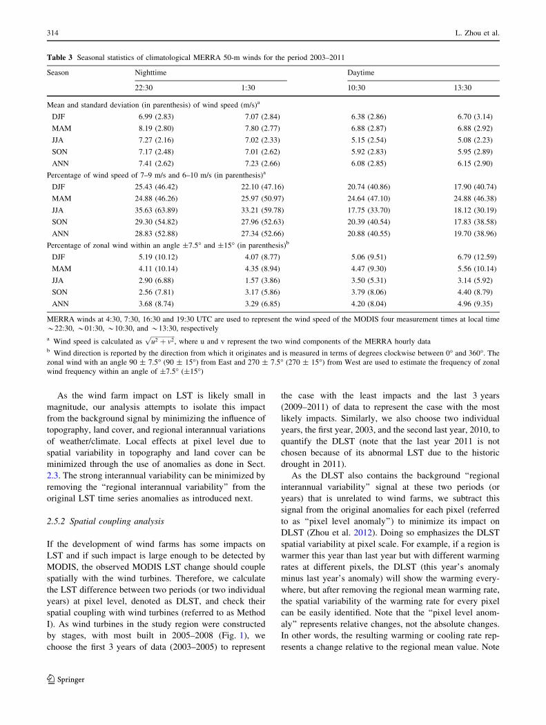
Table 3 Seasonal statistics of climatological MERRA 50-m winds for the period 2003–2011

Season Nighttime Daytime

22:30 1:30 10:30 13:30

Mean and standard deviation (in parenthesis) of wind speed (m/s)a

DJF 6.99 (2.83) 7.07 (2.84) 6.38 (2.86) 6.70 (3.14)

MAM 8.19 (2.80) 7.80 (2.77) 6.88 (2.87) 6.88 (2.92)

JJA 7.27 (2.16) 7.02 (2.33) 5.15 (2.54) 5.08 (2.23)

SON 7.17 (2.48) 7.01 (2.62) 5.92 (2.83) 5.95 (2.89)

ANN 7.41 (2.62) 7.23 (2.66) 6.08 (2.85) 6.15 (2.90)

Percentage of wind speed of 7–9 m/s and 6–10 m/s (in parenthesis)a

DJF 25.43 (46.42) 22.10 (47.16) 20.74 (40.86) 17.90 (40.74)

MAM 24.88 (46.26) 25.97 (50.97) 24.64 (47.10) 24.88 (46.38)

JJA 35.63 (63.89) 33.21 (59.78) 17.75 (33.70) 18.12 (30.19)

SON 29.30 (54.82) 27.96 (52.63) 20.39 (40.54) 17.83 (38.58)

ANN 28.83 (52.88) 27.34 (52.66) 20.88 (40.55) 19.70 (38.96)

Percentage of zonal wind within an angle ±7.5� and ±15� (in parenthesis)b

DJF 5.19 (10.12) 4.07 (8.77) 5.06 (9.51) 6.79 (12.59)

MAM 4.11 (10.14) 4.35 (8.94) 4.47 (9.30) 5.56 (10.14)

JJA 2.90 (6.88) 1.57 (3.86) 3.50 (5.31) 3.14 (5.92)

SON 2.56 (7.81) 3.17 (5.86) 3.79 (8.06) 4.40 (8.79)

ANN 3.68 (8.74) 3.29 (6.85) 4.20 (8.04) 4.96 (9.35)

MERRA winds at 4:30, 7:30, 16:30 and 19:30 UTC are used to represent the wind speed of the MODIS four measurement times at local time

*22:30, *01:30, *10:30, and *13:30, respectively

a Wind speed is calculated asffiffiffiffiffiffiffiffiffiffiffiffiffiffiffi

u2 þ v2p

, where u and v represent the two wind components of the MERRA hourly datab Wind direction is reported by the direction from which it originates and is measured in terms of degrees clockwise between 0� and 360�. The

zonal wind with an angle 90 ± 7.5� (90 ± 15�) from East and 270 ± 7.5� (270 ± 15�) from West are used to estimate the frequency of zonal

wind frequency within an angle of ±7.5� (±15�)

314 L. Zhou et al.

123

that Method I is used primarily to examine the spatial

coupling between wind turbines and LST changes, while

Method II introduced next is used to quantify the wind

farm impacts on LST.

2.5.3 Quantification of temporal LST changes

We use the areal mean LST differences between WFPs and

NNWFPs (WFPs minus NNWFPs), denoted as DLST, for

each year to quantify the impacts of wind farms on LST for

the period of 2003–2011 (referred to as Method II). The

areal mean LST changes instead of the pixel level LST

changes is considered here as spatial averaging is com-

monly used to reduce satellite data noise and uncertainties.

Method II has been extensively used to estimate urban heat

island effects by comparing observed temperatures in

urban stations with their nearby rural ones (Gallo and

Owen 1997; Peterson 2003). It assumes that the urban and

rural stations share the same large-scale weather conditions

and thus their differences are due primarily to local urban

effects. Unlike Method I, Method II does not explicitly

remove the regional interannual variability but implicitly

performs the same function. It should be realized that

WFPs and NNWFPs may differ in their land surface

properties (e.g., elevation and land cover types) and thus

DLST also contains the LST spatial variation due to this

difference. However, Method II examines how the DLST

changes temporally with the development of wind farms

while the land surface properties do not change much with

time over NNWFPs (Zhou et al. 2012). Simply put, we

examine how the LSTs between two fixed groups of pixels

change from 2003 to 2011 with unchanged land surface

properties in one group.

There are various ways to quantify temperature changes

with time. Here we use two different methods as described

in Wigley and Santer (2012). First, we simply calculate

the DLST difference between two periods (2009–2011

minus 2003–2005 averages) or two individual years (2010

minus 2003) as done in Method I and define this differ-

ence as ‘‘the total change’’ (referred to as Method II-A).

Second, we estimate the least-squares linear trend of

DLST over the study period as done in Zhou et al. (2012)

and define ‘‘the total trend’’ as the trend per year multi-

plied by the interval in years over which the trend is

calculated (referred to as Method II-B). Method II-A is

straightforward but may not be a good indicator because

LST shows strong interannual variations and is particu-

larly noisy at daytime. Although there are only 9 years of

data, Method II-B can be used as another good indicator

because the number of operational wind turbines has

increased steadily with time since 2003 and our analysis

shows in the next section persistent upward trends in LST

at nighttime. Furthermore, it can provide the p value of

t-statistics that quantify the probability of whether the

trend is statistically significant from zero or simply due to

random noise. Therefore, the total change is more mean-

ingful to represent the LST change if there is a statistically

significant trend in the data. In addition, the temporal LST

a bFig. 4 Interannual variations of

regional mean anomalies of

MODIS LST (�C) in DJF and

JJA at a daytime and

b nighttime averaged over the

study region for the period

2003–2011

Diurnal and seasonal variations of wind farm impacts 315

123

changes estimated from Method II-A and -B may be

sensitive to the abnormal LST in 2011 which has nothing

to do with the wind farms. So we also have to consider the

DLST changes by including and excluding the data in

2011 in our analysis. Nevertheless, the results from these

two methods should be consistent if there are noticeable

impacts from wind farms.

3 Results

3.1 Spatial coupling between wind turbines and LST

changes

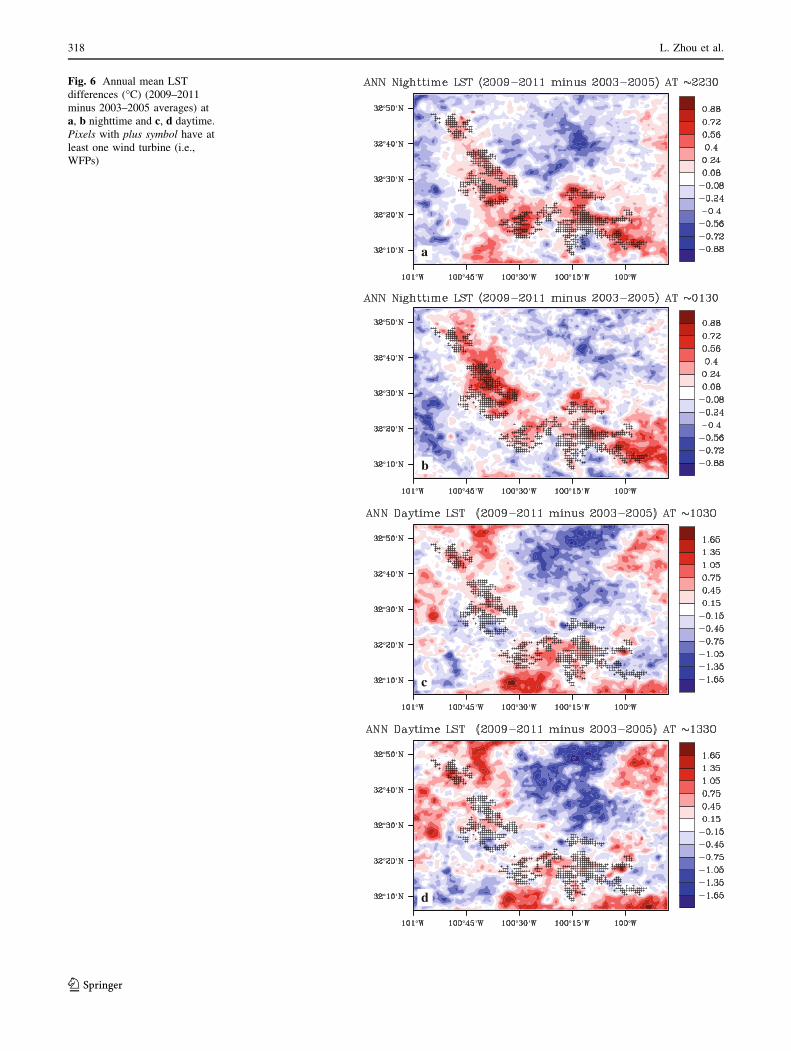
Figure 6 shows the ‘‘pixel level anomaly’’ differences of

ANN LST between the averages of 2009–2011 and those of

a

b

Fig. 5 MODIS JJA LST

climatology (�C) (2003–2011

averages) at a nighttime

*01:30 and b daytime *13:30.

Pixels with plus symbol have at

least one wind turbine (i.e.,

WFPs)

Table 4 Seasonal statistics of climatological MODIS LSTs (�C) for WFPs and NNWFPs (in parenthesis) for the period 2003–2011

Season Nighttime Daytime

*22:30 *01:30 *10:30 *13:30

DJF 2.98 (2.71) 1.39 (1.37) 17.20 (17.44) 20.96 (21.27)

MAM 13.21 (13.47) 11.24 (11.65) 32.23 (32.40) 35.63 (35.78)

JJA 22.27 (22.75) 20.73 (21.31) 39.33 (39.65) 42.59 (43.16)

SON 12.69 (12.74) 11.15 (11.18) 27.44 (27.88) 30.14 (30.81)

ANN 12.79 (12.91) 11.12 (11.37) 29.04 (29.33) 32.32 (32.75)

WFPs and NNWFPs are defined in Fig. 2c; the values shown are the climatology of areal mean LSTs for WFPs and NNWFPs, respectively

316 L. Zhou et al.

123

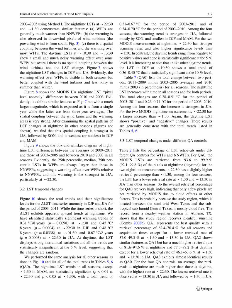
2003–2005 using Method I. The nighttime LSTs at *22:30

and *1:30 demonstrate similar features: (a) WFPs are

generally much warmer than NNWFPs; (b) the warming is

also observed in downwind pixels of wind turbines (the

prevailing wind is from south, Fig. 3); (c) there is a spatial

coupling between the wind turbines and the warming over

most WFPs. The daytime LSTs at *10:30 and *13:30

show a small and much noisy warming effect over some

WFPs but overall there is no spatial coupling between the

wind turbines and the LST change. Figure 7 shows

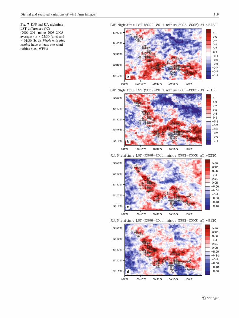
the nighttime LST changes in DJF and JJA. Evidently, the

warming effect over WFPs is visible in both seasons but

better coupled with the wind turbines and less noisy in

summer than winter.

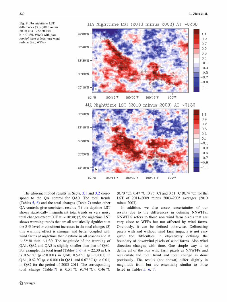
Figure 8 shows the MODIS JJA nighttime LST ‘‘pixel

level anomaly’’ differences between 2010 and 2003. Evi-

dently, it exhibits similar features as Fig. 7 but with a much

larger magnitude, which is expected as it is from a single

year while the latter are from three-year averages. The

spatial coupling between the wind farms and the warming

areas is very strong. After examining the spatial patterns of

LST changes at nighttime in other seasons (figures not

shown), we find that this spatial coupling is strongest in

JJA, followed by SON, and is weakest (or noisiest) in DJF

and MAM.

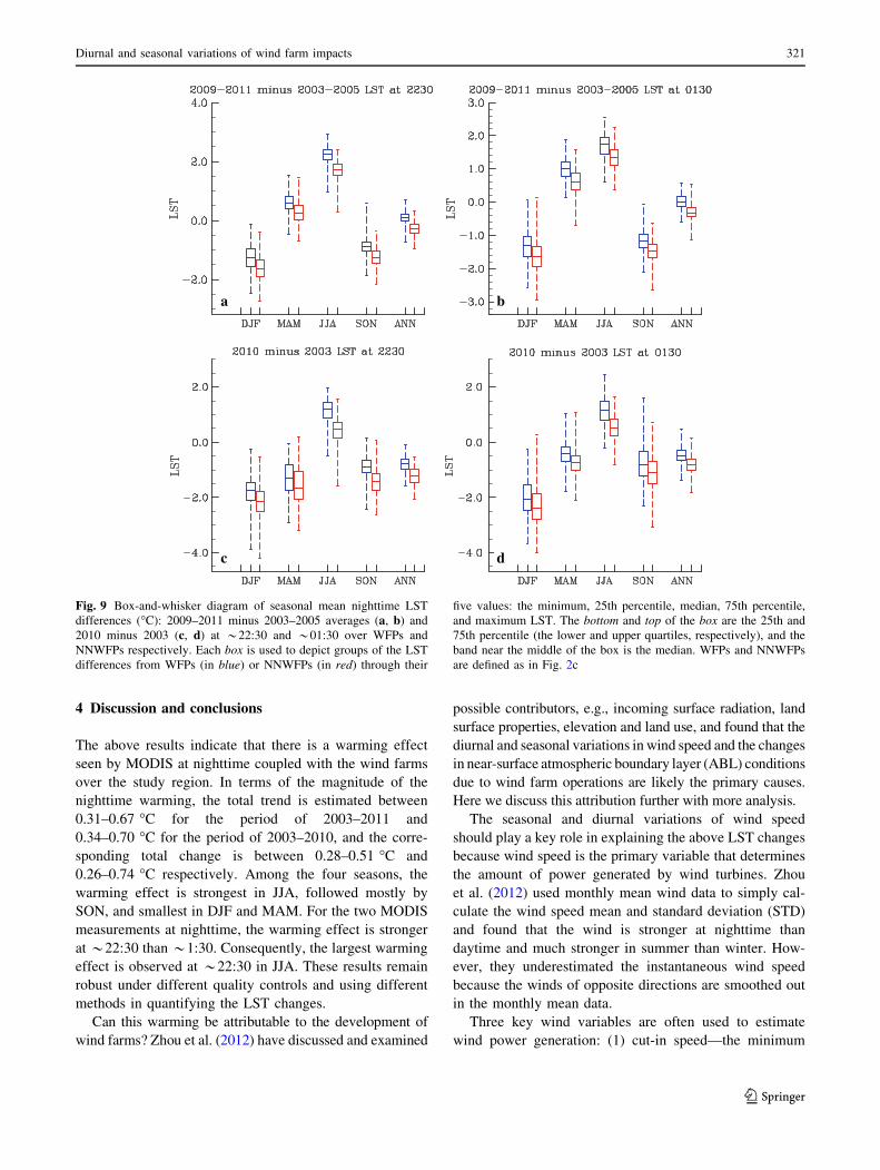
Figure 9 shows the box-and-whisker diagram of night-

time LST differences between the averages of 2009–2011

and those of 2003–2005 and between 2010 and 2003 in all

seasons. Evidently, the 25th percentile, median, 75th per-

centile LSTs in WFPs are always larger than those in

NNWFPs, suggesting a warming effect over WFPs relative

to NNWFPs, and this warming is the strongest in JJA,

particularly at *22:30.

3.2 LST temporal changes

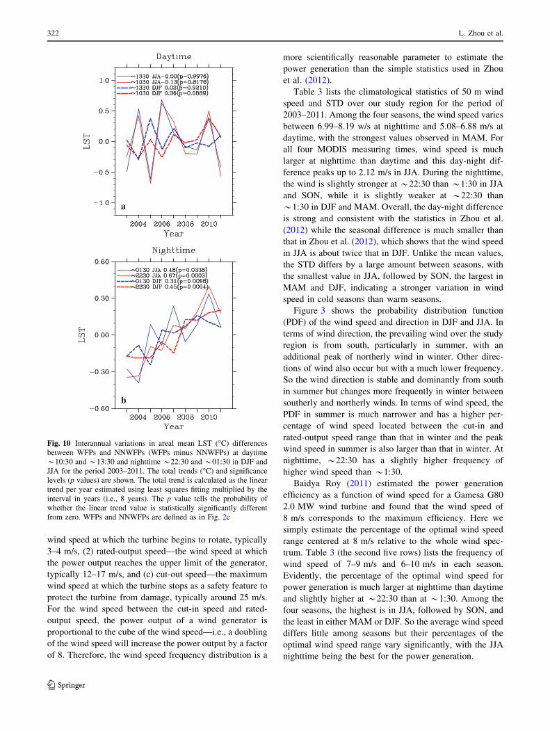
Figure 10 shows the total trends and their significance

levels for the DLST time series anomaly in DJF and JJA for

the period of 2003–2011. While the time series is short, the

DLST exhibits apparent upward trends at nighttime. We

have identified statistically significant warming trends of

0.31 �C/8 years (p = 0.0098) at *1:30 and 0.45 �C/

8 years (p = 0.0004) at *22:30 in DJF and 0.48 �C/

8 years (p = 0.0338) at *01:30 and 0.67 �C/8 years

(p = 0.0003) at *22:30 in JJA. At daytime, the LST

displays strong interannual variations and all the trends are

statistically insignificant at the 5 % level, suggesting that

the changes are random.

We performed the same analysis for all other seasons as

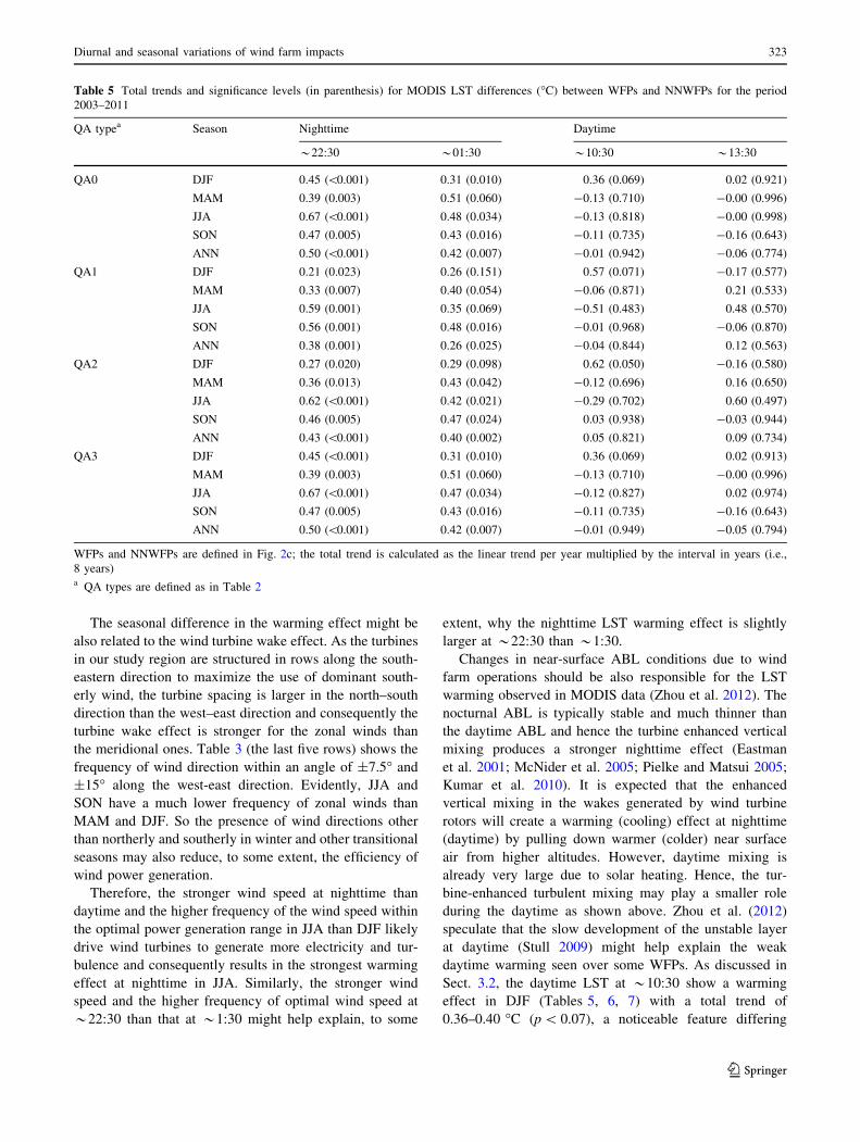
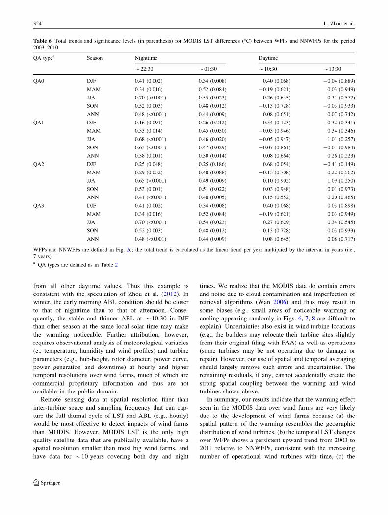
done in Fig. 10 and list all of the total trends in Tables 5, 6

(QA0). The nighttime LST trends in all seasons, except

*1:30 in MAM, are statistically significant (p \ 0.01 at

*22:30 and p \ 0.05 at *1:30), with a total trend of

0.31–0.67 �C for the period of 2003–2011 and of

0.34–0.70 �C for the period of 2003–2010. Among the four

seasons, the warming trend is strongest in JJA, followed

mostly by SON, and smallest in DJF and MAM. For the two

MODIS measurements at nighttime, *22:30 has stronger

warming rates and also higher significance levels than

*1:30. In contrast, the daytime trends range from negative to

positive values and none is statistically significant at the 5 %

level. It is interesting to note that unlike other daytime trends,

the LST in DJF at *10:30 shows a total trend of

0.36–0.40 �C that is statistically significant at the 10 % level.

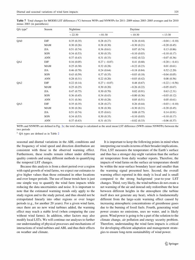
Table 7 (QA0) lists the total change between two peri-

ods: 2011–2009 minus 2003–2005 averages and 2010

minus 2003 (in parenthesis) for all seasons. The nighttime

LST increases with time in all seasons and for both periods.

The total changes are 0.28–0.51 �C for the period of

2003–2011 and 0.26–0.74 �C for the period of 2003–2010.

Among the four seasons, the increase is strongest in JJA.

For the two MODIS nighttime measurements, *22:30 has

a larger increase than *1:30. Again, the daytime LST

shows ‘‘positive’’ and ‘‘negative’’ changes. These results

are generally consistent with the total trends listed in

Tables 5, 6.

3.3 LST temporal changes under different QA controls

Table 2 lists the percentage of LST retrievals under dif-

ferent QA controls for WFPs and NNWFPs. For QA0, the

MODIS LSTs are retrieved from 93.6 to 99.9 %

(92.1–99.8 %) of the pixels at nighttime (daytime); for the

two nighttime measurements, *22:30 has a slightly higher

retrieval percentage than *1:30; among the four seasons,

the LST has a lower retrieval rate at *1:30 and *13:30 in

JJA than other seasons. So the overall retrieval percentage

for QA0 are very high, indicating that only a few pixels are

not retrieved by MODIS due to cloud effects or other

factors. This is probably because the study region, which is

located between the semi-arid West Texas and the sub-

tropical sub-humid Central Texas, is mostly cloud free. The

record from a nearby weather station in Abilene, TX,

shows that the study region receives plentiful sunshine

(Combs 2008b). QA1 represents the best quality with a

retrieval percentage of 62.4–70.4 % for all seasons and

acquisition times except for a lower retrieval rate of

37.0–49.3 % at *1:30 and *13:30 in JJA. QA2 shows

similar features as QA1 but has a much higher retrieval rate

of 81.6–94.6 % at nighttime and 77.3–89.2 % at daytime

except for a lower retrieval rate of 46.1–63.6 % at *1:30

and *13:30 in JJA. QA3 exhibits almost identical results

as QA0. For the four QA controls, on average, the retri-

evals at nighttime are much higher than those at daytime,

with the highest rate at *22:30. The lowest retrieval rate is

observed at *13:30 in JJA and followed by *1:30 in JJA.

Diurnal and seasonal variations of wind farm impacts 317

123

a

b

c

d

Fig. 6 Annual mean LST

differences (�C) (2009–2011

minus 2003–2005 averages) at

a, b nighttime and c, d daytime.

Pixels with plus symbol have at

least one wind turbine (i.e.,

WFPs)

318 L. Zhou et al.

123

a

b

c

d

Fig. 7 DJF and JJA nighttime

LST differences (�C)

(2009–2011 minus 2003–2005

averages) at *22:30 (a, c) and

*01:30 (b, d). Pixels with plus

symbol have at least one wind

turbine (i.e., WFPs)

Diurnal and seasonal variations of wind farm impacts 319

123

The aforementioned results in Sects. 3.1 and 3.2 corre-

spond to the QA control for QA0. The total trends

(Tables 5, 6) and the total changes (Table 7) under other

QA controls give consistent results: (1) the daytime LST

shows statistically insignificant total trends or very noisy

total changes except DJF at *10:30; (2) the nighttime LST

shows warming trends that are all statistically significant at

the 5 % level or consistent increases in the total change; (3)

this warming effect is stronger and better coupled with

wind farms at nighttime than daytime in all seasons and at

*22:30 than *1:30. The magnitude of the warming of

QA1, QA2 and QA3 is slightly smaller than that of QA0.

For example, the total trend (Tables 5, 6) at *22:30 in JJA

is 0.67 �C (p \ 0.001) in QA0, 0.59 �C (p = 0.001) in

QA1, 0.62 �C (p \ 0.001) in QA1, and 0.67 �C (p \ 0.01)

in QA2 for the period of 2003–2011. The corresponding

total change (Table 7) is 0.51 �C (0.74 �C), 0.46 �C

(0.70 �C), 0.47 �C (0.75 �C) and 0.51 �C (0.74 �C) for the

LST of 2011–2009 minus 2003–2005 averages (2010

minus 2003).

In addition, we also assess uncertainties of our

results due to the differences in defining NNWFPs.

NNWFPS refers to those non wind farm pixels that are

very close to WFPs but not affected by wind farms.

Obviously, it can be defined otherwise. Delineating

pixels with and without wind farm impacts is not easy

given the difficulties in objectively defining the

boundary of downwind pixels of wind farms. Also wind

direction changes with time. One simple way is to

define all of the non wind farm pixels as NNWFPs and

recalculate the total trend and total change as done

previously. The results (not shown) differ slightly in

magnitude from but are essentially similar to those

listed in Tables 5, 6, 7.

a

b

Fig. 8 JJA nighttime LST

differences (�C) (2010 minus

2003) at a *22:30 and

b *01:30. Pixels with plus

symbol have at least one wind

turbine (i.e., WFPs)

320 L. Zhou et al.

123

4 Discussion and conclusions

The above results indicate that there is a warming effect

seen by MODIS at nighttime coupled with the wind farms

over the study region. In terms of the magnitude of the

nighttime warming, the total trend is estimated between

0.31–0.67 �C for the period of 2003–2011 and

0.34–0.70 �C for the period of 2003–2010, and the corre-

sponding total change is between 0.28–0.51 �C and

0.26–0.74 �C respectively. Among the four seasons, the

warming effect is strongest in JJA, followed mostly by

SON, and smallest in DJF and MAM. For the two MODIS

measurements at nighttime, the warming effect is stronger

at *22:30 than *1:30. Consequently, the largest warming

effect is observed at *22:30 in JJA. These results remain

robust under different quality controls and using different

methods in quantifying the LST changes.

Can this warming be attributable to the development of

wind farms? Zhou et al. (2012) have discussed and examined

possible contributors, e.g., incoming surface radiation, land

surface properties, elevation and land use, and found that the

diurnal and seasonal variations in wind speed and the changes

in near-surface atmospheric boundary layer (ABL) conditions

due to wind farm operations are likely the primary causes.

Here we discuss this attribution further with more analysis.

The seasonal and diurnal variations of wind speed

should play a key role in explaining the above LST changes

because wind speed is the primary variable that determines

the amount of power generated by wind turbines. Zhou

et al. (2012) used monthly mean wind data to simply cal-

culate the wind speed mean and standard deviation (STD)

and found that the wind is stronger at nighttime than

daytime and much stronger in summer than winter. How-

ever, they underestimated the instantaneous wind speed

because the winds of opposite directions are smoothed out

in the monthly mean data.

Three key wind variables are often used to estimate

wind power generation: (1) cut-in speed—the minimum

a b

c d

Fig. 9 Box-and-whisker diagram of seasonal mean nighttime LST

differences (�C): 2009–2011 minus 2003–2005 averages (a, b) and

2010 minus 2003 (c, d) at *22:30 and *01:30 over WFPs and

NNWFPs respectively. Each box is used to depict groups of the LST

differences from WFPs (in blue) or NNWFPs (in red) through their

five values: the minimum, 25th percentile, median, 75th percentile,

and maximum LST. The bottom and top of the box are the 25th and

75th percentile (the lower and upper quartiles, respectively), and the

band near the middle of the box is the median. WFPs and NNWFPs

are defined as in Fig. 2c

Diurnal and seasonal variations of wind farm impacts 321

123

wind speed at which the turbine begins to rotate, typically

3–4 m/s, (2) rated-output speed—the wind speed at which

the power output reaches the upper limit of the generator,

typically 12–17 m/s, and (c) cut-out speed—the maximum

wind speed at which the turbine stops as a safety feature to

protect the turbine from damage, typically around 25 m/s.

For the wind speed between the cut-in speed and rated-

output speed, the power output of a wind generator is

proportional to the cube of the wind speed—i.e., a doubling

of the wind speed will increase the power output by a factor

of 8. Therefore, the wind speed frequency distribution is a

more scientifically reasonable parameter to estimate the

power generation than the simple statistics used in Zhou

et al. (2012).

Table 3 lists the climatological statistics of 50 m wind

speed and STD over our study region for the period of

2003–2011. Among the four seasons, the wind speed varies

between 6.99–8.19 w/s at nighttime and 5.08–6.88 m/s at

daytime, with the strongest values observed in MAM. For

all four MODIS measuring times, wind speed is much

larger at nighttime than daytime and this day-night dif-

ference peaks up to 2.12 m/s in JJA. During the nighttime,

the wind is slightly stronger at *22:30 than *1:30 in JJA

and SON, while it is slightly weaker at *22:30 than

*1:30 in DJF and MAM. Overall, the day-night difference

is strong and consistent with the statistics in Zhou et al.

(2012) while the seasonal difference is much smaller than

that in Zhou et al. (2012), which shows that the wind speed

in JJA is about twice that in DJF. Unlike the mean values,

the STD differs by a large amount between seasons, with

the smallest value in JJA, followed by SON, the largest in

MAM and DJF, indicating a stronger variation in wind

speed in cold seasons than warm seasons.

Figure 3 shows the probability distribution function

(PDF) of the wind speed and direction in DJF and JJA. In

terms of wind direction, the prevailing wind over the study

region is from south, particularly in summer, with an

additional peak of northerly wind in winter. Other direc-

tions of wind also occur but with a much lower frequency.

So the wind direction is stable and dominantly from south

in summer but changes more frequently in winter between

southerly and northerly winds. In terms of wind speed, the

PDF in summer is much narrower and has a higher per-

centage of wind speed located between the cut-in and

rated-output speed range than that in winter and the peak

wind speed in summer is also larger than that in winter. At

nighttime, *22:30 has a slightly higher frequency of

higher wind speed than *1:30.

Baidya Roy (2011) estimated the power generation

efficiency as a function of wind speed for a Gamesa G80

2.0 MW wind turbine and found that the wind speed of

8 m/s corresponds to the maximum efficiency. Here we

simply estimate the percentage of the optimal wind speed

range centered at 8 m/s relative to the whole wind spec-

trum. Table 3 (the second five rows) lists the frequency of

wind speed of 7–9 m/s and 6–10 m/s in each season.

Evidently, the percentage of the optimal wind speed for

power generation is much larger at nighttime than daytime

and slightly higher at *22:30 than at *1:30. Among the

four seasons, the highest is in JJA, followed by SON, and

the least in either MAM or DJF. So the average wind speed

differs little among seasons but their percentages of the

optimal wind speed range vary significantly, with the JJA

nighttime being the best for the power generation.

a

b

Fig. 10 Interannual variations in areal mean LST (�C) differences

between WFPs and NNWFPs (WFPs minus NNWFPs) at daytime

*10:30 and *13:30 and nighttime *22:30 and *01:30 in DJF and

JJA for the period 2003–2011. The total trends (�C) and significance

levels (p values) are shown. The total trend is calculated as the linear

trend per year estimated using least squares fitting multiplied by the

interval in years (i.e., 8 years). The p value tells the probability of

whether the linear trend value is statistically significantly different

from zero. WFPs and NNWFPs are defined as in Fig. 2c

322 L. Zhou et al.

123

The seasonal difference in the warming effect might be

also related to the wind turbine wake effect. As the turbines

in our study region are structured in rows along the south-

eastern direction to maximize the use of dominant south-

erly wind, the turbine spacing is larger in the north–south

direction than the west–east direction and consequently the

turbine wake effect is stronger for the zonal winds than

the meridional ones. Table 3 (the last five rows) shows the

frequency of wind direction within an angle of ±7.5� and

±15� along the west-east direction. Evidently, JJA and

SON have a much lower frequency of zonal winds than

MAM and DJF. So the presence of wind directions other

than northerly and southerly in winter and other transitional

seasons may also reduce, to some extent, the efficiency of

wind power generation.

Therefore, the stronger wind speed at nighttime than

daytime and the higher frequency of the wind speed within

the optimal power generation range in JJA than DJF likely

drive wind turbines to generate more electricity and tur-

bulence and consequently results in the strongest warming

effect at nighttime in JJA. Similarly, the stronger wind

speed and the higher frequency of optimal wind speed at

*22:30 than that at *1:30 might help explain, to some

extent, why the nighttime LST warming effect is slightly

larger at *22:30 than *1:30.

Changes in near-surface ABL conditions due to wind

farm operations should be also responsible for the LST

warming observed in MODIS data (Zhou et al. 2012). The

nocturnal ABL is typically stable and much thinner than

the daytime ABL and hence the turbine enhanced vertical

mixing produces a stronger nighttime effect (Eastman

et al. 2001; McNider et al. 2005; Pielke and Matsui 2005;

Kumar et al. 2010). It is expected that the enhanced

vertical mixing in the wakes generated by wind turbine

rotors will create a warming (cooling) effect at nighttime

(daytime) by pulling down warmer (colder) near surface

air from higher altitudes. However, daytime mixing is

already very large due to solar heating. Hence, the tur-

bine-enhanced turbulent mixing may play a smaller role

during the daytime as shown above. Zhou et al. (2012)

speculate that the slow development of the unstable layer

at daytime (Stull 2009) might help explain the weak

daytime warming seen over some WFPs. As discussed in

Sect. 3.2, the daytime LST at *10:30 show a warming

effect in DJF (Tables 5, 6, 7) with a total trend of

0.36–0.40 �C (p \ 0.07), a noticeable feature differing

Table 5 Total trends and significance levels (in parenthesis) for MODIS LST differences (�C) between WFPs and NNWFPs for the period

2003–2011

QA typea Season Nighttime Daytime

*22:30 *01:30 *10:30 *13:30

QA0 DJF 0.45 (\0.001) 0.31 (0.010) 0.36 (0.069) 0.02 (0.921)

MAM 0.39 (0.003) 0.51 (0.060) -0.13 (0.710) -0.00 (0.996)

JJA 0.67 (\0.001) 0.48 (0.034) -0.13 (0.818) -0.00 (0.998)

SON 0.47 (0.005) 0.43 (0.016) -0.11 (0.735) -0.16 (0.643)

ANN 0.50 (\0.001) 0.42 (0.007) -0.01 (0.942) -0.06 (0.774)

QA1 DJF 0.21 (0.023) 0.26 (0.151) 0.57 (0.071) -0.17 (0.577)

MAM 0.33 (0.007) 0.40 (0.054) -0.06 (0.871) 0.21 (0.533)

JJA 0.59 (0.001) 0.35 (0.069) -0.51 (0.483) 0.48 (0.570)

SON 0.56 (0.001) 0.48 (0.016) -0.01 (0.968) -0.06 (0.870)

ANN 0.38 (0.001) 0.26 (0.025) -0.04 (0.844) 0.12 (0.563)

QA2 DJF 0.27 (0.020) 0.29 (0.098) 0.62 (0.050) -0.16 (0.580)

MAM 0.36 (0.013) 0.43 (0.042) -0.12 (0.696) 0.16 (0.650)

JJA 0.62 (\0.001) 0.42 (0.021) -0.29 (0.702) 0.60 (0.497)

SON 0.46 (0.005) 0.47 (0.024) 0.03 (0.938) -0.03 (0.944)

ANN 0.43 (\0.001) 0.40 (0.002) 0.05 (0.821) 0.09 (0.734)

QA3 DJF 0.45 (\0.001) 0.31 (0.010) 0.36 (0.069) 0.02 (0.913)

MAM 0.39 (0.003) 0.51 (0.060) -0.13 (0.710) -0.00 (0.996)

JJA 0.67 (\0.001) 0.47 (0.034) -0.12 (0.827) 0.02 (0.974)

SON 0.47 (0.005) 0.43 (0.016) -0.11 (0.735) -0.16 (0.643)

ANN 0.50 (\0.001) 0.42 (0.007) -0.01 (0.949) -0.05 (0.794)

WFPs and NNWFPs are defined in Fig. 2c; the total trend is calculated as the linear trend per year multiplied by the interval in years (i.e.,

8 years)a QA types are defined as in Table 2

Diurnal and seasonal variations of wind farm impacts 323

123

from all other daytime values. Thus this example is

consistent with the speculation of Zhou et al. (2012). In

winter, the early morning ABL condition should be closer

to that of nighttime than to that of afternoon. Conse-

quently, the stable and thinner ABL at *10:30 in DJF

than other season at the same local solar time may make

the warming noticeable. Further attribution, however,

requires observational analysis of meteorological variables

(e., temperature, humidity and wind profiles) and turbine

parameters (e.g., hub-height, rotor diameter, power curve,

power generation and downtime) at hourly and higher

temporal resolutions over wind farms, much of which are

commercial proprietary information and thus are not

available in the public domain.

Remote sensing data at spatial resolution finer than

inter-turbine space and sampling frequency that can cap-

ture the full diurnal cycle of LST and ABL (e.g., hourly)

would be most effective to detect impacts of wind farms

than MODIS. However, MODIS LST is the only high

quality satellite data that are publically available, have a

spatial resolution smaller than most big wind farms, and

have data for *10 years covering both day and night

times. We realize that the MODIS data do contain errors

and noise due to cloud contamination and imperfection of

retrieval algorithms (Wan 2006) and thus may result in

some biases (e.g., small areas of noticeable warming or

cooling appearing randomly in Figs. 6, 7, 8 are difficult to

explain). Uncertainties also exist in wind turbine locations

(e.g., the builders may relocate their turbine sites slightly

from their original filing with FAA) as well as operations

(some turbines may be not operating due to damage or

repair). However, our use of spatial and temporal averaging

should largely remove such errors and uncertainties. The

remaining residuals, if any, cannot accidentally create the

strong spatial coupling between the warming and wind

turbines shown above.

In summary, our results indicate that the warming effect

seen in the MODIS data over wind farms are very likely

due to the development of wind farms because (a) the

spatial pattern of the warming resembles the geographic

distribution of wind turbines, (b) the temporal LST changes

over WFPs shows a persistent upward trend from 2003 to

2011 relative to NNWFPs, consistent with the increasing

number of operational wind turbines with time, (c) the

Table 6 Total trends and significance levels (in parenthesis) for MODIS LST differences (�C) between WFPs and NNWFPs for the period

2003–2010

QA typea Season Nighttime Daytime

*22:30 *01:30 *10:30 *13:30

QA0 DJF 0.41 (0.002) 0.34 (0.008) 0.40 (0.068) -0.04 (0.889)

MAM 0.34 (0.016) 0.52 (0.084) -0.19 (0.621) 0.03 (0.949)

JJA 0.70 (\0.001) 0.55 (0.023) 0.26 (0.635) 0.31 (0.577)

SON 0.52 (0.003) 0.48 (0.012) -0.13 (0.728) -0.03 (0.933)

ANN 0.48 (\0.001) 0.44 (0.009) 0.08 (0.651) 0.07 (0.742)

QA1 DJF 0.16 (0.091) 0.26 (0.212) 0.54 (0.123) -0.32 (0.341)

MAM 0.33 (0.014) 0.45 (0.050) -0.03 (0.946) 0.34 (0.346)

JJA 0.68 (\0.001) 0.46 (0.020) -0.05 (0.947) 1.01 (0.257)

SON 0.63 (\0.001) 0.47 (0.029) -0.07 (0.861) -0.01 (0.984)

ANN 0.38 (0.001) 0.30 (0.014) 0.08 (0.664) 0.26 (0.223)

QA2 DJF 0.25 (0.048) 0.25 (0.186) 0.68 (0.054) -0.41 (0.149)

MAM 0.29 (0.052) 0.40 (0.088) -0.13 (0.708) 0.22 (0.562)

JJA 0.65 (\0.001) 0.49 (0.009) 0.10 (0.902) 1.09 (0.250)

SON 0.53 (0.001) 0.51 (0.022) 0.03 (0.948) 0.01 (0.973)

ANN 0.41 (\0.001) 0.40 (0.005) 0.15 (0.552) 0.20 (0.465)

QA3 DJF 0.41 (0.002) 0.34 (0.008) 0.40 (0.068) -0.03 (0.898)

MAM 0.34 (0.016) 0.52 (0.084) -0.19 (0.621) 0.03 (0.949)

JJA 0.70 (\0.001) 0.54 (0.023) 0.27 (0.629) 0.34 (0.545)

SON 0.52 (0.003) 0.48 (0.012) -0.13 (0.728) -0.03 (0.933)

ANN 0.48 (\0.001) 0.44 (0.009) 0.08 (0.645) 0.08 (0.717)

WFPs and NNWFPs are defined in Fig. 2c; the total trend is calculated as the linear trend per year multiplied by the interval in years (i.e.,

7 years)a QA types are defined as in Table 2

324 L. Zhou et al.

123

seasonal and diurnal variations in the ABL conditions and

the frequency of wind speed and direction distribution are

consistent with those in the observed warming effect.

Furthermore, these results remain robust under different

quality controls and using different methods in quantifying

the temporal LST changes.

Because this analysis is from a short period over a region

with rapid growth of wind farms, we expect our estimates to

give higher values than those estimated in other locations

and over longer periods. The use of linear trends here is just

one simple way to quantify the wind farm impacts while

reducing the data uncertainties and noise. It is important to

note that the estimated warming trends only apply to the

study region and to the study period, and thus should not be

extrapolated linearly into other regions or over longer

periods (e.g., for another 20 years). For a given wind farm,

once there are no new wind turbines added, the warming

effect may reach a stable level (when comparing the case

without wind farms). In addition, other factors may also

modify local LSTs. We will continue our analyses to further

our understanding of physical processes and mechanisms of

interactions of wind turbines and ABL and thus their effects

on weather and climate.

It is important to keep the following points in mind when

interpreting our results in terms of their broader implications.

First, LST measures the temperature of the Earth’s surface

and thus has a stronger day-night variation than the surface

air temperature from daily weather reports. Therefore, the

impacts of wind farms on the surface air temperature should

be within the near-surface boundary layer and smaller than

the warming signal presented here. Second, the overall

warming effect reported in this study is local and is small

compared to the strong background year-to-year LST

changes. Third, very likely, the wind turbines do not create a

net warming of the air and instead only redistribute the heat

between different heights in the atmosphere (the turbine

itself does not generate any heat), which is fundamentally

different from the large-scale warming effect caused by

increasing atmospheric concentrations of greenhouse gases

due to the burning of fossil fuels. Fourth, generating wind

power creates no emissions, uses no water, and is likely

green. Wind power is going to be a part of the solution to the

climate change, air pollution and energy security problem.

Therefore, understanding the wind farm impacts is critical

for developing efficient adaptation and management strate-

gies to ensure long-term sustainability of wind power.

Table 7 Total changes for MODIS LST differences (�C) between WFPs and NNWFPs for 2011–2009 minus 2003–2005 averages and for 2010

minus 2003 (in parenthesis)

QA typea Season Nighttime Daytime

*22:30 *01:30 *10:30 *13:30

QA0 DJF 0.35 (0.35) 0.28 (0.27) 0.26 (0.44) -0.04 (-0.10)

MAM 0.30 (0.26) 0.38 (0.30) -0.30 (0.21) -0.20 (0.45)

JJA 0.51 (0.74) 0.36 (0.61) 0.07 (0.74) 0.13 (0.86)

SON 0.34 (0.53) 0.30 (0.35) -0.10 (0.03) -0.10 (0.17)

ANN 0.37 (0.43) 0.31 (0.33) -0.02 (0.32) -0.07 (0.36)

QA1 DJF 0.16 (0.05) 0.27 (-0.07) 0.41 (0.68) -0.20 (-0.41)

MAM 0.25 (0.30) 0.32 (0.28) -0.22 (0.23) 0.01 (0.61)

JJA 0.46 (0.70) 0.24 (0.64) -0.18 (0.84) 0.52 (2.20)

SON 0.43 (0.59) 0.37 (0.35) -0.03 (0.18) -0.04 (0.05)

ANN 0.28 (0.31) 0.22 (0.20) -0.03 (0.42) 0.08 (0.56)

QA2 DJF 0.22 (0.14) 0.27 (-0.07) 0.48 (0.67) -0.22 (-0.56)

MAM 0.25 (0.25) 0.30 (0.20) -0.26 (0.22) -0.05 (0.67)

JJA 0.47 (0.75) 0.30 (0.70) 0.02 (0.91) 0.63 (2.31)

SON 0.36 (0.45) 0.34 (0.43) -0.00 (0.36) -0.03 (0.12)

ANN 0.31 (0.36) 0.30 (0.28) 0.05 (0.51) 0.05 (0.61)

QA3 DJF 0.35 (0.35) 0.28 (0.27) 0.26 (0.44) -0.03 (-0.10)

MAM 0.30 (0.26) 0.38 (0.30) -0.30 (0.21) -0.20 (0.45)

JJA 0.51 (0.74) 0.35 (0.61) 0.08 (0.75) 0.14 (0.91)

SON 0.34 (0.53) 0.30 (0.35) -0.10 (0.03) -0.10 (0.17)

ANN 0.37 (0.43) 0.31 (0.33) -0.02 (0.33) -0.06 (0.37)

WFPs and NNWFPs are defined in Fig. 2c; the total change is calculated as the areal mean LST difference (NWPs minus NNWFPs) between the

two periodsa QA types are defined as in Table 2

Diurnal and seasonal variations of wind farm impacts 325

123

Acknowledgments This study was supported by the startup funds

provided by University at Albany, SUNY and by National Science

Foundation (NSF AGS-1247137). H. Chen was supported by the

National Basic Research Program of China (Grant No.

2011CB952000). Y. Dai was supported by the National Natural

Science Foundation of China under grant 40875062 and the 111

Project of Ministry of Education and State Administration for Foreign

Experts Affairs of China. The MERRA reanalysis data is obtained

from the NASA/GSFC/GMAO data server. Chad Eilering and Max-

well Smith helped generate the Google Earth kml files.

References

Adams AS, Keith DW (2007) Wind energy and climate: modeling the

atmospheric impacts of wind energy turbines. EOS Trans AGU

88 (Fall Meeting Suppl.), abstr. B44B-08

AWEA (2011) U.S. Wind Energy Market Update, American Wind

Energy Association. (http://www.awea.org/learnabout/publications/

factsheets/upload/Market-Update-Factsheet-Final_April-2011.pdf)

AWEA (2012) AWEA 4th Quarter 2011 Public Market Report,

American Wind Energy Association. (http://awea.org/learnabout/

publications/reports/upload/4Q-2011-AWEA-Public-Market-

Report_1-31.pdf)

Baidya Roy S (2011) Simulating impacts of wind farms on local

hydrometeorology. J Wind Eng Ind Aerodyn. doi:10.1016/

j.jweia.2010.12.013

Baidya Roy S, Traiteur JJ (2010) Impacts of wind farms on surface air

temperatures. Proc Natl Acad Sci USA 107:17899–17904

Baidya Roy S, Pacala SW, Walko RL (2004) Can large scale wind

farms affect local meteorology? J Geophys Res 109:D19101

Barrie D, Kirk-Davidoff D (2010) Weather response to management

of large wind turbine array. Atmos Chem Phys 10:769–775

Combs S (2008a) The Energy Report 2008, Texas controller of public

accounts. (http://www.window.state.tx.us/specialrpt/energy/)

Combs S (2008b) Texas renewable energy resource assessment,

Texas controller of public accounts. (http://www.seco.cpa.state.

tx.us/publications/renewenergy/)

Eastman JL, Coughenour MB, Pielke RA (2001) The effects of CO2

and landscape change using a coupled plant and meteorological

model. Glob Change Biol 7:797–815

Fiedler BH, Bukovsky MS (2011) The effect of a giant wind farm on

precipitation in a regional climate model. Environ Res Lett 6.

doi:10.1088/1748-9326/6/4/045101

Gallo KP, Owen TK (1997) Satellite-based adjustments for the urban

heat island temperature bias. J Appl Meteorol 36:1117–1132

Hylton H (2011) Forget irene: the drought in Texas is the catastrophe

that could really hurt, Time U.S., 31 Aug 2011. (http://www.

time.com/time/nation/article/0,8599,2091192,00.html)

Keith D, DeCarolis J, Denkenberger D, Lenschow D, Malyshev S,

Pacala S, Rasch PJ (2004) The influence of large-scale wind

power on global climate. Proc Natl Acad Sci USA 101:16115–

16120

Kirk-Davidoff DB, Keith DW (2008) On the climate impact of

surface roughness anomalies. J Atmos Sci 65:2215–2234

Knippertz P, Ulbrich U, Speth P (2000) Changing cyclones and

surface wind speeds over the North Atlantic and Europe in a

transient GHG experiment. Clim Res 15:109–122

Kumar V, Svensson G, Holtslag AA, Meneveau C, Parlange MB

(2010) Impact of surface flux formulations and geostrophic

forcing on large eddy simulations of diurnal atmospheric

boundary layer flow. J Appl Meteorol Climatol 49:1496–1516

McNider RT, Lapenta WM, Biazar A, Jedlovec G, Suggs R, Pleim J

(2005) Retrieval of gridscale heat capacity using geostationary

satellite products: part I: case-study application. J Appl Meteorol

88:1346–1360

Peterson TC (2003) Assessment of urban versus rural in situ surface

temperatures in the contiguous United States: no difference

found. J Clim 16(18):2941–2959

Pielke RA Sr, Matsui T (2005) Should light wind and windy nights

have the same temperature trends at individual levels even if the

boundary layer averaged heat content change is the same?

Geophys Res Lett 32:L21813. doi:10.1029/2005GL024407

Rienecker M et al (2011) MERRA: NASA’s modern-era retrospective

analysis for research and applications. J Clim 24:3624–3648

Simmonds I, Keay K (2002) Surface fluxes of momentum and

mechanical energy over the North Pacific and North Atlantic

Oceans. Meteorol Atmos Phys 80:1–18

Sta Maria MRV, Jacobson MZ (2009) Investigating the effect of large

wind farms on energy in the atmosphere. Energies 2(4):816–838

Stull RB (2009) An introduction to boundary layer meteorology.

Springer, Berlin, pp 9–19

USDOE (2008) 20 % Wind by 2030, U.S. Department of Energy.

(http://www1.eere.energy.gov/wind/pdfs/42864.pdf)

USDOE (2011) Strengthening America’s energy security with

offshore wind. U.S. Department of Energy. February 2011.

(www.nrel.gov/docs/fy11osti/49222.pdf)

Wan Z (2002) Estimate of noise and systematic error in early thermal

infrared data of the Moderate Resolution Imaging Spectroradi-

ometer (MODIS). Remote Sens Environ 80:47–54

Wan Z (2006) New refinements and validation of the MODIS land

surface temperature/emissivity products. Remote Sens Environ

112:59–74

Wang C, Prinn RJ (2010) Potential climatic impacts and reliability of

very large-scale wind farms. Atmos Chem Phys 10:2053–2061

Wigley TML, Santer BD (2012) A probabilistic quantification of the

anthropogenic component of 20th century global warming, Clim

Dyn (in press)

Zhou L, Tian Y, Baidya Roy S, Thorncroft C, Bosart LF, Hu Y (2012)

Impacts of wind farms on land surface temperature. Nat Clim

Chang 2(7):539–543

326 L. Zhou et al.

123