Distributions and Sampling

Michael Ash

Lecture 4

Summary of Main Points

I We will often create statistics, e.g., the sample mean (itself arandom variable), that follow several common distributions,e.g., Normal. We will use our knowledge of the commondistributions to gauge the behavior of statistics we computefrom real-world measurements.

I Random sampling insures that each member of the populationis equally likely to be sampled; so the sample represents thepopulation.

I How to compute the sample mean and the variance of thesample mean

I The sample mean is an estimate of the population mean, andthe sample mean varies around the population mean inpredictable ways.

Common and important distributionsThe Normal Distribution

Figure 2.3Everything you need to know about a normal distribution iscontained in (1) the mean µY ; (2) the variance σ2

Y ; and (3) thebell-curve shape.Warning. Not every distribution is normal (examples: Bernoulli,computer crashes, a die roll). We will see, at the end of thissession, that many statistics that we compute have normaldistributions, but it’s not because the world is necessarily full ofnaturally normal processes.

Common and important distributionsThe Normal Distribution

If a variable is distributed N(µY , σ2Y ), then 95 percent of the time

the variable falls between µY − 1.96σY and µY + 1.96σY . Why1.96? That’s a fundamental property of the normal distribution.(BTW, it’s often convenient to round 1.96 to 2 for easycomputation.)(90 percent of the time the variable falls in the narrower rangebetween µY − 1.64σY and µY + 1.64σY , and 68 percent of thetime, the variable falls in the still narrower range betweenµY − 1σY and µY + 1σY

Standardizing a variable

Convert a variable that is distributed N(µY , σ2Y ) to a variable that

is distributed N(0, 1).

1. Subtract off the mean (to center the distribution around zero)

2. Divide by the standard deviation (to express each observationin standard deviations rather than measured units)

Z =Y − µY

σY

E (Z ) = 0

var(Z ) = 1

Z is exactly as likely to be between −1 and 1 as Y is to bebetween µY − 1σY and µY + 1σY

You can standardize any variable, normal or not, and the

above properties are true, but the standardized variable Z is

standard normal if and only if the underlying variable is

normal.

If Y is normal, then Z is standard normal.

The Standard Normal CDF

The cumulative distribution of Z is called Φ() and is published inmany tables.

Pr(Z ≤ c) ≡ Φ(c)

Z is exactly as likely to be less than c as Y is to be less thand ≡ µY + cσY .To convert d into c , use the standardization formula:

c =d − µY

σY

Pr(Y ≤ d) = Pr(Z ≤ c) = Φ(c)

The Standard Normal CDFExample

Problem 2.5(c): If Y is distributed N(50, 25), findPr(40 ≤ Y ≤ 52).We don’t know the probability distribution of Y , but we do knowthe probability distribution of Z . Can we convert this into aproblem Pr(c1 ≤ Z ≤ c2)?

c1 =40 − µY

σY

=40 − 50

5= −2

c2 =52 − µY

σY

=52 − 50

5= 0.4

The problem about how likely Y is to fall between 40 and 52 isequivalent to how likely Z is to fall between −2.0 and 0.4, orPr(−2 ≤ Z ≤ 0.4)

The Standard Normal CDFExample, continued

The problem about how likely Y is to fall between 40 and 52 isequivalent to how likely Z is to fall between −2.0 and 0.4, orPr(−2 ≤ Z ≤ 0.4).

Pr(−2 ≤ Z ≤ 0.4) = Pr(Z ≤ 0.4) − Pr(Z ≤ −2)

= Φ(0.4) − Φ(−2)

= 0.6554 − 0.0228

= 0.6326

The Standard Normal CDFExample: Discussion

So the realization of R.V. Y falls between 40 and 52 around 63percent of the time. Is this surprising? The spread of Y ismeasured by its standard deviation 5 around its mean 50. It’s notsurprising that Y will fairly often exceed 52 (about 35 percent ofthe time) but it’s pretty rare for Y to fall below 40 (about 2percent of the time).

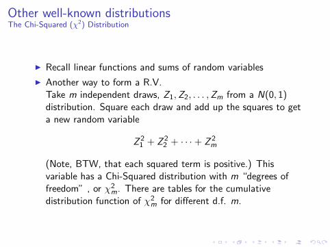
Other well-known distributionsThe Chi-Squared (χ2) Distribution

I Recall linear functions and sums of random variables

I Another way to form a R.V.Take m independent draws, Z1,Z2, . . . ,Zm from a N(0, 1)distribution. Square each draw and add up the squares to geta new random variable

Z 21 + Z 2

2 + · · · + Z 2m

(Note, BTW, that each squared term is positive.) Thisvariable has a Chi-Squared distribution with m “degrees offreedom” , or χ2

m. There are tables for the cumulativedistribution function of χ2

m for different d.f. m.

Other well-known distributionsThe Fm,∞ Distribution

I Another way to form a R.V.Divide a chi-square random variable by m (the number ofdraws that went into constructing the chi-square). Thisrandom vairable has a Fm,∞ distribution, and again tables areavailable.

Other well-known distributionsThe Student’s t Distribution

I Another way to form a R.V.Draw a standard normal variable, Z , and then independentlydraw a chi-square random variable, W , with m degrees offreedom.The ratio, Z√

W /mhas a Student t distribution with m degrees

of freedom.The Student t distribution was discovered by a brewerystatistician William Sealy Gossett who published anonymouslybecause the Guiness brewery didn’t want to release itsimportant trade secret.The Student t distribution looks almost normal and becomescloser and closer to the standard normal as m gets large. Wewill spend much less time on the t-distribution than do manystatistics courses because we will rely heavily on the normalapproximation.

Random sampling

1. Population

2. Simple random sampling

The randomness of sampling is very important

1. The sample must be, on average, like the population (ordifferent in a well-understood way).

2. Stratified random samples can be used to insurerepresentation of subgroups in the population (estimates mustbe adjusted for stratification).

3. Non-random samplesI Convenience samples (Landon defeats Roosevelt)I Nonresponse biasI Purposive sampling (e.g., for qualitative research)

The sample average

Sample n “draws” from the population so that (1) each member ofthe population equally likely to be drawn and (2) the distributionof Yi is the same for all i . This method makes the samplerepresentative of the population in important ways.

Y ≡1

n(Y1 + Y2 + · · · + Yn) =

1

n

n∑

i=1

Yi

Why is Y a random variable?

Because each of the Yi in the sample is a random variable andbecause the sample was randomly drawn from the population.A different sample of Y1,Y2, . . . ,Yn would have meant a differentsample mean.

Demonstration with wage data

Usually we have just one sample, but we’ll take the liberty ofpretending that we can take more than one sample of size n = 300from a population of 11,130 wage earners.

clear

use stock_watson/datasets/cps_ch3.dta

keep ahe98

set seed 12345

gen random_order = uniform()

sort random_order

* Cheat by looking at the mean for all 2,603 observations

summarize ahe98

* If we sampled the first 300 observations

ci ahe98 in 1/300

* If we sampled the second 300 observations

ci ahe98 in 301/600

* If we sampled the last 300 observations

ci ahe98 in 2304/2603

The Sampling Distribution of the Sample AverageThe Mean of Y

E (Y ) = E (1

n

n∑

i=1

Yi) =1

n

n∑

i=1

E (Yi ) =1

nnE (Y ) = µY

The Sampling Distribution of the Sample AverageThe Variance of Y

var(Y ) = var(1

n

n∑

i=1

Yi)

=1

n2

n∑

i=1

var(Yi ) +1

n2

n∑

i=1

n∑

j=1,j 6=i

cov(Yi ,Yj)

=1

n2

n∑

i=1

var(Yi )

=n

n2var(Yi )

=1

nvar(Yi)

=σ2

Y

n

The Sampling Distribution of the Sample AverageThe Standard Deviation of Y

var(Y ) =σ2

Y

n

sd(Y ) ≡ σY ≡√

var(Y ) =σY√

n

Do not confuse the standard deviation of Y with the standarddeviation of Y !

I The spread of the data Y will not change as the sample sizegrows.

I The standard deviation of Y will shrink as the sample sizegrows because we become more certain about the true valueof the mean as the sample size grows.

I Utterly amazing fact: the precision of Y depends entirely onthe absolute size of the sample n, not whether n is largerelative to the size of the population!

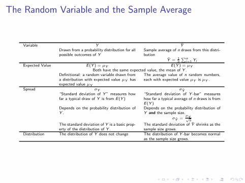
The Random Variable and the Sample Average

Variable Y Y

Drawn from a probability distribution for allpossible outcomes of Y

Sample average of n draws from this distri-bution

Y = 1n

Pni=1 Yi

Expected Value E(Y ) = µY E(Y ) = µYBoth have the same expected value, the mean of Y .

Definitional: a random variable drawn froma distribution with expected value µY hasexpected value µY

The average value of n random numbers,each with expected value µY is µY .

Spread σY σY“Standard deviation of Y ” measures howfar a typical draw of Y is from E(Y )

“Standard deviation of Y -bar” measureshow far a typical average of n draws is fromE(Y )

Depends on the probability distribution ofY .

Depends on the probability distribution ofY and the sample size.

σY =σY√

n

The standard deviation of Y is a basic prop-erty of the distribution of Y .

The standard deviation of Y shrinks as thesample size grows.

Distribution The distribution of Y does not change The distribution of Y -bar becomes normalas the sample size grows.

Large Sample Approximations

All we need is that Y1, . . . ,Yn be identically and independentlydistributed with E (Yi) = µY and var(Y ) = σ2

Y for two impressiveresults.

I Law of Large Numbers (LLN): When the sample size n islarge, the sample average Y is near the population mean µY

I Y “converges in probability” to µY

I Y “is consistent for” µY

I Central Limit Theorem (CLT): When the sample size n islarge, the sample average Y is normally distributed with meanµY and standard deviation σY (≡ σY /n). Or, equivalently,

Y − µY

σY

∼ N(0, 1)

This is true even if Y is not normally distributed.

Large Sample Approximations

Please be familiar with the meaning of the LLN and the CLT. Theproof of the LLN is fairly complicated. The proof of the CLT isvery complicated.These two results permit us to

1. use sample means to estimate population means; and

2. make inferences from sample means and variances.

Large Sample ApproximationsSome “experimental” evidence of the CLT

I Figures 2.6, 2.7, and 2.8.

I Is a Bernoulli variable normal? No, far from it because theoutcome is either 0 or 1. If n = 2, there are four possibleoutcomes: (0, 0), (0, 1), (1, 0), (1, 1), and the sample averagewill necessarily be 0, 1

2 , or 1, none of which is p = 0.78 in ourexample. However, as the sample size grows, the sampleaverage will frequently be near 0.78. For example, in a sampleof n = 1000, there might be 769 one’s and 231 zero’s, for asample average of 0.769. The LLN tells us that the sampleaverage will be near p = 0.78, and the CLT tells us that thedistribution around 0.78 will be normal.

I The same argument applies to another non-normal (in thiscase, highly skewed) distribution (Figure 2.8).

I n.b. To understand these diagrams, you must understand theidea of a sample, a sample mean, and a histogram of

sample means.

On to Statistics!