Distributionally Robust Performance Analysis: Data ...
121
Distributionally Robust Performance Analysis: Data, Dependence and Extremes Fei He Submitted in partial fulfillment of the requirements for the degree of Doctor of Philosophy in the Graduate School of Arts and Sciences COLUMBIA UNIVERSITY 2018
Transcript of Distributionally Robust Performance Analysis: Data ...
Distributionally RobustPerformance Analysis: Data,Dependence and Extremes
Fei He
Submitted in partial fulfillment of the
requirements for the degree
of Doctor of Philosophy
in the Graduate School of Arts and Sciences
COLUMBIA UNIVERSITY
2018

c©2018
Fei He
All Rights Reserved

ABSTRACT
Distributionally Robust Performance Analysis:Data, Dependence and Extremes
Fei He
This dissertation focuses on distributionally robust performance analysis, which is an
area of applied probability whose aim is to quantify the impact of model errors. Stochas-
tic models are built to describe phenomena of interest with the intent of gaining insights
or making informed decisions. Typically, however, the fidelity of these models (i.e. how
closely they describe the underlying reality) may be compromised due to either the lack
of information available or tractability considerations. The goal of distributionally robust
performance analysis is then to quantify, and potentially mitigate, the impact of errors
or model misspecifications. As such, distributionally robust performance analysis affects
virtually any area in which stochastic modelling is used for analysis or decision making.
This dissertation studies various aspects of distributionally robust performance analysis.
For example, we are concerned with quantifying the impact of model error in tail estimation
using extreme value theory. We are also concerned with the impact of the dependence
structure in risk analysis when marginal distributions of risk factors are known. In addition,
we also are interested in connections recently found to machine learning and other statistical
estimators which are based on distributionally robust optimization.
The first problem that we consider consists in studying the impact of model specifica-
tion in the context of extreme quantiles and tail probabilities. There is a rich statistical
theory that allows to extrapolate tail behavior based on limited information. This body
of theory is known as extreme value theory and it has been successfully applied to a wide
range of settings, including building physical infrastructure to withstand extreme environ-
mental events and also guiding the capital requirements of insurance companies to ensure
their financial solvency. Not surprisingly, attempting to extrapolate out into the tail of a

distribution from limited observations requires imposing assumptions which are impossible
to verify. The assumptions imposed in extreme value theory imply that a parametric family
of models (known as generalized extreme value distributions) can be used to perform tail
estimation. Because such assumptions are so difficult (or impossible) to be verified, we
use distributionally robust optimization to enhance extreme value statistical analysis. Our
approach results in a procedure which can be easily applied in conjunction with standard
extreme value analysis and we show that our estimators enjoy correct coverage even in
settings in which the assumptions imposed by extreme value theory fail to hold.
In addition to extreme value estimation, which is associated to risk analysis via extreme
events, another feature which often plays a role in the risk analysis is the impact of de-
pendence structure among risk factors. In the second chapter we study the question of
evaluating the worst-case expected cost involving two sources of uncertainty, each of them
with a specific marginal probability distribution. The worst-case expectation is optimized
over all joint probability distributions which are consistent with the marginal distributions
specified for each source of uncertainty. So, our formulation allows to capture the impact of
the dependence structure of the risk factors. This formulation is equivalent to the so-called
Monge-Kantorovich problem studied in optimal transport theory, whose theoretical prop-
erties have been studied in the literature substantially. However, rates of convergence of
computational algorithms for this problem have been studied only recently. We show that
if one of the random variables takes finitely many values, a direct Monte Carlo approach al-
lows to evaluate such worst case expectation with O(n−1/2) convergence rate as the number
of Monte Carlo samples, n, increases to infinity.
Next, we continue our investigation of worst-case expectations in the context of multiple
risk factors, not only two of them, assuming that their marginal probability distributions
are fixed. This problem does not fit the mold of standard optimal transport (or Monge-
Kantorovich) problems. We consider, however, cost functions which are separable in the
sense of being a sum of functions which depend on adjacent pairs of risk factors (think of
the factors indexed by time). In this setting, we are able to reduce the problem to the
study of several separate Monge-Kantorovich problems. Moreover, we explain how we can
even include martingale constraints which are often natural to consider in settings such as

financial applications.
While in the previous chapters we focused on the impact of tail modeling or dependence,
in the later parts of the dissertation we take a broader view by studying decisions which
are made based on empirical observations. So, we focus on so-called distributionally robust
optimization formulations. We use optimal transport theory to model the degree of distri-
butional uncertainty or model misspecification. Distributionally robust optimization based
on optimal transport has been a very active research topic in recent years, our contribution
consists in studying how to specify the optimal transport metric in a data-driven way. We
explain our procedure in the context of classification, which is of substantial importance in
machine learning applications.

Table of Contents
List of Figures iv
List of Tables v
1 Introduction 1
2 On Distributionally Robust Extreme Value Analysis 11
2.1 Introduction . . . . . . . . . . . . . . . . . . . . . . . . . . . . . . . . . . . . 11
2.1.1 Motivation and Standard Approach . . . . . . . . . . . . . . . . . . 12
2.1.2 Proposed Approach Based on Infinite Dimensional Optimization . . 13
2.1.3 Choosing Discrepancy and Consistency Results . . . . . . . . . . . . 14
2.1.4 The Final Estimation Procedure . . . . . . . . . . . . . . . . . . . . 16
2.2 Generalized extreme value distributions . . . . . . . . . . . . . . . . . . . . 16
2.2.1 Frechet, Gumbel and Weibull types . . . . . . . . . . . . . . . . . . . 17
2.2.2 On model errors and robustness . . . . . . . . . . . . . . . . . . . . 19
2.3 A non-parametric framework for addressing model errors . . . . . . . . . . . 20
2.3.1 Divergence measures . . . . . . . . . . . . . . . . . . . . . . . . . . . 20
2.3.2 Robust bounds via maximization of convex integral functionals . . . 21
2.4 Asymptotic analysis of robust estimates of tail probabilities . . . . . . . . . 24
2.5 Robust estimation of VaR . . . . . . . . . . . . . . . . . . . . . . . . . . . . 27
2.5.1 On specifying the parameter δ. . . . . . . . . . . . . . . . . . . . . . 30
2.5.2 On specifying the parameter α. . . . . . . . . . . . . . . . . . . . . . 31
2.5.3 Numerical examples . . . . . . . . . . . . . . . . . . . . . . . . . . . 34
i

2.6 Proofs of main results . . . . . . . . . . . . . . . . . . . . . . . . . . . . . . 39
3 Dependence with two sources of uncertainty: Computing Worst-case Ex-
pectations Given Marginals via Simulation 46
3.1 Algorithmic Description . . . . . . . . . . . . . . . . . . . . . . . . . . . . . 49
3.2 Convergence Analysis . . . . . . . . . . . . . . . . . . . . . . . . . . . . . . 49
3.2.1 Proof of Theorem 3.1 . . . . . . . . . . . . . . . . . . . . . . . . . . 50
3.3 Additional Discussion and Extensions . . . . . . . . . . . . . . . . . . . . . 55
4 Dependence with several sources of uncertainty: Martingale Optimal
Transport with the Markov Property 57
4.1 Introduction . . . . . . . . . . . . . . . . . . . . . . . . . . . . . . . . . . . . 57
4.2 Optimal Transport Problems with Two Marginal Distributions and Minimum
Cost Problems . . . . . . . . . . . . . . . . . . . . . . . . . . . . . . . . . . 59
4.2.1 Problem Definition . . . . . . . . . . . . . . . . . . . . . . . . . . . . 59
4.2.2 Quantization and Discretization . . . . . . . . . . . . . . . . . . . . 60
4.3 Optimal Transport Problems with d-Marginals . . . . . . . . . . . . . . . . 61
4.3.1 Discretization and Complexity . . . . . . . . . . . . . . . . . . . . . 62
4.4 Martingale Optimal Transport Problems with Separable Cost Functions and
the Markov Property . . . . . . . . . . . . . . . . . . . . . . . . . . . . . . . 63
4.4.1 Applications in Pricing Exotic Options . . . . . . . . . . . . . . . . . 66
4.5 A Numerical Experiment . . . . . . . . . . . . . . . . . . . . . . . . . . . . 68
5 Data-driven choice of the aspects over which to robustify: Data-driven
Optimal Transport Cost Selection and Doubly Robust Distributionally
Robust Optimization 70
5.1 Introduction . . . . . . . . . . . . . . . . . . . . . . . . . . . . . . . . . . . . 70
5.2 Data-Driven DRO: Intuition and Interpretations . . . . . . . . . . . . . . . 75
5.3 Background on Optimal Transport and Metric Learning Procedures . . . . 77
5.3.1 Defining Optimal Transport Distances and Discrepancies . . . . . . 77
5.3.2 On Metric Learning Procedures . . . . . . . . . . . . . . . . . . . . . 78
ii

5.4 Data Driven Cost Selection and Adaptive Regularization . . . . . . . . . . . 80
5.5 Solving Data Driven DRO Based on Optimal Transport Discrepancies . . . 82
5.6 Robust Metric Learning . . . . . . . . . . . . . . . . . . . . . . . . . . . . . 86
5.6.1 Robust Optimization for Relative Metric Learning . . . . . . . . . . 86
5.6.2 Robust Optimization for Absolute Metric Learning . . . . . . . . . . 88
5.7 Numerical Experiments . . . . . . . . . . . . . . . . . . . . . . . . . . . . . 91
5.7.1 Numerical Experiments for DD-DRO . . . . . . . . . . . . . . . . . . 91
5.7.2 Numerical Experiments for DD-R-DRO . . . . . . . . . . . . . . . . 92
5.8 Conclusion and Discussion . . . . . . . . . . . . . . . . . . . . . . . . . . . 93
5.9 Proof of Main Results . . . . . . . . . . . . . . . . . . . . . . . . . . . . . . 94
5.9.1 Proof of Theorem 5.1 . . . . . . . . . . . . . . . . . . . . . . . . . . 94
5.9.2 Proof of Lemma 5.1 . . . . . . . . . . . . . . . . . . . . . . . . . . . 97
Bibliography 98
iii
List of Figures
2.1 Comparison of Fα,δ(x) for different GEV models: The solid curves represents
the reference modelGγref(x) for γ
ref= 1/3 (top left figure), γ
ref= 0 (top right
figure) and γref
= −1/3 (bottom figure). Computations of corresponding
Fα,δ(x) are done for α = 1 (the dotted curves), and α = 5 (the dash-dot
curves) with δ fixed at 0.1. The dotted curves (corresponding to α = 1,
the KL-divergence case) conform with our reasoning that Fα,δ(x) have vastly
different tail behaviours from the reference models when KL-divergence is used. 29
2.2 Plots for Examples 2.2 and 2.3 . . . . . . . . . . . . . . . . . . . . . . . . . 35
2.3 Plot for Example 2.4, instability in estimated quantile F←(0.999) . . . . . . 37
5.1 Four diagrams illustrating information on robustness. . . . . . . . . . . . . . 75
5.2 Stylized examples illustrating the need for data-driven cost function. . . . 76
iv

List of Tables
2.1 A summary of domains of attraction of Fα,δ(x) = 1−Fα,δ(x) for GEV models.
Throughout the paper, γ∗ := αα−1γref
. . . . . . . . . . . . . . . . . . . . . . . . . . . . . . . . . . . . . . . . . . . 28
5.1 Numerical Results for DD-DRO on Real Data Sets. . . . . . . . . . . . . . . 92
5.2 Numerical Results for DD-R-DRO on Real Data Sets with Side Information
Generated by k-NN Method. . . . . . . . . . . . . . . . . . . . . . . . . . . 99
v

Acknowledgments
First and foremost, I would like to thank my advisor, Professor Jose Blanchet, for his
continued generous support. His broad knowledge, great insight and unwavering dedication
to research have always encouraged and inspired me to pursue interesting research topics
and helped me overcome many challenges and difficulties.
Besides my advisor, I would like to thank the rest of my committee members: Prof.
David Yao, Prof. Karl Sigman, Prof. Henry Lam and Prof. Jing Dong, for offering their
invaluable insight and expertise to improve my dissertation. I have learned much from
Prof. Yao and Prof. Sigman’s probability courses. Henry and Jing are also my research
collaborators and I really appreciate their guidance and patience during the collaboration.
I am also grateful to many IEOR professors, especially Prof. Garud Iyengar, Prof.
Martin Haugh, Prof. Agostino Capponi, Prof. Jay Sethuraman, Prof. Tim Leung and
Prof. Marcel Nutz, as well as many doctoral students and friends, especially Zhipeng Liu,
Yanan Pei, Anran Li, Yang Kang, Kartheyek Murthy, Ni Ma, Xinshang Wang, Mingxian
Zhong, Chaoxu Zhou, Francois Fagan, Octavio Ruiz Lacedelli, Di Xiao, Kevin Guo, Brian
Ward, Bin Qi, Yang Zhang, Yangbin Li, Xin Li, Zheng Wang, Jianshu Wu, Linan Yang,
Juan Li, Yin Lu, Yunhao Tang, Fan Zhang, Fengpei Li and Raghav Singal.
I would also like to thank Prof. Mark Podolskij, Prof. Rainer Dahlhaus, Prof. Tilmann
Gneiting, Yu Hao, Stefan Richter, Brandon Williams, Yuhong Dai, Nopporn Thamrongrat,
Cike Peng, Julie Yuan Merten, Shuxin Chen and Claudio Heinrich for their support and
help during my study in Germany. I am also much obliged to many friends in China:
Chengbin Peng, Hao Zhang, Junhui Zhang, Lu Chen, Huajie Mao, Hongyu Zhu, Wei Lin,
Minjie Zhang, Fang Lv, Hongyu Zhu, Bo Zhang, Wei Shi, Xiyuan Chen, Dingsheng Lin and
Yu Shi.
Last but not least, I am deeply indebted to my parents and Chris for their unconditional
vi

love and support over the years. No words can express my gratitude to them.
vii

Meinen Eltern und meinem Schatz
viii

CHAPTER 1. INTRODUCTION 1
Chapter 1
Introduction
This dissertation focuses on distributionally robust performance analysis, which is an area
of applied probability whose aim is to quantify the impact of model errors. Stochastic
models are built to describe phenomena of interest with the intent of gaining insights or
making informed decisions. Typically, however, the fidelity of these models (i.e. how closely
they describe the underlying reality) may be compromised by either the lack of information
available or by tractability considerations. The goal of distributionally robust performance
analysis is then to quantify, and potentially mitigate, the impact of errors or model mis-
specifications. As such, distributionally robust performance analysis affects virtually any
area in which stochastic modelling is used for analysis or decision making.
More specifically, in a stochastic model, the performance evaluation can be represented
as EP [h(X)] for a given probability measure P , a random variable X and a function h. A
modeler faces the task of choosing a probability model P which is not only close to the
reality but is also tractable. However, this procedure will often suffer from model errors,
either due to the lack of data or due to the estimation errors.
A popular approach to address this problem is by considering the distributionally robust
bound as the optimal value of the optimization problem
supP∈U
EP [h(X)],
over a family of plausible alternative probability models U . A natural way to specify the
family U is by defining an uncertainty neighborhood P : d(P, Pref ) ≤ δ, where Pref is the

CHAPTER 1. INTRODUCTION 2
chosen reference model and δ is a tolerance level. Here d is a metric which measures the
discrepancy between two probability measures. Popular choices for d are the KL-divergence
(Breuer and Csiszar (2013a), H.Lam (2013), Glasserman and Xu (2014a)) and the Wasser-
stein distances (Esfahani and Kuhn (2015), Wozabal (2012), Blanchet and Murthy (2016))
to quantify the model uncertainty. Despite the fact that KL-divergence is not a true metric,
KL-divergence is a popular choice due to its tractability. This approach provides a bound
for the performance evaluation regardless of the probability measure used as long as such
measures stay within a prescribed tolerance δ of an appropriate reference model.
In Chapter 2 we study the distributional robustness in the context of the extreme
value theory (EVT). Our focus is closer in spirit to distributionally robust optimizations
as in, for instance, Dupuis et al. (2000), Hansen and Sargent (2001), Ben-Tal et al. (2013),
Breuer and Csiszar (2013b). However, in contrast to the literature on robust optimization,
the emphasis here is on understanding the implications of distributional uncertainty regions
in the context of EVT. As far as we know this is the first paper that studies distributional
robustness in the context of EVT. Here, our objective is to provide a robust bound for the
estimate of the value at risk of a risk factor X,
VaRp(X) = F←(p) := infx : PX ≤ x ≥ p, for p ∈ (0, 1).
EVT provides reasonable statistical principles which can be used to extrapolate tail distri-
butions and then estimate this extreme quantiles. In particular, we focus on the classical
block maxima approach for the extrapolation, that is, we divide the i.i.d. data Xi into
several blocks, where each block contains n data points. Then we pick the maximum value
Mn from each block. The Fisher-Tippett-Gnedenko theorem ensures that under certain
assumptions of the underlying distribution of the Xi, the maximum Mn has some types
of limiting distribution PGEV , the so-called generalized extreme value distribution, and
produces P−1GEV (pn) as an estimate for the quantile VaRp(X). However, as with any form
for extrapolation, extreme value analysis rests on assumptions that are rather difficult (or
impossible) to verify. Therefore, it makes sense to provide a mechanism to robustify the
inference obtained via EVT. Similarly we formulate the robust estimate through an un-
certainty neighborhood of the limiting distribution with radius δ and then give a robust

CHAPTER 1. INTRODUCTION 3
estimate of VaRp(X) by
supG←(pn) : d(G,PGEV ) ≤ δ.
Here, we choose d as the Renyi divergence, also called the α-divergence, which includes
KL-divergence as a special case for α = 1. We show that using KL-divergence to form the
uncertainty set around PGEV would include a probability measure whose tail probabilities
decay at an unrealistically slow rate and the parameter α gives modeler the freedom to
tune the uncertainty set and include distributions with tails are heavier than the reference
model but not prohibitively heavy. We give concrete algorithms to calculate this robust
estimate and we also provide some practical ways to specify the hyperparameters α and the
radius of the uncertainty set δ. We also give some examples where the standard EVT can
significantly underestimate the quantiles of interest while our estimator is quite robust and
at the same time not too conservative.
In addition to extreme value estimation, which is associated to risk analysis via extreme
events, another feature which often plays a role in the risk analysis is the impact of de-
pendence structure among risk factors. Chapter 3 and Chapter 4 are devoted to find the
lower or upper bounds among any dependence structure with two sources of uncertainty or
multiple sources of uncertainty, that is, measuring the impact of the joint distribution with
two or multiple fixed marginals.
In Chapter 3 we study a direct Monte-Carlo-based approach for computing lower and
upper bounds among any dependence structure for a function of two random vectors whose
marginal distributions are assumed to be known.
More precisely, suppose that X ∈ Rd follows distribution µ and Y ∈ Rl follows dis-
tribution ν. We define Π (µ, ν) to be the set of joint distributions π in Rd×l such that
the marginal of the first d entries coincides with µ and the marginal of the last l entries
coincides with ν. In other words, for any probability measure π in Rd×l (endowed with the
Borel σ-field), if we let πX (A) = π(A× Rl
)for any Borel measurable set A ∈ Rd, and
πY (B) = π(Rd ×B
)for any Borel measurable set B ∈ Rl, then π ∈ Π (µ, ν) if and only if
πX = µ and πY = ν. We are interested in the quantity (focusing on minimization)
V = minEπ [c (X,Y )] : π ∈ Π (µ, ν) (1.1)

CHAPTER 1. INTRODUCTION 4
where c(·, ·) ∈ R is some cost function. Formulation (1.1) is well-defined as the class Π (µ, ν)
is non-empty, because the product measure π = µ × ν belongs to Π (µ, ν). The worst-case
expectation is optimized over all joint probability distributions which are consistent with the
marginal distributions specified for each source of uncertainty. So, our formulation allows
to capture the impact of the dependence structure of the risk factors. This formulation is
equivalent to the so-called Monge-Kantorovich problem studied in optimal transport theory,
whose theoretical properties have been studied in the literature substantially (Villani (2003),
Villani (2008)).
We focus on the setting where one of the marginals, say Y , has a distribution ν with
finite support y1, ..., ym ⊂ Rl and another, say X, has a multi-dimensional distribution µ
that can be continuous. Suppose we can i.i.d. sample Xi, i = 1, . . . , n from the distribution
µ then we approximate V by
Vn = minEπ [c (X,Y )] : π ∈ Π (µn, ν) (1.2)
where µn is the empirical distribution of X constructed from the Xi’s, i.e.,
µn(A) =1
n
n∑i=1
I(Xi ∈ A)
for any Borel measurable A.
Our main result shows that the error of our procedure is O(n−1/2) where n is the sample
size, independent of the dimension d or l. We also identify the limiting distribution in the
associated CLT. The closest work to our results, as far as we know, is the recent work of
Sommerfeld and Munk (2016), which derives a CLT when both marginal distributions are
finitely discrete.
On the other hand, it is difficult to further generalize our procedure to the case when
both X and Y are continuous. The study on the rate of convergence in Wasserstein distance
of the empirical measure gives ideas that in this general case the convergence rate fail to
retain O(n−1/2) (Fournier and Guillin (2015)). For instance, suppose both X,Y ∼ U [0, 1]d,
i.e. µ = ν are d-dim uniform distributions, and c(x, y) = ‖x − y‖, the optimal value V
corresponds to the Wasserstein distance (of order 1) between X and Y , which is of course
0. It is well-known that sampling X and keeping Y continuous will give, for d ≥ 3, an

CHAPTER 1. INTRODUCTION 5
expected optimal value of
Vn = minEπ [c (X,Y )] : π ∈ Π (µn, µ) µn(·) :=1
n
n∑i=1
I(Xi ∈ ·)
is of order n−1/d, i.e., C1n−1/d ≤ EVn ≤ C2n
−1/d for all n for some C1, C2 > 0 (see e.g.van
Handel (2014)).
In Chapter 4 we study a discretization approach for computing lower and upper
bounds among any dependence structure for a function of multiple random vectors whose
marginal distributions are assumed to be known. Given d marginal distributions µ1, . . . , µd
on a common compact metric space X , we focus on the lower bound
infπ∈Π(µ1,...,µd)
Eπ[c(X1, . . . , Xd)], (1.3)
where Π(µ1, . . . , µd) is the set of all joint distributions with marginals X1 ∼ µ1, . . . , Xd ∼ µd,
and c is a cost function. Note that when d = 2, the problem (1.3) is the standard optimal
transport problem. For d > 2, this problem has been studied by Gangbo and Swiech (1998)
and G.Carlier et al. (2008). Such problems often arise from risk management, where the
performance depends on d risk factors, and the marginal distributions of each risk factor is
known but the dependence structure is ambiguous.
We approach this problem by first create a partition of the compact space X with X =∑nk=1Ak such that the diameter of every Ak does not exceed δ, with δ = O(n−1). Then we
choose a representative xk ∈ Ak for each k and form a discrete set Xδ = xk : k = 1, . . . , n
with an associated quantization map
T : X →Xδ
x 7→n∑k=1
xkI(x ∈ Ak).
In addition, we define the corresponding quantized measures as
µ1,δ(xk) = µ1(Ak), · · · , µd,δ(xk) = µd(Ak), for k = 1, · · · , n (1.4)
CHAPTER 1. INTRODUCTION 6
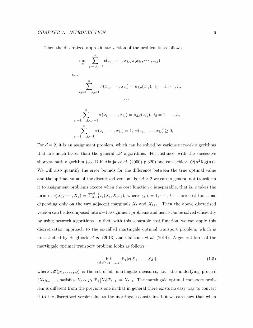
Then the discretized approximate version of the problem is as follows:
minπ
n∑i1,··· ,id=1
c(xi1 , · · · , xid)π(xi1 , · · · , xid)
s.t.
n∑i2=1,··· ,id=1
π(xi1 , · · · , xid) = µ1,δ(xi1), i1 = 1, · · · , n,
· · ·
n∑i1=1,··· ,id−1=1
π(xi1 , · · · , xid) = µd,δ(xid), id = 1, · · · , n,
n∑i1=1,··· ,id=1
π(xi1 , · · · , xid) = 1, π(xi1 , · · · , xid) ≥ 0,
For d = 2, it is an assignment problem, which can be solved by various network algorithms
that are much faster than the general LP algorithms. For instance, with the successive
shortest path algorithm (see R.K.Ahuja et al. (2000) p.320) one can achieve O(n2 log(n)).
We will also quantify the error bounds for the difference between the true optimal value
and the optimal value of the discretized version. For d > 2 we can in general not transform
it to assignment problems except when the cost function c is separable, that is, c takes the
form of c(X1, · · · , Xd) =∑d−1
k=1 ct(Xt, Xt+1), where ct, t = 1, · · · , d − 1 are cost functions
depending only on the two adjacent marginals Xt and Xt+1. Then the above discretized
version can be decomposed into d−1 assignment problems and hence can be solved efficiently
by using network algorithms. In fact, with this separable cost function, we can apply this
discretization approach to the so-called martingale optimal transport problem, which is
first studied by Beiglbock et al. (2013) and Galichon et al. (2014). A general form of the
martingale optimal transport problem looks as follows:
infπ∈M (µ1,...,µd)
Eπ[c(X1, . . . , Xd)], (1.5)
where M (µ1, . . . , µd) is the set of all martingale measures, i.e. the underlying process
(Xt)t=1,...,d satisfies Xt ∼ µt,Eπ[Xt|Ft−1] = Xt−1. The martingale optimal transport prob-
lem is different from the previous one in that in general there exists no easy way to convert
it to the discretized version due to the martingale constraint, but we can show that when
CHAPTER 1. INTRODUCTION 7
the cost function c is separable, then the problem can still be discretized to d − 1 linear
programming problems.
A major application of martingale optimal transport problem is in mathematical finance,
where it is important to choose a pricing model when evaluating an exotic option; such a
model is characterized by a martingale measure while the marginal distributions are the
daily underlying prices. Instead of postulating a model, we use (1.5) to give a model-free
lower bound for the price of exotics, whose payoff function c depends on the d-marginal
distributions of a certain underlying X, indexed by time t = 1, · · · , d. Similarly, by maxi-
mization instead of minimization we also obtain an upper bound for the price. This price
range is robust against model errors and it complies with market prices of vanilla options,
which are liquid and suitable hedging instruments. We provide some examples of financial
derivatives whose model-free price ranges can be obtained by our method.
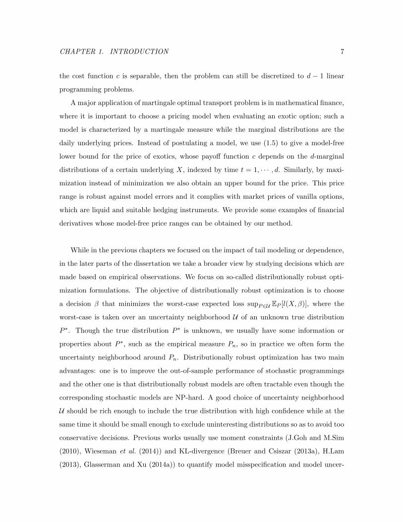
While in the previous chapters we focused on the impact of tail modeling or dependence,
in the later parts of the dissertation we take a broader view by studying decisions which are
made based on empirical observations. We focus on so-called distributionally robust opti-
mization formulations. The objective of distributionally robust optimization is to choose
a decision β that minimizes the worst-case expected loss supP∈U EP [l(X,β)], where the
worst-case is taken over an uncertainty neighborhood U of an unknown true distribution
P ∗. Though the true distribution P ∗ is unknown, we usually have some information or
properties about P ∗, such as the empirical measure Pn, so in practice we often form the
uncertainty neighborhood around Pn. Distributionally robust optimization has two main
advantages: one is to improve the out-of-sample performance of stochastic programmings
and the other one is that distributionally robust models are often tractable even though the
corresponding stochastic models are NP-hard. A good choice of uncertainty neighborhood
U should be rich enough to include the true distribution with high confidence while at the
same time it should be small enough to exclude uninteresting distributions so as to avoid too
conservative decisions. Previous works usually use moment constraints (J.Goh and M.Sim
(2010), Wieseman et al. (2014)) and KL-divergence (Breuer and Csiszar (2013a), H.Lam
(2013), Glasserman and Xu (2014a)) to quantify model misspecification and model uncer-

CHAPTER 1. INTRODUCTION 8
tainty. Despite the fact that KL-divergence is not a true metric, it is a popular choice due
to its tractability. However, many of these earlier works also acknowledge the shortcom-
ings of KL-divergence, as the absolute continuity requirement rules out many interesting
settings. For instance, all the probability measures in the neighborhood of an empirical
measure defined by the KL-divergence are just re-weighting of this empirical measure; the
neighborhood fails to include any continuous measures. Recently, people start applying
Wasserstein distance to distributionally robust optimization and quantify model misspeci-
fication (Wozabal (2012), Esfahani and Kuhn (2015), Blanchet and Murthy (2016)). When
the cost function c is a metric, i.e. c(x, y) = d(x, y), then the optimal transport problem
actually induces a metric called the Wasserstein distance or the optimal transport metric,
which characterizes a distance between the two probability measures µ and ν, and in turn
we can use it to define a neighborhood of a measure and apply it to the distributionally
robust problems. The uncertainty set contains both continuous and discrete distributions
that are close to the measure of interest (e.g. the empirical measure) with respect to the
Wasserstein distance, which makes it possible to incorporate many tractable surrogate mod-
els and offers better out-of-sample performance. However, distributionally robust models
with Wasserstein uncertainty neighborhood are generally harder in computations and they
are still attractive topics in research.
Chapter 5 uses optimal transport theory to model the degree of distributional uncer-
tainty or model misspecification, and extends the following distributionally robust optimiza-
tion (DRO) model proposed by Blanchet et al. (2016a), where they reveal that the DRO
models links to several machine learning algorithms such as regularized logistic regression
for classification,
minβ
maxP∈Uδ(Pn)
EP [l(X,Y, β)] = minβ
(EPn [l(X,Y, β)] + δ ‖β‖p
), (1.6)
where l is some loss function, and Uδ (Pn) = P : Dc(P, Pn) ≤ δ is a neighborhood of the
empirical measure Pn defined by the optimal transport distance
Dc (P, Pn) = infπ
Eπ[c(P, Pn)] : π is a joint distribution of P and Pn
and the optimal transport cost function
c((x, y), (x′, y′)) =∥∥x− x′∥∥2
qI(y = y′) +∞ · I(y 6= y′),

CHAPTER 1. INTRODUCTION 9
where p−1 + q−1 = 1 for p ∈ [1,∞), and EPn [l(X,Y, β)] := 1n
∑ni=1 l(Xi, Yi, β). We can
interpret the DRO problem on the left hand side of (1.6) as we choose a decision β for
minimization, while the adversarial player selects a model P , a perturbation of the data Pn,
from Uδ(Pn). This interpretation has applications in adversarial training of neural networks,
see e.g. Sinha et al. (2017). Note that the shape of Uδ(Pn) is determined by the cost function
c (·) in the definition of the optimal transport discrepancy Dc(P, Pn), but so far it has been
taken as a given `q-norm, but not chosen in a data-driven way; this is the starting point of
this project to improve the DRO method.
Our contribution consists in studying how to specify the optimal transport metric in a
data-driven way. We would propose a data-driven DRO (DD-DRO) model with the cost
function cΛ defined by a local metric dΛ(x, x′) :=√
(x− x′)TΛ(x)(x− x′), where the matrix
Λ(x) is trained by metric learning methods, see, e.g. Bellet et al. (2013). Note that when we
use a data-driven cost function, we may no longer have correspondence as (1.6) but we can
still directly solve the DRO problem on the left hand side. We expect that DD-DRO is able
to improve the generalization property compared to many other state-of-the-art classifiers
on a large number of data sets from UCI machine learning database, because it exploits the
side information (the information about the intrinsic metric, the “shape”) of the data.
The main methodologies and contributions of this project are the followings:
• We would use DRO as a link that combines k-NN methods with logistic regressions
for classification. We use k-NN method to generate the side information of the data
and then form the shape of the distributional uncertainty neighborhood by learning
a metric from this side information.
• The DD-DRO is able to recover adaptive regularized ridge regression estimator. The
DD-DRO provides a novel and interpretable way to select hyper-parameters in adap-
tive regularized ridge regression (see e.g.Zou (2006)) from a metric learning perspec-
tive.
• We would use an approximation algorithm based on stochastic gradient descent to
solve DD-DRO. We would reformulate the DRO problem by using the duality repre-
sentation given in Blanchet and Murthy (2016) and then solve it by smooth approxi-

CHAPTER 1. INTRODUCTION 10
mation and stochastic gradient descend algorithms.
• We would employ the robust metric learning to deal with the noisiness of side infor-
mation. Since the side information is usually noisy, we borrow the idea from robust
optimization (see e.g. Ben-Tal et al. (2009)) and build a doubly robust data-driven dis-
tributionally robust optimization (DD-R-DRO) model on top of the DD-DRO model
to achieve robust metric learning.

CHAPTER 2. ON DISTRIBUTIONALLY ROBUST EXTREME VALUE ANALYSIS 11
Chapter 2
On Distributionally Robust
Extreme Value Analysis
2.1 Introduction
Extreme Value Theory (EVT) provides reasonable statistical principles which can be used
to extrapolate tail distributions, and, consequently, estimate extreme quantiles. However,
as with any form for extrapolation, extreme value analysis rests on assumptions that are
rather difficult (or impossible) to verify. Therefore, it makes sense to provide a mechanism
to robustify the inference obtained via EVT.
The goal of this paper is to study non-parametric distributional robustness (i.e. find-
ing the worst case distribution within some discrepancy of a natural baseline model) in
the context of EVT. We ultimately provide a data-driven method for estimating extreme
quantiles in a manner that is robust against possibly incorrect model assumptions. Our
objective here is different from standard statistical robustness which is concerned with data
contamination only (not model error); see, for example, Tsai et al. (2010), for this type of
analysis in the setting of EVT.
Our focus in this paper is closer in spirit to distributionally robust optimization as in,
for instance, Dupuis et al. (2000), Hansen and Sargent (2001), Ben-Tal et al. (2013), Breuer
and Csiszar (2013b). However, in contrast to the literature on robust optimization, the
emphasis here is on understanding the implications of distributional uncertainty regions in

CHAPTER 2. ON DISTRIBUTIONALLY ROBUST EXTREME VALUE ANALYSIS 12
the context of EVT. As far as we know this is the first paper that studies distributional
robustness in the context of EVT.
We now describe the content of the paper, following the logic which motivates the use
of EVT.
2.1.1 Motivation and Standard Approach
In order to provide a more detailed description of the content of this paper, its motivations,
the specific contributions, and the methods involved, let us invoke a couple of typical ex-
amples which motivate the use of extreme value theory. As a first example, consider the
problem of forecasting the necessary strength that is required for a skyscraper in New York
City to withstand a wind speed that gets exceeded only about once in 1000 years, using
wind speed data that is observed only over the last 200 years. In another instance, given
the losses observed during the last few decades, a reinsurance firm may want to compute,
as required by Solvency II standard, a capital requirement that is needed to withstand all
but about one loss in 200 years.
These tasks, and many others in practice, present a common challenge of extrapolating
tail distributions over regions involving unobserved evidence from available observations.
There are many reasonable ways of doing these types of extrapolations. One might take
advantage of physical principles and additional information, if available, in the windspeed
setting; or use economic principles in the reinsurance setting. In the absence of any funda-
mental principles which inform tail extrapolation of a random variable X, one may opt to
use purely statistical considerations.
One such statistical approach entails the application of the popular extremal types
theorem (see Section 2.2) to model the distribution of block maxima of a modestly large
number of samples of X, by a generalized extreme value (GEV) distribution. Once we
have a satisfactory model for the distribution of Mn = maxX1, . . . , Xn, evaluation of
any desired quantile of X is straighforward because of the relationship that P (Mn ≤ x) =
(P (X ≤ x))n for any x ∈ R. Another common approach is to use samples that exceed
a certain threshold to model conditional distribution of X exceeding the threshold. The
standard texts in extreme value theory (see, for example, Leadbetter et al. (1983),de Haan

CHAPTER 2. ON DISTRIBUTIONALLY ROBUST EXTREME VALUE ANALYSIS 13
and Ferreira (2006),Resnick (2008)) provide a comprehensive account of such standard
statistical approaches.
Regardless of the technique used, various assumptions underlying an application of a
result similar to the extremal types theorem might be subject to model error. Consequently,
it has been widely accepted that tail risk measures, particularly for high confidence levels,
can only be estimated with considerable statistical as well as model uncertainty (see, for
example, Jorion (2006)). The following remark due to Coles (2001) holds significance in this
discussion: “Though the GEV model is supported by mathematical argument, its use in
extrapolation is based on unverifiable assumptions, and measures of uncertainty on return
levels should properly be regarded as lower bounds that could be much greater if uncertainty
due to model correctness were taken into account.”
Despite these difficulties, however, EVT is widely used (see, for example, de Haan and
Ferreira (2006)) and regarded as a reasonable way of extrapolation to estimate extreme
quantiles.
2.1.2 Proposed Approach Based on Infinite Dimensional Optimization
We share the point of view that EVT is a reasonable approach, so we propose a procedure
that builds on the use of EVT to provide upper bounds which attempts to address the
types of errors discussed in the remark above from Coles (2001). For large values of n,
under the assumptions of EVT, the distribution of Mn lies close to, and appears like,
a GEV distribution. Therefore, instead of considering only the GEV distribution as a
candidate model, we propose a non-parametric approach. In particular, we consider a
family of probability models, all of which lie in a “neighborhood” of a GEV model, and
compute a conservative worst-case estimate of Value at risk (VaR) over all of these candidate
models. For p ∈ [0, 1], the value at risk VaRp(X) is defined as
VaRp(X) = F←(p) := infx : PX ≤ x ≥ p.
Mathematically, given a reference model, Pref
, which we consider to be obtained using
EVT (using a procedure such as the one outlined in the previous subsection), we consider

CHAPTER 2. ON DISTRIBUTIONALLY ROBUST EXTREME VALUE ANALYSIS 14
the optimization problem
sup
PX > x : d(P, P
ref) ≤ δ
. (2.1)
Note that the previous problem proposes optimizing over all probability measures that are
within a tolerance level δ (in terms of a suitable discrepancy measure d) from the chosen
baseline reference model Pref.
There is a wealth of literature that pursues this line of thought (see Dupuis et al. (2000),
Hansen and Sargent (2001), Ahmadi-Javid (2012), Ben-Tal et al. (2013),Breuer and Csiszar
(2013b),Glasserman and Xu (2014b)), but, no study has been carried out in the context of
EVT. Moreover, while the solvability of problems as in (2.1) have understandably received
a great deal of attention, the qualitative differences that arise by using various choices of
discrepancy measures, d, has not been explored, and this is an important contribution of this
paper. For tractability reasons, the usual choice for discrepancy d in the literature has been
KL-divergence. In Section 2.3 we study the solution to infinite dimensional optimization
problems such as (2.1) for a large class of discrepancies that includes KL-divergence as a
special case, and discuss how such problems can be solved at no significant computational
cost.
2.1.3 Choosing Discrepancy and Consistency Results
One of our main contributions in this paper is to systematically demonstrate the qualitative
differences that arise by using different choices of discrepancy measures d in (2.1). Since
our interest in the paper is limited to robust tail modeling via EVT, this narrow scope, in
turn, lets us analyse the qualitative differences that may arise because of different choices
of d.
As mentioned earlier, the KL-divergence1 is the most popular choice for d. In Section
2.4 we show that for any divergence neighborhood P, defined using d = KL-divergence
around a baseline reference Pref
, there exists a probability measure P in P that has tails
as heavy as
P (x,∞) ≥ c log−2 Pref
(x,∞),
1KL-divergence, and all other relevant divergence measures, are defined in Section 2.3.1

CHAPTER 2. ON DISTRIBUTIONALLY ROBUST EXTREME VALUE ANALYSIS 15
for a suitable constant c, and all large enough x. This means, irrespective of how small δ is
(smaller δ corresponds to smaller neighborhood P), a KL-divergence neighborhood around
a commonly used distribution (such as exponential, (or) Weibull (or) Pareto) typically
contains tail distributions that have infinite mean or variance, and whose tail probabilities
decay at an unrealistically slow rate (even logarithmically slow, like log−2 x, in the case
of reference models that behave like a power-law or Pareto distribution). As a result,
computations such as worst-case expected short-fall2 may turn out to be infinite. Such
worst-case analyses are neither useful nor interesting.
For our purposes, we also consider a general family of divergence measures Dα that
includes KL-divergence as a special case (when α = 1). It turns out that for any α > 1,
the divergence neighborhoods defined as in P : Dα(P, Pref
) ≤ δ consists of tails that are
heavier than Pref
, but not prohibitively heavy. More importantly, we prove a “consistency”
result in the sense that if the baseline reference model belongs to the maximum domain
of attraction of a GEV distribution with shape parameter γref, then the corresponding
worst-case tail distribution,
Fα(x) := supP (x,∞) : Dα(P, Pref
) ≤ δ, (2.2)
belongs to the maximum domain of attraction of a GEV distribution with shape parameter
γ∗ = (1− α−1)−1γref
(if it exists).
Since our robustification approach is built resting on EVT principles, we see this consis-
tency result as desirable. If a modeler who is familiar with certain type of data expects the
EVT inference to result in an estimated shape parameter which is positive, then the robus-
tification procedure should preserve this qualitative property. An analysis of the maximum
domain of attraction of the distribution Fα(x), depending on α and γref, is presented in
Section 2.4, along with a summary of the results in Table 1.
Note that the smaller the value of α, the larger the absolute value of shape parameter γ∗,
and consecutively, heavier the corresponding worst-case tail is. This indicates a gradation
in the rate of decay of worst-case tail probabilities as parameter α decreases to 1, with
2Similar to VaR, expected shortfall (or) conditional value at risk (referred as CVaR) is another widely
recognized risk measure.

CHAPTER 2. ON DISTRIBUTIONALLY ROBUST EXTREME VALUE ANALYSIS 16
the case α = 1 (corresponding to KL-divergence) representing the extreme heavy-tailed
behaviour. This gradation, as we shall see, offers a great deal of flexibility in modeling by
letting us incorporate domain knowledge (or) expert opinions on the tail behaviour. If a
modeler is suspicious about the EVT inference he/she could opt to select α = 1, but, as we
have mentioned earlier, this selection may result in pessimistic estimates.
The relevance of these results shall become more evident as we introduce the required
terminology in the forthcoming sections. Meanwhile, Table 2.1 and Figure 2.1 offer illus-
trative comparisons of Fα(x) for various choices of α.
2.1.4 The Final Estimation Procedure
The framework outlined in the previous subsections yields a data driven procedure for
estimating VaR which is presented in Section 2.5. A summary of the overall procedure is
given in Algorithm 2. The procedure is applied to various data sets, resulting in different
reference models, and we emphasize the choice of different discrepancy measures via the
parameter α. The numerical studies expose the salient points discussed in the previous
subsections and rigorously studied via our theorems. For instance, Example 3 shows how
the use of the KL divergence might lead to rather pessimistic estimates. Moreover, Example
4 illustrates how the direct application of EVT can severely underestimate the quantile of
interest, while the procedure that we advocate provides correct coverage for the extreme
quantile of interest.
The very last section of the paper, Section 2.6, contains technical proofs of various
results invoked in the development.
2.2 Generalized extreme value distributions
The objective of this section is to mainly fix notation and review properties of generalized
extreme value (GEV) distributions that are relevant for introducing and proving our main
results in Section 2.4. For a thorough introduction to GEV distributions and their applica-
tions to modeling extreme quantiles, we refer the readers to the wealth of literature that is
available (see, for example, Leadbetter et al. (1983), Embrechts et al. (1997), de Haan and

CHAPTER 2. ON DISTRIBUTIONALLY ROBUST EXTREME VALUE ANALYSIS 17
Ferreira (2006), Resnick (2008) and references therein).
If we use Mn to denote the maxima of n independent copies of a random variable X
with cumulative distribution funtion F (·), then extremal types theorem identifies all non-
degenerate distributions G(·) that may occur in the limiting relationship,
limn→∞
P
Mn − bn
an≤ x
= lim
n→∞Fn (anx+ bn) = G(x), (2.3)
for every continuity point x of G(·), with an and bn representing suitable scaling constants.
All such distributions G(x) that occur in the right-hand side of (2.3) are called extreme
value distributions.
Extremal types theorem (Fisher and Tippet (1928), Gnedenko (1943)). The class of
extreme value distributions is Gγ(ax+ b) with a > 0, b, γ ∈ R, and
Gγ(x) := exp(− (1 + γx)−1/γ
), 1 + γx > 0. (2.4)
If γ = 0, the right-hand side is interpreted as exp(− exp(−x)).
The extremal types theorem asserts that any G(x) that occurs in the right-hand side of
(2.3) must be of the form Gγ(ax + b). As a convention, any probability distribution F (x)
that gives rise to the limiting distribution G(x) = Gγ(ax + b) in (2.3) is said to belong to
the maximum domain of attraction of Gγ(x). In short, it is written as F ∈ D(Gγ). The
parameters γ, a > 0 and b are, respectively, called the shape, scale and location parameters.
From the above we have
P (Mn ≤ x) = P(Mn − bn
an≤ x− bn
an
)≈ Gγ0
(x− bnan
)=: Gγ0(a0x+ b0),
where γ0, an, bn are estimated by a parameter estimation technique such as maximum
likelihood and a0 := 1/an, b0 := −bn/an. We will use PGEV to denote the distribution
Gγ0(a0x+ b0).
2.2.1 Frechet, Gumbel and Weibull types
Though the limiting distributions Gγ(ax+b) seem to constitute a simple parametric family,
they include a wide-range of tail behaviours in their maximum domains of attraction, as

CHAPTER 2. ON DISTRIBUTIONALLY ROBUST EXTREME VALUE ANALYSIS 18
discussed below: For a distribution F, let F (x) = 1 − F (x) denote the corresponding tail
probabilities, and x∗F
= supx : F (x) < 1 denote the right endpoint of its support.
1) The Frechet Case (γ > 0). A distribution F ∈ D(Gγ) for some γ > 0, if and only
if right endpoint x∗F
is unbounded, and its tail probabilities satisfy
F (x) =L(x)
x1/γ, x > 0 (2.5)
for a function L(·) slowly varying at ∞3. As a consequence, moments greater than or
equal to 1/γ do not exist. Any distribution F (x) that lies in D(Gγ) for some γ > 0
is also said to belong to the maximum domain of attraction of a Frechet distribution
with parameter 1/γ. The Pareto distribution 1− F (x) = x−α ∧ 1 is an example for a
distribution that belongs to D(G1/α).
2) The Weibull case (γ < 0). Unlike the Frechet case, a distribution F ∈ D(Gγ) for
some γ < 0, if and only if its right endpoint x∗F
is finite, and its tail probabilities
satisfy
F (x∗F− ε) = ε−1/γL
(1
ε
), ε > 0 (2.6)
for a function L(·) slowly varying at ∞. A distribution that belongs to D(Gγ) for
some γ < 0 is also said to belong to the maximum domain of attraction of Weibull
family. The uniform distribution on the interval [0, 1] is an example that belongs to
this class of extreme value distributions.
3) The Gumbel case (γ = 0). A distribution F ∈ D(G0) if and only if
limt↑x∗
F
F (t+ xf(t))
F (t)= exp(−x), x ∈ R (2.7)
for a suitable positive function f(·). In general, the members of G0 have exponen-
tially decaying tails, and consequently, all moments exist. Probability distributions
F (·) that give rise to limiting distributions G0(ax+ b) are also said to belong to the
Gumbel domain of attraction. Common examples that belong to the Gumbel domain
of attraction include exponential and normal distributions.
3A function L : R→ R is said to be slowly varying at infinity if limx→∞ L(tx)/L(x) = 1 for every t > 0.
Common examples of slowly varying function include log x, log log x, 1− exp(−x), constants, etc.

CHAPTER 2. ON DISTRIBUTIONALLY ROBUST EXTREME VALUE ANALYSIS 19
Given a distribution function F, Proposition 2.1 is useful to test to determine its domain of
attraction:
Proposition 2.1. Suppose F ′′(x) exists and F ′(x) is positive for all x in some left neigh-
borhood of x∗F. If
limx↑x∗
F
(1− FF ′
)′(x) = γ, (2.8)
then F belongs to the domain of attraction of Gγ .
The proof of Proposition 2.1 and further details on the classification of extreme value
distributions can be found in any standard text on extreme value theory (see, for example,
Leadbetter et al. (1983) or de Haan and Ferreira (2006)).
2.2.2 On model errors and robustness
After identifying a suitable GEV model PGEV for the distribution of block maxima Mn, it
is common to utilize the relationship PMn ≤ x = PX ≤ xn, to compute a desired
extreme quantile of X. It is useful to remember that PGEV (−∞, x] is only an approxi-
mation for PMn ≤ x, and the quality of the approximation is, in turn, dependent on
the unknown distribution function F (see Resnick (2008),de Haan and Ferreira (2006)).
Therefore, in practice, one does not know the block-size n for which the GEV model PGEV
well-approximates the distribution of Mn. Even if a good choice of n is known, one cannot
often employ it in practice, because larger n means smaller m, and consequentially, the
inferential errors could be large. Due to the arbitrariness in the estimation procedures and
the nature of applications (calculating wind speeds for building sky-scrapers, building dykes
for preventing floods, etc.), it is desirable to have, in addition, a data-driven procedure that
yields a conservative upper bound for xp that is robust against model errors. To accom-
plish this, one can form a collection of competing probability models P, all of which appear
plausible as the distribution of Mn, and compute the maximum of pn-th quantile over all
the plausible models in P. This is indeed the objective of the sections that follow.
CHAPTER 2. ON DISTRIBUTIONALLY ROBUST EXTREME VALUE ANALYSIS 20
2.3 A non-parametric framework for addressing model errors
Let (Ω,F) be a measurable space and M1(F) denote the set of probability measures on
(Ω,F). Let us assume that a reference probability model Pref∈ M1(F) is inferred by
suitable modelling and estimation procedures from historical data. Naturally, this model is
not the same as the distribution from which the data has been generated, and is expected
only to be close to the data generating distribution. In the context of Section 2.2, the
model Pref
corresponds to PGEV , and the data generating model corresponds to the true
distribution of Mn. With slight perturbations in data, we would, in turn, be working with
a slightly different reference model. Therefore, it has been of recent interest to consider a
family of probability models P, all of which are plausible, and perform computations over
all the models in that family. Following the rich literature of robust optimization, where it
is common to describe the set of plausible models using distance measures (see Ben-Tal et
al. (2013)), we consider the set of plausible models to be of the form
P =P ∈M1(F) : d
(P, P
ref
)≤ δ
for some distance functional d : M1(F) ×M1(F) → R+ ∪ +∞, and a suitable δ > 0.
Since d(Pref, P
ref) = 0 for any reasonable distance functional, P
reflies in P. Therefore, for
any random variable X, along with the conventional computation of EPref
[X], one aims to
provide “robust” bounds,
infP∈P
EP [X] ≤ EPref
[X] ≤ supP∈P
EP [X].
Here, we follow the notation that EP [X] =∫XdP for any P ∈ M1(F). Since the state-
space Ω is uncountable, evaluation of the above sup and inf-bounds, in general, are infinite-
dimensional problems. However, as it has been shown in the recent works Breuer and
Csiszar (2013b),Glasserman and Xu (2014b), it is indeed possible to evaluate these robust
bounds for carefully chosen distance functionals d.
2.3.1 Divergence measures
Consider two probability measures P and Q on (Ω,F) such that P is absolutely continu-
ous with respect to Q. The Radon-Nikodym derivative dP/dQ is then well-defined. The
CHAPTER 2. ON DISTRIBUTIONALLY ROBUST EXTREME VALUE ANALYSIS 21
Kullback-Liebler divergence (or KL-divergence) of P from Q is defined as
D1(P,Q) := EQ
[dP
dQlog
(dP
dQ
)]. (2.9)
This quantity, also referred to as relative entropy (or) information divergence, arises in
various contexts in probability theory. For our purposes, it will be useful to consider a
general class of divergence measures that includes KL-divergence as a special case. For any
α > 1, the Renyi divergence of degree α is defined as:
Dα(P,Q) :=1
α− 1logEQ
[(dP
dQ
)α]. (2.10)
It is easy to verify that for every α, Dα(P,Q) = 0, if and only if P = Q. Additionally,
the map α 7→ Dα is nondecreasing, and continuous from the left. Letting α → 1 in (2.10)
yields the formula for KL-divergence D1(P,Q). Thus KL-divergence is a special case of the
family of Renyi divergences, when the parameter α equals 1. If the probability measure P
is not absolutely continuous with respect to Q, then Dα(P,Q) is taken as ∞. Though none
of these divergence measures form a metric on the space of probability measures, they have
been used in a variety of scientific disciplines to discriminate between probability measures.
For more details on the divergences Dα, see Renyi (1961),Liese and Vajda (1987).
2.3.2 Robust bounds via maximization of convex integral functionals
Recall that Pref
is the reference probability measure obtained via standard estimation pro-
cedures. Since the model Pref
could be misspecified, we consider all models that are not far
from Pref
in the sense quantified by divergence Dα, for any fixed α ≥ 1. Given a random
variable X, we consider optimization problems of form
Vα(δ) := supEP [X] : Dα(P, P
ref) ≤ δ
. (2.11)
Though KL-divergence has been a popular choice in defining sets of plausible probability
measures as above, use of divergences Dα, α 6= 1 is not new altogether: see Atar et al.
(2015),Glasserman and Xu (2014b). Due to the Radon-Nikodym theorem, Vα(δ) can be
alternatively written as,
Vα(δ) = supEP
ref[LX] : EP
ref[φα(L)] ≤ δ, EP
ref[L] = 1, L ≥ 0
, (2.12)
CHAPTER 2. ON DISTRIBUTIONALLY ROBUST EXTREME VALUE ANALYSIS 22
where L = dP/dPref and
φα(x) =
xα if α > 1,
x log x if α = 1
and δ =
exp ((α− 1)δ) if α > 1,
δ if α = 1.
(2.13)
A standard approach for solving optimization problems of the above form is to write
the corresponding dual problem as below:
Vα(δ) ≤ infλ>0,µ
supL≥0
EPref
[LX − λ
(φα(L)− δ
)+ µ(L− 1)
].
The above dual problem can, in turn, be relaxed by taking the sup inside the expectation:
Vα(δ) ≤ infλ>0,µ
λδ − µ+ λEP
ref
[supL≥0
(X + µ)
λL− φα(L)
]. (2.14)
By first order condition the inner supremum is solved by
L∗α(c1, c2) :=
c1 exp(c2X), if α = 1,
(c1 + c2X)1/(α−1)+ , if α > 1,
(2.15)
for some suitable constants c1 ∈ R, c2 > 0 when α > 1; and c1 ∈ (0, 1) and c2 > 0 when
α = 1. Then the following theorem is intuitive:
Theorem 2.2. Fix any α ≥ 1. For L∗α(c1, c2) defined as in (2.15), if there exists constants
c1 and c2 such that
L∗α(c1, c2) ≥ 0, EPref
[L∗α(c1, c2)] = 1 and EPref
[φα (L∗α(c1, c2))] = δ,
then L∗α(c1, c2) solves the optimization problem (2.12). The corresponding optimal value is
Vα(δ) = EPref
[L∗α(c1, c2)X] . (2.16)
Proof. Under the specified assumptions, when we plug L∗α(c1, c2) into the right-hand-side of
inequality (2.14), it is simplified to EPref
[L∗α(c1, c2)X], so we have Vα(δ) ≤ EPref
[L∗α(c1, c2)X].
On the other hand, since L∗α(c1, c2) satisfies all the constraints in the problem (2.12), we
have Vα(δ) ≥ EPref
[L∗α(c1, c2)X].
CHAPTER 2. ON DISTRIBUTIONALLY ROBUST EXTREME VALUE ANALYSIS 23
Remark 2.1. Let us say one can determine constants c1 and c2 for given X,α and δ. Then,
as a consequence of Theorem 2.2, the optimization problem (2.11) involving uncountably
many measures can, in turn, be solved by simply simulating X from the original reference
measure Pref, and multiplying by corresponding L∗α(c1, c2) to compute the expectation as
in (2.16).
A general theory for optimizing convex integral functionals of form (2.12), that includes a
bigger class of general divergence measures, can be found in Breuer and Csiszar (2013b). If
the random variable X above is an indicator function, then computation of bounds Vα(δ)
turns out to be even simpler, as illustrated in the example below:
Example 2.1. Let Pref
be a probability measure on (R,B(R)). For a given δ > 0 and α ≥
1, let us say we are interested in evaluating the worst-case tail probabilities
Fα,δ(x) := supP (x,∞) : Dα(P, Pref
) ≤ δ.
Consider the canonical mapping Z(ω) = ω, ω ∈ R. Then
Fα,δ(x) = supEP
ref[L1(Z > x)] : EP
ref[φα(L)] ≤ δ, EP
ref[L] = 1, L ≥ 0
.
is an optimization problem of the form (2.11). Therefore, due to Theorem 2.2 and equation
(2.15), the optimal L∗ has the form
L∗α(c1, c2) :=
c1 exp(c21(Z > x)), if α = 1,
(c1 + c21(Z > x))1/(α−1)+ , if α > 1,
When we consider the two cases of Z > x and Z ≤ x, and combine the range information on
c1, c2 following equation (2.15), the above formulation of L∗α(c1, c2) can further be simplified
to θ1(x,∞) + θ1(−∞, x] for some constants θ > 1 and θ ∈ (0, 1). Substituting for L∗ =
θ1(x,∞) + θ1(−∞, x] in the constraints EPref
[φα(L∗)] = δ and EPref
[L∗] = 1, we obtain
the following conclusion: Given x > 0, if there exists a θx > 1 such that
Pref
(x,∞)φα(θx) + Pref
(−∞, x]φα
(1− θxPref (x,∞)
Pref
(−∞, x]
)= δ, (2.17)
then Fα,δ(x) = θxPref (x,∞).
CHAPTER 2. ON DISTRIBUTIONALLY ROBUST EXTREME VALUE ANALYSIS 24
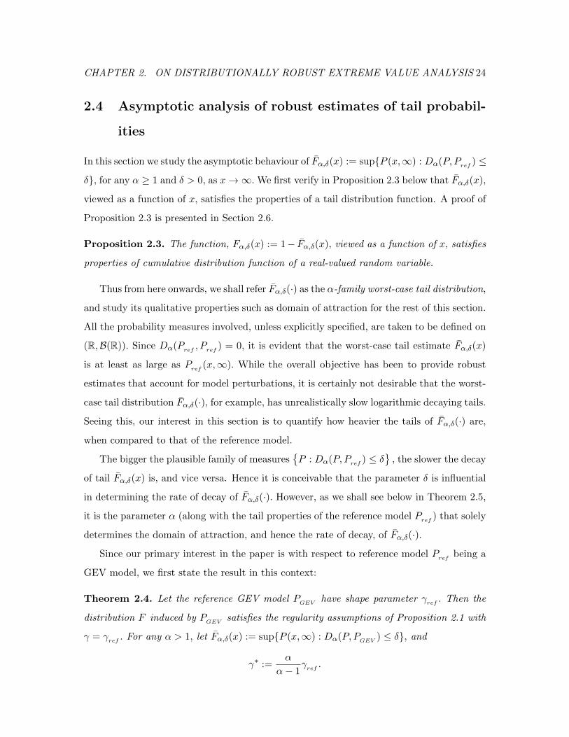
2.4 Asymptotic analysis of robust estimates of tail probabil-
ities
In this section we study the asymptotic behaviour of Fα,δ(x) := supP (x,∞) : Dα(P, Pref
) ≤
δ, for any α ≥ 1 and δ > 0, as x→∞. We first verify in Proposition 2.3 below that Fα,δ(x),
viewed as a function of x, satisfies the properties of a tail distribution function. A proof of
Proposition 2.3 is presented in Section 2.6.
Proposition 2.3. The function, Fα,δ(x) := 1− Fα,δ(x), viewed as a function of x, satisfies
properties of cumulative distribution function of a real-valued random variable.
Thus from here onwards, we shall refer Fα,δ(·) as the α-family worst-case tail distribution,
and study its qualitative properties such as domain of attraction for the rest of this section.
All the probability measures involved, unless explicitly specified, are taken to be defined on
(R,B(R)). Since Dα(Pref, P
ref) = 0, it is evident that the worst-case tail estimate Fα,δ(x)
is at least as large as Pref
(x,∞). While the overall objective has been to provide robust
estimates that account for model perturbations, it is certainly not desirable that the worst-
case tail distribution Fα,δ(·), for example, has unrealistically slow logarithmic decaying tails.
Seeing this, our interest in this section is to quantify how heavier the tails of Fα,δ(·) are,
when compared to that of the reference model.
The bigger the plausible family of measuresP : Dα(P, P
ref) ≤ δ
, the slower the decay
of tail Fα,δ(x) is, and vice versa. Hence it is conceivable that the parameter δ is influential
in determining the rate of decay of Fα,δ(·). However, as we shall see below in Theorem 2.5,
it is the parameter α (along with the tail properties of the reference model Pref
) that solely
determines the domain of attraction, and hence the rate of decay, of Fα,δ(·).
Since our primary interest in the paper is with respect to reference model Pref
being a
GEV model, we first state the result in this context:
Theorem 2.4. Let the reference GEV model PGEV have shape parameter γref. Then the
distribution F induced by PGEV satisfies the regularity assumptions of Proposition 2.1 with
γ = γref. For any α > 1, let Fα,δ(x) := supP (x,∞) : Dα(P, PGEV ) ≤ δ, and
γ∗ :=α
α− 1γref.

CHAPTER 2. ON DISTRIBUTIONALLY ROBUST EXTREME VALUE ANALYSIS 25
Then the distribution function Fα,δ(x) = 1− Fα,δ(x) belongs to the domain of attraction of
Gγ∗ .
Theorem 2.4 is, however, a corollary of Theorem 2.5 below.
Theorem 2.5. Let the reference model Pref
belong to the domain of attraction of Gγref.
In addition, let Pref
induce a distribution F that satisfies the regularity assumptions of
Proposition 2.1 with γ = γref. For any α > 1, let Fα,δ(x) := supP (x,∞) : Dα(P, P
ref) ≤
δ, and
γ∗ :=α
α− 1γref.
Then the distribution function Fα,δ(x) = 1 − Fα,δ(x) belongs to the maximum domain of
attraction of Gγ∗ .
The special case corresponding to α = 1 is handled in Propositions 2.6 and 2.7. Proofs
of Theorems 2.4 and 2.5 are presented in Section 2.6.
Remark 2.2. First, observe that P (x,∞) ≤ Fα,δ(x), for every P in the neighborhood
set of measures Pα,δ := P : Dα(P, Pref
) ≤ δ. Therefore, for any α > 1, apart from
characterizing the domain of attraction of Fα,δ, Theorem 2.5 offers the following insights on
the neighborhood Pα,δ :
1) If the reference model belongs to the domain of attraction of a Frechet distribution
(that is, γref
> 0), and if P is a probability measure that lies in its neighborhood
Pα,δ, then P must satisfy that
P (x,∞) = O
(x− α−1αγref
+ε), (2.18)
as x → ∞, for every ε > 0. This conclusion is a consequence of (2.5): Fα,δ is in the
domain of attraction of Gγ∗ , then by (2.5) we have
Fα,δ(x) = L(x)x−1/γ∗ = L(x)x− α−1αγref ,
and the observation that P (x,∞) ≤ Fα,δ(x). In addition, as in the proof of Theorem
2.5, one can exhibit a measure P ∈ Pα,δ such that P (x,∞) ≥ cx−(α−1)/αγref for some
c > 0 and all large enough x.

CHAPTER 2. ON DISTRIBUTIONALLY ROBUST EXTREME VALUE ANALYSIS 26
2) On the other hand, if the reference model belongs to the Gumbel domain of attraction
(γref
= 0), then every P ∈ Pα,δ satisfies P (x,∞) = o(x−ε), as x→∞, for every ε > 0.
3) Now consider the case where Pref∈ D(Gγref
) for some γref
< 0 (that is, the reference
model belongs to the domain of attraction of a Weibull distribution). Let x∗F< ∞
denote the supremum of its bounded support. In that case, any probability measure
P that belongs to the neighborhood Pα,δ must satisfy that P (−∞, x∗F
) = 1 and
P (x∗F− ε, x∗
F) = O
(ε− α−1αγref−ε′),
as ε→ 0, for every ε′ > 0. In addition, one can exhibit a measure P ∈ Pα,δ such that
P (x∗F− ε, x∗
F) ≥ cε−(α−1)/αγ
ref , for some positive constant c and all ε > 0 sufficiently
small.
It is important to remember that the above properties hold for all α > 1, and is not
dependent on δ.
For a fixed reference model Pref, it is evident from Remark 2.2 that the neighborhoods
Pα,δ = P : Dα(P, Pref
) ≤ δ include probability distributions with heavier and heavier
tails as α approaches 1 from above. This is in line with the observation that Dα(P, Pref
) is
a non-decreasing function in α, and hence larger neighborhoods Pα,δ for smaller values of α.
In particular, when α = 1 and shape parameter γref
= 0, the quantity γ∗ = γrefα/(α − 1)
defined in Theorem 2.4 is not well-defined. This corresponds to the set of plausible measures
P : D1(P,G0) ≤ δ defined using KL-divergence around the reference Gumbel model G0.
The following result describes the tail behaviour of Fα,δ in this case:
Proposition 2.6. Recall the definition of extreme value distributions Gγ in (2.4). Let
F1,δ(x) = supP (x,∞) : D1(P,G0) ≤ δ, and F1,δ(x) = 1 − F1,δ(x). Then F1,δ belongs to
the domain of attraction of G1.
The following result, when contrasted with Remark 2.2, better illustrates the difference
between the cases α > 1 and α = 1.
Proposition 2.7. Recall the definition of Gγ as in (2.4). For every δ > 0, one can find
a probability measure P in the neighborhood P : D1(P,Gγref) ≤ δ, along with positive
constants c+ or c− or c0, and x+ or x0 or ε− such that

CHAPTER 2. ON DISTRIBUTIONALLY ROBUST EXTREME VALUE ANALYSIS 27
a) P (x,∞) ≥ c+ log−3 x for every x > x+, if γref
> 0;
b) P (x,∞) ≥ c0x−1 for every x > x0, if γ
ref= 0; and
c) P (−∞, x∗G
) = 1 and P (x∗G− ε, x∗
G) ≥ c3 log−3 1
ε for every ε < ε−, if γref
< 0. Here,
the right endpoint x∗G
= supx : Gγref
(x) < 1 is finite because γref
< 0.
In addition, it is useful to contrast these tail decay results for neighboring measures with
that of the corresponding reference measure Gγrefcharacterized in (2.5), (2.6) or (2.7).
It is evident from this comparison that the worst-case tail probabilities Fα,δ(x) decay at
a significantly slower rate than the reference measure when α = 1 (the KL-divergence
case). Table 2.1 below summarizes the rates of decay of worst-case tail probabilities Fα,δ(·)
over different choices of α when the reference model is a GEV distribution. In addition,
Figure 2.1, which compares the worst-case tail distributions Fα,δ(x) for three different GEV
example models, is illustrative. Proofs of Theorems 2.4 and 2.5, Propositions 2.6 and 2.7
are presented in Section 2.6.
2.5 Robust estimation of VaR
Given independent samples X1, . . . , XN from an unknown distribution F, we consider the
problem of estimating F←(p) for values of p close to 1. In this section, we develop a
data-driven algorithm for estimating robust upper bounds for these extreme quantiles by
employing traditional extreme value theory in tandem with the insights derived in Sections
2.3 and 2.4. Our motivation has been to provide conservative estimates for F←(p) that are
robust against incorrect model assumptions as well as calibration errors.
Naturally, the first step in the estimation procedure is to arrive at a reference model
PGEV (−∞, x) = Gγ0(a0x + b0) for the distribution of block-maxima Mn. Once we have
a candidate model PGEV for Mn, the pn-th quantile of the distribution PGEV serves as an
estimator for F←(p). Instead, if we have a family of candidate models (as in Sections 2.3
and 2.4) for Mn, a corresponding robust alternative to this estimator is to compute the
worst-case quantile estimate over all the candidate models as below:
xp := supG←(pn) : Dα(G,PGEV ) ≤ δ
. (2.19)

CHAPTER 2. ON DISTRIBUTIONALLY ROBUST EXTREME VALUE ANALYSIS 28
Table 2.1: A summary of domains of attraction of Fα,δ(x) = 1 − Fα,δ(x) for GEV models.
Throughout the paper, γ∗ := αα−1γref
Domain of attraction of Domain of attraction of
Reference model Worst-case tail Fα,δ(·), α > 1 Worst-case tail Fα,δ(·), α = 1
(the KL-divergence case)
G0 G0 G1
(Gumbel light tails) (Gumbel light tails) (Frechet heavy tails)
Gγref, γ
ref> 0 Gγ∗ –
(Frechet heavy tails) (Frechet heavy tails) (slow logarithmic decay of
Fα,δ(x) as x→∞)
Gγref, γ
ref< 0 Gγ∗ –
(Weibull) (Weibull) (slow logarithmic decay of Fα,δ(x) to 0
at a finite right endpoint x∗)
Here G← denotes the usual inverse function G←(u) = infx : G(x) ≥ u with respect to
distribution G. Since the framework of Section 2.3 is limited to optimization over objective
functionals in the form of expectations (as in (2.11)), it is immediately not clear whether
the supremum in (2.19) can be evaluated using tools developed in Section 2.3. Therefore,
let us proceed with the following alternative: First, compute the worst-case tail distribution
Fα,δ(x) := sup G(x,∞) : Dα(G,PGEV ) ≤ δ , x ∈ R

CHAPTER 2. ON DISTRIBUTIONALLY ROBUST EXTREME VALUE ANALYSIS 29
Figure 2.1: Comparison of Fα,δ(x) for different GEV models: The solid curves represents
the reference model Gγref(x) for γ
ref= 1/3 (top left figure), γ
ref= 0 (top right figure) and
γref
= −1/3 (bottom figure). Computations of corresponding Fα,δ(x) are done for α = 1
(the dotted curves), and α = 5 (the dash-dot curves) with δ fixed at 0.1. The dotted curves
(corresponding to α = 1, the KL-divergence case) conform with our reasoning that Fα,δ(x)
have vastly different tail behaviours from the reference models when KL-divergence is used.
(a) G 13(x), a Frechet example (b) G0(x), a Gumbel example
(c) G− 13(x), a Weibull example
over all candidate models, and compute the corresponding inverse
F←α,δ(pn) := infx : 1− Fα,δ(x) ≥ pn.
The estimate xp (defined as in (2.19)) is indeed equal to F←α,δ(pn), and this is the content
of Lemma 2.1.
Lemma 2.1. For every u ∈ (0, 1), F←α,δ(u) = sup G←(u) : Dα(G,PGEV ) ≤ δ .
Proof. For brevity, let P = G : Dα(G,PGEV ) ≤ δ. Then, it follows from the definition of
CHAPTER 2. ON DISTRIBUTIONALLY ROBUST EXTREME VALUE ANALYSIS 30
Fα,δ(·) and F←α,δ(·) that
F←α,δ(u) = inf
x : sup
G∈PG(x,∞) ≤ 1− u
= inf
⋂G∈P
x : G(x,∞) ≤ 1− u
= inf
⋂G∈P
[G←(u),∞
)= sup
G∈PG←(u).
This completes the proof of Lemma 2.1.
Now that we know xp = F←α,δ(pn) is the desired upper bound, let us recall from Example
2.1 how to evaluate Fα,δ(x) for any x of interest. If θx > 1 solves
PGEV (x,∞)φα(θx) + PGEV (−∞, x)φα
(1− θxPGEV (x,∞)
PGEV (−∞, x)
)= δ,
then Fα,δ(x) = θxPGEV (x,∞). Though θx cannot be obtained in closed-form, given any
x > 0, one can numerically solve for θx, and compute Fα,δ(x) to a desired level of precision.
On the other hand, given a level u ∈ (0, 1), it is similarly possible to compute F←α,δ(u) by
solving for x that satisfies PGEV (x,∞) < 1− u and
PGEV (x,∞)φα
(1− u
PGEV (x,∞)
)+ PGEV (−∞, x)φα
(u
PGEV (−∞, x)
)= δ. (2.20)
Therefore, given α and δ, it is computationally not any more demanding to evaluate the
robust estimates F←α,δ(pn) for F←(p).
2.5.1 On specifying the parameter δ.
For a given choice of paramter α ≥ 1, there are several divergence estimation methods
available in the literature to obtain an estimate δ = Dα(PMn , PGEV ), where PMn is the
empirical distribution of Mn. For our examples, we use the k-nearest neighbor (k-NN)
algorithm of Poczos and Schneider (2011) and Q.Wang et al. (2009). See also Nguyen et al.
(2009),Nguyen et al. (2010),Gupta and Srivastava (2010) for similar divergence estimators.
These divergence estimation procedures provide an empirical estimate of the divergence
between sample maxima and the calibrated GEV model PGEV .
The specific details of the k-NN divergence estimation procedure we employ from Poczos
and Schneider (2011) and Q.Wang et al. (2009) are provided in Remark 2.3 below:

CHAPTER 2. ON DISTRIBUTIONALLY ROBUST EXTREME VALUE ANALYSIS 31
Remark 2.3. Suppose Mn,1, . . . ,Mn,m are independent samples of Mn, and L1, . . . , Ll are
samples from PGEV . Define ρk(i) to be the Euclidean distance between Mn,i and its k-th
nearest neighbour among all Mn,1, . . . ,Mn,m and similarly νk(i) the distance between Mn,i
and its k-th nearest neighbour among all L1, . . . , Ll. The k-NN based density estimators are
pk(Mn,i) =k/(m− 1)
|B(ρk(i))|and qk(Mn,i) =
k/l
|B(νk(i))|,
where |B(ρk(i))| denotes the volume of a ball with radius ρk(i). Then, for a fixed α, the
estimator for δ = Dα(PMn , PGEV ) is given by
δ =1
α− 1log
(1
m
m∑i=1
((m− 1)ρk(i)
lνk(i)
)1−α· Γ(k)2
Γ(k − α+ 1)Γ(k + α− 1)
),
for α > 1, where Γ denotes the gamma function, and
δ =1
m
m∑i=1
log( lνk(i)
(m− 1)ρk(i)
),
for α = 1.
For a fixed choice of α ≥ 1 and desired p close to 1, the Rob-Estimator(p, α) procedure
in Algorithm 1 below provides a summary of the prescribed estimation procedure.
2.5.2 On specifying the parameter α.
To input to the estimation procedure Rob-Estimator(p, α) in Algorithm 1, one can per-
haps choose α via one of the three approaches explained below:
1) Choose α so that the corresponding γ∗ = γ0α/(α − 1) matches with an appropriate
confidence interval for the estimate γ0 : For example, if γ0 > 0 and the confidence
interval for γ0, estimated from data, is given by (γ0 − ε, γ0 + ε), then we choose α
satisfying
γ0α
α− 1= γ0 + ε. (2.21)
See Examples 2.2 and 2.3 for demonstrations of choosing α following this approach.
2) Alternatively, one can choose α based on domain knowledge as well: For example,
consider the case where one uses Gaussian distribution to model returns of a portfolio.

CHAPTER 2. ON DISTRIBUTIONALLY ROBUST EXTREME VALUE ANALYSIS 32
In this instance, if a financial expert identifies the returns are instead heavy-tailed,
then one can take α = 1 to account for the imperfect assumption of Gaussian tails.
See Example 2.4 for a demonstration of choosing α based on this approach.
3) One can also adopt the following approach that mimicks the cross-validation proce-
Algorithm 1 To compute a robust upper bound xp for VaRp(X)
Given: N independent samples X1, . . . , XN of X, a level p close to 1, and a fixed choice
α ≥ 1.
procedure Rob-Estimator(p, α)
Initialize n < N, and let m = bNn c.
Step 1 (Compute block-maxima): Partition X1, . . . , XN into blocks of size n, and
compute the block maxima for each block to obtain samples Mn,1, . . . ,Mn,m of maxima
Mn.
Step 2 (Calibrate a reference GEV model): Treat the samples Mn,1, . . . ,Mn,m as
independent samples coming from a member of the GEV family and use a parameter
estimation technique (for example, maximum-likelihood) to estimate the parameters a0 , b0
and γ0 , along with suitable confidence intervals.
Step 3 (Determine the family of candidate models): For chosen α ≥ 1, determine δ
using a divergence estimation procedure (for an example, see Section 2.5.1). Then the
set P : Dα(P, PGEV ) ≤ δ represents the family of candidate models.
Step 4 (Compute the pn-th quantile for the reference GEV model, and as well as the
worst-case estimate over all candidate models):
Solve for x such that Gγ0(a0x+ b0) = pn, and let xp be the corresponding solution.
Solve for x > xp in (2.20) and let the solution be xp.
Return xp and xp

CHAPTER 2. ON DISTRIBUTIONALLY ROBUST EXTREME VALUE ANALYSIS 33
dure used in machine learning for choosing hyperparameters:
Recall that our objective is to estimate F←(p) for some p close to 1. With this ap-
proach, we first estimate F←(q) as a plug-in estimator from the empirical distribution,
for some q < p; while it is desirable that q is closer to p, care should be taken in the
choice that F←(q) should be estimable from the given N samples with high confi-
dence.
Having estimated F←(q) directly from the empirical distribution, the idea now is to
divide the given N samples, uniformly at random, into K mini-batches, each of which
is independently input as samples to the procedure Rob-Estimator(q, α) in Algo-
rithm 1 to yield K different robust estimates of F←(q) for an initially chosen value of
α (say, α = 1). If the mini-batches are of size N/r, then it is reasonable to choose the
scale-down factor r to be of the same order of magnitude as (1− q)/(1− p).
We repeat the above experiment for small increments of α to identify the largest value
of α for which the robust estimates obtained from the K sub-problems still cover the
plug-in estimate for F←(q) obtained initially from the empirical distribution. We uti-
lize this largest value of α that performs well in the scaled-down sub-problems to be
the choice of α for robust estimation of F←(p).
The third approach avoids using the upper end-point of a confidence interval of γ to
pick α. Instead it incorporates a trade-off between the choice of α and δ. Estimating
δ requires the estimation of the Renyi divergence, which is typically handled by k-NN
methods as explained in Remark 2.3. Large values of α may be desirable because they
generate better upper bounds, but since α → Dα is nondecreasing as mentioned in
Section 2.3.1, it also requires large neighborhoods to include the true distribution and
hence large values of δ. Further, by Theorem 2.5 if the true distribution has heavier
tail than the chosen GEV model, then there does exist a threshold of α over which the
neighborhoods will not include the true distribution or any other distributions with
the same or more tail heaviness than the true distribution, regardless of how large
δ is. Therefore when the chosen α is so large that the true distribution has the tail
with an index greater than γ∗, any attempt to estimate such δ will be unstable and
underestimated and causes the failure of coverage for true quantile. The above cross-

CHAPTER 2. ON DISTRIBUTIONALLY ROBUST EXTREME VALUE ANALYSIS 34
validation-like procedure incorporates this trade-off and picks a suitable pair (α, δ).
Example 2.5 gives the corresponding numerical experiments using this approach.
2.5.3 Numerical examples
Example 2.2. For a demonstration of the ideas introduced, we consider the rainfall accu-
mulation data, due to the study of Coles and Tawn (1996), from a location in south-west
England (see also Coles (2001) for further extreme value analysis with the dataset). Given
annual maxima of daily rainfall accumulations over a period of 48 years (1914-1962), we
attempt to compute, for example, the 100-year return level for the daily rainfall data. In
other words, we aim to estimate the daily rainfall accumulation level that is exceeded about
only once in 100 years. As a first step, we calibrate a GEV model for the annual maxima.
Maximum-likelihood estimation of parameters results in the following values for shape, scale
and location parameters: γ0 = 0.1072, a0 = 9.7284 and b0 = 40.7830. The 100-year return
level due to this model yields a point estimate 98.63mm with a standard error of ±17.67mm
(for 95% confidence interval). It is instructive to compare this with the corresponding es-
timate 106.3± 40.7mm obtained by fitting a generalized Pareto distribution (GPD) to the
large exceedances (see Example 4.4.1 of Coles (2001)). To illustrate our methodology, we
pick α = 2, as suggested in (2.21). Next, we obtain δ = 0.05 as an empirical estimate
of divergence Dα between the data points representing annual maxima and the calibrated
GEV model PGEV = Gγ0(a0x + b0). This step is accomplished using a simple k-nearest
neighbor estimator (see Poczos and Schneider (2011)). Consequently, the worst-case quan-
tile estimate over all probability measures satisfying Dα(P, PGEV ) ≤ δ is computed to be
F←α (1− 1/100) = 132.24mm. While not being overly conservative, this worst-case 100 year
return level of 132.44mm also acts as an upper bound to estimates obtained due to different
modelling assumptions (GEV vs GPD assumptions). To demonstrate the quality of esti-
mates throughout the tail, we plot the return levels for every 1/(1−p) years, for values of p
close to 1, in Figure 2.2(a). While the return levels predicted by the GEV reference model
is plotted in solid line (with the dash-dot lines representing 95% confidence intervals), the
dotted curve represents the worst-case estimates F←α (p). The empirical quantiles are drawn
in the dashed line.

CHAPTER 2. ON DISTRIBUTIONALLY ROBUST EXTREME VALUE ANALYSIS 35
Figure 2.2: Plots for Examples 2.2 and 2.3
(a) Quantile plots for rainfall data, Eg. 2.2
(b) Quantile plots for Pareto data, Eg. 2.3
Example 2.3. In this example, we are provided with 100 independent samples of a Pareto
random variable satisfying PX > x = 1− F (x) = 1 ∧ x−3. As before, the objective is to
compute quantiles F←(p) for values of p close to 1. As the entire probability distribution
is known beforehand, this offers an opportunity to compare the quantile estimates returned

CHAPTER 2. ON DISTRIBUTIONALLY ROBUST EXTREME VALUE ANALYSIS 36
by our algorithm with the actual quantiles. Unlike Example 2.2, the data in this example
does not present a natural means to choose block sizes. As a first choice, we choose block
size n = 5 and perform routine computations as in Algorithm 1 to obtain a reference
GEV model PGEV with parameters γ0 = 0.11, a0 = 0.58, b0 = 1.88, and corresponding
tolerance parameters α = 1.5 and δ = 0.8. Then the worst-case quantile estimate F←α (pn) =
supG←(pn) : Dα(G,PGEV ) ≤ δ is immediately calculated for various values of p close to 1,
and the result is plotted (in the dotted line) against the true quantiles F←(p) = (1− p)−1/3
(in the solid line) in Figure 2.2(b). These can, in turn, be compared with the quantile
estimates xp (in the solid line) due to traditional GEV extrapolation with reference model
PGEV . Recall that the initial choice for block size, n = 5, was arbitrary. One can perhaps
choose a different block size, which will result in a different model for corresponding block-
maximum Mn. For example, if we choose n = 10, the respective GEV model for M10 has
parameters γ0 = 0.22, a0 = 0.55 and b0 = 2.3. Whereas, if we choose n = 15, the GEV
model for M15 has parameters γ0 = 0.72, a0 = 0.32 and b0 = 2.66. When considering the
shape parameters, these models are different, and subsequently, the corresponding quantile
estimates (plotted using dashed lines in Figure 2.2(b)) are also different. However, as it can
be inferred from Figure 2.2(b), the robust quantile estimates (in the dotted line) obtained
by running Algorithm 1 forms a good upper bound to the actual quantiles F←(p), as well
as to the quantile estimates due to different GEV extrapolations from different block sizes
n = 10 and 15.
Example 2.4. The objective of this example is to demonstrate the applicability of Al-
gorithm 1 in an instance where the traditional extrapolation techniques tend to not yield
stable estimates. For this purpose, we use N = 2000 independent samples of the random
variable Y = X + 501(X > 5) as input to the maximum likelihood based GEV model
estimation, with the aim of calculating the extreme quantile F←(0.999). Here, F denotes
the distribution function of random variable Y, and X is a Pareto random variable with
distribution max(1 − x−1.1, 0). The quantile estimates (and the corresponding 95% confi-
dence intervals) output by this traditional GEV estimation procedure, for various choices of
block sizes, is displayed with the solid line in Figure 2.3. Even for modestly large block size
choices, it can be observed that the 95% confidence regions obtained from the calibrated
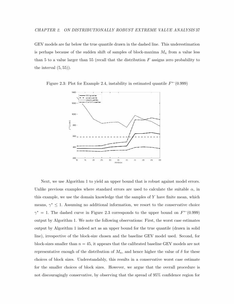
CHAPTER 2. ON DISTRIBUTIONALLY ROBUST EXTREME VALUE ANALYSIS 37
GEV models are far below the true quantile drawn in the dashed line. This underestimation
is perhaps because of the sudden shift of samples of block-maxima Mn from a value less
than 5 to a value larger than 55 (recall that the distribution F assigns zero probability to
the interval (5, 55)).
Figure 2.3: Plot for Example 2.4, instability in estimated quantile F←(0.999)
Next, we use Algorithm 1 to yield an upper bound that is robust against model errors.
Unlike previous examples where standard errors are used to calculate the suitable α, in
this example, we use the domain knowledge that the samples of Y have finite mean, which
means, γ∗ ≤ 1. Assuming no additional information, we resort to the conservative choice
γ∗ = 1. The dashed curve in Figure 2.3 corresponds to the upper bound on F←(0.999)
output by Algorithm 1. We note the following observations: First, the worst case estimates
output by Algorithm 1 indeed act as an upper bound for the true quantile (drawn in solid
line), irrespective of the block-size chosen and the baseline GEV model used. Second, for
block-sizes smaller than n = 45, it appears that the calibrated baseline GEV models are not
representative enough of the distribution of Mn, and hence higher the value of δ for these
choices of block sizes. Understandably, this results in a conservative worst case estimate
for the smaller choices of block sizes. However, we argue that the overall procedure is
not discouragingly conservative, by observing that the spread of 95% confidence region for

CHAPTER 2. ON DISTRIBUTIONALLY ROBUST EXTREME VALUE ANALYSIS 38
block size choices n = 50 to 60 (where the traditional GEV calibration appears correct) is
comparable to the difference between the true quantile and the worst-case estimate produced
by Algorithm 1 for majority of block size choices (from n = 20 to 60).
Example 2.5. In this example we consider the St. Petersburg distribution, which is not in
the maximum domain of attraction of any GEV distribution (see e.g. Fukker et al. (2016)).
Recall that X is St.Petersburg distributed if
PX = 2k = 2−k, k = 1, 2, . . . (2.22)
Note that the St. Petersburg distribution takes large values with tiny probability. Let B
denote a Bernoulli random variable with parameter 1/5. In addition let W be exponentially
distributed with mean 8 and define Z = B ·X +W. Suppose we have 5000 data points from
the distribution of Z. Similar to the previous example, we want to estimate its quantile
F←(0.999).
Here we demonstrate another approach to choose the parameter α. The idea, as described
earlier in Item 3) is to first choose a tail probability level q for which F←(q) can be accurately
estimated from the whole data set. For our example, we take q = 0.99 and compute the plug-
in estimate F←(q) from the empirical distribution. Then we independently divide the given
data set uniformly at random into 10 batches each of size 625 samples (corresponding to a
scale-down factor = 8). We employ the procedure Rob-Estimator(q, α) for various values
of α on each of these 10 sub-sampled mini-batches independently, and choose the largest
value of α such that the robust estimates from each of the 10 sub-samples cover the earlier
plug-in estimate F←(0.99). The specific details for this example are as follows:
1) The plug-in estimate for F←(0.99) from the given 5000 samples is 44.9. Note that with
5000 samples, this estimate from empirical distribution is with reasonably high confidence.
2) Resample the data into 10 mini-batches of size 5000/8 = 625 samples. With blocksize
= 20 we utilize the procedure Rob-Estimator(0.99, α) on each of the 10 mini-batches to
choose the largest α such that the respective robust estimates from all the 10 sub-sampled
mini-batches cover the empirical estimate of F←(0.99) obtained from step 1). This approach
leads us to the choice of α = 4.47. Computing block maxima from blocks of samples with size
= 48, the subsequent robust upper bound from the procedure Rob-Estimator(0.999, 4.47)

CHAPTER 2. ON DISTRIBUTIONALLY ROBUST EXTREME VALUE ANALYSIS 39
turns out to be 652.90, which covers the true quantile, F←(0.999) = 268.27. In contrast,
the 95%-confidence interval of GEV estimate is [93.81, 201.60], which fails to cover the true
quantile.
This approach incorporates the trade-off between the choice of α and δ. Large values of
α may be desirable because they generate less conservative upper bounds. But Step 2) avoids
picking too large values of α, because too large values of α, combined with the corresponding
estimators for δ empirically do not lead to good coverage for F←(0.99). Therefore this
cross-validation-like procedure automatically incorporates the trade-off between the choice of
hyperparameters α and δ.
2.6 Proofs of main results
In this section, we provide proofs of Theorems 2.4 and 2.5, along with proofs of Propositions
2.3, 2.6 and 2.7.
Proof of Proposition 2.3
By definition, Fα,δ(x) is non-decreasing in x. Since Fα,δ(x) ≤ Pref (−∞, x), we have limx→−∞ Fα,δ(x) =
0. In addition, we have from Example 2.1 that Fα,δ(x) = θxPref (x,∞), where θx satisfies
(2.17). Since Pref (x,∞)φα(θx) ≤ δ (follows from (2.17)), we have θx ≤ φ−1α (δ/Pref (x,∞)),
where φ−1α (·) is the inverse function of φα(·) (recall the defintion of φα(·) in (2.13) to see
that the inverse is well-defined for every α ≥ 1). As a result,
Fα,δ(x) ≤ φ−1α
(δ
Pref (x,∞)
)Pref (x,∞). (2.23)
If we let W (x) denote the product log function4, then φ−1α (u) = u−1/α when α > 1 and
φ−1α (u) = u/W (u) when α = 1. Consequently for any α ≥ 1, εφ−1
α (1/ε)→ 0 as ε→ 0. As a
result, limx→∞ Fα,δ(x) = 0 for any choice of α ≥ 1 and δ > 0. Thus limx→∞ Fα,δ(x) = 1.
4W is the inverse function of f(x) = xex

CHAPTER 2. ON DISTRIBUTIONALLY ROBUST EXTREME VALUE ANALYSIS 40
To show that Fα,δ(x) is right-continuous, we first see that
Fα,δ(x+ ε)− Fα,δ(x) = supP :Dα(P,Pref )≤δ
P (x,∞)− supP :Dα(P,Pref )≤δ
P (x+ ε,∞)
≤ supP :Dα(P,Pref )≤δ
P (x, x+ ε],
for any ε > 0, for every choice of δ > 0, α ≥ 1 and Pref . Following the same reasoning as in
(2.23), we obtain that
supP :Dα(P,Pref )≤δ
P (x, x+ ε] ≤ φ−1α
(δ
Pref (x, x+ ε]
)Pref (x, x+ ε],
for which the right hand side vanishes when ε→ 0. As a result, Fα,δ(x) is right-continuous
as well, thus verifying all the properties required to prove that Fα,δ(·) is a cumulative
distribution function.
Proof of Theorem 2.5
Our goal is to determine the maximum domain of attraction of Fα,δ(x) = supP (x,∞) :
Dα(P, Pref
) ≤ δ. We already have an upper bound for Fα,δ(x) in (2.23) in the proof of
Proposition 2.3. To obtain a lower bound for Fα,δ(x), first consider a probability measure
Q defined by
dQ
dPref
(x) = φ−1α
(c
Pref
(x,∞)(1− logPref
(x,∞))2
),
for a suitable positive constant c. Then Dα(Q,Pref
) < ∞ because of a simple change of
variables u = Pref
(x,∞) in the integration∫φα
(dQ
dPref
)dP
ref=
∫ 1
0
c
u(1− log u)2du <∞.
Consequently, due to a continuity argument, one can demonstrate a constant a ∈ (0, 1) such
that Dα(aQ+ (1− a)Pref, P
ref) ≤ δ. Then, it follows from the definition of Fα,δ(x) that
Fα,δ(x) ≥(aQ+ (1− a)P
ref
)(x,∞) =
∫ ∞x
(adQ
dPref
(t) + 1− a)Pref
(dt)
Since dQ/dPref
(t) is eventually increasing, as t→∞, we have that,
Fα,δ(x) ≥ aφ−1α
(c
Pref
(x,∞)(1− logPref
(x,∞))2
)Pref
(x,∞),
CHAPTER 2. ON DISTRIBUTIONALLY ROBUST EXTREME VALUE ANALYSIS 41
for sufficiently large values of x. For brevity, let
A(x) := Pref
(x,∞), g(x) := aφ−1α (c(1− log x)−2/x) and h(x) := φ−1
α (δ/x).
Then, combining the above lower bound with the upper bound in (2.23), we obtain
Flow(x) := g(A(x))A(x) ≤ Fα,δ(x) ≤ h(A(x))A(x) =: Fup(x), (2.24)
for large values of x. Recall that the reference measure Pref
belongs to the maximum domain
of attraction of Gγref. The following lemma characterizes the extreme value distributions
corresponding to the upper and lower bounds Fup and Flow.
Lemma 2.2. Suppose that the quantity γ∗ = αα−1γref is well-defined. Additionally, let
x∗ = supx : A(x) > 0. Then the following are true:
(a) limx↑x∗−
(FupF ′up
)′(x) = γ∗, and (b) lim
x↑x∗−(FlowF ′low
)′(x) = −γ∗.
As a consequence of Proposition 2.1 and Lemma 2.2, if γ∗ is finite, both Flow and Fup
lie in the maximum domain of attraction of Gγ∗ . As Fα,δ(x) is sandwiched between Flow(x)
and Fup(x) as in (2.24), if at all Fα,δ belongs to the maximum domain of attraction of Gγ
for some γ ∈ R, then γ must equal γ∗. Since Fα,δ(x) ∼ Fα,δ(x−) as x ↑ x∗, due to Theorem
1.7.13 of Leadbetter et al. (1983), this is indeed the case. Therefore, the α-family worst-case
tail distribution Fα,δ belongs to the maximum domain of attraction of Gγ∗ .
Proof of Lemma 2.2(a). Recall that Fup(x) = h(A(x))A(x). By repeatedly applying ele-
mentary rules of differentiation, it is obtained that
−
(FupF ′up
)′(x) = −
(A
A′
)′(x)
(1 +
A(x)h′(A(x))
h(A(x))
)−1
+
+
(A(x)h′(A(x))
h(A(x))+A2(x)
(h′
h
)′(A(x))
)(1 +
A(x)h′(A(x))
h(A(x))
)−2
(2.25)
Case α > 1 : Since h(x) = (δ/x)1/α and h′(x)/h(x) = −(αx)−1, we obtain
−
(FupF ′up
)′(x) = −
(A
A′
)′(x)
(1− 1
α
)−1
+
(− 1
α+
1
α
)(1− 1
α
)−2
.

CHAPTER 2. ON DISTRIBUTIONALLY ROBUST EXTREME VALUE ANALYSIS 42
In addition, as required in the statement of Theorem 2.5, A(x) := Pref
(x,∞) satisfies
−(A/A′)′(x)→ γref, as x approaches its right endpoint x∗ = supx : A(x) > 0. Therefore,
limx↑x∗−
(FupF ′up
)′(x) =
α
α− 1limx↑x∗
[−(A
A′
)′(x)
]=
α
α− 1γref.
Case α = 1 : When α equals 1, φ−1α (x) = x/W (x), where W (x) is the product log function.
Then the following calculations are simply algebraic:
xh′(x)
h(x)= −
1 +1
W(δx
)−1
and
x2
(h′
h
)′(x) =
[1 +
(1 +W
(δ
x
))−1]1 +
1
W(δx
)−2
.
Substituting these in (2.25), we obtain
−
(FupF ′up
)′(x) =
[−(A
A′
)′(x)W
(δ
A(x)
)− 1
]1 +1
W(
δA(x)
)−1
. (2.26)
Recall that −(A/A′)′(x) converges to γref, as x ↑ x∗. Letting x→ x∗ in the above expression,
we obtain
−
(FupF ′up
)′(x) =
∞, if γ
ref> 0,
−∞, if γref
< 0,
which indeed equals αα−1γref . This completes the proof of Part (a) of Lemma 2.2.
Proof of Lemma 2.2(b). First, an expression for (Flow/F′low)′ similar to (2.25) can be ob-
tained by simply substituting g in place of h in (2.25). Again, the cases α > 1 and α = 1
are calculated separately:
Case α > 1 : When α > 1, φ−1α (x) = x1/α. By applying elementary rules of differentiation,
we obtain
xg′(x)
g(x)=
1
α
1 + log x
1− log xand x2
(g′
g
)′(x) =
1
α
1 + log2 x
(1− log x)2.

CHAPTER 2. ON DISTRIBUTIONALLY ROBUST EXTREME VALUE ANALYSIS 43
Letting x ↑ x∗, we obtain A(x)g′(A(x))/g(A(x)) → −1/α and A(x)2(g′/g)′(A(x)) → 1/α.
Subsequently,
limx↑x∗
(FlowF ′low
)′(x) =
(1− 1
α
)−1
limx↑x∗
(A
A′
)′(x) +
(− 1
α+
1
α
)(1− 1
α
)2
,
which equals αα−1γref , as in the proof of Part (a) of Lemma 2.2. The case α = 1 is similar
to that of proof of Part (a), but more tedious, and is not presented here in the interest of
space and readability.
Proof of Theorem 2.4
Theorem 2.4 follows as a simple corollary of Theorem 2.5, once we verify that any GEV
model G(x) := PGEV (−∞, x) satisfies G′(x) > 0 and G′′(x) exists in a left neighborhood of
x∗G = supx : G(x) < 1, along with the property that
limx↑x∗G
(1−GG′
)′(x) = γ
ref,
where γref
is the shape parameter of G. Such a GEV model satisfies G(x) = Gγref(ax + b)
for some scaling and translation constants a and b. Therefore, it is enough to verify these
properties only for G(x) = Gγref(x). Once we recall the definition of Gγ in (2.4), the desired
properties are elementary exercises in calculus.
Proof of Proposition 2.6
First, we derive a lower bound for F1(x) = supP (x,∞) : D1(P,G0) ≤ δ. Consider the
probability density function f(x) = c(x log x)−21(x ≥ 2), where c is a normalizing constant
that makes∫f(x)dx = 1. In addition, let g(x) = G′0(x) denote the probability density
function corresponding to the distribution G0. Clearly,
D1(f, g) =
∫f(x) log
(f(x)
g(x)
)dx
= c
∫ ∞2
(x log x)−2 log
(c(x log x)−2
exp(− exp(−x) exp(−x))
)dx
≤∫ ∞
2
x+ exp(−x) + log c
x2 log2 xdx <∞.

CHAPTER 2. ON DISTRIBUTIONALLY ROBUST EXTREME VALUE ANALYSIS 44
Now, as in the proof of Theorem 2.5, consider a family of densities af + (1 − a)G′0 : a ∈
(0, 1). Due to the continuity of D1(af + (1 − a)G′0, G′0) with respect to a, there exists an
a ∈ (0, 1) such that D1(af + (1− a)G′0, G′0) ≤ δ. Then, according to the definition of F1,
F1(x) ≥∫ ∞x
(af + (1− a)G′0
)(u)du
≥ a∫ ∞x
c
u2 log2 udu =
ac+ o(1)
x log2 x,
as x → ∞. The asymptotic equivalence used above is due to Karamata’s theorem (see
Theorem 1 in Chapter VIII.9 of Feller (1966)). Combining this lower bound with the upper
bound in (2.23), we obtain, for large enough x,
ac
2x log2 x≤ F1(x) ≤ h
(1−G0(x)
)(1−G0(x)
),
where h(x) = φ−1α (δ/x). For convenience, let us write Fup(x) := h
(1−G0(x)
)(1−G0(x)
)and
Flow(x) := ac/(2x log2 x). Due to the characterization in (2.5), we have that Flow ∈ D(G1).
On the other hand, following the lines of Proof of Lemma 2.2(a), from (2.26), we obtain
that
−
(FupF ′up
)′(x) =
[(1−G0
G′0
)′(x)W
(δ
1−G0(x)
)+ 1
]1 +1
W(
δ1−G0(x)
)−1
.
Since G0(x) = exp(−e−x), we obtain(1−G0
G′0
)′(x) = ee
−x(ex(
1− e−e−x)− 1)
=e−x
2(1 + o(1)),
as x→∞. Therefore,
−
(FupF ′up
)′(x) ∼ e−x
2(1 + o(1))W
(δ
e−x(1 + o(1))
)+ 1
as x → ∞. Since tW (1/t) → 0 as t → 0, it follows that −(Fup/F′up)(x) converges to 1 as
x→∞. Then, due to Proposition 2.1, we have that Fup also belong to the maximum domain
of attraction of G1. Since both Flow and Fup lie in the maximum domain of attraction of
G1, following the same line of reasoning as in the proof of Theorem 2.5, we obtain that
F1(x) ∈ D(G1).

CHAPTER 2. ON DISTRIBUTIONALLY ROBUST EXTREME VALUE ANALYSIS 45
Proof of Proposition 2.7
First, let us consider the case γref6= 0: Recall the probability measure aQ + (1 − a)P
ref
exhibited for establishing the lower bound in the proof of Theorem 2.5. For proving
Proposition 2.7, we take the reference measure Pref
as Gγref. Further, if we let g(t) =
aφ−11 (c(1 − log t)−2/t) and A(x) := 1 − Gγref
(x), then as in the proof of Theorem 2.5, the
measure P := aQ+ (1− a)Pref
1) satisfies D1(P,Gγref) ≤ δ, and
2) admits a lower bound P (x,∞) ≥ g(A(x))A(x).
To proceed further, observe that A(x) = 1−Gγref(x) ≥ c(1+γ
refx)−1/γ
ref for some constant
c < 1 and all x close enough to the right endpoint x∗G
:= supx : Gγref(x) < 1. In addition,
tg(t) strictly decreases to 0 as t decreases to 0. Therefore, for all x close to the right endpoint
x∗G := supx : Gγref(x) < 1, it follows that
P (x,∞) ≥ g(c(1 + γ
refx)−1/γ
ref
)c(1 + γ
refx)−1/γ
ref .
Since φ−11 (u) ≥ u/ log u for large enough u, g(t) ≥ act−1 (1− log t)−2 log−1 (c/t), for all t
close to 0. As a result, there exists a constant c′ such that tg(t) ≥ c′(1 − log t)−3 for all t
sufficiently close to 0. This allows us to write
P (x,∞) ≥ c′(1− log(c(1 + γrefx)−1/γ
ref ))−3 = c′(1 + log(c1/γref (1 + γ
refx))/γ
ref)−3,
for x sufficiently close x∗G, thus verifying the statement in cases (a) and (b) where γ
ref6= 0.
When γref
= 0, see the proof of Proposition 2.6 where we exhibit a measure P such that
D1(P,G0) ≤ δ and P (x,∞) = O(x−1 log−2 x
). This completes the proof.

CHAPTER 3. DEPENDENCE WITH TWO SOURCES OF UNCERTAINTY:COMPUTING WORST-CASE EXPECTATIONS GIVEN MARGINALS VIASIMULATION 46
Chapter 3
Dependence with two sources of
uncertainty: Computing
Worst-case Expectations Given
Marginals via Simulation
We focus on the problem of computing lower and upper bounds among any dependence
structure for a function of two random vectors whose marginal distributions are assumed to
be known. This problem is motivated from several applications in risk quantification and
statistics. Before discussing its applications, let us first describe it precisely.
Suppose that X ∈ Rd follows distribution µ and Y ∈ Rl follows distribution ν. We
define Π (µ, ν) to be the set of joint distributions π in Rd×l such that the marginal of the
first d entries coincides with µ and the marginal of the last l entries coincides with ν. In
other words, for any probability measure π in Rd×l (endowed with the Borel σ-field), if we
let πX (A) = π(A× Rl
)for any Borel measurable set A ∈ Rd, and πY (B) = π
(Rd ×B
)for any Borel measurable set B ∈ Rl, then π ∈ Π (µ, ν) if and only if πX = µ and πY = ν.
We are interested in the quantity (focusing on minimization)
V = minEπ [c (X,Y )] : π ∈ Π (µ, ν) (3.1)
where c(·, ·) ∈ R is some cost function. Formulation (3.1) is well-defined as the class Π (µ, ν)

CHAPTER 3. DEPENDENCE WITH TWO SOURCES OF UNCERTAINTY:COMPUTING WORST-CASE EXPECTATIONS GIVEN MARGINALS VIASIMULATION 47
is non-empty, because the product measure π = µ× ν belongs to Π (µ, ν).
In operations research contexts, problem (3.1) arises as a means to obtain bounds for
performance measures in situations where dependence information is ambiguous. Such
situations occur because, in practice, accurately estimating the marginal distributions of
random variables is often relatively easy, e.g., by goodness-of-fit against well-chosen para-
metric distributions. They also occur in scenarios where data from different stochastic
sources are collected independently (i.e., rather than in pairs), in which case no dependence
information between these sources can be inferred. Indeed, special (i.e., discrete) cases
of (3.1) have been analyzed in the distributionally robust optimization literature (e.g.,
Doan et al. (2015)). Variants of (3.1) to risk measures have also been studied, regarding
both algorithmic approaches (e.g., Ruschendorf (1983), Embrechts et al. (2013)) and sharp
bounds over specific geometric classes of marginals (e.g., Wang and Wang (2011),Puccetti
(2013),Puccetti and Ruschendorf (2013)).
In statistics and machine learning contexts, the value of (3.1) is the Wasserstein dis-
tance (of order 1) between X and Y when c(·, ·) is taken as a metric. The optimization can
be viewed as the classical Kantorovich relaxation to Monge’s problem in optimal transport
(e.g., Rachev and Ruschendorf, Villani (1998, 2008)), where solutions based on differential
properties have been extensively studied. Wasserstein distance is of central importance in
probabilistic analysis (e.g., quantifying model discrepancies in Bayesian settings Minsker et
al. (2014) and convergence rates of ergodic processes Boissard and Le Gouic (2014), among
many others). The estimation of the distance itself is also suggested as a tool for statistical
inference, including the use in goodness-of-fit tests Del Barrio et al. (1999),Del Barrio et
al. (2005) and in applications such as image recognition Sommerfeld and Munk (2016). It
has also been used to quantify model uncertainty in stochastic optimization problems (e.g.,
Esfahani and Kuhn (2015),Blanchet and Kang (2016),Blanchet and Murthy (2016),Gao and
Kleywegt (2016)) and in the application of distributionally robust optimization in machine
learning settings Blanchet et al. (2016b). As such, there have been growing studies on the
convergence behaviors of its empirical estimation. Central limit theorems (CLTs) on the
empirical estimation of (3.1), based on representations using quantile functions, have been
investigated in the one-dimensional case (e.g., Bobkov and Ledoux (2014), Del Barrio et al.

CHAPTER 3. DEPENDENCE WITH TWO SOURCES OF UNCERTAINTY:COMPUTING WORST-CASE EXPECTATIONS GIVEN MARGINALS VIASIMULATION 48
(1999)). More generally, concentration bounds have been studied in the line of work includ-
ing Horowitz and Karandikar (1994), Bolley et al. (2007), Boissard (2011), Sriperumbudur
et al. (2012), Trillos and Slepcev (2014) and Fournier and Guillin (2015), so do laws of large
numbers in some special cases (e.g., Dobric and Yukich (1995)).
Since classical methods for solving (1), based for instance on Euler-Lagrange equations,
may not yield straightforward computational schemes in general, we resort to Monte Carlo
for an easy-to-implement approximation. Our contribution is precisely to quantify the rate
of convergence of such Monte Carlo schemes. Our results also add to the literature of
empirical Wasserstein estimation when these Monte Carlo samples are viewed as data. We
focus on the setting where one of the marginals, say Y , is a finite-support distribution, and
another, say X, is a multi-dimensional distribution that can be continuous. To approximate
V , we consider the drawn samples from the continuous variable X, and replace the infinite-
dimensional linear program (LP) in (3.1) by its sampled counterpart, which can be solved
by standard LP solvers.
Our main result shows that the error of our procedure is O(n−1/2) where n is the sample
size, independent of the dimension d or l. We also identify the limiting distribution in the
associated CLT. The closest work to our results, as far as we know, is the recent work of
Sommerfeld and Munk (2016), who derive a CLT when both marginal distributions are
finitely discrete. Our result here can be viewed as a generalization to theirs when one of
the distributions is continuous. We remark that our obtained rate differs from the typical
rate of O(n−1/d) in high-dimensional empirical Wasserstein estimation where d ≥ 3 is the
dimension of the marginal distributions. As we will see, the finite-support property of
one of the marginals plays a crucial role in applying classical results in sample average
approximation (SAA) that maintain the standard Monte Carlo rate in our scheme.
In the rest of this paper, we will first describe our algorithm, followed by our main
results on the convergence analysis.

CHAPTER 3. DEPENDENCE WITH TWO SOURCES OF UNCERTAINTY:COMPUTING WORST-CASE EXPECTATIONS GIVEN MARGINALS VIASIMULATION 49
3.1 Algorithmic Description
Suppose that the distribution ν for Y has finite support y1, ...ym ⊂ Rl. Supposing that
X can be simulated, we sample n i.i.d. observations X1, . . . , Xn from µ, and approximate
V by
Vn = minEπ [c (X,Y )] : π ∈ Π (µn, ν) (3.2)
where µn is the empirical distribution of X constructed from the Xi’s, i.e.,
µn(A) =1
n
n∑i=1
I(Xi ∈ A)
for any Borel measurable A.
Note that (3.2) is a finite-dimensional LP, which can be written more explicitly as
min∑n
i=1
∑mj=1 c(Xi, yj)pij
subject to∑m
j=1 pij = 1n ∀i = 1, . . . , n∑n
i=1 pij = νyj ∀j = 1, . . . ,m
pij ≥ 0 ∀i = 1, . . . , n, j = 1, . . . ,m
(3.3)
where the decision variables pij represent the probability masses on (Xi, yj), and νyj
denotes the mass on yj under ν. Problem (3.3) is an assignment problem, which is a
special type of minimum cost problem and can be solved by, e.g., successive shortest path
algorithms in polynomial time of order O(n2m+n(n+m) log(n+m)) (see, e.g., R.K.Ahuja
et al. (2000) pp. 471, 500).
3.2 Convergence Analysis
Our main result is a convergence analysis on Vn to V . We impose the assumptions:
Assumption 1. For each yj , c(., yj) is non-negative and lower semicontinuous.
Assumption 2. Suppose that ν has finite support y1, ..., ym ⊂ Rl. We have
Eµ[c(X, yj)2] <∞, ∀j = 1, . . . ,m.

CHAPTER 3. DEPENDENCE WITH TWO SOURCES OF UNCERTAINTY:COMPUTING WORST-CASE EXPECTATIONS GIVEN MARGINALS VIASIMULATION 50
Denote
V ′ = maxβ1,...,βm∈R
Eµ[
minj=1,...,m
c (X, yj)− βj+m∑j=1
βjνyj]
(3.4)
which is the dual problem of (3.1) (see Lemma 3.1 for an explanation in the special case
of finite-dimensional settings). Under Assumptions 1 and 2, strong duality (known as the
Kantorovich duality) holds and V ′ = V ; see, e.g., Theorem 5.10 in Villani (2008).
In order to state our main result, we need to introduce a Gaussian random field G(·) :
Rm → R with covariance structure given by
Cov(G(β), G(β′)) = Cov(
minj=1,...,m
c(X, yj)− βj
, minj=1,...,m
c(X, yj)− β′j
)for any β = (βj)
mj=1 and β′ = (β′j)
mj=1. Our main result is the following.
Theorem 3.1. Under Assumption 2, Vnp→ V ′ as n→∞. Moreover,
n1/2(Vn − V ′
)⇒ G∗
as n→∞, where
G∗ = maxβ=(β1,...,βm)∈S
G (β) .
Here S is the set of all optimal solutions β = (βj)mj=1 ∈ Rm for the convex optimization
problem
maxβ1,...,βm∈R∑mj=1 βj=0
Eµ[
minj=1,...,m
c (X, yj)− βj+m∑j=1
βjνyj]. (3.5)
Remark 3.1. The significance of this result is that one can approximate worst-case ex-
pectations by sampling with a rate of convergence (as measured by the sample size of the
continuous distribution) of order O(n−1/2). As we mentioned earlier, this might be some-
what surprising given that standard empirical estimators for Wasserstein distances exhibit
a degradation which becomes quite drastic in high dimensions.
3.2.1 Proof of Theorem 3.1
We first note that adding a constant to βj in the objective function of the dual does not
change the objective value. To remove this ambiguity we inroduce the next result.

CHAPTER 3. DEPENDENCE WITH TWO SOURCES OF UNCERTAINTY:COMPUTING WORST-CASE EXPECTATIONS GIVEN MARGINALS VIASIMULATION 51
Lemma 3.1. Define
Vn := maxβj∈R,j=1,...,m.∑m
j=1 βj=0
1
n
n∑i=1
minj=1,...,m
c(Xi, yj)− βj
+
m∑j=1
βjνyj
. (3.6)
We have Vn = Vn.
Proof. The dual formulation of Vn, depicted as the LP (3.3), is given by
max 1n
∑ni=1 αi +
∑mj=1 βjνyj
subject to αi + βj ≤ c(Xi, yj) ∀i = 1, . . . , n, j = 1, . . . ,m(3.7)
where (αi)mi=1, (βj)
mj=1 are the dual variables. Note that the constraint in (3.7) can be written
as αi ≤ minj=1,...,mc(Xi, yj)− βj ∀i = 1, . . . , n, which implies that (3.7) is equivalent to
maxβj∈R,j=1,...,m
1
n
n∑i=1
minj=1,...,m
c(Xi, yj)− βj
+
m∑j=1
βjνyj
(3.8)
Since shifting any (βj)mj=1 to (βj + λ)mj=1 by an arbitrary constant λ does not affect
the objective value of (3.8), we can always set λ = − 1m
∑mj=1 βj to enforce the constraint∑m
j=1 βj = 0, so that (3.8) is equal to (3.6). Finally, since (3.3) is feasible by choosing an
independent distribution, strong duality holds. We therefore conclude the lemma.
Next we show that Vn can be further reduced to a problem with compact feasible region,
which will subsequently facilitate the invocation of classical results in SAA:
Proposition 3.2. Define
V bn := max
βj∈R,|βj |≤b,j=1,...,m∑mj=1 βj=0
1
n
n∑i=1
minj=1,...,m
c(Xi, yj)− βj
+
m∑j=1
βjνyj
. (3.9)
There exists some large enough constant b > 0 such that
Vn = V bn (3.10)
eventually, i.e., holds for any n > N for some N <∞ almost surely.

CHAPTER 3. DEPENDENCE WITH TWO SOURCES OF UNCERTAINTY:COMPUTING WORST-CASE EXPECTATIONS GIVEN MARGINALS VIASIMULATION 52
Proof. By Lemma 3.1, we have
Vn = Vn
= max
max
βj∈R,|βj |≤b,j=1,...,m∑mj=1 βj=0
1
n
n∑i=1
minj=1,...,m
c(Xi, yj)− βj
+
m∑j=1
βjνyj
,
maxβj∈R,j=1,...,m,|βj |>b for some j∑m
j=1 βj=0
1
n
n∑i=1
minj=1,...,m
c(Xi, yj)− βj
+
m∑j=1
βjνyj
.(3.11)
Note that the first term inside the outer max is V bn by our definition (3.9). We will show
that there exists a deterministic b > 0 such that the first term dominates the second term
eventually, which will then conclude the proposition.
To this end, consider the second term in (3.11)
maxβj∈R,j=1,...,m,|βj |>b for some j∑m
j=1 βj=0
1
n
n∑i=1
minj=1,...,m
c(Xi, yj)− βj
+
m∑j=1
βjνyj
≤ maxβj∈R,j=1,...,m,|βj |>b for some j∑m
j=1 βj=0
min
j=1,...,m
− βj
+
m∑j=1
βjνyj
+1
n
n∑i=1
maxj=1,...,m
c(Xi, yj).
We analyze
maxβj∈R,j=1,...,m,|βj |>b for some j∑m
j=1 βj=0
min
j=1,...,m
− βj
+
m∑j=1
βjνyj. (3.12)
Denote M = maxj=1,...,m |βj |, so that M > b for any β inside the feasible region. There
must exist either a βj∗ = M or βj∗ = −M . In the first case, we have
maxβj∈R,j=1,...,m,|βj |>b for some j∑m
j=1 βj=0
min
j=1,...,m
− βj
+
m∑j=1
βjνyj
≤ −M +
max
∑mj=1 βjνyj
subject to βj ≤M ∀j = 1, . . . ,m∑mj=1 βj = 0
= −M +M ×
max
∑mj=1 βjνyj
subject to βj ≤ 1 ∀j = 1, . . . ,m∑mj=1 βj = 0
(3.13)

CHAPTER 3. DEPENDENCE WITH TWO SOURCES OF UNCERTAINTY:COMPUTING WORST-CASE EXPECTATIONS GIVEN MARGINALS VIASIMULATION 53
where the last equality follows by a change of variable from βj to βj/M in the optimization.
Note that the optimal value of
max∑m
j=1 βjνyj
subject to βj ≤ 1 ∀j = 1, . . . ,m∑mj=1 βj = 0
is strictly less than 1. To see this, observe that the optimal value is at most 1 by using
the first constraint. The value of exactly 1 is attained under the first constraint by the
unique solution βj = 1, j = 1, . . . ,m, which is ruled out because it would violate the second
constraint. With this claim, we conclude that (3.13) is equal to θM for some θ < 0, which
is bounded from above by θb.
In the second case, we have βj∗ = −M . Let j∗ = argmaxj=1,...,mβj. By the constraint∑mj=1 βj = 0 in (3.12), we must have βj∗ ≥M/(m− 1). Therefore, applying our argument
for the first case gives that (3.12) is bounded from above by θM/(m− 1) ≤ θb/(m− 1) for
the same θ < 0 chosen before.
Therefore, in either case (3.12) is bounded from above by θb/(m−1). Note that the first
term inside the outer max in (3.11), namely V bn , satisfies V b
n ≥ (1/n)∑n
i=1 minj=1,...,m c(Xi, yj)
by plugging in the feasible solution given by βj = 0, j = 1, . . . ,m. Thus, with the law of
large numbers, by choosing b > 0 large enough such that
θb
m− 1+ Eµ
[max
j=1,...,mc(X, yj)
]< Eµ
[min
j=1,...,mc(X, yj)
](3.14)
the first term dominates the second term inside the outer max in (3.11) as n → ∞ almost
surely.
We are now ready to prove Theorem 3.1:
Proof of Theorem 3.1. Note that the function
F (X,β) := minj=1,...,m
c(X, yj)− βj
+
m∑j=1
βjνyj (3.15)
on β = (βj)mj=1 ∈ Rm is Lipschitz continuous in the sense that
|F (X,β)− F (X,β′)| ≤ (1 + ‖ν‖)‖β − β′‖

CHAPTER 3. DEPENDENCE WITH TWO SOURCES OF UNCERTAINTY:COMPUTING WORST-CASE EXPECTATIONS GIVEN MARGINALS VIASIMULATION 54
where ‖ · ‖ denotes the L2-norm, and ν is interpreted as a vector (νyj)mj=1. This follows
since ∣∣∣∣ minj=1,...,m
c(X, yj)− βj
− minj=1,...,m
c(X, yj)− β′j
∣∣∣∣ ≤ ‖β − β′‖∞and ∣∣∣∣∣∣
m∑j=1
βjνyj −m∑j=1
β′jνyj
∣∣∣∣∣∣ ≤ ‖ν‖‖β − β′‖by the Cauchy-Schwarz inequality. Since the set B := β ∈ Rm :
∑mj=1 βj = 0, |βj | ≤ b,∀j =
1, . . . ,m is compact and Eµ[F (X,β)2] < ∞ by Assumption 2, by using Theorem 5.7 in
Shapiro et al. (2009), we have
V bn
p→ V b (3.16)
and√n(V b
n − V b)⇒ G∗,b (3.17)
where
V b = maxβj∈R,|βj |≤b,j=1,...,m∑m
j=1 βj=0
Eµ[
minj=1,...,m
c (X, yj)− βj+m∑j=1
βjνyj]
(3.18)
and
G∗,b = maxβ=(β1,...,βm)∈Sb
G (β)
with Sb denoting the set of optimal solutions for (3.18) and G(·) is defined as in Theorem
3.1 but restricted to the domain B.
By Proposition 3.2, we have√n(V b
n − Vn)p→ 0 as n → ∞. Thus, together with (3.16),
we have
Vnp→ V b
and together with (3.17), we have
√n(Vn − V b)⇒ G∗,b
by Slutsky’s Theorem.
To conclude the theorem, we show that V b = V ′, and Sb = S so that G∗,b = G∗. By
using essentially the same argument as for Proposition 3.2 (with the empirical expectation
CHAPTER 3. DEPENDENCE WITH TWO SOURCES OF UNCERTAINTY:COMPUTING WORST-CASE EXPECTATIONS GIVEN MARGINALS VIASIMULATION 55
replaced by Eµ[·]) and choosing the same b as in (3.14), we have
V ′ = maxβj∈R,j=1,...,m
Eµ[
minj=1,...,m
c (X, yj)− βj+
m∑j=1
βjνyj]
= maxβj∈R,j=1,...,m∑m
j=1 βj=0
Eµ[
minj=1,...,m
c (X, yj)− βj+m∑j=1
βjνyj]
by shifting any (βj)mj=1 to (βj − (1/m)
m∑k=1
βk)mj=1 which does not affect the objective value and
enforces the constraint
m∑j=1
βj = 0
= max
max
βj∈R,|βj |≤b,j=1,...,m∑mj=1 βj=0
Eµ[
minj=1,...,m
c (X, yj)− βj+
m∑j=1
βjνyj],
maxβj∈R,j=1,...,m,|βj |>b for some j∑m
j=1 βj=0
Eµ[
minj=1,...,m
c (X, yj)− βj+m∑j=1
βjνyj]
where
V b
= maxβj∈R,|βj |≤b,j=1,...,m∑m
j=1 βj=0
Eµ[
minj=1,...,m
c (X, yj)− βj+m∑j=1
βjνyj]
> maxβj∈R,j=1,...,m,|βj |>b for some j∑m
j=1 βj=0
Eµ[
minj=1,...,m
c (X, yj)− βj+m∑j=1
βjνyj]
so that V ′ = V b and Sb = S.
3.3 Additional Discussion and Extensions
Finally, we briefly discuss the challenge in generalizing our procedure to the case when both
X and Y are continuous. Here, one may attempt to sample both variables (assuming both
can be simulated) and formulate a sampled program like (3.2) or (3.3). However, the analog
of its reformulation in (3.6) and (3.9) will have a growing number of variables βj and an
analogous limit in (3.5) that involves an infinite-dimensional variable, which challenges the
use of standard SAA machinery. In fact, consider a special example where X,Y ∼ U [0, 1]d
CHAPTER 3. DEPENDENCE WITH TWO SOURCES OF UNCERTAINTY:COMPUTING WORST-CASE EXPECTATIONS GIVEN MARGINALS VIASIMULATION 56
and c(x, y) = ‖x− y‖. In this case, (3.1) corresponds to the Wasserstein distance (of order
1) between X and Y , which is of course 0. It is known that sampling X and keeping Y
continuous will give, for d ≥ 3, an expected optimal value of (3.2) that is of order n−1/d, i.e.,
C1n−1/d ≤ EVn ≤ C2n
−1/d for all n for some C1, C2 > 0 (e.g., Problem 5.11 in van Handel
(2014)). Thus, the convergence rate deteriorates with the dimension and the standard
Monte Carlo rate O(n−1/2) cannot be maintained without assuming additional structure or
infomation available to the modeler on the primal problem. It is of interest to investigate
reasonable assumptions which are useful in applications and which would mitigate such
rate-of-convergence deterioration.
CHAPTER 4. DEPENDENCE WITH SEVERAL SOURCES OF UNCERTAINTY:MARTINGALE OPTIMAL TRANSPORT WITH THE MARKOV PROPERTY 57
Chapter 4
Dependence with several sources of
uncertainty: Martingale Optimal
Transport with the Markov
Property
4.1 Introduction
In this chapter we study a discretization approach for computing lower and upper bounds
among any dependence structure for a function of multiple random variables whose marginal
distributions are assumed to be known. More specifically, given d ≥ 2 marginal distributions
µ1, . . . , µd on a common compact metric space X , we focus on the lower bound
infπ∈Π(µ1,...,µd)
Eπ[c(X1, . . . , Xd)], (4.1)
where Π(µ1, . . . , µd) is the set of all joint distributions with marginals X1 ∼ µ1, . . . , Xd ∼ µd,
and c is a cost function. For instance, in risk management, such situations often occur
when the estimation of marginal distributions of each risk factor Xi is relatively easy, but
the dependence structure among them is ambiguous. Given loss level ` > 0 and the cost
function c(X1, . . . , Xd) = I(X1 + · · ·+Xd > `) with d risk factors X1, . . . , Xd, the quantity

CHAPTER 4. DEPENDENCE WITH SEVERAL SOURCES OF UNCERTAINTY:MARTINGALE OPTIMAL TRANSPORT WITH THE MARKOV PROPERTY 58
infπ∈Π(µ1,...,µd) Eπ[c(X1, . . . , Xd)] gives a lower bound for the probability of the event that
the sum of these risk factors exceed the level `.
Note that when d = 2, the problem (4.1) is the standard optimal transport (or Monge-
Kantorovich) problem, whose theoretical properties have been studied in the literature
substantially(Villani (2003), Villani (2008)). For d > 2, this problem has been studied by
Gangbo and Swiech (1998) and G.Carlier et al. (2008).
Based on the above optimal transport problem (4.1), Beiglbock et al. (2013) and Gali-
chon et al. (2014) further develop the so-called martingale optimal transport problem, which
adds the martingale constraint to the joint distribution. The martingale optimal transport
problem has the following form
infπ∈M (µ1,...,µd)
Eπ[c(X1, . . . , Xd)],
where M (µ1, . . . , µd) is the set of all martingale measures, i.e. the underlying process
(Xt)t=1,...,d satisfies Xt ∼ µt,Eπ[Xt+1|Ft] = Xt for t = 1, . . . , d− 1.
In contrast to optimal transport problem where the product measure is always a feasible
solution, here the existence of martingale measure π requires some constraint on marginals:
for the feasibility of
P : X1 ∼ µ1, . . . , Xd ∼ µd;Eπ[Xt+1|Ft] = Xt for t = 1, . . . , d− 1,
we need the condition that all the marginals satisfy the convex order: µt ≤ µt+1, for
t = 1, . . . , d− 1 where µt ≤ µt+1 is defined as Eµt [ψ(Xt)] ≤ Eµt+1 [ψ(Xt+1)],∀ψ convex. See
H.G.Kellerer (1972).
The main motivation of studying martingale optimal transport problem stems from
the requirement of financial robustness against model risks. In finance, it is important to
choose a pricing model when evaluating an exotic option; such a model is characterized
by a martingale measure while the marginal distributions are the daily underlying prices.
Instead of postulating a model, (4.6) gives a model-free lower bound for the price of exotics,
whose payoff function c depends on the d-marginal distributions of a certain underlying X,
indexed by time t = 1, . . . , d. Similarly, by using maximization instead of minimization we

CHAPTER 4. DEPENDENCE WITH SEVERAL SOURCES OF UNCERTAINTY:MARTINGALE OPTIMAL TRANSPORT WITH THE MARKOV PROPERTY 59
also obtain an upper bound. This price range is robust against model errors and it complies
with market prices of vanilla options, which are liquid and suitable hedging instruments.
Previous literatures tackle the martingale optimal transport problems by numerically
solving the Hamilton-Jacobi-Bellman PDEs (Henry-Labordere and Touzi (2013)), but the
computational complexity is hard to track.
Compared to their numerical PDE approach, our discretization approach can obtain an
approximate solution within certain error under a much mild assumptions, both on the cost
function c and on the marginal distributions. We give the computational complexity for the
general optimal transport problem in high dimensions. And we also give a discretization
method for the martingale transport problem with a special type of cost functions and
provide a practical way of robustly pricing certain financial derivatives.
4.2 Optimal Transport Problems with Two Marginal Distri-
butions and Minimum Cost Problems
4.2.1 Problem Definition
For simplicity and to describe the idea of discretization, in this section we consider the
case of two given marginals. Let X be a compact metric space and P(X ) be the set of
probability measures on X . In this section, we only consider two (marginal) probability
measures. For µ, ν ∈P(X ), let Π(µ, ν) be the set of all joint probability measures with µ
and ν as marginals. We are interested in the following optimal transport problem
P := minπ∈Π(µ,ν)
∫c(x, y)dπ(x, y)
= min
π∈Π(µ,ν)Eπc(X,Y ) (4.2)
where the cost function c(·, ·) : X ×X → R is Lipschitz continuous with Lipschitz constant
K, and ‖c‖ ≤ 1.
In the following we will try to solve the optimal transport problem by discretizing it to
a linear programming problem. We want to understand the computational complexity of
computing P within ε > 0 precision.

CHAPTER 4. DEPENDENCE WITH SEVERAL SOURCES OF UNCERTAINTY:MARTINGALE OPTIMAL TRANSPORT WITH THE MARKOV PROPERTY 60
4.2.2 Quantization and Discretization
We first create a partition of X with X =∑n
k=1Ak such that the diameter of every Ak
does not exceed δ, with δ = O(n−1). Then we choose a representative xk ∈ Ak for each k
and form a discrete set Xδ = xk : k = 1, . . . , n with an associated quantization map
T : X →Xδ
x 7→n∑k=1
xkI(x ∈ Ak).
In addition, we define the corresponding quantized measures as
µδ(xk) = µ(Ak) and νδ(xk) = ν(Ak), for k = 1, . . . , n. (4.3)
We then obtain the following discretized approximate version of the optimal transport
problem:
Pδ := minπi,j
n∑i,j=1
c(xi, xj)πi,j
s.t.
n∑j=1
πi,j = µδ(xi), i = 1, · · · , n
n∑i=1
πi,j = νδ(xj), j = 1, · · · , n
n∑i=1,j=1
πi,j = 1, πi,j ≥ 0.
(4.4)
It is actually an assignment problem, which is a special type of minimum cost problem
that can be solved by various network algorithms that are much faster than the general LP
algorithms. For instance, with the successive shortest path algorithm (see R.K.Ahuja et al.
(2000) p.320) one can achieve O(n2 log(n)).
Lemma 4.1.
|P − Pδ| ≤ Kδ.
Proof. Let π ∈ Π(µ, ν) be an ε-optimal coupling such that
P >
∫c(x, y)π(x, y)− ε.

CHAPTER 4. DEPENDENCE WITH SEVERAL SOURCES OF UNCERTAINTY:MARTINGALE OPTIMAL TRANSPORT WITH THE MARKOV PROPERTY 61
Since c ∈ Lip(K), we have that |c(x, y)− c(T (x), T (y))| ≤ Kδ, which gives that
P >
∫c(T (x), T (y))π(x, y)−Kδ − ε
=∑i,j
c(xi, xj)π(Ai, Aj)−Kδ − ε
≥Pδ −Kδ − ε,
where the last inequality follows from the observation that the probability mass function
defined by(π(Ai×Aj)
)ni,j=1
is an element of Π(µ, ν) and Pδ is the corresponding maximum
that can be attained.
To proof the other direction, let (π∗i,j)ni,j=1 be the solution to the linear programing (4.4).
We then consider the following sampling procedure:
1. Draw an index (I, J) from the distribution (π∗i,j)ni,j=1.
2. Given (I, J) = (i, j) draw a sample X ∼ µ(·|Ai) and Y ∼ ν(·|Aj).
Note that (X,Y ) has a joint distribution which belongs to Π(µ, ν) and conditioned on the
realization (I, J) = (i, j), we have |c(X,Y )− c(xi, xj)| ≤ Kδ. Therefore
P ≤ Ec(X,Y )
≤∑i,j
c(xi, xj)π∗i,j +Kδ
≤ Pδ +Kδ.
Since ε > 0 is arbitrary, the claim is proved.
4.3 Optimal Transport Problems with d-Marginals
Now we consider an optimal transport problems with d-marginals, but all of the marginal
distributions are supported on a compact metric space X .
infπ∈Π(µ1,...,µd)
Eπ[c(X1, . . . , Xd)]. (4.5)
where the cost function c is Lipschitz continuous with Lipschitz constant K, and ‖c‖ ≤ 1.

CHAPTER 4. DEPENDENCE WITH SEVERAL SOURCES OF UNCERTAINTY:MARTINGALE OPTIMAL TRANSPORT WITH THE MARKOV PROPERTY 62
4.3.1 Discretization and Complexity
Just as Section 4.2 we can similarly approximate the optimal solution to problem (4.5) by
the following discretization
minπ
n∑i1,··· ,id=1
c(xi1 , · · · , xid)π(xi1 , · · · , xid)
s.t.
n∑i2=1,··· ,id=1
π(xi1 , · · · , xid) = µ1(xi1), i1 = 1, · · · , n,
· · ·
n∑i1=1,··· ,id−1=1
π(xi1 , · · · , xid) = µd(xid), id = 1, · · · , n,
n∑i1=1,··· ,id=1
π(xi1 , · · · , xid) = 1, π(xi1 , · · · , xid) ≥ 0,
where µk is the quantized marginal distribution of Xk. Since here, we will omit the δ
subscript and use µk to denote both the marginal distribution and the quantized marginal
distribution of Xk when there’s no confusion.
This is an LP problem with nd unknown variables and d ·n equality constrainsts, which
is underdetermined in the sense that nd >> d ·n. In the papers E.Candes et al. (2005) and
E.Candes and T.Tao (2014) such underdetermined LP problems with sparse solutions are
discussed, and they proved that if the coefficient matrix satisfies the so called restricted or-
thonormality condition then the (sparse) solution exists and unique. However, these papers
just use usual LP algorithm as efficient way to recover the sparse solutions.
Note also that for the general cost function c it is difficult to transform it to a minimum
cost problem, since there exist no direct way to put these d-dimensional transport into a
plane graph. So in this case we can no longer employ the more efficient network flow algo-
rithms.

CHAPTER 4. DEPENDENCE WITH SEVERAL SOURCES OF UNCERTAINTY:MARTINGALE OPTIMAL TRANSPORT WITH THE MARKOV PROPERTY 63
In G.Puccetti (2014) they propose the rearrangement algorithms, which only works for
the case when the cost c takes the form of the linear combination of unknown variables
c(xi1 , · · · , xid) =∑n
k=1 αkxik .
4.4 Martingale Optimal Transport Problems with Separable
Cost Functions and the Markov Property
In this section we are focusing on the following martingale optimal transport problem:
infπ∈M (µ1,...,µd)
Eπ[c(X1, . . . , Xd)], (4.6)
where M (µ1, . . . , µd) is the set of all martingale measures, i.e. the underlying process
(Xt)t=1,...,d satisfies Xt ∼ µt,Eπ[Xt|Ft−1] = Xt−1. In addition, Xt takes values in a com-
pact metric space X and (µt)dt=1 satisfy the convex order condition.
Since the dimension d could be interpreted as d days in financial applications, the trans-
port should be proceeded as from a layer to its next layer. It might make sense to add
an assumption that the underlying process Xt is Markovian. We expect that under the
Markovian assumption the optimization problem can be simplified a lot, but unfortunately
we still need another strict assumption to achieve the simplification.
Assumption 1: The cost function c(x1, · · · , xd) is separable in the sense that it can be
decomposed into a sum of
c1(x1, x2), · · · , cd−1(xd−1, xd).
Remark 4.1. The payoff, such as, (1d
∑di=1Xi − K)+ of an Asian option doesn’t satisfy
this condition.
Nonetheless, with this assumption at hand, we don’t even need to assume that the
underlying process is Markovian. Instead, we can not only conclude that the underlying

CHAPTER 4. DEPENDENCE WITH SEVERAL SOURCES OF UNCERTAINTY:MARTINGALE OPTIMAL TRANSPORT WITH THE MARKOV PROPERTY 64
process (Xt)t=1,...,d must be Markovian but we can also decompose the original optimization
problem into d− 1 sub optimization problems. Last but not least, in this case we can also
easily add martingale constraint onto the sub problems. This is summarized in the following
lemma.
Lemma 4.2. Under Assumption 1 with the particular cost function c, the associated process
(Xt)t=1,...,d to the martingale optimal problem (4.6) is Markovian.
Proof. Under Assumption 1 we can decompose the objective function as the following:
minπ∈M (µ1,··· ,µd)
∫x1,··· ,xd
c(x1, · · · , xd)dπ(x1, · · · , xd)
= minπ∈M (µ1,··· ,µd)
∫x1,··· ,xd
d−1∑k=1
c(x1, · · · , xd)dπ(x1, · · · , xd)
= minπ∈M (µ1,··· ,µd)
d−1∑k=1
∫xk,xk+1
c(xk, xk+1)dπk,k+1(xk, xk+1)
=d−1∑k=1
min
πk,k+1∈M (µk,µk+1)
∫xk,xk+1
c(xk, xk+1)dπk,k+1(xk, xk+1)
=d−1∑k=1
minPk,k+1
∫xk,xk+1
c(xk, xk+1)µk(xk)dPk,k+1(xk, xk+1),
(4.7)
where πk,k+1 is the ”marginal joint” distribution of Xk and Xk+1, and Pk,k+1 is the
transition probability which satisfies
πk,k+1(xk, xk+1) = µk(xk)Pk,k+1(xk, xk+1)
and the martingale constraint∫xk+1
xk+1Pk,k+1(xk, dxk+1) = xk.
Note that the above derivation does not need the Markovian assumption at all. From
the above we know that the minimization of all joint distribution π is equivalent to the
minimization over all Pk,k+1. The optimal joint distribution is determined by
π∗(xi1 , · · · , xid) = µ1(xi1)P ∗12(xi1 , xi2) · · ·P ∗d−1,d(xid−1, xid).
So the associated optimal process is Markovian.

CHAPTER 4. DEPENDENCE WITH SEVERAL SOURCES OF UNCERTAINTY:MARTINGALE OPTIMAL TRANSPORT WITH THE MARKOV PROPERTY 65
We now turn to the corresponding discretized version of the martingale optimal transport
problem. The particular form of the cost function c(x1, · · · , xd) = c(x1, x2)+· · ·+c(xd−1, xd)
leads to the conclusion that the process associated to the optimal solution is Markovian.
In addition, the above proof of Lemma 4.2 shows that the martingale constraint can also
be decomposed into martingale constraints on the transition kernal. So in the end, the
corresponding discretized martingale optimal transport problem is decomposed into the
following d− 1 LP problems:
minP12
n∑i1,i2=1
c(xi1 , xi2)µ1(xi1)P12(xi1 , xi2)
s.t.
n∑i1=1
µ1(xi1)P12(xi1 , xi2) = µ2(xi2), i2 = 1, · · · , n;
n∑i2=1
P12(xi1 , xi2) = 1, i1 = 1, · · · , n;
n∑i2=1
xi2P12(xi1 , xi2) = xi1 , i1 = 1, · · · , n;
P12(xi1 , xi2) ≥ 0, i1, i2 = 1, · · · , n;
...
minPd−1,d
n∑id−1,id=1
c(xid−1, xid)µd−1(xi1)Pd−1,d(xid−1
, xid)
s.t.
n∑id−1=1
µd−1(xid−1)Pd−1,d(xid−1
, xid) = µd(xid), id = 1, · · · , n,
n∑id=1
Pd−1,d(xid−1, xid) = 1, id−1 = 1, · · · , n;
n∑id=1
xidPd−1,d(xid−1, xid) = xid−1
, id−1 = 1, · · · , n;
Pd−1,d(xid−1, xid) ≥ 0, id−1, id = 1, · · · , n;

CHAPTER 4. DEPENDENCE WITH SEVERAL SOURCES OF UNCERTAINTY:MARTINGALE OPTIMAL TRANSPORT WITH THE MARKOV PROPERTY 66
Therefore, with this special cost function, the algorithm complexity for the martingale
optimal transport problem is (d− 1) · LP(3n× n2), where LP(3n× n2) is the cost to solve
an LP with a 3n× n2 coefficient matrix.
Remark 4.2. With Assumption 1 but without the martingale constraints, the problem re-
duces to a particular case in Section 4.5. In this case, it decomposes then into n−1 minimum
cost problems, and the total complexity can be further improved to (d− 1) ·O(n2 log(n)).
4.4.1 Applications in Pricing Exotic Options
In practice of financial engineering we can observe traded option prices, but know little or
nothing about the model. There are many models which are consistent with the market
prices of liquidly traded options but they may give very different prices for the exotic. Ide-
ally one might attempt to characterise a model which is consistent with all the market price
of options, but this is a very challenging problem, and a less ambitious one is to characterise
a model which can give the bounds to the price of exotic options, such as the maximum or
minimum of the price of an exotic option. We need the following two assumptions for our
model-free pricing framework:
Assumption 2: There exists a risk-neutral measure in the market.
Assumption 3: We could quite exactly estimate the marginal distribution of the un-
derlying process: X1 ∼ µ1, · · · , Xd ∼ µd.
Remark 4.3. In practice, since Vanilla options are very suitable hedge instruments because
of high liquidity, so the pricing has to comply with their market prices. The distribution
of Xt is obtained from vanilla options at T = t by Breeden-Litzenberger formula, pXt(x) =
∂2
∂K2C(T = t,K = x), where C(T,K) denotes the price of a vanilla call with maturity T
and strike K.
As said before, the payoff of, such as, Asian options (1d
∑dt=1 St −K)+ doesn’t satisfy
Assumption 1. The following two exotic options are examples where their payoff functions

CHAPTER 4. DEPENDENCE WITH SEVERAL SOURCES OF UNCERTAINTY:MARTINGALE OPTIMAL TRANSPORT WITH THE MARKOV PROPERTY 67
satisfy Assumption 1:
Example 4.1. A cliquet option is an exotic option consisting of a series of ”pre-purchased”
at-the-money options where the total premium is determined in advance. The first is active
immediately. The second becomes active when the first expires, etc. Each option is struck
at-the-money when it becomes active. The payout on each option can either be paid at the
final maturity, or at the end of each reset period. For instance, an d-year cliquet with reset
dates each year would have n payoffs, the payoff function f can be written as
d∑t=1
(Xt −Xt−1)+,
where X0 := K, the initial strike.
For a general d-periods cliquet, we can get the lower bound of the price by solving the
following d− 1 LP problems:
minP12
n∑i1,i2=1
(xi2 − xi1)+µ1(xi1)P12(xi1 , xi2)
s.t.
n∑i1=1
µ1(xi1)P12(xi1 , xi2) = µ2(xi2), i2 = 1, · · · , n;
n∑i2=1
P12(xi1 , xi2) = 1, i1 = 1, · · · , n;
n∑i2=1
xi2P12(xi1 , xi2) = xi1 , i1 = 1, · · · , n;
P12(xi1 , xi2) ≥ 0, i1, i2 = 1, · · · , n;
...

CHAPTER 4. DEPENDENCE WITH SEVERAL SOURCES OF UNCERTAINTY:MARTINGALE OPTIMAL TRANSPORT WITH THE MARKOV PROPERTY 68
minPd−1,d
n∑id−1,id=1
(xid − xid−1)+µd−1(xi1)Pd−1,d(xid−1
, xid)
s.t.
n∑id−1=1
µd−1(xid−1)Pd−1,d(xid−1
, xid) = µd(xid), id = 1, · · · , n,
n∑id=1
Pd−1,d(xid−1, xid) = 1, id−1 = 1, · · · , n;
n∑id=1
xidPd−1,d(xid−1, xid) = xid−1
, id−1 = 1, · · · , n;
Pd−1,d(xid−1, xid) ≥ 0, id−1, id = 1, · · · , n;
Note that the the first payoff E(X1 −K)+ can be directly calculated from the marginal dis-
tribution µ1.
4.5 A Numerical Experiment
Example 4.2. Another similar example is variance swaps. A variance swaps is an agree-
ment to exchange the realized volatility
(log(X1
X0
))2+ · · ·+
(log( XT
XT−1
))2
for some prespecified fixed volatility V at time T . The market convention is to set V so that
no money needs to change hands at initiation of the trade:
V = E[(
log(X1
X0
))2+ · · ·+
(log( XT
XT−1
))2].
Its payoff satifies Assumption 1 as well, so we can apply the above method to get a model-free
pricing.
The standard way of pricing the payoff is using the following approximation (see, e.g.P.Carr
and D.Madan (2002) and S.Bossu et al. (2005)):
V ≈ 2 exp(rT ∗)
T ∗
Nput∑i=1
p0(Kputi , T ∗)
(Kputi )2
(Kputi −Kput
i−1) +
Ncall∑i=1
c0(Kcalli , T ∗)
(Kcalli )2
(Kcalli −Kcall
i−1),

CHAPTER 4. DEPENDENCE WITH SEVERAL SOURCES OF UNCERTAINTY:MARTINGALE OPTIMAL TRANSPORT WITH THE MARKOV PROPERTY 69
where Kputi and Kcall
i are the respective strikes of the i-th put and i-th call, Nput and Ncall
are the respective number of puts and calls, and p0(Kputi , T ∗) and c0(Kcall
i , T ∗) denote the
respective time-0 price of puts and calls with strike Kputi and Kcall
i and maturity T ∗. We
will use the standard pricing as a benchmark.
Suppose the variance swaps has maturity T ∗ = 1 and its underlying security starts at
S0 = 100. The interest rate is r = 0.02 and the forward price is F = S0 ∗ exp(rT ) = 102.02.
The standard pricing gives that the strike of variance swaps is 4.01%. We then use a series of
calls and puts with strike K ranging from [0.01, 2F ] and maturity T ranging from [0.01, T ∗]
to approximate the densities of the marginal distributions St by the Breeden-Litzenberger
formula. By performing both the minimization and maximization our method gives a model-
free robust price interval [3.95%, 13.35%], in which the standard pricing lies, indicating that
there’s no arbitrage in this case.
CHAPTER 5. DATA-DRIVEN CHOICE OF THE ASPECTS OVER WHICH TOROBUSTIFY: DATA-DRIVEN OPTIMAL TRANSPORT COST SELECTION ANDDOUBLY ROBUST DISTRIBUTIONALLY ROBUST OPTIMIZATION 70
Chapter 5
Data-driven choice of the aspects
over which to robustify:
Data-driven Optimal Transport
Cost Selection and Doubly Robust
Distributionally Robust
Optimization
5.1 Introduction
A Distributionally Robust Optimization (DRO) problem takes the form of
minβ
maxP∈Uδ
EP [l (X,Y, β)] , (5.1)
where β is a decision variable, (X,Y ) is a random element, and l(x, y, β) measures a suitable
loss incurred when (X,Y ) = (x, y) and the decision β is taken. The expectation EP [·] is
taken under the probability measure P . The set Uδ is called the distributional uncertainty
neighborhood and it is indexed by the parameter δ > 0, which measures the size of the
CHAPTER 5. DATA-DRIVEN CHOICE OF THE ASPECTS OVER WHICH TOROBUSTIFY: DATA-DRIVEN OPTIMAL TRANSPORT COST SELECTION ANDDOUBLY ROBUST DISTRIBUTIONALLY ROBUST OPTIMIZATION 71
distributional uncertainty.
The DRO problem is said to be data-driven if the uncertainty set Uδ is informed by empirical
observations. One natural way to use this information is by placing the “center” of the
uncertainty region at the empirical measure, Pn, induced by the data set Xi, Yini=1, which
represents an empirical sample of realizations of W = (X,Y ). In order to emphasize the
data-driven nature of a DRO formulation, we write Uδ = Uδ(Pn) to represent that the
uncertainty region is informed by an empirical sample. Recently, Blanchet et al. (2016a)
showed that many prevailing machine learning estimators can be reformulated as a data-
driven DRO of form (5.1). For example, suppose that X ∈ Rd and Y ∈ −1, 1. Let
l(x, y, β) = log(1 + exp(−yβTx)) denote the log-exponential loss associated to a logistic
regression model where Y ∼ Ber(1/(1 + exp(−βT∗ x)), and β∗ is the underlying parameter
to learn. Then, given a set of empirical samples Dn = (Xi, Yi)ni=1, and a judicious choice
of the distributional uncertainty set Uδ (Pn), Blanchet et al. (2016a) shows that
minβ
maxP∈Uδ(Pn)
EP [l(X,Y, β)] = minβ
(EPn [l(X,Y, β)] + δ ‖β‖p
), (5.2)
where ‖·‖p is the `p−norm in Rd for p ∈ [1,∞) and EPn [l(X,Y, β)] = n−1∑n
i=1 l(Xi, Yi, β).
The definition of Uδ (Pn) turns out to be informed by the dual norm ‖·‖q with 1/p+1/q = 1.
If p = 1 we see that (5.2) recovers L1 regularized logistic regression (see Friedman et al.
(2001)). Other estimators such as Support Vector Machines and sqrt-Lasso are shown in
Blanchet et al. (2016a) to have similar DRO representations – provided that the loss function
and the uncertainty region are carefully chosen. Note that the parameter δ in Uδ(Pn) is
precisely the regularization parameter on the right hand side of (5.2). So the data-driven
DRO representation (5.2) provides a direct interpretation of the regularization parameter
as the size of the probabilistic uncertainty around the empirical evidence.
An important element to all of the DRO representations obtained in Blanchet et al. (2016a)
is that the design of the distributional uncertainty neighborhood Uδ(Pn) is based on optimal
transport theory. More specifically, we define the distributional uncertainty neighborhood
as
Uδ (Pn) = P : Dc(P, Pn) ≤ δ, (5.3)
CHAPTER 5. DATA-DRIVEN CHOICE OF THE ASPECTS OVER WHICH TOROBUSTIFY: DATA-DRIVEN OPTIMAL TRANSPORT COST SELECTION ANDDOUBLY ROBUST DISTRIBUTIONALLY ROBUST OPTIMIZATION 72
where Dc(P, Pn) is the minimal cost of rearranging (i.e. transporting the mass of) the
distribution Pn into the distribution P . The rearrangement mechanism has a transportation
cost c(u,w) ≥ 0 for moving a unit of mass from location u in the support of Pn to location
w in the support of P . For instance, in the setting of (5.2) we choose the cost as
c((x, y), (x′, y′)
)=∥∥x− x′∥∥2
qI(y = y′
)+∞ · I
(y 6= y′
). (5.4)
As discussed in Section 5.3, Dc(P, Pn) can be computed as the solution of a linear program-
ming (LP), which is also known as Kantorovich’s problem (see Villani (2008)).
Other discrepancy notions between probability models have been explored by a vast num-
ber of literatures, especially the Kullback-Leibler divergence and other divergence based
notions Hu and Hong (2013). Using divergence (or likelihood ratio) based discrepancies to
characterize the uncertainty region Uδ(Pn) forces the models P ∈ Uδ(Pn) to have the same
support as Pn, which may restrict generalization properties of a DRO-based estimator, and
such restriction may further induce overfitting problem (see the discussions in Esfahani and
Kuhn (2015) and Blanchet et al. (2016a)).
The generalization performance of DRO is primarily affected by the choice of distribution-
ally uncertainty set, specifically by its size and shape. Under the setting of (5.3), choosing
the size of the uncertainty neighborhood in DRO is equivalent to choosing a tuning param-
eter δ for regularization. One way to optimally select δ is based on Robust Wasserstein
Profile function, whose assymptotic behavior is comprehensively discussed in Blanchet et
al. (2016a). In practice, we can also choose δ by cross-validation. The work of Blanchet et
al. (2016a) compares the asymptotically optimal choice against cross-validation, concluding
that the performance is comparable in the experiments performed. In this paper, we use
cross validation to choose δ.
Note that the the shape of Uδ(Pn) is determined by the cost function c (·) in the definition
of the optimal transport discrepancy Dc(P, Pn), but so far it has been taken as a given,
but not chosen in a data-driven way. This is the starting point of this paper to improve
the DRO method and our main goal in this paper is to discuss a data-driven framework to
inform the shape of the uncertainty neighborhood. As to selecting the types of cost c(·) to
be used in practice, we rely on metric-learning procedures. Ultimately, the choice of c(·) is

CHAPTER 5. DATA-DRIVEN CHOICE OF THE ASPECTS OVER WHICH TOROBUSTIFY: DATA-DRIVEN OPTIMAL TRANSPORT COST SELECTION ANDDOUBLY ROBUST DISTRIBUTIONALLY ROBUST OPTIMIZATION 73
influenced by the nature of the data and the application problem at hand. For example,
in the setting of image recognition, it might be natural to use a cost function related to
similarity notions.
In brief, DD-DRO employs metric learning procedures to estimate c(·) by exploiting the
side information in the data. Then with this learned cost function c(·) we can further define
Dc(P, Pn) and the distributional uncertainty neighborhood Uδ(Pn) in (5.3). Finally, we solve
the DRO problem (5.1) and use cross-validation to choose a proper δ. Based on DD-DRO,
we further propose a DD-R-DRO model, which contains two layers of robustification. The
first layer is, instead of minimizing risk with respect to empirical measure defined by the
training data, DRO minimizes the maximum risk with repect to all the measures in the
distributional uncertainty neighborhood of the empirical measure defined via the distance
Dc(P, Pn). The second layer of robustness arises from learning the cost function c(·) of
Dc(P, Pn) in a robust way to minimize the effect of noisiness among side information.
We now provide our main contributions in this paper:
• We establish a data-driven framework that combines k-NN methods with lo-
gistic regressions for classification.
We propose a Data-driven Distributionally Robust Optimization (DD-DRO) model, which
uses k-NN method to generate the side information of the data (the side information con-
tains the information about the intrinsic measure among the data) and then form the shape
of the distributional uncertainty neighborhood by learning a metric from this side informa-
tion. This combination is desirable as logistic regression is a linear classifier which has high
bias, while k-NN has high variability, so they complement each other well.
• We reveal the connection between DD-DRO and adaptive regularized ridge
regression estimator.
Theorem 5.1 reveals the close relationship between DD-DRO and adaptive regularized ridge
regression. Our DD-DRO approach provides a novel and interpretable way that selects
hyper-parameters in adaptive regularized ridge regression from a metric learning perspec-
tive.
• We propose an appoximation algorithm based on stochastic gradient descent
to solve DD-DRO.

CHAPTER 5. DATA-DRIVEN CHOICE OF THE ASPECTS OVER WHICH TOROBUSTIFY: DATA-DRIVEN OPTIMAL TRANSPORT COST SELECTION ANDDOUBLY ROBUST DISTRIBUTIONALLY ROBUST OPTIMIZATION 74
Thanks to the duality representation given in Blanchet and Murthy (2016), we are able
to reformulate the DD-DRO problem, which is solved by a smoothing approximation and
stochastic gradient descent algorithm. The error bound of the smoothing approximation is
provided in Lemma 5.1.
• We employed robust metric learning to take care of the noisiness of side in-
formation.
The side information is usually noisy; it is either given, e.g. by the implicit feedback from
the customers, which contains a lot of incorrect information, or it is generated, as we did
in this paper, by k-NN method, which suffers from high variability. So we borrow the idea
from robust optimization and build a doubly robust data-driven distributionally robust op-
timization (DD-R-DRO) model on top of the DD-DRO model to deal with noisiness of side
information by introduing an additional layer of robustification during metric learning for
the construction of distributional uncertainty neighborhood. We use primal-dual deepest
descent to achieve robust metric learning.
Figure 5.1 summarizes the various combinations of information and robustness which have
been studied in the literature so far and in our DD-DRO and DD-R-DRO models.
The figure consists of four diagrams with various arrows. A wiggly arrow indicates poten-
tially noisy testing error estimates. The straight arrows represent the use of a robustification
procedure. A wide arrow represents the use of high degree of information.
Diagram (A) represents the standard empirical risk minimization (ERM); which fully uses
the training data but often leads to high variability in testing error and poor out-of-sample
performance. Diagram (B) represents DRO where only the center, Pn, and the size of the
uncertainty, δ, are data driven; this choice controls out-of-sample performance but does not
use the side information among data to shape the type of perturbation (i.e. the cost func-
tion), thus it potentially results in pessimistic testing error bounds. Diagram (C) illustrates
DD-DRO with data-driven shape of distributional uncertainty neighborhood for perturba-
tion through metric learning techniques; this construction uses the side information in the
data and reduces the testing error bounds at the expense of increase in the variability of
the testing error estimates. Diagram (D) illustrates DD-R-DRO, the shape of the perturba-
tion allowed for the adversary player is estimated by using robust optimization procedure

CHAPTER 5. DATA-DRIVEN CHOICE OF THE ASPECTS OVER WHICH TOROBUSTIFY: DATA-DRIVEN OPTIMAL TRANSPORT COST SELECTION ANDDOUBLY ROBUST DISTRIBUTIONALLY ROBUST OPTIMIZATION 75
to account for the noisiness of the side information; this double robustification, as we will
show in the numerical experiments, is able to control the variability that presents in the
third diagram.
Figure 5.1: Four diagrams illustrating information on robustness.
The rest of the paper is organized as following. In Section 5.2 we will go into details about
the necessity of metric learning in DD-DRO and the intuition behind the improvement of the
generalization property. In Section 5.3 we give a quick review of the metric learning and its
usage in DD-DRO. In section 5.4, we show the connection between DD-DRO and adaptive
regularized ridge regression. In Section 5.5, we introduce an algorithm based on stochastic
gradient descent to solve DD-DRO. In Section 5.6, we formulate the robust metric learning
problem that is solved by primal-dual steepest descent algorithm. In Section 5.7, we compare
the performance of DD-DRO and DD-R-DRO with a number of alternative machine learning
methods on various data sets and show that our approach exhibits consistently superior
performance.
5.2 Data-Driven DRO: Intuition and Interpretations
One of the main benefits using DRO formulation such as (5.2) is its interpretability. For
example, we can readily see from the left hand side of (5.2) that the regularization parameter
corresponds precisely to the size of the data-driven distributional uncertainty δ, so we can
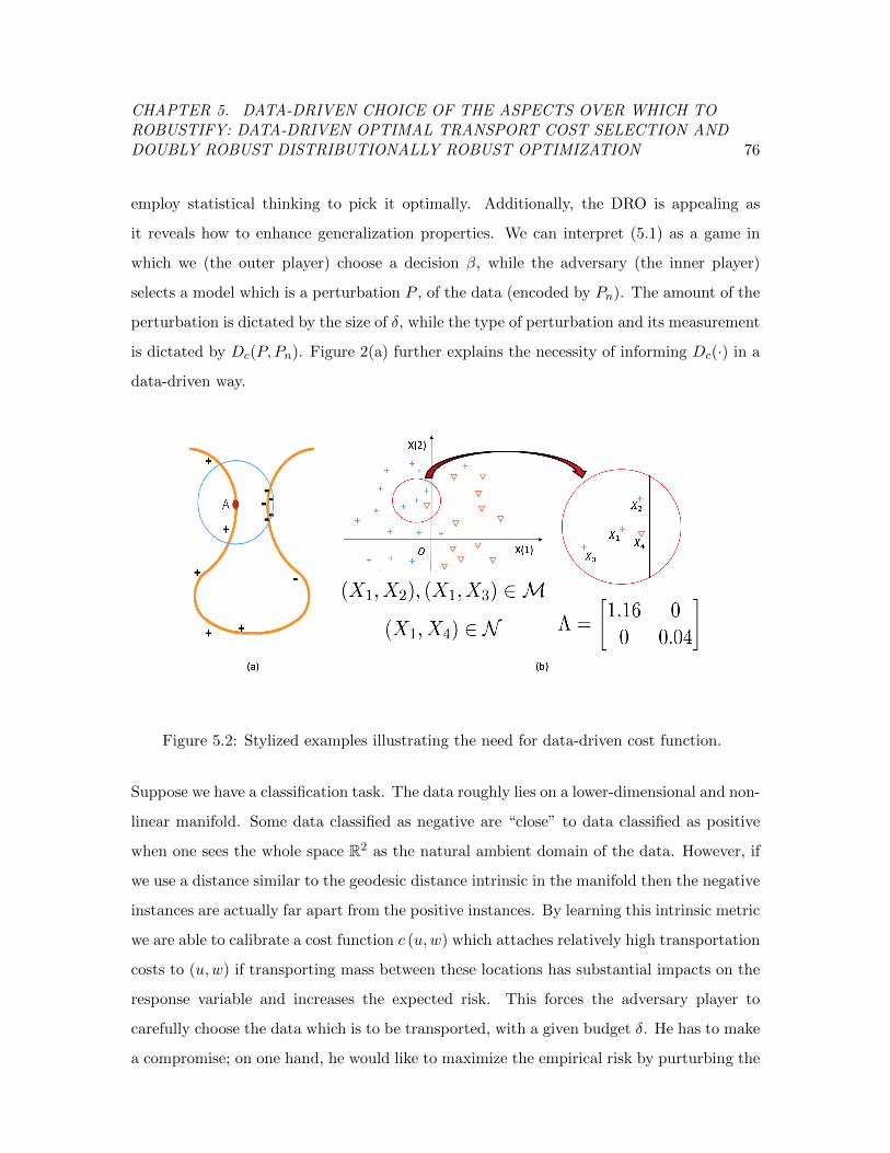
CHAPTER 5. DATA-DRIVEN CHOICE OF THE ASPECTS OVER WHICH TOROBUSTIFY: DATA-DRIVEN OPTIMAL TRANSPORT COST SELECTION ANDDOUBLY ROBUST DISTRIBUTIONALLY ROBUST OPTIMIZATION 76
employ statistical thinking to pick it optimally. Additionally, the DRO is appealing as
it reveals how to enhance generalization properties. We can interpret (5.1) as a game in
which we (the outer player) choose a decision β, while the adversary (the inner player)
selects a model which is a perturbation P , of the data (encoded by Pn). The amount of the
perturbation is dictated by the size of δ, while the type of perturbation and its measurement
is dictated by Dc(P, Pn). Figure 2(a) further explains the necessity of informing Dc(·) in a
data-driven way.
Figure 5.2: Stylized examples illustrating the need for data-driven cost function.
Suppose we have a classification task. The data roughly lies on a lower-dimensional and non-
linear manifold. Some data classified as negative are “close” to data classified as positive
when one sees the whole space R2 as the natural ambient domain of the data. However, if
we use a distance similar to the geodesic distance intrinsic in the manifold then the negative
instances are actually far apart from the positive instances. By learning this intrinsic metric
we are able to calibrate a cost function c (u,w) which attaches relatively high transportation
costs to (u,w) if transporting mass between these locations has substantial impacts on the
response variable and increases the expected risk. This forces the adversary player to
carefully choose the data which is to be transported, with a given budget δ. He has to make
a compromise; on one hand, he would like to maximize the empirical risk by purturbing the
CHAPTER 5. DATA-DRIVEN CHOICE OF THE ASPECTS OVER WHICH TOROBUSTIFY: DATA-DRIVEN OPTIMAL TRANSPORT COST SELECTION ANDDOUBLY ROBUST DISTRIBUTIONALLY ROBUST OPTIMIZATION 77
data between locations that has substantial impacts on the response variable, but on the
other hand he has to pay higher cost for those purturbations. As a result, this compromise
of the DRO procedure leads to the focus on reagions of relevance and hence improves the
generalization performance.
The idea can be further explored in the context of a logistic regression shown in Figure
2(b): Suppose that d = 2, and that Y depends only on X(1), the first coordinate of
X. The metric learning in (5.7) will capture the more informative X(1) in the data and
induce a cost function which bears relatively high transportation cost in X(1) direction
while relatively low transportation cost along X(2) direction. From the standpoint of the
adversarial player, he has to reach a compromise between maximizing the expected loss
(which is his objective) by transporting more along the impactful X(1) direction and paying
a higher cost for perturbing along X(1) direction with his limited budget δ.
5.3 Background on Optimal Transport and Metric Learning
Procedures
This section provides a quick review of basic notions in optimal transport for defining
Dc(P, Pn) and in metric learning for calibrating the cost function c(·).
5.3.1 Defining Optimal Transport Distances and Discrepancies
Assume that the cost function c : Rd+1 × Rd+1 → [0,∞] is lower semicontinuous. We also
assume that c(u, v) = 0 if and only if u = v. Given two distributions P and Q, with supports
SP and SQ, respectively, we define the optimal transport discrepancy, Dc, via
Dc (P,Q) = infEπ [c(U, V )] : π ∈ P
(SP × SQ
), πU = P, πV = Q
, (5.5)
where P(SP ×SQ) is the set of probability distributions π supported on SP×SQ , and πU and
πV denote the two marginals of π. The non-negativeness of c(·) ensures that Dc(P,Q) ≥ 0
and the condition that c(u, v) = 0 if and only if u = v guarantees that Dc(P,Q) = 0 if
and only P = Q. If c(·) is also symmetric (i.e. c(u, v) = c(v, u)), and there exists % ≥ 1
such that c1/%(u,w) ≤ c1/%(u, v) + c1/%(v, w) (i.e. c1/%(·) satisfies the triangle inequality)

CHAPTER 5. DATA-DRIVEN CHOICE OF THE ASPECTS OVER WHICH TOROBUSTIFY: DATA-DRIVEN OPTIMAL TRANSPORT COST SELECTION ANDDOUBLY ROBUST DISTRIBUTIONALLY ROBUST OPTIMIZATION 78
then it can be verified (see Villani (2008)) that D1/%c (P,Q) is a metric. For example, if
c(u, v) = ‖u − v‖%q for q ≥ 1 (where ‖u − v‖q denotes the lq norm in Rd+1) then Dc(·) is
known as the Wasserstein distance of order %. An important observation is that (5.5) is a
linear program in the variable π.
5.3.2 On Metric Learning Procedures
In order to keep the discussion focused, we pick only a few metric learning methods for the
calibration of cost function in DRO formulation, but we emphasize that our approach can
combine with almost any other methods in the metric learning literature. The paper Bellet
et al. (2013) gives a wide survey of various metric learning procedures. The procedures
we employed can already improve significantly upon natural benchmarks, and these metric
families can be related to adaptive regularization. This connection will be useful to further
enhance the intuition of our procedure.
5.3.2.1 The Mahalanobis Distance
The Mahalanobis metric is defined as
dΛ
(x, x′
)=((x− x′
)TΛ(x− x′
))1/2,
where Λ is symmetric and positive semi-definite and we write Λ ∈ PSD. Note that dΛ(x, x′)
is the metric induced by the norm ‖x‖Λ =√xTΛx.
Suppose our data is of the form Dn = (Xi, Yi)ni=1 and Yi ∈ −1,+1. The prediction
variables are assumed to have already been standardized. Motivated by applications such
as social networks, where there is a natural graph connecting instances in the data, and the
information of connection is summarized in setsM and N , whereM is the set of the pairs
that should be close (so that we can connect them) to each other, while N characterizes
the relations that the pairs should be far away (not connected). They are often called side
information of the data. We define them as
M := (Xi, Xj) | Xi and Xj must connect ,
N := (Xi, Xj) | Xi and Xj should not connect .

CHAPTER 5. DATA-DRIVEN CHOICE OF THE ASPECTS OVER WHICH TOROBUSTIFY: DATA-DRIVEN OPTIMAL TRANSPORT COST SELECTION ANDDOUBLY ROBUST DISTRIBUTIONALLY ROBUST OPTIMIZATION 79
While it is typically assumed that M and N are given, one may also resort to k-Nearest-
Neighbor (k-NN) method to generate these sets if they are not available. This is the
approach we follow in our numerical experiments. It is worth noting that the choice of any
criterion for the definition of M and N should be oriented by the learning task so as to
achieve both interpretability and performance.
In our experiments we assign the pair (Xi, Xj) to M if they are sufficiently close in the
k-NN criterion, and with the same label Yi = Yj . Else if Yi 6= Yj , we assign them to N .
The work of Xing et al. (2002), one of pioneer paper on this subject, suggests to solve the
following optimization problem
minΛ∈PSD
∑(Xi,Xj)∈M
d2Λ (Xi, Xj) (5.6)
s.t.∑
(Xi,Xj)∈N
d2Λ (Xi, Xj) ≥ λ. (5.7)
to achieve the goal of minimizing the total distance between pairs that should be connect,
while keeping the pairs that should not connect well separated. The constant λ > 0 is not
essential, since Λ can be normalized by λ and we can choose λ = 1 without loss of generality.
The optimization problem (5.7) is a typical semidefinite programming and has been widely
studied, see, for example, Xing et al. (2002) for a projection-based algorithm; and Schultz
and Joachims (2004) for a factorization-based procedure; or the survey paper Bellet et al.
(2013) for comparison between various algorithms.
We have chosen formulation (5.7) to estimate Λ as it is most intuitive, while more advanced
metric learning techniques developed recently can also be incorporated into the estimation
of cost function c(·) for our DRO formulation. (see Li et al. (2016)).
5.3.2.2 Using Mahalanobis Distance in Data-Driven DRO
Just as before assume that the underlying data takes the form Dn = (Xi, Yi)ni=1, where
Xi ∈ Rd and Yi ∈ R and the loss function, depending on a decision variable β ∈ Rm, is
given by l(x, y, β). Note that no linear structure is imposed on the underlying model or on
the loss function. Analogous to the cost function c(·) in (5.4), here we define a cost function

CHAPTER 5. DATA-DRIVEN CHOICE OF THE ASPECTS OVER WHICH TOROBUSTIFY: DATA-DRIVEN OPTIMAL TRANSPORT COST SELECTION ANDDOUBLY ROBUST DISTRIBUTIONALLY ROBUST OPTIMIZATION 80
cΛ(·) associated with a positive semidefinite matrix Λ as
cΛ
((x, y), (x′, y′)
)= d2
Λ
(x, x′
)I(y = y′
)+∞I
(y 6= y′
). (5.8)
The infinite contribution in the definition of cΛ (i.e. the∞·I (y 6= y′) part) indicates that the
adversarial player in the DRO formulation is not allowed to perturb the response variable.
Since the sets M and N depend on Wi = (Xi, Yi), the cost function cΛ(·) will be informed
by the Yi’s. With this data-driven cost function at hand we can then estimate β via
minβ
supP :DcΛ (P,Pn)≤δ
E[l(X,Y, β)]. (5.9)
It is worth noting that Λ comes only into the definition of the cost function.
5.3.2.3 Mahalanobis Metrics on a Non-Linear Feature Space
In this subsection, we consider the case when the cost function is defined on non-linear
transformed data. Assume that the data takes the form Dn = (Xi, Yi)ni=1, where Xi ∈ Rd
and Yi ∈ R and the loss function, depending on decision variable β ∈ Rm, is given by
l (x, y, β). We define
cΦΛ
((x, y), (x′, y′)
)= d2
Λ
(Φ (x) ,Φ
(x′))I(y = y′
)+∞I
(y 6= y′
), (5.10)
for Λ ∈ PSD. To preserve the properties of a cost function (i.e. non-negativity, lower
semicontinuity and cΦΛ (u,w) = 0 implies u = w), we assume that Φ (·) is continuous and
that Φ (w) = Φ (u) implies that w = u. Then we can apply a metric learning procedure,
such as the one described in (5.7), to calibrate Λ.
5.4 Data Driven Cost Selection and Adaptive Regularization
In this section we establish a direct connection between our fully data-driven DRO procedure
and adaptive regularization. Our main result also reveals a direct connection between the
metric learning and adaptive regularized estimators.
Throughout this section we consider a data set of the form Dn = (Xi, Yi)ni=1 with Xi ∈ Rd

CHAPTER 5. DATA-DRIVEN CHOICE OF THE ASPECTS OVER WHICH TOROBUSTIFY: DATA-DRIVEN OPTIMAL TRANSPORT COST SELECTION ANDDOUBLY ROBUST DISTRIBUTIONALLY ROBUST OPTIMIZATION 81
and Yi ∈ R as before. With the cost function cΛ(·) defined in (5.8), we have the following
results. Its proof is given in the Appendix.
Theorem 5.1 (DRO Representation for Generalized Adaptive Regularization). Assume
that Λ ∈ Rd×d in (5.8) is positive definite and the loss function is mean squared error, we
have the following representation
minβ
maxP :DcΛ (P,Pn)≤δ
E1/2P
[(Y −XTβ
)2]= min
β
√√√√ 1
n
n∑i=1
(Yi −XT
i β)1/2
+√δ ‖β‖Λ−1 . (5.11)
Moreover in the context of adaptive regularized logistic regression with Y ∈ −1,+1 , we
have
minβ
maxP :DcΛ (P,Pn)≤δ
E[log(
1 + e−Y (XT β))]
= minβ
1
n
n∑i=1
log(
1 + e−Yi(XTi β))
+ δ ‖β‖Λ−1 .(5.12)
In particular, when Λ is a diagonal positive definite matrix, we recover a more familiar
version of (5.11) for adaptive regularization:
minβ
maxP :DcΛ (P,Pn)≤δ
E1/2P
[(Y −XTβ
)2]= min
β
√√√√ 1
n
n∑i=1
(Yi −XT
i β)2
+√δ
√√√√ d∑i=1
β2i /Λii.(5.13)
The adaptive regularization method was initially derived as a generalization of ridge regres-
sion in Hoerl and Kennard (1970b) and Hoerl and Kennard (1970a). Recent work shows
that adaptive regularization can improve the prediction power of its non-adaptive coun-
terpart, especially in high-dimensional settings (see in Zou (2006) and Ishwaran and Rao
(2014)).
In view of (5.13), our discussion in Section 5.3.2.1 uncovers tools which can be used to esti-
mate the coefficients 1/Λii : 1 < i ≤ d. To complement the intuition given in Figure 1(b),
note that in the adaptive regularization literature one often choose Λii ≈ 0 to force βi ≈ 0
(i.e., there is a high penalty to variables with low explanatory power). This corresponds to
the low transport costs along those low explanatory directions in our DRO formulation.

CHAPTER 5. DATA-DRIVEN CHOICE OF THE ASPECTS OVER WHICH TOROBUSTIFY: DATA-DRIVEN OPTIMAL TRANSPORT COST SELECTION ANDDOUBLY ROBUST DISTRIBUTIONALLY ROBUST OPTIMIZATION 82
5.5 Solving Data Driven DRO Based on Optimal Transport
Discrepancies
To fully take advantage of the synergies between DRO and metric learning it is crucial to
have an algorithm efficiently estimating β from (5.1). In the presence of a special represen-
tation such as (5.2) or (5.13), we can apply standard stochastic optimization methods (see
Lei and Jordan (2016)).
Our objective in this section is to give algorithms which are applicable to more general loss
and cost functions, when a simplified representation is not accessible.
Throughout this section the data has the form Dn = (Xi, Yi)ni=1 ⊂ Rd+1. The loss func-
tion is written as l (x, y, β) : (x, y) ∈ Rd+1, β ∈ Rm. We assume that for each (x, y), the
function l (x, y, ·) is convex and continuously differentiable. Further, we shall consider cost
functions of the form
c((x, y) ,
(x′, y′
))= c
(x, x′
)I(y = y′
)+∞I
(y 6= y′
),
as this will simplify the form of the dual representation in the inner optimization of our
DRO formulation. To ensure boundedness of the DRO formulation, we impose the following
assumption.
Assumption 1. There exists Γ(β, y) ∈ (0,∞) such that l(u, y, β) ≤ Γ(β, y) · (1 + c(u, x)),
for all (x, y) ∈ Dn, Under Assumption 1, we can guarantee that
maxP :Dc(P,Pn)≤δ
EP [l (X,Y, β)] ≤ (1 + δ) maxi=1,...,n
Γ (β, Yi) <∞.
Using the strong duality theorem for semi-infinity linear programming problem in Appendix
B of Blanchet et al. (2016a),
maxP :Dc(P,Pn)≤δ
EP [l (X,Y, β)] = minλ≥0
1
n
n∑i=1
φ (Xi, Yi, β, λ) , (5.14)
where ψ(u,X, Y, β, λ) := l(u, Y, β)−λ(c(u,X)−δ), φ (X,Y, β, λ) := maxu∈Rd ψ(u,X, Y, β, λ).
Therefore,
minβ
maxP :DcΛ (P,Pn)≤δ
EP [l (X,Y, β)] = minλ≥0,β
EPn [φ (X,Y, β, λ)] . (5.15)

CHAPTER 5. DATA-DRIVEN CHOICE OF THE ASPECTS OVER WHICH TOROBUSTIFY: DATA-DRIVEN OPTIMAL TRANSPORT COST SELECTION ANDDOUBLY ROBUST DISTRIBUTIONALLY ROBUST OPTIMIZATION 83
The right hand side of (5.15) is minimized over β and λ, to which we can apply stochastic
approximation algorithms if the gradient of φ (·) with respect to β and λ exist. However, φ (·)
itself is given by solving a maximization problem, so its gradient is not readily accessible.
Therefore we consider a smoothing approximation technique to remove the maximization
problem in φ (·).
The smoothing approximation for φ (·) is defined as,
φε,f (X,Y, β, λ) = ε log
(∫Rd
exp ([ψ (u,X, Y, β, λ)] /ε) f (u) du
),
where f (·) is a probability density in Rd; for example, f can be taken as the density of a
normal distribution and ε > 0 is a smoothing parameter.
Theorem 5.1 below quantifies the error due to smoothing approximation.
Lemma 5.1. Under mild technical assumptions (see Assumption 1-4 in Appendix 5.9.2),
there exists ε0 > 0 such that for every ε < ε0, we have
φ(X,Y, β, λ) ≥ φε,f (X,Y, β, λ) ≥ φ(X,Y, β, λ)− dε log(1/ε)
The proof of Lemma 5.1 is given in Appendix 5.9.2.
With the help of smooth approximation we transform the original optimization problem
to a standard stochastic optimization problem and we can solve it by mini-batch based
stochastic approximation (SA) algorithm. Notice that the gradient of φε,f (·), as a function
and β and λ, satisfies
∇βφε,f (X,Y, β, λ) =EU∼f [exp (ψ (U,X, Y, β, λ) /ε)∇βl (U,X, Y )]
EU∼f [exp (ψ (U,X, Y, β, λ) /ε)], (5.16)
∇λφε,f (X,Y, β, λ) =EU∼f [exp (ψ (U,X, Y, β, λ) /ε) (δ − cΛn (U,X))]
EU∼f [exp (ψ (U,X, Y, β, λ) /ε)]. (5.17)
which is still in the form of expectation, but we can approximate the gradient by a simple
Monte Carlo sampling, i.e., we sample Ui’s from f(·) and evaluate the numerators and
denominators of the gradient using Monte Carlo separately. The details of this SA algorithm
are given in Algorithm 2.

CHAPTER 5. DATA-DRIVEN CHOICE OF THE ASPECTS OVER WHICH TOROBUSTIFY: DATA-DRIVEN OPTIMAL TRANSPORT COST SELECTION ANDDOUBLY ROBUST DISTRIBUTIONALLY ROBUST OPTIMIZATION 84
Algorithm 2 Stochastic Gradient Descent with Continuous State
1: Initialize λ = 0, and β to be empirical risk minimizer, ε = 0.5, tracking error Error =
100.
2: while Error > 10−3 do
3: Sample a mini-batch Xj , YjMj=1 uniformly from n observations , with M ≤ n.
4: For each j = 1, . . . ,M , sample i.i.d. U (j)k
Lk=1 from N
(0, σ2Id×d
).
5: We denote f jL as empirical distribution for U(j)k ’s, and estimate the batched as
∇βφε,f =1
M
M∑j=1
∇βφε,fjL (Xj , Yj , β, λ) ,∇λφε,f =1
M
M∑j=1
∇λφε,fjL (Xj , Yj , β, λ) .
6: Update β and λ using β = β − αβ∇βφε,f and λ = λ− αλ∇λφε,f .
7: Update tracking error Error as the norm of difference between latest parameter and
average of last 50 iterations.
8: Output β.
Remark 5.1. The above optimization problem can be written as a mixed problem in the
sense of J.Blanchet et al. (2017)
minλ≥0,β
1
n
n∑i=1
ε log(EU [exp(ψ(U,Xi, Yi, β, λ)/ε)]) =: minλ≥0,β
1
n
n∑i=1
Φi(EU [ΨU (β, λ)]) =: minλ≥0,β
F (β, λ),
(5.18)
where
ΨU (β, λ) :=(
exp(ψ(U,X1, Y1, β, λ)/ε), · · · , exp(ψ(U,XM , YM , β, λ)/ε))T,
and Φi(EU [ΨU (β, λ)]) := ε log(EU [exp(ψ(U,Xi, Yi, β, λ)/ε)]) = φε,f (Xi, Yi, β, λ) .
Let θ := (β, λ)T , then exp ([ψ (u,X, Y, θ)] /ε) f (u) is log-convex in θ for all u ∈ R, and by
Boyd and Vandenberghe (2004) p.106 the function φε,f is convex in θ, so F is also convex.
Remark 5.2. Note that
∇βφε,f (X,Y, β, λ) =EU∼f [exp (ψ (U,X, Y, β, λ) /ε)∇βl (U,X, Y )]
EU∼f [exp (ψ (U,X, Y, β, λ) /ε)]
relates to the quotient of two expectations. In general,∑Lk=1 exp (ψ (Uk, X, Y, β, λ) /ε)∇βl (Uk, X, Y )∑L
k=1 exp (ψ (Uk, X, Y, β, λ) /ε)
CHAPTER 5. DATA-DRIVEN CHOICE OF THE ASPECTS OVER WHICH TOROBUSTIFY: DATA-DRIVEN OPTIMAL TRANSPORT COST SELECTION ANDDOUBLY ROBUST DISTRIBUTIONALLY ROBUST OPTIMIZATION 85
is not an unbiased estimator for ∇βφε,f (X,Y, β, λ). The unbiased estimator ∇βφε,fjL (Xj , Yj , β, λ)
can be construncted via multi-level randomization, see Blanchet and Glynn (2015). ∇λφε,fis analogue.
Remark 5.3. Let θ = (β, λ)T and define
h(Xj , Yj , (U(j)k )Lk=1, θ) := ∇θφε,fjL (Xj , Yj , θ)
and
H(Z, θ) :=1
M
M∑j=1
h(Xj , Yj , (U(j)k )Lk=1, θ),
where Z = ((Xj , Yj , (U(j)k )Lk=1)Mj=1). We have E[H(Z, θ)|θ] = EPM
⊗Pf [∇θφε,f (X,Y, U, θ)|θ],
where PM is the empirical measure formed by the M data points, and Pf denotes the distri-
bution of U . Thus, Algorithm 2 can be seen as a special type of stochastic gradient descend
algorithm.
Theorem 5.2. Let θ∗ = (β∗, λ∗)T be an optimal value for minθ F (θ) in (5.18). Assume
that i) the problem is optimized over a compact and convex set Θ which contains θ∗ and
(θt)t≥0 generated by the algorithm, ii) Inside the compact set Θ both the loss function l(·)
and the cost function c(·) are twice continously differentiable, Then
a) If F is µ-strongly convex, when taking step-size αt = 2µ√t
we then have
E[‖θT − θ∗‖22] ≤ 4C
µ2(T + 1),
where C is some constant.
b) If F is just convex but we can find some constant D such that E[‖θt − θ∗‖22] ≤ D for all
t ≥ 0, when taking step-size αt = 2√t+1
we then have
E[F (θT )]− F (θ∗) ≤ 2√
2(C +D)√T
,
where C is some constant.
Proof. Since both the loss function l(·) and the cost function c(·) are twice continously
differentiable and the set Θ is compact, so the functions Φi and ΨU are also twice continously
differentiable and their gradients are L-Lipschitz continuous for some constant L. Therefore,
it satisfies all the assumptions in J.Blanchet et al. (2017) and the results follow.

CHAPTER 5. DATA-DRIVEN CHOICE OF THE ASPECTS OVER WHICH TOROBUSTIFY: DATA-DRIVEN OPTIMAL TRANSPORT COST SELECTION ANDDOUBLY ROBUST DISTRIBUTIONALLY ROBUST OPTIMIZATION 86
Remark 5.4. As shown in Remark 5.1 F is convex, but if F is not strongly convex we can
generally add a penalty term ‖θ‖22 to make it strongly convex.
5.6 Robust Metric Learning
The objective of this section is to explore how to learn data-driven cost function cΛ in a
robust way and combine it with our DD-DRO model. We call this new model Doubly Ro-
bust Data-Driven Distributionally Robust Optimization (DD-R-DRO). Robust optimization
(RO) is a family of optimization techniques that deals with uncertainty or misspecification
in the objective function and constraints. It was first proposed in Ben-Tal et al. (2009) and
has attracted increasing attentions in the recent decades El Ghaoui and Lebret (1997) and
Bertsimas et al. (2011). It has been applied in machine learning to regularize statistical
learning procedures, for example, in Xu et al. (2009a) and Xu et al. (2009b) robust opti-
mization was employed for SR-Lasso and support vector machines. Note that the classical
robust optimization is different from our distributionally robust optimization in the sense
that classical robust optimization concerns only deterministic uncertain scenarios and we
will apply this classical robust optimization only to the cost function learning procedure in
our DD-DRO. The reason that we want to learn the cost function in a robust way is due to
the fact that there often exists noisiness or incorrectness in side information (e.g. the train-
ing constraint sets M and N or the relative constraints R defined later, are often gained
from customers’ implicit feedback, and are quite noisy.) This extra layer of robustness will
reduce the variability in testing error as it is shown in the later numerical experiments.
5.6.1 Robust Optimization for Relative Metric Learning
The robust metric learning we shall use is based on the work of Huang et al. (2012). Consider
the relative constraint set R containing data triplets with relative relation defined as
R = (i, j, k) |dΛ(Xi, Xj) should be smaller than dΛ(Xi, Xk) .
and the Relative Metric Learning formulation
minΛ0
∑(i,j,k)∈R
(d2
Λ (Xi, Xj)− d2Λ (Xi, Xk) + 1
)+. (5.19)

CHAPTER 5. DATA-DRIVEN CHOICE OF THE ASPECTS OVER WHICH TOROBUSTIFY: DATA-DRIVEN OPTIMAL TRANSPORT COST SELECTION ANDDOUBLY ROBUST DISTRIBUTIONALLY ROBUST OPTIMIZATION 87
Suppose we know that about 1 − α ∈ (0, 1] of the constraints are noisy (the value of α is
usually given by experience or it can also be inferred by cross validation), but we cannot
determine exactly which part of them are noisy. Instead of optimizing over all subsets of
constraints, we try to minimize the worst case loss function over all possible α |R| constraints
(where |·| denote the cardinality of a set) and obtain the following min-max formulation
minΛ0
maxq∈T (α)
∑(i,j,k)∈R
qi,j,k(d2
Λ (Xi, Xj)− d2Λ (Xi, Xk) + 1
)+, (5.20)
where T (α) is a robust uncertainty set of the form
T (α) =q = qi,j,k|(i, j, k) ∈ R |0 ≤ qi,j,k ≤ 1,
∑(i,j,k)∈R
qi,j,k ≤ α× |R|,
which is a convex and compact set.
Firstly we observe that the above minimax problem is equivalent to
minΛ0
maxq∈T (α)
∑(i,j,k)∈R
qi,j,k(d2
Λ (Xi, Xj)− d2Λ (Xi, Xk) + 1
), (5.21)
because qi,j,k = 0 whenever d2Λ (Xi, Xj) − d2
Λ (Xi, Xk) + 1 < 0. So our algorithm will be
quite different from the original algorithm proposed by Huang et al. (2012) in the sense that
our alorithm doesn’t resort to any smooth technique, instead we will use the primal-dual
steepest descent algorithm.
Secondly, the objective function in (5.21) is convex in Λ and concave (linear) in q. Define
L(Λ, q) :=∑
(i,j,k)∈R
qi,j,k(d2
Λ (Xi, Xj)− d2Λ (Xi, Xk) + 1
)+κ
2‖Λ‖2F , (5.22)
where κ > 0 is the tuning parameter and ‖ · ‖F denote the Frobenius norm. In addition we
define
f(Λ) := maxq∈T (α)
L(Λ, q), g(q) := minΛ0
L(Λ, q) (5.23)
and since L is strongly convex in Λ and linear in q we also have
q(Λ) := arg maxq∈T (α)
L(Λ, q), Λ(q) := arg minΛ0
L(Λ, q) (5.24)
Our iterative algorithm uses the fact that f(Λ) and q(Λ) can actually be fast obtained by
a simple sorting: for a fixed Λ 0, the inner maximization is linear in q, and the optimal

CHAPTER 5. DATA-DRIVEN CHOICE OF THE ASPECTS OVER WHICH TOROBUSTIFY: DATA-DRIVEN OPTIMAL TRANSPORT COST SELECTION ANDDOUBLY ROBUST DISTRIBUTIONALLY ROBUST OPTIMIZATION 88
q satisfy qi,j,k = 1 whenever (dΛ (Xi, Xj)− dΛ (Xi, Xk) + 1) ≥ 0 and ranks in the top α |R|
largest values and set qi,j,k = 0 otherwise. If there are more than one optimal q’s, break
the tie by choosing q(Λ) := arg maxq∈T (α) L(Λ, q)− κ‖q− q(n)‖22 at the (n+ 1)-th iteration,
where κ is a tuning parameter that is small enough such that it ensures that the q(Λ) is
chosen among the all the optimal ones. On the other hand, since L(Λ, q) is smooth in Λ,
we can also obtain g(q) and Λ(q) fast by gradient descent.
We summarize the primal-dual steepest descent algorithm as in Algorithm 3.
5.6.2 Robust Optimization for Absolute Metric Learning
The RO formulation of (5.7) that we present here appears to be novel in the literature.
First we write (5.7) in its Lagrangian form,
minΛ0
maxλ≥0
∑(i,j)∈M
d2Λ (Xi, Xj) + λ
(1−
∑(i,j)∈N
d2Λ (Xi, Xj)
). (5.25)
Similar to R, the side information sets M and N often suffer from noisiness or inaccuracy
as well. Let us assume that about 1 − α proportion of the constraints in M and N are,
respectively, inaccurate. We then construct robust uncertainty sets W(α) and V(α) from
M and N as
W(α) =η = ηij : (i, j) ∈M |0 ≤ ηij ≤ 1,
∑(i,j)∈M
ηij ≤ α× |M|,
V(α) =ξ = ξij : (i, j) ∈ N |0 ≤ ξij ≤ 1,
∑(i,j)∈N
ξij ≥ α× |N |.
Then the RO formulation of (5.25) can be written as
minΛ0
maxλ≥0
maxη∈W(α),ξ∈V(α)
∑(i,j)∈M
ηi,jd2Λ (Xi, Xj) + λ
(1−
∑(i,j)∈N
ξi,jd2Λ (Xi, Xj)
)(5.26)
The switch of maxλ with max(η,ξ) is valid in general. Note also that the Cartesian product
M (α)×N (α) is a compact set, and the objective function is convex in Λ and concave (lin-
ear) in pair (η, ξ), so we can further apply Sion’s min-max Theorem again (see in Terkelsen
(1973)) to switch the order of minΛ-max(η,ξ). This leads to an iterative algorithm.
Define q := (η, ξ) as the dual variable and
L(Λ, q) :=∑
(i,j)∈M
ηi,jd2Λ (Xi, Xj) + λ
(1−
∑(i,j)∈N
ξi,jd2Λ (Xi, Xj)
)+κ
2‖Λ‖2F , (5.27)

CHAPTER 5. DATA-DRIVEN CHOICE OF THE ASPECTS OVER WHICH TOROBUSTIFY: DATA-DRIVEN OPTIMAL TRANSPORT COST SELECTION ANDDOUBLY ROBUST DISTRIBUTIONALLY ROBUST OPTIMIZATION 89
Algorithm 3 Sequential Coordinate-wise Metric Learning Using Relative Relations
1: Initialize Set the iteration counter n = 0, the positive definite matrix Λ = Id, and
the tolerance ε = 10−3. Then randomly sample α proportion of elements from R to
construct q.
2: (Optimal test) Terminate if
|minf(Λ(n)), f(Λ(q(n))) −maxg(q(n)), g(q(Λ(n)))| ≤ ε.
and Output
Λ = arg minf(Λ)|Λ = Λ(n) or Λ = Λ(q(n))
q = arg maxg(q)|q = q(n) or q = q(Λ(n)),
3: (Line search) Generate the intermediate Λ(n+1), q(n+1) with perfect line search
Λ(n+1) = (1− γn)Λ(n) + γnΛ(q(Λ(n)))
q(n+1) = (1− βn)q(n) + βnq(Λ(q(n))),
where
γn = arg minγ∈[0,1]
f((1− γ)Λ(n) + γΛ(q(Λ(n)))
)βn = arg max
β∈[0,1]g((1− β)q(n) + βq(Λ(q(n)))
),
4: (Update the iterates)
Λ(n+1) = arg minf(Λ)|Λ = Λ(n+1) or Λ = Λ(q(n))
q(n+1) = arg maxg(q)|q = q(n+1) or q = q(Λ(n)),
and then return to Step 2 with counter n← n+ 1.
CHAPTER 5. DATA-DRIVEN CHOICE OF THE ASPECTS OVER WHICH TOROBUSTIFY: DATA-DRIVEN OPTIMAL TRANSPORT COST SELECTION ANDDOUBLY ROBUST DISTRIBUTIONALLY ROBUST OPTIMIZATION 90
and
f(Λ) := maxq∈T (α)
L(Λ, q), g(q) := minΛ0
L(Λ, q) (5.28)
and
q(Λ) := arg maxq∈T (α)
L(Λ, q), Λ(q) := arg minΛ0
L(Λ, q) (5.29)
Similarly, the f(Λ) and q(Λ) are easy to obtain. At the n-th step, given fixed Λ(n−1) 0
and λ > 0 (it is easy to observe that optimal solution λ is positive, i.e. the constraint is
active so we may safely assume λ > 0), the inner maximization problem looks like,
maxη∈W(α)
∑(i,j)∈M
ηi,jd2Λ(n−1) (Xi, Xj) + λ
(1− min
ξ∈V(α)
∑(i,j)∈N
ξi,jd2Λ(n−1) (Xi, Xj)
).
Analogous to the relative constraints case, the optimal η and ξ satisfy: ηi,j is 1, if d2Λ(n−1) (Xi, Xj)
ranks top α withinM and equals 0 otherwise; while ξi,j = 1 if d2Λ(n−1) (Xi, Xj) ranks bottom
α within N and equals 0 otherwise. So we also defineMα(Λ(n−1)) as a subset ofM, which
contains the constraints with largest α percent of dΛ(n−1) (·); and define Nα(Λ(n−1)) as a
subset of N , which contains the constraints with smallest α percent of dΛ(n−1) (·). Then the
optimal solution given fixed Λ(n−1) can be reformulated as ηi,j = 1 if (i, j) ∈ Mα(Λ(n−1))
and ξi,j = 1 if (i, j) ∈ Nα(Λ(n−1)).
On the other hand, given fixed η and ξ, we can simplify the minimization problem g(q) as
minΛ0
∑(i,j)∈Mα(Λ(n−1))
d2Λ (Xi, Xj) s.t.
∑(i,j)∈Nα(Λ(n−1))
d2Λ (Xi, Xj) ≥ 1.
This formulation of the minimization problem g(q) takes the same form as (5.7) and it thus
can be solved by similar SDP algorithms presented in Xing et al. (2002). On the whole we
solve the minimax problem of (5.26) by using the same primal-dual algorithm as presented
in Algorithm 3.
Other robust methods have also been considered in the metric learning literature, see Zha
et al. (2009) and Lim et al. (2013) although the connections to RO are not fully exposed.
Theorem 5.3. There exists saddle points (Λ, q) for the minimax problems (5.22) and (5.27)
respectively. The Algorithm 3 converges linearly to the common optimal value f(Λ) = g(q)

CHAPTER 5. DATA-DRIVEN CHOICE OF THE ASPECTS OVER WHICH TOROBUSTIFY: DATA-DRIVEN OPTIMAL TRANSPORT COST SELECTION ANDDOUBLY ROBUST DISTRIBUTIONALLY ROBUST OPTIMIZATION 91
in the sense that
f(Λ(n+1))− f(Λ) ≤ θ(f(Λ(n))− f(Λ)
)g(q(n+1))− g(q) ≤ θ
(g(q(n))− g(q)
),
where θ ∈ (0, 1) is some constant and the functions f and g are define by (5.23) and (5.28)
respectively.
Proof. In both (5.22) and (5.27) the function L is strongly convex in Λ and q takes value
in a bounded set, so it satisfies the condition of existence of saddle points, see Zhu (1994)
and R.T.Rockafeller (1970). Note that though L is not strongly concave in q but it is linear
in q. At iteration n + 1 if there are more than one optimal values of q we can use the
proximal point algorithm to create a strongly convex-concave Lagrangian, i.e. we maximize
−‖q−q(n)‖22 to break the tie. The linear convergence follows then from Theorem 3.3 in Zhu
(1994).
5.7 Numerical Experiments
5.7.1 Numerical Experiments for DD-DRO
We validate our data-driven cost function based DRO on 5 real data sets from the UCI
machine learning database Lichman (2013). We focus on a DRO formulation for a linear
classification model with the log-exponential loss. We use the linear metric learning frame-
work (5.7) to learn a positive semidefinite matrix Λ and then plug it into the cost function
cΛ defined in (5.8). We denote this model DRO-L. In addition, we also fit a cost function
cΦΛ to the quadratric transformed data, as explained in (5.10); the model is denoted by
DRO-NL. We compare our DRO-L and DRO-NL with logistic regression (LR), and regu-
larized logistic regression (LRL1). For each iteration and each data set, the data is split
randomly into training and test sets. We fit the models on the training set and evaluate the
performance on test set. The regularization parameter is chosen via 5−fold cross-validation
for LRL1, DRO-L and DRO-NL. For each data set, we perform 200 independent experi-
ments and report the mean and standard deviation for the training error, testing error and

CHAPTER 5. DATA-DRIVEN CHOICE OF THE ASPECTS OVER WHICH TOROBUSTIFY: DATA-DRIVEN OPTIMAL TRANSPORT COST SELECTION ANDDOUBLY ROBUST DISTRIBUTIONALLY ROBUST OPTIMIZATION 92
testing accuracy. The details of the numerical results and basic information of the data are
summarized in Table 5.1.
Table 5.1: Numerical Results for DD-DRO on Real Data Sets.
breast cancer qsar magic minibone spambase
LR
Train 0± 0 .026± .008 .213± .153 0± 0 0± 0
Test 8.75± 4.75 35.5± 12.8 17.8± 6.77 18.2± 10.0 14.5± 9.04
Accur .762± .061 .701± .040 .668± .042 .678± .059 .789± .035
LRL1
Train .185± .123 .614± .038 .548± .087 .401± .167 .470± .040
Test .428± .338 .755± .019 .610± .050 .910± .131 .588± .140
Accur .929± .023 .646± .036 .665± .045 .717± .041 .811± .034
DRO-L
Train .022± .019 .402± .039 .469± .064 .294± .046 .166± .031
Test .126± .034 .557± .023 .571± .043 .613± .053 .333± .018
Accur .954± .015 .733± .026 .727± .039 .714± .032 .887± .011
DRO-NL
Train .032± .015 .339± .044 .381± .084 .287± .049 .195± .034
Test .119± .044 .554± .032 .576± .049 .607± .060 .332± .015
Accur .955± .016 .736± .027 .730± .043 .716± .054 .889± .009
Num Predictors 30 30 10 20 56
Train Size 40 80 30 30 150
Test Size 329 475 9990 125034 2951
5.7.2 Numerical Experiments for DD-R-DRO
In this subsection we proceed to verify the further improved performance of our DD-R-DRO
method on the same five data sets from UCI machine learning data base.
The side information, i.e. the relative constraint set R and the absolute constraint sets M
and N are generated by k-NN method. We then add noisiness to these constraint sets by
randomly replacing the correct constraints with wrong constraints with probability 1− α.
We consider logistic regression (LR), regularized logistic regression (LRL1), DD-DRO with
cost function learned from absolute constraints (DD-DRO (absolute)) and DD-R-DRO(absolute)
with cost function learned from absolute constraints at level of α = 50% and α = 90%; DD-

CHAPTER 5. DATA-DRIVEN CHOICE OF THE ASPECTS OVER WHICH TOROBUSTIFY: DATA-DRIVEN OPTIMAL TRANSPORT COST SELECTION ANDDOUBLY ROBUST DISTRIBUTIONALLY ROBUST OPTIMIZATION 93
DRO with cost function learned from relative constraints (DD-DRO (relative)) and DD-R-
DRO(relative) with cost function learned from relative constraints at level of α = 50% and
α = 90%. For each data and each experiment, we randomly split the data into training and
testing and fit models on training set and evaluate on testing set.
For each data sets, we perform 200 independent experiments and report the mean and stan-
dard deviation of training error, testing error, and testing accuracy. The detailed results
and data set information are summarized in Table 5.2.
After we obtained the learned cost function, we then apply the smoothing approximation
algorithm introduced in Section 5.5 to solve the DRO problem directly, where the size of
uncertainty δ is chosen via 5-fold cross-validation.
We observe that DD-R-DRO presents robust improvement comparing to its non-robust
counterpart DD-DRO when the cost function is learned from noisy side information at level
α = 90%. More important, DD-R-DRO tends to enjoy the variance reduction property due
to RO. In addition, as the robust level increases, i.e. α = 50%, where we believe that the
side information is highly noisy, we observe that the doubly robust based approach seems
to shrink towards to LRL1, and benefits less from the data-driven cost structure.
5.8 Conclusion and Discussion
We have proposed a novel DD-DRO, a fully data-driven DRO procedure, which combines a
semiparametric approach (the metric learning) with a parametric procedure (the expected
loss minimization) and enhances the generalization performance of the underlying para-
metric model. A smoothing technique based algorithm is given for solving the DD-DRO
problem.
Based on DD-DRO we further take noisiness of the side information into account during
the metric learning for the cost function, and introduce robust metric learning method to
DD-DRO, which leads to our DD-R-DRO model. The overall method is then doubly robust;
one is distributionally robustness around the training data, and the other is robust metric
learning of the cost function from the noisy side information. This second layer of robust-
ness not only keeps the improved generalization properties of DD-DRO, but also reduces

CHAPTER 5. DATA-DRIVEN CHOICE OF THE ASPECTS OVER WHICH TOROBUSTIFY: DATA-DRIVEN OPTIMAL TRANSPORT COST SELECTION ANDDOUBLY ROBUST DISTRIBUTIONALLY ROBUST OPTIMIZATION 94
the variability of the testing errors due to the noise in side information.
We emphasize that our approach is applicable to other DRO formulations and is not re-
stricted to classification tasks. Interesting future research avenues which might be worth
considering include the development of a semisupervised framework as in Blanchet and
Kang (2017), in which unlabeled data is used to inform the support of the elements in
Uδ(Pn). Another interesing approach that might be worth exploring is to combine metric
learning for domain adaptation with our DRO model.
5.9 Proof of Main Results
5.9.1 Proof of Theorem 5.1
We first state and prove Lemma 5.2 which will be useful for the proof of Theorem 5.1.
Lemma 5.2. If Λ is a is positive definite matrix and we define ‖x‖Λ =(xTΛx
)1/2, then
‖·‖Λ−1 is the dual norm of ‖·‖Λ. Furthermore, we have
uTw ≤ ‖u‖Λ ‖w‖Λ−1 ,
where the equality holds if and only if, there exists non-negative constant τ , s.t τΛu = Λ−1w
or τΛ−1w = Λu.
Proof of Lemma 5.2. This result is a direct generalization of l2 norm in Euclidean space.
Note that
uTw = (Λu)T (Λ−1w) ≤ ‖Λu‖2∥∥Λ−1w
∥∥2
= ‖u‖Λ ‖w‖Λ−1 . (5.30)
The inequality above is Cauchy-Schwartz inequality for Rd appling to Λu and Λ−1w, and the
equality holds if and only if there exists nonnegative τ , s.t. τΛu = Λ−1w or τΛ−1w = Λu.
By the definition of the dual norm, we have
‖w‖∗Λ = supu:‖u‖Λ≤1
uTw = supu:‖u‖Λ≤1
‖u‖Λ ‖w‖Λ−1 = ‖w‖Λ−1 .
While the first equality follows from the definition of dual norm, the second equality is
due to Cauchy-Schwartz inequality (5.30) and the equality condition therein, and the last
equality are immediate after maximizing.
CHAPTER 5. DATA-DRIVEN CHOICE OF THE ASPECTS OVER WHICH TOROBUSTIFY: DATA-DRIVEN OPTIMAL TRANSPORT COST SELECTION ANDDOUBLY ROBUST DISTRIBUTIONALLY ROBUST OPTIMIZATION 95
Proof of Theorem 5.1. The technique is a generalization of the method used in proving The-
orem 1 in Blanchet et al. (2016a). We can apply the strong duality result (see Proposition 6
in Appendix of Blanchet et al. (2016a)) to the worst-case expected loss function, and obtain
a semi-infinite linear programming problem
supP :DcΛ (P,Pn)≤δ
EP[(Y −XTβ
)2]= min
γ≥0
γδ − 1
n
n∑i=1
supu
(yi − uTβ
)2 − γ ‖xi − u‖2Λ.
For the inner suprema , let us denote ∆ = u−Xi and ei = Yi−XTi β for notation simplicity.
The inner optimization problem associated with (Xi, Yi) becomes,
supu
(yi − uTβ
)2 − γ ‖xi − u‖2Λ= e2
i + sup∆
(∆Tβ
)2 − 2ei∆Tβ − γ ‖∆‖2Λ
,
= e2i + sup
∆
∑
j
|∆j | |βj |
2
+ 2 |ei|∑j
|∆j | |βj | − γ ‖∆‖2Λ
,
= e2i + sup
‖∆‖Λ
‖∆‖2Λ ‖β‖
2Λ−1 + 2 |ei| ‖∆‖Λ ‖β‖Λ−1 − γ ‖∆‖2Λ
,
=
e2i
γ
γ−‖β‖2Λ−1
if γ > ‖β‖2Λ−1 ,
+∞ if γ ≤ ‖β‖2Λ−1 .
While the first equality is due to the change of variable, the second equality follows from
the fact that the last term only depends on the magnitude rather than sign of ∆, so the
maximization problem will always pick a ∆ that satisfies the equality. The third equality
follows from the same reason; we can first apply the Cauchy-Schwartz inequality in Lemma
5.2 and the maximization problem will pick a ∆ satisfying the equality constraint. The last
equality following simply from the first order condition of optimality.
For the outer minimization problem over γ, as the inner suprema equal infinity if γ ≤

CHAPTER 5. DATA-DRIVEN CHOICE OF THE ASPECTS OVER WHICH TOROBUSTIFY: DATA-DRIVEN OPTIMAL TRANSPORT COST SELECTION ANDDOUBLY ROBUST DISTRIBUTIONALLY ROBUST OPTIMIZATION 96
‖β‖2Λ−1 , the worst-case expected loss becomes,
supP :DcΛ (P,Pn)≤δ
EP[(Y −XTβ
)2](5.31)
= minγ>‖β‖2
Λ−1
γδ − 1
n
n∑i=1
(Yi −XT
i β) γ
γ − ‖β‖2Λ−1
,
=
√√√√ 1
n
n∑i=1
(Yi −XT
i β)
+√δ ‖β‖Λ−1
2
.
We see that the objective function on the right hand side of (5.31) is convex and differentiable
and the value function will be infinity as γ → ∞ and γ → ‖β‖2Λ. Solving γ through the
first order condition of optimality, it is straightforward to obtain the last equality in (5.31).
By taking square root on both sides, we proved the claim for the case of mean-squared loss
function.
For the log-exponential loss function the proof is analogous. By applying strong duality
results of semi-infinity linear programming problem in Blanchet et al. (2016a), we can write
the worst case expected loss function as
supP :DcΛ (P,Pn)≤δ
EP[log(1 + exp
(−Y βTX
))]= min
γ≥0
γδ − 1
n
n∑i=1
supu
log(1 + exp
(−YiβTu
))− γ ‖Xi − u‖Λ
.
For each i, we can use Lemma 1 in Shafieezadeh-Abadeh et al. (2015) and dual-norm result
in Lemma 5.2 to deal with the inner maximization problem and obtain
supu
log(1 + exp
(−YiβTu
))− γ ‖Xi − u‖Λ
=
log(1 + exp
(−YiβTXi
))if ‖β‖Λ−1 ≤ γ,
∞ if ‖β‖Λ−1 > γ.
Moreover, since the outer is minimization problem, following the same discussion for the
proof for linear regression case, we can plug-in the result above and get the first equality

CHAPTER 5. DATA-DRIVEN CHOICE OF THE ASPECTS OVER WHICH TOROBUSTIFY: DATA-DRIVEN OPTIMAL TRANSPORT COST SELECTION ANDDOUBLY ROBUST DISTRIBUTIONALLY ROBUST OPTIMIZATION 97
below,
minγ≥0
γδ − 1
n
n∑i=1
supu
log(1 + exp
(−YiβTu
))− γ ‖Xi − u‖Λ
= minγ≥‖β‖Λ−1
δγ +
1
n
n∑i=1
log(1 + exp
(−YiβTXi
))
=1
n
n∑i=1
log(1 + exp
(−YiβTXi
))+ δ ‖β‖Λ−1 .
We know that the target function is continuous and monotone increasing in γ, its optimal
is γ = ‖β‖Λ−1 , which leads to the second equality above. This proves the theorem for the
case of log-exponential loss function.
5.9.2 Proof of Lemma 5.1
Let us first list all the assumptions required to prove Theorem 5.1. We begin by recalling
Assumption 1 from Section 5.5.
Assumption 1. There exists Γ(β, y) ∈ (0,∞) such that l(u, y, β) ≤ Γ(β, y) · (1 + c(u, x)),
for all (x, y) ∈ Dn,
In addition, we introduce the following Assumptions 2-4.
Assumption 2. ψ (·, X, Y, β, λ) is twice continuously differentiable and the Hessian of
ψ (·, X, Y, β, λ) evaluated at u∗, D2uψ (u∗, X, Y, β, λ), is positive definite. In particular, we
can find θ > 0 and η > 0, such that
ψ(u,X, Y, β, λ) ≥ ψ (u∗, X, Y, β, λ)− θ
2‖u− u∗‖22, ∀u with ‖u− u∗‖2 ≤ η.
Assumption 3. For a constant λ0 > 0 such that φ(X,Y, β, λ0) <∞, letK = K (X,Y, β, λ0)
be any upper bound for φ(X,Y, β, λ0).
Assumption 4. In addition to the lower semicontinuity of c (·) ≥ 0, we assume that c (·, X)
is coercive in the sense that c (u,X)→∞ as ‖u‖2 →∞.
For any set S, the r-neighborhood of S is defined as the set of all points in Rd which are at
a distance less than r from S, i.e. Sr = ∪u∈Su : ‖u− u‖2 ≤ r.
Proof of Lemma 5.1. The first part of the inequalities is easy to derive. For the second
part, we proceed as follows: Under Assumptions 3 and 4, we can define a compact set
C = C(X,Y, β, λ) = u : c(u,X) ≤ l(X,Y, β)−K + λ0/(λ− λ0).

CHAPTER 5. DATA-DRIVEN CHOICE OF THE ASPECTS OVER WHICH TOROBUSTIFY: DATA-DRIVEN OPTIMAL TRANSPORT COST SELECTION ANDDOUBLY ROBUST DISTRIBUTIONALLY ROBUST OPTIMIZATION 98
It is easy to check that arg maxψ (u,X, Y, λ) ⊂ C. Owing to optimality of u∗ and As-
sumption 2 that K ≥ φ(X,Y, β, λ0), we see that
l(X,Y ) ≤ l(u∗, Y ))− λc(u,X)
= l(u∗, Y )− λ0c(u∗, X)− (λ− λ0)c(u∗, X)
≤ K − λ0 − (λ− λ0)c(u∗, X).
By checking the definition of C = C(X,Y, β, λ), one conludes that u∗ ∈ C, which further
implies u : ‖u − u∗‖2 ≤ η ⊂ Cη. Then we combine the strongly convexity assumption in
Assumption 2 and the definition of φε,f (u,X, Y, β, λ), which yields
φε,f (X,Y, β, λ) ≥ ε log
(∫‖u−u∗‖2≤η
exp
([φ (X,Y, β, λ)− θ
2‖u− u∗‖22
]/ε
)f(u)du
)
= ε log (exp (φ (X,Y, β, λ) /ε))
∫‖u−u∗‖2≤η
exp
(−θ
2‖u− u∗‖22/ε
)f(u)du
= φ (X,Y, β, λ) + ε log
∫‖u−u∗‖2≤η
exp
(−θ‖u− u
∗‖222ε
)f(u)du.
As u : ‖u− u∗‖2 ≤ η ⊂ Cη, we can use the lower bound of f(·) to deduce that∫‖u−u∗‖2≤η
exp
(−θ‖u− u
∗‖222ε
)f(u)du ≥ inf
u∈Cηf(u)×
∫‖u−u∗‖2≤η
exp
(−θ‖u− u
∗‖222ε
)du
= infu∈Cη
f(u)× (2πε/θ)d/2 P (Zd ≤ η2θ/ε),
where Zd is a chi-squared random variable of d degrees of freedom. To conclude, recall that
ε ∈ (0, η2θχα), the lower bound of φε,f (·) can be written as
φε,f (X,Y, β, λ) ≥ φ(X,Y, β, λ)− d
2ε log(1/ε) +
d
2ε log
((2πα/θ) inf
u∈Cηf(u)
).
This completes the proof of Lemma 5.1.

CHAPTER 5. DATA-DRIVEN CHOICE OF THE ASPECTS OVER WHICH TOROBUSTIFY: DATA-DRIVEN OPTIMAL TRANSPORT COST SELECTION ANDDOUBLY ROBUST DISTRIBUTIONALLY ROBUST OPTIMIZATION 99
Table 5.2: Numerical Results for DD-R-DRO on Real Data Sets with Side Information
Generated by k-NN Method.
breast cancer qsar magic minibone spambase
LR
Train 0± 0 .026± .008 .213± .153 0± 0 0± 0
Test 8.75± 4.75 35.5± 12.8 17.8± 6.77 18.2± 10.0 14.5± 9.04
Accur .762± .061 .701± .040 .668± .042 .678± .059 .789± .035
LRL1
Train .185± .123 .614± .038 .548± .087 .401± .167 .470± .040
Test .428± .338 .755± .019 .610± .050 .910± .131 .588± .140
Accur .929± .023 .646± .036 .665± .045 .717± .041 .811± .034
DD-DRO
(absolute)
Train .022± .019 .402± .039 .469± .064 .294± .046 .166± .031
Test .126± .034 .557± .023 .571± .043 .613± .053 .333± .023
Accur .954± .015 .733± .0.026 .727± .039 .714± .032 .887± .011
DD-R-DRO
(absolute)
α = 90%
Train .029± .013 .397± .036 .420± .063 .249± .055 .194± .031
Test .126± .023 .554± .019 .561± .035 .609± .044 .331± .018
Accur .954± .012 .736± .025 .729± .032 .709± .025 .890± .008
DD-R-DRO
(absolute)
α = 50%
Train .040± .055 .448± .032 .504± .041 .351± .048 .166± .030
Test .132± .015 .579± .017 .590± .029 .623± .029 .337± .013
Accur .952± .012 .733± .025 .710± .033 .715± .021 .888± .008
DD-DRO
(relative)
Train .086± .038 .392± .040 .457± .071 .322± .061 .181±, 036
Test .153± .060 .559± .025 582± .033 .613± .031 .332± .016
Accur .946± .018 .714± .029 .710±, 027 .704± .021 .890± .008
DD-R-DRO
(relative)
α = 90%
Train .030± .014 .375± .038 .452± .067 .402± .058 .234± .032
Test .141± .054 .556± .022 .577± .032 .610± .024 .332± .011
Accur .949± .019 .729± .023 .717± .025 .710± .020 .892± .007
DD-R-DRO
(relative)
α = 50%
Train .031± .016 .445± .032 .544± .057 .365± .054 .288± .029
Test .154± .049 .570± .019 .594± .018 .624± .018 .357± .008
Accur .948± .019 .705± .023 .699± .028 .698± .018 .881± .005
Num Predictors 30 30 10 20 56
Train Size 40 80 30 30 150
Test Size 329 475 9990 125034 2951

BIBLIOGRAPHY 100
Bibliography
[1] A. Ahmadi-Javid. Entropic value-at-risk: A new coherent risk measure. Journal of
Optimization Theory and Applications, 155(3):1105–1123, Dec 2012.
[2] Rami Atar, Kenny Chowdhary, and Paul Dupuis. Robust bounds on risk-sensitive
functionals via Renyi divergence. SIAM/ASA J. Uncertain. Quantif., 3(1):18–33, 2015.
[3] M. Beiglbock, Henry-Labordere, and F. P.Penkner. Optimal maps for the multidimen-
sional mongekantorovich problem. Finance Stoch 17: 477, 2013.
[4] Aurelien Bellet, Amaury Habrard, and Marc Sebban. A survey on metric learning for
feature vectors and structured data. arXiv preprint arXiv:1306.6709, 2013.
[5] Aharon Ben-Tal, Laurent El Ghaoui, and Arkadi Nemirovski. Robust optimization.
Princeton University Press, 2009.
[6] Aharon Ben-Tal, Dick den Hertog, Anja De Waegenaere, Bertrand Melenberg, and Gijs
Rennen. Robust solutions of optimization problems affected by uncertain probabilities.
Management Science, 59(2):341–357, 2013.
[7] Dimitris Bertsimas, David B Brown, and Constantine Caramanis. Theory and applica-
tions of robust optimization. SIAM review, 53(3):464–501, 2011.
[8] Jose H. Blanchet and Peter W. Glynn. Unbiased monte carlo for optimization and
functions of expectations via multi-level randomization. In Proceedings of the 2015 Winter
Simulation Conference, WSC ’15, pages 3656–3667, Piscataway, NJ, USA, 2015. IEEE
Press.

BIBLIOGRAPHY 101
[9] Jose Blanchet and Yang Kang. Sample out-of-sample inference based on wasserstein
distance. arXiv preprint arXiv:1605.01340, 2016.
[10] Jose Blanchet and Yang Kang. Distributionally robust semi-supervised learning. arXiv
preprint arXiv:1702.08848, 2017.
[11] Jose Blanchet and Karthyek Murthy. Quantifying distributional model risk via optimal
transport. 2016.
[12] Jose Blanchet, Yang Kang, and Karthyek Murthy. Robust wasserstein profile inference
and applications to machine learning. arXiv preprint arXiv:1610.05627, 2016.
[13] Jose Blanchet, Yang Kang, and Karthyek Murthy. Robust wasserstein profile inference
and applications to machine learning. arXiv preprint arXiv:1610.05627v2, 2016.
[14] Sergey Bobkov and Michel Ledoux. One-dimensional empirical measures, order statis-
tics and kantorovich transport distances. preprint, 2014.
[15] Emmanuel Boissard and Thibaut Le Gouic. On the mean speed of convergence of
empirical and occupation measures in wasserstein distance. In Annales de l’Institut Henri
Poincare, Probabilites et Statistiques, volume 50, pages 539–563. Institut Henri Poincare,
2014.
[16] Emmanuel Boissard. Simple bounds for the convergence of empirical and occupation
measures in 1-wasserstein distance. Electronic Journal of Probability, 16:2296–2333, 2011.
[17] Francois Bolley, Arnaud Guillin, and Cedric Villani. Quantitative concentration in-
equalities for empirical measures on non-compact spaces. Probability Theory and Related
Fields, 137(3):541–593, 2007.
[18] Stephen Boyd and Lieven Vandenberghe. Convex optimization. Cambridge university
press, 2004.
[19] T. Breuer and I. Csiszar. Measuring distribution model risk. Mathematical Finance,
2013.

BIBLIOGRAPHY 102
[20] Thomas Breuer and Imre Csiszar. Measuring distribution model risk. Mathematical
Finance, 2013.
[21] Stuart G. Coles and Jonathan A. Tawn. A bayesian analysis of extreme rainfall data.
Journal of the Royal Statistical Society. Series C (Applied Statistics), 45(4):pp. 463–478,
1996.
[22] Stuart Coles. An introduction to statistical modeling of extreme values. Springer Series
in Statistics. Springer-Verlag London, Ltd., London, 2001.
[23] Laurens de Haan and Ana Ferreira. Extreme value theory. Springer Series in Operations
Research and Financial Engineering. Springer, New York, 2006. An introduction.
[24] Eustasio Del Barrio, Juan A Cuesta-Albertos, and Carlos Matran. Tests of goodness
of fit based on the l 2-wasserstein distance. The Annals of Statistics, 27(4):1230–1239,
1999.
[25] Eustasio Del Barrio, Evarist Gine, and Frederic Utzet. Asymptotics for l2 functionals
of the empirical quantile process, with applications to tests of fit based on weighted
wasserstein distances. Bernoulli, 11(1):131–189, 2005.
[26] Xuan Vinh Doan, Xiaobo Li, and Karthik Natarajan. Robustness to dependency in
portfolio optimization using overlapping marginals. Operations Research, 63(6):1468–
1488, 2015.
[27] V Dobric and Joseph E Yukich. Asymptotics for transportation cost in high dimensions.
Journal of Theoretical Probability, 8(1):97–118, 1995.
[28] Paul Dupuis, Matthew R James, and Ian Petersen. Robust properties of risk-sensitive
control. Mathematics of Control, Signals and Systems, 13(4):318–332, 2000.
[29] E.Candes and T.Tao. Decoding by linear programming. preprint, 2014.
[30] E.Candes, J.Romberg, and T.Tao. Stable signal recovery from incomplete and inaccu-
rate measurements. Preprint, 2005.

BIBLIOGRAPHY 103
[31] Laurent El Ghaoui and Herve Lebret. Robust solutions to least-squares problems with
uncertain data. SIAM Journal on Matrix Analysis and Applications, 18(4):1035–1064,
1997.
[32] Paul Embrechts, Claudia Kluppelberg, and Thomas Mikosch. Modelling extremal
events, volume 33 of Applications of Mathematics (New York). Springer-Verlag, Berlin,
1997. For insurance and finance.
[33] Paul Embrechts, Giovanni Puccetti, and Ludger Ruschendorf. Model uncertainty and
var aggregation. Journal of Banking & Finance, 37(8):2750–2764, 2013.
[34] Peyman Mohajerin Esfahani and Daniel Kuhn. Data-driven distributionally robust
optimization using the wasserstein metric: Performance guarantees and tractable refor-
mulations. arXiv preprint arXiv:1505.05116, 2015.
[35] William Feller. An introduction to probability theory and its applications. Vol. II. John
Wiley & Sons, Inc., New York-London-Sydney, 1966.
[36] Nicolas Fournier and Arnaud Guillin. On the rate of convergence in wasserstein distance
of the empirical measure. Probability Theory and Related Fields, 162(3-4):707–738, 2015.
[37] Jerome Friedman, Trevor Hastie, and Robert Tibshirani. The elements of statistical
learning, volume 1. Springer series in statistics Springer, Berlin, 2001.
[38] Gabor Fukker, Laszlo Gyorfi, and Peter Kevei. Asymptotic behavior of the generalized
st.petersburg sum conditioned on its maximum. Bernoulli 22(2),1026-1054, 2016.
[39] A. Galichon, P. Henry-Labordre, and N. Touzi. A stochastic control approach to no-
arbitrage bounds given marginals, with an application to lookback options. Ann. Appl.
Probab., 24(1):312–336, 02 2014.
[40] W. Gangbo and A. Swiech. Optimal maps for the multidimensional mongekantorovich
problem. Comm. Pure Appl. Math.51: 23-45, 1998.
[41] Rui Gao and Anton J Kleywegt. Distributionally robust stochastic optimization with
wasserstein distance. arXiv preprint arXiv:1604.02199, 2016.

BIBLIOGRAPHY 104
[42] G.Carlier, C.Jimenez, and F.Santambrogio. Optimal transportation with traffic con-
gestion and wardrop equilibria. Acta.Math., 2008.
[43] P. Glasserman and X. Xu. Robust risk measurement and model risk. Quantitative
Finance, 14(1):29, 2014.
[44] Paul Glasserman and Xingbo Xu. Robust risk measurement and model risk. Quanti-
tative Finance, 14(1):29–58, 2014.
[45] G.Puccetti. The rearragngement algorithm. https://sites.google.com/site/rearrangementalgorithm,
2014.
[46] Maya Gupta and Santosh Srivastava. Parametric bayesian estimation of differential
entropy and relative entropy. Entropy, 12(4):818, 2010.
[47] Lars Peter Hansen and Thomas J. Sargent. Robust control and model uncertainty.
The American Economic Review, 91(2):pp. 60–66, 2001.
[48] P. Henry-Labordere and N. Touzi. An explicit martingale version of brenier’s theorem.
preprint arXiv:1302.4854, 2013.
[49] H.G.Kellerer. Marlov-komposition und eine anwendung auf martingale. Math.Ann,
1972.
[50] H.Lam. Robust sensitivity analysis for stochastic systems. arXiv preprint
arXiv:1303.0326, 2013.
[51] Arthur E Hoerl and Robert W Kennard. Ridge regression: applications to nonorthog-
onal problems. Technometrics, 12(1):69–82, 1970.
[52] Arthur E Hoerl and Robert W Kennard. Ridge regression: Biased estimation for
nonorthogonal problems. Technometrics, 12(1):55–67, 1970.
[53] Joseph Horowitz and Rajeeva L Karandikar. Mean rates of convergence of empirical
measures in the wasserstein metric. Journal of Computational and Applied Mathematics,
55(3):261–273, 1994.

BIBLIOGRAPHY 105
[54] Zhaolin Hu and L Jeff Hong. Kullback-leibler divergence constrained distributionally
robust optimization. Available at Optimization Online, 2013.
[55] Kaizhu Huang, Rong Jin, Zenglin Xu, and Cheng-Lin Liu. Robust metric learning by
smooth optimization. arXiv preprint arXiv:1203.3461, 2012.
[56] Hemant Ishwaran and J Sunil Rao. Geometry and properties of generalized ridge
regression in high dimensions. Contemp. Math, 622:81–93, 2014.
[57] J.Blanchet, D.Goldfarb, G.Iyengar, F.Li, and C.Zhou. Unbiased simulation for opti-
mizing stochastic function compositions. arXiv:1711.07564, 2017.
[58] J.Goh and M.Sim. Distributionally robust optimization and its tractable approxima-
tions. Operations Research, 58, 2010.
[59] P. Jorion. Value at Risk, 3rd Ed.: The New Benchmark for Managing Financial Risk.
McGraw-Hill Education, 2006.
[60] M. R. Leadbetter, Georg Lindgren, and Holger Rootzen. Extremes and related prop-
erties of random sequences and processes. Springer Series in Statistics. Springer-Verlag,
New York-Berlin, 1983.
[61] Lihua Lei and Michael I Jordan. Less than a single pass: Stochastically controlled
stochastic gradient method. arXiv preprint arXiv:1609.03261, 2016.
[62] Li Li, Chao Sun, Lianlei Lin, Junbao Li, and Shouda Jiang. A mahalanobis met-
ric learning-based polynomial kernel for classification of hyperspectral images. Neural
Computing and Applications, pages 1–11, 2016.
[63] M. Lichman. UCI machine learning repository, 2013.
[64] Friedrich Liese and Igor Vajda. Convex statistical distances. Teubner Texts in Mathe-
matics. BSB B. G. Teubner Verlagsgesellschaft, Leipzig, 1987.
[65] Daryl Lim, Brian McFee, and Gert R Lanckriet. Robust structural metric learning. In
ICML-13, pages 615–623, 2013.

BIBLIOGRAPHY 106
[66] Stanislav Minsker, Sanvesh Srivastava, Lizhen Lin, and David Dunson. Scalable and
robust bayesian inference via the median posterior. In International Conference on Ma-
chine Learning, pages 1656–1664, 2014.
[67] XuanLong Nguyen, Martin J. Wainwright, and Michael I. Jordan. On surrogate loss
functions and f-divergences. Ann. Statist., 37(2):876–904, 04 2009.
[68] XuanLong Nguyen, M.J. Wainwright, and M.I. Jordan. Estimating divergence func-
tionals and the likelihood ratio by convex risk minimization. Information Theory, IEEE
Transactions on, 56(11):5847–5861, Nov 2010.
[69] P.Carr and D.Madan. Towards a theory of volatility trading. Reprinted in Option
Pricing, Interest Rates, and Risk Management, 2002.
[70] Barnabas Poczos and Jeff Schneider. On the estimation of alpha-divergences. In
AISTATS, 2011.
[71] Giovanni Puccetti and Ludger Ruschendorf. Sharp bounds for sums of dependent risks.
Journal of Applied Probability, 50(01):42–53, 2013.
[72] Giovanni Puccetti. Sharp bounds on the expected shortfall for a sum of dependent
random variables. Statistics & Probability Letters, 83(4):1227–1232, 2013.
[73] Q.Wang, S.Kulkarni, and S.Verdu. Divergence estimation for multidimensional den-
sities via k-nearest-neighbor distances. IEEE TRANSACTIONS ON INFORMATION
THEORY, VOL. 55, NO. 5, 2009.
[74] Svetlozar T Rachev and Ludger Ruschendorf. Mass Transportation Problems: Volume
I: Theory, volume 1. Springer Science & Business Media, 1998.
[75] Alfred Renyi. On measures of entropy and information. In Proc. 4th Berkeley Sympos.
Math. Statist. and Prob., Vol. I, pages 547–561. Univ. California Press, Berkeley, Calif.,
1961.
[76] Sidney I. Resnick. Extreme values, regular variation and point processes. Springer Series
in Operations Research and Financial Engineering. Springer, New York, 2008. Reprint
of the 1987 original.

BIBLIOGRAPHY 107
[77] R.K.Ahuja, T.L.Magnanti, and J.B.Orlin. Network flows. Prentice Hall, Inc., 2000.
[78] R.T.Rockafeller. Convex Analysis. Princeton university press, 1970.
[79] Ludger Ruschendorf. Solution of a statistical optimization problem by rearrangement
methods. Metrika, 30(1):55–61, 1983.
[80] S.Bossu, E.Strasser, and R.Guichard. Just what you need to know about variance
swaps. J.P.Morgan London, 2005.
[81] Matthew Schultz and Thorsten Joachims. Learning a distance metric from relative
comparisons. In Advances in neural information processing systems, pages 41–48, 2004.
[82] Soroosh Shafieezadeh-Abadeh, Peyman Mohajerin Esfahani, and Daniel Kuhn. Dis-
tributionally robust logistic regression. In Advances in Neural Information Processing
Systems, pages 1576–1584, 2015.
[83] Alexander Shapiro, Darinka Dentcheva, and Andrzej Ruszczynski. Lectures on stochas-
tic programming: modeling and theory. SIAM, 2009.
[84] A. Sinha, H. Namkoong, and J. Duchi. Certifiable distributional robustness with prin-
cipled adversarial training. arXiv:1710.10571, 2017.
[85] Max Sommerfeld and Axel Munk. Inference for empirical wasserstein distances on
finite spaces. arXiv preprint arXiv:1610.03287, 2016.
[86] Bharath K Sriperumbudur, Kenji Fukumizu, Arthur Gretton, Bernhard Scholkopf, and
Gert RG Lanckriet. On the empirical estimation of integral probability metrics. Electronic
Journal of Statistics, 6:1550–1599, 2012.
[87] Frode Terkelsen. Some minimax theorems. Mathematica Scandinavica, 31(2):405–413,
1973.
[88] Nicolas Garcia Trillos and Dejan Slepcev. On the rate of convergence of empirical
measures in ∞-transportation distance. arXiv preprint arXiv:1407.1157, 2014.
[89] Yu-Ling Tsai, Duncan J. Murdoch, and Debbie J. Dupuis. Influence measures and
robust estimators of dependence in multivariate extremes. Extremes, 14(4):343–363, 2010.

BIBLIOGRAPHY 108
[90] Ramon van Handel. Probability in high dimension. Technical report, DTIC Document,
2014.
[91] Cedric Villani. Topics in Optimal transportation. the American Mathematical Society,
2003.
[92] Cedric Villani. Optimal transport: old and new. Springer Science & Business Media,
2008.
[93] Bin Wang and Ruodu Wang. The complete mixability and convex minimization prob-
lems with monotone marginal densities. Journal of Multivariate Analysis, 102(10):1344–
1360, 2011.
[94] W. Wieseman, D. Kuhn, and M. Sim. Distributionally robust convex optimization.
Operations Research, 62, pp. 1358, 2014.
[95] D. Wozabal. A framework for optimization under ambiguity. Ann. Oper. Res., 193:21,
2012.
[96] Eric P Xing, Andrew Y Ng, Michael I Jordan, and Stuart Russell. Distance met-
ric learning with application to clustering with side-information. In NIPS, volume 15,
page 12, 2002.
[97] Huan Xu, Constantine Caramanis, and Shie Mannor. Robust regression and lasso. In
NIPS-2009, pages 1801–1808, 2009.
[98] Huan Xu, Constantine Caramanis, and Shie Mannor. Robustness and regularization
of support vector machines. JMLR, 10(Jul):1485–1510, 2009.
[99] Zheng-Jun Zha, Tao Mei, Meng Wang, Zengfu Wang, and Xian-Sheng Hua. Robust
distance metric learning with auxiliary knowledge. In IJCAI, pages 1327–1332, 2009.
[100] Ciyou Zhu. Solving large-scale minimax problems with the primaldual steepest descent
algorithm. Mathematical Programming, 1994.
[101] Hui Zou. The adaptive lasso and its oracle properties. Journal of the American
statistical association, 101(476):1418–1429, 2006.