Distributional effects of COVID-19 on spending: A first ...

Economic Working Paper Series Working Paper No. 1740

Distributional effects of COVID-19 on spending: A first look at the

evidence from Spain

José García-Montalvo and Marta Reynal.Querol

September 2020

Distributional effects of COVID-19 on spending:

a first look at the evidence from Spain∗

Jose G. Montalvo† Marta Reynal-Querol‡

Abstract

We use data from a a large Spanish personal finance management fintech to have a first look at the

heterogeneous effects of the COVID-19 on spending. We show a large reduction on spending since mid-

March, coinciding with the shutdown of the economy and the strict confinement of population. Since

the end of April the is a recovery of spending although, by the end of June, it is still 20% below the level

of the previous year. Opposite to what has been observed in other countries, the recovery of spending is

not more intense in low-income families than in their high-income counterparts. However, there is some

evidence of differences in the intensity of rebound by age and account balance. This suggest differences

in the intensity of government benefits for low-income families and financial difficulties for low-liquidity

families .

Keywords: spending, income, liquidity, COVID-19, administrative data, high frequency

JEL Classification: E21, E62, E65, H31

∗We are grateful to the team of Fintonic for their help in lunching this research project, especially to Lupina Iturriaga (CEOof Fintonic) for her continuous support, and Guillermo Soler for his superb technical assistance. Daniele Alimonti providedexcellent research assistance.

†UPF, IPEG and BarcelonaGSE‡ICREA-UPF, IPEG and BarcelonaGSE

1

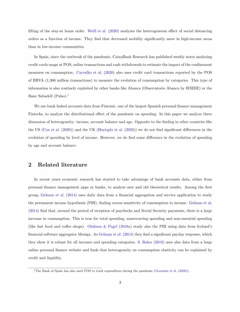
1 Introduction

The spread of COVID-19 has taken a huge toll on economic activity around the globe. Governments

have taken many actions to respond to the pandemic. However, there is a high degree of uncertainty

on the effect of the policy responses and the appropriateness of the total amount of public support to

the economy. Unfortunately, most of the official indicators and macroeconomic statistics have a very low

frequency, and are produced with long delays. This is an important challenge for policymakers in their efforts

to tailor their responses to “flatten the recession curve” Gourinchas (2020) after flattening the infection

curve. Our proposal is related with new international initiatives to track in real time (or with high frequency

indicators) the evolution of economic activity. For instance Cicala (2020) uses electricity usage from the

European grid to proxy the evolution of economic activity since the consumption of electricity is highly

correlated with its entrepreneurial usage. Bick & Blandin (2020) resort to the a Real Time Population

Survey (RPS), following the structure of the government survey (CPS) to construct high frequency estimates

of employment, hours worked and earnings. Chen et al. (2020) shows that these high-frequency measures of

energy consumption and hours worked are strongly correlated with the mobility indicators from the Google

Community Mobility Report. Chetty et al. (n.d.) have built an economic tracker to measure economic

activity at high-frequency in the US. They use anonymized economic information from private companies

to measure consumer spending (card-based transactions from Affinity Solutions); change in small business

open (business making transactions on a given day from Womply); time spent at work (GPS data provided

by Google); and hours worked at small business (provided by Homebase).

Researchers have already started to use high-frequency data to analyze the impact of economic stimulus

packages to mitigate the effect of the COVID-19 epidemic on economic activity. Two examples are the effect

on aggregate employment of the Paycheck Protection Program of the US Autor et al. (2020) or the effect on

consumption of the stimulus checks sent by the US Administration ? using data from financial aggregation

and service apps. Sheridan et al. (2020) use data from a large bank in Scandinavian to show that social

distancing laws had a small impact on economic activity. Sheridan et al. (2020) compares the data from

Sweden, which did not impose a strict confinement, with data from Denmark, that did close the economy.

The difference as a result of the shutdown are 4 additional percentage point of reduction in spending in

Denmark. This result agrees with the findings in Chetty et al. (n.d.) that show that the sharp reduction in

consumer spending, small business spending and time spent at work in the US economy started weeks before

the stay-at-home order and the non-essential business closure and did not recovered immediately after the

2

lifting of the stay-at home order. Weill et al. (2020) analyzes the heterogeneous effect of social distancing

orders as a function of income. They find that decreased mobility significantly more in high-income areas

than in low-income communities.

In Spain, since the outbreak of the pandemic, CaixaBank Research has published weekly notes analysing

credit cards usage at POS, online transactions and cash withdrawals to estimate the impact of the confinement

measures on consumption. Carvalho et al. (2020) also uses credit card transactions reported by the POS

of BBVA (1,300 million transactions) to measure the evolution of consumption by categories. This type of

information is also routinely exploited by other banks like Abanca (Observatorio Abanca by IESIDE) or the

Banc Sabadell (Pulso).1

We use bank linked accounts data from Fintonic, one of the largest Spanish personal finance management

Fintechs, to analyze the distributional effect of the pandemic on spending. In this paper we analyze three

dimension of heterogeneity: income, account balance and age. Opposite to the finding in other countries like

the US (Cox et al. (2020)) and the UK (Hacioglu et al. (2020)) we do not find significant differences in the

evolution of spending by level of income. However, we do find some difference in the evolution of spending

by age and account balance.

2 Related literature

In recent years economic research has started to take advantage of bank accounts data, either from

personal finance management apps or banks, to analyze new and old theoretical results. Among the first

group, Gelman et al. (2014) uses daily data from a financial aggregation and service application to study

the permanent income hypothesis (PIH), finding excess sensitivity of consumption to income. Gelman et al.

(2014) find that, around the period of reception of paychecks and Social Security payments, there is a large

increase in consumption. This is true for total spending, nonrecurring spending and non-essential spending

(like fast food and coffee shops). Olafsson & Pagel (2018a) study also the PIH using data from Iceland’s

financial software aggregator Meniga. As Gelman et al. (2014) they find a significant payday response, which

they show it is robust for all incomes and spending categories. S. Baker (2018) uses also data from a large

online personal finance website and finds that heterogeneity on consumption elasticity can be explained by

credit and liquidity.

1The Bank of Spain has also used POS to track expenditure during the pandemic (Gonzalez et al. (2020)).

3

But the analysis of the PIH is not the only theoretical result analyzed using data collected by online

financial services. Kuchler & Pagel (2020) shows that present-biased preferences can explain a large part

of the households’ inability to reduce debt and studies the differences between sophisticated and naive

consumers. Olafsson & Pagel (2018b) analyze the determinants of attention using the logins of users to their

accounts that do not generate a transaction as a proxy for attention. The empirical analysis is based on the

data of Meniga, a financial aggregation platform.

Research using bank account records is not limited to financial aggregation and service apps. Recently,

there has been an increasing interest in using data from large banks for empirical testing. Aspachs et al.

(2020) show how to calculate inequality at high frequency using the data of the second largest Spanish bank

(Caixabank). Cox et al. (2020) uses anonymized bank account information on several millions of JP Morgan

Chase customers to study the heterogeneous effect of the COVID-19 pandemic on spedning and savings.

Bank accounts data from online aggregation platforms or banks are very useful for economic research.

The enable a high-frequency analysis to capture changes in behavior or the effect of public policies, allowing

to fine tune them in the case of quickly spreading crisis as the COVID-19 pandemic. Bank accounts provide

also information that allows analizing the heterogeneity of the responds of individuals by demographic

characteristics and type of spending. Bank accounts data provide accurate and high-quality microdata that

do not suffer the recollection biases and measurement errors that plague survey-based data, especially when

asking for income data or requiring annotation of expenses by days. In addition, linked-account data, as the

one generated by personal management websites and apps, provide a more comprehensive view of the finances

of the users than accounts from a single bank. Obviously this advantage requires the selection of active users

that are ”well-linked” which is not an easy task. The raw data of financial aggregation platforms present

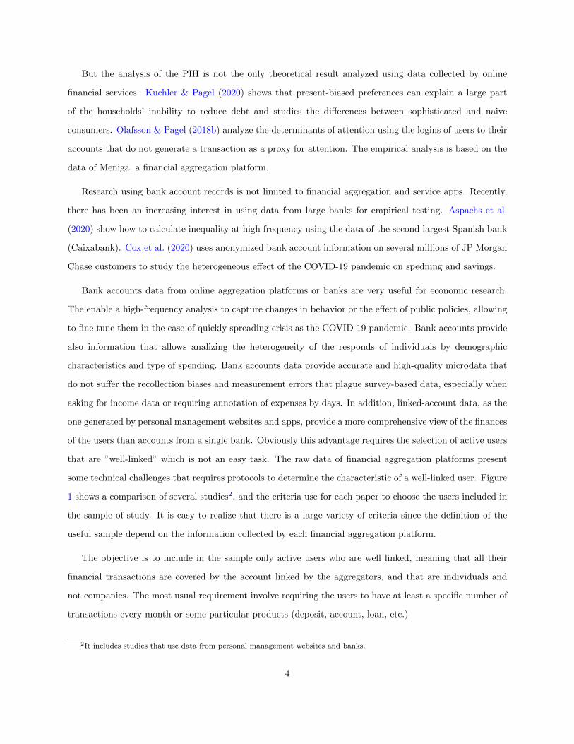
some technical challenges that requires protocols to determine the characteristic of a well-linked user. Figure

1 shows a comparison of several studies2, and the criteria use for each paper to choose the users included in

the sample of study. It is easy to realize that there is a large variety of criteria since the definition of the

useful sample depend on the information collected by each financial aggregation platform.

The objective is to include in the sample only active users who are well linked, meaning that all their

financial transactions are covered by the account linked by the aggregators, and that are individuals and

not companies. The most usual requirement involve requiring the users to have at least a specific number of

transactions every month or some particular products (deposit, account, loan, etc.)

2It includes studies that use data from personal management websites and banks.

4

(a) Personal finance management providers (PFM)

Hacioglu et al. (2020) Baker (2018) Gelman et al. (2014) Baker et al. (2020) Olafsson and Pagel (2018)Country UK US US US IcelandPFM Money Dashboard Large aggregator Check SaverLife Meniga (PFM)Transactions 4,386,200 7,400,000 52,731,354Users 8,365 156,606 23,000 5,746 66,262Dates 1‐Jan to 5‐Jul: 2019 and 2020 2008‐13 2012‐13 2011‐15Frequency Weekly Monthly Daily Daily DailyTransformation YoY Index Fraction of average daily spendingSample selection One current account 18 months of continuous data Different conditions for total spending, Users who update accounts until April 2020(active users) 200 pounds in debit Live in the US income, regular payment, liquidity and Several transactions per month in 2020

minimum of 5 transactions month Log into account in the past 6 months well‐linked observations Transacted at least $1000 during three months(Jan19‐June20) Enter age, sex, location, income, marital status

Refreshed accounts in July 2020 At least three linked accountLess than 11 active accounts Fewer than 25% uncategorized dataMonthly debit less than 100K Linked to publicly traded firm as an employer

Monthly total expenditure > 100 in all months minus oneWorking age population

Exclude after tax income in 2019 above 2019

(a) Personal finance management providers (cont.) (b) Banks and other financial instiuttions

Kuchler et al. (2018) Olafsson et al. (2018) Sheridan et al. (2020) Aspachs et al. (2020) Cox et al. (2020)Country US Iceland Denmark / Sweden Spain USBank / PFM ReadyForZero Meniga Danske Bank Caixabank JP Morgan ChaseTransactions 520,000,000Users 516 52,545 860,000 3,028,204 5,014,672Dates Sept‐2009: Sept‐2012 2011‐2017 Jan‐2018: Apr‐20 2019‐20Frequency Daily Daily Daily Monthly WeeklyTransformation Level YoY over average 2019 YoY over 2019 YoYSample selection Exclude users who linked more account later in the sample Users for which account balances or credit(active users) Bi‐weekly payments lines are observed Minimum one card payment per month Only one account holder or one employer Minimum 5 checking account transactions

Regular paychecks more than 70% of all income Observed income arrivals (Jan18‐dec‐19) paying‐in wages and 3 card transactions every monthObserved at least 180 days after sign‐up Key demographic information available Observed wage or government benefits during (Jan18‐March20)

at least 8 regular, non‐constrained pay cycles (age, sex, postal code) two months (December of 2019 and January labor income 12000 dollars in 2018 and 2019 at least 45 days of positive spending 5 food transactions in at least 23 months of 2020)

of a 24 months period Individuals between 16 and 64 years old

Figure 1: Selected studies using bank account information

3 Data

Our data on financial transactions are collected by Fintonic, the first Spanish personal finance app, in

the course of its regular business. Users can link all their financial accounts to the app, that logs into a web

portals of financial institutions where they obtain the primary data. The main advantage of data from an

account information service provider (AISP), popularly known as ”financial aggregators”, is the fact that it

allows users to have a 360 degrees view of the finances of the individuals. This comprehensive view of the

financial situation of the user is one of the most attractive characteristics of the financial aggregators. The

resulting income and expenditure data are comprehensive given that they are capture from several financial

sources that are linked by Fintonic. The initial sample included 236,053 single users3. The raw data includes

around 250 million transactions on de-identified users covering the period from January 1, 2019 until June

3We eliminated 4 observations that were duplicated in the original sample.

5

30, 2020.4

To get an accurate picture of the finances of the individuals in the sample from the raw data there are

some conceptual and technical challenges. The objective is to capture data from users that are reasonably

well-linked and avoid clients who may use Fintonic for business-related purposes. The large majority of the

user of personal finance websites are individuals but there is always the possibility that a company may also

use the aggregator, although in their case it is not so useful since they should keep accounting books. They

have always an updated view of their financial situation and, therefore, less incentives to use the advantages

of the aggregator. Therefore, in order to get an accurate and comprehensive view of the users, we impose

some conditions on the individuals who are included in the sample. First of all, they should have accessed at

least once to their Fintonic account during the last 45 days before the last day of the sample, June 30, 2020.

Second, we exclude users that have more than 7 active accounts, which is quite improbable for a non-business

user. Third, we consider only the users that have at least five transactions related with expenditures per

month. We created weekly and daily measures of aggregate expenditure by adding up electronic spending

(credit and debit card charges) and cash (ATM and window cash withdrawals).5 This criterion is common

to other research using similar data and guarantees a certain stability in the sample. Finally, we impose

limits on the size of each transaction. We eliminate the transactions with a value above the sum of the

mean expenditure in that category plus five standard deviations6.Considering this conditions the sample is

reduced to 163,292 active, well-linked users.

One preliminary check is the user base representativeness. Since our main source of data is related with

holding a bank account it is important to start analyzing the level of financial inclusion in Spain. The data

of the Global Findex, the index of financial inclusion of the World Bank, shows that 97.6% of Spanish people

over 15 years old holds a banking account when the average in high-income countries is 93.7%.

We know from the general profile of users of online services, and previous research, that user of the

services of financial aggregation are with high probability male and urban. Users are also younger and richer

than the general population. The data of Fintonic are not an exception to this profile. Men are 65.8% of

the users while, in the general population at the beginning of 2020 they represented less than 50% of the

4The data were treated with a differential privacy algorithm before researchers have access to them.5We do not count recurring bills as transactions considered as expenditure. Therefore, a user may have five recurring bills

and not being included in the sample. We do not consider paper checks since in the Spanish case these are very rare. We alsoeliminate those users that, on average, complete more than 100 transactions per month.

6Results are very similar if we eliminate users that have an average expenditure of more than 3000 euros per month.

6

population above 18 years old (48.6%)7. Something similar happens with age. A high proportion of the

user of Fintonic, 78.4%, are less than 45 years old while in the population between 18 and 44 years old was

41.2%. This type of age imbalance is also typical of data from online personal management aggregators.

The solution to this situation is to reweight the sample using the official population statistics.

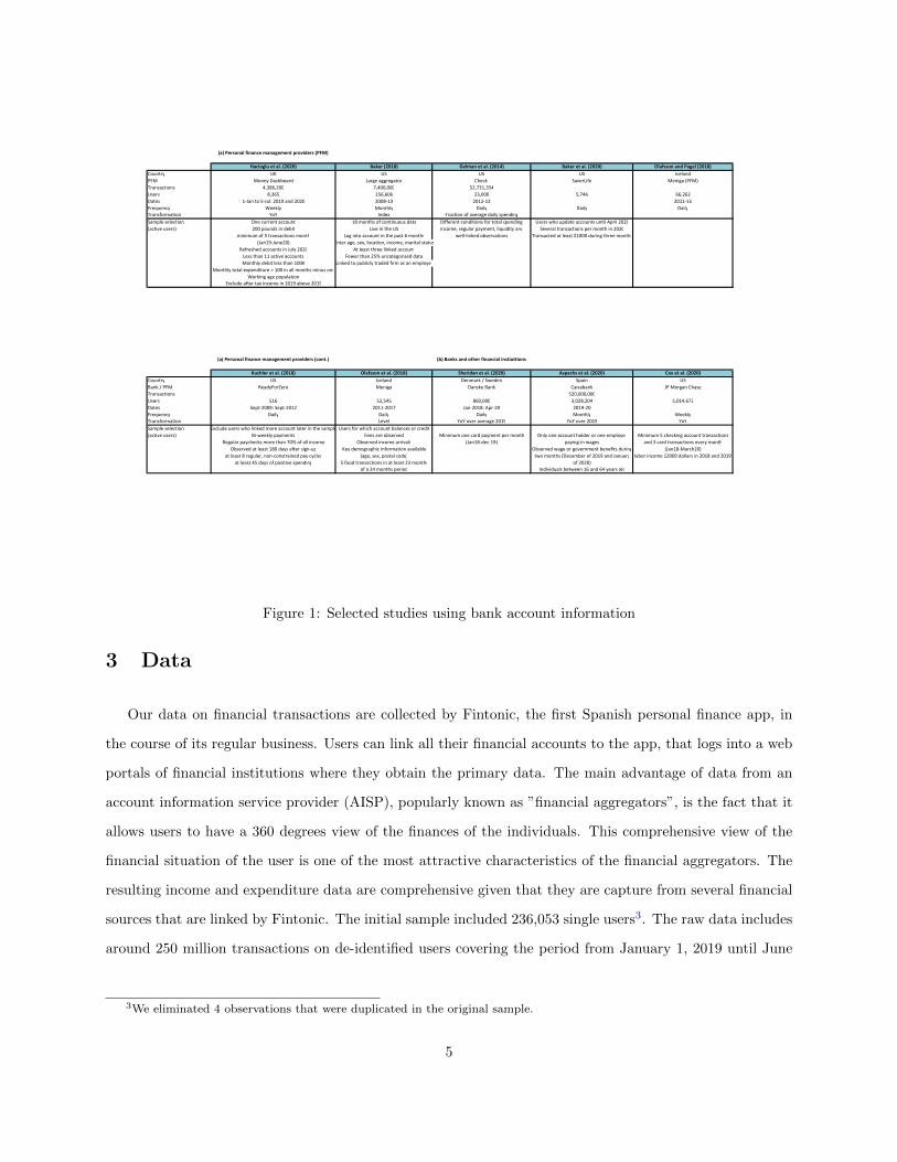
4 The evolution of expenditure

We first look at the evolution of expenditure. In this category we do not include recurring bills (electricity,

phone, rental, etc.). Figure 2 shows that the evolution of the growth rate of monthly expenditure is more

variable than the total of expenditure plus recurring bills. Obviously recurring bills, especially the ones

related with housing services, cannot be adjusted as much as many other expenditures.

-50%

-40%

-30%

-20%

-10%

0%

10%

20%

jan20 feb-20 mar-20 apr20 may-20 jun-20

Expenditure Expenditure + recurring bills

Figure 2: Expenditure versus Total consumption

In order to calculate the weekly change in expenditure between the same weeks of different years we need

to deal with seasonal effects. In particular, some weeks may have different number of holidays and working

days. There are also moving holidays that can affect the temporal shape of expenditures in two consecutive

years. For instance, Eastern happens in the 15th week in 2019 and in week 16th in 2020. To eliminate the

7All the ratios refer to the population of people above 18 years old. Notice that being this percentage almost 17 percentagepoint above the population it is closer than the proportion of male in other samples. For instance in S. R. Baker et al. (2020)the proportion of males reaches the 85% while in Gelman et al. (2014) is 59.93%.

7

effect of moving holidays in the weekly data we run the regression,

yt = α+ β0NHt + β1WDt + δPOSTt + γ0NHt ∗ POSTt + γ1WDt ∗ POSTt + ut (1)

where y is expenditure; NH is the number of holidays in the week; WD are working days in the week; POST

is a dummy variable that takes value 1 if t is in the shutdown period. The adjusted value is

yt = yt − β0NHt + β1WDt + γ0NHt ∗ POSTt + γ1WDt ∗ POSTt (2)

Once the transformation has eliminated the effect of moving holidays, we deal with seasonality calculating

the growth rate of each week versus the same week of the previous year.8

∆yt =(yt − yt−52)

yt−52(3)

The are alternative approaches to deal with the seasonality. For instance we could calculate the difference

between two weeks one year apart over the average of expenditure of year 2019.9

∆yt =(yt − yt−52)

y2019(4)

In our case the application of this transformation produces almost the same results as the weekly growth

rate using the corresponding week of the previous year as the base.

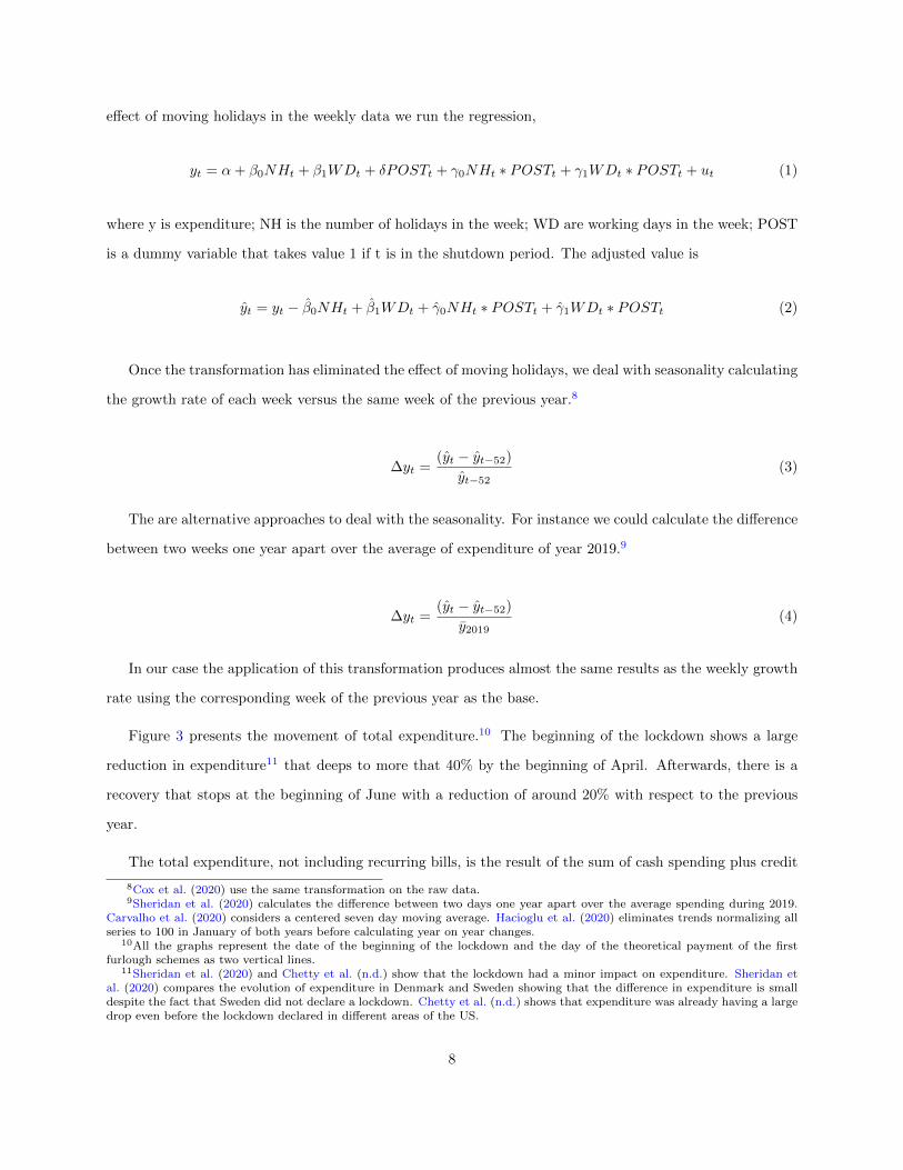
Figure 3 presents the movement of total expenditure.10 The beginning of the lockdown shows a large

reduction in expenditure11 that deeps to more that 40% by the beginning of April. Afterwards, there is a

recovery that stops at the beginning of June with a reduction of around 20% with respect to the previous

year.

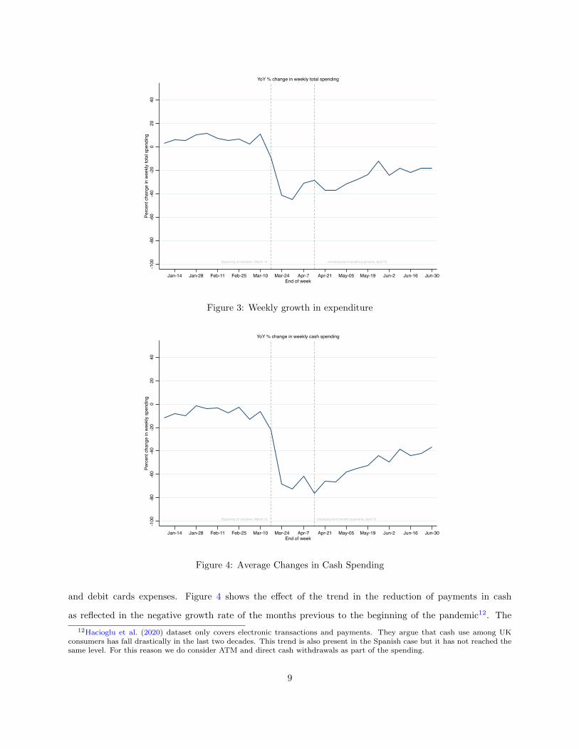
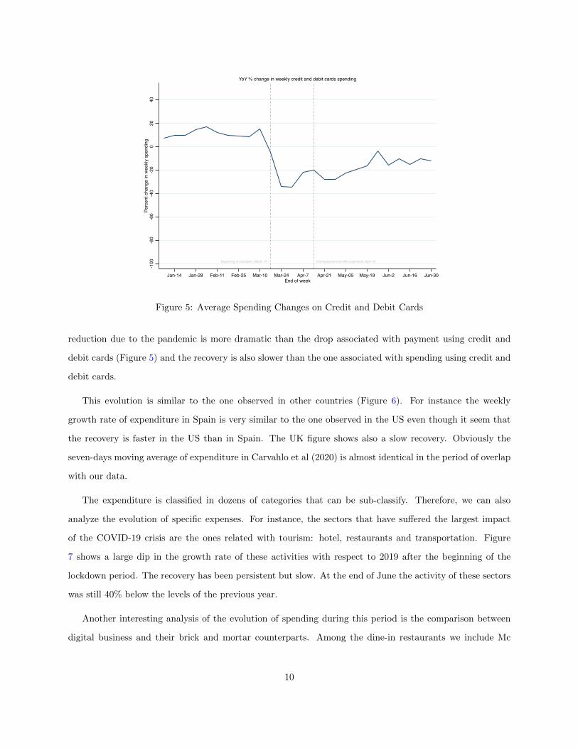
The total expenditure, not including recurring bills, is the result of the sum of cash spending plus credit

8Cox et al. (2020) use the same transformation on the raw data.9Sheridan et al. (2020) calculates the difference between two days one year apart over the average spending during 2019.

Carvalho et al. (2020) considers a centered seven day moving average. Hacioglu et al. (2020) eliminates trends normalizing allseries to 100 in January of both years before calculating year on year changes.

10All the graphs represent the date of the beginning of the lockdown and the day of the theoretical payment of the firstfurlough schemes as two vertical lines.

11Sheridan et al. (2020) and Chetty et al. (n.d.) show that the lockdown had a minor impact on expenditure. Sheridan etal. (2020) compares the evolution of expenditure in Denmark and Sweden showing that the difference in expenditure is smalldespite the fact that Sweden did not declare a lockdown. Chetty et al. (n.d.) shows that expenditure was already having a largedrop even before the lockdown declared in different areas of the US.

8

Beginning of lockdown, March 14 Unemployment benefits payments, April 10

-100

-80

-60

-40

-20

020

40Pe

rcen

t cha

nge

in w

eekl

y to

tal s

pend

ing

Jan-14 Jan-28 Feb-11 Feb-25 Mar-10 Mar-24 Apr-7 Apr-21 May-05 May-19 Jun-2 Jun-16 Jun-30End of week

YoY % change in weekly total spending

Figure 3: Weekly growth in expenditure


-100

-80

-60

-40

-20

020

40Pe

rcen

t cha

nge

in w

eekl

y sp

endi

ng


YoY % change in weekly cash spending

Figure 4: Average Changes in Cash Spending

and debit cards expenses. Figure 4 shows the effect of the trend in the reduction of payments in cash

as reflected in the negative growth rate of the months previous to the beginning of the pandemic12. The

12Hacioglu et al. (2020) dataset only covers electronic transactions and payments. They argue that cash use among UKconsumers has fall drastically in the last two decades. This trend is also present in the Spanish case but it has not reached thesame level. For this reason we do consider ATM and direct cash withdrawals as part of the spending.

9


-100

-80

-60

-40

-20

020

40Pe

rcen

t cha

nge

in w

eekl

y sp

endi

ng


YoY % change in weekly credit and debit cards spending

Figure 5: Average Spending Changes on Credit and Debit Cards

reduction due to the pandemic is more dramatic than the drop associated with payment using credit and

debit cards (Figure 5) and the recovery is also slower than the one associated with spending using credit and

debit cards.

This evolution is similar to the one observed in other countries (Figure 6). For instance the weekly

growth rate of expenditure in Spain is very similar to the one observed in the US even though it seem that

the recovery is faster in the US than in Spain. The UK figure shows also a slow recovery. Obviously the

seven-days moving average of expenditure in Carvahlo et al (2020) is almost identical in the period of overlap

with our data.

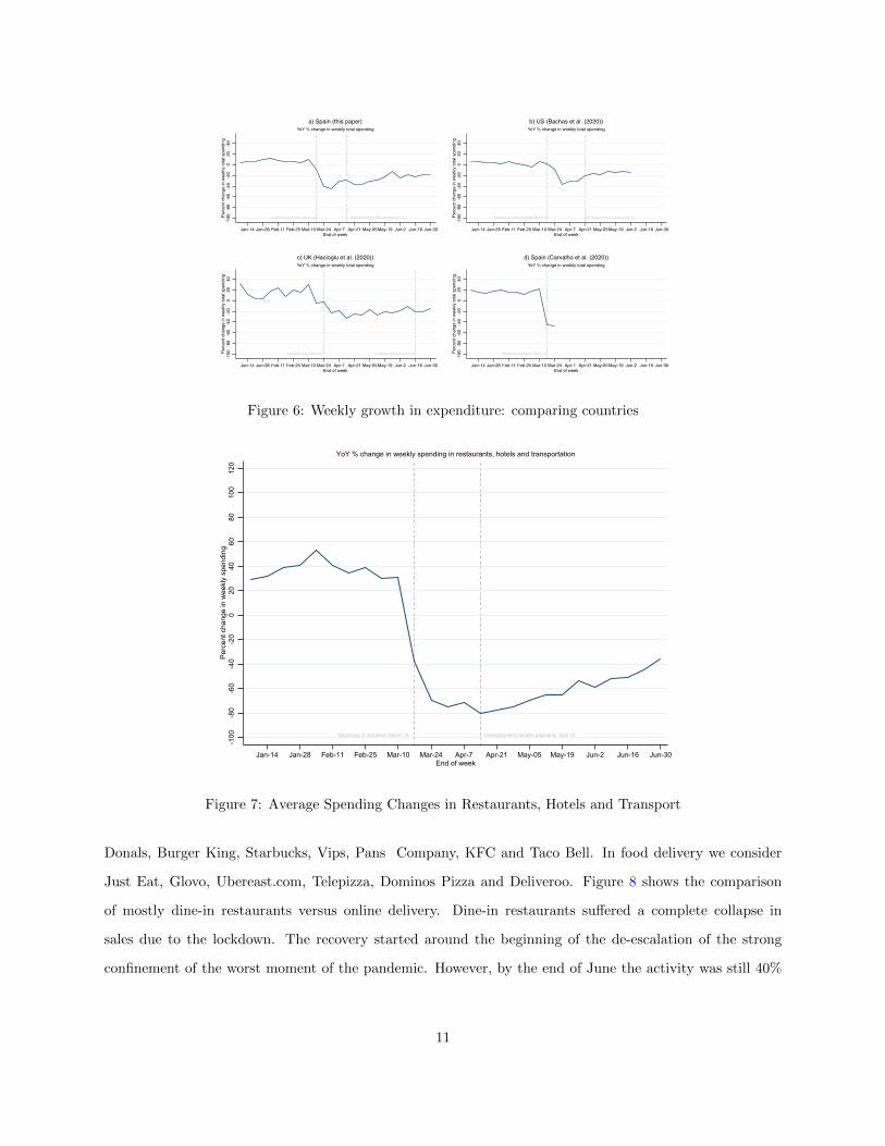
The expenditure is classified in dozens of categories that can be sub-classify. Therefore, we can also

analyze the evolution of specific expenses. For instance, the sectors that have suffered the largest impact

of the COVID-19 crisis are the ones related with tourism: hotel, restaurants and transportation. Figure

7 shows a large dip in the growth rate of these activities with respect to 2019 after the beginning of the

lockdown period. The recovery has been persistent but slow. At the end of June the activity of these sectors

was still 40% below the levels of the previous year.

Another interesting analysis of the evolution of spending during this period is the comparison between

digital business and their brick and mortar counterparts. Among the dine-in restaurants we include Mc

10


-100

-80

-60

-40

-20

020

40Pe

rcen

t cha

nge

in w

eekl

y to

tal s

pend

ing

Jan-14 Jan-28 Feb-11 Feb-25 Mar-10 Mar-24 Apr-7 Apr-21 May-05May-19 Jun-2 Jun-16 Jun-30End of week

YoY % change in weekly total spendinga) Spain (this paper)

National emergency declared, March 13 EIP payments from Treasury, April 15

-100

-80

-60

-40

-20

020

40Pe

rcen

t cha

nge

in w

eekl

y to

tal s

pend

ing


YoY % change in weekly total spendingb) US (Bachas et al. (2020))

Lockdown start, March 23 Lockdown relaxation, June 15

-100

-80

-60

-40

-20

020

40Pe

rcen

t cha

nge

in w

eekl

y to

tal s

pend

ing


YoY % change in weekly total spendingc) UK (Hacioglu et al. (2020))

Beginning of lockdown, March 14

-100

-80

-60

-40

-20

020

40Pe

rcen

t cha

nge

in w

eekl

y to

tal s

pend

ing


YoY % change in weekly total spendingd) Spain (Carvalho et al. (2020))

Figure 6: Weekly growth in expenditure: comparing countries


-100

-80

-60

-40

-20

020

4060

8010

012

0Pe

rcen

t cha

nge

in w

eekl

y sp

endi

ng


YoY % change in weekly spending in restaurants, hotels and transportation

Figure 7: Average Spending Changes in Restaurants, Hotels and Transport

Donals, Burger King, Starbucks, Vips, Pans Company, KFC and Taco Bell. In food delivery we consider

Just Eat, Glovo, Ubereast.com, Telepizza, Dominos Pizza and Deliveroo. Figure 8 shows the comparison

of mostly dine-in restaurants versus online delivery. Dine-in restaurants suffered a complete collapse in

sales due to the lockdown. The recovery started around the beginning of the de-escalation of the strong

confinement of the worst moment of the pandemic. However, by the end of June the activity was still 40%

11

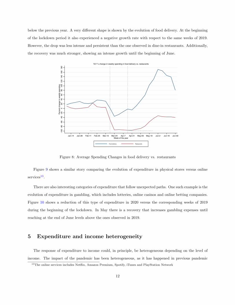
below the previous year. A very different shape is shown by the evolution of food delivery. At the beginning

of the lockdown period it also experienced a negative growth rate with respect to the same weeks of 2019.

However, the drop was less intense and persistent than the one observed in dine-in restaurants. Additionally,

the recovery was much stronger, showing an intense growth until the beginning of June.


-100

-80

-60

-40

-20

020

4060

8010

012

014

016

018

0Pe

rcen

t cha

nge

in w

eekl

y sp

endi

ng

Jan-14 Jan-28 Feb-11 Feb-25 Mar-10 Mar-24 Apr-7 Apr-21 May-05 May-19 Jun-2 Jun-16 Jun-30Week of the year

Food delivery Restaurants

YoY % change in weekly spending in food delivery vs. restaurants

Figure 8: Average Spending Changes in food delivery vs. restaurants

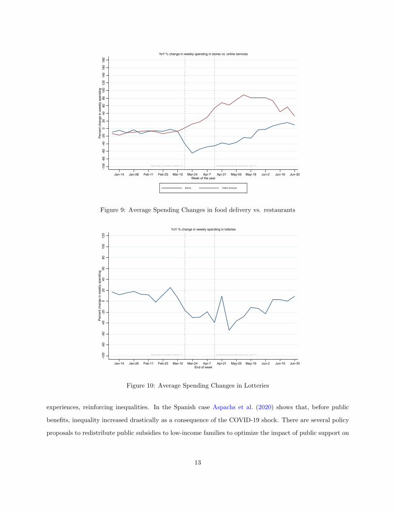
Figure 9 shows a similar story comparing the evolution of expenditure in physical stores versus online

services13.

There are also interesting categories of expenditure that follow unexpected paths. One such example is the

evolution of expenditure in gambling, which includes lotteries, online casinos and online betting companies.

Figure 10 shows a reduction of this type of expenditure in 2020 versus the corresponding weeks of 2019

during the beginning of the lockdown. In May there is a recovery that increases gambling expenses until

reaching at the end of June levels above the ones observed in 2019.

5 Expenditure and income heterogeneity

The response of expenditure to income could, in principle, be heterogeneous depending on the level of

income. The impact of the pandemic has been heterogeneous, as it has happened in previous pandemic

13The online services includes Netflix, Amazon Premium, Spotify, iTunes and PlayStation Network

12


-100

-80

-60

-40

-20

020

4060

8010

012

014

016

018

0Pe

rcen

t cha

nge

in w

eekly

spe

ndin

g


Stores Online services

YoY % change in weekly spending in stores vs. online services

Figure 9: Average Spending Changes in food delivery vs. restaurants


-100

-80

-60

-40

-20

020

4060

8010

012

0Pe

rcen

t cha

nge

in w

eekl

y sp

endi

ng


YoY % change in weekly spending in lotteries

Figure 10: Average Spending Changes in Lotteries

experiences, reinforcing inequalities. In the Spanish case Aspachs et al. (2020) shows that, before public

benefits, inequality increased drastically as a consequence of the COVID-19 shock. There are several policy

proposals to redistribute public subsidies to low-income families to optimize the impact of public support on

13

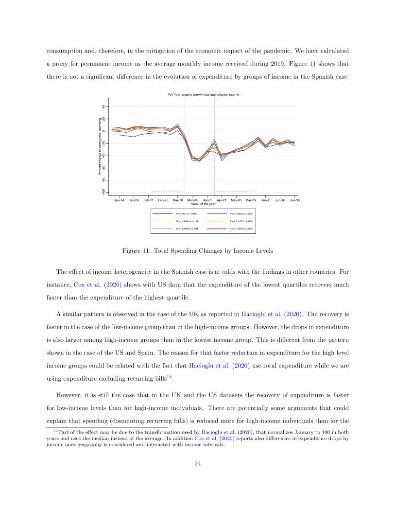
consumption and, therefore, in the mitigation of the economic impact of the pandemic. We have calculated

a proxy for permanent income as the average monthly income received during 2019. Figure 11 shows that

there is not a significant difference in the evolution of expenditure by groups of income in the Spanish case.


-100

-80

-60

-40

-20

020

40Pe

rcen

t cha

nge

in w

eekl

y to

tal s

pend

ing


From 584€ to 1,083€ From 1,084€ to 1,583€

From 1,584€ to 2,416€ From 2,417€ to 3,333€

From 3,334€ to 4,166€ From 4,167€ to 5,000€

YoY % change in weekly total spending by income

Figure 11: Total Spending Changes by Income Levels

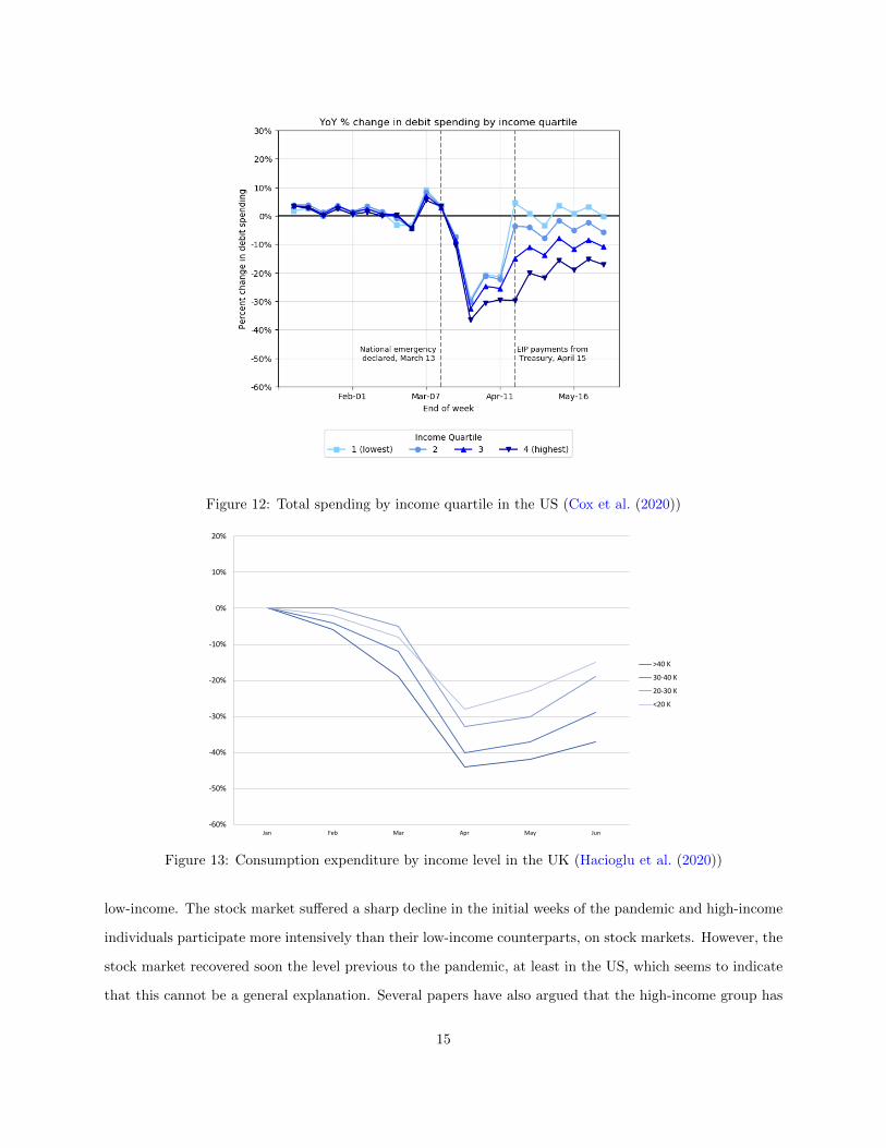
The effect of income heterogeneity in the Spanish case is at odds with the findings in other countries. For

instance, Cox et al. (2020) shows with US data that the expenditure of the lowest quartiles recovers much

faster than the expenditure of the highest quartile.

A similar pattern is observed in the case of the UK as reported in Hacioglu et al. (2020). The recovery is

faster in the case of the low-income group than in the high-income groups. However, the drops in expenditure

is also larger among high-income groups than in the lowest income group. This is different from the pattern

shown in the case of the US and Spain. The reason for that faster reduction in expenditure for the high level

income groups could be related with the fact that Hacioglu et al. (2020) use total expenditure while we are

using expenditure excluding recurring bills14.

However, it is still the case that in the UK and the US datasets the recovery of expenditure is faster

for low-income levels than for high-income individuals. There are potentially some arguments that could

explain that spending (discounting recurring bills) is reduced more for high-income individuals than for the

14Part of the effect may be due to the transformation used by Hacioglu et al. (2020), that normalizes January to 100 in bothyears and uses the median instead of the average. In addition Cox et al. (2020) reports also differences in expenditure drops byincome once geography is considered and interacted with income intervals.

14

Result 1: Spending recovers faster for low incomehouseholds

Large and pervasive initial declines. Credit card spend

Faster recovery in spending for lower income households.

Similar patterns in lower-income sectors. Details

5 / 12

Figure 12: Total spending by income quartile in the US (Cox et al. (2020))

-60%

-50%

-40%

-30%

-20%

-10%

0%

10%

20%

Jan Feb Mar Apr May Jun

>40 K

30-40 K

20-30 K

<20 K

Figure 13: Consumption expenditure by income level in the UK (Hacioglu et al. (2020))

low-income. The stock market suffered a sharp decline in the initial weeks of the pandemic and high-income

individuals participate more intensively than their low-income counterparts, on stock markets. However, the

stock market recovered soon the level previous to the pandemic, at least in the US, which seems to indicate

that this cannot be a general explanation. Several papers have also argued that the high-income group has

15

a larger share of non-essential expenditures than the low-income households.15 However, the most likely

explanation is the increase in government assistance centered around low-income households. In the US case

this explanation is very likely since the tax rebates received by low-income households added to the extended

UI derived from the Federal Pandemic Unemployment Compensation, which implied a wage replacement over

100 percent for many low-income workers who lost their jobs. In the case of the UK this explanation is less

likely despite the fact that low-income household received a much larger amount of government benefits than

high-income households. In the Spanish case even though government benefits, especially furlough schemes,

have supported the income of temporary layoff workers, the replacement rate was less than 100 percent. In

addition the Spanish stock market did not recovered the pre-pandemic level, being still 25% below in June.

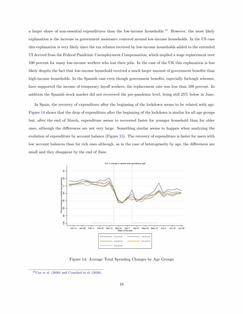
In Spain, the recovery of expenditure after the beginning of the lockdown seems to be related with age.

Figure 14 shows that the drop of expenditure after the beginning of the lockdown is similar for all age groups

but, after the end of March, expenditure seems to recovered faster for younger household than for older

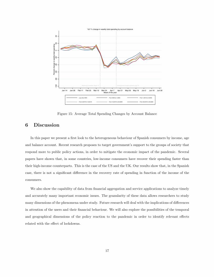
ones, although the differences are not very large. Something similar seems to happen when analyzing the

evolution of expenditure by account balance (Figure 15). The recovery of expenditure is faster for users with

low account balances than for rich ones although, as in the case of heterogeneity by age, the differences are

small and they disappear by the end of June.


-100

-80

-60

-40

-20

020

40Pe

rcen

t cha

nge

in w

eekl

y to

tal s

pend

ing


From 18 to 24 From 25 to 34

From 35 to 44 From 45 to 54

From 55 to 64

YoY % change in weekly total spending by age

Figure 14: Average Total Spending Changes by Age Groups

15Cox et al. (2020) and Crawford et al. (2020).

16


-100

-80

-60

-40

-20

020

40Pe

rcen

t cha

nge

in w

eekl

y to

tal s

pend

ing


Less than 250€ From 250€ to 1,000€ From 1,001€ to 5,000€

From 5,001€ to 10,001€ From 10,001€ to 20,000€ From 20,001€ to 40,000€

YoY % change in weekly total spending by account balance

Figure 15: Average Total Spending Changes by Account Balance

6 Discussion

In this paper we present a first look to the heterogeneous behaviour of Spanish consumers by income, age

and balance account. Recent research proposes to target government’s support to the groups of society that

respond more to public policy actions, in order to mitigate the economic impact of the pandemic. Several

papers have shown that, in some countries, low-income consumers have recover their spending faster than

their high-income counterparts. This is the case of the US and the UK. Our results show that, in the Spanish

case, there is not a significant difference in the recovery rate of spending in function of the income of the

consumers.

We also show the capability of data from financial aggregation and service applications to analyze timely

and accurately many important economic issues. The granularity of these data allows researchers to study

many dimensions of the phenomena under study. Future research will deal with the implications of differences

in attention of the users and their financial behaviour. We will also explore the possibilities of the temporal

and geographical dimensions of the policy reaction to the pandemic in order to identify relevant effects

related with the effect of lockdowns.

17

References

Aspachs, O., Durante, R., Graziano, A., Mestres, J., Montalvo, J., & Reynal-Querol, M. (2020). Real-time

inequality and the welfare state in motion: evidence from covid-19 in spain. CEPR Discussion Paper

15118 .

Autor, D., Cho, D., Crane, L., Goldar, M., Lutz, B., Montes, J., . . . Yildirmaz, A. (2020). An evaluation of

the paycheck protection program using administrative payroll microdata. MIT Working Paper .

Baker, S. (2018). Debt and the response of household income to shocks: validation and application of linked

financial account data. Journal of Political Economy , 126 (4), 1504-1556.

Baker, S. R., Farrokhnia, R. A., Meyer, S., Pagel, M., & Yannelis, C. (2020). Income, liquidity, and

the consumption response to the 2020 economic stimulus payments. Review of Asset Pricing Studies,

Forthcoming.

Bick, A., & Blandin, A. (2020). Real time labor market estimates during the 2020 coronavirus outbreak.

Unpublished Manuscript, Arizona State University .

Carvalho, V. M., Hansen, S., Ortiz, A., Garcia, J. R., Rodrigo, T., Rodriguez Mora, S., & Ruiz de Aguirre,

P. (2020). Tracking the covid-19 crisis with high-resolution transaction data. , CEPR Discussion Paper

No. DP14642 .

Chen, S., Igan, D., Pierri, N., & Presbitero, A. F. (2020). Tracking the economic impact of covid-19 and

mitigation policies in europe and the united states. IMF WP/20/125 .

Chetty, R., Friedman, J. N., Hendren, N., & Stepner, M. (n.d.). Real-time economics: A new platform to

track the impacts of covid-19 on people, businesses, and communities using private sector data. , NBER

Working Paper 27,431 .

Cicala, S. (2020). Early economic impacts of covid-19 in europe: A view from the grid. unpublished

manuscript.

Cox, N., Ganong, P., Noel, P., Vara, J., Wong, A., Farrell, D., & Greig, F. (2020). Initial impact of the

pandemic on consumer behavior: evidence from linked income, spending, and savings data. Brookings

Papers on Economic Activity , Forthcoming.

18

Crawford, R., Davenport, J., Joyce, R., & Levell, P. (2020). Household spending and coronavirus. Institute

of Fiscal Studies, Note 14,795 .

Gelman, M., Kariv, S., Shapiro, M. D., Silverman, D., & Tadelis, S. (2014). Harnessing naturally occurring

data to measure the response of spending to income. Science, 345 (6193), 212–215.

Gonzalez, J., Urtasum, A., & Perez, M. (2020). Evolucion del consumo en espana durante la vigencia del

estado de alarma: un analisis a paritr del gasto con tarjetas de pago. Articulos Analiticos, 3/2020 .

Gourinchas, P.-O. (2020). Flattening the pandemic and recession curves. Mitigating the COVID Economic

Crisis: Act Fast and Do Whatever , 31.

Hacioglu, S., Kanzig, D., & Surico, P. (2020). The distributional impact of the pandemic. CEPR Discussion

Paper 15101 .

Kuchler, T., & Pagel, M. (2020). Sticking to your plan: the role of present bias for credit card paydown.

Journal of Financial Economics, Forthcoming.

Olafsson, A., & Pagel, M. (2018a). The liquid hand-to-mouth: evidence from personal finance management

software. Review of Financial Economics, 31 (11), 4398-4446.

Olafsson, A., & Pagel, M. (2018b). The ostrich in us: Selective attention to personal finance. mimeo.

Sheridan, A., Andersen, A., Hansen, E., & Johannesen, N. (2020). Social distancing laws cause only

small losses of economic activity during the covid-19 pandemic in scandinavia. Proceeding of the National

Academy of Sciences(August 2020), 1-6.

Weill, J., Stigler, M., Deschenes, O., & Springborn, M. (2020). Social distancing responses to covid-19 emer-

gency declaration strongly differentiated by income. Proceeding of the National Academy of Sciences(July

2020), 1-3.

19

Distributional effects of COVID-19 on spending: A first ...

Documents

Transcript of Distributional effects of COVID-19 on spending: A first ...