Proceedings of Informing Science & IT Education Conference (InSITE) 2015 Cite as: McMaster, K., Sambasivam, S., Rague, B., & Wolthuis, S. (2015). Distribution of Execution Times for Sorting Algorithms Implemented in Java. Proceedings of Informing Science & IT Education Conference (InSITE) 2015, 269-283. Retrieved from http://Proceedings.InformingScience.org/InSITE2015/InSITE15p269-283McMaster1516.pdf

Editor: Eli Cohen

Distribution of Execution Times for Sorting Algorithms Implemented in Java

Kirby McMaster Moravian College,

Bethlehem, PA, USA kmcmaster@weber.edu

Samuel Sambasivam Azusa Pacific University,

Azusa, CA, USA ssambasivam@apu.edu

Brian Rague Weber State University,

Ogden, UT, USA brague@weber.edu

Stuart Wolthuis Brigham Young University-

Hawaii, Laie, HI, USA stuartlw@byuh.edu

Abstract Algorithm performance coverage in textbooks emphasizes patterns of growth in execution times, relative to the size of the problem. Variability in execution times for a given problem size is usu-ally ignored. In this research study, our primary focus is on the empirical distribution of execution times for a given algorithm and problem size. We examine CPU times for Java implementations of five sorting algorithms for arrays: selection sort, insertion sort, shell sort, merge sort, and quicksort. We measure variation in running times for these algorithms and describe how the sort-time distributions change as the problem size increases. Using our research methodology, we compare the relative stability of performance for the different sorting algorithms.

Keywords: algorithm, sorting, performance, distribution, variation, Java.

Introduction Courses in data structures and algorithms are the meat and potatoes of Computer Science pro-grams. Data Structures textbooks (Kaufman & Wolfgang, 2010; Lafore, 2003; Main & Savich, 2010) emphasize how to implement algorithms to support complex data structures such as stacks, queues, search trees, and graphs. Different algorithms are required when arrays vs. linked lists are used to represent data structures. An introduction to order-of-growth concepts relates problem

size to execution time for various algo-rithms.

In Analysis of Algorithms textbooks (Cormen, et al., 2009; Kleinberg & Tar-dos, 2006; Aho, Ullman & Hopcroft, 1983), explanations of algorithm per-formance place greater emphasis on mathematical reasoning. This is also true of the early Algorithms books by Aho (1974) and Knuth (1998).

Material published as part of this publication, either on-line or in print, is copyrighted by the Informing Science Institute. Permission to make digital or paper copy of part or all of these works for personal or classroom use is granted without fee provided that the copies are not made or distributed for profit or commercial advantage AND that copies 1) bear this notice in full and 2) give the full citation on the first page. It is per-missible to abstract these works so long as credit is given. To copy in all other cases or to republish or to post on a server or to redistribute to lists requires specific permission and payment of a fee. Contact Publisher@InformingScience.org to request redistribution permission.

Execution Times for Sorting Algorithms

270

A formal examination of algorithm efficiency based on resources required (primarily CPU time) looks at best-case, worst-case, and average-case situations. Much of the discussion centers on worst-case analysis because the mathematical arguments are simpler, and the results have more pedagogical and practical relevance. Order-of-growth is simplified by ignoring constants and lower order terms, so average-case results are often proportional to the worst-case. The study of variation is mostly restricted to comparisons of best-case and worst-case results with average-case.

Sedgewick & Wayne (2011) present a mathematical analysis of algorithms, and then briefly relate their mathematical models to empirical results. They give several algorithms for finding three numbers that sum to zero (from a large input file). They ran each algorithm once for each input file, assuming that the only source of variation would be the actual data. In some of our tests, we experienced situations where repeated execution of the same algorithm on the same (non-randomized) data resulted in different execution times, indicating the existence of other sources of variation.

Algorithm analysis in some textbooks briefly mentions that running times can vary for different inputs, but the books include little discussion of the distribution of execution times for repeated tests. Variation includes not only dispersion (how spread out the scores are from a central value), but also skewness (how unbalanced the scores are at each end of the distribution).

It is difficult to find individual research efforts on sorting algorithms that focus on variation. An interesting study by Musselman (2007) examined robustness as a measure of algorithm perfor-mance. An earlier study (Helman, Bader & JaJa, 1998) performed an experiment on a randomized parallel sorting algorithm.

Variation can be more important than averages or even generalized worst-case analysis when consistency and dependability of execution time is a requirement. This is common in systems having strict time constraints on operations, such as manufacturing systems, real-time control sys-tems, and embedded systems.

Sources of Variation There are many system features which can affect algorithm performance. In this research, we use CPU time as our primary measure of performance. A layered list of sources of variation is out-lined below.

1. Computer hardware components: (a) CPU clock speed, pipelines, number of cores, internal caches, and (b) memory architecture, amount of RAM, external caches.

2. Operating system features: (a) process scheduling algorithms, multi-tasking, parallel process ing, and (b) memory allocation algorithms, virtual memory.

3. For Java programs: (a) JIT compiler optimizations, (b) run-time options and behavior, and (c) memory management, including automatic garbage collection (Goetz, 2004; Boyer, 2008; Wicht, 2011).

4. Application program: (a) choice of algorithm, and how it is implemented, (b) size of problem, (c) amount of memory required by the algorithm, and (d) data type, data source, and data structure.

Research Plan The primary objective of this research is to examine how algorithm execution time distributions depend on problem size, randomness of data, and other factors. We limit our attention to sorting algorithms for arrays, including selection sort, insertion sort, shell sort, merge sort and quicksort.

McMaster, Sambasivam, Rague, & Wolthuis

271

For a range of array sizes, we ran a Java program that repeatedly filled an array with random in-tegers, sorted the data using one of the sorting algorithms, and measured the elapsed time. The program then output summary statistics to describe the distribution of sort-times.

To isolate algorithm performance variation from the hardware, operating system, and Java layers, we ran all final results on a single computer. This computer had an Intel Core2 Duo CPU, Win-dows 7 operating system, and Version 7 of the Java compiler and run-time.

In our research environment, we assumed that algorithm execution times would depend almost entirely on:

1. the sorting algorithm

2. the size and data type of the array

3. the randomness of the generated data

However, this assumption was not supported by our tests. Unexpected sources of variation in ex-ecution times were encountered throughout our research study. These surprising patterns required procedures for generating and analyzing performance data that are relatively immune to outlier effects.

In the next section, we carefully examine a typical sort-time distribution that guided our research process. Our results and conclusions are summarized in later sections of the paper.

Simulation Methodology For a given hardware/software environment, sorting algorithm, and array size, our methodology assumes that the distribution of execution times is a mixture of two components:

1. normal variation due to randomness of the data.

2. other sources of variation that may result in outliers.

Our methodology attempts to extract the normal variation component from the combined distribu-tion. This requires being able to detect possible outliers and remove them from the sample.

Our sort-time samples often contain a relatively large number of outliers. Therefore, we do not perform statistical tests to detect individual outliers. Instead, we use two general approaches for removing outliers:

1. Set limits on the perceived "normal" data, and trim off values outside these limits. In particu-lar, we examine trimmed means and trimmed standard deviations. One important research deci-sion was selecting trimming limits that give consistent results for the type of data we were col-lecting.

2. Use non-parametric statistics that are less susceptible to outliers, since no underlying distri-bution is assumed. Examples of such statistics are the median, the interquartile range (IQR), and various centile ranges.

Our performance analysis methodology was developed first for the selection sort algorithm. Samples of execution times for selection sort were obtained for a range of array sizes.

Our Java data generation program, written initially for selection sort, performs the following steps:

1. Input the array size N and number of algorithm repetitions R.

2. Perform a "warm-up" period involving several repetitions of the sorting algorithm. In each warm-up repetition:

Execution Times for Sorting Algorithms

272

a. Fill the data array with random integers.

b. Sort the array, but ignore the execution time. This prevents early outliers from appearing in our statistical summary. These outliers are due mainly to JIT compiler optimizations and initial loading of run-time classes. After some experimentation, we found that a warm-up period of 50 repetitions was a conservative design choice for our study.

3. Run an additional R repetitions. In these repetitions:

a. Fill the data array with random integers.

b. Sort the array, and place the execution time (measured using the Java nanoTime function) in a SortTime array. These values will include outliers that result from Java's automatic garbage collection.

3. Calculate various statistical summaries of the R execution times in the SortTime array. Dur ing our early analyses, this section of our Java simulation program was enhanced as addi tional statistics were included.

Preliminary Analysis While data were collected for the selection sort algorithm, we evaluated how well different statis-tics summarized essential features of the sort-time distributions. When we obtained consistent results for selection sort, we adapted the methodology to the remaining sorting algorithms.

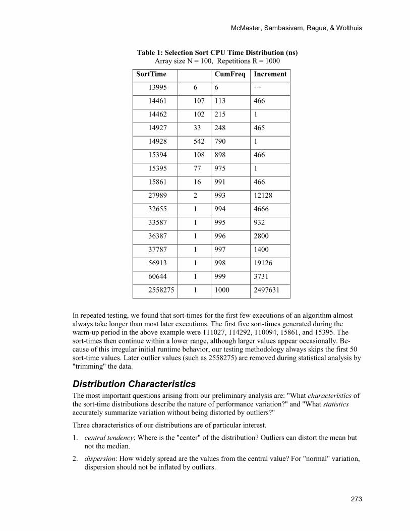
The following selection sort execution time distribution demonstrates features that influenced our research methodology. In this case, the array size is 100, and the number of repetitions is 1000. The total number of repetitions was 1050, but the first 50 "warm-up" values were discarded. A frequency distribution of the retained 1000 sort-times for our Java benchmark program is shown in Table 1.

Several interesting and suggestive features appear in the distribution.

1. The sample of sort-times contains many repeat values. Only 16 distinct values appear in the 1000 repetitions of the sorting algorithm.

2. Most of the high frequency sort-times appear in "pairs", differing by 1 nanosecond. This is probably due to rounding within the Java nanoTime function, which returns an integer.

3. If we consider pairs differing by 1 as a single value, 969 (975 - 6) of the 1000 values in the distribution appear in 3 middle-range sort-times.

4. Considering pairs differing by 1 as a single value, the difference between consecutive pairs is between 466 and 467 (approximately 466.5). We can interpret this difference as the resolution of the clock increment for the nanoTime method.

Oracle's Java documentation (2014) states that the nanoTime method "returns the current value of the most precise available system timer, in nanoseconds." Apparently, the recorded sort-times on our test computer are accurate to about 466.5 nanoseconds. Note that 30 clock increments elapse for the smallest sort-time 13995. In tests on other computers, we observed similar results, but the size of the clock increment was hardware dependent.

5. The mean of the sort-times (17664) is well above the median (14928), which suggests strong positive skewness.

6. The standard deviation of 80458 is greatly inflated by outliers.

7. The largest value (2558275) is clearly an outlier. Based on relative frequency, all values above 15861could be considered as outliers.

McMaster, Sambasivam, Rague, & Wolthuis

273

Table 1: Selection Sort CPU Time Distribution (ns) Array size N = 100, Repetitions R = 1000

SortTime CumFreq Increment

13995 6 6 ---

14461 107 113 466

14462 102 215 1

14927 33 248 465

14928 542 790 1

15394 108 898 466

15395 77 975 1

15861 16 991 466

27989 2 993 12128

32655 1 994 4666

33587 1 995 932

36387 1 996 2800

37787 1 997 1400

56913 1 998 19126

60644 1 999 3731

2558275 1 1000 2497631

In repeated testing, we found that sort-times for the first few executions of an algorithm almost always take longer than most later executions. The first five sort-times generated during the warm-up period in the above example were 111027, 114292, 110094, 15861, and 15395. The sort-times then continue within a lower range, although larger values appear occasionally. Be-cause of this irregular initial runtime behavior, our testing methodology always skips the first 50 sort-time values. Later outlier values (such as 2558275) are removed during statistical analysis by "trimming" the data.

Distribution Characteristics The most important questions arising from our preliminary analysis are: "What characteristics of the sort-time distributions describe the nature of performance variation?" and "What statistics accurately summarize variation without being distorted by outliers?"

Three characteristics of our distributions are of particular interest.

1. central tendency: Where is the "center" of the distribution? Outliers can distort the mean but not the median.

2. dispersion: How widely spread are the values from the central value? For "normal" variation, dispersion should not be inflated by outliers.

Execution Times for Sorting Algorithms

274

3. skewness: How "unbalanced" is the distribution on both sides of the central value? Skewness can be exaggerated by outliers.

Sort-time Central Tendency In this section, we analyze the central tendency of execution time distributions for the five sorting algorithms: selection sort, insertion sort, shell sort, merge sort, and quick sort. For each algorithm, we examine ten array sizes: 100, 200, 300, ..., 1000. We also examine the effect of outliers on central tendency. We include a brief discussion of skewness here because our measures of skew-ness compare the mean to the median.

Median For each sorting algorithm and array size, we want to estimate the center of the distribution of normal sort-times, which does not include outliers. Our main statistics for measuring. central ten-dency are the median and the trimmed mean.

The median is the measure of central tendency least affected by outliers. The usual formula for the median is to average the two middle scores when the sample size is even. To simplify our code, we calculated the median as the lower of the two middle values for even sample sizes. This change had minimal effect on the results, since the sample sizes during our data collection were very large (and the samples contained many duplicate values).

In Table 2, we present the median for each sorting algorithm and array size. The medians are from samples of R = 10000 sort-times generated by our Java program. As we mentioned earlier, to avoid initial outliers, we ran the algorithm 50 times during a "warm-up" period before record-ing the R execution times.

The sort-times are in nanoseconds, but the times are not accurate to the nearest nanosecond. Be-cause each distribution has many duplicate values, the median appears multiple times in each sample. As a result, each median can be restated as the number of "ticks" for the Java nanoTime clock by dividing the time value by 466.5. For example, 138083 / 466.5 = 296.0 (rounded).

Table 2: Sort-time Distribution - Median Size Select Insert Shell Merge Quick

100 14928 6064 6064 9797 6997

200 50381 20992 13995 21926 14928

300 104029 45250 22859 34987 23791

400 177735 78371 32655 49449 32655

500 268702 120823 42918 62511 41984

600 378796 172604 53648 79771 51315

700 507084 233715 64377 93300 60645

800 655430 303690 75572 108227 70441

900 821037 382995 86768 121756 80237

1000 1003903 470696 97498 138083 90034

McMaster, Sambasivam, Rague, & Wolthuis

275

If the size variable is N, then each column can be correlated with N2 and NlogN to estimate the order-of-growth of the algorithm. For selection sort and insertion sort, the correlation with N2 is 0.99988 and 0.99998, respectively. This matches the known order-of-growth for these algorithms.

Selection sort and insertion sort have the same order-of-growth, but not the same execution speed. Order-of-growth ignores constants. Our data indicate that insertion sort takes less than half the time as selection sort. This fact is ignored by the usual order-of-growth models.

Over our limited range of array sizes, the remaining three algorithms correlate higher than 0.999 with NlogN. This is consistent with the order-of-growth for merge sort and quick sort. The growth rate for shell sort depends on the initial gap sequence used in the algorithm.

From the data in Table 2, shell sort and quick sort are approximately the same speed until the ar-ray size reaches 500. Beyond that point, quick sort becomes slightly faster. Both quick sort and shell sort are noticeably faster than merge sort for all array sizes.

Outliers and Skewness The measure of central tendency provided by the median in our data is limited in precision by the size of the nanoTime clock increment. Means have a smaller standard error than medians, but the accuracy of the mean for estimating the center of the "normal" values is substantially diminished by outliers.

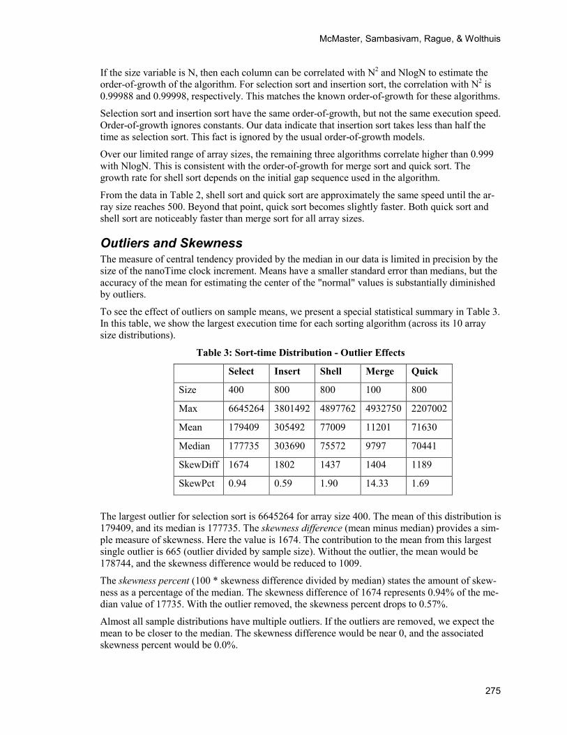
To see the effect of outliers on sample means, we present a special statistical summary in Table 3. In this table, we show the largest execution time for each sorting algorithm (across its 10 array size distributions).

Table 3: Sort-time Distribution - Outlier Effects

Select Insert Shell Merge Quick

Size 400 800 800 100 800

Max 6645264 3801492 4897762 4932750 2207002

Mean 179409 305492 77009 11201 71630

Median 177735 303690 75572 9797 70441

SkewDiff 1674 1802 1437 1404 1189

SkewPct 0.94 0.59 1.90 14.33 1.69

The largest outlier for selection sort is 6645264 for array size 400. The mean of this distribution is 179409, and its median is 177735. The skewness difference (mean minus median) provides a sim-ple measure of skewness. Here the value is 1674. The contribution to the mean from this largest single outlier is 665 (outlier divided by sample size). Without the outlier, the mean would be 178744, and the skewness difference would be reduced to 1009.

The skewness percent (100 * skewness difference divided by median) states the amount of skew-ness as a percentage of the median. The skewness difference of 1674 represents 0.94% of the me-dian value of 17735. With the outlier removed, the skewness percent drops to 0.57%.

Almost all sample distributions have multiple outliers. If the outliers are removed, we expect the mean to be closer to the median. The skewness difference would be near 0, and the associated skewness percent would be 0.0%.

Execution Times for Sorting Algorithms

276

For the original (untrimmed) sample data across sorting algorithm and array size, the largest skewness difference was 6822. This was for merge sort with array size 1000. The largest skew-ness percent was a hefty 18.01% for merge sort with array size 300.

To remove outliers, we initially trimmed each sample by removing the top and bottom 1% of the sort-times. In doing so, the largest skewness difference dropped to 1953, again for merge sort with array size 1000. The largest skewness percent decreased significantly to 1.81% for merge sort with array size 100.

When we removed the top and bottom 5% of each sample, the largest skewness difference was 549 for selection sort on arrays of size 900. Skewness difference for the other sorting algorithms was always under 250. All but two of the differences were below the resolution of the nanoTime clock. The largest skewness percent was 1.38% for merge sort with array size 100. With 5% trimming, skewness was essentially eliminated for all sort algorithms and array sizes.

Note that the median remains unchanged for all trimmed samples because we removed the same number of values from both ends of the sort-time distribution.

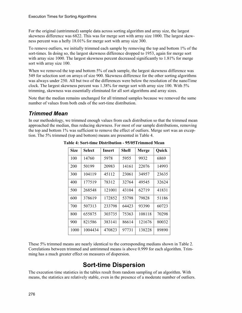
Trimmed Mean In our methodology, we trimmed enough values from each distribution so that the trimmed mean approached the median, thus reducing skewness. For most of our sample distributions, removing the top and bottom 1% was sufficient to remove the effect of outliers. Merge sort was an excep-tion. The 5% trimmed (top and bottom) means are presented in Table 4.

Table 4: Sort-time Distribution - 95/05Trimmed Mean

Size Select Insert Shell Merge Quick

100 14760 5978 5955 9932 6869

200 50199 20983 14161 22076 14993

300 104119 45112 23061 34957 23635

400 177519 78312 32764 49545 32624

500 268548 121001 43104 62719 41831

600 378619 172852 53798 79828 51186

700 507313 233798 64423 93390 60723

800 655875 303735 75363 108118 70298

900 821586 383141 86614 121676 80032

1000 1004434 470823 97731 138228 89890

These 5% trimmed means are nearly identical to the corresponding medians shown in Table 2. Correlations between trimmed and untrimmed means is above 0.999 for each algorithm. Trim-ming has a much greater effect on measures of dispersion.

Sort-time Dispersion The execution time statistics in the tables result from random sampling of an algorithm. With means, the statistics are relatively stable, even in the presence of a moderate number of outliers.

McMaster, Sambasivam, Rague, & Wolthuis

277

The same claim cannot be made for measures of dispersion. Statistics that measure dispersion can be greatly distorted when even a few outliers appear in the sample.

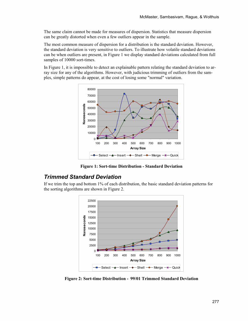
The most common measure of dispersion for a distribution is the standard deviation. However, the standard deviation is very sensitive to outliers. To illustrate how volatile standard deviations can be when outliers are present, in Figure 1 we display standard deviations calculated from full samples of 10000 sort-times.

In Figure 1, it is impossible to detect an explainable pattern relating the standard deviation to ar-ray size for any of the algorithms. However, with judicious trimming of outliers from the sam-ples, simple patterns do appear, at the cost of losing some "normal" variation.

0

10000

20000

30000

40000

50000

60000

70000

80000

100 200 300 400 500 600 700 800 900 1000

Array Size

Nan

osec

onds

Select Insert Shell Merge Quick

Figure 1: Sort-time Distribution - Standard Deviation

Trimmed Standard Deviation If we trim the top and bottom 1% of each distribution, the basic standard deviation patterns for the sorting algorithms are shown in Figure 2.

0

2500

5000

7500

10000

12500

15000

17500

20000

22500

100 200 300 400 500 600 700 800 900 1000

Array Size

Nan

osec

onds

Select Insert Shell Merge Quick

Figure 2: Sort-time Distribution - 99/01 Trimmed Standard Deviation

Execution Times for Sorting Algorithms

278

For each algorithm, the trimmed standard deviation increases steadily with the sample size. Merge sort has a break in the pattern when the array size reaches 900. At this point, the standard deviation increases sharply. One possible reason for this abrupt change is that merge sort requires extra memory. Java's runtime garbage collection eventually has to do much more work, which increases the number of outliers.

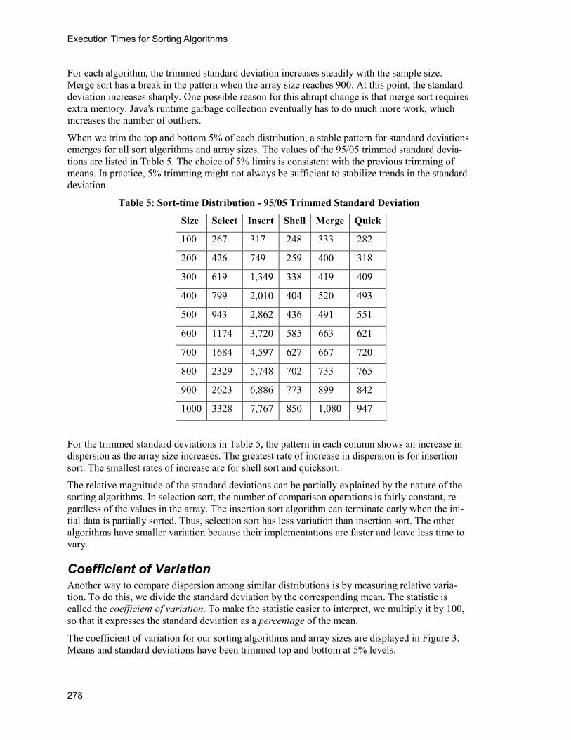
When we trim the top and bottom 5% of each distribution, a stable pattern for standard deviations emerges for all sort algorithms and array sizes. The values of the 95/05 trimmed standard devia-tions are listed in Table 5. The choice of 5% limits is consistent with the previous trimming of means. In practice, 5% trimming might not always be sufficient to stabilize trends in the standard deviation.

Table 5: Sort-time Distribution - 95/05 Trimmed Standard Deviation

Size Select Insert Shell Merge Quick

100 267 317 248 333 282

200 426 749 259 400 318

300 619 1,349 338 419 409

400 799 2,010 404 520 493

500 943 2,862 436 491 551

600 1174 3,720 585 663 621

700 1684 4,597 627 667 720

800 2329 5,748 702 733 765

900 2623 6,886 773 899 842

1000 3328 7,767 850 1,080 947

For the trimmed standard deviations in Table 5, the pattern in each column shows an increase in dispersion as the array size increases. The greatest rate of increase in dispersion is for insertion sort. The smallest rates of increase are for shell sort and quicksort.

The relative magnitude of the standard deviations can be partially explained by the nature of the sorting algorithms. In selection sort, the number of comparison operations is fairly constant, re-gardless of the values in the array. The insertion sort algorithm can terminate early when the ini-tial data is partially sorted. Thus, selection sort has less variation than insertion sort. The other algorithms have smaller variation because their implementations are faster and leave less time to vary.

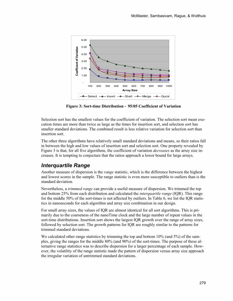
Coefficient of Variation Another way to compare dispersion among similar distributions is by measuring relative varia-tion. To do this, we divide the standard deviation by the corresponding mean. The statistic is called the coefficient of variation. To make the statistic easier to interpret, we multiply it by 100, so that it expresses the standard deviation as a percentage of the mean.

The coefficient of variation for our sorting algorithms and array sizes are displayed in Figure 3. Means and standard deviations have been trimmed top and bottom at 5% levels.

McMaster, Sambasivam, Rague, & Wolthuis

279

-

1.00

2.00

3.00

4.00

5.00

6.00

100 200 300 400 500 600 700 800 900 1000

Array Size

Coef

ficie

nt o

f Var

iatio

n

Select Insert Shell Merge Quick

Figure 3: Sort-time Distribution - 95/05 Coefficient of Variation

Selection sort has the smallest values for the coefficient of variation. The selection sort mean exe-cution times are more than twice as large as the times for insertion sort, and selection sort has smaller standard deviations. The combined result is less relative variation for selection sort than insertion sort.

The other three algorithms have relatively small standard deviations and means, so their ratios fall in between the high and low values of insertion sort and selection sort. One property revealed by Figure 3 is that, for all five algorithms, the coefficient of variation decreases as the array size in-creases. It is tempting to conjecture that the ratios approach a lower bound for large arrays.

Interquartile Range Another measure of dispersion is the range statistic, which is the difference between the highest and lowest scores in the sample. The range statistic is even more susceptible to outliers than is the standard deviation.

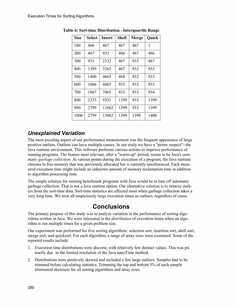
Nevertheless, a trimmed range can provide a useful measure of dispersion. We trimmed the top and bottom 25% from each distribution and calculated the interquartile range (IQR). This range for the middle 50% of the sort-times is not affected by outliers. In Table 6, we list the IQR statis-tics in nanoseconds for each algorithm and array size combination in our design.

For small array sizes, the values of IQR are almost identical for all sort algorithms. This is pri-marily due to the coarseness of the nanoTime clock and the large number of repeat values in the sort-time distributions. Insertion sort shows the largest IQR growth over the range of array sizes, followed by selection sort. The growth patterns for IQR are roughly similar to the patterns for trimmed standard deviations.

We calculated other range statistics by trimming the top and bottom 10% (and 5%) of the sam-ples, giving the ranges for the middle 80% (and 90%) of the sort-times. The purpose of these al-ternative range statistics was to describe dispersion for a larger percentage of each sample. How-ever, the volatility of the range statistic made the pattern of dispersion versus array size approach the irregular variation of untrimmed standard deviations.

Execution Times for Sorting Algorithms

280

Table 6: Sort-time Distribution - Interquartile Range

Size Select Insert Shell Merge Quick

100 466 467 467 467 1

200 467 933 466 467 466

300 933 2332 467 933 467

400 1399 3265 467 932 933

500 1400 4665 468 932 933

600 1866 6065 933 933 933

700 1867 7465 933 933 934

800 2333 9331 1399 933 1399

900 2799 11662 1399 933 1399

1000 2799 13062 1399 1399 1400

Unexplained Variation The most puzzling aspect of our performance measurement was the frequent appearance of large positive outliers. Outliers can have multiple causes. In our study we have a "prime suspect"--the Java runtime environment. This software performs various actions to improve performance of running programs. The feature most relevant, after a "warm-up" period, seems to be Java's auto-matic garbage collection. At various points during the execution of a program, the Java runtime chooses to free memory that was previously allocated but is currently unreferenced. Each meas-ured execution time might include an unknown amount of memory reclamation time in addition to algorithm processing time.

The simple solution for running benchmark programs with Java would be to turn off automatic garbage collection. That is not a Java runtime option. Our alternative solution is to remove outli-ers from the sort-time data. Sort-time statistics are affected most when garbage collection takes a very long time. We treat all suspiciously large execution times as outliers, regardless of cause.

Conclusions The primary purpose of this study was to analyze variation in the performance of sorting algo-rithms written in Java. We were interested in the distribution of execution times when an algo-rithm is run multiple times for a given problem size.

Our experiment was performed for five sorting algorithms: selection sort, insertion sort, shell sort, merge sort, and quicksort. For each algorithm, a range of array sizes were examined. Some of the reported results include:

1. Execution time distributions were discrete, with relatively few distinct values. This was pri marily due to the limited resolution of the Java nanoTime method.

2. Distributions were positively skewed and included a few large outliers. Samples had to be trimmed before calculating statistics. Trimming the top and bottom 5% of each sample eliminated skewness for all sorting algorithms and array sizes.

McMaster, Sambasivam, Rague, & Wolthuis

281

3. For all sorting algorithms, the mean sort-time increased as the array size increased. The dif ferent observed rates of increase were consistent with known order-of-growth models.

4. For each algorithm, the trimmed standard deviation of sort-times increased with array size. The algorithms differed in the amount of variation and the pattern of growth. The patterns can be interpreted in terms of the internal structure of each algorithm.

5. For each algorithm, the standard deviation grew at a slower rate than the mean. This was demonstrated by a decreasing coefficient of variation as the array size increased.

Several conclusions can be drawn from our results. First, sort-time variation is an important fac-tor in systems with real-time constraints. Second, sort-time variation is less important for large arrays because the amount of variation is small relative to the mean. Third, beware of outliers, especially when using the Java runtime environment to run benchmarks. Including a suitable warm-up period and employing effective trimming strategies on sample execution times can less-en the influence of outliers.

Future Research Good research generates more questions than it answers. This is true for this study. Our planned future research activities include:

1. Examine sort-time variation for larger array sizes to see if distribution patterns persist.

2. Use our research approach on algorithms written in other programming languages, especially with fully-compiled programs. An obvious next language is C++. However, C++ provides different timer functions in alternative operating environments.

3. Examine the variation in execution times when the data is non-random or constant. In particu- lar, measure the variation when best-case and worst-case examples are run repeatedly.

4. Study the effect of rounding errors introduced by the coarseness of Java's nanoTime method. This research would examine how Oracle utilizes "the most precise available system timer" in different hardware and software environments.

References Aho, A. (1974). The design and analysis of computer algorithms. Addison-Wesley.

Aho, A., Ullman, J., & Hopcroft, J. (1983). Data structures and algorithms. Addison-Wesley.

Boyer, B. (2008). Robust Java benchmarking, Part 1: Issues. IBM DeveloperWorks, 24 June 2008.

Cormen, T. H., Leiserson, C. E., Rivest, R. L., & Stein, C. (2009). Introduction to algorithms (3rd ed). MIT Press.

Goetz, B. (2004). Java theory and practice: Dynamic compilation and performance measurement. IBM De-veloperWorks, 21 December 2004.

Helman, D., Bader, D., & JaJa, J. (1998). A randomized parallel sorting algorithm with an experimental study. Journal of Parallel and Distributed Computing, 52(1), July 10.

Kleinberg, J., & Tardos, E. (2006). Algorithm design. Addison-Wesley.

Knuth, D. (1998). The art of computer programming: Volume 3: Sorting and searching (2nd ed). Addison-Wesley Professional.

Koffman, E., & Wolfgang, P. (2010). Data structures: Abstraction and design using Java (2nd ed). Wiley.

Lafore, R. (2003). Data structures and algorithms in Java (2nd ed). Sams Publishing.

Main, M., & Savich, W. (2010). Data structures and other objects using C++. Prentice Hall.

Execution Times for Sorting Algorithms

282

Musselman, R. (2007). Robustness: A better measure of algorithm performance. Thesis, Naval Postgradu-ate School, Monterey, CA.

Oracle (2014). java.lang class system. Retrieved February 9, 2015, from http://docs.oracle.com

Sedgewick, R., & Wayne, K. (2011). Algorithms (4th ed). Addison-Wesley.

Wicht, B. (2011). Java micro-benchmarking: How to write correct benchmarks. Retrieved February 9, 2015, from http://www.javacodegeeks.com/2011/09/

Biographies Dr. Kirby McMaster is retired from the Computer Science Depart-ment at Weber State University. To remain active, he has been a visit-ing professor at several colleges and universities. His primary research interests are in database systems, software engineering, and frame-works for Mathematics and Computer Science.

Dr. Samuel Sambasivam is Chair Emeritus and Professor of Comput-er Science, and Director of Computer Science Programs at Azusa Pa-cific University. His research interests include optimization methods, expert systems, client/server applications, database systems, and genet-ic algorithms. He served as a Distinguished Visiting Professor of Computer Science at the United States Air Force Academy in Colorado Springs, Colorado for a year. He has conducted extensive research, written for publications, and delivered presentations in Computer Sci-ence, data structures, and Mathematics. He is a voting member of the ACM.

Dr. Brian Rague is Professor and Chair of the Computer Science De-partment at Weber State University. His research interests involve par-allel computing, programming languages, and opportunities for crea-tive software engineering in the fields of education, biomedicine and physics.

McMaster, Sambasivam, Rague, & Wolthuis

283

Stuart L. Wolthuis is Assistant Professor and Chair of the Computer & Information Sciences Department at Brigham Young University--Hawaii. His teaching focus includes software engineering, HCI, and information assurance. He brings almost 24 years of service in the USAF to the classroom with real world experiences as a program man-ager and software engineer. When not enjoying Hawaii’s great out-doors, his research interests include melding together information sys-tems and marine biology. His current project, Ocean View, will link land-locked educators and students to live underwater ocean views via an educational website.