A Novel Calibration Method for Industrial AGVs

Fabjan Kallasia, Dario Lodi Rizzinia, Fabio Olearia,b, MassimilianoMagnanib, Stefano Casellia

aRobotics and Intelligent Machines Laboratory, Department of Information Engineering,University of Parma, 43124, Italy

bElettric80 S.p.A. 42030 Viano (RE), Italy

Abstract

We propose a novel calibration method for industrial Automated Guided Ve-hicles (AGVs) adopting the tricycle wheeled robot model and equipped withan on-board exteroceptive sensor. The method simultaneously estimates thecalibration parameters for the odometry and the exteroceptive sensor usingonly the input commands and the sensor egomotion of the robot while execut-ing segment paths. Two AGV models, both relevant to industrial practice,are considered: the standard tricycle model and an asymmetric one thattakes into account the different weight distribution in forward and backwardmotions typical of industrial AGVs. The parameters of the standard modelcomprise the steering offset and driving scale, which measure the angular off-set of the tricycle steering wheel and the distance increment correspondingto an encoder tick, and the three parameters representing the sensor pose.The asymmetric model adopts different values for the steering offset in for-ward and backward motions to account for the different weight distribution.Closed-form or compact solutions are provided for both problem formula-tions. The observability of the calibration procedure is also formally proved.The proposed automated calibration procedure has been implemented on in-dustrial AGVs, leading to estimation of the parameters in about 12 minutes,a significant improvement compared with one hour or more required by man-ual AGV calibration. Experiments with AGVs of various sizes in warehouseshave assessed the effectiveness and numerical stability of the proposed ap-proach. The precision of calibration parameters has been found to be about0.1◦ for angles and 6mm for positions. Parameters obtained via the proposedautomated calibration procedure have allowed different AGVs to accuratelystop at the desired operation points.

Preprint submitted to Robotics and Autonomous Systems May 11, 2017

Keywords: Industrial mobile robots, extrinsic calibration, odometrycalibration.

1. Introduction

A common requirement of industrial robotic systems is the capabilityto repeat operations with adequate precision. Precision is a fundamen-tal requirement of traditional assembly lines where products are moved byrobot manipulators and other devices, as well as of warehouse logistic sys-tems exploiting automated guided vehicles (AGVs). AGVs are mobile robotsequipped with forks or other grasping devices to transport pallets and mate-rials from a warehouse location to another according to assigned productionpolicies. Since the exact location of each pallet is registered into a database,AGVs estimate their pose using an exteroceptive sensor, often a navigationrange finder and artificial reflectors, to accurately pick and drop items. Fig-ure 1 shows a typical AGV in an industrial setting.

The accuracy of robotic systems depends on the estimation of parametersthat describe their motion and configuration. These parameters either rep-resent the robot internal state or relate other sensors or devices to the robot.Respectively, the former are called intrinsic parameters and the latter ex-trinsic parameters. Intrinsic parameters usually describe the relationshipbetween the actuators state and the robot kinematics. Extrinsic parametersrelate the sensor measurements to the robot reference frame. The correctassessment of the AGV parameters affects its navigation accuracy, namelyits odometry and localization. Hence, the aim of calibration is the accurateestimation of these parameters.

A standard approach for mobile robot calibration is to compare the ex-pected motion of the robot from some input commands with the observedtrajectory. Currently, industrial vehicles are calibrated through a manualprocedure requiring the intervention of an operator to measure the effectivetrajectory. Each parameter is updated in sequence and multiple iterationsare often needed. This is a tedious process requiring at least one hour for eachAGV. Its accuracy largely depends on the skills and experience of the opera-tor performing the calibration. Moreover, consistency of manual calibrationwith multiple, possibly different AGVs operating in the same warehouse is of-ten questionable and can lead to AGVs exhibiting slightly different behaviorfor the same nominal position.

2

Since AGVs are usually equipped with one or more sensors for localizationand navigation (e.g. a laser scanner) that can estimate the sensor egomotion,on-board sensors can be used to estimate the effective motion of the vehicle.Knowledge of the relative pose of the on-board sensor w.r.t. the robot frameis required to obtain the real robot trajectory using such sensor. The sen-sor relative pose can be assessed from its egomotion while the robot moveson a known trajectory. Thus, a completely automated calibration methodshould estimate both intrinsic and extrinsic parameters. A more efficient andaccurate procedure can bring remarkable improvements to industrial appli-cations, including the faster setup of an AGV fleet and the possibility for lessexpensive and more frequent recalibration to compensate parameter changesover time due to mechanical wear, vibrations, and collisions.

Research has addressed several formulations of calibration problems fordifferent robotic systems, including the calibration of multi-sensor systemsand robot odometry [1, 2, 3, 4, 5, 6, 7, 8, 9, 10, 11, 12, 13, 14, 15, 16,17, 18, 19, 20, 21, 22, 23, 24, 25, 26, 27, 28]. Many works focus on theestimation of either intrinsic [2, 3, 4, 5, 6, 7, 29, 8, 9, 10, 11, 23, 24, 25] orextrinsic parameters [12, 13, 14, 15, 16, 17, 18, 19, 20, 21, 22, 26, 27, 28].Recently, an algorithm for the complete calibration of a mobile robot hasbeen proposed [1]. The kinematic model considered in works addressingmobile robot calibration [1, 2, 3, 4, 5, 6, 7, 10, 11] is the popular differentialdrive. The proposed techniques therefore are mostly suited for a laboratoryrobotic platform rather than industrial vehicles, since AGVs seldom adoptsuch kinematic configuration. Furthermore, these approaches do not take intoaccount practical and numerical issues arising in industrial setups. Indeed,AGVs operate in large scale environments where odometric errors due to longtravelled distances do occur. Moreover, AGVs are usually designed accordingto a tricycle structure consisting of a steering actuated front wheel and twopassive back wheels, due the simplicity of such self-standing configuration aswell as its suitability for fetching, carrying, and depositing heavy loads. Thetricycle robot, which is kinematically equivalent to a bicycle [29, p. 482], hasbeen largely ignored in the investigation of calibration. To our knowledge,no approach has addressed so far automatic calibration of both intrinsic andextrinsic parameters of tricycle robots equipped with a sensor.

In this paper, we present the first method for simultaneous intrinsic andextrinsic calibration of tricycle robots equipped with a sensor like a planarlaser scanner. Parameter estimation is achieved by comparing the motionexpected from kinematic equations and the sensor egomotion. Two differ-

3

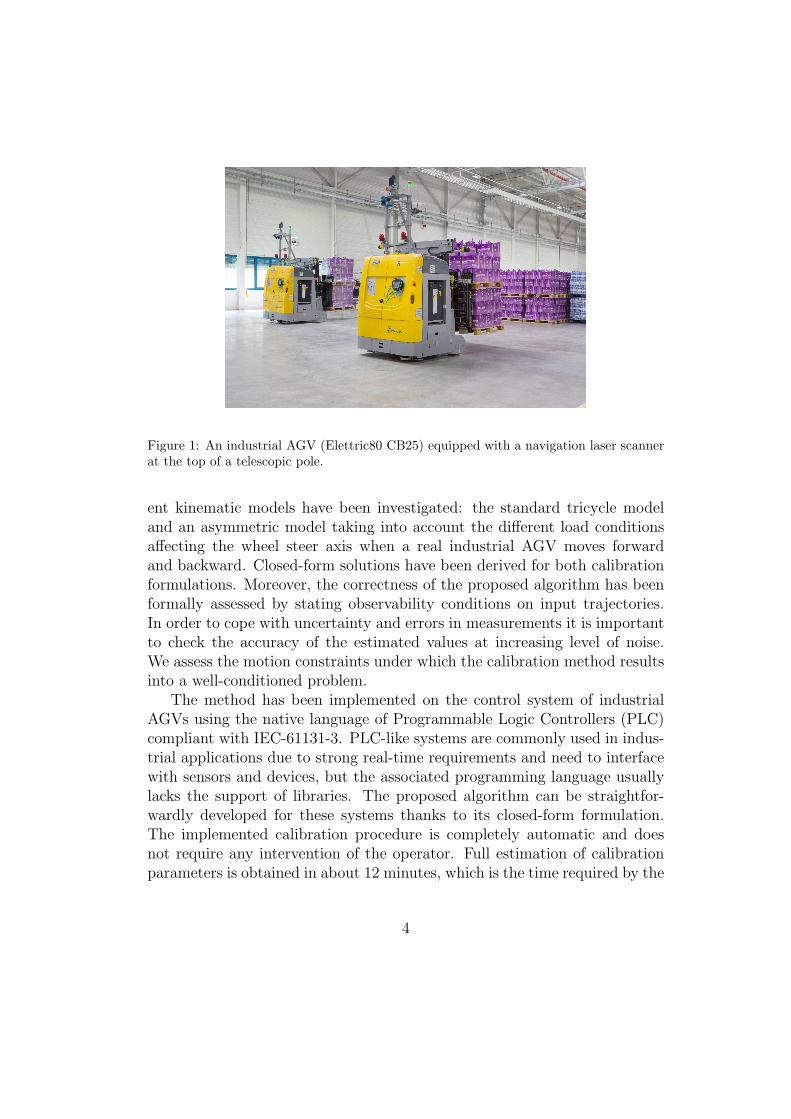
Figure 1: An industrial AGV (Elettric80 CB25) equipped with a navigation laser scannerat the top of a telescopic pole.

ent kinematic models have been investigated: the standard tricycle modeland an asymmetric model taking into account the different load conditionsaffecting the wheel steer axis when a real industrial AGV moves forwardand backward. Closed-form solutions have been derived for both calibrationformulations. Moreover, the correctness of the proposed algorithm has beenformally assessed by stating observability conditions on input trajectories.In order to cope with uncertainty and errors in measurements it is importantto check the accuracy of the estimated values at increasing level of noise.We assess the motion constraints under which the calibration method resultsinto a well-conditioned problem.

The method has been implemented on the control system of industrialAGVs using the native language of Programmable Logic Controllers (PLC)compliant with IEC-61131-3. PLC-like systems are commonly used in indus-trial applications due to strong real-time requirements and need to interfacewith sensors and devices, but the associated programming language usuallylacks the support of libraries. The proposed algorithm can be straightfor-wardly developed for these systems thanks to its closed-form formulation.The implemented calibration procedure is completely automatic and doesnot require any intervention of the operator. Full estimation of calibrationparameters is obtained in about 12 minutes, which is the time required by the

4

AGV to perform an adequate number of motions. Experiments performedin real industrial setups, including production warehouses, have shown thatthe values computed with the proposed method are stable and yield accurateAGV navigation capabilities.

2. Related Work

Calibration of mobile robots has been addressed from several points ofview by academic research. Calibration may refer only to the estimationof the robot kinematic parameters used in odometry computation or mayinclude the relationship between the robot and its sensors. During the lasttwo decades, research has addressed the assessment of mobile robot intrinsicparameters, of the extrinsic parameters of a sensor mounted on it, or of bothsets of parameters.

2.1. Manual Odometry Calibration

Most of odometry calibration literature is devoted to differential driverobots. Several wheeled mobile robots are designed with a differential driveactuation system due to the simplicity of such configuration. In particular,the parameters to be estimated are the two wheel diameters and the wheel-base distance. Borenstein et al. [2] likely proposed the first specific calibrationmethod for differential drive robots, the UMBmark. This technique requiresthe robot to move along a square trajectory in both directions, clockwiseand counterclockwise, and measures the displacement between the final andthe starting points after the execution of a loop to compute the correctionfactors of wheel-base and wheel diameters. This approach has been appliedalso to other kinematic models such as the car-like [8] or the tricycle [9],but mainstream research has been focused on differential drive. Odometrycalibration is coupled with the calibration of internal sensors like gyroscopesand IMUs used to correct odometry [9]. Currently, similar procedures areoften used to estimate odometric parameters in industrial practice: the robotfollows specific paths (typically straight lines or loops) and the distance be-tween the expected path with initial parameters and the measured one isused to correct parameters. Such distance is measured either manually orthrough an external absolute positioning system. Moreover, each calibrationparameter is estimated sequentially after performing a specific step, insteadof performing a simultaneous optimization. The separate assessment of eachparameter is usually less accurate.

5

2.2. Calibration based on Filtering Methods

In several works the calibration problem has been addressed using thesame Bayesian filtering algorithms adopted for robot localization. The sys-tem state consists of both the robot pose and its kinematic parameters, al-though the latter do not change or slowly change over the time. Larsen etal. [3] and Martinelli et al. [5] present augmented Extended Kalman Filter(AEKF) algorithms that simultaneously localize and calibrate the mobilerobot. The method illustrated in [10] jointly uses a gyroscope, the wheel en-coders, and a GPS unit in a Kalman filter to correct systematic errors. In [11]a simultaneous SLAM and calibration algorithm specific for feature maps ispresented. These works are designed for differential drive and, thus, cannotbe applied to other drive models. Furthemore, they do not simultaneouslyestimate the intrinsic and extrinsic parameters.

Calibration of on-board sensors through EKF is a rather straightforwardstep. Extrinsic calibration parameters usually describe the pose of a sen-sor w.r.t. a common reference frame fixed on the robot. The EKF has beenapplied to the calibration of different kinds of sensors or of heterogeneous sen-sors. Early examples of camera calibration techniques based on Kalman filtercan be found in [14], the latter specific for eye-in-hand cameras. The extrinsicparameters of laser scanners are estimated by tracking moving targets [15] orby comparing the robot pose evolution and the landmark measurements [16].Foxlin [12] proposed a general EKF framework that allows localization andcalibration of multiple sensors. Martinelli et al. [17] describe an EKF forassessing the parameters of a camera mounted on a robot during the robotmotion. This work presents one of the first observability analysis for a cal-ibration problem based on discrete-time system state evolution, which hasbeen further developed in [4]. The authors also provide an observability anal-ysis proving the formal correctness of the calibration process. Mirzaei andRoumeliotis [18] illustrate a method for calibrating a camera and an inertialsensor using a Kalman filter. The works discussed above are designed onlyto estimate the pose of one or more sensors w.r.t. the robot or to anothersensor.

2.3. Calibration based on Least-square Optimization

Least square optimization has been used to estimate both intrinsic andextrinsic parameters. Historically, optimization is the earliest approach tospecific calibration problems in robotics and computer vision like pinholesingle and stereo cameras [13, 19] and eye-in-hand cameras [20, 21]. These

6

techniques usually compute a closed-form initial estimation based on a sim-plified model and next refine this estimation by numerically optimizing theerror associated to more complex sensor models taking into account opticaldistortions, offsets, etc. Calibration of heterogeneous sensor systems requiresa target that is observable from different sensor domains and geometries.Zhang and Pless [22] illustrate a method for a planar range finder and acamera exploiting a planar checkerboard.

In mobile robotics, the extrinsic or intrinsic calibration based on least-square optimization is more recent. Sometimes the function to be optimizedis obtained from a stochastic formulation of the problem. Roy and Thrun [23]proposed the computation of the intrinsic parameters according to maximumlikelihood criterion: the robot builds a map while moving, and estimates thelikelihood function to be maximized. Antonelli et al. [6, 7] focus on the differ-ential drive model and on the linear relationship between the observed robotmotion and the quantities depending on intrinsic parameters. The calibra-tion is achieved by solving a linear optimization problem and a bound on thecalibration error is provided. An analysis of odometry error propagation isdescribed in [24]. The work in [25] presents a calibration framework based ona graphical model formulation. The framework is rather general, but it doesnot explicitly consider the robot model and is potentially prone to conver-gence problems and inaccuracies. Underwood et al.[26] and Brookshire andTeller [27] address the calibration of multiple sensors mounted on a mobilerobot using least-square optimization. The latter work has been extendedfrom coplanar sensors to 3D range sensors like depth cameras [28].

The only complete odometry and sensor calibration method is reportedin [1]. The estimation of intrinsic and extrinsic parameters is decoupledinto two steps. The intrinsic calibration is the straightforward applicationof the differential drive solution [7]. The extrinsic parameters are obtainedby comparing the robot motion and the sensor egomotion. The closed-formsolution for extrinsic parameters proposed in [1] is dependent from the intrin-sic calibration parameters. Such method cannot be used for the calibrationof industrial AGVs, which are designed according to the tricycle kinematicmodel and not to the differential drive one.

7

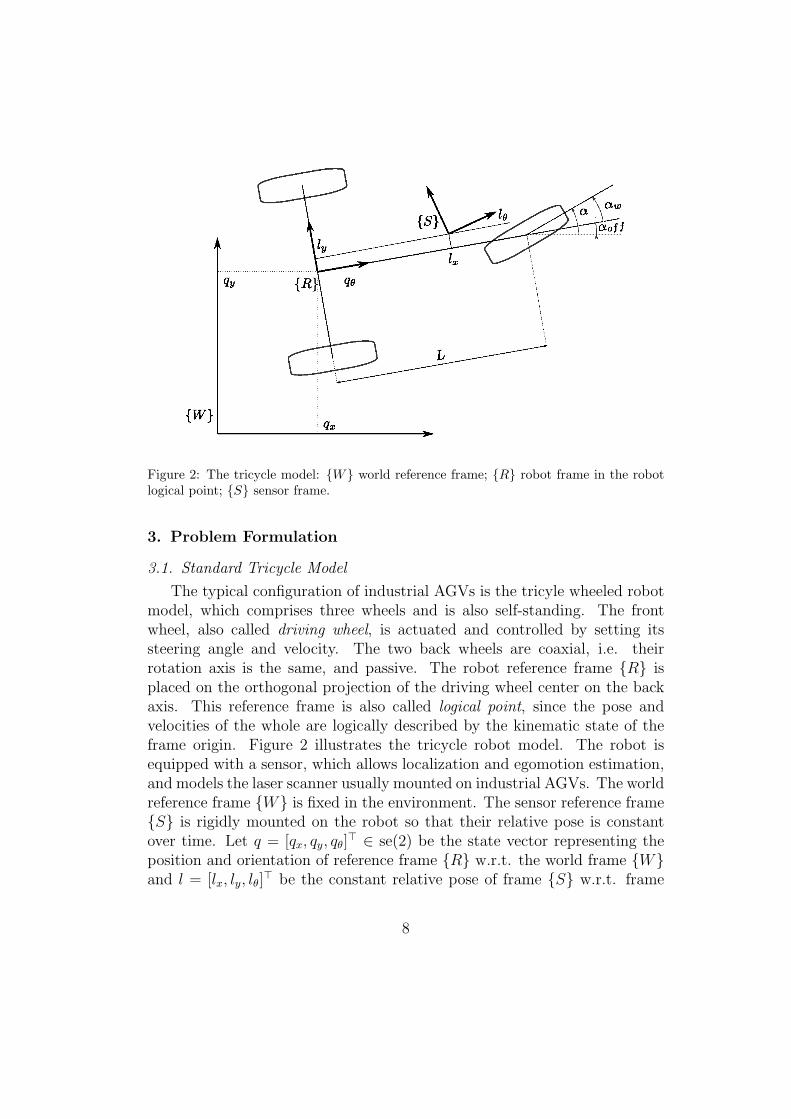
Figure 2: The tricycle model: {W} world reference frame; {R} robot frame in the robotlogical point; {S} sensor frame.

3. Problem Formulation

3.1. Standard Tricycle Model

The typical configuration of industrial AGVs is the tricyle wheeled robotmodel, which comprises three wheels and is also self-standing. The frontwheel, also called driving wheel, is actuated and controlled by setting itssteering angle and velocity. The two back wheels are coaxial, i.e. theirrotation axis is the same, and passive. The robot reference frame {R} isplaced on the orthogonal projection of the driving wheel center on the backaxis. This reference frame is also called logical point, since the pose andvelocities of the whole are logically described by the kinematic state of theframe origin. Figure 2 illustrates the tricycle robot model. The robot isequipped with a sensor, which allows localization and egomotion estimation,and models the laser scanner usually mounted on industrial AGVs. The worldreference frame {W} is fixed in the environment. The sensor reference frame{S} is rigidly mounted on the robot so that their relative pose is constantover time. Let q = [qx, qy, qθ]

⊤ ∈ se(2) be the state vector representing theposition and orientation of reference frame {R} w.r.t. the world frame {W}and l = [lx, ly, lθ]

⊤ be the constant relative pose of frame {S} w.r.t. frame

8

{R}. The kinematic model that describes the evolution of state vector q overtime is

q =

vlp cos (qθ)vlp sin (qθ)

ωlp

(1)

The state vector and all the variables that depend on time will be sometimesexplicitly written as a function of time, i.e. q(t). Although the linear andangular velocities vlp and ωlp are convenient to describe the motion of thelogical point, the real controls for the tricycle robot are set on the frontsteering wheel, whose dynamic configuration is described by its linear velocityvw and its steering angle αw. The steering wheel state is controlled by twomotors, one for rotating the wheel and the other for steering, and monitoredby the corresponding encoders.

The distance travelled by the wheel is proportional to the number of ticksnw counted by the driving encoder. The driving scale sw is a constant thatbinds the distance travelled by the robot to the rotation of the wheel. Thedriving scale depends on the wheel radius (which changes in time as the wheelwears out), on the transmission gears, and on the angular resolution of theencoder. Hence, the wheel linear velocity vw can be written as the productof the driving scale sw and the derivative of tick number in time nw.

The robot rotation velocity depends on the wheelbase L, which is thedistance between the origin of reference frame {R} and the steering wheelaxis, and on the steering angle αw (see Figure 2). In industrial practice, thewheelbase is assumed to be accurately known from the mechanical design.The steering wheel direction for αw = 0 is orthogonal to the back wheel axisand the robot moves on a straight line. The encoder of the motor controllingthe steer measures the steering angle α w.r.t. the encoder reference angle.Unfortunately, it is very difficult to mount the encoder such that its referenceangle is perfectly aligned with the straight direction. Thus, there is a steeroffset αoff between the measured steering angle α w.r.t. the reference angleand αw, so that αw = α + αoff as shown in Figure 2. Thus, the linear andangular velocities in equation (1) can be written as

vlp = vw cosαw = sw nw cos (α + αoff ) (2)

ωlp =vw sinαw

L=sw nw sin (α + αoff )

L(3)

The range finder mounted on the robot is such that the scanning planeis parallel to the ground plane. Hence, the sensor pose s(t) w.r.t. the world

9

reference frame {W} is conveniently described by the robot pose q(t) and therelative pose of the sensor l = [lx, ly, lθ]

⊤ ∈ se(2). The relationships betweenl, q(t) and the other poses can be expressed using standard compounding andinversion operators on special Euclidean Lie algebra se(2), respectively ⊕ and⊖ [30]. Furthermore, the symbol R (·) refers, henceafter, both to the mapfrom an angle β ∈ S1 to the corresponding rotation matrix of R (β) ∈ SO(2)and to the map from a vector b ∈ R

2 to a skew matrix R (b) ∈ R2×2 defined

respectively as

R (β) ,[cos β − sin βsin β cos β

]

, R (b) ,[bx −byby bx

]

(4)

This abuse of notation allows us to write compact formulas and to straight-forwardly compute the expressions. The position of the sensor is then equalto s(t) = q(t) ⊕ l. The measurement values of actuators and sensors areacquired at given sampling times t1, . . . , tk.

The problem addressed in this paper is the estimation of the followingparameters:

• intrinsic parameters : the driving scale of the wheel sw, which relatesthe encoder ticks and the linear velocity, and the steering offset angleαoff ;

• extrinsic parameters : the laser scanner pose parameters l = [lx, ly, lθ]⊤.

The available data are the relative motions of the robot and the laserscanner frames at the sample times tk with k = 0, . . . , n. The choice ofthe number of samples is formally discussed in section 5 and experimentallyassessed in section 6. In particular, the relative robot motion rk correspondsto the relative motion of robot ⊖q(tk−1)⊕ q(tk). The value of r

k depends onthe controls and the intrinsic parameters of the robot; sometimes the notationrk(sw, αoff ) will emphasize the dependence from intrinsic parameters. Thesensor relative pose between the two time instants tk−1 and tk is called sk =[skx, s

ky, s

kθ ]

⊤. We assume that sk are measured or computed using the sensormeasurements. The measurements rk and sk are constrained by the followingrelationship

l ⊕ sk = rk ⊕ l (5)

Given a value of l, the difference between the first and second members ofequation (5) represents the error on extrinsic parameters l related to the k-th measurements of sk and rk. The best estimation of l can be found by

10

minimizing a goal error function that could be defined as the sum of suchsquare errors with k = 1, . . . , n.

Definition 3.1 (Standard Tricycle Calibration, STC). Given the measuredsteering angle α(t) and the number of travelled encoder ticks nkw on interval[tk−1, tk] with k = 1, . . . , n, and the sensor egomotion sk = [skx, s

ky, s

kθ ]

⊤ oneach interval, a calibration algorithm computes the values of the intrinsicparameters αoff and sw, and of extrinsic parameters l = [lx, ly, lθ]

⊤.

3.2. Asymmetric Tricycle Model

The parameter model given by equations (2) and (3) enables accurateestimation of robot motion for most applications. However, it does not fullymodel some peculiarities related to the mechanical structure or to the spacegeometry of the system. The model accuracy is compromised by mechanicalclearance and friction, which are high in industrial AGVs like the one shownin Figure 1. In particular, the wheel steer axis is subject to torques, whichare significantly different whether the robot moves forward or backward.Such difference is more clearly seen when the AGV carries a pallet usingthe bottom fork-lift. The different motion direction affects the value of thesteering offset. For this reason, an asymmetric model with two different steeroffsets αF and αB, respectively forward and backward steer offsets, has beendeveloped. The asymmetry can be modelled by a piecewise function

αoff (nw) =

{αF if nw > 0αB otherwise

(6)

which can be substituted in equations (2) and (3). The new formulationhas the disadvantage of a discontinuous value of αoff , but for our purposesthe robot motion can be divided into segments of forward or backward mo-tion with a single αoff value. Thus, a second formulation of the calibrationproblem can be given.

Definition 3.2 (Asymmetric Tricycle Calibration, ATC). Given the mea-sured steering angle α(t) and the number of travelled encoder ticks nkw on in-terval [tk−1, tk] with k = 1, . . . , n, and the sensor egomotion sk = [skx, s

ky, s

kθ ]

⊤

on each interval, a calibration algorithm computes the values of the intrinsicparameters αF , αB and sw, and of extrinsic parameters l = [lx, ly, lθ]

⊤.

The solution of ATC problem is obtained from the same equations ofSTC problem, but using different constraints. Since the difference between

11

the two formulations lies in intrinsic parameters, the estimation of the sensorpose l is reasonably obtained using the same method.

4. Calibration Method

The calibration method proposed in this paper estimates both the intrin-sic and extrinsic parameters by moving the robot with constant input con-trols. The hypothesis of constant input controls is not restrictive and yieldssimpler model equations while allowing accurate estimation of the robot mo-tion. If its controls are constant, then a tricycle robot moves along circularpath segments. The relative pose displacement of the sensor frame at the be-ginning and end of each path can be measured by the sensor egomotion. Suchinformation within the control setpoints can be used to compute both the in-trinsic and extrinsic parameters in two consecutive steps. First, the values ofintrinsic parameters are estimated from odometry according to STC or ATCformulation. Second, the navigation sensor pose is computed by minimizingthe square mismatch between robot motion and sensor egomotion.

4.1. Standard Intrinsic Calibration

The relative robot motion rk on time interval [tk−1, tk] is obtained byintegrating the differential equation (1). It is convenient to relate the valueof rk with the kinematic variables α and nw that represent the motion ofthe driving wheel. The linear and angular velocities of the logical point,respectively vlp and ωlp, depend from α and nw according to the equations(2) and (3). The orientation and position can be straightforwardly obtainedby a separated integration of the terms of equation (1) when the input controlα(t) is constant on the time interval. Henceafter, the path travelled by therobot on time interval t ∈ [tk−1, tk] with α(t) = αk and with constant nw(t)is called k-th path segment. In particular, if nw(t) > 0, it is a forward pathsegment, otherwise if nw(t) < 0 it is a backward path segment. On eachsegment, the linear and angular velocities are constant, i.e. vlp(t) = vklp and

ωlp(t) = ωklp on interval t ∈ [tk−1, tk]. Moreover, the constant curvature radius

rklp is constant and depends only on steering angle αk,

rklp =vklp

ωklp=

L

tan(αk + αoff )(7)

The expression of orientation increment is computed as

12

rkθ =qθ(tk)− qθ(tk−1) =

∫ tk

tk−1

qθ(τ) dτ

=sw cosαoff

L

∫ tk

tk−1

nw(τ) sinα(τ) dτ +sw sinαoff

L

∫ tk

tk−1

nw(τ) cosα(τ) dτ

(8)

If the steering angle α(t) = αk is constant in time interval [tk−1, tk], thensinαk and cosαk can be exported from the above integrals. The quantitiesnkw =

∫ tktk−1

nw(τ)dτ and α = αk can be measured by the encoders of the

robot. Thus, the analytical expression of angular increment is

rkθ = (nkw sinαk)sw cosαoff

L+ (nkw cosαk)

sw sinαoffL

(9)

The control variables nkw and αk have been deliberately separated from theunknown calibration parameters sw and αoff since they can be measured bythe robot encoders on actuated wheels and on the steer axis. The integra-tion of position components is simplified on a given segment. In particular,the curvature radius is constant and qθ(t) = qθ(tk−1) + ωklp(t − tk−1). The

relative robot motion rkpos = [rx, ry]⊤ is obtained by integrating the position

component of eq. (1) on a segment.

rkpos = R(−qθ(tk−1)) (qpos(tk)− qpos(tk−1))

=

∫ tk

tk−1

vklp

cos(

ωklp(τ − tk−1))

sin(

ωklp(τ − tk−1))

dτ

=

∫ rkθ

0

vklp

ωklp

[cos (γ)sin (γ)

]

dγ =L

tan(αk + αoff )

[sin rkθ

1− cos rkθ

]

(10)

where the integration variable τ has been substituted by γ = ωklp(τ − tk−1).Equations (9) and (10) give the value of relative robot motion on time interval[tk−1, tk] under the assumption that the input controls are constant over theinterval. Intrinsic calibration can be achieved by keeping constant inputcontrols for specific time intervals.

13

Althohugh the value of rkpos cannot be easily measured, the relative orien-tation rkθ is equal to the relative sensor orientation skθ on [tk−1, tk]. Thus, allthe terms of equation (9) can be measured by internal or external sensors.All the unknown variables in such equation can be collected into the vector

ψ =

[ψ1

ψ2

]

=1

L

[sw cosαoffsw sinαoff

]

(11)

Given the measured values of nkw, αk and sk for several path segments [tk−1, tk]

with k = 1, . . . , n, a linear system Aψψ = bψ is defined by n instances ofequation (9) with the matrix and known term vector

Aψ =

n1w sinα

1 n1w cosα

1

......

nnw sinαn nnw cosα

n

, bψ =

s1θ...snθ

(12)

If there are more than two independent equations, the linear system is overde-termined. Hence, the value of ψ that better meets the given conditions is theone that minimizes the error, i.e.

ψ∗ = argminψ

‖Aψψ − bψ‖2 (13)

Such problem can be solved by computing the Moore–Penrose pseudoinverseof matrix Aψ

ψ∗ = (A⊤

ψAψ)−1A⊤

ψ bψ (14)

The existence of the pseudoinverse of Aψ is discussed in detail in section 5.1.Given the value of ψ, the corresponding intrinsic parameters are estimatedfrom equation (11) as

αoff = atan2 (ψ∗

2, ψ∗

1) (15)

sw = L

√

ψ∗21 + ψ∗2

2 (16)

Since the wheelbase L > 0 is known by hypothesis, equations (15) and (16)provide the desired values of the two intrinsic parameters.

4.2. Asymmetric Intrinsic Calibration

The ATC problem in Definition 3.2 is an extension of the STC problemillustrated in the previous section. After the substitution of αoff with αF

14

and αB depending on the motion direction, the equations (9) and (10) stillhold. Let the path segments be sorted so that the first n < n segmentsare acquired during forward robot motion and the remaining ones duringbackward motion: nkw > 0 for all k = 1, . . . , n and nkw < 0 for k = n+1, . . . n.The orientation equations (9) for each k-th segment are then split into twogroups according to the direction. Following the same procedure, a differentunknown vector ψ of 4 variables is defined as

ψ =

ψF

ψB

=

ψ1

ψ2

ψ3

ψ4

=1

L

sw cosαF

sw sinαF

sw cosαB

sw sinαB

(17)

The orientation equations are arranged into a linear system with matrix andknown term vector

Aψ =

[Aψ,F 00 Aψ,B

]

=

n1w sα1 n1

w cα1 0 0...

......

...nnw sαn nnw cαn 0 0

0 0 nn+1w sαn+1 nn+1

w cαn+1

......

......

0 0 nnw sαn nnw cαn

(18)

bψ =[s1θ . . . snθ sn+1

θ . . . snθ]⊤

(19)

where the symbols cαk = cosαk and sαk = sinαk have been introducedfor brevity. Thus, the intrinsic parameters for ATC problem can be solvedby minimizing ‖Aψψ − bψ‖ subject to the condition ψ⊤

FψF = ψ⊤

BψB. Thisconsistency constraint is quadratic and comes from the observation that thedriving scale sw is the same in both forward and backward motions. Thegoal function and constraints can be written as explicit quadratic functions

min 12ψ⊤Mψψ − P⊤

ψ ψ + 12b⊤ψ bψ

s.t. ψ⊤Wψψ = 0(20)

15

where the matrices Mψ, Pψ and Wψ have the following explicit expressions

Mψ = A⊤

ψAψ =

m1 m2 0 0m2 m3 0 00 0 m4 m5

0 0 m5 m6

(21)

Pψ = A⊤

ψ bψ =[p1 p2 p3 p4

]⊤(22)

Wψ =

[I2 00 −I2

]

=

w1 0 0 00 w2 0 00 0 w3 00 0 0 w4

(23)

where w1 = w2 = 1 and w3 = w4 = −1. Problem (20) is a quadratic pro-gramming problem subject to a quadratic equality constraint (QPQEC) [31].The feasibility of such problem and the uniqueness of its solution depend onthe properties of matrices Wψ and Mψ. Matrix Wψ is always full rank. Mψ

is positive semi-definite by construction whereas the conditions for its beingpositive definite will be given in section 5. Its solution requires a change ofvariables ξ = ScV

⊤ψ to diagonalize matrix Mψ, where

V =

R(atan2(−2m2,m3−m1)

2

)

0

0 R(atan2(−2m5,m6−m4)

2

)

and Sc is a diagonal matrix whose diagonal elements are sc,i ∈ {−1, 1} withi = 1, . . . , 4 (hence, S⊤

c = S−1c = Sc). Each sc,i is chosen such that all the

elements ci of vector c = ScV Pψ have a non-positive value, i.e. ci 6 0.Hence, it is sufficient to compute V Pψ and to set sc,i = −1 for the positiveelements of V Pψ, otherwise sc,i = 1. After the change of variables, we obtaina problem equivalent to (20) with form

min 12

∑4i=1 diξ

2i +

∑4i=1 ciξi

s.t.∑4

i=1wiξ2i = 0

(24)

where di are the non-negative elements of diagonal matrix V ⊤S⊤

c MψScV (Mψ

is positive semi-definite), and ci are the elements of vector c = ScV Pψ. Thematrix Wψ is invariant to the change of variables since ScV

⊤WψV Sc = Wψ.

Proposition 4.1. If ci 6 0 for each i, then there exists an optimal solutionξ∗ = [ξ∗1 , . . . , ξ

∗

4 ]⊤ of (24) with ξ∗i > 0 for each i.

16

Proof. Suppose that the optimal solution of (24) is s.t. ξ∗i < 0 for somei. Then, the value of objective function, after changing ξ∗i with −ξ∗i , is lessor equal than such supposed optimal solution, since ci 6 0 (strictly less ifci < 0).

Being a QPQEC, the Karush-Kuhn-Tucker (KKT) conditions hold andthe Lagrangian associated to (24) can be defined with the multiplier λ forthe equality constraint. The critical points of the Lagrangian function satisfyfor i = 1, . . . , 4 the conditions

diξi + ci + λwiξi = 0

ξi = −ci

di + λwi> 0 (25)

where the inequality in (25) follows from optimality condition of Proposi-tion 4.1. The inequality is satisfied when the Lagrange multiplier λ lies inthe interval (A,B) defined as

A = maxi : wi>0

{

−diwi

}

< λ < mini : wi<0

{

−diwi

}

= B (26)

Observe that if both A = B = 0 (when Mψ is not positive definite) theinterval is empty. The expression of ξi in equation (25) can be substitutedinto the equality constraint of (24) yielding

g(λ) =1

2

4∑

i=1

wi

(ci

di + λwi

)2

= 0

The derivative g′(λ) is negative for λ ∈ (A,B). Besides,

limλ→A+

g(λ) = +∞, limλ→B−

g(λ) = −∞

Thus, there exists a unique λ∗ such that g(λ∗) = 0 on interval (A,B) andcan be straightforwardly found using any numerical technique for algebraicequations like bisection or Newton–Raphson methods. The back-substitutionof λ∗ into equation (25) allows us to find ξ∗ and, recursively, ψ∗. Finally, theasymmetric intrinsic parameters are found as

αF = atan2 (ψ∗

2, ψ∗

1) , αB = atan2 (ψ∗

3, ψ∗

4) (27)

sw = L

√

ψ∗21 + ψ∗2

2 = L

√

ψ∗23 + ψ∗2

4 (28)

17

Since there are two equations for sw, in practice it is computed as the averageof the two estimations to balance the potential (and very slight) floating-pointarithmetic errors.

4.3. Extrinsic Calibration

The aim of extrinsic calibration is to compute the pose of the sensormounted on the robot represented by pose l ∈ se(2). The value of l isobtained from the comparison between the sensor egomotion measurementssk over different path segments defined in section 3 and the robot motionrk measured from odometry. Once the intrinsic calibration is solved, rk canbe computed using the intrinsic parameters and equation (9). Equation (5)describes the spatial relationship between these poses and can be expandedinto position and angular parts as

[lpos + R(lθ) s

kpos

lθ + skθ

]

=

[rkpos + R

(rkθ)lpos

rkθ + lθ

]

(29)

where the subscript ·pos refers to the position coordinate vector of a pose. Theangular part of equation (29) has been already used to substitute rkθ = skθin equation (8) to solve the STC and ATC problems. The position part ofequation (29) enables us to estimate the value of extrinsic parameters l. Inparticular, the position error on k-th measurement can be defined as

ekpos = (l ⊕ sk)pos − (rk ⊕ l)pos

= (lpos + R(lθ) skpos)− (rkpos + R

(rkθ)lpos)

=[I2 − R

(rkθ)

R(skpos) ]

︸ ︷︷ ︸

Qk

[ϕposϕang

]

︸ ︷︷ ︸

ϕ

−rkpos (30)

where ϕpos = [ϕ1, ϕ2]⊤ = [lx, ly]

⊤ and ϕang = [ϕ3, ϕ4]⊤ = [cos lθ, sin lθ]

⊤. Thevector ϕang is subject to constraint ϕ⊤

angϕang = 1 to satisfy trigonometricconsistency that can be written as

h(ϕ) = ϕ23 + ϕ2

4 − 1 = ϕ⊤

[0 00 I2

]

ϕ− 1

= ϕ⊤ W ϕ− 1 = 0 (31)

The error function can be chosen in order both to properly represent a dis-tance from the consistent estimation and to allow the computation of its

18

minimum. Such function must depend on all the measurements collected bythe robot, while moving along the n path segments. Although more complexfunctions could weigh the different components of ekpos, it is convenient to usethe square sum function defined as

E(ϕ) =n∑

k=1

ekpos⊤

ekpos

=n∑

k=1

(ϕ⊤Qk − rkpos)⊤(Qk ϕ− rkpos)

= ϕ⊤Mϕϕ− 2ϕ⊤Pϕ +

(n∑

k=1

rkpos⊤

rkpos

)

(32)

where

Mϕ =n∑

k=1

Q⊤

k Qk =

m1 0 m2 −m3

0 m1 m3 m2

m2 m3 m4 0−m3 m2 0 m4

(33)

m1 =n∑

k=1

2(1− cos rkθ ) (34)

m2 =n∑

k=1

(

skx (1− cos rkθ )− sky sin rkθ

)

(35)

m3 =n∑

k=1

(

skx sin rkθ + sky (1− cos rkθ ))

(36)

m4 =n∑

k=1

(

(skx)2 + (sky)

2)

(37)

Pϕ =n∑

k=1

Q⊤

k rkpos =n∑

k=1

[(I2 −R⊤(rkθ )) r

kpos

R⊤(skpos) rkpos

]

=[p1 p2 p3 p4

]⊤(38)

Thus, the extrinsic calibration problem is equivalent to the constrainedoptimization problem with target function in equation (32) and constraintfrom equation (31), i.e. to

min E(ϕ) = ϕ⊤Mϕϕ− 2ϕ⊤Pϕ + consts.t. h(ϕ) = ϕ⊤Wϕϕ− 1 = 0

(39)

19

There are two values of ϕ satisfying the above problem as discussed in sec-tion 5.1. Therefore, an additional constraint is added to select only one oftwo valid solutions as suggested in [1], for example ϕ1 > 0 due to the frontalplacement of the sensor. Since ϕ1 > 0 is an inequality constraint, the KKTconditions must hold thanks to Slater’s conditions. The Lagrangian point canbe found by solving the linear system (Mϕ−λW )ϕ = P under the constrainth(ϕ). The system matrix can be decomposed as (Mϕ − λW ) = LϕDϕL

⊤

ϕ

according to the modified Cholesky decomposition with lower triangular anddiagonal matrices

Lϕ =

[I2 01m1

R([m2,−m3]) I2

]

, Dϕ =

[µ1I2 00 (µ2 − λ)I2

]

where µ1 = m1 and µ2 = (m1m4−m22−m

23)/m1 are the eigenvalues of matrix

Mϕ (both with multiplicity 2). The expression of ϕ3 and ϕ4 can be obtainedby solving the linear system with the unknown Lagrange multiplier λ andsubstituted into the constraint. The result of the substitution is the follow-ing second-degree polynomial whose solution gives the admissible values ofLagrange multiplier λ

λ2 + bϕλ+ cϕ = 0 (40)

where its coefficients are

bϕ = 2µ2

cϕ = µ22 −

(m1p3 −m2p1 −m3p2)2 + (m1p4 +m3p1 −m2p2)

2

m21

Each λ1,2 satisfying equation (40) can be back-substituted into the linearsystem and the two respective solutions ϕ(1,2) can be obtained. The existenceof two solutions is due to the symmetries of the tricycle model equations.The previously discussed condition ϕ1 > 0 allows the choice between thetwo outputs. Section 5 will provide additional insights into the nature of thesolution.

5. Formal Discussion of Results

In this section, the formal issues of the calibration algorithm presentedin section 4 are discussed.

20

5.1. Observability

Real AGVs have a unique set of calibration parameters for both STC andATC problems. The algorithms proposed in the previous section estimatethese parameters by finding the values that better match the given inputcontrols and sensor observations. Thus, the calibration procedure is reducedto a set of constrained optimization problems. A formal analysis is requiredto assess the conditions guaranteeing the existence and uniqueness of thesolution both to check the correctness of the proposed methods and, from apractical point of view, to correctly choose the robot motion.

The internal state of a system is observable if its estimation from theinput controls and sensor observations is feasible. There are several ways toascertain the observability of a system as defined from system theory. In thecontext of tricyle robot calibration, the internal state consists of the intrinsicand extrinsic parameters which do not evolve in time. The method shown insection 4 consists of several equations that return the calibration parametersfrom the sensor measurements. Here, observability is constructively provedby setting the conditions on the input controls (the trajectories) such thatthose equations have a unique solution.

The solution of intrinsic calibration, in equations (13) and (20) respec-tively for STC and ATC formulations, and extrinsic calibration in equa-tion (39) have the form of least-square optimization on quadratic functions.These quadratic functions are equal to the square of overdetermined lin-ear equations representing the relationship between the measurements andthe calibration variables. In the case of asymmetric intrinsic and extrinsiccalibration, the variables of these linear equations are subject to additionalconsistency constraints. In the following, the observability of each set ofcalibration parameters is proven by showing that, under proper conditions,there is a unique solution to the optimization problem.

The estimation of intrinsic parameters for the standard tricycle modelhas the form of an overdetermined linear system, which is the argument ofequation (13). The solution is defined by the pseudoinverse. A condition forthe estimation of αoff and sw, i.e. the observability of the two parameters,is given by the following proposition.

Proposition 5.1. The solution of equation (13) exists and is unique iff theinput dataset contains at least two trajectories k1 and k2, k1 6= k2, s.t. thecorresponding steering angles αk1 6= αk2 + iπ for some i and nk1w , n

k2w 6= 0.

21

Proof. If. The solution of (13) exists if the left pseudoinverse of Aψ in equa-tion (14) exists. The pseudoinverse of a n×2 matrix exists if Aψ is full rank,i.e. its rank is 2 in this case. The submatrix obtained from rows k1 and k2has determinant

det

[nk1w sinαk1 nk1w cosαk1

nk2w sinαk2 nk2w cosαk2

]

= nk1w nk2w sin(

αk1 − αk2)

which cannot be zero due to the hypotheses.Only if. Let the quadratic function of equation (13) have a unique minimumψ∗, i.e. ψ∗ is a critical point, A⊤

ψ (Aψψ∗ − bψ) = 0, and the Hessian matrix

A⊤

ψAψ is positive definite. If αk1 − αk2 = iπ or nkw = 0 for all k, k1, k2, then

det(A⊤

ψAψ) = 0 contradicting A⊤

ψAψ positive definiteness.

The observability proof for intrinsic ATC and extrinsic parameters followsa similar pattern with the difference that there are other constraints on thevariables. In section 4.2, the method for estimating the asymmetric intrinsicparameters has been illustrated and the discussion has shown that thereis a unique global solution. The following proposition explicitly states theconditions for which this result holds.

Proposition 5.2. Let αk1 6= αk2+iπ and nk1w , nk2w 6= 0 for at least two forward

segments 0 < k1 < k2 6 n, αk3 6= αk4 + jπ and nk3w , nk4w 6= 0 for at least two

backward path segments n < k3 < k4 6 n. Then, the problem (20) is feasibleand its solution is unique.

Proof. The discussion of calibration method in section 4.2 shows the exis-tence and uniqueness of the solution according to [31], assuming that Mψ ispositive definite. The hypotheses on forward and backward path segmentsare sufficient to prove the positive definiteness of Mψ, similarly to the proofof Proposition 5.1.

Propositions 5.1 and 5.2 also provide criteria to correctly choose the min-imum number of path segments and the steering angles.

It remains to be discussed the feasibility of extrinsic calibration, whichis common between STC and ATC formulation. The first issue concernsthe number of solutions of the extrinsic calibration problem. Under theconditions discussed in the following, there are two symmetric solutions l =[lx, ly, lθ]

⊤ and l′ = [−lx,−ly, lθ+π]⊤. However, the additional constraint due

to the physical placement of the sensor allows their disambiguation.

22

The second critical issue is related to the existence of only two solutions.Although the extrinsic calibration is a QPQEC, it cannot be solved usingthe same procedure of intrinsic ATC due to the rank of quadratic constraintmatrix W . The procedure in section 4.3 leads to a closed-form solution bysolving a parametric linear system. The solution of such system depends onthe positive definiteness of matrix Mϕ, which is always at least semi-positivedefinite. The following proposition gives the additional conditions on therobot paths granting the feasibility of the problem.

Proposition 5.3. Let n > 1, rk1θ 6= 2πi and ‖sk2pos‖ > 0 for some 0 < k1, k2 ≤n and i ∈ Z. Then, the problem (39) is feasible and has two solutions.

Proof. Observe that all the terms of the sum in equations (34) and (37) arenon-negative and m1,m4 ≥ 0. Hence, if there is at least one rk1θ 6= 2πi,then cos rk1θ < 1 and m1 > 0. Similarly, if there is ‖sk2pos‖ > 0, then alsom4 > 0. The eigenvalues of Mϕ are m1 and (m1m4 − m2

2 − m23)/m1, both

with multiplicity 2. Using triangular and Cauchy-Schwartz inequalities, it isstraightforward to show that

m1m4 > 2n∑

k=1

(1− cos skθ)‖skpos‖ > m2

2 +m23 (41)

When the hypotheses are all satified, the strict inequality holds, the eigen-values are all positive and Mϕ is positive definite.

5.2. Error Propagation

Numerical robustness is an important property to be considered in orderto successfully apply the proposed technique to real world AGV calibration.However careful the sensor measurements are, the input data of the calibra-tion are invariably noisy and uncertain. There are several ways to assessthe numerical robustness of an algorithm. The statistical evaluation of thecalibration parameters computed in repeated trials and different conditionsis the more direct and effective approach and will be presented in section 6.On the other hand, the numerical analysis of the algorithms allows a con-sideration of all the possible occurences that cannot be experimentally re-produced and also the identification of all the most convenient conditions.The propagation of error in a procedure can be measured by the variance orby the deterministic error of the computed parameters. Since the calibra-tion parameter equations, such as equations (13), (20) and (39), are linear

23

or nearly linear, their numerical stability depends on the condition numberof the problem matrix.

The solution of intrinsic STC requires the solution of an overdeterminedlinear system where the matrix Aψ depends on the parameters of the pathsegment, i.e. the steering angles αk and the travelled path length nkw, and theknown term vector bψ is a function of sensor angular displacements skθ . Mostof uncertainty lies in the egomotion estimation of skθ , but the propagation ofuncertainty is affected by condition number κ(Aψ) and, hence, by the choiceof path segments. In the general case, the expression of κ(Aψ) cannot bestraightforwardly obtained, but the path segments are chosen according toregularity criteria. For example, the AGVs perform paths with the samesteering angle both on left and right, i.e. αn−k = −αk (the order of αk is notrestrictive), and the angular length of all the paths is approximately equalto β, i.e. nkw = βL

sinαk . The straight trajectory is not used in the proposedcalibration procedure for a practical reason: it is easier to sequentially executeuniform circular paths in a bounded space by progressively increasing thevalue of steering |α|. Although possible, the inclusion of a straight pathsegment would require a specific and time-consuming positioning of the robot.Hence, in the following the steering angles |αk| > 0 are never null. Theminimum |α| corresponds to the maximum radius of path segments. Themaximum value of |α| depends on the mechanical limits of the steering wheel.

Proposition 5.4. Let matrix Aψ in equation (12) be s.t. αn−k = −αk,|αk| > 0 and nkw = βL/ sinαk where k = 1, . . . , n and β is the angular lengthof path segments. Then, the condition number of problem in equation (13) isequal to

κ(Aψ) =max

{n,∑n

k=1 tan−2 αk

}

min {n,∑n

k=1 tan−2 αk}

(42)

Proof. The condition number is obtained from the minimum and maximumsingular values of Aψ that can be found by computing A⊤

ψAψ. Due to the

symmetry hypothesis αn−k = −αk, the non-diagonal terms of A⊤

ψAψ are zero,

(βL)2∑n

k=1(1/ tanαk) = 0. Thus, A⊤

ψAψ is diagonal with elements (βL)2n

and (βL)2∑n

k=1 tan−2 αk. The thesis follows from the definition of condition

number.

Given the discussed hypotheses, the problem is well-conditioned if theaverage value of |αk| is close to π/4. A steering angle above 50◦ stresses thesteer mechanics and increases friction and slip between the rubber wheels

24

and the ground. Thus, a trade-off between well-conditioned data given byrelatively large steering angle and motion accuracy must be found.

The same considerations on error propagation extend to the intrinsicATC problem. Although the asymmetric calibration involves the solutionof a constrained linear system, the structure of matrix Aψ in equation (18)is similar to the standard case. The main difference lies in the separatemanagement of the path segments according to the direction of the AGVmotion.

6. Experiments

The proposed calibration algorithm has been implemented and tested onindustrial AGVs in warehouse buildings. Two vehicle models have been usedin the experiments for data collection and performance analysis: the CB16and the CB25 (manufactured by Elettric80 S.p.A.), both compliant with thetricycle model illustrated in section 3. The choice of CB16 or CB25 for theexperiments discussed in this section is related to the AGV availability in thespecific setting, where the experiment is performed. The CB25 is shown inFigure 1. The AGV front with the actuated wheel is at the opposite side ofthe fork-lift. The robot is equipped with four laser scanners for safety (SickS3000 and S300) with a scanning plane close to the ground plane, and onelaser scanner for navigation (Sick NAV350). The navigation laser scanner al-lows the detection of artificial reflective markers in the environments that areused as landmarks for localization and egomotion estimation. The reflectivemarkers, which are commonly placed in industrial warehouses, correspond tostable and easily distinguishable points in a laser scan. Thus, the associationof corresponding landmarks between two scans is reliable and substantiallyfree of outliers.

The proposed calibration method for STC and ATC models has been im-plemented on a PLC software system providing a real-time controller. ThisPLC is programmed using its IEC 61131-3 compatible language. While thislanguage is suitable for control and low-level interface, it lacks comprehen-sive libraries for numeric computation, linear algebra operations, and datastructure operations. However, since the proposed solutions of calibrationproblems are based on either closed-form formulations or simple numeri-cal algorithms (e.g. bisection technique), their implementation has provenstraightforward. The calibration module also handles motion on each forwardand backward segment with a specific constant steering angle, acquisition of

25

nseg α-min/max β vw αoff [cdeg] sw [mm/tick] lx [mm] ly [mm] lθ [cdeg][deg] [deg] [mm/s] avg std avg std avg std avg std avg std

2 18 ÷ 50 180 1000 -75.93 0.39 0.249685 0.000036 390.28 0.13 2.14 0.14 50.34 0.324 18 ÷ 34 180 1000 -75.89 0.30 0.249806 0.000023 389.09 0.16 1.63 0.27 43.03 0.214 18 ÷ 50 60 1000 -77.05 0.72 0.249576 0.000043 395.79 0.34 4.21 0.63 36.88 1.184 18 ÷ 50 120 1000 -75.36 0.32 0.249880 0.000059 386.68 0.51 6.17 0.22 37.83 0.704 18 ÷ 50 180 800 -76.73 0.59 0.249652 0.000111 387.81 0.60 2.78 0.18 44.57 0.284 18 ÷ 50 180 1000 -76.27 0.62 0.249668 0.000040 387.10 0.25 2.48 0.47 44.64 0.804 18 ÷ 50 180 1200 -75.82 0.35 0.249690 0.000007 387.89 0.66 1.85 0.22 47.30 1.124 18 ÷ 50 180 1400 -75.57 0.63 0.249686 0.000023 388.04 0.43 1.81 0.15 48.19 0.774 35 ÷ 50 180 1000 -73.69 0.44 0.250081 0.000004 386.03 0.22 0.00 0.26 43.01 1.806 18 ÷ 50 180 1000 -76.01 0.31 0.249816 0.000085 389.03 0.32 1.82 0.53 43.35 0.448 18 ÷ 50 180 1000 -75.64 0.11 0.249750 0.000015 389.23 0.09 2.79 0.28 40.46 0.59

10 18 ÷ 50 180 1000 -75.03 0.09 0.249772 0.000023 388.94 0.17 3.23 0.12 42.65 0.344 18 ÷ 34 180 800 -77.47 0.48 0.249716 0.000122 389.00 0.03 2.03 0.48 41.84 1.734 18 ÷ 34 180 1200 -77.74 0.30 0.249789 0.000006 388.91 0.39 1.73 0.12 42.10 0.504 18 ÷ 34 180 1400 -77.40 0.65 0.249736 0.000039 389.45 0.37 1.97 0.56 42.26 0.546 18 ÷ 34 180 800 -75.48 0.33 0.249731 0.000061 389.48 0.15 2.47 0.24 41.24 0.286 18 ÷ 34 180 1000 -75.75 0.29 0.249753 0.000027 389.29 0.45 2.52 0.41 40.38 0.796 18 ÷ 34 180 1200 -74.74 0.16 0.249706 0.000027 389.76 0.45 2.50 0.49 41.84 0.476 18 ÷ 34 240 1200 -75.03 0.11 0.249807 0.000007 390.13 0.15 4.49 0.38 38.08 0.356 18 ÷ 50 240 800 -75.49 0.16 0.249744 0.000052 390.14 0.21 6.77 0.35 39.58 0.55

Table 1: Standard Tricycle Calibration parameters at different conditions for a CB16 AGV

measurements from encoders and laser scanners, and registration of artificiallandmarks.

The robot egomotion is estimated exploiting the landmarks detected bythe navigation range finder. The landmarks observed from different scansare associated and aligned using a registration algorithm similar to [32, 33].Theoretically, it should be sufficient to compare the landmark sets at thebeginning and the end of the trajectory in order to compute the AGV mo-tion along a segment. In practice, this operation is repeated for each pair ofconsecutive scans to track landmark associations and to avoid data associa-tion errors. Markers are matched according to the nearest neighbor criterion.When the landmark map is available, it can be used to further attenuate theuncertainty associated with sensor measurements. Moreover, the AGV is notmoving during the acquisition of the initial and final landmark sets to avoidposition errors on the detected landmarks due to the robot motion. Regis-tration with landmarks is much more robust and accurate than generic scanmatching methods such as [1] and substantially free of outliers.

The proposed calibration methods for STC and ATC require forwardand backward robot motions along circular path segments as illustrated insection 4. In the specific case of ATC, the forward and backward motionsare treated separately to compute the forward and backward steer offsets.Moreover, the AGV follows trajectories with different steering values anddirections, i.e. left and right steering angles (respectively positive and nega-tive). The setup required for AGV calibration is a free area in the warehouselarge enough to accommodate circular trajectories with maximum radius of

26

nseg α-min/max β vw αF [cdeg] αB [cdeg] sw [mm/tick] lx [mm] ly [mm] lθ [cdeg][deg] [deg] [mm/s] avg std avg std avg std avg std avg std avg std

2 18 ÷ 50 180 1000 -74.84 0.81 -77.13 0.33 0.249746 0.000038 390.27 0.16 2.21 0.10 50.32 0.404 18 ÷ 34 180 1000 -72.30 0.43 -79.22 0.47 0.249888 0.000008 389.09 0.20 1.43 0.36 42.98 0.264 18 ÷ 50 60 1000 -71.59 0.76 -82.81 0.52 0.249664 0.000029 395.79 0.42 4.34 0.50 36.82 1.464 18 ÷ 50 120 1000 -73.24 0.07 -76.00 0.62 0.249978 0.000040 386.68 0.63 5.33 0.19 37.81 0.854 18 ÷ 50 180 800 -75.71 0.61 -76.76 0.82 0.249717 0.000129 387.80 0.73 2.23 0.49 44.56 0.344 18 ÷ 50 180 1000 -75.07 1.04 -76.69 0.36 0.249762 0.000047 387.10 0.30 2.04 0.48 44.63 0.984 18 ÷ 50 180 1200 -75.09 0.41 -76.28 0.55 0.249790 0.000030 387.89 0.81 1.71 0.68 47.29 1.374 18 ÷ 50 180 1400 -74.97 0.99 -75.87 0.39 0.249810 0.000040 388.04 0.52 1.64 0.40 48.18 0.944 35 ÷ 50 180 1000 -71.15 0.63 -75.93 0.26 0.250092 0.000005 386.03 0.27 -0.09 0.30 42.96 2.206 18 ÷ 50 180 1000 -72.02 0.37 -78.76 0.37 0.249882 0.000105 389.03 0.39 1.16 0.66 43.29 0.538 18 ÷ 50 180 1000 -72.70 0.34 -77.47 0.46 0.249823 0.000027 389.23 0.11 2.22 0.39 40.43 0.72

10 18 ÷ 50 180 1000 -71.25 0.44 -77.87 0.39 0.249842 0.000025 388.94 0.21 2.76 0.23 42.60 0.404 18 ÷ 34 180 800 -74.79 0.72 -79.68 0.34 0.249776 0.000163 389.00 0.04 1.69 0.66 41.81 2.124 18 ÷ 34 180 1200 -74.41 0.39 -80.38 0.34 0.249869 0.000028 388.91 0.48 1.23 0.30 42.06 0.624 18 ÷ 34 180 1400 -74.65 0.99 -79.94 0.64 0.249831 0.000034 389.45 0.46 1.82 0.83 42.22 0.666 18 ÷ 34 180 800 -72.07 0.48 -78.67 0.34 0.249800 0.000069 389.47 0.18 2.31 0.42 41.19 0.336 18 ÷ 34 180 1000 -72.21 0.32 -79.13 0.27 0.249821 0.000028 389.29 0.56 2.40 0.55 40.32 0.966 18 ÷ 34 180 1200 -71.42 0.07 -78.05 0.19 0.249788 0.000030 389.77 0.55 2.49 0.56 41.79 0.576 18 ÷ 34 240 1200 -72.41 0.23 -78.05 0.34 0.249854 0.000013 390.14 0.18 4.78 0.39 38.04 0.426 18 ÷ 50 240 800 -71.74 0.33 -78.40 0.16 0.249791 0.000059 390.14 0.26 6.33 0.51 39.54 0.67

Table 2: Asymmetric Tricycle Calibration parameters at different conditions for a CB16AGV

5 m.Two experiments have been designed to assess the correctness and the

precision of the proposed calibration method. The goal of the first experimentis the assessment of the six calibration parameters at different calibrationconditions. The second experiment estimates the positioning precision ofdifferent AGVs at operation points.

6.1. Calibration Condition Experiment

Since the groundtruth parameters are not available, the measurementof the accuracy of the calibration methods can be indirectly performed byassessing the repeatability of the estimation. Therefore, the calibration pro-cedure has been repeated several times using different sets of circular pathsegments with the AGV moving at different speeds. A CB16 AGV has beencalibrated in a warehouse environment with enough space for the requiredmotion. The calibration is organized in four phases each distinguished bythe motion direction (forward or backward) and by the steering side (left orright). During each phase, the AGV executes circular path segments andgradually increases the (absolute) value of steering angle α. The curvatureradius is equal to rlp = L/ tan α at the logical point and rw = L/ sin α atthe front wheel. Hence, the radius of circular path segments rlp decreasesduring a single phase. In order to keep a regular pattern, path segments arecircular arcs of fixed angular length β. Hence, the length of a path segmentis equal to βrlp, where β is in radians and rlp depends on steering angle α

27

34

36

38

40

42

44

46

48

50

52

-1 0 1 2 3 4 5 6 7 8

l θ [

cdeg

]

ly [mm]

β=180°, α=18-50°, vw<1200, nseg≥2

β=180°, α=18-34° or 35-50°β=60°/120°/240°β=180°, α=18-50°, vw≥1200 or nseg=2

Figure 3: STC calibration parameters ly and lθ with standard deviation error bars obtainedat different conditions. Color labels highlight values obtained at specific conditions: stan-dard β = 180◦ segment paths, large range of steering angle α and moderate speed (red);β = 180◦ with limited α range (green); β 6= 180◦ segments (blue); standard conditions,but with nseg = 2 or higher speed (purple).

as above. For example, if β = π, the robot covers half-circles (henceafter,β is expressed in degrees for reader convenience). In the different trials, wechanged the number of path segments nseg used in each phase, the minimumand maximum steering angles α, the angular length of each path segment β,and the speed of the actuated wheel vw. The complete calibration proceduretakes about 8÷15 minutes depending on these parameters and, in particular,on the number of path segments nseg.

The calibration procedure has been performed three or four times for eachconfiguration (nseg, α-min/max, β and vw) in order to estimate the averagevalue and standard deviation of calibration parameters. Tables 1 and 2illustrate the results achieved in 63 calibrations for a CB16 AGV accordingrespectively to the STC and ATC models. Given the same calibration setup,the calibration parameters computed according to STC and ATC problems

28

are very close. The value of the single steer offset αoff for STC has an inter-mediate value between αF and αB for ATC. Even with different calibrationconditions and with different calibration problems, the computed calibrationparameters do not change significantly across the different trials.

The sensor orientation lθ is the angular parameter that is most sensitiveto experimental conditions with differences slight above 10 cdeg (1 cdeg =0.01◦), while ly is the most sensitive position parameter with differences ofabout 6 mm (varying from 0.0 to 6.77). The laser scanner cross-sectionalcoordinate ly is less steady than the longitudinal one lx as shown by theirrespective average value columns. Figure 3 graphically displays the valuesof ly and lθ at different conditions of STC calibration. These two sensitiveparameters are more affected by the choice of β, which determines both thelength of the path segments and the visible landmarks, by a too low numberof segments (nseg < 4) or by a high speed during the AGV motion. If a lownumber of path segments is used (row nseg = 2 in Table 2), the standarddeviation of αF is slightly higher and the estimated lθ is different from theother assessments. The results (in particular, see the values of lθ in Tables 1and 2) show that β = 180◦ is the best trade-off that allows sufficiently longtrajectories and observation of the landmarks from a similar angle at thebeginning and the end of a path segment. In practice, nseg = 6÷ 8 has beenconsidered adequate for application purposes and has been adopted in theproposed procedure. With nseg = 8 and β = 180◦, complete AGV calibrationrequires about 12 minutes.

6.2. Position Precision Experiment

Several tasks performed by AGVs require to stop at given points of thewarehouse, e.g. to load or unload pallets. The position precision at suchoperation points depends on different factors including the robot controland navigation system, the pose estimation of the AGV and the calibrationparameters. The localization system provides feedback to the control andnavigation system in the form of AGV pose w.r.t. an inertial reference framein the environment. The system computes the motion commands of the AGVin order to reach the operation point. Both the localization and the control-navigation systems exploit the AGV model with the calibration parameters.The intrinsic parameters are part of the robot model and influence both thecontrol system and the prediction of the localizer. The extrinsic parametersdefine the pose of the navigation laser scanner. An important aim of cali-bration is to make all the AGVs working in a warehouse stop at the same

29

A

B

C

D

E

Figure 4: Setting 1: trajectory layout and operation points for position precision experi-ments. Points are labelled with letters A, B, C, D, E. The layout area is approximately9.3 m× 4.2 m.

operation points with adequate precision.A set of experiments has been executed in two real warehouses, here-

after termed Setting 1 and Setting 2, to assess AGV positioning precisionobtained by automatic calibration. The CB25 AGVs operating in these twowarehouses were available for a limited time for our calibration tests. Hence,we focused on assessing position precision with ATC calibration. In eachenvironment, a set of operation points has been selected. In particular, wehave chosen 5 points for Setting 1 (labeled with letters A-E) and 10 pointsfor Setting 2 (labeled as P1−P10). Figure 4 shows the path layout of Setting

AGV αF [cdeg] αB [cdeg] sw [mm/tick] lx [mm] ly [mm] lθ [cdeg]

Settin

g1

LGV 71(a) -88.77 -76.70 0.250911 1485.86 -9.80 236.49

LGV 74(a) -61.68 -56.34 0.249778 1508.43 -9.00 -22.32

LGV 01(a) -87.79 -86.39 0.249122 1500.61 -2.90 -82.36

Settin

g2 R32(m) -120.65 -120.65 0.251885 1310 17 140

R30(a) -107.32 -107.81 0.251801 1293 17 -75

R31(a) -111.12 124.94 0.252952 1317 7 -131

R36(a) -107.53 -112.13 0.253143 1294 14 -62

Table 3: Calibration parameters of the AGVs used in Setting 1 and Setting 2 accordingto ATC model. Label (a) refers to AGVs calibrated using the proposed method and label(m) to the manually calibrated ones.

30

-15

-10

-5

0

5

10

15

-15 -10 -5 0 5 10 15

y [m

m]

x [mm]

Setting 1

LGV01LGV71LGV74

-15

-10

-5

0

5

10

15

-15 -10 -5 0 5 10 15y

[mm

]x [mm]

Setting 2

R32R30R31R36

Figure 5: Distribution of halting points around the local reference frames of Setting 1 (left)and Setting 2 (right). The figure is obtained by overlapping points referred to differentlocal reference frames.

1 with the selected operation points for the purpose of experimentation. Ob-serve that points A and B (purposely defined for this experiment) are reachedby uneven and high curvature paths that stress the control system, whereasthe other points (C, D and E) are approachable through smoother trajec-tories. Setting 2 refers to an industrial plant with larger size. In this case,the paths to the operation points are compliant with the requirements of aproduction warehouse and therefore do not include high curvature segments.Paths consist of both straight and curved segments.

The experiments in Setting 1 have been performed using three CB25-typeAGVs, labelled LGV71, LGV74 and LGV01. In Setting 2 four CB25-AGVs,labelled R32, R30, R31 and R36, have been used. All the AGVs are cali-brated using the proposed method with ATC model, with the only exceptionof R32 which has been calibrated according to a manual procedure by anexpert operator. The manual procedure has been executed by separatelytuning each calibration parameter. The parameter value is iteratively ad-

31

Operation LGV 71(a) LGV 74(a) LGV 01(a)

Pointsx

[mm]y

[mm]dist[mm]

x

[mm]y

[mm]dist[mm]

x

[mm]y

[mm]dist[mm]

A 0.7 -13.0 13.0 5.7 5.0 7.6 -6.3 8.0 10.2B 5.3 1.7 5.6 -9.7 -0.3 9.7 4.3 -1.3 4.5C -0.7 0.0 0.7 -0.7 0.0 0.7 1.3 0.0 1.3D 0.3 -2.0 2.0 1.3 1.0 1.7 -1.7 1.0 1.9E -0.3 2.0 2.0 2.7 0.0 2.7 -2.3 -2.0 3.1

Avg 4.7 4.4 4.2

Table 4: Halting point coordinates and distance to the origin of the local reference framefor the three AGVs of Setting 1.

Operation R32(m) R30(a) R31(a) R36(a)

Pointsx

[mm]y

[mm]dist[mm]

x

[mm]y

[mm]dist[mm]

x

[mm]y

[mm]dist[mm]

x

[mm]y

[mm]dist[mm]

P1 -2.8 -4.5 5.3 7.3 1.5 7.4 -4.8 -3.5 5.9 0.3 6.5 6.5P2 -7.8 -1.5 7.9 5.3 -4.5 6.9 0.3 0.5 0.6 2.3 5.5 5.9P3 7.8 6.3 10.0 -5.3 0.3 5.3 -3.3 -0.8 3.3 0.8 -5.8 5.8P4 -2.5 1.0 2.7 4.5 -3.0 5.4 -0.5 -2.0 2.1 -1.5 4.0 4.3P5 7.3 6.0 9.4 -5.8 0.0 5.8 -2.8 1.0 2.9 1.3 -7.0 7.1P6 -7.3 -10.5 12.8 4.8 0.5 4.8 0.8 -1.5 1.7 1.8 11.5 11.6P7 2.5 8.5 8.9 -2.5 -2.5 3.5 -2.5 1.5 2.9 2.5 -7.5 7.9P8 4.5 8.3 9.4 -5.5 -0.8 5.6 -0.5 0.3 0.6 1.5 -7.8 7.9P9 5.0 7.5 9.0 -7.0 -5.5 8.9 2.0 4.5 4.9 0.0 -6.5 6.5P10 5.0 3.5 6.1 -5.0 -0.5 5.0 0.0 2.5 2.5 0.0 -5.5 5.5Avg 8.1 5.9 2.7 6.9

Table 5: Halting point coordinates and distance to the origin of the local reference framefor the four AGVs of Setting 2.

justed by observing the corresponding AGV motion (e.g. αF/αB is changeduntil straight line is obtained, sw until the travelled distance correspondsto the expected one, etc.). The estimated calibration parameters of all theAGVs are reported in Table 3. Setting 1 tests enable assessment of the pre-cision at the operation point achieved with the proposed calibration method.In Setting 2 tests, the manually calibrated robot can be used as a referencefor the experiments and enables a comparison with the automatic calibrationmethod.

The operating point coordinates are referred to an inertial reference framein the environment, but it is difficult to compare each halting point of theAGVs with the nominal operating point. Thus, a marking board has beenfixed on the floor near each operation point, oriented approximately accordingto the expected robot orientation. The halting point of each AGV has beenmeasured according to the local reference frame of the marking board. Theorigin of the local reference frame is placed in the mean point of the haltingpoints reached by all the AGVs. Tables 4 and 5 illustrate the coordinates ofthe halting points and their distance to the local frame origin respectivelyfor Setting 1 and Setting 2. Figure 5 is obtained by overlapping all theAGV halting points expressed w.r.t. their local frame for both Setting 1 and

32

Setting 2.In the experiments performed in Setting 1, points A and B are reached by

uneven and high curvature paths that stress the control system, whereas theother points (C, D and E) are approachable through smoother trajectories.The distance of AGV halting positions from the local reference origin is largerfor operating points A and B (up to 10 mm). This result was expected sincethe paths reaching these two points tend to stress the control system. Indeed,halting points immediately after such high curvature path segments are neveradopted in actual industrial plants. On the other hand, the difference amongthe halting points of AGVs in C, D and E is about 5 mm in the worst caseand 2 mm on the average (Table 4). The global average distance to the meanpoint for all five operation points is less than 5 mm.

The results obtained in Setting 2 enable comparison of the halting posi-tions of a manually calibrated AGV (R32) and three AGVs calibrated withthe proposed approach (R30, R31, R36). The average distance between thehalting points and the local reference frame origin is larger for R32 than theother vehicles, as shown in Table 5. In particular, the average distance tothe origin of R32 is about 8 mm, whereas the other AGVs calibrated usingthe proposed method obtain distance values less than 7 mm. The slightlydifferent distribution of halting points of R32 w.r.t. R30, R31 and R36 ismore apparent from Figure 5, where it can be observed that halting pointsof R32 are distributed along all directions. Thus, the proposed automatedcalibration method obtains a worst-case AGV localization accuracy compa-rable or better than the accuracy obtained by the best manual calibration,which is assumed to guarantee a position error of about 10 mm in industrialpractice.

7. Conclusion

In this paper, we have proposed a calibration method that simultane-ously computes the intrinsic and extrinsic parameters of an industrial AGVcompliant to the tricycle wheeled robot model. The calibration is performedby computing the parameters better fitting the input commands and thesensor egomotion estimation obtained from the sensor measurements. Twoformulations of the calibration problem have been developed. The StandardTricycle Calibration (STC) problem refers to a five parameter model (thesteering offset and driving scale, and three sensor pose coordinates). TheAsymmetric Tricycle Calibration (ATC) problem considers a six parameter

33

model that distinguishes the value of steering offset in forward and backwardmotion. A closed form solution is provided for STC problem, while the ATCis solved through a one-dimension numerical search. Both methods have beenimplemented in a PLC-like language used to implement the control softwarearchitecture of industrial AGVs. Moreover, the observability property ofthe method has been formally proved and feasibility conditions on the inputtrajectory for the estimation have been provided. Experiments have beencarried out using real industrial AGVs in a warehouse. The precision of theestimated AGV parameters in repeated calibration trials is at most 0.1◦ forangular parameters and typically less than 6 mm for position parameters.The accuracy can be improved by a proper selection of the path segments exe-cuted by the AGV. Furthermore, AGVs calibrated with the proposed methodhave shown the ability to stop at the same operation points with a typicalaccuracy of 10 mm if the control system is not overstressed. To our knowl-edge, this positioning accuracy is comparable with the accuracy obtainedwith the best manual calibration in current industrial practice. With thesuggested number of trajectory segments, the proposed calibration methodtakes about 12 minutes instead of one hour or more required by the manualiterative procedure.

The availability of an automatic, fast, and accurate calibration methodbrings the potential for more frequent recalibration and hence better AGVnavigation in real warehouses. In particular, diagnostic procedures monitor-ing the position accuracy of an AGV could trigger automatic recalibration.As a development of this work, we plan to investigate the calibration prob-lem for other kinematic models of AGV, which are adopted in industrialwarehouses.

Acknowledgment

The authors would like to thank professor Marco Locatelli (University ofParma), for several fruitful discussions about optimization techniques suit-able for this research.

[1] A. Censi, A. Franchi, L. Marchionni, G. Oriolo, Simultaneous calibrationof odometry and sensor parameters for mobile robots, IEEE Trans. onRobotics 29 (2) (2013) 475–492. doi:10.1109/TRO.2012.2226380.

[2] J. Borenstein, L. Feng, Measurement and correction of systematic odom-

34

etry errors in mobile robots, IEEE Transactions on Robotics and Au-tomation 12 (6) (1996) 869–880. doi:10.1109/70.544770.

[3] T. Larsen, M. Bak, N. Andersen, O. Ravn, Location estimation foran autonomously guided vehicle using an augmented Kalman filterto autocalibrate the odometry, in: First International Conference onMultisource-Multisensor Information Fusion (FUSION’98), 1998.

[4] A. Martinelli, R. Siegwart, Observability Properties and Optimal Tra-jectories for On-line Odometry Self-Calibration, in: Proc. of the Inter-national Conference on Decision and Control, 2006, pp. 3065–3070.

[5] A. Martinelli, N. Tomatis, R. Siegwart, Simultaneous localization andodometry self calibration for mobile robot, Autonomous Robots 22 (1)(2007) 75–85. doi:10.1007/s10514-006-9006-7.

[6] G. Antonelli, S. Chiaverini, G. Fusco, A calibration method for odom-etry of mobile robots based on the least-squares technique: theory andexperimental validation, IEEE Trans. on Robotics 21 (5) (2005) 994–1004. doi:10.1109/TRO.2005.851382.

[7] G. Antonelli, S. Chiaverini, Linear estimation of the physical odometricparameters for differential-drive mobile robots, Journal of AutonomousRobots 23 (1) (2007) 59–68. doi:10.1007/s10514-007-9030-2.

[8] K. Lee, W. Chung, Calibration of kinematic parameters of a Car-LikeMobile Robot to improve odometry accuracy, in: Proc. of the IEEEInt. Conf. on Robotics & Automation (ICRA), 2008, pp. 2546–2551.doi:10.1109/ROBOT.2008.4543596.

[9] M. De Cecco, Self-calibration of AGV inertial-odometric navigation us-ing absolute-reference measurements, in: Proc. IEEE Instrumentationand Measurement Technology Conference (IMTC), Vol. 2, 2002, pp.1513–1518 vol.2. doi:10.1109/IMTC.2002.1007183.

[10] P. Goel, S. Roumeliotis, G. Sukhatme, Robust localization using rel-ative and absolute position estimates, in: Proc. of the IEEE/RSJInt. Conf. on Intelligent Robots and Systems (IROS), 1999, pp. 1134–1140. doi:10.1109/IROS.1999.812832.

35

[11] J. Kang, W.-S. Choi, S.-Y. An, S.-Y. Oh, Augmented EKF based SLAMmethod for improving the accuracy of the feature map, in: Proc. of theIEEE/RSJ Int. Conf. on Intelligent Robots and Systems (IROS), 2010,pp. 3725–3731. doi:10.1109/IROS.2010.5652938.

[12] E. Foxlin, Generalized architecture for simultaneous localization, auto-calibration, and map-building, in: Proc. of the IEEE/RSJ Int. Conf. onIntelligent Robots and Systems (IROS), Vol. 1, 2002, pp. 527–533.doi:10.1109/IRDS.2002.1041444.

[13] O. Faugeras, G. Toscani, Camera calibration for 3-D computer vision, in:Proc. Int. Work. Industrial Applications of Machine Vision and MachineIntelligence, 1987, pp. 240–247.

[14] P. Liang, Y. Chang, S. Hackwood, Adaptive self-calibration of vision-based robot systems, IEEE Trans. on Systems, Man and Cybernetics19 (4) (1989) 811–824. doi:10.1109/21.35344.

[15] T. Sasaki, H. Hashimoto, Calibration of laser range finders basedon moving object tracking in Intelligent Space, in: Int. Conf. onNetworking, Sensing and Control (ICNSC), 2009, pp. 620–625.doi:10.1109/ICNSC.2009.4919349.

[16] J. Song, G.-I. Jee, Kalman filter based on-line calibration of laser scannerfor vehicle navigation, in: Control, Automation and Systems (ICCAS),2011 11th International Conference on, 2011, pp. 1437–1441.

[17] A. Martinelli, D. Scaramuzza, R. Siegwart, Automatic self-calibrationof a vision system during robot motion, in: Proc. of the IEEEInt. Conf. on Robotics & Automation (ICRA), 2006, pp. 43–48.doi:10.1109/ROBOT.2006.1641159.

[18] F. Mirzaei, S. Roumeliotis, A Kalman Filter-Based Algorithm forIMU-Camera Calibration: Observability Analysis and PerformanceEvaluation, IEEE Trans. on Robotics 24 (5) (2008) 1143–1156.doi:10.1109/TRO.2008.2004486.

[19] Z. Zhang, A flexible new technique for camera calibration, IEEETrans. on Pattern Analysis and Machine Intelligence 22 (11) (2000)1330–1334. doi:10.1109/34.888718.

36

[20] R. Tsai, R. Lenz, A new technique for fully autonomous and efficient 3Drobotics hand/eye calibration, IEEE Trans. on Robotics and Automa-tion 5 (3) (1989) 345–358. doi:10.1109/70.34770.

[21] R. Horaud, F. Dornaika, Hand-eye Calibration, Int. Journal of RoboticsResearch 14 (3) (1995) 195–210. doi:10.1177/027836499501400301.

[22] Q. Zhang, R. Pless, Extrinsic calibration of a camera and laser rangefinder (improves camera calibration), in: Proc. of the IEEE/RSJInt. Conf. on Intelligent Robots and Systems (IROS), 2004, pp. 2301–2306. doi:10.1109/IROS.2004.1389752.

[23] N. Roy, S. Thrun, Online self-calibration for mobile robots, in: Proc. ofthe IEEE Int. Conf. on Robotics & Automation (ICRA), Vol. 3, 1999,pp. 2292–2297. doi:10.1109/ROBOT.1999.770447.

[24] A. Kelly, Linearized Error Propagation in Odometry,Int. Journal of Robotics Research 23 (2) (2004) 179–218.doi:10.1177/0278364904041326.

[25] D. Cucci, M. Matteucci, A Flexible Framework for Mobile RobotPose Estimation and Multi-Sensor Self-Calibration, in: Proc. of theIntl. Conf. on Informatics in Control, Automation and Robotics(ICINCO), pp. 361–368.

[26] J. Underwood, A. Hill, T. Peynot, S. Scheding, Error modeling andcalibration of exteroceptive sensors for accurate mapping applications,Journal of Field Robotics 27 (1) (2010) 2–20. doi:10.1002/rob.20315.

[27] J. Brookshire, S. Teller, Automatic calibration of multiple copla-nar sensors, in: Robotics: Science and Systems, MIT Press, 2011.doi:10.15607/RSS.2011.VII.005.

[28] J. Brookshire, S. Teller, Extrinsic Calibration from Per-Sensor Egomo-tion, in: Robotics: Science and Systems, MIT Press, 2012.

[29] B. Siciliano, L. Sciavicco, L. Villani, G. Oriolo, Robotics : modelling,planning and control, Advanced Textbooks in Control and Signal Pro-cessing, Springer, London, 2009.

37

[30] R. Smith, P. Cheeseman, On the representation and estimation of spatialuncertainty, Int. Journal of Robotics Research 5 (4) (1986) 56–68.

[31] H. Hmam, Quadratic optimisation with one quadratic equality con-straint, Tech. Rep. DSTO-TR-2416, Electronic Warfare and Radar Divi-sion, Defence Science and Technology Organisation (Australia) (2010).URL http://nla.gov.au/nla.arc-24592

[32] F. Lu, E. Milios, Robot Pose Estimation in Unknown Environmentsby Matching 2D Range Scans, in: IEEE Computer Vision and PatternRecognition Conference (CVPR), 1994, pp. 935–938.

[33] D. Ronzoni, R. Olmi, C. Secchi, C. Fantuzzi, AGV global localiza-tion using indistinguishable artificial landmarks, in: Proc. of the IEEEInt. Conf. on Robotics & Automation (ICRA), 2011, pp. 287–292.doi:10.1109/ICRA.2011.5979759.

38