Distributed Spatial Modulation in Cognitive Relay...

Distributed Spatial Modulation in Cognitive Relay Network

Thesis submitted in partial fulfillmentof the requirements for the degree of

Master of Sciencein

Electronics and Communication Engineering by Research

by

Kunal Sankhe201332507

[email protected]

International Institute of Information Technology(Deemed to be University)

Hyderabad - 500 032, INDIAMay 2016

Copyright c© Kunal Sankhe, 2016

All Rights Reserved

International Institute of Information TechnologyHyderabad, India

CERTIFICATE

It is certified that the work contained in this thesis, titled “Distributed Spatial Modulation in CognitiveRelay Network” by Kunal Sankhe, has been carried out under my supervision and is not submittedelsewhere for a degree.

Date Adviser: Prof. Garimella Rama Murthy

To

My Family and Friends

Acknowledgments

My journey in IIIT-Hyderabad has been a wonderful experience. It could not have been possiblewithout the support of many people. As I submit my MS thesis, I wish to extend my gratitude to allthose people who helped me in successfully completing this journey.

First and foremost, I would like to express my gratitude to my guide Prof. Garimella Rama Murthyfor his continuous support and interest in my research. His guidance has helped me improve not only asa researcher but also as a person. His help and support during difficult times strengthened and motivatedme to move further.

Also, I would like to sincerely thank Dr. Sachin Chaudhari. He has spent a great deal of time helpingme find interesting research problems, contributing ideas to enrich my research, and suggesting numer-ous improvements for my papers. His help is invaluable to this thesis.

I am also grateful to all my colleagues and friends in SPCRC for providing a positive work envi-ronment. Many thanks to Sumit, Chandan, Priyanka and Deepti for extensive discussions and support.Thanks to Arpit, Sumit, Litton, Pruthwik and Vandan for strengthening me and for all the fun-filledmoments in IIIT.

Finally and most importantly, my deepest gratitude goes for my parents and my sister whose unflag-ging desire to see me as a complete person motivated me to complete my work.

v

Abstract

Spatial modulation (SM) is a recently developed multiple-input-multiple-output (MIMO) techniquethat uses multiple transmit antennas in a innovative fashion. In SM, a group of information bits ismapped into two constellations: a signal constellation based on modulation scheme, and a spatial con-stellation to encode the index of a transmit antenna. At any time instant, only one transmit antenna isactive, whereas other transmit antennas radiate zero power. This completely avoids inter-channel in-terference at the receiver and relaxes the stringent requirement of synchronization among the transmitantennas. Moreover, unlike conventional MIMO system, SM does not require multiple RF chains at thetransmitter.

SM can outperform other state-of-the-art MIMO schemes in terms of computational complexity, ifmany transmit antennas are available. Unfortunately, this makes SM useful only in the downlink ofthe cellular network, where a base station can be equipped with a large number of antennas. On theother hand, use of multiple antennas in mobile terminals has practical limitations. Besides constraintson complexity and cost, decreasing terminal size restricts the application of SM in the uplink of cellularnetwork. To overcome these problems, distributed spatial modulation (DSM) offers a promising solu-tion. In DSM, multiple relays form a virtual antenna array and assist a source to transmit its informationto a destination by applying SM in a distributed manner. The source broadcasts its signal, which is inde-pendently demodulated by all the relays. Each of the relays then divides the received data in two parts:the first part is used to decide which one of the relays will be active, and the other part decides what datait will transmit to the destination. An analytical expression for symbol error probability is derived forDSM in independent and identically distributed (i.i.d.) Rayleigh fading channels. The analytical resultsare later compared with Monte Carlo simulations.

Next, DSM implementation is extended to a cognitive network scenario where the source, relays, anddestination are all equipped with cognitive radios. A dynamic frequency allocation scheme is proposedto improve the performance of DSM in this scenario. The frequency allocation is modeled through abipartite graph with end-to-end symbol error rate (SER) as a weight function. The optimal frequencyallocation problem is formulated as minimum weight perfect matching problem and is solved using theHungarian method. Finally, numerical results are provided to illustrate the efficacy of the proposedscheme.

vi

Contents

Chapter Page

1 Introduction . . . . . . . . . . . . . . . . . . . . . . . . . . . . . . . . . . . . . . . . . . 11.1 Motivations . . . . . . . . . . . . . . . . . . . . . . . . . . . . . . . . . . . . . . . . 11.2 Contributions . . . . . . . . . . . . . . . . . . . . . . . . . . . . . . . . . . . . . . . 21.3 Structure of the Thesis . . . . . . . . . . . . . . . . . . . . . . . . . . . . . . . . . . 3

2 Background and Related Work . . . . . . . . . . . . . . . . . . . . . . . . . . . . . . . . . 42.1 Conventional MIMO Systems . . . . . . . . . . . . . . . . . . . . . . . . . . . . . . 42.2 Spatial Modulation . . . . . . . . . . . . . . . . . . . . . . . . . . . . . . . . . . . . 5

2.2.1 Operating Principle . . . . . . . . . . . . . . . . . . . . . . . . . . . . . . . . 52.2.2 Maximum Likelihood Receiver . . . . . . . . . . . . . . . . . . . . . . . . . 82.2.3 Simulation Results . . . . . . . . . . . . . . . . . . . . . . . . . . . . . . . . 8

2.3 Cooperative Relay Network . . . . . . . . . . . . . . . . . . . . . . . . . . . . . . . . 92.3.1 Cooperative Relay Network Architecture . . . . . . . . . . . . . . . . . . . . 102.3.2 Relaying Protocols . . . . . . . . . . . . . . . . . . . . . . . . . . . . . . . . 11

2.4 Cognitive Radio . . . . . . . . . . . . . . . . . . . . . . . . . . . . . . . . . . . . . . 122.5 Summary . . . . . . . . . . . . . . . . . . . . . . . . . . . . . . . . . . . . . . . . . 14

3 Distributed Spatial Modulation . . . . . . . . . . . . . . . . . . . . . . . . . . . . . . . . . 153.1 System Model and Notations . . . . . . . . . . . . . . . . . . . . . . . . . . . . . . . 16

3.1.1 Broadcasting Phase . . . . . . . . . . . . . . . . . . . . . . . . . . . . . . . . 173.1.2 Relaying Phase . . . . . . . . . . . . . . . . . . . . . . . . . . . . . . . . . . 17

3.2 Analytical SER Calculation of DSM . . . . . . . . . . . . . . . . . . . . . . . . . . . 193.2.1 Analytical SER for incorrect estimation of the transmitted symbol . . . . . . . 203.2.2 Analytical SER for incorrect estimation of the index of the active relay . . . . 21

3.3 Simulation Results . . . . . . . . . . . . . . . . . . . . . . . . . . . . . . . . . . . . 243.3.1 Analytical SER performance of DSM . . . . . . . . . . . . . . . . . . . . . . 243.3.2 Performance comparison between DSM and SM . . . . . . . . . . . . . . . . 243.3.3 Performance evaluation of DSM for different power allocations . . . . . . . . 26

3.4 Summary . . . . . . . . . . . . . . . . . . . . . . . . . . . . . . . . . . . . . . . . . 27

4 Distributed Spatial Modulation-OFDM . . . . . . . . . . . . . . . . . . . . . . . . . . . . 284.1 System Model and Notations . . . . . . . . . . . . . . . . . . . . . . . . . . . . . . . 29

4.1.1 Broadcasting Phase . . . . . . . . . . . . . . . . . . . . . . . . . . . . . . . . 304.1.2 Relaying Phase . . . . . . . . . . . . . . . . . . . . . . . . . . . . . . . . . . 314.1.3 Demodulation and Relay Data Extraction . . . . . . . . . . . . . . . . . . . . 33

vii

viii CONTENTS

4.2 Simulation Results . . . . . . . . . . . . . . . . . . . . . . . . . . . . . . . . . . . . 344.2.1 Four bits transmission . . . . . . . . . . . . . . . . . . . . . . . . . . . . . . 344.2.2 Six bits transmission . . . . . . . . . . . . . . . . . . . . . . . . . . . . . . . 35

4.3 Summary . . . . . . . . . . . . . . . . . . . . . . . . . . . . . . . . . . . . . . . . . 36

5 Dynamic Frequency Allocation for DSM based Cognitive Radio Network . . . . . . . . . . . 375.1 System Model . . . . . . . . . . . . . . . . . . . . . . . . . . . . . . . . . . . . . . . 375.2 Dynamic Frequency Allocation . . . . . . . . . . . . . . . . . . . . . . . . . . . . . . 38

5.2.1 Frequency allocation scheme for the broadcasting phase . . . . . . . . . . . . 385.2.2 Frequency allocation scheme for the relaying phase . . . . . . . . . . . . . . . 39

5.3 Simulation Results . . . . . . . . . . . . . . . . . . . . . . . . . . . . . . . . . . . . 435.4 Summary . . . . . . . . . . . . . . . . . . . . . . . . . . . . . . . . . . . . . . . . . 45

6 Conclusions and Future Work . . . . . . . . . . . . . . . . . . . . . . . . . . . . . . . . . 466.1 Summary and Conclusions . . . . . . . . . . . . . . . . . . . . . . . . . . . . . . . . 466.2 Future Work . . . . . . . . . . . . . . . . . . . . . . . . . . . . . . . . . . . . . . . . 47

Bibliography . . . . . . . . . . . . . . . . . . . . . . . . . . . . . . . . . . . . . . . . . . . . 49

List of Symbols

γd The average SNR at the receive antenna of the destination

γr The average SNR at the receive antenna of the rth relay

r The estimated index of the active relay

ur The estimated bits at the rth relay, which determine the index of the relay.

vr The estimated bits at the rth relay, which determine the transmitted modulated symbol

xr The estimated bits of the source at the rth relay

xr The estimated symbol of the source at the rth relay

z The estimated symbol transmitted by the active relay

Pr The average transmission power at the rth relay

Ps The average transmission power at the source

Ψ(.) Bit-to-symbol modulation mapping used at relay

ψ(.) Bit-to-symbol modulation mapping used at source

Ψ−1(.) Inverse bit-to-symbol modulation mapping at destination

ψ−1(.) Inverse bit-to-symbol modulation mapping used at relay

b Information bits emitted by the source

Cr,f The cost function to assign frequency f to rth relay

F The number of available licensed frequencies

fs The optimal licensed frequency allocated to the source

G A weighted bipartite graph

hr,d Rayleigh fading channel coefficient for the rth relay-dth receive antenna of the destina-tion link

ix

x List of Symbols

hs,r Rayleigh fading channel coefficient for the source-rth relay link

K Number of relays

L Number of receiving antennas at the destination

M Constellation size of QAM symbol at source

N Constellation size of QAM at relay

nd Complex Additive White Gaussian Noise at dth receive antenna of the destination

nr Complex Additive White Gaussian Noise at rth relay

P fsrd The end-to-end SER of the link between the source and destination via rth relay in therelaying phase

P fsr The SER of the link between the source and rth relay in the broadcasting phase

Pa The probability of incorrect estimation of an index of the active relay

Pc The probability of correct estimation of transmitted symbol at the destination

Pd The probability of incorrect estimation of transmitted symbol at the destination

Pe The overall symbol error probability

Pr The probability of incorrect estimation of transmitted symbol at the rth relay

PcR The probability of correct estimation of transmitted symbol at all the relays

Psr The average symbol error rate of the link between source and the rth relay

w A weight function

x Transmitted symbol at the source

xr,f The assignment of frequency f to rth relay

ys,r The received signal at the rth relay

zr The transmitted symbol by the rth relay

List of Figures

Figure Page

2.1 Illustration of three MIMO concepts [22]: (a) Spatial Multiplexing; (b) Transmit Diver-sity; and (c) SM. . . . . . . . . . . . . . . . . . . . . . . . . . . . . . . . . . . . . . 6

2.2 Illustration of SM 3-D mapping [23] a) first channel use b) second channel use. Thefirst two information bits define the spatial-constellation point which identifies the activeantenna. The remaining two bits determine the signal-constellation point that is to betransmitted . . . . . . . . . . . . . . . . . . . . . . . . . . . . . . . . . . . . . . . . 7

2.3 The SER performance of SM is evaluated over independent and identically distributedRayleigh fading channels. The source has four transmit antennas and directly transmitsdata to the destination. A spectral efficiency of 6 and 8 bits/s/Hz is achieved using16-QAM and 64-QAM modulation respectively. . . . . . . . . . . . . . . . . . . . . . 8

2.4 A single-relay with direct-link transmission model. . . . . . . . . . . . . . . . . . . . 10

2.5 A multiple-relay transmission model (dash line pattern for direct link means it might beavailable or not available). (a) Serial topology with direct-link transmission. (b) Paralleltopology. (c) Hybrid topology. . . . . . . . . . . . . . . . . . . . . . . . . . . . . . . 11

2.6 Concept of opportunistic spectrum sharing: secondary utilization of the identified spec-trum holes. . . . . . . . . . . . . . . . . . . . . . . . . . . . . . . . . . . . . . . . . 13

3.1 DSM system model including one single-antenna source , K single-antenna relays andthe destination with D receive antennas. The source broadcasts its signal (x), which isindependently demodulated by each relay. Each of the relay then divides the receiveddata (br) in two parts, first part (ur) is used to decide which one of the relays will beactive and other part (vr) decides what data it will transmit to the destination. Thereceived signal at the destination is applied to optimum ML-detector to determine theestimated index of the active relay (r) and transmitted symbol (z) by the active relay.Information bits are retrieved from these estimates by using DSM mapping table. . . . 16

3.2 Illustration of Distributed Spatial Modulation (DSM) with M = 16, N = 4 & K = 4in the absence of demodulation errors at relays. A source broadcasts 16-QAM mod-ulated symbol to all relays. Each relay independently demodulate the received signaland divides demodulated bits into two blocks. First log2(K) = 2 bits “01” determinethe active relay (R2) and log2(N) = 2 bits “10” determine the transmitted PSK/QAMsymbol. . . . . . . . . . . . . . . . . . . . . . . . . . . . . . . . . . . . . . . . . . . 18

xi

xii LIST OF FIGURES

3.3 Order statistics pdfs of four random variables. The left figure shows the pdfs at SNR =15 dB for 64 QAM and for µ1 = 1, whereas the right figure shows the same pdfs at thesame SNR but with µ3 = 5. The small circles inside the left figure shows the crossingpoint between the pdfs, whereas there is no intersection among pdfs in the right figure.It is clearly shown that the error contribution from the second maximum is the largest,then from the third maximum, and so on. . . . . . . . . . . . . . . . . . . . . . . . . . 23

3.4 Analytical and simulation results are compared for 6 and 8 bits/s/Hz spectral efficien-cies. A spectral efficiency of 6 bits/s/Hz is achieved by using 4 relays (K = 4) and16-QAM (N = 16) constellation size (4 × 4 16-QAM), whereas a spectral efficiencyof 8 bits/s/Hz is achieved using 4 relays (K = 4) and 64-QAM (N = 64) constellationsize (4 × 4 64-QAM). The analytical and simulation results are in close agreement forwide range of SNR. . . . . . . . . . . . . . . . . . . . . . . . . . . . . . . . . . . . . 25

3.5 The SER performance of DSM is compared with conventional SM. In SM, the source isassumed to have four transmit antennas and directly transmits data to the destination. Aspectral efficiency of 6 and 8 bits/s/Hz is achieved using 16-QAM and 64-QAM mod-ulation respectively. Simulation results demonstrate the significant improvement in theSER for DSM over conventional SM, where a gain of 2-3 dB can be noticed for SER of10−4. . . . . . . . . . . . . . . . . . . . . . . . . . . . . . . . . . . . . . . . . . . . 25

3.6 The SER performance of DSM is evaluated in different power allocation schemes for6 and 8bits/s/Hz spectral efficiencies. The total transmit power is kept 1W and is di-vided between the source and relay. The following three cases are considered: i)Ps = 1/2;Pr = 1/2; ii) Ps = 3/4;Pr = 1/4; iii) Ps = 1/4;Pr = 3/4. It is ob-served that allocating more power to the active relay in the relaying phase improvesSER performance. . . . . . . . . . . . . . . . . . . . . . . . . . . . . . . . . . . . . 26

4.1 DSM-OFDM system model including one single-antenna source, K single-antenna re-lays and the destination with L receive antennas. The source broadcasts OFDM signals(t), which is independently demodulated by each relay using OFDM demodulator.Using DSM-OFDM protocol, each relay encodes demodulated binary data such that ineach OFDM subcarrier, only one relay transmits the data, while other relays radiate zeropower. . . . . . . . . . . . . . . . . . . . . . . . . . . . . . . . . . . . . . . . . . . . 30

4.2 Illustration of DSM-OFDM for 2 bits/symbol/subcarrier transmission, with K = 2 andNFFT = 8. Each relay independently demodulates the received signal and maps de-modulated bits into a matrix Wr(k) of size n × Nsub. Now, log2(K) = 1 bits of eachcolumn of the matrix Wr(k) are compared with digital identifier IDRr of the relay. Ifthey match, remaining bits of that column are modulated using N -QAM modulation,else zero power is transmitted in that subcarrier. Remaining subcarriers are equallydistributed among relays to transmit their own information. . . . . . . . . . . . . . . . 32

4.3 The BER performance of DSM-OFDM scheme is compared with distributed Alamouti-OFDM and DT-OFDM for spectral efficiency of 4 bits/symbol/subcarrier. The 2×4 16-QAM distributed Alamouti-OFDM configuration outperforms all other schemes. The2 × 4 16-QAM DSM-OFDM configuration shows degraded performance as comparedto 4 × 4 8-QAM for low SNR (SNR < 15 dB), but it shows better performance forhigher SNR (SNR > 15 dB). The DT-OFDM shows worst BER performance. . . . . 35

LIST OF FIGURES xiii

4.4 The BER performance of DSM-OFDM scheme is compared with distributed Alamouti-OFDM and DT-OFDM for spectral efficiency of 6 bits/symbol/subcarrier. A 4 × 4 32-QAM DSM-OFDM outperforms all other configurations. The 4 × 4 32-QAM con-figuration shows degradation in the performance than 8 × 4 16-QAM for lower SNR(SNR< 15 dB), but performs better for higher SNR value (SNR > 15 dB). The 64-QAM DT-OFDM scheme shows worst performance. . . . . . . . . . . . . . . . . . . 36

5.1 System Model of DSM based Cognitive Relay Network. The primary network coexistswith a secondary network consisting of a source, K relays and a destination. Secondaryrelays assist the source in conveying its information to the cognitive base station usingDSM principle. . . . . . . . . . . . . . . . . . . . . . . . . . . . . . . . . . . . . . . 38

5.2 A bipartite graph G = (V,E) representing the allocation of F idle licensed frequenciesamong K secondary relays. A vertex set V is partitioned into two disjointed sets afrequency set and relay set. An edge e = (f, r) represents allocation of frequency f torth relay and weight w(e) of edge e is end-to-end SER of the link between the sourceand destination via rth relay, when frequency f is allocated to that relay. The optimalfrequency allocation problem is formulated as minimum weight perfect matching problem. 41

5.3 Simulation results are provided for two configurations with spectral efficiencies of 6and 8 bits/s/Hz and number of idle licensed frequencies F = 4. Simulation resultsdemonstrate 1-3 dB performance improvement of cognitive frequency allocation overrandom frequency allocation scheme. . . . . . . . . . . . . . . . . . . . . . . . . . . 44

5.4 Simulation results are provided for two configurations with spectral efficiency of 6bits/s/Hz and 8 bits/s/Hz for different number of idle licensed frequencies(F = 4, 6, 8).Simulation results shows that the SER performance improves with more number of idlelicensed frequencies. . . . . . . . . . . . . . . . . . . . . . . . . . . . . . . . . . . . 44

List of Tables

Table Page

3.1 DSM Mapping Table: 4 bits/symbol . . . . . . . . . . . . . . . . . . . . . . . . . . . 19

4.1 Simulation Parameters . . . . . . . . . . . . . . . . . . . . . . . . . . . . . . . . . . 34

xiv

Chapter 1

Introduction

1.1 Motivations

The hugely popular multiple-input and multiple-output (MIMO) technology exploits multiple anten-nas to achieve different gains such as multiplexing, diversity and/or beamforming [1]. However, thesegains are often accompanied by significant increase in computational complexity and cost of a receiver.This is primarily due to inter-channel interference (ICI), inter-antenna synchronization (IAS) and theneed of multiple radio frequency (RF) chains.

One approach to overcome these issues is to use Spatial Modulation (SM) [2], [3]. In SM, a blockof any number of information bits is mapped into a constellation point in the signal domain and aconstellation point in the spatial domain. At each time instant, only one transmit antenna of the set willbe active. The other antennas will transmit zero power. Therefore, ICI at the receiver and the need tosynchronize the transmit antennas are completely avoided. Moreover, unlike the conventional MIMOsystem, SM system does not require multiple RF chains at the transmitter. The index of active transmitantenna is used as an additional source of information to boost the overall spectral efficiency. At thereceiver, a low complexity decoder such as Maximum Receive Ratio Combining (MRRC) is used toestimate the index of active transmit antenna, after which the transmitted symbol is estimated. Usingthese two estimates, a spatial demodulator retrieves the group of information bits.

Recent studies [4], [5] have shown that SM can outperform other state-of-the-art MIMO schemes interms of computational complexity if many antennas are available at the transmitter. Unfortunately, thismakes SM useful only in the downlink of the cellular network, where a base station can be equippedwith a large number of antennas. On the other hand, use of multiple antennas in mobile terminals haspractical limitations. Besides constraints on complexity and cost, decreasing terminal size restricts theapplication of SM in the uplink of cellular network. To overcome these problems, distributed spatialmodulation (DSM) presents a promising solution, where a set of neighboring mobile terminals assistthe source in conveying its information to the destination [6]. The key idea behind DSM is that multiplecooperative relays share their antennas to form a virtual antenna array (VAA) and apply SM principlein a distributed manner. The DSM system overcomes the limitations of heavy shadowing effects while

1

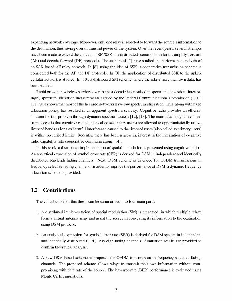
expanding network coverage. Moreover, only one relay is selected to forward the source’s information tothe destination, thus saving overall transmit power of the system. Over the recent years, several attemptshave been made to extend the concept of SM/SSK to a distributed scenario, both for the amplify-forward(AF) and decode-forward (DF) protocols. The authors of [7] have studied the performance analysis ofan SSK-based AF relay network. In [8], using the idea of SSK, a cooperative transmission scheme isconsidered both for the AF and DF protocols. In [9], the application of distributed SSK to the uplinkcellular network is studied. In [10], a distributed SM scheme, where the relays have their own data, hasbeen studied.

Rapid growth in wireless services over the past decade has resulted in spectrum congestion. Interest-ingly, spectrum utilization measurements carried by the Federal Communications Commission (FCC)[11] have shown that most of the licensed networks have low spectrum utilization. This, along with fixedallocation policy, has resulted in an apparent spectrum scarcity. Cognitive radio provides an efficientsolution for this problem through dynamic spectrum access [12], [13]. The main idea in dynamic spec-trum access is that cognitive radios (also called secondary users) are allowed to opportunistically utilizelicensed bands as long as harmful interference caused to the licensed users (also called as primary users)is within prescribed limits. Recently, there has been a growing interest in the integration of cognitiveradio capability into cooperative communications [14].

In this work, a distributed implementation of spatial modulation is presented using cognitive radios.An analytical expression of symbol error rate (SER) is derived for DSM in independent and identicallydistributed Rayleigh fading channels. Next, DSM scheme is extended for OFDM transmissions infrequency selective fading channels. In order to improve the performance of DSM, a dynamic frequencyallocation scheme is provided.

1.2 Contributions

The contributions of this thesis can be summarized into four main parts:

1. A distributed implementation of spatial modulation (SM) is presented, in which multiple relaysform a virtual antenna array and assist the source in conveying its information to the destinationusing DSM protocol.

2. An analytical expression for symbol error rate (SER) is derived for DSM system in independentand identically distributed (i.i.d.) Rayleigh fading channels. Simulation results are provided toconfirm theoretical analysis.

3. A new DSM based scheme is proposed for OFDM transmission in frequency selective fadingchannels. The proposed scheme allows relays to transmit their own information without com-promising with data rate of the source. The bit-error-rate (BER) performance is evaluated usingMonte Carlo simulations.

2

4. DSM implementation is extended to cognitive radio network scenario, where the source, relaysand destination are all cognitive radios. A dynamic frequency allocation scheme is proposed toimprove the performance of DSM. The frequency allocation is modeled through a bipartite graphwith end-to-end symbol error rate (SER) as a weight function. The optimal frequency alloca-tion problem is formulated as minimum weight perfect matching problem and is solved usingthe Hungarian method. Numerical results are provided to illustrate the efficacy of the proposedscheme.

1.3 Structure of the Thesis

To simplify the understanding of this thesis and its contributions, its structure is summarized as fol-lows: Chapter 1 introduces the motivation behind our work. It provides a brief overview of our workand explains its contribution. In Chapter 2, a basic introduction to conventional MIMO system is dis-cussed along with its benefits and shortcomings. In order to facilitate the understanding of DSM, whichis the main focus of this thesis, a brief background to spatial modulation is provided. In addition, a basicintroduction of cooperative relay systems is presented including its advantage, the general architectureand transmission relaying protocols. Moreover, since a cognitive radio system has been selected as anapplication of DSM scheme, the main concept and functions of cognitive radio systems are presented.

In Chapter 3, the proposed DSM scheme for the uplink of cellular network is presented. An analyt-ical expression for symbol error rate (SER) is derived for DSM system in independent and identicallydistributed Rayleigh fading channels. The analytical results are later compared with Monte Carlo simu-lations. Chapter 4 presents the proposed DSM scheme for OFDM transmissions in frequency selectivechannels. The BER performance of DSM-OFDM scheme is evaluated using numerical simulations andcompared with that of distributed Alamouti and direct transmission schemes.

The application of DSM in cognitive radio network is investigated in Chapter 5. A dynamic fre-quency allocation scheme is proposed to allocate unutilized licensed frequencies to secondary sourceand relays. Simulation results are provided to illustrate the efficacy of the proposed scheme. Finally, inthe last chapter which is Chapter 6, this thesis is concluded by summarizing its contributions and alsosuggesting some future possible research directions.

3

Chapter 2

Background and Related Work

This chapter starts with a basic introduction of conventional MIMO systems with their benefits andshortcomings. A brief background of spatial modulation (SM) is provided in Section 2.2 to facilitate theunderstanding of distributed spatial modulation (DSM). A cooperative relay systems with transmissionmodels and relaying protocols are discussed in Section 2.3. Moreover, since a cognitive radio system hasbeen selected as an application of DSM, the main concept and functions of cognitive radio is presentedin Section 2.4.

2.1 Conventional MIMO Systems

With rapid growth in mobile multimedia applications, the demand for higher throughput is expo-nentially increasing in wireless cellular networks. However, available bandwidth below 10 GHz cannotbe scaled at the same rate, which leads to the problem of spectrum scarcity. Multiple Input MultipleOutput (MIMO) transmission has shown the promises to meet the demand for higher throughput. TheMIMO technique is an effective way to increase system capacity and reliability by taking advantagesof spatial multiplexing gain and/or diversity gain, without increasing the use of spectrum. For exam-ple, conventional Bell Labs layered space-time (BLAST) schemes transmit independent data streamssimultaneously over multiple antennas to achieve high multiplexing gain [15]. On the other hand, inspace-time block codes (STBC) technique, multiple copies of a data stream are transmitted over an-tennas and different versions of the data stream received through multiple antennas are then exploitedto achieve maximum diversity gains [16]. Vertical-BLAST (V-BLAST) is the most popular BLASTschemes,which has the simplest detection scheme [17]; whereas Alamouti STBC is the simplest of allSTBC schemes designed for two transmit antennas achieving full diversity gain [18].

The data rate of a MIMO system increases linearly by increasing the number of transmit and receiveantennas. However, several problems are encountered in the development of multiple antenna transmis-sion schemes [19], [20]. These problems arise from several factors, among which are the following.

1. BLAST transmission systems suffer from high inter-channel interference (ICI) at the receiver dueto simultaneous transmissions on the same frequency from multiple antennas.

4

2. The high ICI requires a complex receiver algorithm such as Maximum Likelihood (ML), whichincreases the overall system complexity.

3. Multiple radio frequency (RF) chains are required at the transmitter to be able to transmit manydata streams simultaneously, which do not scale with Moores law and make the transmitter bulky[21].

4. With full-diversity STBC scheme, the above limitations can be overcome. In addition, due to theirorthogonal design, they can easily be decoded at the receiver. However, the maximum spectralefficiency of full diversity STC systems is one symbol per symbol duration for any number oftransmit antennas. Therefore, higher order modulation is required for full-diversity STBC toachieve spectral efficiency same as that of BLAST techniques.

These different problems limit the functionality and applicability of MIMO systems. To overcome theseaforementioned problems, spatial modulation (SM) presents a promising solution and is discussed inthe next section.

2.2 Spatial Modulation

Spatial modulation (SM) is a recently developed transmission technique, which uses multiple trans-mit antennas [2], [3]. In SM, an index of transmit antenna is used as an additional source of informationto improve the overall spectral efficiency. A group of any number of information bits is mapped into twoconstellations: a signal constellation based on modulation scheme and a spatial constellation to encodethe index of the transmit antenna. At any time instant, only one transmit antenna is active, whereas othertransmit antennas radiate zero power. This completely avoids inter channel interference at the receiverand relaxes the stringent requirement of synchronization among the transmit antennas. In addition, un-like conventional MIMO system, SM system does not require multiple RF chains at the transmitter. Atthe receiver, a low complexity decoder such as maximum receive ratio combining (MRRC) is used toestimate the index of active transmit antenna, and after which transmitted symbol is estimated. Usingthese two estimates, a spatial demodulator retrieves the group of information bits.

2.2.1 Operating Principle

In the following, the concept of SM is explained with the aid of some simple examples [22]. Wedenote Nt and Nr, as the number of transmit antennas (TAs) and receive antennas (RAs), respectively.The cardinality of the signal constellation diagram is denoted byM . Either PSK or QAM are considered.In general, Nt, Nr, and M can be chosen independently of each other. At the receiver, optimum MLdemodulation is considered. Thus, Nr can be chosen independently of Nt. For ease of exposition, weassume nt = log2(Nt) and m = log2(M) with nt and m being two positive integers. In Fig. 2.1, theSM concept is illustrated for Nt = M = 2, and it is compared to the conventional Spatial Multiplexing(SMX) scheme and the Orthogonal STBC (OSTBC) scheme designed for transmit diversity. In the lattercase, the Alamouti scheme is considered as an example.

5

Figure 2.1: Illustration of three MIMO concepts [22]: (a) Spatial Multiplexing; (b) Transmit Diversity;and (c) SM.

1. In SMX, two PSK/QAM symbols (S1 and S2) are simultaneously transmitted from a pair of TAsin a single channel use. For arbitrary Nt and M , the rate of SMX is RSMX = Nt log2(M) bpcu.

2. In OSTBC, two PSK/QAM symbols (S1 and S2) are first encoded and then simultaneously trans-mitted from a pair of TAs in two channel uses. For arbitrary Nt and M , the rate of OSTBC isROSTBC = Rc log2(M) bpcu, where Rc = NM/Ncu ≤ 1 is the rate of the space-time blockcode and NM is the number of information symbols transmitted in Ncu channel uses. As shownin Fig. 2.1, if the Alamouti code is chosen, then we have Rc = 1.

3. In SM, only one S1 out of the two symbols is explicitly transmitted, while the other symbol S2is implicitly transmitted by determining the index of the active TA in each channel use. In otherwords, in SM-MIMO, the information symbols are modulated onto two information carryingunits: a) one PSK/QAM symbol; and b) a single active TA via an information-driven antenna-switching mechanism. For arbitrary Nt and M , the rate of SM is RSM = log 2(M) + log 2(Nt)

bpcu.

In Fig. 2.2, the encoding mechanism of SM is illustrated for Nt = M = 4 by considering twogeneric channel uses [23]. The rate of this MIMO setup is RSM = log2(M) + log2(Nt) = 4 bpcu.Therefore, the encoder processes the information bits in blocks of four bits each. In the first channeluse shown in Fig. 2.2(a), the block of bits to be encoded is “1110”. The first log2(Nt) = 2 bits, “11”determine the single active transmit antenna TX3, while the second log2(M) = 2 bits, “10” determinethe transmitted PSK/QAM symbol. Likewise, in the second channel use as shown in Fig. 2.2(b), theblock of bits to be encoded is “0001”. The first log2(Nt) = 2 bits, “00” determine the single activetransmit antenna TX0, while the second log2(M) = 2 bits, “01” determine the transmitted PSK/QAMsymbol.

6

Figure 2.2: Illustration of SM 3-D mapping [23] a) first channel use b) second channel use. The first twoinformation bits define the spatial-constellation point which identifies the active antenna. The remainingtwo bits determine the signal-constellation point that is to be transmitted

The illustrations shown in Fig. 2.2 highlight a pair of unique characteristics of SM.

a) The activated TA may change during every channel use according to the input information bits.Thus, TA switching is an effective way of mapping the information bits to TA indices and ofincreasing the transmission rate.

b) The information bits are modulated onto a 3-D constellation diagram, which generalizes theknown 2-D (complex) signal-constellation diagram of PSK/QAM modulation schemes. The thirddimension is provided by the antenna array, where some of the bits are mapped to the TAs. Thethird dimension is also termed the “spatial-constellation diagram”.

In simple mathematical terms, the signal model of SM, assuming a frequency-flat channel model, isas follows:

y = Hx + n (2.1)

where y ∈ CNr×1 is the complex received vector; H ∈ CNr×Nt is the complex channel matrix; n ∈CNr×1 is the complex AWGN at the receiver; and x = es ∈ CNt×1 is the complex modulated vectorwith s ∈ {s1, s2, . . . , sM} being the complex PSK/QAM modulated symbol belonging to the signal-constellation diagram and e ∈ A being the Nt × 1 vector belonging to the spatial-constellation diagramA as follows:

et =

{1 if the tth TA is active0 if the tth TA is not active

(2.2)

where et is the tth entry of e for t = 1, 2, . . . , Nt. In other words, the points (Nt-dimensional vectors)of the spatial constellation diagram are the Nt unit vectors of the natural basis of the Nt-dimensionalEuclidean space.

7

2.2.2 Maximum Likelihood Receiver

In SM, only one transmit antenna is active at any given time. Therefore, the optimal ML receiver canbe expressed as follows:

[i, s] = arg mini∈{1,...,Nt}s∈{s1,...,sM}

{‖y− his‖2

}

= arg mini∈{1,...,Nt}s∈{s1,...,sM}

{Nr∑d=1

|yd − hi,ds|2} (2.3)

where i and s are estimated antenna index and transmitted symbol. It is applied to SM-demaping toretrieve information bits.

2.2.3 Simulation Results

Fig. 2.3 depicts the symbol error rate (SER) performance of SM over independent and identicallydistributed Rayleigh fading channels. A spectral efficiency of η = 6 and η = 8 bits/s/Hz is achievedusing four transmit antennas (Nt = 4) and 16-QAM (M = 16), and 64-QAM (M = 64) modulationrespectively.

0 5 10 15 20 2510

−5

10−4

10−3

10−2

10−1

100

SNR in dB

SER

SM 8bits 4x4 64QAM Simulation


Figure 2.3: The SER performance of SM is evaluated over independent and identically distributedRayleigh fading channels. The source has four transmit antennas and directly transmits data to the des-tination. A spectral efficiency of 6 and 8 bits/s/Hz is achieved using 16-QAM and 64-QAM modulationrespectively.

8

2.3 Cooperative Relay Network

Unlike traditional point-to-point MIMO systems, a cooperative relay system allows different nodesto share their antennas to form a virtual antenna array. The cooperative relay system can achieve thesame gain benefits of MIMO systems whilst avoiding some of their drawbacks. In fact, it promises sig-nificant improvements in the system reliability and capacity and in service coverage without additionalbandwidth or transmit power.

A cooperative relay system achieves spatial diversity or cooperative diversity by allowing multiplerelays to forward copies of the source’s information in parallel via independent channels with or withoutinformation received from the direct path. This gain comes from the fact that as the number of indepen-dent paths carrying the same information between the source and destination increases, the probabilityof all of them being in fade decreases. This feature provides the ability to overcome the detrimentaleffects of severe fading in the wireless channel. In addition, cooperative relay systems reduces theend-to-end path loss between the source and destination. Since, intermediate relay nodes are placedin between the source and destination, the total resultant pathloss of source-relay and relay-destinationis less than the pathloss of the source-destination. It is known theoretically that the SNR is inverselyproportional to the signal propagation distance, d, as given below:

SNR ∝ 1

dn(2.4)

where d is the distance between the source and destination nodes and n is the pathloss exponent whichtypically fluctuates between 2 and 6 based on the type of the propagation environment.

According to this relation, a cooperative relay system where the intermediate relay is half way be-tween the source and destination and the power is divided equally between the source and the relay willresult in the following gain as compared to the conventional point-to-point system

Gp =

1/2(d/2)n + 1/2

(d/2)n

1dn

= 2n (2.5)

which means the cooperative system can achieve a transmit power saving of (10 log10 2n) dB.The potential advantages offered by cooperative relay systems are mentioned below:• High system reliability: A cooperative relay system can be extremely effective to combat the ef-

fects of channel fading by cooperative diversity. Also, it can effectively enhance the transmissionrobustness by guaranteeing the transmission between the source and destination even if the directlink is in deep fade.• High system coverage: The cooperative relay system can effectively expand the network coverage

through the relaying capability. So, the transmitted signal can travel longer as compared to point-to-point systems. Also, it can expand the network coverage by covering dead holes or spots in thenetwork such as shadowed terminals.• Increasing data rate: The cooperative system can effectively increase the system data rate through

exploiting its multiplexing capability or by exploiting the power gains due to diversity and pathlossgains in increasing the cardinality of the signal constellation.

9

Figure 2.4: A single-relay with direct-link transmission model.

• Interference mitigation: A cooperative relay system can exploit the cooperative diversity to over-come the effects of interference. Also, it can exploit power gains to reduce the required transmitpower which results in alleviating interference. Moreover, it can exploit an appropriate powerallocation to control the transmit power. Furthermore, it can utilize an appropriate relay selectiontechnique to avoid interference.

Next, different relay network architectures and transmission relaying protocols are considered.

2.3.1 Cooperative Relay Network Architecture

A cooperative relay system consists basically of three parts which are the source node, relay nodesand destination node. The source broadcasts its information via one or a number of intermediate re-lays along with the direct source to destination transmission or without it. The destination combinesthe received multiple independent copies of the signal which results in cooperative diversity. So, thenetwork architecture can typically be divided into two models which are a single-relay with direct-linktransmission model and a multiple-relay transmission model. In the following, the two cooperative relaynetwork models are described.

1. A single-relay with direct-link transmission model: In this model, the source node obtains benefitsfrom the available single relay to convey its information to the destination node in addition to thedirect-link between the source and the destination which allows cooperative diversity as shownin Fig. 2.4. This model requires two phases or two hops to complete the whole transmission. Inthe first phase, the source node broadcasts its information to the relay node and to the destinationwhile in the second phase, the relay node relays its received signals to the destination. These twophases should be orthogonal to avoid detrimental interference through transmission.

2. A multiple-relay transmission model: In this model, the source node might send its informationto the destination via a two-hop or multihop protocol with direct-link transmission or without itaccording to the network topology and direct-link transmission availability. So, this model can becategorized as follows:

a) Serial topology with direct-link transmission: In this model, the multiple relays are con-nected in serial and hence the information received from the source should be transferred

10

Figure 2.5: A multiple-relay transmission model (dash line pattern for direct link means it might beavailable or not available). (a) Serial topology with direct-link transmission. (b) Parallel topology. (c)Hybrid topology.

from one another in a multihop transmission to arrive at the destination node in additionto the direct-link transmission as shown in Fig. 2.5(a). The maximum spatial cooperativediversity order which can be attained is two.

b) Parallel topology: In this model, the system consists of parallel paths between the sourceand destination and each path passes through one relay so the transmission through relaynodes requires only two hops as shown in Fig. 2.5(b). This model might include direct-linktransmission or not. This model can offer several features such as a high order cooperativediversity equal to the number of available relay nodes plus one if the direct-link transmissionis available, short-time transmission (only two-hops), ability to exploit the network resourceefficiently, a way to extend the system coverage and a solution to the pathloss and shadowingeffects.

c) Hybrid topology: This model combines between the serial topology and the parallel topol-ogy as shown in Fig. 2.5(c). This model provides increased system complexity and de-creased cooperative diversity as compared with the parallel topology.

2.3.2 Relaying Protocols

Currently, several transmission relaying protocols have been proposed and can be classified accord-ing to their forwarding strategy as:

11

• Amplify-and-Forward (AF): The relay simply amplifies its received signal by a amplificationfactor before forwarding the signal to the destination. In practice, the AF scheme is more attractivedue to its simplicity and low cost implementation since the relay nodes do not need to decode thereceived signals or perform any signal processing. However, in this protocol, the noise is alsoamplified which results in some performance degradation.

• Decode-and-Forward: The relay fully decodes the message from the source, encodes again andtransmits to the destination. Even though, the protocol eliminates the amplification of noise, thedecoding errors can be propagated to the destination that may lead to a wrong decision.

• Estimate-and-forward: These relaying methods are used only when the information from thedirect link is available. The relay does not fully decode the received signal from the source. Itencodes and quantizes a version of the received signal and forwards this extracted informationto the destination. The forwarded information may contain some estimation error. Therefore,this information is used as side information by the destination while decoding the direct linkinformation.

Note that the demodulate-and-forward relaying method is a form of estimate-and-forward methodin which the relay decodes only a fraction of its received signal from the source.

In our work, a parallel topology without direct source-destination path and decode-and-forward re-laying protocol are considered.

2.4 Cognitive Radio

With proliferation in smartphone devices and a growing interest in multimedia applications, there isunprecedented growth in mobile data traffic resulting in problem of spectrum scarcity. Most suitablefrequency bands (below 3GHz) have already been assigned under the licensed bands for the existingwireless systems, which increases the complexity and difficulty to find available frequency bands fornew wireless systems. Furthermore, current spectrum allocation policy is inflexible to allow sharing ofthe licensed bands, although several field measurements performed from leading spectrum regulatorycommissions, such as the Federal Communications Commission (FCC) in the United States [11] veri-fied that there are licensed bands unoccupied most of time or partially occupied. Therefore, there arespectrum holes or white bands in certain time, frequency, and positions as shown in Fig. 5.1, whichresult in reducing the spectrum efficiency.

These challenging problems of spectrum inefficiency motivated researchers to find efficient solutionswhich result in the concept of cognitive radio. It is a new communication paradigm that can effectivelyexploit the existence of spectrum holes by enabling unlicensed users to intelligently utilize these spec-trum holes without causing harmful interference to the licensed users (primary users). Originally, theconcept of cognitive radio is to sense the spectrum in order to find the unoccupied bands and then utilize

12

Figure 2.6: Concept of opportunistic spectrum sharing: secondary utilization of the identified spectrumholes.

them wisely at a certain time [24]. This concept has recently been developed to be fully aware of thesurrounding environment and the primary users, and thereby further improve the efficiency of spectrumutilization.

In particular, the functions of cognitive radio can be categorized into three main functions which arespectrum sensing, spectrum sharing and spectrum management [25]. There are different approachesfor spectrum sensing that have been proposed in the literature [12], [26] and [27]. However, the mostcommon approaches are power energy detection, matched filtering detection, spectrum estimation andcyclostationary feature detection. On the other hand, there are three main spectrum sharing approacheswhich are underlay, overlay and interweave cognitive approaches [28]. In an underlay approach, cog-nitive users are allowed to access the spectrum at any time if the interference caused to primary usersis below an acceptable limit. In an overlay approach, cognitive users forward the primary users trafficin addition to their own traffic provided that they do not cause undue interference to the primary usersthrough exploiting interference cancellation techniques. In an interweave approach, cognitive users areopportunistically accessing the spectrum holes without causing interference to the primary users. Re-cently, there has been a growing interest in the integration of cognitive radio capabilities into cooperativecommunication [14].

In our work, a distributed implementation of spatial modulation (SM) is proposed using cognitiveradios. In distributed spatial modulation (DSM), multiple relays form a virtual antenna array and assist asource to transmit its to a destination. Next, implementation of DSM is extended to a cognitive networkscenario, where the source, relays and destination are all cognitive radios.

13

2.5 Summary

In this chapter, a brief overview of conventional MIMO systems is presented with their benefitsand shortcomings. In addition, to facilitate the understanding of DSM, a brief background of spatialmodulation and cooperative relay system are provided. Moreover, since a cognitive radio system hasbeen selected as an application of DSM, the main concept and functions of cognitive radio is presented.

14

Chapter 3

Distributed Spatial Modulation

Spatial modulation (SM) is a new transmission technique for low-complexity implementation ofMIMO systems. In SM, the index of the active transmit antenna is employed as an additional meansof conveying information. Since, only one transmit antenna is active at any time instant, inter-channelinterference (ICI) and inter-antenna synchronization (IAS) are efficiently avoided. Recent studies [4]-[5] have shown that SM can outperform other state-of-the-art MIMO schemes in terms of computationalcomplexity if many antennas are available at the transmitter. Unfortunately, this makes SM useful onlyin the downlink of the cellular network, where a base station can be equipped with a large number ofantennas. On the other hand, use of multiple antennas in mobile terminals has practical limitations.Besides constraints on complexity and cost, decreasing terminal size restricts the application of SM inthe uplink of cellular network.

To overcome these problems, distributed spatial modulation (DSM) presents a promising solution,where a set of neighboring mobile terminals assist the source in conveying its information to the des-tination [6]. The key idea behind DSM is that multiple cooperative relays share their antennas to forma virtual antenna array (VAA) and apply SM principle in a distributed manner. The DSM system over-comes the limitations of heavy shadowing effects while expanding network coverage. Moreover, onlyone relay is selected to forward the source’s information to the destination, thus saving overall transmitpower of the system. Over the recent years, several attempts have been made to extend the concept ofSM/SSK to a distributed scenario, both for the amplify-forward (AF) and decode-forward (DF) proto-cols. The authors of [7] has studied the performance analysis of a SSK-based AF relay network. In[8], using the idea of SSK, a cooperative transmission scheme is considered both for the AF and DFprotocols. In [9], the application of distributed SSK to the uplink cellular network is studied. In [10], adistributed SM scheme, where the relays have their own data, has been studied.

In this chapter, we focus our attention on application of DSM in the uplink of cognitive relay network.In Section 3.1, we present a system model for DSM based cognitive relay network. This is followedby derivation of analytical SER of DSM in Section 3.2. Section 3.3 presents theoretical and simulationresults.

15

Figure 3.1: DSM system model including one single-antenna source , K single-antenna relays andthe destination with D receive antennas. The source broadcasts its signal (x), which is independentlydemodulated by each relay. Each of the relay then divides the received data (br) in two parts, first part(ur) is used to decide which one of the relays will be active and other part (vr) decides what data it willtransmit to the destination. The received signal at the destination is applied to optimum ML-detectorto determine the estimated index of the active relay (r) and transmitted symbol (z) by the active relay.Information bits are retrieved from these estimates by using DSM mapping table.

3.1 System Model and Notations

We consider a CR network topology with one single-antenna source (S), K single-antenna relays(Rr, with r = 1, 2, ...,K) and a destination (D) with multiple receive antennas, as depicted in Fig. 3.1.This network topology emulates the uplink of the cognitive cellular network, where the source and relaysare secondary users and the destination is cognitive base station. The source and relays opportunisti-cally access licensed spectrum band based on the interweave cognitive radio approach. The followingassumptions are made: a) All nodes operate in half duplex mode. b) The coverage of the source extendsto include relays, but not the destination due to deep fading, heavy path loss or shadowing effects. Itmeans no direct path exists between the source and destination and therefore, relays assist the sourcein transmitting its information to the destination using DSM protocol. c) Relays are either dedicatednetwork elements or idle users, which do not have data to transmit. d) A lexicographic labeling IDRr isused to assign a unique digital identifier to each relay. For example, for K = 4, relays R1, R2, R3 andR4 will have digital identifiers IDR1 = 00, IDR2 = 01, IDR3 = 10 and IDR4 = 11 respectively each oflog2(K) bits.

The whole transmission occurs in two phases and lasts for two time slots i) Broadcasting phase(i.e. first time slot), in which the source broadcasts its information to relays. The source is assumed totransmit either Phase Shift Keying (PSK) or Quadrature Amplitude Modulation (QAM) symbols withconstellation size M . The received signal is demodulated at each relay independently. ii) Relaying

16

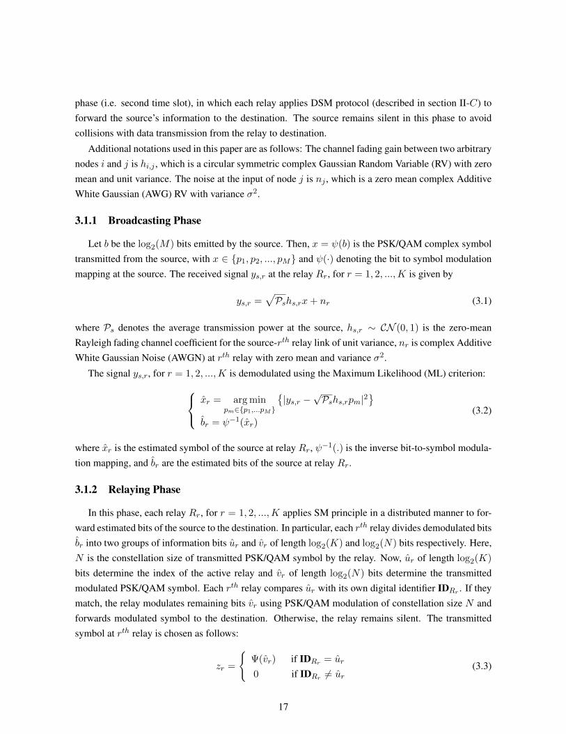
phase (i.e. second time slot), in which each relay applies DSM protocol (described in section II-C) toforward the source’s information to the destination. The source remains silent in this phase to avoidcollisions with data transmission from the relay to destination.

Additional notations used in this paper are as follows: The channel fading gain between two arbitrarynodes i and j is hi,j , which is a circular symmetric complex Gaussian Random Variable (RV) with zeromean and unit variance. The noise at the input of node j is nj , which is a zero mean complex AdditiveWhite Gaussian (AWG) RV with variance σ2.

3.1.1 Broadcasting Phase

Let b be the log2(M) bits emitted by the source. Then, x = ψ(b) is the PSK/QAM complex symboltransmitted from the source, with x ∈ {p1, p2, ..., pM} and ψ(·) denoting the bit to symbol modulationmapping at the source. The received signal ys,r at the relay Rr, for r = 1, 2, ...,K is given by

ys,r =√Pshs,rx+ nr (3.1)

where Ps denotes the average transmission power at the source, hs,r ∼ CN (0, 1) is the zero-meanRayleigh fading channel coefficient for the source-rth relay link of unit variance, nr is complex AdditiveWhite Gaussian Noise (AWGN) at rth relay with zero mean and variance σ2.

The signal ys,r, for r = 1, 2, ...,K is demodulated using the Maximum Likelihood (ML) criterion: xr = arg minpm∈{p1,...pM}

{|ys,r −

√Pshs,rpm|2

}br = ψ−1(xr)

(3.2)

where xr is the estimated symbol of the source at relay Rr, ψ−1(.) is the inverse bit-to-symbol modula-tion mapping, and br are the estimated bits of the source at relay Rr.

3.1.2 Relaying Phase

In this phase, each relay Rr, for r = 1, 2, ...,K applies SM principle in a distributed manner to for-ward estimated bits of the source to the destination. In particular, each rth relay divides demodulated bitsbr into two groups of information bits ur and vr of length log2(K) and log2(N) bits respectively. Here,N is the constellation size of transmitted PSK/QAM symbol by the relay. Now, ur of length log2(K)

bits determine the index of the active relay and vr of length log2(N) bits determine the transmittedmodulated PSK/QAM symbol. Each rth relay compares ur with its own digital identifier IDRr . If theymatch, the relay modulates remaining bits vr using PSK/QAM modulation of constellation size N andforwards modulated symbol to the destination. Otherwise, the relay remains silent. The transmittedsymbol at rth relay is chosen as follows:

zr =

{Ψ(vr) if IDRr = ur

0 if IDRr 6= ur(3.3)

17

Figure 3.2: Illustration of Distributed Spatial Modulation (DSM) with M = 16, N = 4 & K = 4 in theabsence of demodulation errors at relays. A source broadcasts 16-QAM modulated symbol to all relays.Each relay independently demodulate the received signal and divides demodulated bits into two blocks.First log2(K) = 2 bits “01” determine the active relay (R2) and log2(N) = 2 bits “10” determine thetransmitted PSK/QAM symbol.

where, Ψ(.) is bit to symbol mapping at each relay; Ψ(vr) ∈ {q1, q2, ..., qN} is the PSK/QAM complexsymbol transmitted from the relay (when active).

To illustrate, consider an example with K = 4, M = 16 and N = 4. Each relay is assigned aunique digital identifier as follows, IDR1 = 00, IDR2 = 01, IDR3 = 10 and IDR4 = 11. The emittedinformation bits are processed in a block of log2(M) = log2(K) + log2(N) = 4 bits. As shown inthe Fig. 3.2, the source modulates incoming bits {0110} using 16-QAM modulation and broadcastsmodulated symbol to all four relays. Each relay demodulates the received signal independently. Later,demodulated bits are divided into two groups ur and vr of length log2(K) = 2 and log2(N) = 2

bits respectively. In order to simplify the explanation, we assume that there are demodulation errors atrelays. Each relay compares first two bits, i.e. ur with its own digital identifier IDRr . For this specificexample, u2 = {01} matches with digital identifier of R2 (IDR2 = {01}) and therefore, R2 modulatesremaining two bits v2 = {10} using QPSK/4-QAM modulation and forwards modulated symbol to thedestination. In the case ofR1, R3 andR4, ur, for r = 1, 3 and 4 does not coincide with their own digitalidentifier and therefore, these relays remain silent in the relaying phase.

The received signal yd at dth receive antenna of the destination can be expressed as follows:

yd =

K∑r=1

(√Prhr,d zr + nd

)(3.4)

where Pr denotes the average transmission power at each relay, hr,d ∼ CN (0, 1) is the zero-mean andunit variance Rayleigh fading channel coefficient of the link between rth relay and dth receive antenna

18

Table 3.1: DSM Mapping Table: 4 bits/symbol

InputBits

ActiveRelay

TransmitSymbol

0000 1 +1+j0001 1 -1+j0010 1 -1-j0011 1 +1-j0100 2 +1+j0101 2 -1+j0110 2 -1-j0111 2 +1-j1000 3 +1+j1001 3 -1+j1010 3 -1-j1011 3 -1+j1100 4 +1+j1101 4 -1+j1110 4 -1-j1111 4 +1-j

of the destination, nd is complex additive white Gaussian noise (AWGN) at dth receive antenna of thedestination with zero mean and variance σ2.

Assuming that perfect channel state information are available at the receiver, the ML-optimum de-coding rule of DSM can be given as:

(r, z) = arg minr∈{1,...,K}

qn∈{q1,...,qN}

{L∑d=1

|yd −√Prhr,dqn|2

}(3.5)

where L is the number of receive antennas at the destination, r is the estimated index of the active relayand z is the estimated symbol transmitted by the active relay.

Using these estimates, information bits are retrieved by using DSM mapping table shown in Table 3.1.

3.2 Analytical SER Calculation of DSM

In this section, an analytical expression for symbol error ratio (SER) is derived for DSM in inde-pendent and identically distributed (i.i.d.) Rayleigh fading channels. A computation of analytical SERinvolves mainly two estimation processes a) estimation of the index of an active relay, and b) estimationof the transmitted PSK/QAM symbol from the active relay. However, since each relay demodulatesthe received signal independently, some relays demodulate the received signal correctly, whereas someothers may not. This may cause active relays to remain silent, or activate relays which must be silent.

19

Therefore, we must take into account the demodulation errors at relays while computing the SER ofDSM.

To derive the symbol error probability Pe, let Pa denote the probability of incorrect estimation of theindex of the active relay, and let Pd be the probability of incorrect estimation of the transmitted symbolat the destination. In addition, let Pr, (r = 1, 2, ...,K) be the probability of incorrect estimation of thetransmitted symbol at rth relay. The probability of correct estimation of transmitted symbols at all therelays (PcR) can be computed as below:

PcR =

K∏r=1

(1− Pr); (3.6)

However, correct information bits are retrieved at the destination for no demodulation errors at relaysand correct estimation of active relay index and transmitted symbol at the destination. The probabilityof that is

Pc = PcR(1− Pa)(1− Pd) (3.7)

Here, we assume that the estimation of index of the active relay and estimation of the transmitted symbolat the destination are two independent processes. However, if the channel paths are correlated, these twoestimation processes will be dependent. In such a case, the SER expression is an upper bound of thetrue performance in correlated channel conditions. The probability of symbol error is

Pe = 1− Pc (3.8)

In the following subsections, we derive the SER of each estimation process separately

3.2.1 Analytical SER for incorrect estimation of the transmitted symbol

In the relaying phase of DSM, each relay independently demodulates the received signal from thesource. At any time instant, only one relay is active and transmits the modulated symbol of constellationsizeN to the destination, whereas other relays remain silent. Therefore, the estimation of the transmittedsymbol z is the same as a 1 × L MRC detection, where L is the number of receive antennas at thedestination. The average SER of a square QAM signal over Rayleigh fading channels is [29]

Pd = P (z 6= z) = 4q

(1− gd

2

)L L−1∑l=0

(L− 1 + l

l

)(1 + gd

2

)L−

4q2

(1

4− gdπ

([π2− arctan gd

] L−1∑l=0

(2ll

)4(1 + kγd)l

−

sin(arctan gd)

L−1∑l=1

l∑i=1

Til(1 + kγd)l

[cos(arctan gd)]2(l−i)+1

))(3.9)

whereq =

(1− 1√

N

)

20

k =3

2(N − 1)

gd =

√kγd

1 + kγd

Til =

(2ll

)(2(l−i)l−i

)4i(2(l − i) + 1)

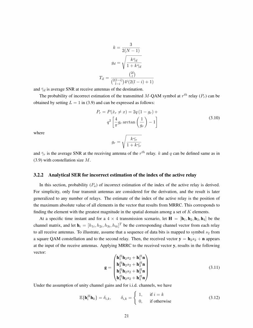
and γd is average SNR at receive antennas of the destination.The probability of incorrect estimation of the transmitted M -QAM symbol at rth relay (Pr) can be

obtained by setting L = 1 in (3.9) and can be expressed as follows:

Pr = P (xr 6= x) = 2q (1− gr) +

q2[

4

πgr arctan

(1

gr

)− 1

] (3.10)

where

gr =

√kγr

1 + kγr

and γr is the average SNR at the receiving antenna of the rth relay. k and q can be defined same as in(3.9) with constellation size M .

3.2.2 Analytical SER for incorrect estimation of the index of the active relay

In this section, probability (Pa) of incorrect estimation of the index of the active relay is derived.For simplicity, only four transmit antennas are considered for the derivation, and the result is latergeneralized to any number of relays. The estimate of the index of the active relay is the position ofthe maximum absolute value of all elements in the vector that results from MRRC. This corresponds tofinding the element with the greatest magnitude in the spatial domain among a set of K elements.

At a specific time instant and for a 4 × 4 transmission scenario, let H = [h1,h2,h3,h4] be thechannel matrix, and let hi = [h1i, h2i, h3i, h4i]

T be the corresponding channel vector from each relayto all receive antennas. To illustrate, assume that a sequence of data bits is mapped to symbol s2 froma square QAM constellation and to the second relay. Then, the received vector y = h2s2 + n appearsat the input of the receive antennas. Applying MRRC to the received vector y, results in the followingvector:

g =

hH1 h2s2 + hH1 nhH2 h2s2 + hH2 nhH3 h2s2 + hH3 nhH4 h2s2 + hH4 n

(3.11)

Under the assumption of unity channel gains and for i.i.d. channels, we have

E{hHi hk} = δi,k, δi,k =

{1, if i = k

0, if otherwise(3.12)

21

Therefore, if the noise is assumed to be AWGN with zero mean and σ2n variance, then three elements inthe vector g have zero mean and σ2n variance. The other element, i.e., the second element in (3.11), hasmean s2 and variance σ2n. The square QAM signal is decomposed into two independent but identicalamplitude modulated signals: a) in phase I , and b) quadrature phase Q. However, only the real positivepart of the QAM constellation is considered for the calculation. Assume that µi is the absolute value ofthe real part of the transmitted symbol. Then, µ is a vector of length c = 2(m/2)−1, which contains thepositive real part elements of the constellation diagram. Let P (µi) denotes the probability that estimateof the index of the active relay is incorrect when transmitting µi. Then, the average overall probabilityfor incorrect estimation of the active relay index, when considering the real part Par, is given by

Par =1

c

c∑i=1

P (µi) (3.13)

The probability of incorrect estimation of the active relay index for the imaginary part is same as thatof the real part. The probability that the estimation is correct for both real and imaginary parts is theproduct of two probabilities, namely, (1 − Par)(1 − Par). As a result, the overall probability of error,when considering both real and imaginary parts, is given as follows:

Pa = 1− (1− Par)2 = 2Par − (Par)2 (3.14)

Next, we derive the the probability (Par) of incorrect estimation of the active relay. Let x = |v|, wherev is a random variable that follows a Gaussian distribution with mean µi and variance σ2n. Then, theprobability density functions (pdfs) for v and x for each µi are

fV (v|µi, σ2n) =1

σn√

2πexp− (v−µi)

2

2σ2n (3.15)

fX(x|µi, σ2n) =1

σn√

2π

(exp− (x−µi)

2

2σ2n + exp− (x+µi)

2

2σ2n

)(3.16)

The second step in estimating the index of the relay is finding the position of the element in g with amaximum absolute value. This is done by computing the pdfs of the sorted Nt random variables, whereeach has a pdf as given in (3.16), but with different means. This problem can be treated with orderstatistics [30].

Let X(1), ..., X(Nt) denote the order statistics of random samples from a continuous population witha cumulative distribution function FX(x|µi, σ2n) and pdf fX(x|µi, σ2n), whereX(Nt) > X(Nt−1) > ... >

X(1). Then, pdf of X(j) is

fX(j)(x|µi, σ2n) =

n!

(j − 1)!(Nt − j)!fX(x|µi, σ2n)

×[FX(x|µi, σ2n)]j−1 × [1− FX(x|µi, σ2n)]Nt−j(3.17)

Considering the current case of four relays, Fig. 3.3 shows the order statistics pdfs of the four randomvariables, which result from taking the maximum of the absolute value of each element in the vector,

22

0 0.5 1 1.5 2 2.5 30

0.5

1

1.5

2

2.5

3

3.5

4

x

fX(x)

f4(x)

f3(x)

f2(x)

f1(x)

SNR =15 dB64QAM µ1 = 1

0 1 2 3 4 50

0.5

1

1.5

2

2.5

3

3.5

4

4.5

x

fX(x)

f4(x)f3(x)f2(x)f1(x)

SNR=15 dB64QAM µ3 = 5

Figure 3.3: Order statistics pdfs of four random variables. The left figure shows the pdfs at SNR = 15dB for 64 QAM and for µ1 = 1, whereas the right figure shows the same pdfs at the same SNR but withµ3 = 5. The small circles inside the left figure shows the crossing point between the pdfs, whereas thereis no intersection among pdfs in the right figure. It is clearly shown that the error contribution from thesecond maximum is the largest, then from the third maximum, and so on.

which results from MRRC at the receiver. If the order statistics pdfs are assumed to be statisticallyindependent, the probability that the antenna number estimation is incorrect can be found by numericallyintegrating the intersection areas of fX(4)

(x|µi, σ2n) with all other distributions for each mean value.However, the assumption of statistical independence is an approximate, since the pdfs are derived basedon the conditional probability that X(Nt) > X(Nt−1) > ... > X(1). Nevertheless, it will be shown inSection 3.3.1 that both analytical and simulation results demonstrate a very close match, which indicatesthat the previous approximations are valid.

Let x3, x2, and x1 indicate the intersection points (bold circles in Fig. 3.3) between fX(4)(x|µi, σ2n)

and fX(3)(x|0, σ2n), fX(2)

(x|0, σ2n), and fX(1)(x|0, σ2n), respectively. Fig. 3.3 shows that x3 > x2 >

x1 > 0, which indicates that the error contribution from the second largest sample is always the highest,followed by that of the third largest sample, and so on. The probability of error for each µi is, then,given by averaging the multiple hypothesis errors as follows:

P (µi) =1

3

(∫ x3

0fX(4)

(x|µi, σ2n) dx+

∫ x2

0fX(4)

(x|µi, σ2n) dx+

∫ x1

0fX(4)

(x|µi, σ2n) dx

)(3.18)

For any number of relays, (3.18) can be written as

P (µi) =1

Nt − 1

(Nt−1∑i=1

∫ xi

0fX(Nt)

(x|µi, σ2n) dx

)(3.19)

Knowing P (µi) for ∀i, Par is calculated as in (3.13). Par is used to compute Pa as in (3.14). Theprobability of incorrect estimation of transmitted symbol at the destination Pd is calculated using (3.9).Similarly, using (3.10), we can compute the probability of incorrect estimation of transmitted symbol at

23

each relay. By computing Pr ∀r, we can calculate PcR using (3.6). Then, Pa, Pd and PcR are used tocalculate the overall SER Pe as in (3.7).

3.3 Simulation Results

In this section, the symbol error rate (SER) performance of DSM is evaluated using analytical ex-pressions and through Monte Carlo simulations. The SER performance of DSM is also compared withconventional SM under the constraint of same spectral efficiency. In addition, we present numerical plotsshowing the performance gain obtained by using the proposed dynamic frequency allocation scheme.

For all system configurations, the average SNR during the first hop (source-relay) is defined as γsr =

10 log10(Ps/σ2), where Ps is the average transmit power at the source. During the second hop (relay-destination), the average SNR is defined as γrd = 10 log10(Pr/σ2), where Pr is average transmit powerat the relay. In all simulations, the total transmit power PT is kept equal to 1W for fair comparisons.Since, only one relay is active in the relaying phase, the total transmit power is divided between thetransmit power at the source and at the relay i.e., (PT = Ps + Pr). It is assumed that channel stateinformation (CSI) is available at all relays and the destination. All simulations were carried out for 2000frames, where each frame contained 500 symbols.

3.3.1 Analytical SER performance of DSM

Fig. 3.4 shows analytical and simulation results for the SER of DSM over i.i.d. Rayleigh fadingchannels for the spectral efficiency of 6 and 8 bits/s/Hz. A spectral efficiency of 6 bits/s/Hz is achievedby using four relays (K = 4) and 16-QAM (N = 16) constellation size (4 × 4 16-QAM), while 8bits/s/Hz is achieved using four relays (K = 4) and 64-QAM (N = 16) constellation size (4 × 4

64-QAM). The source transmits modulated symbols with constellation size of 64-QAM (M = 64) and256-QAM (M = 256) to all the relays to achieve the spectral efficiency of 6 and 8 bits/s/Hz respectively.In both configurations, four receive antennas (L = 4) are considered at the destination. In addition, equalpower allocation between broadcasting and relaying phase is considered i.e. Ps = 1/2;Pr = 1/2. Asshown in Fig. 3.4, the analytical SER performance match closely with simulation results for wide rangeof SNR.

3.3.2 Performance comparison between DSM and SM

Fig. 3.5 compares the SER performance of DSM with conventional SM under the constraint of samespectral efficiency. In SM, it is assumed that the source has four transmit antennas and directly transmitsdata to the destination by applying SM principle. A spectral efficiency of 6 and 8 bits/s/Hz is achievedby using modulation with constellation size of 16-QAM (M = 16) and 64-QAM (M = 64). For faircomparison, the average transmit power at the source is kept 1W, i.e., Ps = 1. In DSM, four relays(K = 4) are used along with modulation of 16-QAM (N = 16) and 64-QAM (N = 64) constellation to

24

0 5 10 15 20 2510

−5

10−4

10−3

10−2

10−1

100

SNR in dB

SER

DSM 8bits 4x4 64QAM Analytical

DSM 8bits 4x4 64QAM Simulation

DSM 6bits 4x4 16QAM Analytical


Figure 3.4: Analytical and simulation results are compared for 6 and 8 bits/s/Hz spectral efficiencies.A spectral efficiency of 6 bits/s/Hz is achieved by using 4 relays (K = 4) and 16-QAM (N = 16)constellation size (4×4 16-QAM), whereas a spectral efficiency of 8 bits/s/Hz is achieved using 4 relays(K = 4) and 64-QAM (N = 64) constellation size (4 × 4 64-QAM). The analytical and simulationresults are in close agreement for wide range of SNR.

0 5 10 15 20 2510

−5

10−4

10−3

10−2

10−1

100

SNR in dB

SER





Figure 3.5: The SER performance of DSM is compared with conventional SM. In SM, the source is as-sumed to have four transmit antennas and directly transmits data to the destination. A spectral efficiencyof 6 and 8 bits/s/Hz is achieved using 16-QAM and 64-QAM modulation respectively. Simulation re-sults demonstrate the significant improvement in the SER for DSM over conventional SM, where a gainof 2-3 dB can be noticed for SER of 10−4.

25

0 5 10 15 20 2510

−5

10−4

10−3

10−2

10−1

100

SNR in dB

SER

DSM 8bits; Ps=0.5 & Pr=0.5

DSM 8bits; Ps=0.75 & Pr=0.25

DSM 8bits; Ps=0.25 & Pr=0.75

DSM 6bits; Ps=0.5 & Pr=0.5

DSM 6bits; Ps=0.75 & Pr=0.25

DSM 6bits; Ps=0.25 & Pr=0.75

Figure 3.6: The SER performance of DSM is evaluated in different power allocation schemes for 6 and8bits/s/Hz spectral efficiencies. The total transmit power is kept 1W and is divided between the sourceand relay. The following three cases are considered: i) Ps = 1/2;Pr = 1/2; ii) Ps = 3/4;Pr = 1/4;iii) Ps = 1/4;Pr = 3/4. It is observed that allocating more power to the active relay in the relayingphase improves SER performance.

achieve spectral efficiency of 6 and 8 bits/s/Hz respectively. In addition, equal power allocation betweenbroadcasting and relaying phase is considered i.e. Ps = 1/2;Pr = 1/2. In Fig. 3.5, simulation resultsclearly demonstrate the significant enhancements in the SER performance of DSM over conventionalSM, where an improvement of 2-3 dB can be noticed for SER of 10−4.

3.3.3 Performance evaluation of DSM for different power allocations

Fig. 3.6 presents numerical plots of the SER of DSM by varying the power allocated in the broad-casting and relaying phase. All previous simulations were carried out under equal power allocationscheme, where the total transmission power was equally divided between the source and the relay, i.e.Ps = 1/2;Pr = 1/2. In this simulation, we consider following three cases: i) Ps = 1/2;Pr = 1/2;ii) Ps = 3/4;Pr = 1/4; iii) Ps = 1/4;Pr = 3/4.

In Fig. 3.6, it can be observed that allocating more power to the active relay in the relaying phaseimproves the SER performance. From the analytical expression of symbol error probability, it is clearthat the SER of DSM depends on i) estimation of transmitted symbols at relays ii) estimation of indexof the active relay iii) estimation of transmitted symbol at the destination. At lower SNR, errors inthe estimation of transmitted symbol dominate the SER. On the other hand, errors in the estimation ofactive relay dominate the SER at higher SNR. However, the probability of error in incorrect estimationof transmitted symbol decreases rapidly with respect to average SNR as compared to the probability of

26

error in in correct estimation of the active relay index. In the case of Ps = 3/4;Pr = 1/4, averageSNR of the source-relay link is more as compared to that to that of relay-destination link. Therefore,the SER is more dominated by errors in the estimation of active relay index. On the other hand, incase (Ps = 1/4;Pr = 3/4), average SNR of the source-relay link is less as compared to that of therelay-destination link. Therefore, the SER is more dominated by errors in the estimation of transmittedsymbols at relays. However, for the same SNR value, errors in the estimation of transmitted symbol ismuch less as compared to estimation errors of the active relay.

3.4 Summary

In this chapter, we presented a distributed implementation of spatial modulation for the uplink ofcellular network. An analytical expression for symbol error probability is derived for DSM in i.i.d.Rayleigh fading channels. Tha analytical results are shown to be in a close agreement with simulationresults for a wide rang of SNR. In addition, the SER performance is compared with conventional SM,where a performance gain of 2-3 dB is noticed in DSM at SER of 10−4

27

Chapter 4

Distributed Spatial Modulation-OFDM

Spatial Modulation(SM) [2], [3] is recently developed MIMO, in which the index of the transmitantenna along with the signal constellation is exploited to convey the information bits. Since, only onetransmit antenna is active at any instance of time, SM completely avoids inter-channel interference andinter-antenna synchronization. Unlike conventional MIMO, SM does not require multiple RF chainsat the transmitter, which makes it energy efficient technique. However, SM is intended for flat fadingchannels and is not suitable for broadband wireless channels, which are frequency-selective. Thank-fully, orthogonal frequency division multiplexing (OFDM) converts a frequency-selective channel intomultiple narrowband flat-fading channels. Therefore, a combination of SM with OFDM is an attractivesolution for next generation broadband wireless communication. SM-OFDM was first proposed in [31]for flat-fading channel and further studied in [32] for multipath fading channels. The effect of channelimperfections on SM-OFDM was investigated in [33], whereas the performance of SM-OFDM in LTEbased system was evaluated in [34].

Recent studies [4], [5] have shown that SM can outperform other state-of-the-art MIMO schemes interms of computational complexity, if many antennas are available at the transmitter. The same resultsare applicable to SM-OFDM, which makes it useful only in the downlink of cellular networks. However,it may be difficult to exploit SM-OFDM in the uplink of cellular network with current technology.Fortunately, through relaying and cooperation, multiple mobile terminals can be grouped together toform a virtual antenna array (VAA), which can be exploited to use SM-OFDM in a distributed manner inthe uplink of cellular systems. However, the relaying has some design problems, such that relays need tohold back their own transmission as well as they need to spend their own resources at the expenses of thesource’s transmission. Motivated by these considerations, we propose a new DSM scheme for OFDMtransmission in a relay-assisted cellular network. Unlike in conventional relay system, the proposedscheme allows relays to transmit their own data traffic, without compromising with the sources datarate. Furthermore, via Monte-Carlo simulations it is shown that the proposed scheme outperforms thedirect transmission OFDM and distributed Alamouti-coded OFDM scheme for higher data rate.

28

4.1 System Model and Notations

The system model is presented in Fig. 4.1. A wireless network topology with a single-antennasource (S), K single antenna relays (Rr with r = 1, 2, ...,K) and a destination (D) with multiple receiveantennas is considered. The following assumptions are made: a) All nodes operate in half-duplex mode.b) The coverage of the source extends to include relays, but not the destination due to deep fading,heavy path or shadowing effect. It means no direct path exists between the source and destination. c)A lexicographic labeling IDRr is used to assign an unique digital identifier to each relay. For example,for K = 4, relays R1, R2, R3, R4 will have digital identifiers IDR1 = 00, IDR2 = 01, IDR3 = 10, andIDR4 = 11 respectively each of length log2(K) bits.

The whole transmission occurs in two phases and lasts for two time slots 1) broadcasting phase(first time slot) in which the source broadcasts its information to all the relays. The source appliesincoming binary data to OFDM modulator and broadcasts the resulting OFDM signal over multipathRayleigh fading channels between the source and relays. Each of the relays independently demodulatesthe received OFDM signal using OFDM demodulator 2) relaying phase (second time slot) in whichrelays use DSM-OFDM protocol (described in the next section) to forward the sources information tothe destination. The source remains silent during this phase to avoid collisions with data transmittedfrom relays to the destination. Using DSM-OFDM protocol, each relay encodes demodulated binarydata such that in each OFDM subcarrier, only one relay transmits the data, while other relays radiatezero power. The number of subcarriers required to transmit the source’s information depends on thenumber of available relays and modulation schemes used both at the source and relays. It is possiblethat all the subcarriers are not required to forward the source’s information. Therefore, the remainingsubcarriers can be utilized by the relays to transmit their own information.

It is assumed that the channel state information (CSI) is not available at the transmitter, but perfectlyknown at the destination and all the relays. The multipath Rayleigh fading channel matrix between Nt

transmit and Nr receive antennas is given below:

H(t) =

h1,1(t) h1,2(t) . . . h1,Nt(t)

h2,1(t) h2,2(t) . . . h2,Nt(t)...

.... . .

...hNr,1(t) hNr,2(t) . . . hNr,Nt(t)

(4.1)

hi,j(t) is a channel vector of size ρ× 1 between jth transmit antenna and ith receive antenna containingall the multipath channel gains and can be written as follows:

hi,j(t) =[h1i,j(t) h2i,j(t) . . . hρi,j(t)

]T(4.2)

29

Figure 4.1: DSM-OFDM system model including one single-antenna source, K single-antenna relaysand the destination with L receive antennas. The source broadcasts OFDM signal s(t), which is inde-pendently demodulated by each relay using OFDM demodulator. Using DSM-OFDM protocol, eachrelay encodes demodulated binary data such that in each OFDM subcarrier, only one relay transmits thedata, while other relays radiate zero power.

4.1.1 Broadcasting Phase

Let b be the log2(M) bits emitted by the source. The source maps b to a binary matrix Q(k) ofsize m × NFFT , where m = log2(M) is the number of bits/symbol per subcarrier and NFFT is thenumber of OFDM subcarriers. Now, m bits of each column of matrix Q(k) are modulated using QAMmodulation of constellation size M . The resulting vector x(k) = [X(0), X(1), . . . , X(NFFT − 1)] ofsize 1×NFFT is applied to OFDM modulator to get a complex baseband time domain signal s(t).

s(t) =1√NFFT

NFFT−1∑k=0

X(k) expj2πtkNFFT ; 0 ≤ t ≤ NFFT − 1 (4.3)

30

The source broadcasts the OFDM signal s(t) over multipath Rayleigh fading channels between thesource and relays, having channel matrix HR,S(t) of size K × 1. Each element hr,s of the matrix HR,S

is a vector of length ρ, where ρ is the number of channel paths between the source and rth relay. Eachrelay independently demodulates the received OFDM signal ys,r(t), for r = 1, 2, . . . ,K using OFDMdemodulator.

4.1.2 Relaying Phase

In this phase, each relay Rr, for r = 1, 2, . . . , ,K applies DSM-OFDM principle to forward thesource’s information to destination. Each rth relay maps demodulated binary data vector bbbr into anotherfrequency vector cr(k) = [Cr(0), Cr(1), . . . , Cr(NFFT − 1)] of size 1×NFFT . In particular, a binarydata vector bbbr for each relay is first mapped to a matrix Wr(k) of size n×Nsub. Here, n = log2(N) +

log2(K) is the number of bits/symbol per subcarrier, which are transmitted in one OFDM block by eachrelay;N is the size of QAM constellation andNsub = NFFT

(n/m) is the number of subcarriers required by therelay to forward the source’s information. Now, n bits of each column of the matrix Wr(k) are dividedinto two group of information bits ur(k) and vr(k) of length log2(K) and log2(N) bits respectively.For each kth subcarrier, ur(k) is compared with unique digital identifier of the rth relay IDRr . If theymatch, the relay modulates remaining vr(k) bits of the corresponding column of the matrix Wr(k) usingQAM modulation of constellation size N . Otherwise, zero power is transmitted in the correspondingsubcarrier.

Cr(k) =

{Ψ(vr(k)) if IDRr = ur(k)

0 if IDRr 6= ur(k)for k = 0, 1, . . . , Nsub − 1 (4.4)

where ur(k) is log2(K) bits of column of the matrix Wr(k) and vr(k) are remaining bits which aremodulated using QAM modulation function Ψ(.) of constellation size N .

Out of NFFT subcarriers, only Nsub subcarriers are utilized in one OFDM block by each relay toforward the sources information. The remaining subcarriers (NFFT −Nsub) are equally distributedamong all the relays to transmit their own information. Each relay inserts its modulated data on theallocated subcarriers. The resultant vector cr(k) is then applied to OFDM modulator to get complexbaseband time domain signal zr(t).

zr(t) =1√NFFT

NFFT−1∑k=0

Cr(k) expj2πtkNFFT ; 0 ≤ t ≤ NFFT − 1 (4.5)

Now, each relay simultaneously transmit complex baseband time domain signal zr(t) over multipathRayleigh fading channels having channel matrix HD,R(t), where each element hd,r(t) is a channelvector of length ρ between rth relay and dth receiving antenna of the destination, where ρ is the numberof multipaths.

31

Figure 4.2: Illustration of DSM-OFDM for 2 bits/symbol/subcarrier transmission, with K = 2 andNFFT = 8. Each relay independently demodulates the received signal and maps demodulated bitsinto a matrix Wr(k) of size n × Nsub. Now, log2(K) = 1 bits of each column of the matrix Wr(k)are compared with digital identifier IDRr of the relay. If they match, remaining bits of that columnare modulated using N -QAM modulation, else zero power is transmitted in that subcarrier. Remainingsubcarriers are equally distributed among relays to transmit their own information.

To illustrate, consider an example of DSM-OFDM with number of relays K = 2 and number ofsubcarriersNFFT = 8. Incoming binary data is mapped to matrix Q(k) of size 1×8,m = log2(M) = 1

and M = 2, for BPSK modulation. Now, 1 bit of each subcarrier is modulated using BPSK modulationto get a vector x(k) of size 1× 8, which is applied to OFDM modulator to get OFDM signal s(t). Thesource broadcasts OFDM signal over a fading channel HR,S . Now, each relay individually demodulatesthe received signal. At rth relay, demodulated binary data vector bbbr is mapped to cr(k) of size 1×8 usingDSM-OFDM principle. In Fig. 4.2, distributed SM-OFDM mapping is illustrated for the transmissionof 2 bits/symbol/subcarrier. It is assumed that two relays (K = 2) demodulate the data without error.Demodulated data sequence bbbr is mapped to Wr(k) of size n × Nsub. For this example, for BPSKmodulation (N = 2) at relay, n = log2(2) + log2(2) = 2 and number of subcarriers allocated toforward sources information is Nsub = NFFT

(n/m) = 8/(2/1) = 4. Now, for rth relay, if log2(K) = 1 bit ofeach column of Wr(k) matches with digital identifier of rth relay (IDR1 = 0 and IDR2 = 1), remaininglog2(N) = 1 bit will be modulated using BPSK modulation and transmitted in that subcarrier, elsezero power will be transmitted. The remaining four subcarriers (NFFT − Nsub = 4) can be allocatedequally among relays to transmit their own information. Each relay transmits modulated symbols in theallocated subcarriers. In this example, subcarriers 5 and 6 are assigned to relay R1 , whereas subcarriers7 and 8 are assigned to relay R2 to transmit their information. Both relays R1 and R2 transmits QPSKmodulated symbols in their allocated subcarriers.

32

4.1.3 Demodulation and Relay Data Extraction

At the destination, the received signal yd(t) at dth antenna is demodulated using OFDM demodulatorresulting in the matrix Y(k) of size L × NFFT , where L is the number of receive antennas at thedestination. Each column vector of Y(k) contains the received data for each subcarrier. For slowlyvarying channel, the received signal which is demodulated using NFFT units, can be expressed as

Yd(k) =K∑r=1

Hd,r(k)Cr(k) + nd(k) (4.6)

where, Hd,r(k) is the frequency response of the subcarrier between the dth receive antenna of the desti-nation and transmit antenna of the rth relay; Yd(k) denotes the demodulated received symbol at the kth

subcarrier of the dth antenna.The transmitted frequency signal cr(k) of each relay Rr for r = 1, 2, . . . ,K can be represented in

the matrix form as below:

C =

C1(0) C1(1) . . . C1(NFFT − 1)

C2(0) C2(1) . . . C2(NFFT − 1)...

.... . .

...CK(0) CK(1) . . . CK(NFFT − 1)

(4.7)

Accordingly, (4.7) is modified as below:

y(k) = H(k)c(k) + n(k) (4.8)

where H(k) = {Hd,r(k)} is the L×K discrete time invariant frequency response channel matrix, c(k)

is the kth column of matrix C, and n(k) is the kth column of the noise matrix n.Here, it is required to determine the index of the active relay and the transmitted symbol from the

active relay. For the detection of relay index and symbol, we have used joint ML detection as proposedin [4]. Assume that CSI is perfectly known at the destination, given a received signal, ML algorithmde-maps it as below:

[r, s] = arg minr∈{1,...,K}s∈{s1,...,sM}

Py(y(k)|c(k),H(k))

= arg minr∈{1,...,K}s∈{s1,...,sM}

{‖y(k)−H(k)c(k)‖2F

}for k = 0, 1, . . . , Nsub − 1

(4.9)

where r denotes the estimated index of the active relay and s denotes the estimated transmitted symbol.Given a received signal y(k), the ML decodes this as symbol sequence which maximizes the likelihoodfunction Py(y(k)|c(k),H(k)) that y(k) is received given that c(k) was transmitted. Later, DSM-OFDMde-mapping table is used to retrieve the sources information, which is present in the first Nsub subcarri-ers. For example, for 2 bits/symbol/subcarrier transmission, if estimated relay index is 2 and estimatedsymbol is −1 (BPSK symbol), the sources information bits are {10} as shown in the table of Fig. 4.2.

33

Table 4.1: Simulation Parameters

Parameters ValueCarrier Frequency 2 GHz

Bandwidth 20 MHzSubcarrier Spacing 15 KHz

Length of cyclic prefix 32Relay Schemes 2× 4, 4× 4, and 8× 4

Channel Estimation IdealModulation Schemes QAM

Maximum Doppler Shift 6 HzChannel Model Rayleigh Frequency Selective Fading

From remaining subcarriers, the relay’s information is extracted using ML algorithm as below:

[s] = arg mins∈{s1,...,sM}

{‖y(k)−H(k)c(k)‖2F

}for k = Nsub, . . . , NFFT − 1 (4.10)


In this section, the bit error ratio (BER) performance of DSM-OFDM scheme is evaluated usingMonte Carlo simulations. The multipath Rayleigh fading channel model is considered and its parametersare summarized in Table 4.1. It is assumed that channel state information (CSI) is available at thedestination and all the relays. For a fair comparison, the total transmission power in each subcarrier isset to 1W for all the schemes and it is equally divided between the broadcasting and relaying phase.Perfect frequency and time synchronization is assumed.

Fig. 4.3 and 4.4 compare the BER performance of DSM-OFDM with distributed Alamouti-OFDMand direct transmission-OFDM (DT-OFDM) scheme under the constraint of same spectral efficiency.The distributed Alamouti-OFDM schemes is proposed in [35]. Each of the relays independently de-modulates the received signal and encodes data according to Alamouti SFBC scheme in two subsequentsubcarriers of the OFDM symbol. All the relays simultaneously transmit OFDM signal to the destina-tion. At the destination, a low complexity optimal decoder is applied for each two subcarriers to retrievethe source’s information. In DT-OFDM, the source directly transmits OFDM signal to the destination,without involving relays.

4.2.1 Four bits transmission

Fig. 4.3 shows the BER performance of DSM-OFDM for 4 bits/symbol/subcarrier spectral efficiency.It can be achieved by two configurations. The first configuration (2 × 4 16-QAM) uses two relays(K = 2) with 16-QAM (N = 16) modulation, whereas the second configuration (4 × 4 8-QAM) usesfour relays (K = 4) with 8-QAM (N = 8) modulation. In both configurations, four receive antennas(L = 4) are considered at the destination. In addition, we assume that the relays simultaneously transmit

34

0 5 10 15 20 2510

−5

10−4

10−3

10−2

10−1

100

SNR in dB

BER

DSM−OFDM 2x4 16QAM

DSM−OFDM 4x4 8QAM

Alamouti−OFDM 2x4 16QAM

DT−OFDM 16QAM

Figure 4.3: The BER performance of DSM-OFDM scheme is compared with distributed Alamouti-OFDM and DT-OFDM for spectral efficiency of 4 bits/symbol/subcarrier. The 2×4 16-QAM distributedAlamouti-OFDM configuration outperforms all other schemes. The 2× 4 16-QAM DSM-OFDM con-figuration shows degraded performance as compared to 4 × 4 8-QAM for low SNR (SNR < 15 dB),but it shows better performance for higher SNR (SNR > 15 dB). The DT-OFDM shows worst BERperformance.

their own data in the available subcarriers in both the configurations. Moreover, a 2 × 4 16-QAMdistributed Alamouti-OFDM configuration transmits the same number of information bits per subcarrier.In DT-OFDM, the source uses 16-QAM (M = 16) modulation scheme in each subcarrier of the OFDMsymbol and directly transmits to the destination.

The 2 × 4 16-QAM distributed Alamouti-OFDM configuration outperforms all other schemes. Fora low spectral efficiency, diversity gain of Alamouti scheme dominates the BER performance. The2× 4 16-QAM DSM-OFDM configuration shows degraded performance as compared to 4× 4 8-QAMfor low SNR (SNR < 15 dB), but it shows better performance for higher SNR (SNR > 15 dB). Thiscan be explained by the fact that for low SNR, the error is dominated by incorrect estimation of thetransmitted symbol, whereas for higher SNR, it is dominated by incorrect estimation of index of theactive relay. The DT-OFDM shows worst BER performance. Relays transmit their own information inthe allocated subcarriers and data rate achieved by the relays depend on number of free subcarriers andmodulation scheme used at relays.

4.2.2 Six bits transmission

Fig. 4.4 shows the BER performance of 4 × 4 32-QAM and 8 × 4 16-QAM DSM-OFDM con-figurations. The BER performance is compared with 2 × 4 64-QAM distributed Alamouti-OFDM and64-QAM DT-OFDM schemes for the same spectral efficiency of 6 bits/symbol/subcarrier. The first con-

35

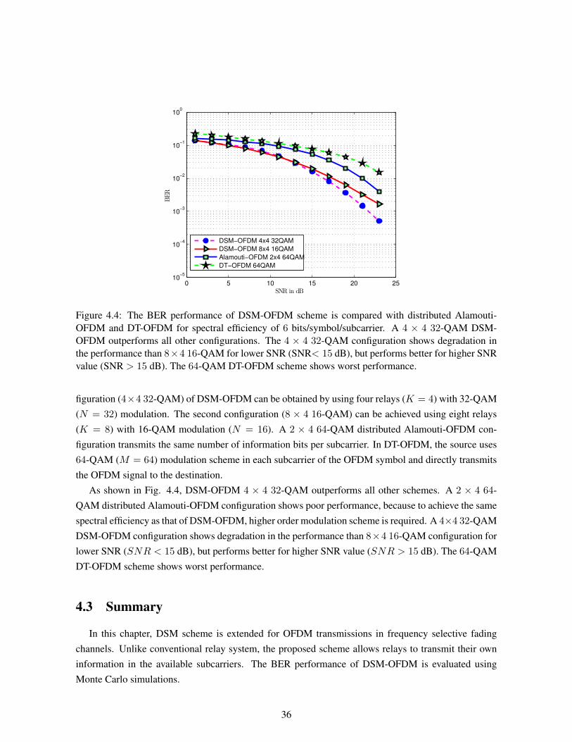
0 5 10 15 20 2510

−5

10−4

10−3

10−2

10−1

100

SNR in dB

BER



Alamouti−OFDM 2x4 64QAM

DT−OFDM 64QAM

Figure 4.4: The BER performance of DSM-OFDM scheme is compared with distributed Alamouti-OFDM and DT-OFDM for spectral efficiency of 6 bits/symbol/subcarrier. A 4 × 4 32-QAM DSM-OFDM outperforms all other configurations. The 4 × 4 32-QAM configuration shows degradation inthe performance than 8×4 16-QAM for lower SNR (SNR< 15 dB), but performs better for higher SNRvalue (SNR > 15 dB). The 64-QAM DT-OFDM scheme shows worst performance.

figuration (4×4 32-QAM) of DSM-OFDM can be obtained by using four relays (K = 4) with 32-QAM(N = 32) modulation. The second configuration (8 × 4 16-QAM) can be achieved using eight relays(K = 8) with 16-QAM modulation (N = 16). A 2 × 4 64-QAM distributed Alamouti-OFDM con-figuration transmits the same number of information bits per subcarrier. In DT-OFDM, the source uses64-QAM (M = 64) modulation scheme in each subcarrier of the OFDM symbol and directly transmitsthe OFDM signal to the destination.

As shown in Fig. 4.4, DSM-OFDM 4 × 4 32-QAM outperforms all other schemes. A 2 × 4 64-QAM distributed Alamouti-OFDM configuration shows poor performance, because to achieve the samespectral efficiency as that of DSM-OFDM, higher order modulation scheme is required. A 4×4 32-QAMDSM-OFDM configuration shows degradation in the performance than 8×4 16-QAM configuration forlower SNR (SNR < 15 dB), but performs better for higher SNR value (SNR > 15 dB). The 64-QAMDT-OFDM scheme shows worst performance.

4.3 Summary

In this chapter, DSM scheme is extended for OFDM transmissions in frequency selective fadingchannels. Unlike conventional relay system, the proposed scheme allows relays to transmit their owninformation in the available subcarriers. The BER performance of DSM-OFDM is evaluated usingMonte Carlo simulations.

36

Chapter 5

Dynamic Frequency Allocation for DSM based Cognitive Radio Network

In this chapter, the implementation of DSM is extended to cognitive network scenario, where asource, relays and destination are all cognitive radios. A dynamic frequency allocation scheme is pro-posed to improve the performance of DSM in this scenario. Section 5.1 presents a system model forDSM based cognitive relay network. A dynamic frequency allocation schemes for the source and relaysare described in Section 5.2. Numerical results are provided in Section 5.3 to illustrate the efficacy ofthe proposed scheme.

5.1 System Model

Consider a cognitive relay network, where a primary network coexists with a secondary networkconsisting of secondary source (S) and multiple secondary relays (R1, R2, ..., RK). Using DSM prin-ciple, secondary relays assist the source in conveying its information to a secondary destination (D),also called as cognitive base station. No direct link between the secondary source and destination isconsidered. It is assumed that the primary user (PU) occupies multiple licensed frequencies, which canbe opportunistically accessed by secondary users (SUs) using interweave cognitive radio approach. Thetransmission of primary user is protected by enforcing secondary users to exit immediately after primaryuser comes back.

Let F be the number of available licensed frequencies which are unutilized by PU and can be oppor-tunistically accessed by the secondary source and K relays. The number of relays (K) is selected basedon the number of idle licensed frequencies (F ) available such that it satisfies K ≤ F . The frequency al-location is performed in a centralized manner, where the destination allocates an idle licensed frequencyto the source and each relay. We assume that channel gains remain constant during the transmissionof each frame, but channel gains during the transmission of different frames are independent and iden-tically distributed. Therefore, the frequency allocation is performed per-frame basis. In addition, it isassumed that techniques for channel estimation are employed and full channel state information (CSI)is available at the destination and relays.

37

Figure 5.1: System Model of DSM based Cognitive Relay Network. The primary network coexists witha secondary network consisting of a source, K relays and a destination. Secondary relays assist thesource in conveying its information to the cognitive base station using DSM principle.

5.2 Dynamic Frequency Allocation

The frequency allocation schemes for the source and K relays are described separately in the fol-lowing sections.

5.2.1 Frequency allocation scheme for the broadcasting phase

In the broadcasting phase, the source requires only one idle licensed frequency to transmit data to allthe relays. Now, it is required to select one optimal frequency out of F available licensed frequencies,which minimizes the overall SER of DSM. The analytical expression for the SER is derived in Section3.2 of Chapter 3. From (3.7) and (3.8), it is clear that demodulation errors at relays affect the overallSER performance. Therefore, we must allocate a licensed frequency to the source such that it minimizesdemodulation errors at all the relays or it maximizes the product of probability of correct estimation oftransmitted symbols at each relay, i.e., PcR .

Assuming f is the licensed frequency allocated to the source during the broadcasting phase, theprobability of correct estimation of transmitted symbols at all the relays can be expressed as follow:

P (f)cR

=K∏r=1

(1− P (f)r ) (5.1)

38

where P (f)r is the probability of incorrect estimation of transmitted symbol at rth relay, when frequency

f is assigned to the source in the broadcasting phase.

The optimum frequency allocation problem is formulated as an unconstrained optimization problemwith an objective to maximize P (f)

cR .

fs = arg maxf∈{1,...,F}

{K∏r=1

(1− P (f)r )

}(5.2)

where fs is optimal idle licensed frequency, which must be allocated to the source.

5.2.2 Frequency allocation scheme for the relaying phase

In this section, the frequency allocation scheme for K relays is discussed. Similar to the frequencyallocation scheme for the source, we need to incorporate the demodulation errors at relays, while allo-cating licensed frequencies to relays. For optimal allocation of licensed frequencies among relays, wepropose the frequency allocation scheme based on end-to-end SER of the source-destination link viaeach relay.

Assuming an idle licensed frequency f is allocated to rth relay, the average SER of the link betweenthe relay and destination for modulation of constellation size N can be expressed as follow:

P(f)rd = 4q

(1− g(f)rd

2

)L L−1∑l=0

(L− 1 + l

l

).

(1 + g

(f)rd

2

)L− 4q2

(1

4−g(f)rd

π

([π2− arctan g

(f)rd

].

L−1∑l=0

(2ll

)4(1 + pγ

(f)rd )l

− sin(arctan g(f)rd ).

L−1∑l=1

l∑i=1

Til

(1 + pγ(f)rd )l

.[cos(arctan g(f)rd )]2(l−i)+1

))(5.3)

where

g(f)rd =

√√√√ kγ(f)rd

1 + kγ(f)rd

and γ(f)rd is the average SNR of the link between rth relay and the destination, when the licensed fre-quency f is allocated to rth relay to communicate. k, q, Til are defined in (3.9).

In a similar manner, we can compute the average SER of source-rth relay link as below.

P (f)sr = 2q

(1− g(f)sr

)+ q2

[4

πg(f)sr arctan

(1

g(f)sr

)− 1

](5.4)

39

where

g(f)sr =

√√√√ kγ(f)sr

1 + kγ(f)sr

and γ(f)sr is the average SNR at the receive antenna of rth relay. k and q are defined same as in (3.9) withconstellation size M .

The frequency allocation scheme for the source is proposed separately, where an optimal licensedfrequency is allocated to the source in the broadcasting phase. Therefore, the average SER (Psr) ofthe link between the source and rth relay is considered to be independent of the frequency. Now, theend-to-end SER between the source and destination via rth relay can be expressed as below:

P(f)srd = Psr + (1− Psr)(P (f)

rd ) (5.5)

A weighted bipartite graph [36] G = (V,E) is used to model the allocation of F idle licensedfrequencies among K secondary relays as shown in Fig. 5.2. In our model, the vertex set (V ) iscomposed of elements from two subsets, the frequency set F and the relay set R. That is, V = F ∪ Rand F ∩ R = ∅. Edge e ∈ E is in the form of (f, r) where f ∈ F and r ∈ R. It means that frequencyf is allocated to rth relay. In our system, it is assumed that all relays can transmit on all frequencies,thus the graph G is complete. We can further define a weight function w : E → R over the edge setE. The weight w(e) of edge e = (f, r) ∈ E is the end-to-end SER of the link between the source anddestination via rth relay, when frequency f is allocated to that relay. The optimal frequency allocationproblem can be formulated as minimum weight perfect matching problem. Given a weighted bipartitegraph G = (V,E) and weight function w : E → R, we need to find a perfect matching M minimizingw(M) =

∑e∈M w(e).

The minimum weight perfect matching problem, also called an assignment problem for the givenfrequency allocation scheme can be stated as follows: Assume that there are F idle licensed frequencies,which need to be allocated among K secondary relays. Our goal is to allocate exactly one idle licensedfrequency to each relay such that the sum total of end-to-end SER is minimized. Moreover, the samefrequency cannot be assigned to more than one relay at any time instant. This assignment problem canbe expressed as a standard linear program with an objective function as below:

MinimizeK∑r=1

F∑f=1

Cr,fxr,f

Subject toF∑f=1

xr,f = 1, ∀r,

K∑r=1

xr,f ≤ 1, ∀f,

xr,f ∈ {0, 1}, ∀r, f.

(5.6)

40

Figure 5.2: A bipartite graph G = (V,E) representing the allocation of F idle licensed frequenciesamong K secondary relays. A vertex set V is partitioned into two disjointed sets a frequency set andrelay set. An edge e = (f, r) represents allocation of frequency f to rth relay and weight w(e) of edgee is end-to-end SER of the link between the source and destination via rth relay, when frequency fis allocated to that relay. The optimal frequency allocation problem is formulated as minimum weightperfect matching problem.

where xr,f represents the assignment of frequency f to rth relay, taking value 1 if assignment is doneand 0 otherwise. Cr,f = P

(f)srd is a cost function to assign frequency f to rth relay. The first constraint

dictates that each relay is assigned exactly one frequency, whereas second constraint represents thateach frequency is allocated to at most one relay.

This kind of assignment problem can be solved using a classical Hungarian method [37]. It is acombinatorial optimization algorithm which solves the assignment problem in a polynomial timeO(n3).The key element of this algorithm is the property which states that if a number is added to or subtractedfrom all of the entries of any one row or column of a cost matrix, then an optimal assignment for theresulting cost matrix is also an optimal assignment for the original cost matrix.

The Hungarian method solves the assignment problem through following steps:

Step 1: Construct a cost matrix CK×F , where Cr,f is the end-to-end SER cost, when relay r(1 ≤r ≤ K) is allocated a frequency f(1 ≤ f ≤ F ). If K 6= F , i.e., the numbers of relays and the numberof licensed frequencies are not the same, we augment the matrix C to make it square matrix by adding(F −K) number of rows filled with maximum value of the matrix. The resultant cost matrix CF×F canbe expressed as below:

C =

C1,1 C1,2 C1,3 . . . C1,F

C2,1 C2,2 C2,3 . . . C2,F

......

... Cr,f...

CF,1 CF,2 CF,3 . . . CF,F

(5.7)

Step 2: Find the minimum value for each row and subtract it from each element of that row.

41

Step 3: Similarly, for each column, find the minimum value and subtract it from each element of thatcolumn.

Step 4: Cover zero elements of the resultant matrix with minimum number of horizontal or verticallines. If F is the minimum number of lines which are used to cover all zero elements, then optimalassignment exists among zeros and the algorithm stops here. Otherwise, proceed to next step.

Step 5: Find the smallest element which is not covered by any line. Subtract it from all uncoveredrows of the matrix and add it to all elements of the columns which are covered. Return to step 4.

Thus, following above steps will enable us to solve the assignment problem by obtaining an optimalallocation of idle licensed frequencies among relays.

As an example, consider a cognitive relay network with three available licensed frequencies whichmust be allocated among three secondary relays. The goal of this frequency allocation is to minimizethe cost which is the sum total of end-to-end SER.

Step 1: The cost in the matrix form is shown below.

C =

f1 f2 f3

R1 0.0337 0.0028 0.0049

R2 0.0259 0.0044 0.0015

R3 0.1154 0.0772 0.3914

Step 2: Subtract 0.0028 from Row 1, 0.0015 from Row 2 and 0.0772 from Row 3. 0.0337 0.0028 0.0049

0.0259 0.0044 0.00150.1154 0.0772 0.3914

→ 0.0309 0 0.0021

0.0244 0.0029 0

0.0382 0 0.3192

Step 3: Subtract 0.0244 from Column 1, 0 from Column 2 and 0 from Column 3. 0.0309 0 0.0021

0.0244 0.0029 00.0382 0 0.3192

→ 0.0065 0 0.0021

0 0.0029 0

0.0138 0 0.3192

Step 4: Cover all the zeros of the matrix with minimum number of horizontal or vertical lines. 0.0065 0 0.0021

0 0.0029 0

0.0138 0 0.3192

Since, the minimum number of lines which covered zeros is less than 3, we have to proceed with step 5.

Step 5: 0.0021 is the smallest entry, which is not covered by any of the lines. Subtract it from eachuncovered rows. 0.0065 0 0.0021

0 0.0029 0

0.0138 0 0.3192

→0.0044 −0.0021 0

0 0.0029 0

0.0117 −0.021 0.3171

42

Now add 0.0021 to each elements of the column which is covered by the vertical line. 0.0044 −0.0021 0

0 0.0029 0

0.0117 −0.021 0.3171

→0.0044 0 0

0 0.0050 0

0.0117 0 0.3171

Return to step 4. Cover zeros with horizontal or vertical lines. 0.0044 0 0

0 0.0050 0

0.0117 0 0.3171

Since the minimal number of lines is 3, this is an optimal assignment and total cost of the assignmentis zero. According to the Hungarian theorem, the same assignment results in optimal assignment of theoriginal cost matrix.0.0044 0 0

0 0.0050 0

0.0117 0 0.3171

→ 0.0337 0.0028 0.0049

0.0259 0.0044 0.0015

0.1154 0.0772 0.3914

Therefore, the optimal frequency allocation is to assign frequency 1, 2 and 3 to relay 2, 3 and 1

respectively.


In order to evaluate the performance of the proposed algorithm, we present numerical plots of theSER of DSM with proposed dynamic frequency allocation scheme and compare it with a random fre-quency allocation scheme. Simulation results are provided for two configurations with spectral efficien-cies of 6 and 8 bits/s/Hz. A first configuration (4 × 4 16-QAM) use 4 relays (K = 4) and 16-QAMmodulation (N = 16) to achieve spectral efficiency of 6 bits/s/Hz, whereas the second configuration(4× 4 16-QAM) use four relays (K = 4) and 16-QAM modulation (N = 16) to get spectral efficiency8 bits/s/Hz. The number of available idle licensed frequencies F = 4 is considered for this simula-tion. It is assumed that channel gains vary during the transmission of different frames, but remainsconstant during the frame duration. Therefore, the frequency allocation is performed during each frame.From Fig. 5.3, it is evident that the proposed dynamic frequency allocation scheme improves the SERperformance by gain of 1-3 dB at SER of 10−4.

In Fig. 5.4, simulation results for SER of DSM is provided with proposed dynamic frequency allo-cation scheme and for different number of idle licensed frequencies (F = 4, 6, and 8). From the figure,it can be observed that the SER performance improves substantially for F = 6 as compared to F = 4,but it does not improve further for F = 8.

43

0 5 10 15 20 2510

−5

10−4

10−3

10−2

10−1

100

SNR in dB

SER

DSM 8bits 4x4 64QAM

Cognitive DSM 8bits 4x4 64QAM

DSM 6bits 4x4 16QAM

Cognitive DSM 6bits 4x4 16QAM

Figure 5.3: Simulation results are provided for two configurations with spectral efficiencies of 6 and8 bits/s/Hz and number of idle licensed frequencies F = 4. Simulation results demonstrate 1-3 dBperformance improvement of cognitive frequency allocation over random frequency allocation scheme.

0 5 10 15 20 2510

−5

10−4

10−3

10−2

10−1

SNR in dB

SER

Cognitive DSM 8bits; F=4






Figure 5.4: Simulation results are provided for two configurations with spectral efficiency of 6 bits/s/Hzand 8 bits/s/Hz for different number of idle licensed frequencies(F = 4, 6, 8). Simulation results showsthat the SER performance improves with more number of idle licensed frequencies.

44

5.4 Summary

In this chapter, the implementation of DSM is extended to cognitive network scenario. A dynamicfrequency allocation scheme is proposed for the source and relays separately to allocate idle licensedfrequencies. The frequency allocation for the source is formulated as unconstrained optimization prob-lem with an objective to maximize the probability of correct estimation of transmitted symbols at all therelays. The frequency allocation for the relays is modeled through a weighted bipartite graph and theoptimal frequency allocation for the relays is formulated as minimum weight perfect matching problem.Simulation results are provided to verify the improvement in the SER performance of DSM using theproposed frequency allocation schemes.

45

Chapter 6

Conclusions and Future Work

6.1 Summary and Conclusions

In Chapter 3, a distributed implementation of Spatial Modulation (SM) is proposed for the uplink ofcellular network. The analytical expression for symbol error probability is derived for DSM in indepen-dent and identically distributed Rayleigh fading channels. The analytical results are shown to be in closeagreement with simulation results for a wide range of SNR values. In addition, the SER performanceof DSM is compared with conventional SM, where a performance gain of 2-3 dB is noticed in DSM atSER of 10−4.

Chapter 4 presents the proposed DSM scheme for OFDM transmissions in frequency selective fadingchannels. The proposed DSM-OFDM scheme allows relays to transmit their own information, withoutcompromising the data rate of the source. Numerical simulations are provided to evaluate the BERperformance. The BER performance of DSM-OFDM is compared with distributed Alamouti-OFDMand direct transmission OFDM under the constraint of the same spectral efficiency. It is observed thatDSM-OFDM outperforms other schemes for higher data rate.

In Chapter 5, the implementation of DSM is extended to cognitive radio scenario, in which a source,relays and destination are all cognitive radios. A dynamic frequency allocation scheme is proposed forthe source and relays separately to improve the performance of DSM in this scenario. The frequencyallocation for the source is formulated as unconstrained optimization problem with an objective to max-imize the probability of correct estimation of transmitted symbols at all the relays. On the other hand,the frequency allocation for the relays is modeled through a weighted bipartite graph with end-to-endSER of source-destination links via relay as a weight function. The optimal frequency allocation for therelays is formulated as minimum weight perfect matching problem, in which frequencies are assigned torelays with an objective to minimize the sum total of end-to-end SER. This assignment problem is solvedusing Hungarian algorithm. The improvements in the SER performance are verified using simulationresults.

46

6.2 Future Work

Large-Scale MIMO systems with tens to hundreds of antennas are getting increased research atten-tion [38]-[39]. Because of its advantages of very high spectral efficiencies, increased reliability, andpower efficiency, large-scale MIMO technology is being considered as a potential technology for nextgeneration (example, 5G) wireless systems [40]. A conventional MIMO system requires one radio fre-quency (RF) chain for each transmit antenna. However, since, RF elements are expensive, bulky, and donot follow Moores law, there is practical limitations on the number of available RF chains in large-scaleMIMO.

One approach to overcome this issue is to use Spatial Modulation (SM). The spectral efficiency ofSM is log2(Nt) + log2(M), where Nt is the number of transmit antenna and M is the QAM constel-lation size. However, for very large number of transmit antennas, a low spectral efficiency is the maindrawback of SM. Recently, researchers have developed a new SM technique, called Generalized Spa-tial Modulation (GSM), in which multiple transmit antennas are active at a time instant. The spectralefficiency of GSM is log2(

NtCNrf ) + Nrf log2(M), where Nrf is the number of available RF chains.GSM was first introduced in [41] and further studied in [42].

It will be an interesting research problem to investigate the performance analysis of GSM and developits optimum receiver architecture in large-scale MIMO.

47

Related Publications

• Kunal Sankhe, Sachin Chaudhari, and Garimella Ramamurthy, “Distributed Spatial Modulationin Cognitive Relay Network”, submitted in IEEE Transactions on Cognitive Communicationsand Networking, May 2016.

• Kunal Sankhe, and Garimella Ramamurthy, “Distributed Spatial Modulation-OFDM in UplinkRelay-assisted Cellular Network,” accepted in Wireless Personal Multimedia Communications(WPMC) 2015.

• Kunal Sankhe, Chandan Pradhan, Sumit Kumar, and Garimella Ramamurthy, “Machine Learn-ing Based Cooperative Relay Selection in Virtual MIMO”, in Wireless TelecommunicationsSymposium (WTS) 2015, New York, USA, Jun. 2015.

• Chandan Pradhan, Kunal Sankhe, Sumit Kumar, and Garimella Ramamurthy, “Full-Duplex eN-odeB and UE Design for 5G Networks”, in Wireless Telecommunications Symposium (WTS)2015, New York, USA, Jun. 2015.

• Chandan Pradhan, Kunal Sankhe, Sumit Kumar, and Garimella Ramamurthy, “Revamp of eN-odeB for 5G Networks: Detracting Spectrum Scarcity”, in Consumer Communications andNetworking Conference (CCNC) 2015, 12th Annual IEEE, pp. 862-868, Jan. 2015.

• Deepti Singhal, Chandan Pradhan, Kunal Sankhe, Garimella Ramamurthy, “Cognitive RadioNetworks: Issues and Solutions,” in Handbook of Research on Self-Organized Mobile Commu-nication Technologies, IGI Global 2015.

• Kunal Sankhe, Chandan Pradhan, Sumit Kumar, and Garimella Ramamurthy, “Cost effectiverestoration of wireless connectivity in disaster hit areas using OpenBTS,” in India Conference(INDICON), 2014 Annual IEEE, pp. 1-6, Dec. 2014.

• Chandan Pradhan, Kunal Sankhe, Sumit Kumar, and Garimella Ramamurthy, “Cognitive basestation design for efficient spectrum utilization in cellular network,” in Wireless and OpticalCommunications Networks (WOCN) 2014, pp. 1-7, Sep. 2014.

48

Bibliography

[1] A. Paulraj, R. Nabar, and D. Gore, Introduction to space-time wireless communications. Cam-bridge university press, 2003.

[2] R. Mesleh, H. Haas, C. W. Ahn, and S. Yun, “Spatial modulation-a new low complexity spectralefficiency enhancing technique,” in 2006 First International Conference on Communications andNetworking in China, pp. 1–5, IEEE, 2006.

[3] R. Y. Mesleh, H. Haas, S. Sinanovic, C. W. Ahn, and S. Yun, “Spatial modulation,” VehicularTechnology, IEEE Transactions on, vol. 57, no. 4, pp. 2228–2241, 2008.

[4] M. D. Renzo and H. Haas, “Bit error probability of sm-mimo over generalized fading channels,”Vehicular Technology, IEEE Transactions on, vol. 61, no. 3, pp. 1124–1144, 2012.

[5] M. D. Renzo, D. De Leonardis, F. Graziosi, and H. Haas, “Space shift keying (ssk) mimo withpractical channel estimates,” Communications, IEEE Transactions on, vol. 60, no. 4, pp. 998–1012, 2012.

[6] M. Di Renzo, S. Narayanan, F. Graziosi, and H. Haas, “Distributed spatial modulation: A cooper-ative diversity protocol for half–duplex relay–aided wireless networks,”

[7] R. Mesleh, S. Ikki, and M. Alwakeel, “Performance analysis of space shift keying with amplifyand forward relaying,” Communications Letters, IEEE, vol. 15, no. 12, pp. 1350–1352, 2011.

[8] R. Mesleh, S. S. Ikki, E.-H. M. Aggoune, and A. Mansour, “Performance analysis of space shiftkeying (ssk) modulation with multiple cooperative relays,” EURASIP Journal on Advances in Sig-nal Processing, vol. 2012, no. 1, pp. 1–10, 2012.

[9] S. Narayanan, M. D. Renzo, F. Graziosi, and H. Haas, “Distributed space shift keying for the uplinkof relay-aided cellular networks,” in Computer Aided Modeling and Design of CommunicationLinks and Networks (CAMAD), 2012 IEEE 17th International Workshop on, pp. 130–134, IEEE,2012.

[10] S. Narayanan, M. Di Renzo, F. Graziosi, and H. Haas, “Distributed spatial modulation for relaynetworks,” in Vehicular Technology Conference (VTC Fall), 2013 IEEE 78th, pp. 1–6, IEEE, 2013.

49

[11] F. C. Commission et al., “Report and order (fcc 05-57): Facilitating opportunities for flexible,efficient, and reliable spectrum use employing cognitive radio technologies,” ET Docket, no. 03-108, 2005.

[12] S. Haykin, “Cognitive radio: brain-empowered wireless communications,” Selected Areas in Com-munications, IEEE Journal on, vol. 23, no. 2, pp. 201–220, 2005.

[13] S. Chaudhari et al., “Spectrum sensing for cognitive radios: Algorithms, performance, and limita-tions,” 2012.

[14] K. B. Letaief and W. Zhang, “Cooperative communications for cognitive radio networks,” Pro-ceedings of the IEEE, vol. 97, no. 5, pp. 878–893, 2009.

[15] G. J. Foschini, “Layered space-time architecture for wireless communication in a fading environ-ment when using multi-element antennas,” Bell labs technical journal, vol. 1, no. 2, pp. 41–59,1996.

[16] V. Tarokh, H. Jafarkhani, and A. R. Calderbank, “Space-time block codes from orthogonal de-signs,” Information Theory, IEEE Transactions on, vol. 45, no. 5, pp. 1456–1467, 1999.

[17] P. W. Wolniansky, G. J. Foschini, G. Golden, and R. A. Valenzuela, “V-blast: An architecture forrealizing very high data rates over the rich-scattering wireless channel,” in Signals, Systems, andElectronics, 1998. ISSSE 98. 1998 URSI International Symposium on, pp. 295–300, IEEE, 1998.

[18] S. M. Alamouti, “A simple transmit diversity technique for wireless communications,” SelectedAreas in Communications, IEEE Journal on, vol. 16, no. 8, pp. 1451–1458, 1998.

[19] A. Goldsmith, S. A. Jafar, N. Jindal, and S. Vishwanath, “Capacity limits of mimo channels,”Selected Areas in Communications, IEEE Journal on, vol. 21, no. 5, pp. 684–702, 2003.

[20] M. Chiani, M. Z. Win, and A. Zanella, “On the capacity of spatially correlated mimo rayleigh-fading channels,” Information Theory, IEEE Transactions on, vol. 49, no. 10, pp. 2363–2371,2003.

[21] A. Mohammadi and F. M. Ghannouchi, “Single rf front-end mimo transceivers,” in RF TransceiverDesign for MIMO Wireless Communications, pp. 265–288, Springer, 2012.

[22] M. Di Renzo, H. Haas, A. Ghrayeb, S. Sugiura, and L. Hanzo, “Spatial modulation for generalizedmimo: Challenges, opportunities, and implementation,” Proceedings of the IEEE, vol. 102, no. 1,pp. 56–103, 2014.

[23] M. D. Renzo, H. Haas, and P. M. Grant, “Spatial modulation for multiple-antenna wireless systems:a survey,” Communications Magazine, IEEE, vol. 49, no. 12, pp. 182–191, 2011.

50

[24] J. Mitola III and G. Q. Maguire Jr, “Cognitive radio: making software radios more personal,”Personal Communications, IEEE, vol. 6, no. 4, pp. 13–18, 1999.

[25] N. A. Surobhi, Outage performance of cooperative cognitive relay networks. PhD thesis, VictoriaUniversity, 2009.

[26] A. Ghasemi and E. S. Sousa, “Collaborative spectrum sensing for opportunistic access in fadingenvironments,” in New Frontiers in Dynamic Spectrum Access Networks, 2005. DySPAN 2005.2005 First IEEE International Symposium on, pp. 131–136, IEEE, 2005.

[27] J. Lunden, V. Koivunen, A. Huttunen, and H. V. Poor, “Collaborative cyclostationary spectrumsensing for cognitive radio systems,” IEEE Transactions on Signal Processing, vol. 57, no. 11,pp. 4182–4195, 2009.

[28] A. Goldsmith, S. A. Jafar, I. Maric, and S. Srinivasa, “Breaking spectrum gridlock with cognitiveradios: An information theoretic perspective,” Proceedings of the IEEE, vol. 97, no. 5, pp. 894–914, 2009.

[29] M.-S. Alouini and A. J. Goldsmith, “A unified approach for calculating error rates of linearlymodulated signals over generalized fading channels,” Communications, IEEE Transactions on,vol. 47, no. 9, pp. 1324–1334, 1999.

[30] G. Casella and R. L. Berger, Statistical inference, vol. 2. Duxbury Pacific Grove, CA, 2002.

[31] R. Mesleh, H. Haas, C. W. Ahn, S. Yun, et al., “On the performance of spatial modulation ofdm,”in Signals, Systems and Computers, 2006. ACSSC’06. Fortieth Asilomar Conference on, pp. 1825–1829, IEEE, 2006.

[32] J. Jeganathan, A. Ghrayeb, and L. Szczecinski, “Spatial modulation: optimal detection and perfor-mance analysis,” Communications Letters, IEEE, vol. 12, no. 8, pp. 545–547, 2008.

[33] R. Mesleh, S. Ganesan, and H. Haas, “Impact of channel imperfections on spatial modulationofdm,” in Personal, Indoor and Mobile Radio Communications, 2007. PIMRC 2007. IEEE 18thInternational Symposium on, pp. 1–5, IEEE, 2007.

[34] P. Yang, Y. Xiao, B. Zhou, and S. Li, “Initial performance evaluation of spatial modulation ofdmin lte-based systems,” in Communications and Networking in China (CHINACOM), 2011 6th In-ternational ICST Conference on, pp. 102–107, IEEE, 2011.

[35] S. Yiu, D. Calin, O. Kaya, and K. Yang, “Distributed stbc-ofdm and distributed sfbc-ofdm forfrequency-selective and time-varying channels,” in Wireless Communications and NetworkingConference (WCNC), 2012 IEEE, pp. 251–255, IEEE, 2012.

[36] G. Rozenberg, Handbook of Graph Grammars and Comp., vol. 1. World scientific, 1997.

51

[37] H. W. Kuhn, “The hungarian method for the assignment problem,” Naval research logistics quar-terly, vol. 2, no. 1-2, pp. 83–97, 1955.

[38] A. Chockalingam and B. S. Rajan, Large MIMO systems. Cambridge University Press, 2014.

[39] F. Rusek, D. Persson, B. K. Lau, E. G. Larsson, T. L. Marzetta, O. Edfors, and F. Tufvesson, “Scal-ing up mimo: Opportunities and challenges with very large arrays,” Signal Processing Magazine,IEEE, vol. 30, no. 1, pp. 40–60, 2013.

[40] E. Larsson, O. Edfors, F. Tufvesson, and T. Marzetta, “Massive mimo for next generation wirelesssystems,” Communications Magazine, IEEE, vol. 52, no. 2, pp. 186–195, 2014.

[41] J. Wang, S. Jia, and J. Song, “Generalised spatial modulation system with multiple active transmitantennas and low complexity detection scheme,” Wireless Communications, IEEE Transactionson, vol. 11, no. 4, pp. 1605–1615, 2012.

[42] T. Datta and A. Chockalingam, “On generalized spatial modulation,” in Wireless Communicationsand Networking Conference (WCNC), 2013 IEEE, pp. 2716–2721, IEEE, 2013.

52

Distributed Spatial Modulation in Cognitive Relay...

Documents

Transcript of Distributed Spatial Modulation in Cognitive Relay...