Distributed Sparse Matrices for Very High LevelLanguages

John R. GilbertDepartment of Computer Science

UC Santa Barbara

Steve ReinhardtInteractive Supercomputing

Viral B. ShahDepartment of Computer Science

UC Santa Barbaraand

Interactive Supercomputing

November 27, 2007

Abstract

Sparse matrices are first class objects in many VHLLs (very high level languages)used for scientific computing. They are a basic building block for various numerical andcombinatorial algorithms. Parallel computing is becoming ubiquitous, specifically dueto the advent of multi-core architectures. As existing VHLLs are adapted to emergingarchitectures, and new ones are conceived, one must rethink tradeoffs in languagedesign. We describe the design and implementation of a sparse matrix infrastructurefor Star-P, a parallel implementation of the Matlab R© programming language. Wedemonstrate the versatility of our infrastructure by using it to implement a benchmarkthat creates and manipulates large graphs. Our design is by no means specific toStar-P— we hope it will influence the design of sparse matrix infrastructures in otherlanguages.

1

Contents

1 Introduction 3

2 Sparse matrices: A user’s view 3

3 Data structures and storage 4

4 Operations on distributed sparse matrices 64.1 Constructors . . . . . . . . . . . . . . . . . . . . . . . . . . . . . . . . . . . . 64.2 Element-wise matrix arithmetic . . . . . . . . . . . . . . . . . . . . . . . . . 64.3 Matrix multiplication . . . . . . . . . . . . . . . . . . . . . . . . . . . . . . . 7

4.3.1 Sparse matrix dense vector multiplication . . . . . . . . . . . . . . . 74.3.2 Sparse matrix sparse matrix multiplication . . . . . . . . . . . . . . . 7

4.4 Sparse matrix indexing, assignment, and concatenation . . . . . . . . . . . . 104.5 Sparse matrix transpose . . . . . . . . . . . . . . . . . . . . . . . . . . . . . 114.6 Direct solvers for sparse linear systems . . . . . . . . . . . . . . . . . . . . . 114.7 Iterative solvers for sparse linear systems . . . . . . . . . . . . . . . . . . . . 124.8 Eigenvalues and singular values . . . . . . . . . . . . . . . . . . . . . . . . . 134.9 Visualization of sparse matrices . . . . . . . . . . . . . . . . . . . . . . . . . 13

5 SSCA #2 graph analysis benchmark 145.1 Scalable data generator . . . . . . . . . . . . . . . . . . . . . . . . . . . . . . 155.2 Kernel 1 . . . . . . . . . . . . . . . . . . . . . . . . . . . . . . . . . . . . . . 155.3 Kernel 2 . . . . . . . . . . . . . . . . . . . . . . . . . . . . . . . . . . . . . . 165.4 Kernel 3 . . . . . . . . . . . . . . . . . . . . . . . . . . . . . . . . . . . . . . 165.5 Kernel 4 . . . . . . . . . . . . . . . . . . . . . . . . . . . . . . . . . . . . . . 175.6 Visualization of large graphs . . . . . . . . . . . . . . . . . . . . . . . . . . . 195.7 Experimental Results . . . . . . . . . . . . . . . . . . . . . . . . . . . . . . . 20

6 Looking forward: A next generation parallel sparse library 22

7 Conclusion 24

2

1 Introduction

Two trends have emerged of late in scientific computing. The first one is the adoption of highlevel interactive programming environments such as Matlab R© [27], R [22] and Python [34].This is largely due to diverse communities in physical sciences, engineering and social sciencesusing simulations to supplement results from theory and experiments.

Computations on graphs combined with numerical simulation is the other trend in sci-entific computing. High performance applications in data mining, computational biology,and multi-scale modeling, among others, combine numerics and combinatorics in a variety ofways. Relationships between individual elements in complex systems are typically modeledas graphs. Links between webpages, chemical bonds in complex molecules, and connectivityin social networks are some examples of such relationships.

Scientific programmers want to combine numerical and combinatorial techniques in in-teractive VHLLs, while keeping up with the increasing ubiquity of parallel computing. Adistributed sparse matrix infrastructure is one way to address these challenges. We de-scribe the design and implementation of distributed sparse matrices in Star-P, a parallelimplementation of the Matlab R© programming language.

Sparse matrix computations allow structured representation of irregular data structuresand access patterns in parallel applications. Sparse matrices are also a convenient way torepresent graphs. Since sparse matrices are first class citizens in modern programming lan-guages for scientific computing, it is natural to take advantage of the duality between sparsematrices and graphs to develop a unified infrastructure for numerical and combinatorialcomputing.

The distributed sparse matrix implementation in Star-P provides a set of well-testedprimitives with which graph algorithms can be built. Parallelism is derived from opera-tions on parallel sparse matrices. The efficiency of our graph algorithms depends upon theefficiency of the underlying sparse matrix infrastructure.

We restrict our discussion to the design and implementation of the sparse matrix in-frastructure in Star-P, trade-offs made, and lessons learnt. We also describe our imple-mentation of a graph analysis benchmark, using Gilbert, Reinhardt and Shah’s “Graph andPattern Discovery Toolbox (GAPDT)”. The graph toolbox is built on top of the sparsematrix infrastructure in Star-P [16, 29, 32, 33].

2 Sparse matrices: A user’s view

The basic design of Star-P and operations on dense matrices have been discussed in earlierwork [8, 20, 21]. In addition to Matlab R©’s sparse and dense matrices, Star-P providessupport for distributed sparse (dsparse) and distributed dense (ddense) matrices.

The p operator provides for parallelism in Star-P. For example, a random parallel densematrix (ddense) distributed by rows across processors is created as follows:

>> A = rand (1e4*p, 1e4)

3

Similarly, a random parallel sparse matrix (dsparse) also distributed across processors byrows is created as follows: (The third argument specifies the density of non-zeros):

>> S = sprand (1e6*p, 1e6, 1/1e6)

We use the overloading facilities in Matlab R© to define a dsparse object. The Star-P language requires that almost all (meaningful) operations that can be performed inMatlab R© be possible with Star-P. Our implementation provides a working basis, butis not quite a drop–in replacement for existing Matlab R© programs.

Star-P achieves parallelism through polymorphism. Operations on ddense matricesproduce ddense matrices. But, once initiated, sparsity propagates. Operations on dsparsematrices produce dsparse matrices. An operation on a mixture of dsparse and ddense matri-ces produces a dsparse matrix unless the operator destroys sparsity. The user can explicitlyconvert a ddense matrix to a dsparse matrix using sparse(A). Similarly a dsparse matrixcan be converted to a ddense matrix using full(S). A dsparse matrix can also be convertedinto a frontend sparse matrix using ppfront(S).

3 Data structures and storage

It is true in Matlab R©, as well as in Star-P, that many key operations are provided by pub-lic domain software (linear algebra, solvers, fft, etc.). Apart from simple operations such asarray arithmetic, Matlab R© allows matrix multiplication, array indexing, array assignmentand concatenation of arrays, among other things. These operations form extremely powerfulprimitives upon which other functions, toolboxes, and libraries are built. The challenge inthe implementation lies in selecting the right data structures and algorithms that implementall operations efficiently, allowing them to be combined in any number of ways.

Compressed row and column data structures have been shown to be efficient for sparselinear algebra [18]. Matlab R© stores sparse matrices on a single processor in a CompressedSparse Column (CSC) data structure [15]. The Star-P language allows ddense matricesto be distributed by block rows or block columns [8, 20]. Our implementation supportsonly the block row distribution for dsparse matrices. This is a design choice to prevent thecombinatorial explosion of argument types. Block layout by rows makes the CompressedSparse Row data structure a logical choice to store the sparse matrix slice on each processor.The choice to use a block row layout was not arbitrary, but the reasoning was as follows:

• The iterative methods community largely uses row based storage. Since we believethat iterative methods will be the methods of choice for large sparse matrices, we wantto ensure maximum compatibility with existing libraries.

• A row based data structure also allows efficient implementation of “matvec” (sparsematrix dense vector product), the workhorse of several iterative methods such as Con-jugate Gradient and Generalized Minimal Residual.

4

0 a01 a02 0

0 a11 0 a13

a20 0 0 0

0 2

0

4 5

1 2 1 3

a20a01 a02 a11 a13

Row Pointers

Column Indices

Non-zeros

Figure 1: The matrix is shown in its dense representation on the left, and its compressedsparse rows (CSR) representation on the right. In the CSR data structure, non-zeros arestored in three vectors. Two vectors of length nnz store the non-zero elements and theircolumn indices. A vector of row pointers marks the beginning of each new row in the non-zeroand column index vectors.

For the expert user, storing sparse matrices by rows instead of by columns changes theprogramming model. For instance, high performance sparse matrix codes in Matlab R© areoften carefully written so that all accesses into sparse matrices are by columns. When run inStar-P, such codes may display different performance characteristics, since dsparse matricesare stored by rows. This may be considered by some to be a negative impact of our decisionto use compressed sparse rows instead of compressed sparse columns.

This boils down to a question of design goals. We set out to design a high performanceparallel sparse matrix infrastructure, and concluded that row based storage was the wayto go. Had our goal been to ensure maximum performance on existing Matlab R© codes,we might have chosen a column based storage. Given all that we have learnt from ourimplementation, we might reconsider this decision in the light of 1D distributions. However,it is much more likely that a redesign will consider a 2D distribution, to allow scaling tothousands of processors. We describe some of these issues in detail in the “Looking forward”section.

The CSR data structure stores whole rows contiguously in a single array on each pro-cessor. If a processor has nnz non-zeros, CSR uses an array of length nnz to store thenon-zeros and another array of length nnz to store column indices, as shown in Figure 1.Row boundaries are specified by an array of length m + 1, where m is the number of rowson that processor.

Using double precision floating point values for the non-zeros on 32-bit architectures,an m × n real sparse matrix with nnz non-zeros uses 12nnz + 4(m + 1) bytes of memory.On 64-bit architectures, it uses 16nnz + 8(m + 1) bytes. Star-P supports complex sparsematrices as well. In the 32-bit case, the storage required is 20nnz + 4(m + 1) bytes, while itis 24nnz + 8(m + 1) bytes on 64-bit architectures.

Consider the example described earlier. A sparse matrix with a million rows and columns,with a density of approximately one nonzero per row or column. The memory required for adense representation would be 106 × 106 × 8 bytes = 8 terabytes. The CSR data structure,on the other hand, would use 16× 106 + 8× 106 bytes = 24 megabytes.

5

4 Operations on distributed sparse matrices

The design of sparse matrix algorithms in Star-P follows the same design principles as inMatlab R© [15].

1. Storage required for a sparse matrix should be O(nnz), proportional to the number ofnon-zero elements.

2. Running time for a sparse matrix algorithm should be O(flops). It should be propor-tional to the number of floating point operations required to obtain the result.

The data structure described in the previous section satisfies the requirement for storage.The second principle is difficult to achieve exactly in practice. Typically, most implementa-tions achieve running time close to O(flops) for commonly used sparse matrix operations.For example, accessing a single element of a sparse matrix should be a constant time oper-ation. With a CSR data structure, it typically takes time porportional to the logarithm ofthe length of the row to access a single element. Similarly, insertion of single elements into aCSR data structure generates extensive data movement. Such operations can be performedefficiently with the sparse/find routines (described next), which work with triples ratherthan individual elements.

4.1 Constructors

There are several ways to construct distributed sparse matrices in Star-P:

1. ppback converts a sequential Matlab R© matrix to a distributed Star-P matrix. Ifthe input is a sparse matrix, the result is a dsparse matrix.

2. sparse creates a sparse matrix from dense vectors giving a list of non-zero values. Adistributed sparse matrix is automatically created, if the dense vectors are distributed.find is the dual of sparse; it extracts the nonzeros from a sparse matrix.

3. speye creates a sparse identity matrix.

4. spdiags constructs a sparse matrix by specifying the values on diagonals.

5. sprand and sprandn construct random sparse matrices with specified density.

6. spones creates a sparse matrix with the same non-zero structure as a given sparsematrix, where all the non-zero values are 1.

4.2 Element-wise matrix arithmetic

Sparse matrix arithmetic is implemented using a sparse accumulator (SPA). Gilbert, Molerand Schreiber [15] discuss the design of the SPA in detail. Briefly, a SPA uses a densevector as intermediate storage. The key to making a SPA work is to maintain auxiliarydata structures that allow direct ordered access to only the non-zero elements in the SPA.Star-P uses a separate SPA for each processor.

6

4.3 Matrix multiplication

4.3.1 Sparse matrix dense vector multiplication

A sparse matrix can be multiplied by a dense vector either on the right or the left. The CSRdata structure used in Star-P is efficient for multiplying a sparse matrix by a dense vector:y = A∗x. It is efficient for communication and shows good cache behavior for the sequentialpart of the computation. Our choice of the CSR data structure was heavily influenced byour desire to have good matvec performance, since matvec forms the core computationalkernel for many iterative methods.

The matrix A and vector x are distributed across processors by rows. The submatrixof A on each processor will need some subset of x depending upon its sparsity structure.When matvec is invoked for the first time on a dsparse matrix A, Star-P computes acommunication schedule for A and caches it. When later matvecs are performed using thesame A, this communication schedule does not need to be recomputed, which saves somecomputing and communication overhead, at the cost of extra space required to save theschedule. We experimented with overlapping computation and communication in matvec. Itturns out in many cases that this is less efficient than simply performing the communicationfirst, followed by the computation. As computer architectures evolve, this decision may needto be revisited.

Communication in matvec can be reduced by graph partitioning. Lesser communicationis required during matvec if fewer edges cross processor. Star-P can use several of theavailable tools for graph partitioning [6, 17, 28]. However, Star-P does not perform graphpartitioning automatically during matvec. The philosophy behind this decision is similarto that in Matlab R©: reorganizing data to make later operations more efficient should bepossible for the user, but not automatic.

When multiplying from the left, y = x′ ∗ A, instead of communicating just the requiredparts of the source vector, each processor computes its own destination vector. All partialdestination vectors are then summed up into the final destination vector. This require O(n)communication. The choice of the CSR data structure which allows for efficient communi-cation when multiplying from the right, makes it more difficult to multiply on the left.

Sparse matrix dense matrix multiplication in Star-P is implemented as a series ofmatvecs. Such operations although not very common, do often show up in practice. Itis tempting to simply convert the sparse matrix to a dense matrix and perform dense ma-trix multiplication; the reasoning being that the result will be dense in any case. Doing so,however, requires extra floating point operations. Such a scheme may also be inefficient instorage if the resulting matrix is smaller in dimensions than the sparse argument.

4.3.2 Sparse matrix sparse matrix multiplication

The multiplication of two sparse matrices is an important operation in Star-P. It is acommon operation for operating on large graphs. Its application to graph manipulation andnumerical solvers is described by Shah [33]. Our implementation of sparse matrix matrixmultiplication is described by Robertson [30] and Shah [33].

7

01 function C = mult inner prod (A, B)

02 % Inner product formulation of matrix multiplication

03

04 for i = 1:n % For each row of A

05 for j = 1:n % For each col of B

06 C(i, j) = A(i, :) * B(:, j);

07 end

08 end

Figure 2: Inner product formulation of matrix multiplication. Every element of C is com-puted as a dot product of a row of A and a column of B

01 function C = mult outer prod (A, B)

02 % Outer product formulation of matrix multiplication

03

04 for k = 1:n

05 C = C + A(:, k) * B(k, :);

06 end

Figure 3: Outer product formulation of matrix multiplication. C is computed as a sum of nrank one matrices.

The computation for matrix multiplication can be organized in several ways, leading todifferent formulations. One common formulation is the inner product formulation, as shownin code fragment 2. In this case, every element of the product Cij is computed as a dotproduct of a row i in A and a column j in B.

Another forumulation of matrix multiplication is the outer product formulation (codefragment 3. The product is computed as a sum of n rank one matrices. Each rank onematrix is computed as the outer product of column k of A and row k of B.

Matlab R© stores its matrices in the CSC format. Clearly, computing inner products(code fragment 2) is inefficient, since rows of A cannot be efficiently accessed without search-ing. Similarly, in the case of computing outer products (code fragment 3), rows of B haveto be extracted. The process of accumulating successive rank one updates is also inefficient,as the structure of the result changes with each successive update.

The computation can be setup so that A and B are accessed by columns, computing onecolumn of the product C at a time. Code fragment 4 shows how column j of C is computedas a linear combination of the columns of A as specified by the nonzeros in column j of B.Figure 5 shows the same concept graphically.

Star-P stores its matrices in CSR form. As a result, the computation is setup so thatonly rows of A and B are accessed, producing a row of C at a time. Each row i of C iscomputed as a linear combination of the rows of B specified by non-zeros in row i of A (codefragment 6).

8

01 function C = mult csc (A, B)

02 % Multiply matrices stored in compressed sparse column format

03

04 for j = 1:n

05 for k where B(k,j) ~= 0

06 C(:, j) = C(:, j) + A(:, k) * B(k, j);

07 end

08 end

Figure 4: The column-wise formulation of matrix multiplication accesses all matricesA, Band C by columns only

Figure 5: Multiplication of sparse matrices stored by columns. Columns of A are accumulatedas specified by the non-zero entries in a column of B using a SPA. The contents of the SPAare stored in a column of C once all required columns are accumulated.

9

01 function C = mult csr (A, B)

02 % Multiply matrices stored in compressed sparse row format

03

04 for i = 1:n

05 for k where A(i,k) ~= 0

06 C(i, :) = C(i, :) + A(i, k) * B(k, :);

07 end

08 end

Figure 6: The row-wise formulation of matrix multiplication accesses all matrices A, B andC by rows only.

The performance of sparse matrix multiplication in parallel depends upon the non-zerostructures of A and B. A well-tuned implementation may use a polyalgorithm. Such apolyalgorithm may use different communication schemes for different matrices. For example,it may be efficient to broadcast the local part of a matrix to all processors, but in other cases,it may be efficient to send only the required rows. On large clusters, it may be efficient tointerleave communication and computation. On shared memory architectures, however, mostof the time is spent accumulating updates, rather than in communication. In such cases, itmay be more efficient to schedule the communication before the computation. In the generalcase, the space required to store C cannot be determined quickly, and Cohen’s algorithm [9]may be used in such cases.

4.4 Sparse matrix indexing, assignment, and concatenation

Several choices are available to the implementor to design primitives upon which a sparsematrix library is built. One has to decide early on in the design phase which operations willform the primitives and how other operations will be derived from them.

The syntax of matrix indexing in Star-P is the same as in Matlab R©. It is of the formA(p, q), where p and q are vectors of indices.

>> B = A(p,q)

In this case, the indexing is done on the right side of “=”, which specifies that B isassigned a submatrix of A. This is the subsref operation in Matlab R©.

>> B(p,q) = A

On the other hand, indexing on the left side of “=” specifies that A should be stored as asubmatrix of B. This is the subsasgn operation in Matlab R©. Repeated indices in subsrefcause replication of rows and columns. However, subsasgn with repeated indices is not welldefined.

10

Matlab R© supports horizontal and vertical concatenation of matrices. The followingcode, for example, concatenates A and B horizontally, C and D horizontally, and finallyconcatenates the results of these two operations vertically.

>> S = [ A B; C D ]

All of these operations are widely used, and users often do not give second thought tothe way they use indexing operations. The operations have to accept any sparse matrix, andreturn a result in the same form with reasonable performance. Communication adds anotherdimension of complexity in a parallel implementation such as Star-P. Performance of sparseindexing operations depends upon the underlying data structure, the indexing scheme beingused, the non-zero structure of the matrix, and the speed of the communication network.

Our implementation uses sparse and find as primitives to implement sparse indexing.The idea is actually quite simple. First, find all elements that match the selection criteria oneach processor. Depending on the operation being performed, rows and columns may needto be renumbered. Once all processors have picked the non-zero tuples which will contributeto the result, call sparse to assemble the matrix.

Such a scheme is elegant because all the complexity of communication is hidden in the callto sparse. This simplifies the implementor’s job, who can then focus on simply developingan efficient sparse routine.

4.5 Sparse matrix transpose

Matrix transpose exchanges the rows and columns of all elements of the matrix. Transposeis an important operation, and has been widely studied in the dense case. In a sparsetranspose, apart from communication, the communicated elements have to be re-insertedinto the sparse data structure. The Matlab R© syntax for matrix transpose is as follows:

>> S = A’

Sparse matrix transpose can be easily implemented using the sparse and find primitives.First, find all nonzero elements in the sparse matrix with find. Then construct the transposewith sparse, exchanging the vectors for rows and columns.

[I, J, V] = find (S);

St = sparse (J, I, V);

4.6 Direct solvers for sparse linear systems

Matlab R© solves the linear system Ax = b with the matrix division operator, x = A\b. Insequential Matlab R©, A\b is implemented as a polyalgorithm [15], where every test in thepolyalgorithm is cheaper than the next one.

1. If A is not square, solve the least squares problem.

11

2. Otherwise, if A is triangular, perform a triangular solve.

3. Otherwise, test whether A is a permutation of a triangular matrix (a “morally trian-gular” matrix), permute it, and solve it if so.

4. Otherwise, if A is Hermitian and has positive real diagonal elements, find a symmetricapproximate minimum degree ordering p of A, and perform the Cholesky factorizationof A(p, p). If successful, finish with two sparse triangular solves.

5. Otherwise, find a column minimum degree order p, and perform the LU factorizationof A(:, p). Finish with two sparse triangular solves.

The current version of Matlab R© uses CHOLMOD [7] in step 4, and UMFPACK [10]in step 5. Matlab R© also uses LAPACK [2] band solvers for banded matrices in its currentpolyalgorithm.

Different issues arise in parallel polyalgorithms. For example, morally triangular matricesand symmetric matrices are harder to detect in parallel. In the next section, we present aprobabilistic approach to test for matrix symmetry. Design of the best polyalgorithm for“backslash” in parallel is an active research problem. For now, Star-P offers the user achoice between two existing message-passing parallel sparse solvers: MUMPS [1] and Su-perLU Dist [24].

Sparse solvers are extremely complex pieces of software, often taking several years todevelop. They use subtle techniques to extract locality and parallelism, and have complexdata structures. Most sparse solvers provide an interface only to solve linear systems, x =A b. They often do not provide an interface for the user to obtain the factors from thesolve, [L, U ] = lu(A). Matlab R© uses UMFPACK only when backslash or the four outputversion of lu is used, [L, U, P, Q] = lu(A). Many Matlab R© codes store the results of LUfactorization for later use. Since Star-P does not yet provide a sparse lu implementation,it may not be able to run certain Matlab R© codes in parallel.

4.7 Iterative solvers for sparse linear systems

Iterative solvers for sparse linear systems include a wide variety of algorithms that use suc-cessive approximations at each step. Stationary methods are older, simpler, but usually notvery effective. These include methods such as Jacobi, Gauss-Seidel and successive overre-laxation. Nonstationary methods, also known as Krylov subspace methods, are relativelymodern, and based on the idea of sequences of orthogonal vectors. Their convergence typi-cally depends upon the condition number of the matrix. Often, a preconditioner is used totransform a given matrix into one with a more favorable spectrum, accelerating convergence.

Iterative methods are not used by default for solving linear systems in Star-P. This ismainly because efficient methods are not yet available for all classes of problems. ConjugateGradient (CG) works well for matrices which are symmetric and positive definite (SPD).Methods such as Generalized Minimal Residual (GMRES) or Biconjugate gradient (BiCG,

12

Figure 7: Matlab R© and Star-P spy plots of a web crawl sparse matrix. The Star-P plotalso exposes the underlying block row distribution of the sparse matrix. The matrix wasconstructed by running a breadth-first web crawl from www.mit.edu.

BiCGStab) are used for unsymmetric matrices. However, convergence may be irregular, andit is also possible that the methods may break.

Even when using CG, a preconditioner is required for fast convergence. Preconditionersare often problem specific; their construction often requires knowledge of the problem athand. An exciting new area of research is combinatorial preconditioners. The graph toolboxin Star-P provides tools for users to build such preconditioners [33].

Although Star-P does not use iterative methods by default, it provides several tools forusers to use them when suitable. Preconditioned iterative methods from software such asAztec [31] and Hypre [14] may also be used in Star-P through the Star-P SDK [23].

4.8 Eigenvalues and singular values

Star-P provides eigensolvers for sparse matrices through PARPACK [26]. PARPACK usesa reverse communication interface, in which it provides the essential routines for the Arnoldifactorization, and requires the user to provide routines for matvec and linear solves. Star-Pimplementations of matvec and linear solvers are discussed in earlier sections.

Star-P retains the same calling sequence as the Matlab R© eigs function. Star-P canalso provide singular values in a similar fashion, and retains the same calling sequence forsvds.

4.9 Visualization of sparse matrices

We have experimented with a few different methods to visualize sparse matrices in Star-P.A Matlab R© spy plot of a sparse matrix shows the positions of all non-zeros. For extremelylarge sparse matrices, this approach does not work very well since each pixel on the screenrepresents a fairly large part of a matrix. Figure 7 shows a Matlab R© spy plot of a webcrawl matrix. It also shows a colored spy plot with a different color for each processor.

13

Matrix nr = 1024, nc = 1024, nnz = 7144Bucket nnz: max = 120, min = 0, avg = 1.74414, total = 7144, max/avg = 69

10 20 30 40 50 60

10

20

30

40

50

60

0

30

60

90

120

Figure 8: A density spy plot. For large matrices, spy may not display the underlyingstructure. A density plot colors each pixel according the density of the area of the sparsematrix it represents.

The row-wise distribution of the matrix is clearly observed in the colored spy plot. Anotherapproach is to use a 2D histogram or a density spy plot, such as the one in Figure 8, whichuses different colors for different non-zero densities. spyy uses sparse matrix multiplicationto produce density spy plots. It is similar to the cspy routine in CSparse [11], with theexception that cspy is implemented in C, and cannot be used in Star-P. spyy operates onlarge dsparse matrices on the backend, but the resulting images are small, which are easilycommunicated to the frontend.

5 SSCA #2 graph analysis benchmark

We now describe our implementation of a graph analysis benchmark, which builds upon thesparse matrix infrastructure in Star-P.

The SSCAs (Scalable Synthetic Compact Applications) are a set of benchmarks designedto complement existing benchmarks such as the HPL [13] and the NAS parallel bench-marks [5]. Specifically, SSCA #2 [3] is a compact application that has multiple kernelsaccessing a single data structure (a directed multigraph with weighted edges). We describeour implementation of version 1.1 of the benchmark. Version 2.0 [4], which differs signifi-cantly from version 1.1, has since been released.

The data generator generates an edge list in random order for a multigraph of sparselyconnected cliques as shown in Figure 9. The four kernels are as follows:

14

Figure 9: The left image shows the conceptual SSCA #2 graph (Kepner). The image onthe right is an SSCA #2 graph generated with scale 8 (256 nodes) and plotted with Fiedlerco-ordinates.

1. Kernel 1: Create a data structure for further kernels.

2. Kernel 2: Search graph for a maximum weight edge.

3. Kernel 3: Perform breadth first searches from a set of start nodes.

4. Kernel 4: Recover the underlying clique structure from the undirected graph.

5.1 Scalable data generator

The data generator is the most complex part of our implementation. It generates edge tuplesfor subsequent kernels. No graph operations are performed at this stage. The input to thedata generator is a scale parameter, which indicates the size of the graph being generated.The resulting graph has 2scale nodes, with a maximum clique size of b2scale/3c, a maximumof 3 edges with the same endpoints, and a probability of 0.2 that an edge is uni-directional.Table 5.1 shows statistics for graphs generated with this data generator at different scales.

The vertex numbers are randomized, and a randomized ordering of the edge tuples ispresented to the subsequent kernels. Our implementation of the data generator closelyfollows the pseudocode published in the spec [3].

5.2 Kernel 1

Kernel 1 creates a read-only data structure that is used by subsequent kernels. We createa sparse matrix corresponding to each layer of the multigraph. The multigraph has threelayers, since there is a maximum of three parallel edges between any two nodes in the graph.Matlab R© provides several ways of constructing sparse matrices, sparse,which takes as itsinput a list of three-tuples: (i, j, wij). Its output is a sparse matrix with a nonzero wij in

15

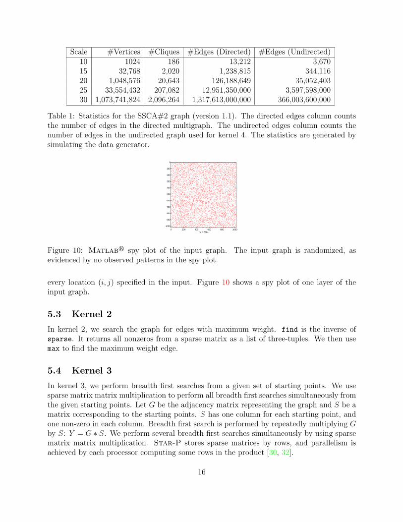
Scale #Vertices #Cliques #Edges (Directed) #Edges (Undirected)10 1024 186 13,212 3,67015 32,768 2,020 1,238,815 344,11620 1,048,576 20,643 126,188,649 35,052,40325 33,554,432 207,082 12,951,350,000 3,597,598,00030 1,073,741,824 2,096,264 1,317,613,000,000 366,003,600,000

Table 1: Statistics for the SSCA#2 graph (version 1.1). The directed edges column countsthe number of edges in the directed multigraph. The undirected edges column counts thenumber of edges in the undirected graph used for kernel 4. The statistics are generated bysimulating the data generator.

0 200 400 600 800 1000

0

100

200

300

400

500

600

700

800

900

1000

nz = 7464

Figure 10: Matlab R© spy plot of the input graph. The input graph is randomized, asevidenced by no observed patterns in the spy plot.

every location (i, j) specified in the input. Figure 10 shows a spy plot of one layer of theinput graph.

5.3 Kernel 2

In kernel 2, we search the graph for edges with maximum weight. find is the inverse ofsparse. It returns all nonzeros from a sparse matrix as a list of three-tuples. We then usemax to find the maximum weight edge.

5.4 Kernel 3

In kernel 3, we perform breadth first searches from a given set of starting points. We usesparse matrix matrix multiplication to perform all breadth first searches simultaneously fromthe given starting points. Let G be the adjacency matrix representing the graph and S be amatrix corresponding to the starting points. S has one column for each starting point, andone non-zero in each column. Breadth first search is performed by repeatedly multiplying Gby S: Y = G ∗ S. We perform several breadth first searches simultaneously by using sparsematrix matrix multiplication. Star-P stores sparse matrices by rows, and parallelism isachieved by each processor computing some rows in the product [30, 32].

16

0 200 400 600 800 1000

0

100

200

300

400

500

600

700

800

900

1000

nz = 84880 50 100 150 200 250 300

0

50

100

150

200

250

300

nz = 1934

Figure 11: The image on the left is a spy plot of the graph, reordered after clustering. Theimage on the right magnifies a portion around the diagonal. Cliques are revealed as denseblocks on the diagonal.

5.5 Kernel 4

Kernel 4 is the most interesting part of the benchmark. It can be considered to be a parti-tioning problem or a clustering problem. We have several implementations of kernel 4 basedon spectral partitioning (figure 9), “seed growing” (figure 11), and “peer pressure” algo-rithms. The peer pressure and seed growing implementations scale better than the spectralmethods, as expected. We now demonstrate how we use the infrastructure described aboveto implement kernel 4 in a few lines of Matlab R© or Star-P. Figure 11 shows a spy plotof the undirected graph after clustering. The clusters show up as dense blocks along thediagonal.

Our seed growing algorithm (figure 12) starts by picking a small set of seeds (about 2% ofthe total number of nodes) randomly. The seeds are then grown so that each seed claims allnodes reachable by at least k paths of length 1 or 2, where k is the size of the largest clique.This may cause some ambiguity, since some nodes might be claimed by multiple seeds. Wetried picking an independent set of nodes from the graph by performing one round of Luby’salgorithm [25] to keep the number of such ambiguities as low as possible. However, thequality of clustering remains unchanged when we use random sampling. We use a simpleapproach for disambiguation: the lowest numbered cluster claiming a vertex claims it. Wealso experimented with attaching singleton nodes to nearby clusters to improve the qualityof clustering.

Our peer pressure algorithm (figure 13) starts with a subset of nodes designated as leaders.There has to be at least one leader neighboring every vertex in the graph. This is followedby a round of voting where every vertex in the graph selects a leader, selecting a cluster tojoin. This does not yet yield good clustering. Each vertex now looks at its neighbors andswitches its vote to the most popular leader in its neighborhood. This last step is crucial,and in this case, it recovers more than 95% of the original clique structure of the graph.Figure 14 shows the different stages of the peer pressure algorithm on an example graph.

We experimented with different approaches to select leaders. At first, it seemed that amaximal independent set of nodes from the graph was a natural way to pick leaders. In

17

01 function J = seedgrow (seeds)

02 % Clustering by breadth first searches

03

04 % J is a sparse matrix with one seed per column.

05 J = sparse (seeds, 1:nseeds, 1, n, nseeds);

06

07 % Vertices reachable with 1 hop.

08 J = G * J;

09 % Vertices reachable with 1 or 2 hops.

10 J = J + G*J;

11 % Vertices reachable with at least k paths of 1 or 2 hops.

12 J = J >= k;

Figure 12: Breadth first parallel clustering by seed growing.

01 function cluster = peerpressure (G)

02 % Clustering by peer pressure

03

04 % Use maximal independent set routine from GAPDT

05 IS = mis (G);

06

07 % Find all neighbors in the independent set.

08 neighbors = G * sparse(IS, IS, 1, length(G), length(G));

09

10 % Each vertex chooses a random neighbor in the independent set.

11 R = sprand (neighbors);

12 [ignore, vote] = max (R, [], 2);

13

14 % Collect neighbor votes and join the most popular cluster.

15 [I, J] = find (G);

16 S = sparse (I, vote(J), 1, n, n);

17 [ignore, cluster] = max (S, [], 2);

Figure 13: Parallel clustering by peer pressure

18

Figure 14: The first graph is the input to the peer pressure algorithm. Every node thenpicks its largest numbered neighbor as a leader, as shown in the second graph. Finally, allnodes change their votes to the most popular vote amongst their neighbors, as shown in thethird graph.

practice, it turns out that simple heuristics (such as the highest numbered neighbor) gaveequally good clustering. We also experimented with more than one round of voting. Themarginal improvement in the quality of clustering was not worth the additional computationtime.

5.6 Visualization of large graphs

Graphics and visualization are a key part of an interactive system such as Matlab R©. Thequestion of how to effectively visualize large datasets in general, especially large graphs, isstill unsolved. We successfully applied methods from numerical computing to come up withmeaningful visualizations of the SSCA #2 graph.

One way to compute geometric co-ordinates for the nodes of a connected graph is to useFiedler co-ordinates [19] for the graph. Figure 9 shows the Fiedler embedding of the SSCA#2 graph. In the 2D case, we use the eigenvectors (Fiedler vectors) corresponding to thefirst two non-zero eigenvalues of the Laplacian matrix of the graph as co-ordinates for nodesof the graph in a plane.

For 3D visualization of the SSCA #2 graph, we start with 3D Fiedler co-ordinates pro-jected onto the surface of a sphere. We model nodes of the graph as particles on the surfaceof a sphere. There is a repulsive force between all particles, inversely proportional to thedistance between them. Since these particles repel each other on the surface of a sphere, weexpect them to spread around and occupy the entire surface of the sphere. Since there arecliques in the original graph, we expect clusters of particles to form on the surface of thesphere. At each timestep, we compute a force vector between all pairs of particles. Eachparticle is then displaced some distance based on its force vector. All displaced particles areprojected back onto the sphere at the end of each timestep.

This algorithm was used to generate figure 15. In this case, we simulated 256 particles

19

Matrix nr = 1024, nc = 1024, nnz = 7144Bucket nnz: max = 120, min = 0, avg = 1.74414, total = 7144, max/avg = 69

10 20 30 40 50 60

10

20

30

40

50

60

0

30

60

90

120

Figure 15: The 3D visualization of the SSCA #2 graph on the left is produced by relaxingthe Fiedler co-ordinates projected onto the surface of a sphere. The right figure shows adensity spy plot of the SSCA #2 graph.

and the system was evolved for 20 timesteps. It is important to first calculate the Fiedlerco-ordinates. Beginning with random co-ordinates results in a meaningless picture. We usedPyMOL [12] to render the graph.

5.7 Experimental Results

We ran our implementation of SSCA #2 (ver 1.1, integer only) in Star-P. The Matlab R©

client was run on a generic PC. The Star-P server was run on an SGI Altix with 128Itanium II processors with 128G RAM (total, non-uniform memory access). We used agraph generated with scale 21. This graph has 2 million nodes. The multigraph has 321million directed edges; the undirected graph corresponding to the multigraph has 89 millionedges. There are 32 thousand cliques in the graph, the largest having 128 nodes. Thereare 89 million undirected edges within cliques, and 212 thousand undirected edges betweencliques in the input graph for kernel 4. The results are presented in Fig. 16.

Our data generator scales well; the benchmark specification does not require the datagenerator to be timed. A lot of time is spent in kernel 1, where data structures for thesubsequent kernels are created. The majority of this time is spent in searching the inputtriples for duplicates, since the input graph is a multigraph. Kernel 1 creates several sparsematrices using sparse, each corresponding to a layer in the multigraph. Time spent in kernel1 also scales very well with the number of processors. Time spent in Kernel 2 also scales asexpected.

Kernel 3 does not show speedups at all. Although all the breadth first searches areperformed in parallel, the process of subgraph extraction for each starting point creates a lotof traffic between the Star-P client and the Star-P server, which are physically in differentstates. This client server communication time ends up dominating over the computationtime. This overhead can be minimized by vectorizing kernel 3 more aggressively.

Kernel 4, the non-trivial part of the benchmark, actually scales very well. We show results

20

Figure 16: SSCA #2 version 1.1 execution times (Star-P, Scale=21)

for our best performing implementation of kernel 4, which uses the seed growing algorithm.The evaluation criteria for the SSCAs also include software engineering metrics such

as code size, readability, maintainability, etc. Our implementation is extremely concise.We show the source lines of code (SLOC) for our implementation in Table 2. We alsoshow absolute line counts, which include blank lines and comments, as we believe theseto be crucial for code readability and maintainability. Our implementation runs withoutmodification in sequential Matlab R©, making it easy to develop and debug on the desktopbefore deploying on a parallel platform.

We have run the full SSCA #2 benchmark (version 0.9, integer only) on graphs with227 = 134 million nodes on the SGI Altix. Scaling results for the full benchmark (version 1.1,integer only) are presented in figure 16. We have also generated and manipulated extremelylarge graphs (1 billion nodes and 8 billion edges) on an SGI Altix with 256 processors usingStar-P.

This demonstrates that the sparse matrix representation is a scalable and efficient way tomanipulate large graphs. Not that the codes in figure 12 and figure 13 are not pseudocodes,but actual code excerpts from our implementation. Although the code fragments look verysimple and structured, the computation manipulates sparse matrices, resulting in highlyirregular communication patterns on irregular data structures.

21

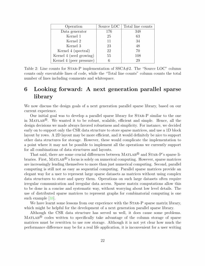
Operation Source LOC Total line countsData generator 176 348

Kernel 1 25 63Kernel 2 11 34Kernel 3 23 48

Kernel 4 (spectral) 22 70Kernel 4 (seed growing) 55 108Kernel 4 (peer pressure) 6 29

Table 2: Line counts for Star-P implementation of SSCA#2. The “Source LOC” columncounts only executable lines of code, while the “Total line counts” column counts the totalnumber of lines including comments and whitespace.

6 Looking forward: A next generation parallel sparse

library

We now discuss the design goals of a next generation parallel sparse library, based on ourcurrent experience.

Our initial goal was to develop a parallel sparse library for Star-P similar to the onein Matlab R©. We wanted it to be robust, scalable, efficient and simple. Hence, all thedesign decisions we made always favored robustness and simplicity. For instance, we decidedearly on to support only the CSR data structure to store sparse matrices, and use a 1D blocklayout by rows. A 2D layout may be more efficient, and it would definitely be nice to supportother data structures for storage. However, these would complicate the implementation toa point where it may not be possible to implement all the operations we currently supportfor all combinations of data structures and layouts.

That said, there are some crucial differences between Matlab R© and Star-P’s sparse li-braries. First, Matlab R©’s focus is solely on numerical computing. However, sparse matricesare increasingly lending themselves to more than just numerical computing. Second, parallelcomputing is still not as easy as sequential computing. Parallel sparse matrices provide anelegant way for a user to represent large sparse datasets as matrices without using complexdata structures to store and query them. Operations on such large datasets often requireirregular communication and irregular data access. Sparse matrix computations allow thisto be done in a concise and systematic way, without worrying about low level details. Theuse of distributed sparse matrices to represent graphs for combinatorial computing is onesuch example [33].

We have learnt some lessons from our experience with the Star-P sparse matrix library,which might be helpful for the development of a next generation parallel sparse library.

Although the CSR data structure has served us well, it does cause some problems.Matlab R© codes written to specifically take advantage of the column storage of sparsematrices must be rewritten to use row storage. Although it is not yet clear how much theperformance difference may be for a real life application, it is inconvenient for a user writing

22

highly tuned codes using sparse matrices. Such a code will also have different performancecharacteristics in Matlab R© and Star-P.

We propose adding a third design principle to the two stated in section 4. The differencein performance between accessing a sparse matrix by rows or columns must be minimal.Users writing sparse matrix codes should not have to worry about organizing their sparsematrix accesses by rows or columns, just as they do not worry about how dense matrices arestored.

For an example of the third principle, consider the operation below. It is much simplerto extract the submatrix specified by p from a matrix stored in the CSR format than froma matrix stored in the CSC format. In the latter case, a binary search is required for everycolumn, making the operation slower.

>> A = S(p, :) % p is a vector

A parallel sparse library that needs to scale to hundreds or thousands of processorswill not work well with a one-dimensional block layout. A two-dimensional block layoutis essential for scalability of several sparse matrix operations. The benefits of 2D layoutsare well known at this point, and we will not reiterate them. It is important to note thatcompressed row/column data structures are not efficient for storing sparse matrices in a 2Dlayout.

Another point of departure is a different primitive for indexing operations. Currently,we use the “sparse-find” method to perform all the indexing operations such as submatrixindexing, assignment, concatenation and transpose. We used the concept of the sparse

function as a primitive using which we built the rest of the operations. We propose that anext generation sparse matrix library should use sparse matrix multiplication as the basicprimitive in the library.

We illustrate the case of submatrix indexing using matrix multiplication. Suppose A isa matrix, and we wish to extract the submatrix B = A(I, J). Multiplying from the leftpicks out the rows, while multiplying from the right picks out the columns, as shown in codefragment 17.

We believe that it will be possible to implement sparse matrix multiplication more ef-ficiently with a 2D block distribution than a 1D block distribution for large numbers ofprocessors. Indexing operations may then be implemented using sparse matrix multiplica-tion as a primitive. An efficient sparse matrix multiplication implementation might actuallyuse a polyalgorithm to simplify the implementation for special cases when more informa-tion is available about the structure of matrices being multiplied, as is the case for indexingoperations.

The choice of a suitable data structure to store sparse matrices in a 2D block layout andallow efficient matrix multiplication still remains an open question for future research. Webelieve that once the right data structure is selected, there will not be a large differencein performance when multiplying from the left or the right. This directly translates intosymmetric performance for all indexing operations when accessing a matrix either by rowsor columns. We believe this will lead to higher programmer productivity, freeing users from

23

01 function B = index by mult (A, I, J)

02 % Index a matrix with matrix multiplication

03

04 [nrows, nccols] = size(A);

05 nI = length(I);

06 nJ = length(J);

07

08 % Multiply on the left to pick the required rows

09 row select = sparse(1:nI, I, 1, nI, nr);

10

11 % Multiply on the right to pick the required columns

12 col select = sparse(J, 1:nJ, 1, nc, nJ);

13

14 % Compute B with sparse matrix multiplication

15 B = row select * A * col select;

Figure 17: Matrix indexing and concatenation can be implemented using sparse matrix-matrix multiplication as a primitive. Multiplication from the left picks the necessary rows,while multiplication from the right picks the necessary columns.

tuning their codes in specific ways that depend on knowledge of the underlying implemen-tation of indexing operations.

7 Conclusion

We described the design and implementation of a distributed sparse matrix infrastructure inStar-P. This infrastructure was used to build the “Graph Algorithms and Pattern DiscoveryToolbox (GAPDT)”. We demonstrated the effectiveness of our tools by implementing a graphanalysis benchmark in Star-P, which scales to large problem sizes on large processor counts.

We conclude that distributed sparse matrices provide a powerful set of primitives fornumerical and combinatorial computing. We hope that the our experiences will shape thedesign of future parallel sparse matrix infrastructures in other languages.

24

References

[1] P. Amestoy, I. S. Duff, and J.-Y. L’Excellent. Multifrontal solvers within the PARASOLenvironment. In PARA, pages 7–11, 1998.

[2] E. Anderson, Z. Bai, C. Bischof, S. Blackford, J. Demmel, J. Dongarra, J. Du Croz,A. Greenbaum, S. Hammarling, A. McKenney, and D. Sorensen. LAPACK Users’ Guide.Society for Industrial and Applied Mathematics, Philadelphia, PA, third edition, 1999.

[3] D. Bader, J. Feo, J. Gilbert, J. Kepner, D. Koester, E. Loh, K. Madduri, B. Mann, andT. Meuse. HPCS scalable synthetic compact applications #2. version 1.1.

[4] D. A. Bader, K. Madduri, J. R. Gilbert, V. Shah, J. Kepner, T. Meuse, and A. Kr-ishnamurthy. Designing scalable synthetic compact applications for benchmarking highproductivity computing systems. Cyberinfrastructure Technology Watch, Nov 2006.

[5] D. H. Bailey, E. Barszcz, J. T. Barton, D. S. Browning, R. L. Carter, D. Dagum, R. A.Fatoohi, P. O. Frederickson, T. A. Lasinski, R. S. Schreiber, H. D. Simon, V. Venkatakr-ishnan, and S. K. Weeratunga. The NAS parallel benchmarks. The International Journalof Supercomputer Applications, 5(3):63–73, Fall 1991.

[6] T. F. Chan, J. R. Gilbert, and S.-H. Teng. Geometric spectral partitioning. TechnicalReport CSL-94-15, Palo Alto Research Center, Xerox Corporation, 1994.

[7] Y. Chen, T. A. Davis, W. W. Hager, and S. Rajamanickam. Algorithm 8xx: Cholmod,supernodal sparse cholesky factorization and update/downdate. Technical Report TR-2006-005, University of Florida, 2006. Submitted to ACM Transactions on MathematicalSoftware.

[8] R. Choy and A. Edelman. Parallel MATLAB: doing it right. Proceedings of the IEEE,93:331–341, Feb 2005.

[9] E. Cohen. Structure prediction and computation of sparse matrix products. Journal ofCombinatorial Optimization, 2(4):307–332, 1998.

[10] T. A. Davis. Algorithm 832: Umfpack v4.3—an unsymmetric-pattern multifrontalmethod. ACM Transactions on Mathematical Software, 30(2):196–199, 2004.

[11] T. A. Davis. Direct Methods for Sparse Linear Systems (Fundamentals of Algorithms2). Society for Industrial and Applied Mathematics, Philadelphia, PA, USA, 2006.

[12] W. L. DeLano and S. Bromberg. The PyMOL User’s Manual. DeLano Scientific LLC,San Carlos, CA, USA., 2004.

[13] J. J. Dongarra. Performance of various computers using standard linear equations soft-ware in a FORTRAN environment. SIGARCH Computer Architecture News, 16(1):47–69, 1988.

25

[14] R. D. Falgout, J. E. Jones, and U. M. Yang. The design and implementation of hypre, alibrary of parallel high performance preconditioners. Design document from the hyprehomepage.

[15] J. R. Gilbert, C. Moler, and R. Schreiber. Sparse matrices in MATLAB: Design andimplementation. SIAM Journal on Matrix Analysis and Applications, 13(1):333–356,1992.

[16] J. R. Gilbert, S. Reinhardt, and V. Shah. An interactive environment to manipulatelarge graphs. In Proceedings of the 2007 IEEE International Conference on Acoustics,Speech, and Signal Processing, April 2007.

[17] J. R. Gilbert and S.-H. Teng. Matlab mesh partitioning and graph separator toolbox,2002. http://www.cerfacs.fr/algor/Softs/MESHPART/index.html.

[18] F. G. Gustavson. Two fast algorithms for sparse matrices: Multiplication and permutedtransposition. ACM Transactions on Mathematical Software, 4(3):250–269, 1978.

[19] K. Hall. An r-dimensional quadratic placement algorithm. Management Science,17(3):219–229, Nov 1970.

[20] P. Husbands. Interactive supercomputing. PhD thesis, Massachussetts Institute of Tech-nology, 1999.

[21] P. Husbands, C. Isbell, and A. Edelman. MITMatlab: A tool for interactive supercom-puting. In SIAM Conference on Parallel Processing for Scientific Computing, 1999.

[22] R. Ihaka and R. Gentleman. R: A language for data analysis and graphics. Journal ofComputational and Graphical Statistics, 5(3):299–314, 1996.

[23] Interactive Supercomputing LLC. Star-P Software Development Kit (SDK): Tutorialand Reference Guide, 2007. version 2.5.

[24] X. S. Li and J. W. Demmel. SuperLU DIST: A scalable distributed memory sparse directsolver for unsymmetric linear systems. ACM Transactions on Mathematical Software,29(2):110–140, 2003.

[25] M. Luby. A simple parallel algorithm for the maximal independent set problem. InSTOC ’85: Proceedings of the seventeenth annual ACM symposium on Theory of com-puting, pages 1–10, New York, NY, USA, 1985. ACM Press.

[26] K. Maschhoff and D. Sorensen. A portable implementation of ARPACK for distributedmemory parallel archituectures. Proceedings of Copper Mountain Conference on Itera-tive Methods, Apr 1996.

[27] Mathworks Inc. MATLAB User’s Guide, 2007. version 2007a.

26

[28] A. Pothen, H. D. Simon, and K.-P. Liou. Partitioning sparse matrices with eigenvectorsof graphs. SIAM Journal of Matrix Analysis and Applications, 11(3):430–452, 1990.

[29] S. Reinhardt, J. R. Gilbert, and V. Shah. High performance graph algorithms fromparallel sparse matrices. In Proceedings of the Workshop on state of the art in scientificand parallel computing, 2006.

[30] C. Robertson. Sparse parallel matrix multiplication. Master’s thesis, UC Santa Barbara,2005.

[31] J. N. Shadid and R. S. Tuminaro. Sparse iterative algorithm software for large-scaleMIMD machines: An initial discussion and implementation. Concurrency: Practice andExperience, 4(6):481–497, 1992.

[32] V. Shah and J. R. Gilbert. Sparse matrices in Matlab*P: Design and implementation. InL. Bouge and V. K. Prasanna, editors, HiPC, volume 3296 of Lecture Notes in ComputerScience, pages 144–155. Springer, 2004.

[33] V. B. Shah. An Interactive System for Combinatorial Scientific Computing with anEmphasis on Programmer Productivity. PhD thesis, University of California, SantaBarbara, June 2007.

[34] G. van Rossum. Python Reference Manual. Python Software Foundation, 2006. version2.5.

27