i

UNIVERSITY OF CALIFORNIA, SAN DIEGO

Distributed Proxy-Layer Scheduling in Heterogeneous Wireless Sensor Networks

A thesis submitted in partial satisfaction of the requirements for the degree Master of Science

in

Computer Science

by

Daeseob Lim

Committee in charge: Professor Tajana Simunic Rosing, Chair Professor Geoffrey Michael Voelker Professor Tara Javidi

2007

ii

Copyright

Daeseob Lim, 2007

All rights reserved.

iii

The Thesis of Daeseob Lim is approved:

Chair

University of California, San Diego

2007

iii

iv

TABLE OF CONTENTS

SIGNATURE PAGE......................................................................................................iii

TABLE OF CONTENTS............................................................................................... iv

LIST OF FIGURES.......................................................................................................vi

ACKNOWLEDGEMENTS ........................................................................................viii

ABSTRACT OF THE THESIS ..................................................................................... ix

I. INTRODUCTION ...................................................................................................1

II. RELATED WORK...................................................................................................7

III. MOTIVATION.......................................................................................................12

1. IEEE 802.11 MAC.................................................................................................... 12

2. Performance degradation due to contention.............................................................. 15

3. Interference in a multi-cell wireless network............................................................ 18

IV. SCHEDULING ALGORITHM .............................................................................22

1. Optimal node-level scheduling ................................................................................. 24

2. Centralized node-level scheduling (CNLS) .............................................................. 34

3. Distributed node-level scheduling (DNLS) .............................................................. 38

4. Cell-level scheduling ................................................................................................ 42

5. Combined running of cell-level and node-level scheduling ..................................... 44

V. SIMULATION AND EVALUATION....................................................................48

1. Proxy layer design .................................................................................................... 48

2. Simulation setup ....................................................................................................... 49

3. Results for the CBR traffic in full MAC queues....................................................... 52

iv

v

4. Results for the real data traffic.................................................................................. 56

VI. CONCLUSIONS ...................................................................................................63

VII. REFERENCES ......................................................................................................65

v

vi

LIST OF FIGURES

Figure 1. Network topology of HPWREN.......................................................................... 2

Figure 2. SMER network .................................................................................................... 3

Figure 3. Structure of the heterogeneous wireless network composed of three layers ....... 4

Figure 4. 802.11 DCF model............................................................................................. 13

Figure 5. Aggregate throughput with different number of wireless nodes........................ 16

Figure 6. Congestion on MAC layer ................................................................................. 17

Figure 7. Measurement of throughput and interference in a multi-cell wireless network 20

Figure 8. The architecture of a heterogeneous wireless network ...................................... 22

Figure 9. Contention graph constructed from Figure 8..................................................... 23

Figure 10. Conversion from G to G’ and the maximum clique of size 4. ......................... 27

Figure 11. Conversion from G to G′ , for s = 2................................................................. 30

Figure 12. Maximal time slot assignment, s = 1 ............................................................. 35

Figure 13. Maximal scheduling, s = 2............................................................................. 37

Figure 14. Example of running DNLS at 10v ................................................................... 40

Figure 15. A cell in network topology and two examples of multi-cell networks ............ 43

Figure 16. Examples of cell-level scheduling ................................................................... 45

Figure 17. Combined running of cell-level and node-level scheduling ............................ 46

Figure 18. Implementation of scheduler and proxy .......................................................... 49

Figure 19. Multi-cell topology used in simulations .......................................................... 51

Figure 20.Results for the CBR traffic model .................................................................... 53

Figure 21. Two strategies for cell-level scheduling in square multi-cell .......................... 55

Figure 22. Results for the real traffic data model.............................................................. 58

vi

vii

Figure 23. Application layer delay in a real-traffic model ................................................ 59

Figure 24. Throughput and power for different slot sizes ................................................. 61

vii

viii

ACKNOWLEDGEMENTS

I would first like to thank my research advisor, Tajana Simunic Rosing. Her

guidance has been invaluable through all stages of this thesis. The advice from Tara

Javidi and Geoffrey Michael Voelker has been greatly helpful in designing the

algorithms proposed in this thesis.

I would like to thank the HPWREN project and the NSF for their support.

HPWREN is based on the work sponsored by the National Science Foundation and its

ANIR division under Grant Number 0426879. I also thank Hans-Werner Braun from

the San Diego Supercomputer Center (SDSC) and Pablo Bryant from the San Diego

State University for their help and support for the research on the HPWREN/SMER

project.

I want to express my sincere gratitude to my family. I thank my mother for the

sacrifices she made. My sisters always showed their faith and encouragement to me.

Without their devotion, I may never have completed this thesis or even my graduate

degree. Thank you for your love and support. And I thank God.

viii

ix

ABSTRACT OF THE THESIS

Distributed Proxy-Layer Scheduling in Heterogeneous Wireless Sensor Networks

by

Daeseob Lim

Master of Science in Computer Science

University of California, San Diego, 2007

Professor Tajana Simunic Rosing, Chair

In this thesis, we present a distributed hybrid multi-cell scheduling algorithm for

heterogeneous wireless sensor networks. The proposed scheduling algorithm addresses

the issues of limited power on mobile nodes and throughput degradation due to

contention in multi-cell wireless networks. Our scheduling algorithm consists of two

parts; cell-level scheduling and node-level scheduling.

The cell-level scheduling algorithm decides which cells are active so that the

interference between active cells is reduced drastically. Node-level scheduling

ix

x

algorithm decreases the contention among wireless nodes by limiting the number of

active nodes accessing a wireless channel. By combining these two scheduling

algorithms, we reduce energy consumption of communication devices on mobile

nodes and improve aggregate throughput in multi-cell wireless networks.

The proposed scheduling algorithm is designed to run in a distributed manner.

To show the efficiency of our node-level algorithm, we first give, for comparison, an

optimal node-level scheduling algorithm and show that the problem is NP-complete.

Finally, we present a heuristic scheduling algorithm and convert it into our distributed

node-level scheduling algorithm.

We also evaluate the performance of our algorithm. Simulation results from the

ns-2 network simulator show that our scheduling is effective in saving communication

power while improving throughput of multi-cell wireless networks. Our scheduling

achieves a throughput improvement of up to 10.31% and maximum power saving of

85.54%.

x

1

I. INTRODUCTION

A heterogeneous wireless network is a wireless network system consisting of devices

with various levels of computing capability, different energy constraints, and multiple types of

wireless connectivity. When heterogeneous wireless networks are constructed over sensor

networks, we call them heterogeneous wireless sensor networks. Similar to typical wireless

networks, heterogeneous wireless sensor networks suffer from limited battery lifetime,

excessive contention between wireless nodes, and insufficient network throughput capacity.

Often heterogeneous wireless sensor network applications also have variety of quality of

service (QoS) requirements.

To have wide coverage in the field and to successfully transfer heavy traffic from the

sensor nodes, heterogeneous wireless sensor networks use high-bandwidth connections

centered at sensor node cluster heads over the underlying sensor network. Once the traffic

from the sensor nodes is collected at cluster heads, the wireless network delivers the data to a

wired network backbone. Commercial wireless LAN (WLAN) such as IEEE 802.11 is a good

candidate for the relay network which connects the cluster header nodes with a wired network.

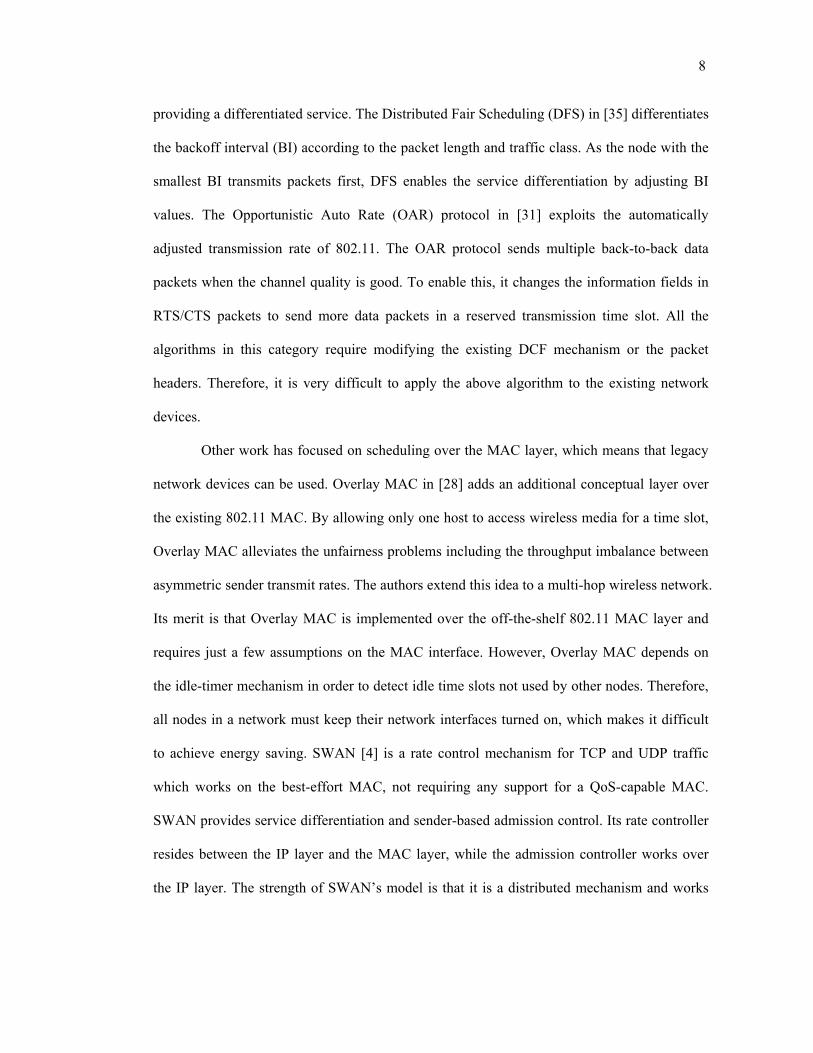
An example of a heterogeneous wireless sensor network is the High-Performance

Wireless Research and Education Network (HPWREN) [2] deployed in the Southern

California area. As shown in Figure 1, HPWREN connects local universities, research

institutes, and natural observatories through a variety of wireless and backbone networks. In

HPWREN, there are many kinds of computing systems ranging from the small wireless sensor

nodes, and scientists’ laptops, to the high-performance server systems at the San Diego

Supercomputer Center. HPWREN has several subnetworks in it. One of them is the Santa

Margarita Ecological Reserve (SMER) network in Figure 2, which is a good example of a

1

2

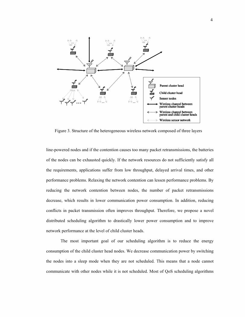
heterogeneous wireless sensor network.

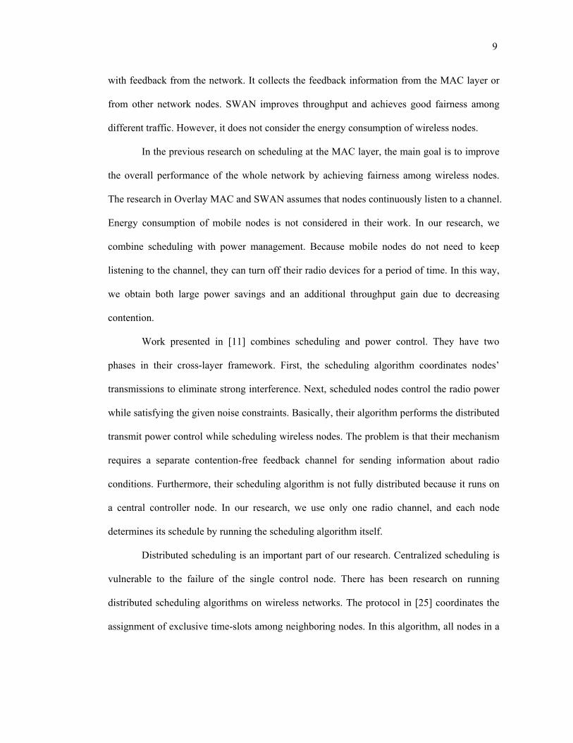
The SMER network consists of three layers of deployed wireless nodes. The lowest

layer collects ecological information in the field and transfers the data to the middle layer

through a typical sensor network. The middle layer is a group of child cluster heads (child

CHs) which convey the data from sensor nodes to the parent cluster heads (parent CHs)

through a faster wireless connection, mainly IEEE 802.11b. This middle layer is responsible

for handling the heavy traffic of the underlying sensors. In this layer, the issues such as

contention and interference between adjacent wireless nodes result in insufficient throughput

capacity. The parent cluster heads in the upper layer connects child cluster heads to the

HPWREN wireless mesh backbone.

One of the important issues in heterogeneous wireless sensor networks is the battery

life of mobile wireless nodes. Typically, a large portion of the total energy in mobile devices

is consumed by the wireless communication devices. In particular, the radio power

Figure 1. Network topology of HPWREN

3

consumption in an idle state of wireless devices plays a significant role in the lifetime of

mobile devices. In the case of heavy congestion in a wireless channel, the issue of

communication power is even more important. For example, in the middle layer of the SMER

network, a parent cluster head incorporates many child cluster heads. As the child cluster

heads are close to each other, their radio signals cause a high rate of interference, which

results in a large number of packet collisions. Moreover, adjacent child cluster heads that join

different parent cluster heads can also interfere over the same radio channel. Channel

assignment may reduce the interference in the shared channels (e.g. channel interference in

cellular networks). As the number of usable non-interfered channels is limited, the channel

assignment cannot solve the interference problem completely.

In the SMER network, for example, a dense distribution of network devices and the

diversity of their characteristics cause performance problems. The contention increases as

more network devices are deployed into the field. The diversity in energy consumption and

power supply makes the problem more complex. If the nodes with battery power contend with

Figure 2. SMER network

4

line-powered nodes and if the contention causes too many packet retransmissions, the batteries

of the nodes can be exhausted quickly. If the network resources do not sufficiently satisfy all

the requirements, applications suffer from low throughput, delayed arrival times, and other

performance problems. Relaxing the network contention can lessen performance problems. By

reducing the network contention between nodes, the number of packet retransmissions

decrease, which results in lower communication power consumption. In addition, reducing

conflicts in packet transmission often improves throughput. Therefore, we propose a novel

distributed scheduling algorithm to drastically lower power consumption and to improve

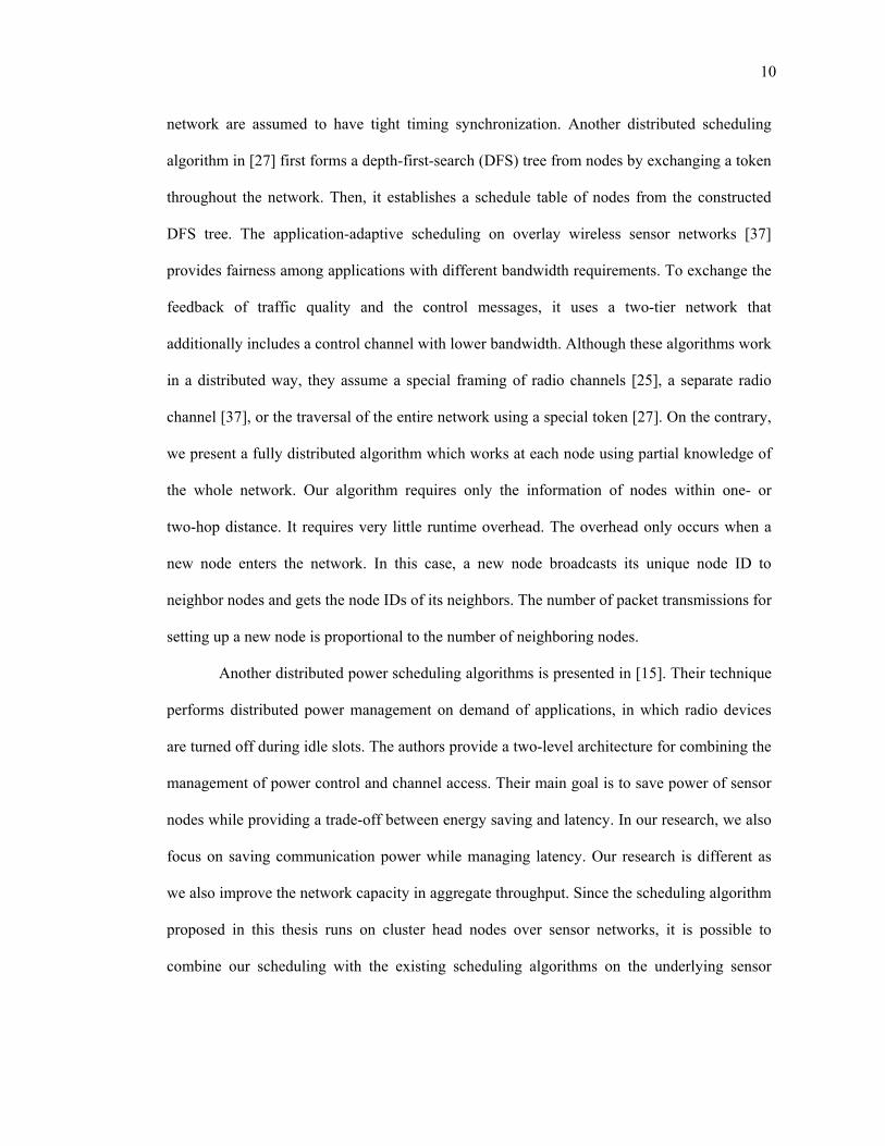
network performance at the level of child cluster heads.

The most important goal of our scheduling algorithm is to reduce the energy

consumption of the child cluster head nodes. We decrease communication power by switching

the nodes into a sleep mode when they are not scheduled. This means that a node cannot

communicate with other nodes while it is not scheduled. Most of QoS scheduling algorithms

… …

…

Sensor nodes

Child cluster head

Parent cluster head

Wireless channel between parent cluster heads

Wireless channel between parent and child cluster heads

Wireless sensor network

…

……

… ……

……

Sensor nodes

Child cluster head

Parent cluster head

Wireless channel between parent cluster heads

Wireless channel between parent and child cluster heads

Wireless sensor network

Sensor nodes

Child cluster head

Parent cluster head

Wireless channel between parent cluster heads

Wireless channel between parent and child cluster heads

Wireless sensor network

……

…………

Figure 3. Structure of the heterogeneous wireless network composed of three layers

5

for wireless networks use feedback or notifications from adjacent nodes at runtime. In that

case, they require that the network interface is always active (turned on). For example,

Overlay MAC in [28] successfully implements the distributed scheduling of 802.11 wireless

nodes. The Overlay MAC, however, depends on a timer expiration mechanism to detect the

idleness of a wireless channel. If we intend to save energy in communication devices, it is not

easy to rely on timer expirations in the MAC layer. In heterogeneous wireless sensor networks,

battery-powered wireless nodes need to put their wireless interfaces to sleep for a long time

because power saving is a main concern in this type of wireless network. For this reason, the

distributed scheduling algorithms we have developed are designed to work even if a network

interface is not always active.

The goal of the scheduling algorithm presented in this thesis is to increase the battery

lifetime of wireless nodes while maximizing the efficiency of bandwidth utilization in a

hierarchical heterogeneous wireless sensor network. For this goal, we run a hybrid distributed

scheduling algorithm that consists of two scheduling parts. At a cell level, we choose active

cells that do not interfere with other scheduled cells. We allow only the nodes in scheduled

active cells to access a wireless channel. At a node level, we control the number of nodes

simultaneously accessing wireless media. The node-level scheduler decides which nodes in

active cells are allowed to access the media.

To simplify the problem and to effectively target the layers with the most significant

performance issues, we focus on the middle layer of the heterogeneous wireless networks;

child cluster heads and parent cluster heads. We assume that appropriate scheduling and

routing algorithms handle data delivery from sensors to a child cluster head in the lower layer.

Child cluster heads deliver the collected sensing data to their parent cluster heads. Parent

cluster heads form a mesh network by connecting to each other.

6

Our proposed scheduling algorithm runs in a proxy layer. The scheduler resides

between OS kernel and user applications. The proxy is transparent to the applications running

on the wireless nodes. For applications, the proxy layer is very similar to kernel protocol

layers. Since legacy applications do not have to recognize its existence, they can work over the

proxy layer with minimum modification. In addition, proxy layer implementation over

transport/network layers does not require modifying MAC or kernel protocol implementation.

Thus, the scheduling in the proxy layer is not dependent on the physical mechanism of

wireless network systems. Therefore, our approach is very flexible and applicable to different

types of wireless networks. In simulation results, we see a throughput improvement of up to

10.31% and maximum power saving of 85.54%.

The remainder of the thesis is organized as follows: we summarize the related work in

the next chapter. Motivations for this research are introduced in Chapter III. Our new

scheduling algorithms are presented in Chapter IV. In Chapter V, the simulation setup and the

simulation results for our scheduling algorithm are presented. Finally, we conclude our

discussion in Chapter VI.

7

II. RELATED WORK

There has been a significant amount of research on performance and quality of service

(QoS) of wireless networks. The research on throughput degradation explains why and how

packet collisions affect throughput in wireless networks. Many scheduling algorithms have

been developed to improve throughput, to reduce energy consumption in communication, and

eventually to provide a better framework for meeting requirements for QoS.

The problem of throughput degradation in a wireless network has been investigated in

detail. In [17], the maximum theoretical bandwidth is calculated from the given MAC scheme,

MSDU size, modulation scheme, and data rate. In the actual networks, however, there are

multiple wireless nodes. The interaction and interference between nodes prevent the network

from achieving its maximum bandwidth. As the number of contending nodes increases, the

aggregate throughput falls gradually because collisions between nodes happen more

frequently and the backoff time increases due to a longer contention window [14]. This

performance degradation becomes even worse in real networks [8] [36] because 802.11 MAC

lowers its transmission rate according to the channel quality. This may cause severe

performance degradation.

Many algorithms have been proposed to solve the performance degradation problem

in wireless networks. The first approach to this problem is to revise MAC layer algorithms.

The original DCF algorithm cannot give prioritized service to user. Enhanced DCF (EDCF)

[22] prioritizes traffic categories with different contention parameters. According to the

priorities, a wireless node can implement up to eight transmission queues. Each transmission

queue has different parameters for deciding its backoff time. With this, EDCF gives more

chance of channel access to high priority traffic. EDCF is compatible with legacy DCF while

7

8

providing a differentiated service. The Distributed Fair Scheduling (DFS) in [35] differentiates

the backoff interval (BI) according to the packet length and traffic class. As the node with the

smallest BI transmits packets first, DFS enables the service differentiation by adjusting BI

values. The Opportunistic Auto Rate (OAR) protocol in [31] exploits the automatically

adjusted transmission rate of 802.11. The OAR protocol sends multiple back-to-back data

packets when the channel quality is good. To enable this, it changes the information fields in

RTS/CTS packets to send more data packets in a reserved transmission time slot. All the

algorithms in this category require modifying the existing DCF mechanism or the packet

headers. Therefore, it is very difficult to apply the above algorithm to the existing network

devices.

Other work has focused on scheduling over the MAC layer, which means that legacy

network devices can be used. Overlay MAC in [28] adds an additional conceptual layer over

the existing 802.11 MAC. By allowing only one host to access wireless media for a time slot,

Overlay MAC alleviates the unfairness problems including the throughput imbalance between

asymmetric sender transmit rates. The authors extend this idea to a multi-hop wireless network.

Its merit is that Overlay MAC is implemented over the off-the-shelf 802.11 MAC layer and

requires just a few assumptions on the MAC interface. However, Overlay MAC depends on

the idle-timer mechanism in order to detect idle time slots not used by other nodes. Therefore,

all nodes in a network must keep their network interfaces turned on, which makes it difficult

to achieve energy saving. SWAN [4] is a rate control mechanism for TCP and UDP traffic

which works on the best-effort MAC, not requiring any support for a QoS-capable MAC.

SWAN provides service differentiation and sender-based admission control. Its rate controller

resides between the IP layer and the MAC layer, while the admission controller works over

the IP layer. The strength of SWAN’s model is that it is a distributed mechanism and works

9

with feedback from the network. It collects the feedback information from the MAC layer or

from other network nodes. SWAN improves throughput and achieves good fairness among

different traffic. However, it does not consider the energy consumption of wireless nodes.

In the previous research on scheduling at the MAC layer, the main goal is to improve

the overall performance of the whole network by achieving fairness among wireless nodes.

The research in Overlay MAC and SWAN assumes that nodes continuously listen to a channel.

Energy consumption of mobile nodes is not considered in their work. In our research, we

combine scheduling with power management. Because mobile nodes do not need to keep

listening to the channel, they can turn off their radio devices for a period of time. In this way,

we obtain both large power savings and an additional throughput gain due to decreasing

contention.

Work presented in [11] combines scheduling and power control. They have two

phases in their cross-layer framework. First, the scheduling algorithm coordinates nodes’

transmissions to eliminate strong interference. Next, scheduled nodes control the radio power

while satisfying the given noise constraints. Basically, their algorithm performs the distributed

transmit power control while scheduling wireless nodes. The problem is that their mechanism

requires a separate contention-free feedback channel for sending information about radio

conditions. Furthermore, their scheduling algorithm is not fully distributed because it runs on

a central controller node. In our research, we use only one radio channel, and each node

determines its schedule by running the scheduling algorithm itself.

Distributed scheduling is an important part of our research. Centralized scheduling is

vulnerable to the failure of the single control node. There has been research on running

distributed scheduling algorithms on wireless networks. The protocol in [25] coordinates the

assignment of exclusive time-slots among neighboring nodes. In this algorithm, all nodes in a

10

network are assumed to have tight timing synchronization. Another distributed scheduling

algorithm in [27] first forms a depth-first-search (DFS) tree from nodes by exchanging a token

throughout the network. Then, it establishes a schedule table of nodes from the constructed

DFS tree. The application-adaptive scheduling on overlay wireless sensor networks [37]

provides fairness among applications with different bandwidth requirements. To exchange the

feedback of traffic quality and the control messages, it uses a two-tier network that

additionally includes a control channel with lower bandwidth. Although these algorithms work

in a distributed way, they assume a special framing of radio channels [25], a separate radio

channel [37], or the traversal of the entire network using a special token [27]. On the contrary,

we present a fully distributed algorithm which works at each node using partial knowledge of

the whole network. Our algorithm requires only the information of nodes within one- or

two-hop distance. It requires very little runtime overhead. The overhead only occurs when a

new node enters the network. In this case, a new node broadcasts its unique node ID to

neighbor nodes and gets the node IDs of its neighbors. The number of packet transmissions for

setting up a new node is proportional to the number of neighboring nodes.

Another distributed power scheduling algorithms is presented in [15]. Their technique

performs distributed power management on demand of applications, in which radio devices

are turned off during idle slots. The authors provide a two-level architecture for combining the

management of power control and channel access. Their main goal is to save power of sensor

nodes while providing a trade-off between energy saving and latency. In our research, we also

focus on saving communication power while managing latency. Our research is different as

we also improve the network capacity in aggregate throughput. Since the scheduling algorithm

proposed in this thesis runs on cluster head nodes over sensor networks, it is possible to

combine our scheduling with the existing scheduling algorithms on the underlying sensor

11

networks.

Maximizing network capacity, while reducing interference between wireless nodes, is

a long-standing issue in multi-cell wireless networks. When a network consists of multiple

cells, a channel assignment scheme increases the capacity of the network throughput by

allocating different radio channels to adjacent cells. However, the limited availability of radio

channels makes channel assignment a challenge. The channel assignment problem in

multi-cell networks has been shown to be equivalent to a graph-coloring problem in [13] and

[29]. On a given channel, the problem of maximizing the limited capacity of aggregate

throughput has been studied extensively. One solution is to control the transmit power of

wireless interface devices shown in [43]. A transmit power control scheme is effective in

maximizing the number of simultaneous connections in a network channel. However, the

accurate control of transmit power requires the access to network interface devices and the

knowledge of signal power on physical/link layers. It is also common that the transmit power

control scheme needs a separate feedback channel. The runtime overhead for delivering

feedback information is not negligible. In this research, we do not use the transmit power

control of wireless interface devices. Instead, we control the channel access of cells on a high

level and the channel access of nodes on a lower level. In the proposed scheduling algorithm,

only the scheduled nodes in the active cells are allowed to access the channel.

In order to run the proposed scheduling algorithm over kernel protocol layers, we use

a proxy layer. In other words, our scheduling algorithm runs over the existing transport layer.

In general, proxies are widely used for caching web traffic or multimedia data [42] [30] .

Because of its adaptability to legacy systems, proxies are also used for frameworks supporting

high-level traffic management, such as service differentiation of streaming traffic in [32]. The

proxy provides transparency of interface to the applications. It is also easy to implement new

scheduling policies in the proxy without modifying the implementation of lower layers.

12

III. MOTIVATION

In this chapter, we motivate our research. As explained in Chapter I, our research

focuses on achieving power saving while providing higher network throughput capacity. Our

target network, the SMER network in HPWREN [2], has IEEE 802.11 wireless connections

between cluster head nodes deployed in the Santa Margarita Ecological Reserve. IEEE 802.11

is a good example of high speed wireless networks, and it is suitable for establishing

connections among cluster heads. However, wireless channels between cluster heads often

suffer from the lack of network throughput due to a large amount of data traffic collected from

sensor nodes. In a typical multi-cell wireless network, performance degradation is caused by

both contention between nodes and interference between cells. In the first section of this

chapter, we summarize the underlying mechanism of IEEE 802.11 MAC, in particular its DCF

access mode. In the next section, we examine the performance degradation problem caused by

excessive contention between the nodes in a single-cell network. In the last section, we study

the details of interference between neighboring cells.

1. IEEE 802.11 MAC

IEEE 802.11 defines two types of network service models. Independent BSS (Basic

Service Set), called IBSS or ad hoc network, is composed of independent node stations. In

IBSS, the nodes communicate directly with each other without an access point. On the

contrary, an infrastructure BSS, commonly called infrastructure mode, uses an access point. In

the infrastructure BSS, all wireless communication occurs between access points and mobile

nodes. When a mobile node sends data to another node, data is delivered through an access

point. Currently, the 802.11 infrastructure BSS is the more popular wireless network model in

the market. In this thesis, all discussions about wireless network services refer to the

12

13

infrastructure BSS.

In 802.11 MAC, there are two well-known MAC access modes; a point coordination

function (PCF) and a distributed coordination function (DCF). Even though PCF provides

contention-free services, it is not widely implemented among 802.11 devices in the market.

DCF uses the standard CSMA/CA access mechanism. It is possible to use the RTS/CTS

technique with DCF to reduce the possibility of collisions. However, the RTS/CTS

mechanism incurs overhead due to additional frame transmissions. Because of this overhead,

the actual throughput in RTS/CTS mode is lower than it is without RTS/CTS. Therefore, use

of RTS/CTS is usually limited to relatively long size packets. The threshold for RTS/CTS is

set as a RTS threshold. In practice, almost all frames are limited to a size smaller than RTS

threshold by the Ethernet MTU value or by TCP fragmentation. In most of practical wireless

networks, the RTS/CTS mechanism is not widely used because of its overhead from additional

packet transmissions. In this thesis, we do not use the RTS/CTS mechanism.

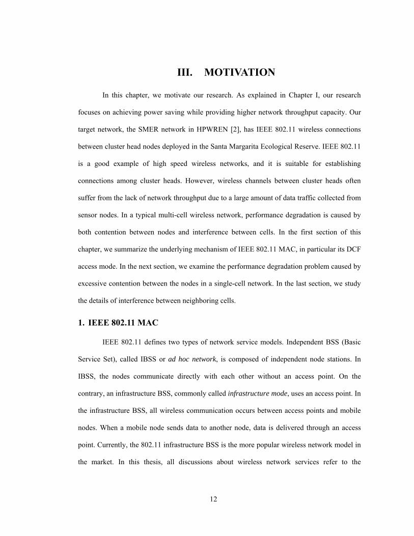
In the DCF mode, wireless nodes compete with others to access a wireless channel.

DIFSDIFS DIFS

Frame

Frame

Frame

Station A

Station B

Station C

Station D

Station E

Frame

Defer

Defer

Defer

Defer

Defer

Defer

Defer

Defer Defer

Backoff timeBackoff time remainingArrival of data

DIFSDIFSDIFSDIFSDIFSDIFS DIFSDIFSDIFS

FrameFrame

FrameFrame

FrameFrame

Station A

Station B

Station C

Station D

Station E

Station A

Station B

Station C

Station D

Station E

FrameFrame

Defer

Defer

Defer

Defer

Defer

Defer

Defer

Defer Defer

Backoff timeBackoff time remainingArrival of data

Backoff timeBackoff time remainingArrival of data

Backoff timeBackoff time remainingArrival of data

Figure 4. 802.11 DCF model

14

Before getting the right of access, a node waits for some time to check if any other nodes are

accessing the channel. If other nodes are accessing the channel, all the other nodes that want to

use the wireless media should wait for the channel to be idle. This is called access deferral.

Access deferral does not end immediately after the channel becomes idle; however, it leaves

an interframe space. The interframe space refers to an additional deferral after the

transmission of a frame. To give different priority levels to frame types, interframe spacings

vary among frame transmissions. Figure 4 shows how access deferral and interframe spacing

work. For simplicity, only data frame type is drawn. In the actual 802.11 MAC, an ACK

frame follows a data frame transmission. Interframe spacing between the data frame and the

ACK frame is SIFS, which is shorter than DIFS.

In addition to deferral delay, 802.11 MAC includes another type of delay time to

prevent simultaneous media access by multiple nodes. This delay is called backoff. Once the

channel becomes idle, wireless nodes set a backoff timer. When the backoff timer expires, the

corresponding node starts to transmit a packet through the channel. Backoff timers are

suspended while other nodes access the channel or during access deferral. The length of a

backoff time is determined by the Distributed Coordination Function (DCF) algorithm. DCF

randomly chooses the backoff time in the range of contention window (CW) size. The backoff

time is not a continuous value; instead, the contention window is divided into slots, and the

backoff time is chosen from the divided slots. It is possible that two or more nodes try to

access the channel at the same time slot if they choose the same backoff time, resulting in a

collision. The 802.11 MAC algorithm requires an ACK frame to be sent back within a

predefined expiration time. If the ACK frame is not received, the contention window is

doubled and a new backoff time is chosen. The size of the contention window saturates at a

predefined maximum value.

15

2. Performance degradation due to contention

When more wireless nodes are added into a network, there is a higher probability that

nodes transmit packets at the same time, and they consequently cause more collisions. This

leads to packet retransmissions and an increased CW size, which means that nodes could wait

longer before accessing a wireless channel. Given that all nodes have data packets to send,

MAC layer queues are always full. In that case, as there are more nodes in a wireless network,

the chance of successfully transmitting a packet through the wireless channel decreases

dramatically as the probability of collisions increases. In that case, nodes spend a lot of time

waiting for the channel to become idle while no node can successfully transmit a packet.

Therefore, the total aggregate throughput of a wireless network drops because the utilization

of wireless channel decreases.

Figure 5 shows how much the aggregate throughput drops as the number of wireless

nodes increases. In this simulation, we have one base station (access point) and a lot of

wireless nodes around the base station. Wireless nodes generate UDP data traffic and send it

to a base station. The total amount of generated traffic is set higher than the aggregate

throughput, so that MAC layer queues are always full. We change the number of nodes in a

network and measure the aggregate throughput at a base station. Similar results have been

reported in [14] and [8]. Simulation results show that the throughput reaches its maximum

when there are three nodes in the network, excluding the base station. As the number of nodes

increases, the throughput drops gradually.

The maximum throughput measured in our simulation is 5.2Mbps. Many factors affect

this number, such as packet size, traffic type, noise strength, error rate and the location of

nodes. In the simulation, we use UDP traffic. Aside from traffic type, the most influential

factor is the size of the payload, which is the length of application data in a packet. Generally,

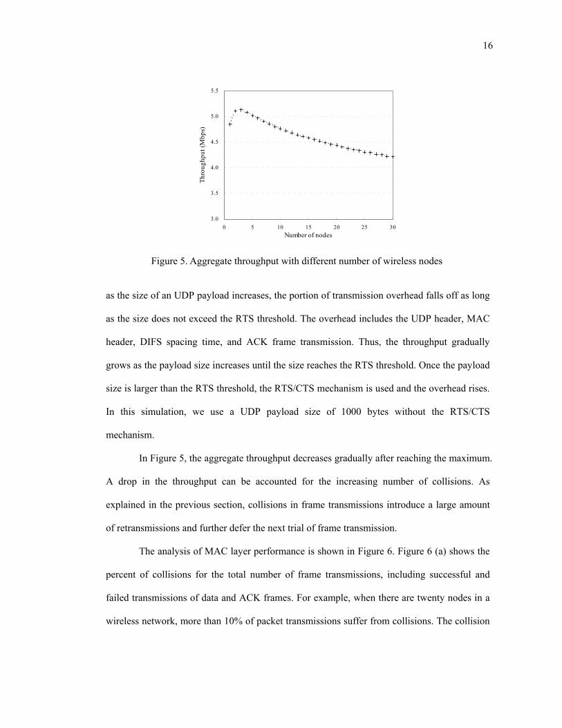
16

as the size of an UDP payload increases, the portion of transmission overhead falls off as long

as the size does not exceed the RTS threshold. The overhead includes the UDP header, MAC

header, DIFS spacing time, and ACK frame transmission. Thus, the throughput gradually

grows as the payload size increases until the size reaches the RTS threshold. Once the payload

size is larger than the RTS threshold, the RTS/CTS mechanism is used and the overhead rises.

In this simulation, we use a UDP payload size of 1000 bytes without the RTS/CTS

mechanism.

In Figure 5, the aggregate throughput decreases gradually after reaching the maximum.

A drop in the throughput can be accounted for the increasing number of collisions. As

explained in the previous section, collisions in frame transmissions introduce a large amount

of retransmissions and further defer the next trial of frame transmission.

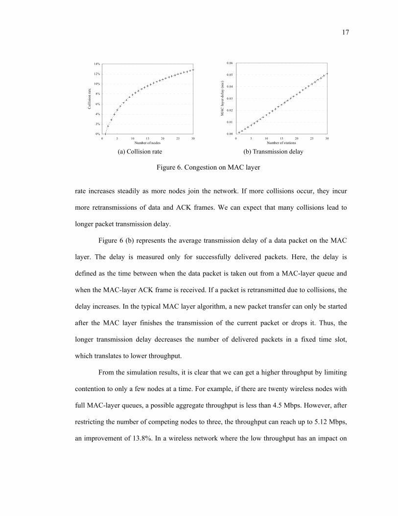
The analysis of MAC layer performance is shown in Figure 6. Figure 6 (a) shows the

percent of collisions for the total number of frame transmissions, including successful and

failed transmissions of data and ACK frames. For example, when there are twenty nodes in a

wireless network, more than 10% of packet transmissions suffer from collisions. The collision

3.0

3.5

4.0

4.5

5.0

5.5

0 5 10 15 20 25 30Number of nodes

Thro

ughp

ut (M

bps)

Figure 5. Aggregate throughput with different number of wireless nodes

17

rate increases steadily as more nodes join the network. If more collisions occur, they incur

more retransmissions of data and ACK frames. We can expect that many collisions lead to

longer packet transmission delay.

Figure 6 (b) represents the average transmission delay of a data packet on the MAC

layer. The delay is measured only for successfully delivered packets. Here, the delay is

defined as the time between when the data packet is taken out from a MAC-layer queue and

when the MAC-layer ACK frame is received. If a packet is retransmitted due to collisions, the

delay increases. In the typical MAC layer algorithm, a new packet transfer can only be started

after the MAC layer finishes the transmission of the current packet or drops it. Thus, the

longer transmission delay decreases the number of delivered packets in a fixed time slot,

which translates to lower throughput.

From the simulation results, it is clear that we can get a higher throughput by limiting

contention to only a few nodes at a time. For example, if there are twenty wireless nodes with

full MAC-layer queues, a possible aggregate throughput is less than 4.5 Mbps. However, after

restricting the number of competing nodes to three, the throughput can reach up to 5.12 Mbps,

an improvement of 13.8%. In a wireless network where the low throughput has an impact on

0%

2%

4%

6%

8%

10%

12%

14%

0 5 10 15 20 25 30Number of nodes

Col

lisio

n ra

te

0.00

0.01

0.02

0.03

0.04

0.05

0.06

0 5 10 15 20 25 30Number of stations

MA

C la

yer d

elay

(sec

)

(a) Collision rate (b) Transmission delay

Figure 6. Congestion on MAC layer

18

performance, this improvement can help applications use network resources more effectively.

It should be noted that scheduling wireless nodes gives a large benefit in terms of

energy consumption. While a node is not scheduled to participate in wireless communication,

the node can be switched to a low-power mode. This reduces power consumption of wireless

nodes. Furthermore, limiting the number of nodes that concurrently access the channel by

scheduling reduces collisions and retransmissions of packets. This also helps in reducing the

power dissipation.

In this section, we examined the performance problem due to contention between the

nodes that are close to each other. Packet collisions by contention happen when multiple nodes

transmit packets during the same backoff slot. In contrast, interference occurs when packet

transmission of other nodes is deferred by a node transmitting data over the channel. In a

large-scale network with multiple cells, nodes in neighboring cells of a transmitting node

suffer from interference from the transmitter. Due to the wide range of carrier sensing, the

effect of interference between cells is a dominating factor of the throughput degradation

problem in multi-cell wireless networks. In the next section we study this interference issue in

detail.

3. Interference in a multi-cell wireless network

Although a single-cell scheduling algorithm successfully reduces contention, it does

not effectively reduce interference in a multi-cell network. This is because it does not consider

interference from nodes in nearby cells. Even if single-cell scheduling reduces contention

from neighboring nodes in the same cell, there is still a large amount of interference from

other nodes in adjacent cells. Thus, active nodes do not have enough chance to access

channels. Moreover, because of location differences, even the nodes in the same cell have

different sets of interfering nodes. This difference often leads to the well-known hidden

19

terminal problem [20].

To explore how much the interference affects the throughput in multi-cell networks,

we run the following simulations. In a multi-cell topology of 533m by 550m size, we locate 39

base stations in a hexagonal pattern. The topology used in this simulation is shown in Figure

19 (a) of Chapter V. The communication range of the radio is set to 50m. The carrier sensing

range is twice as long as the communication range. Therefore, the radio signal of a node

affects nodes in neighboring cells. In this setup, we measure the average throughput and MAC

layer utilization at base stations. MAC layer utilization is defined as how much time the radio

channel has consumed in each of MAC layer state. We focus only on two types of MAC layer

states at base stations; recv, and interference. If a base station is receiving a packet and if the

packet data is not corrupted, it is in a recv state. If a base station fails to receive an

uncorrupted packet because of radio signals from more than one node, the node is in an

interference state. Interference is different from collisions. While collisions are defined as the

coincidental use of a backoff slot by multiple nodes, interference is caused by a hidden

terminal. The other MAC layer states consume a minor portion of simulation time; less than

8% each. Thus, we do not consider the other MAC layer states in this analysis. Data traffic

used in this simulation is UDP upstream from child nodes to the closest base stations. The data

rate from child nodes is set to be higher than the maximum throughput. Therefore, MAC layer

input queues at nodes are always full.

In this simulation, we run only the centralized node-level scheduling algorithm

(CNLS) presented in the next chapter. Briefly, its strategy is to randomly choose a given

number of nodes within a communication range. In the following simulation, we schedule

only four nodes within a communication range. Only the scheduled nodes are allowed to

access the channel. This node-level scheduling reduces packet collisions. Therefore it is very

20

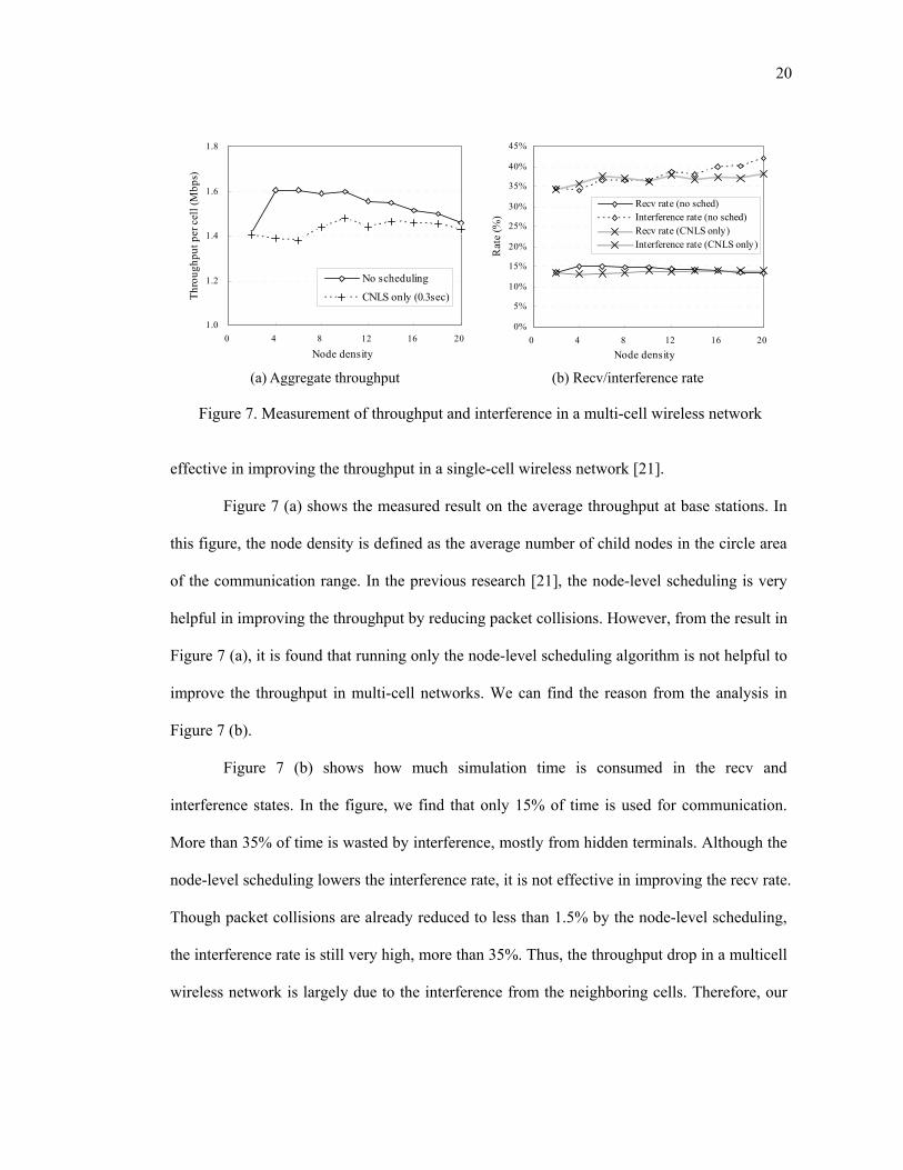
effective in improving the throughput in a single-cell wireless network [21].

Figure 7 (a) shows the measured result on the average throughput at base stations. In

this figure, the node density is defined as the average number of child nodes in the circle area

of the communication range. In the previous research [21], the node-level scheduling is very

helpful in improving the throughput by reducing packet collisions. However, from the result in

Figure 7 (a), it is found that running only the node-level scheduling algorithm is not helpful to

improve the throughput in multi-cell networks. We can find the reason from the analysis in

Figure 7 (b).

Figure 7 (b) shows how much simulation time is consumed in the recv and

interference states. In the figure, we find that only 15% of time is used for communication.

More than 35% of time is wasted by interference, mostly from hidden terminals. Although the

node-level scheduling lowers the interference rate, it is not effective in improving the recv rate.

Though packet collisions are already reduced to less than 1.5% by the node-level scheduling,

the interference rate is still very high, more than 35%. Thus, the throughput drop in a multicell

wireless network is largely due to the interference from the neighboring cells. Therefore, our

1.0

1.2

1.4

1.6

1.8

0 4 8 12 16 20

Node density

Thro

ughp

ut p

er c

ell (

Mbp

s)

No scheduling

CNLS only (0.3sec)

0%

5%

10%

15%

20%

25%

30%

35%

40%

45%

0 4 8 12 16 20Node density

Rat

e (%

)

Recv rate (no sched)Interference rate (no sched)Recv rate (CNLS only)Interference rate (CNLS only)

(a) Aggregate throughput (b) Recv/interference rate

Figure 7. Measurement of throughput and interference in a multi-cell wireless network

21

scheduling algorithm needs to consider both contention within a cell and interference from

neighboring cells.

22

IV. SCHEDULING ALGORITHM

In this chapter, we study an optimal and a heuristic scheduling algorithm for multi-cell

wireless networks, and compare them with our distributed scheduling algorithms. We also

explain our scheduling algorithm in detail.

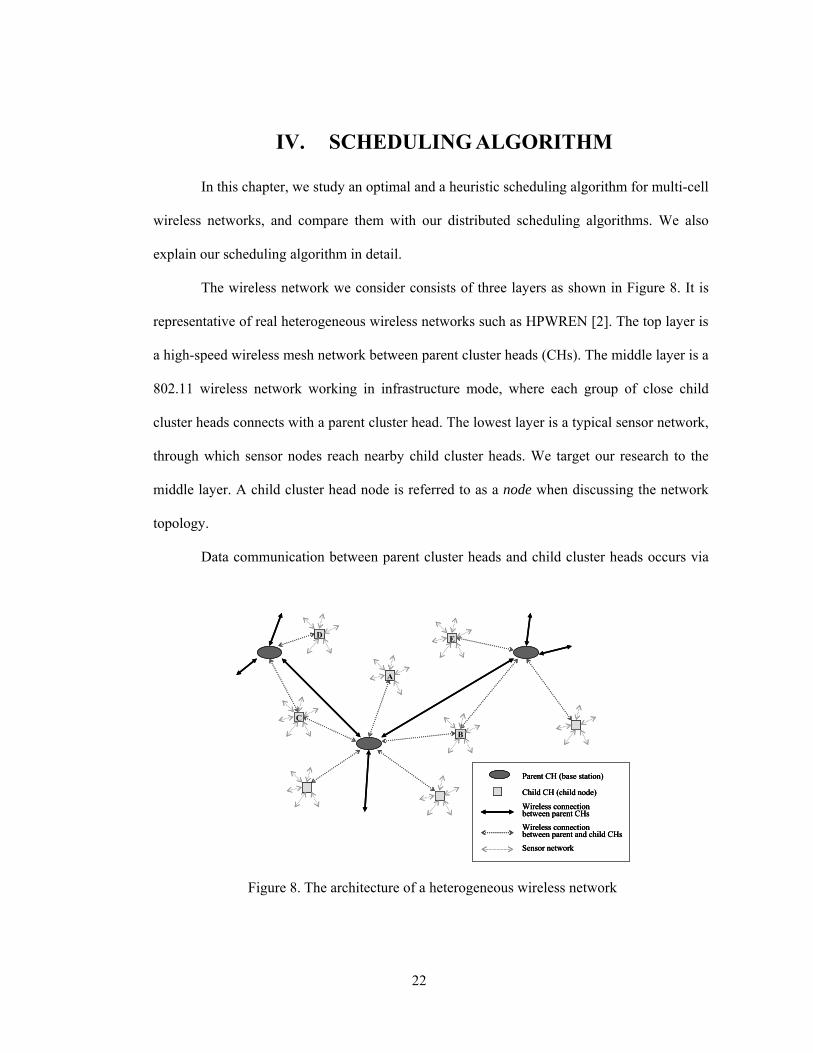
The wireless network we consider consists of three layers as shown in Figure 8. It is

representative of real heterogeneous wireless networks such as HPWREN [2]. The top layer is

a high-speed wireless mesh network between parent cluster heads (CHs). The middle layer is a

802.11 wireless network working in infrastructure mode, where each group of close child

cluster heads connects with a parent cluster head. The lowest layer is a typical sensor network,

through which sensor nodes reach nearby child cluster heads. We target our research to the

middle layer. A child cluster head node is referred to as a node when discussing the network

topology.

Data communication between parent cluster heads and child cluster heads occurs via

C

B

A

D E

Child CH (child node)

Parent CH (base station)

Wireless connectionbetween parent CHs

Wireless connectionbetween parent and child CHs

Sensor network

C

B

A

D E

Child CH (child node)

Parent CH (base station)

Wireless connectionbetween parent CHs

Wireless connectionbetween parent and child CHs

Sensor network

Child CH (child node)

Parent CH (base station)

Wireless connectionbetween parent CHs

Wireless connectionbetween parent and child CHs

Sensor network

Figure 8. The architecture of a heterogeneous wireless network

22

23

the contention-based MAC mechanism. As a result, contention and interferences are issues. To

handle these problems, we first define neighbor nodes as the nodes within communication

range from a target node. Neighbor nodes of Node A can receive the packets from Node A in a

promiscuous mode of the wireless interface. It is possible to get an unique ID for nodes by

reading the source address of packets. Therefore, we assume that a node knows the existence

and the unique node IDs of its neighbor nodes.

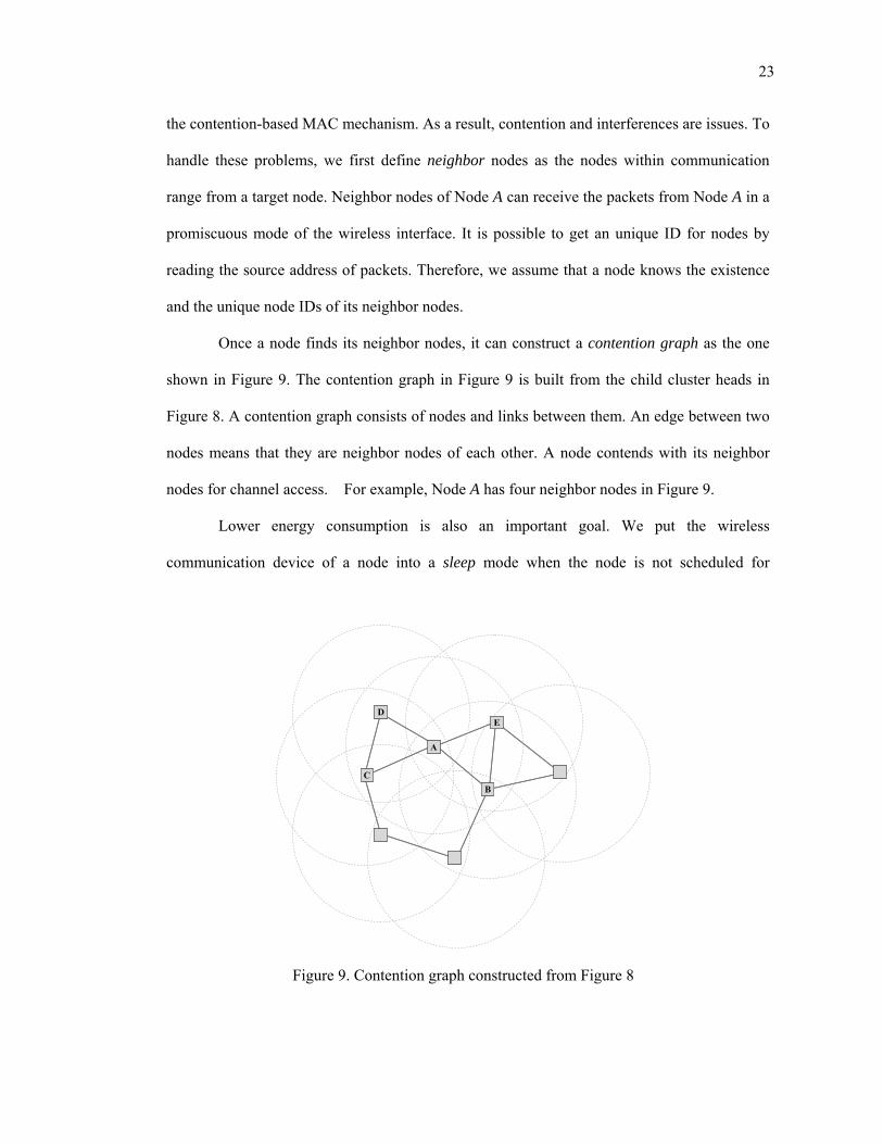
Once a node finds its neighbor nodes, it can construct a contention graph as the one

shown in Figure 9. The contention graph in Figure 9 is built from the child cluster heads in

Figure 8. A contention graph consists of nodes and links between them. An edge between two

nodes means that they are neighbor nodes of each other. A node contends with its neighbor

nodes for channel access. For example, Node A has four neighbor nodes in Figure 9.

Lower energy consumption is also an important goal. We put the wireless

communication device of a node into a sleep mode when the node is not scheduled for

B

E

A

C

D

B

E

A

C

D

Figure 9. Contention graph constructed from Figure 8

24

communication. A node in a sleep mode is called inactive. When an inactive node turns its

wireless interface back to a ready mode, it becomes active. Of course, the mode transition

from the ready mode to the sleep mode or vice versa requires energy higher than in a sleep

mode, as well as the mode transition time.

Our algorithm consists of two parts; cell-level scheduling and node-level scheduling.

These two algorithms schedule active cells and active nodes in scheduled cells respectively.

Once the nodes are scheduled, they are active in the corresponding scheduling interval. The

scheduling interval is a fixed period of time in which a schedule determined by the scheduler

is valid. Our scheduling algorithm is based on a TDMA scheme. At the end of the scheduling

interval, the cell-level scheduling algorithm decides new active cells, and the node-level

scheduling algorithm chooses active nodes in these active cells.

The following sections of this chapter describe our scheduling algorithm in detail. In

the first section, we define the node-level scheduling problem. We show that the optimal

solution for the problem is NP-complete. Because it is very costly to run the algorithm for the

NP-complete problem in a large-scale network at every scheduling time interval, in the next

section we present another heuristic algorithm for the node-level scheduling problem. This

algorithm is then generalized so that it runs in the distributed manner. Finally, we develop a

distributed algorithm that uses both node-level and cell-level scheduling.

1. Optimal node-level scheduling

In this section, we define the node-level scheduling problem. Then we present the

optimal scheduling algorithm for the problem. We also show that the optimal algorithm is

NP-complete. Because it is not practical to repeatedly run an NP-complete algorithm in a

large-scale wireless network, we provide a heuristic solution for the same problem in the next

section.

25

As explained in Section III.2, the wireless MAC suffers from excessive contention

when there are many nodes in a network. The maximum throughput is achieved only when the

number of contending nodes is limited. The node-level scheduling problem in a

contention-based wireless network can then be defined as scheduling at most s nodes in a

given time slot around the contention range of any active node.

Given a network topology of n nodes, we define a contention graph ( )EVG ,= as

shown in Figure 9. A set of vertices V represent the nodes, and a set of edges E represent the

neighbor relationship between the nodes. If a node Vvi ∈ is a neighbor of the other node

Vv j ∈ , then ( ) Evv ji ∈, . The output of a scheduler is an assignment of nodes that are

allowed to access the wireless channel in a given scheduling interval. An active node is a node

which is scheduled to access the wireless channel. Thus, the scheduled assignment is a set of

active nodes AV, where VAV ⊆ .

The main constraint in the node-level scheduling problem is that the number of

neighboring active nodes should not exceed a given constant s. Let ( )ivN be a set of

neighbor nodes of Vvi ∈ . At iv , let the set of active nodes which are in { } ( )ii vNv ∪ be

( )ivAV . In other words, ( )ivAV is a set of active nodes that are either iv or neighbor

nodes of iv . Then, the set of all active nodes in a network is ( )UVv

ii

vAVAV∈

= . In the

constraint definition below, we note that A means the number of elements in the set A.

Constraint : ( ) svAVVv ii ≤∈∀ , where ( )ivAV is the number of

nodes in ( )ivAV - I.1

In scheduling wireless networks, the optimal schedule assigns active nodes such that

26

the assignment maximizes the size of AV . This assignment is called maximum assignment.

In terms of the number of active nodes in a given network, maximum assignment is optimal.

On the other hand, maximal assignment is to schedule the nodes so that the number of active

nodes is maximal. By maximal we mean that no additional assignment of an active node to an

existing schedule can meet Constraint I.1. The maximal assignment problem is simpler than

the maximum assignment and it can be solved in polynomial time. The output of maximal

assignment is dependent on the order of scheduled nodes. The number of active nodes in a

maximal assignment is equal to or less than that of a maximum assignment.

It has been shown in [5] and [9] that the maximum assignment problem for s = 1 is

NP-complete. Maximal assignment requires less computation than the maximum scheduling.

We show that the maximum assignment problem for s > 1 is also NP-complete. We argue that

scheduling the maximal assignment of nodes is feasible for scalable wireless networks.

NP completeness of the maximum assignment for s = 1

It has been reported in [9] that the decision problem of whether there exists an

assignment of t active nodes in a given network is equivalent to the maximum clique problem,

which is an NP-complete problem. We briefly summarize it here.

In a network graph ( )EVG ,= and a set of scheduled active nodes VAV ⊆ , any

two adjacent nodes cannot be active at the same time because s = 1. In other words, if a node

is active, all its neighboring nodes cannot be active.

{ } AVvv ji ⊄, if ji ≠ and ( ) Evv ji ∈,

We map a graph ( )EVG ,= into the corresponding ( )EVG ′′=′ , as the following.

27

Vertices : VV ←′

Edges : ( ){ }ji vvEE ,∪′←′ for ji,∀ where ji ≠ and ( ) Evv ji ∉,

G′ has the same nodes as G . Nodes iv and jv in G′ have an edge between

them if and only if iv and jv are not a neighbor node of each other in G . Then, the

decision problem of scheduling t active nodes in G is equivalent to the problem of finding a

clique of size t in G′ . There exists one-to-one mapping between G and G′ . The mapping

takes polynomial time. The decision problem of maximum clique is known as NP-complete.

Therefore, finding the maximum assignment for s = 1 is NP-complete.

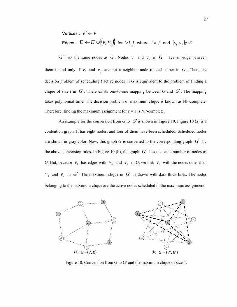
An example for the conversion from G to G′ is shown in Figure 10. Figure 10 (a) is a

contention graph. It has eight nodes, and four of them have been scheduled. Scheduled nodes

are shown in gray color. Now, this graph G is converted to the corresponding graph G′ by

the above conversion rules. In Figure 10 (b), the graph G′ has the same number of nodes as

G. But, because 1v has edges with 4v and 7v in G, we link 1v with the nodes other than

4v and 7v in G′ . The maximum clique in G′ is drawn with dark thick lines. The nodes

belonging to the maximum clique are the active nodes scheduled in the maximum assignment.

7

2

1

3

8

4

5

6

7

2

1

3

8

4

5

6

7

2

1

3

8

4

5

6

7

2

1

3

8

4

5

6

(a) ( )EVG ,= (b) ( )EVG ′′=′ ,

Figure 10. Conversion from G to G’ and the maximum clique of size 4.

28

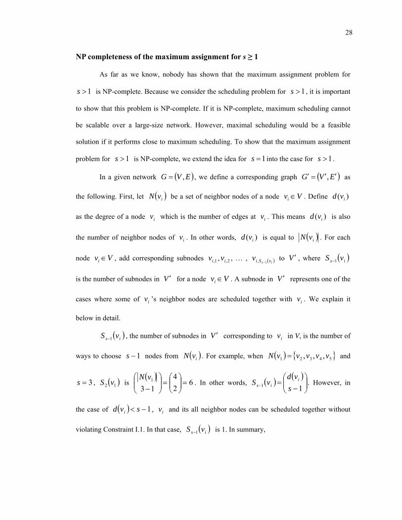
NP completeness of the maximum assignment for s ≥ 1

As far as we know, nobody has shown that the maximum assignment problem for

1>s is NP-complete. Because we consider the scheduling problem for 1>s , it is important

to show that this problem is NP-complete. If it is NP-complete, maximum scheduling cannot

be scalable over a large-size network. However, maximal scheduling would be a feasible

solution if it performs close to maximum scheduling. To show that the maximum assignment

problem for 1>s is NP-complete, we extend the idea for 1=s into the case for 1>s .

In a given network ( )EVG ,= , we define a corresponding graph ( )EVG ′′=′ , as

the following. First, let ( )ivN be a set of neighbor nodes of a node Vvi ∈ . Define )( ivd

as the degree of a node iv which is the number of edges at iv . This means )( ivd is also

the number of neighbor nodes of iv . In other words, )( ivd is equal to ( )ivN . For each

node Vvi ∈ , add corresponding subnodes 1,iv , 2,iv , … , ( )is vSiv1, −

to V ′ , where ( )is vS 1−

is the number of subnodes in V ′ for a node Vvi ∈ . A subnode in V ′ represents one of the

cases where some of iv ’s neighbor nodes are scheduled together with iv . We explain it

below in detail.

( )is vS 1− , the number of subnodes in V ′ corresponding to iv in V, is the number of

ways to choose 1−s nodes from ( )ivN . For example, when ( ) { }54321 ,,, vvvvvN = and

3=s , ( )12 vS is ( )

624

131 =⎟⎟

⎠

⎞⎜⎜⎝

⎛=⎟⎟

⎠

⎞⎜⎜⎝

⎛−vN

. In other words, ( ) ( )⎟⎟⎠

⎞⎜⎜⎝

⎛−

=− 11 svd

vS iis . However, in

the case of ( ) 1−< svd i , iv and its all neighbor nodes can be scheduled together without

violating Constraint I.1. In that case, ( )is vS 1− is 1. In summary,

29

( )is vS 1− is, ( )

⎟⎟⎠

⎞⎜⎜⎝

⎛−1svd i if ( ) 1−≥ svd i , or 1 if ( ) 1−< svd i - I.2

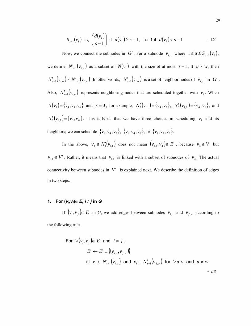
Now, we connect the subnodes in G′ . For a subnode uiv , where ( )is vSu 11 −≤≤ ,

we define ( )uis vN ,1−′ as a subset of ( )ivN with the size of at most 1−s . If wu ≠ , then

( ) ( )wisuis vNvN ,1,1 −− ′≠′ . In other words, ( )uis vN ,1−′ is a set of neighbor nodes of uiv , in G′ .

Also, ( )uis vN ,1−′ represents neighboring nodes that are scheduled together with iv . When

( ) { }6541 ,, vvvvN = and 3=s , for example, ( ) { }541,12 ,vvvN =′ , ( ) { }642,12 ,vvvN =′ , and

( ) { }653,12 ,vvvN =′ . This tells us that we have three choices in scheduling 1v and its

neighbors; we can schedule { }541 ,, vvv , { }641 ,, vvv , or { }651 ,, vvv .

In the above, ( )1,114 vNv ′∈ does not mean ( ) Evv ′∈41,1 , , because Vv ∈4 but

Vv ′∈1,1 . Rather, it means that 1,1v is linked with a subset of subnodes of 4v . The actual

connectivity between subnodes in V ′ is explained next. We describe the definition of edges

in two steps.

1. For (vi,vj)∈E, i≠ j in G

If ( ) Evv ji ∈, in G, we add edges between subnodes uiv , and wjv , according to

the following rule.

For ( ) Evv ji ∈∀ , and ji ≠ ,

( ){ }wjui vvEE ,, ,∪′←′

iff ( )uisj vNv ,1−′∈ and ( )wjsi vNv ,1−′∈ for vu,∀ and wu ≠

- I.3

30

For example, in Figure 11, 1v has an edge with 5v in G. 1v has two subnodes

1,1v and 2,1v in G′ . 5v also has two subnodes 1,5v and 2,5v . Because s = 2, if a node is

scheduled, we can schedule at most one of its neighbor node. So, ( ) { }41,11 vvN s =′− and

( ) { }52,11 vvN s =′− . In the same way, ( ) { }11,51 vvN s =′− and ( ) { }42,51 vvN s =′− . Now, we find

that ( )2,115 vNv s−′∈ and ( )1,511 vNv s−′∈ . Therefore, we place an edge between 2,1v and

1,5v by Rule I.3. The edges created by Rule I.3 are drawn with dashed lines in Figure 11.

2. For (vi,vj)∉E, i≠ j in G

( ) Evv ji ∉, means that iv and jv are not neighbor of each other. In this case, all

subnodes of iv can have links to subnodes of jv . We can do this conversion by adding Rule

I.4 to the definition of ( )uis vN ,1−′ . Subnodes of iv are then linked to subnodes of jv by

Rule I.3.

2

1

3

4

5

2

1

3

4

5

3,1

5,2

1,1

2,1

4,14,2

4,34,4

5,1

1,2

3,22,2 3,1

5,2

1,1

2,1

4,14,2

4,34,4

5,1

1,2

3,22,2

(a) ( )EVG ,= (b) ( )EVG ′′=′ ,

Figure 11. Conversion from G to G′ , for s = 2

31

For ( ) Evv ji ∈∀ , and ji ≠ ,

( ) ( ) { }juisuis vvNvN ∪′←′ −− ,1,1 and ( ) ( ) { }iwjswjs vvNvN ∪′←′ −− ,1,1

for vu,∀ and wu ≠ - I.4

Rule I.4 means that any node jv in G is added to ( )uis vN ,1−′ if jv is neither iv

itself nor a neighbor node of iv in G. For example, in Figure 11, 2v and 3v are not

neighbor nodes of 1v . So, 2v and 3v are added to both ( )1,11 vN s−′ and ( )2,11 vN s−′ . The

edges created by Rule I.4 are drawn as solid lines.

When 2=s , the maximum assignment in Figure 11 is to schedule 4 nodes. We color

the scheduled nodes as gray. Figure 11 (b) is a graph converted from Figure 11 (a). The

maximum clique is shown with thick black lines. The size of a maximum clique is 4, so we

can schedule up to four nodes.

Let the maximum clique found in G′ be ( ) ),( MEMVGMC =′ . Then, we can

derive the following facts from ( )GMC ′ :

Lemma 1 : If MVv ui ∈, , then MVv wi ∉, for wu ≠∀ - I.5

Let us suppose that MVv ui ∈, and MVv wi ∈, for wu ≠ . Then, there must be

( ) Evv wiui ′∈,, , , because ( )GMC ′ is a maximum clique in G′ . In a clique, there exist

edges between all pairs of nodes. However, by the definition of a subnode and by Rule I.3 and

Rule I.4, there cannot be any edges between subnodes derived from the same node. Therefore,

( )GMC ′ includes at most one subnode for a node Vvi ∈ .

32

Lemma 2 : - I.6

If there is a schedulable assignment of nodes in G ,

there exists a corresponding clique in G′ .

When a given assignment of nodes is schedulable, it means ( ) svAV i ≤ for

AVvi ∈∀ . It is obvious that ( ) { } svvAV ii <− at any active node AVvi ∈ . By the

definition of ( )uik vN ,1−′ , there must be at least one subnode uiv , satisfying

( ) { } ( )uikii vNvvAV ,1−′⊂− . It is because subnodes of iv cover all combinations of having

1−s neighbor nodes of iv ’s neighbors.

By the above, when two active nodes iv and jv satisfy ( )ij vNv ∈ , it is always

true that there exists a subnode uiv , of iv and a subnode wjv , of jv satisfying

( ) Evv wjui ′∈,, , . For iv and jv , if ( )ij vNv ∉ , then every subnode of iv has edges with

every subnode of jv in G′ by Rule I.4. Therefore, whenever a schedulable assignment of

nodes is given in G , there exists a corresponding clique in G′ .

Lemma 3 : - I.7

If there is a clique in G′ , there is a corresponding assignment of nodes in G .

By Lemma 1, the clique has at most one subnode for each Vvi ∈ . By the definition

of Rule I.3 and of a maximum clique, a subnode MVv ui ∈, has at most 1−s edges in

( )GMC ′ with the subnodes of ( )ivN . So, any node Vvi ∈ corresponding to MVv ui ∈,

does not violate Constraint I.1.

The assignment of nodes corresponding to ( )GMC ′ is just to schedule the nodes

33

corresponding to MV ; for example, a schedule iv if MVv ui ∈, for any subnode uiv , of

iv . Obviously, the conversion from ( )GMC ′ into the assignment in G takes ( )VO time.

Lemma 4 : Conversion of G into G′ takes polynomial time. - I.8

Finding ( )ivN for all Vvi ∈ takes ( )EVO ⋅ time. Rule I.3 takes ( )EVO ⋅

time, and Rule I.4 needs ( )2EVO ⋅ time. Therefore, the conversion from G to G′ takes

polynomial time.

Theorem : The maximum scheduling problem is NP-complete. - I.9

By Lemma 2 and 3, there is an one-to-one mapping between the schedulable

assignments in G and maximum cliques in G′ . By Lemma 4, the conversion of a given

network G to G′ takes polynomial time. As shown in Lemma 3, it also takes polynomial

time to map a maximum clique in G′ into the schedulable assignment in G . We know that

the maximum clique problem is NP-complete. Therefore, the given scheduling problem is-NP

complete.

The goal of maximum scheduling is to maximize the number of scheduled nodes. On

the other hand, maximal scheduling aims to schedule nodes until no more nodes can be

scheduled. We showed that maximal scheduling problem is equivalent to the maximum clique

problem which is known to be NP-complete. Running an NP-complete scheduling algorithm

at every scheduling interval causes excessive runtime overhead. Therefore, in this research, we

use maximal scheduling as a solution for determining the node-level schedule in a multi-cell

wireless network. In the following sections, we present the centralized algorithm for maximal

node-level scheduling. We next derive the distributed algorithm from the centralized version.

34

2. Centralized node-level scheduling (CNLS)

In this section, we first review the maximal node-level scheduling of a multi-cell

wireless network for the case of ( 1=s ) where s is the maximum number of contending active

nodes in a communication range. The algorithm for 1=s has been presented in [9]. As

explained in Section III.2 and III.3, we can achieve additional throughput gain and better

utilization of radio channels by scheduling more than one node at a time. Furthermore, we

extend the solution for 1=s to the case of scheduling for 1>s in a latter part of this

section. We also note that the node-level scheduling algorithms presented in this section and

the next section use a pseudo-random numbers generated with a seed value of node ID.

Therefore, it is possible for each node to generate the identical set of pseudo-random values

for all nodes. This eliminates runtime overhead of distributing a schedule to remote nodes at

every scheduling interval.

Maximal assignment provides a deterministic node-level schedule when the network

topology is known in advance. By deterministic, we mean that the algorithm for maximal

assignment always gives the same assignment of active nodes if the order of pseudo-random

numbers is fixed. Because the algorithm requires the complete knowledge of network

topology, we say that this algorithm runs in a centralized manner. In contrast, the distributed

node-level scheduling presented in the next section gives maximal assignment only with the

knowledge of local topology. Therefore, it is possible for each node to run the distributed

node-level scheduling algorithm. We first study the centralized node-level scheduling in this

section, and convert it into a distributed version in the next section.

The centralized node-level scheduling algorithm (CNLS) for maximal scheduling

based on [9] is shown in Algorithm I.10. The algorithm first chooses a node from vertices V,

and schedules the node to the assignment of active nodes. Then the scheduled node and its

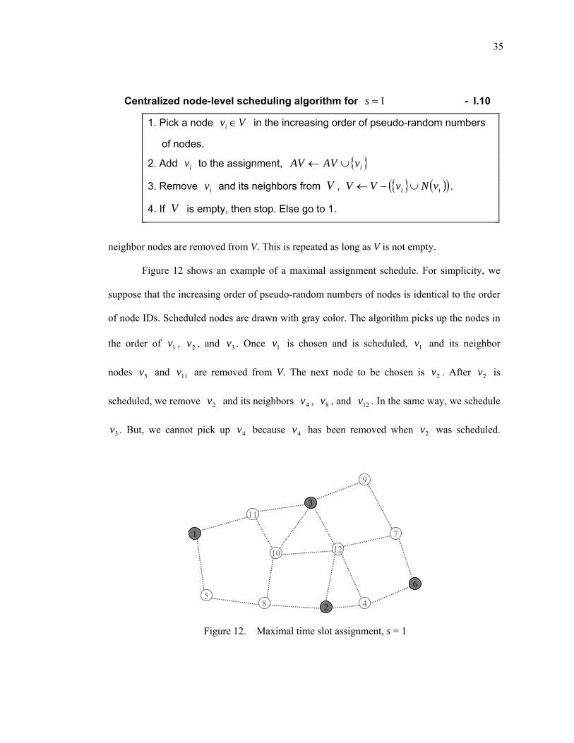
35

neighbor nodes are removed from V. This is repeated as long as V is not empty.

Figure 12 shows an example of a maximal assignment schedule. For simplicity, we

suppose that the increasing order of pseudo-random numbers of nodes is identical to the order

of node IDs. Scheduled nodes are drawn with gray color. The algorithm picks up the nodes in

the order of 1v , 2v , and 3v . Once 1v is chosen and is scheduled, 1v and its neighbor

nodes 5v and 11v are removed from V. The next node to be chosen is 2v . After 2v is

scheduled, we remove 2v and its neighbors 4v , 8v , and 12v . In the same way, we schedule

3v . But, we cannot pick up 4v because 4v has been removed when 2v was scheduled.

Centralized node-level scheduling algorithm for 1=s - I.10

1. Pick a node Vvi ∈ in the increasing order of pseudo-random numbers

of nodes.

2. Add iv to the assignment, { }ivAVAV ∪←

3. Remove iv and its neighbors from V , { } ( )( )ii vNvVV ∪−← .

4. If V is empty, then stop. Else go to 1.

7

11

25

1

3

9

6

1210

48

7

11

25

1

3

9

6

1210

48

Figure 12. Maximal time slot assignment, s = 1

36

Hence, we choose the next available node 6v . After 6v is scheduled, there is no more node

to choose. Then, the algorithm terminates.

We next consider the case with more than one contending nodes within

communication ranges (s > 1). In Algorithm I.10, the scheduled node iv and its neighbors

( )ivN are deleted from a node set V because both iv and its neighbors already have one

active node in their communication range. To guarantee the schedule to the case of

( ) 1>ivAV , we assign s tickets to each node. The number of initial tickets in each node is

equal to a constant s given in a scheduling constraint. The number of tickets at iv limits

( )ivAV , the maximum number of active nodes at iv . In this way, we limit the number of

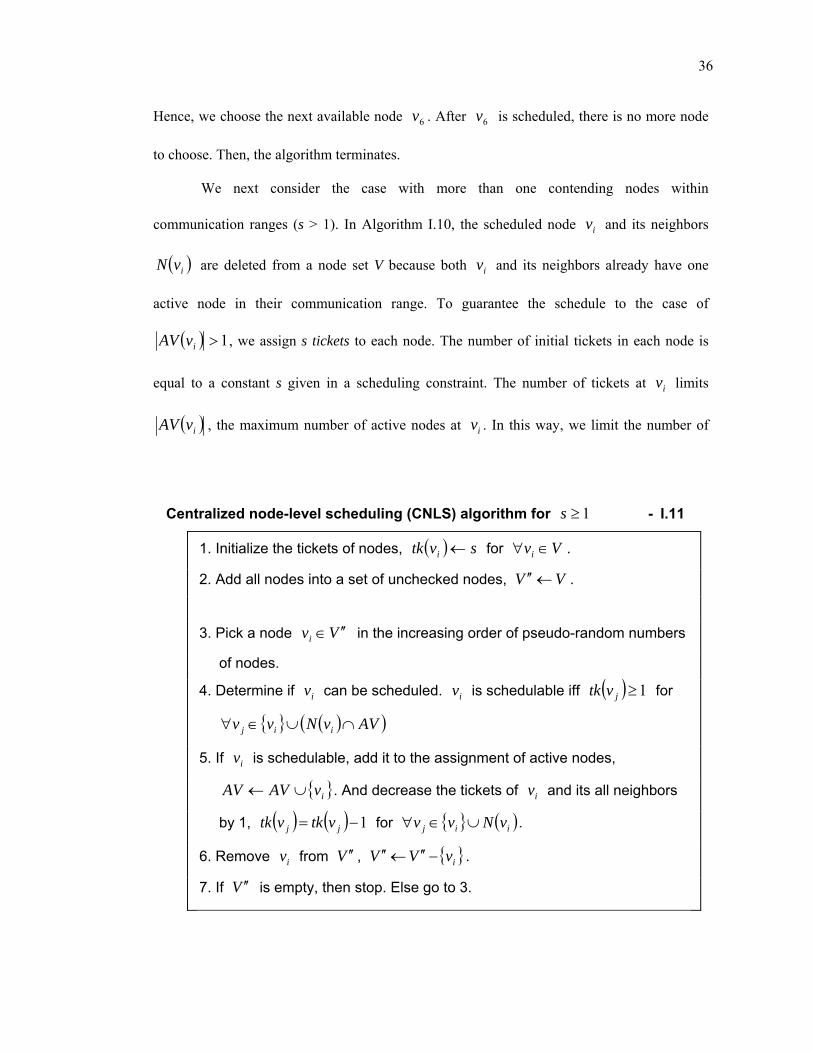
Centralized node-level scheduling (CNLS) algorithm for 1≥s - I.11

1. Initialize the tickets of nodes, ( ) svtk i ← for Vvi ∈∀ .

2. Add all nodes into a set of unchecked nodes, VV ←′′ .

3. Pick a node Vvi ′′∈ in the increasing order of pseudo-random numbers

of nodes.

4. Determine if iv can be scheduled. iv is schedulable iff ( ) 1≥jvtk for

{ } ( )( )AVvNvv iij ∩∪∈∀

5. If iv is schedulable, add it to the assignment of active nodes,

{ }ivAVAV ∪← . And decrease the tickets of iv and its all neighbors

by 1, ( ) ( ) 1−= jj vtkvtk for { } ( )iij vNvv ∪∈∀ .

6. Remove iv from V ′′ , { }ivVV −′′←′′ .

7. If V ′′ is empty, then stop. Else go to 3.

37

contending nodes. For example, if a node has three tickets, we can schedule up to three nodes

from the node and its neighbors. Let the current number of ticket at iv be ( )ivtk . Note that

( )ivtk may be negative if iv is not scheduled in a given scheduling interval. Whenever the

algorithm runs at every scheduling interval, ( )ivtk is initialized as ( ) svtk i = . The new

algorithm is shown in Algorithm I.11.

The new algorithm initially allocates s tickets to all nodes. If the number of active

nodes near an unscheduled node iv is equal to or greater than s, the number of tickets at iv

cannot be greater than zero, ( ) 1<ivtk . Therefore, we do not schedule iv because iv already

consumed its tickets. Otherwise, iv is scheduled. In either case, we remove iv from V ′′ . The

algorithm terminates if there is no more node to pick up from V ′′ . By step 4 of Algorithm I.11,

the new algorithm guarantees that, at any active node, the number of active nodes does not

exceed the given constant s.

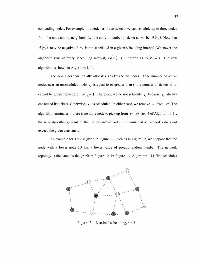
An example for s = 2 is given in Figure 13. Such as in Figure 12, we suppose that the

node with a lower node ID has a lower value of pseudo-random number. The network

topology is the same as the graph in Figure 12. In Figure 13, Algorithm I.11 first schedules

7

11

2

1

3

9

6

12

8 45

10

7

11

2

1

3

9

6

12

8 45

10

Figure 13. Maximal scheduling, s = 2

38

1v . After 1v is scheduled, the number of tickets at 1v , 5v , and 11v is decreased by 1. As a

result, we get ( ) 11 =vtk , ( ) 15 =vtk , and ( ) 111 =vtk . In the same way, 2v , 3v , 4v , and

5v are scheduled. When we try to schedule 6v , we find that one of active neighbor nodes of

6v has no remaining ticket, ( ) 04 =vtk . Hence, 6v cannot be scheduled. However, 6v can

be scheduled even if the neighbor node 12v has no ticket, ( ) 012 =vtk . We only look at the

number of tickets only at active nodes. In addition, It is obvious that when 1=s , the CNLS

algorithm in I.11 is identical to Algorithm I.10. Therefore we can say that Algorithm I.11 is

valid for 1≥s .

CNLS algorithm gives a maximal scheduling when the whole topology of a network is

known. However, maintaining the topology information at every node will result in a lot of

overhead at runtime. As the network grows into a large in scale, the size of the topology

information and the execution time of algorithm will also increase. Therefore, we need to run

the CNLS algorithm in a distributed manner. By distributed, we mean that each node runs the

node-level scheduling algorithm on its own in order to decide its schedule at every scheduling

interval. We present a distributed version of CNLS in the next section. The performance of

both scheduling algorithms is analyzed in Chapter V.

3. Distributed node-level scheduling (DNLS)

In this section, we present a distributed node-level scheduling (DNLS) algorithm for

maximal scheduling. The CNLS algorithm in Algorithm I.11 of the previous section runs with

the knowledge of the whole network topology. In a practical wireless network, however, it is

not easy to share the complete network topology among all wireless nodes in a network. To

update the topology information at all nodes whenever a new node joins the network requires

high overhead in running-time and communication. Running the CNLS algorithm at every

39

node is also redundant. Each node is interested only in its own schedule. Our distributed

node-level scheduling algorithm addresses all these issues.

We first define the input to the distributed algorithm. In the centralized algorithm

(Algorithm I.11), its input is the network topology; a contention graph. In a distributed

scheduling algorithm which we present here, we use a partial knowledge of the network

topology. We call this partial network topology a subnetwork. The size of a subnetwork is an

important factor in determining accuracy and efficiency of our DNLS algorithm. For example,

let us think of running DNLS with a subnetwork of one hop distance nodes. Each node runs

Algorithm I.11 only for a subnetwork that includes the node itself and its neighbor nodes.

However, because the schedule of a node is dependent on the schedule of its neighbor nodes,

we cannot guarantee that the schedule resulting from the knowledge of subnetwork is always

consistent with the result of the original CNLS for a total network. On the other hand,

increasing the size of a subnetwork creates large overhead at runtime. Even a small change in

the network topology propagates to a number of nodes, and the overhead increases

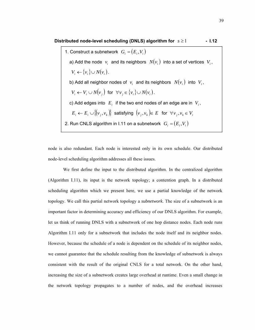
Distributed node-level scheduling (DNLS) algorithm for 1≥s - I.12

1. Construct a subnetwork ( )iii VEG ,=

a) Add the node iv and its neighbors ( )ivN into a set of vertices iV ,

{ } ( )iii vNvV ∪← .

b) Add all neighbor nodes of iv and its neighbors ( )ivN into iV ,

( )jii vNVV ∪← for { } ( )iij vNvv ∪∈∀ .

c) Add edges into iE if the two end nodes of an edge are in iV ,

( ){ }kjii vvEE ,∪← satisfying ( ) Evv kj ∈, for ikj Vvv ∈∀ ,

2. Run CNLS algorithm in I.11 on a subnetwork ( )iii VEG ,=

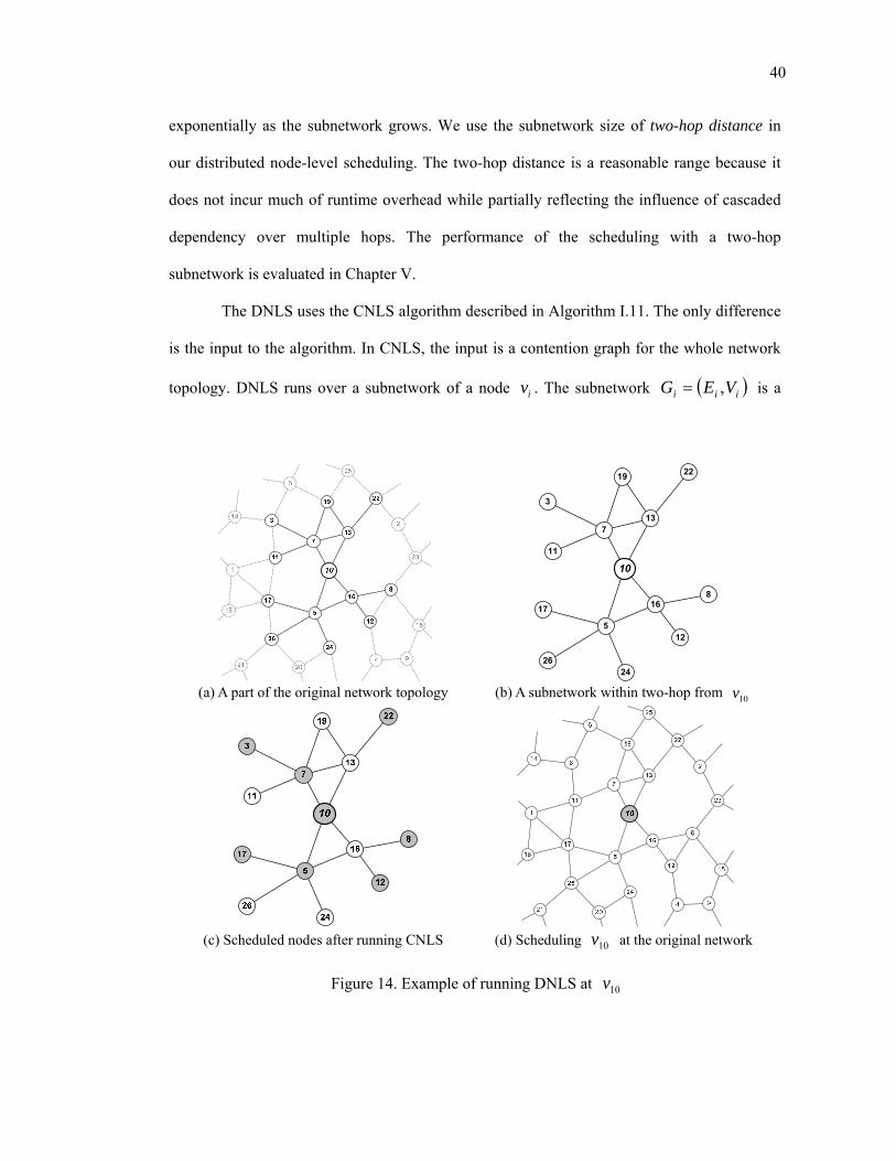
40

exponentially as the subnetwork grows. We use the subnetwork size of two-hop distance in

our distributed node-level scheduling. The two-hop distance is a reasonable range because it

does not incur much of runtime overhead while partially reflecting the influence of cascaded

dependency over multiple hops. The performance of the scheduling with a two-hop

subnetwork is evaluated in Chapter V.

The DNLS uses the CNLS algorithm described in Algorithm I.11. The only difference

is the input to the algorithm. In CNLS, the input is a contention graph for the whole network

topology. DNLS runs over a subnetwork of a node iv . The subnetwork ( )iii VEG ,= is a

10

7

26

12

13

8

11

5

3

17 16

19 22

24 (a) A part of the original network topology (b) A subnetwork within two-hop from 10v

(c) Scheduled nodes after running CNLS (d) Scheduling 10v at the original network

Figure 14. Example of running DNLS at 10v

41

subset of ( )EVG ,= . All vertices and edges within two hops distance from iv are added to

the subnetwork ( )iii VEG ,= . Once a subnetwork is created, we run the CNLS algorithm

only on this subnetwork. The result of the CNLS algorithm becomes the schedule of iv . We

present the DNLS algorithm in I.12. At the last step of I.12, the schedule of iv is determined

by running CNLS algorithm on ( )iii VEG ,= .

Figure 14 shows an example of constructing a subnetwork and running the DNLS at a

node 10v . In Figure 14 (a), the node 10v has four one-hop neighbor nodes and nine two-hop

neighbor nodes. We build a subnetwork consisting of 14 nodes in Figure 14 (b). This is a

subnetwork ( )101010 ,VEG = for a node 10v . Next, we run the CNLS algorithm over this

subnetwork. The result is shown in Figure 14 (c). Since we run this scheduling algorithm at

10v , we are interested only in the schedule of 10v . The result from running CNLS over the

subnetwork says that 10v is scheduled. Thus, DNLS algorithm gives the result that 10v is

scheduled. The DNLS algorithm is repeated by all nodes at every scheduling interval.

The distributed node-level scheduling algorithm for a maximal scheduling has been

presented in this section. The DNLS algorithm runs over a subnetwork that is a part of the

whole network topology. As each node needs to know of nodes within two-hops distance, the

DNLS algorithm reduces a large amount of computational complexity and runtime overhead

in communication. Therefore, we use DNLS algorithm as a node-level scheduling algorithm.

In the next section, we consider the cell-level scheduling algorithm. In our complete

scheduling algorithm, the node-level scheduling algorithm is combined with the cell-level

scheduling algorithm.

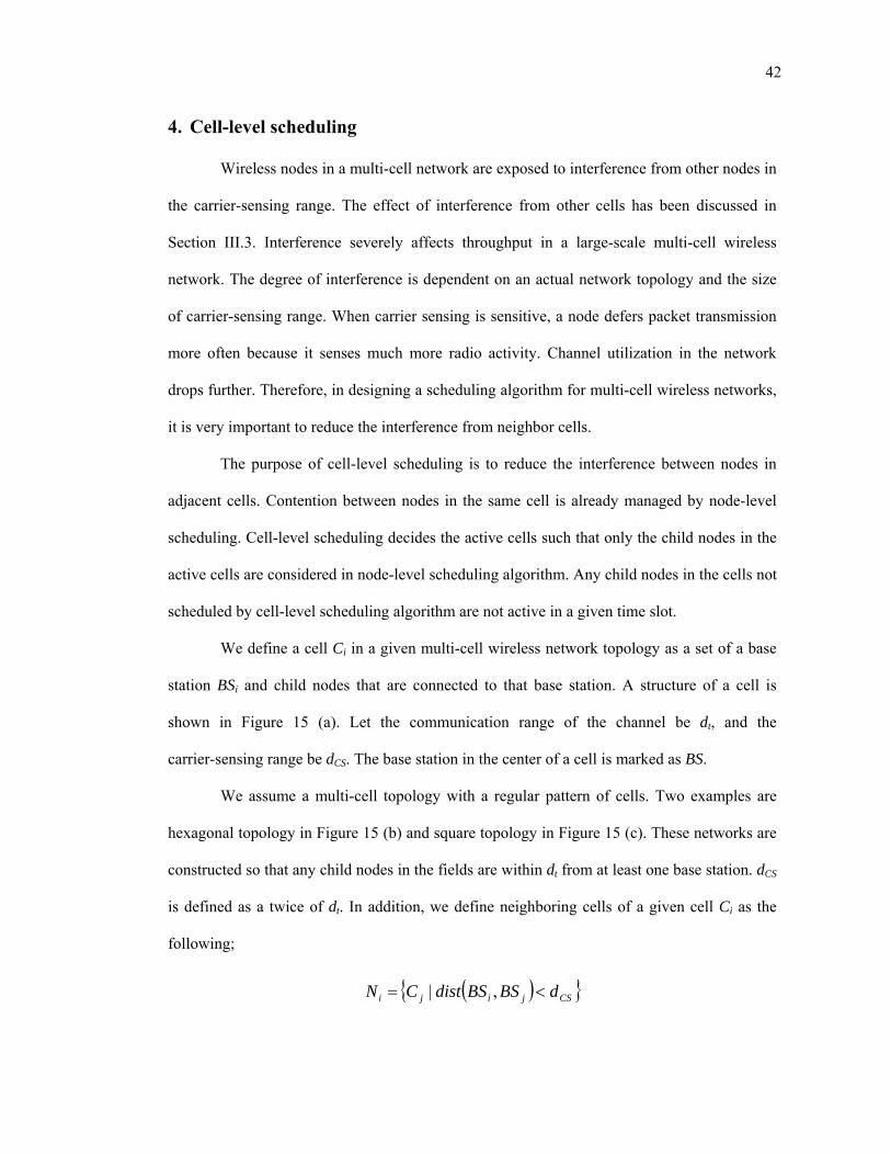
42

4. Cell-level scheduling

Wireless nodes in a multi-cell network are exposed to interference from other nodes in

the carrier-sensing range. The effect of interference from other cells has been discussed in

Section III.3. Interference severely affects throughput in a large-scale multi-cell wireless

network. The degree of interference is dependent on an actual network topology and the size

of carrier-sensing range. When carrier sensing is sensitive, a node defers packet transmission

more often because it senses much more radio activity. Channel utilization in the network

drops further. Therefore, in designing a scheduling algorithm for multi-cell wireless networks,

it is very important to reduce the interference from neighbor cells.

The purpose of cell-level scheduling is to reduce the interference between nodes in

adjacent cells. Contention between nodes in the same cell is already managed by node-level

scheduling. Cell-level scheduling decides the active cells such that only the child nodes in the

active cells are considered in node-level scheduling algorithm. Any child nodes in the cells not

scheduled by cell-level scheduling algorithm are not active in a given time slot.

We define a cell Ci in a given multi-cell wireless network topology as a set of a base

station BSi and child nodes that are connected to that base station. A structure of a cell is

shown in Figure 15 (a). Let the communication range of the channel be dt, and the

carrier-sensing range be dCS. The base station in the center of a cell is marked as BS.

We assume a multi-cell topology with a regular pattern of cells. Two examples are

hexagonal topology in Figure 15 (b) and square topology in Figure 15 (c). These networks are

constructed so that any child nodes in the fields are within dt from at least one base station. dCS

is defined as a twice of dt. In addition, we define neighboring cells of a given cell Ci as the

following;

( ){ }CSjiji dBSBSdistCN <= ,|

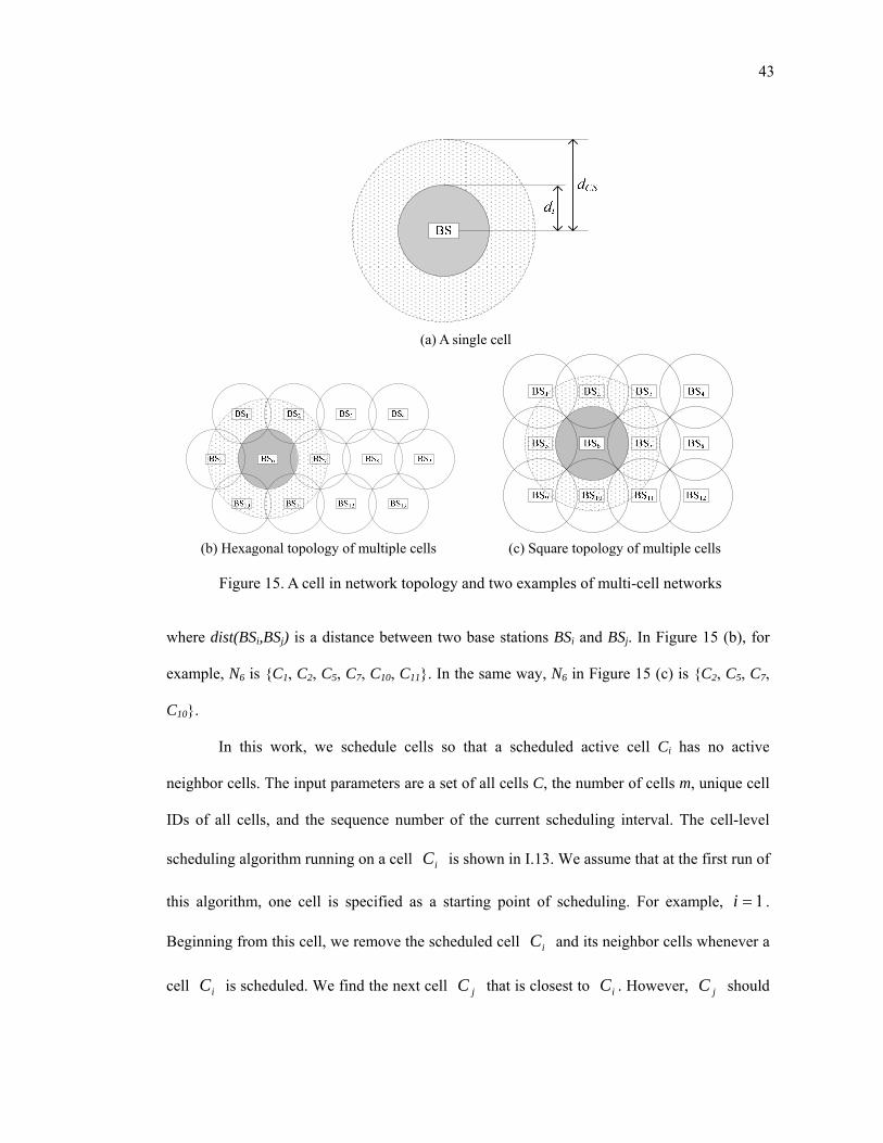
43

where dist(BSi,BSj) is a distance between two base stations BSi and BSj. In Figure 15 (b), for

example, N6 is {C1, C2, C5, C7, C10, C11}. In the same way, N6 in Figure 15 (c) is {C2, C5, C7,

C10}.

In this work, we schedule cells so that a scheduled active cell Ci has no active

neighbor cells. The input parameters are a set of all cells C, the number of cells m, unique cell

IDs of all cells, and the sequence number of the current scheduling interval. The cell-level

scheduling algorithm running on a cell iC is shown in I.13. We assume that at the first run of

this algorithm, one cell is specified as a starting point of scheduling. For example, 1=i .

Beginning from this cell, we remove the scheduled cell iC and its neighbor cells whenever a

cell iC is scheduled. We find the next cell jC that is closest to iC . However, jC should

(a) A single cell

(b) Hexagonal topology of multiple cells (c) Square topology of multiple cells

Figure 15. A cell in network topology and two examples of multi-cell networks

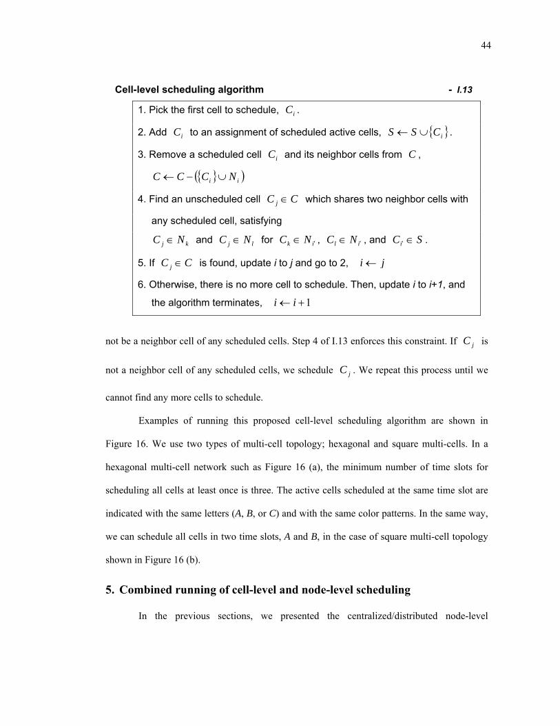
44

not be a neighbor cell of any scheduled cells. Step 4 of I.13 enforces this constraint. If jC is

not a neighbor cell of any scheduled cells, we schedule jC . We repeat this process until we

cannot find any more cells to schedule.

Examples of running this proposed cell-level scheduling algorithm are shown in

Figure 16. We use two types of multi-cell topology; hexagonal and square multi-cells. In a

hexagonal multi-cell network such as Figure 16 (a), the minimum number of time slots for

scheduling all cells at least once is three. The active cells scheduled at the same time slot are

indicated with the same letters (A, B, or C) and with the same color patterns. In the same way,

we can schedule all cells in two time slots, A and B, in the case of square multi-cell topology

shown in Figure 16 (b).

5. Combined running of cell-level and node-level scheduling

In the previous sections, we presented the centralized/distributed node-level

Cell-level scheduling algorithm - I.13

1. Pick the first cell to schedule, iC .

2. Add iC to an assignment of scheduled active cells, { }iCSS ∪← .

3. Remove a scheduled cell iC and its neighbor cells from C ,

{ }( )ii NCCC ∪−←

4. Find an unscheduled cell CC j ∈ which shares two neighbor cells with

any scheduled cell, satisfying

kj NC ∈ and lj NC ∈ for ik NC ′∈ , il NC ′∈ , and SCi ∈′ .

5. If CC j ∈ is found, update i to j and go to 2, ji ←

6. Otherwise, there is no more cell to schedule. Then, update i to i+1, and

the algorithm terminates, 1+← ii

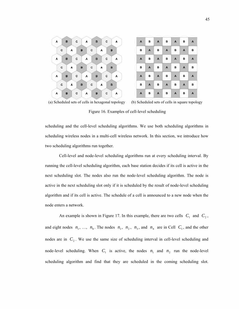
45

scheduling and the cell-level scheduling algorithms. We use both scheduling algorithms in

scheduling wireless nodes in a multi-cell wireless network. In this section, we introduce how

two scheduling algorithms run together.

Cell-level and node-level scheduling algorithms run at every scheduling interval. By

running the cell-level scheduling algorithm, each base station decides if its cell is active in the

next scheduling slot. The nodes also run the node-level scheduling algorithm. The node is

active in the next scheduling slot only if it is scheduled by the result of node-level scheduling

algorithm and if its cell is active. The schedule of a cell is announced to a new node when the

node enters a network.

An example is shown in Figure 17. In this example, there are two cells 1C and 2C ,

and eight nodes 1n , …, 8n . The nodes 1n , 2n , 3n , and 4n are in Cell 1C , and the other

nodes are in 2C . We use the same size of scheduling interval in cell-level scheduling and

node-level scheduling. When 1C is active, the nodes 1n and 2n run the node-level

scheduling algorithm and find that they are scheduled in the coming scheduling slot.

A B A B A B A

B A B A B A B

A B A B A B A

B A B A B A B

A B A B A B A

B A B A B A B

A B A B A B A

(a) Scheduled sets of cells in hexagonal topology (b) Scheduled sets of cells in square topology

Figure 16. Examples of cell-level scheduling

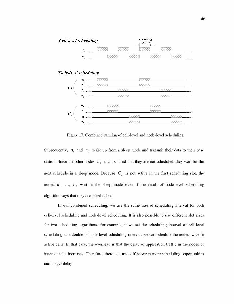
46

Subsequently, 1n and 2n wake up from a sleep mode and transmit their data to their base

station. Since the other nodes 3n and 4n find that they are not scheduled, they wait for the

next schedule in a sleep mode. Because 2C is not active in the first scheduling slot, the

nodes 5n , …, 8n wait in the sleep mode even if the result of node-level scheduling

algorithm says that they are schedulable.

In our combined scheduling, we use the same size of scheduling interval for both

cell-level scheduling and node-level scheduling. It is also possible to use different slot sizes

for two scheduling algorithms. For example, if we set the scheduling interval of cell-level

scheduling as a double of node-level scheduling interval, we can schedule the nodes twice in

active cells. In that case, the overhead is that the delay of application traffic in the nodes of

inactive cells increases. Therefore, there is a tradeoff between more scheduling opportunities

and longer delay.

Figure 17. Combined running of cell-level and node-level scheduling

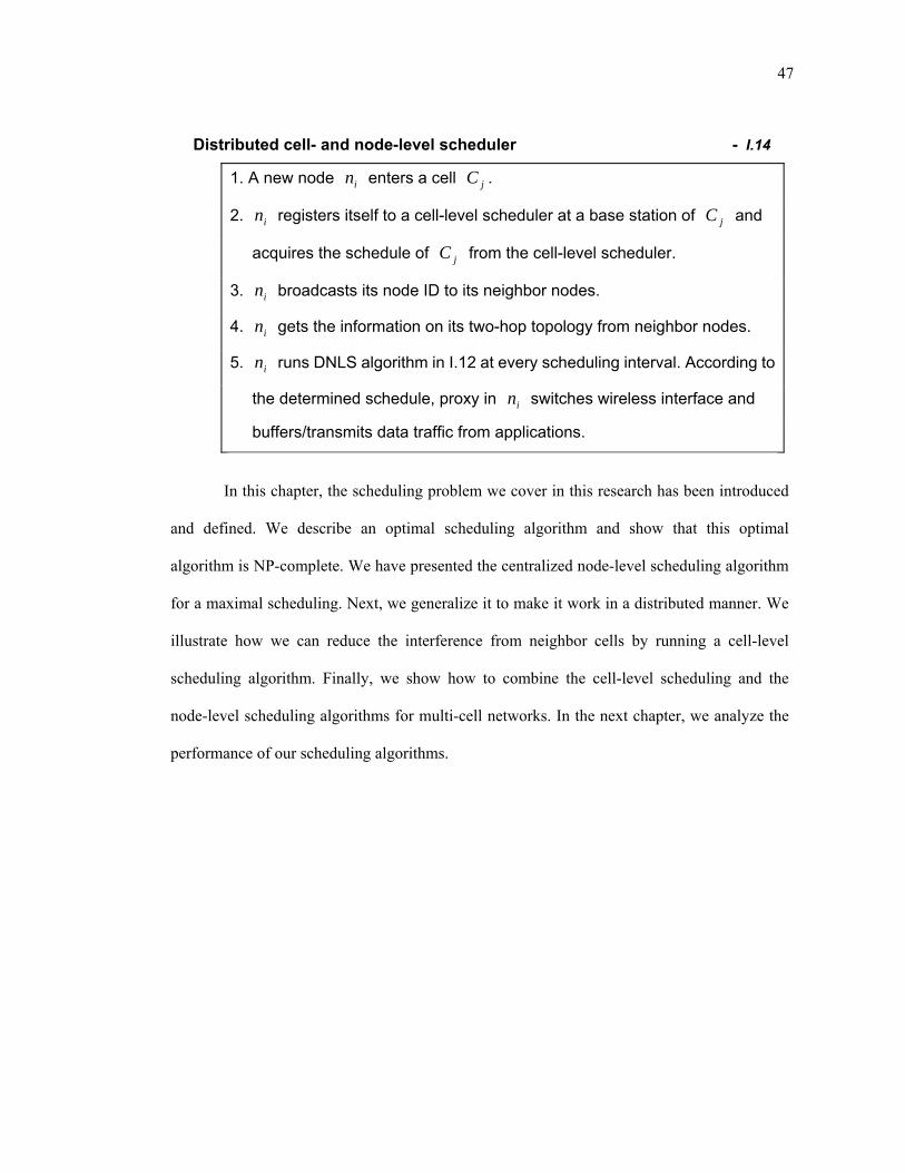
47

In this chapter, the scheduling problem we cover in this research has been introduced

and defined. We describe an optimal scheduling algorithm and show that this optimal

algorithm is NP-complete. We have presented the centralized node-level scheduling algorithm

for a maximal scheduling. Next, we generalize it to make it work in a distributed manner. We

illustrate how we can reduce the interference from neighbor cells by running a cell-level

scheduling algorithm. Finally, we show how to combine the cell-level scheduling and the

node-level scheduling algorithms for multi-cell networks. In the next chapter, we analyze the

performance of our scheduling algorithms.

Distributed cell- and node-level scheduler - I.14

1. A new node in enters a cell jC .

2. in registers itself to a cell-level scheduler at a base station of jC and

acquires the schedule of jC from the cell-level scheduler.

3. in broadcasts its node ID to its neighbor nodes.

4. in gets the information on its two-hop topology from neighbor nodes.

5. in runs DNLS algorithm in I.12 at every scheduling interval. According to

the determined schedule, proxy in in switches wireless interface and

buffers/transmits data traffic from applications.

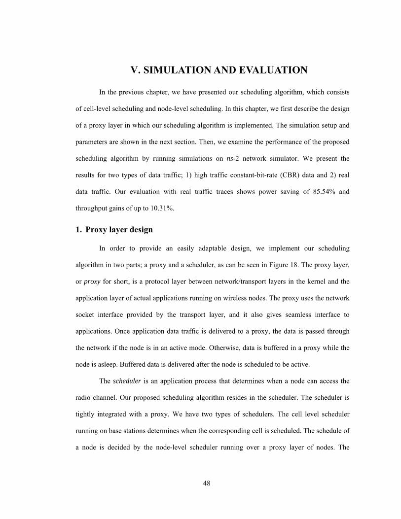
48

V. SIMULATION AND EVALUATION

In the previous chapter, we have presented our scheduling algorithm, which consists

of cell-level scheduling and node-level scheduling. In this chapter, we first describe the design

of a proxy layer in which our scheduling algorithm is implemented. The simulation setup and

parameters are shown in the next section. Then, we examine the performance of the proposed

scheduling algorithm by running simulations on ns-2 network simulator. We present the

results for two types of data traffic; 1) high traffic constant-bit-rate (CBR) data and 2) real

data traffic. Our evaluation with real traffic traces shows power saving of 85.54% and

throughput gains of up to 10.31%.

1. Proxy layer design

In order to provide an easily adaptable design, we implement our scheduling

algorithm in two parts; a proxy and a scheduler, as can be seen in Figure 18. The proxy layer,

or proxy for short, is a protocol layer between network/transport layers in the kernel and the

application layer of actual applications running on wireless nodes. The proxy uses the network

socket interface provided by the transport layer, and it also gives seamless interface to

applications. Once application data traffic is delivered to a proxy, the data is passed through

the network if the node is in an active mode. Otherwise, data is buffered in a proxy while the

node is asleep. Buffered data is delivered after the node is scheduled to be active.

The scheduler is an application process that determines when a node can access the

radio channel. Our proposed scheduling algorithm resides in the scheduler. The scheduler is

tightly integrated with a proxy. We have two types of schedulers. The cell level scheduler

running on base stations determines when the corresponding cell is scheduled. The schedule of

a node is decided by the node-level scheduler running over a proxy layer of nodes. The

48

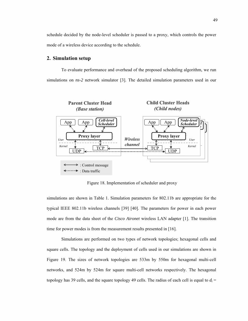
49

schedule decided by the node-level scheduler is passed to a proxy, which controls the power

mode of a wireless device according to the schedule.

2. Simulation setup

To evaluate performance and overhead of the proposed scheduling algorithm, we run

simulations on ns-2 network simulator [3]. The detailed simulation parameters used in our

simulations are shown in Table 1. Simulation parameters for 802.11b are appropriate for the

typical IEEE 802.11b wireless channels [39] [40]. The parameters for power in each power

mode are from the data sheet of the Cisco Aironet wireless LAN adapter [1]. The transition

time for power modes is from the measurement results presented in [16].

Simulations are performed on two types of network topologies; hexagonal cells and

square cells. The topology and the deployment of cells used in our simulations are shown in

Figure 19. The sizes of network topologies are 533m by 550m for hexagonal multi-cell

networks, and 524m by 524m for square multi-cell networks respectively. The hexagonal

topology has 39 cells, and the square topology 49 cells. The radius of each cell is equal to dt =

Wirelesschannel

: Control message: Data traffic

Parent Cluster Head(Base station)

Child Cluster Heads(Child nodes)

Proxy layerProxy layer

UDP

Cell-levelScheduler

TCP

App App

User

KernelProxy layerProxy layer

UDPTCP

App App

User

Kernel

Node-levelScheduler

Proxy layerProxy layer

UDPTCP

App App

User

Kernel

Node-levelScheduler

Proxy layerProxy layer

UDPTCP

App App

User

Kernel

Node-levelScheduler

Wirelesschannel

: Control message: Data traffic: Control message: Data traffic

Parent Cluster Head(Base station)

Child Cluster Heads(Child nodes)

Proxy layerProxy layer

UDP

Cell-levelScheduler

TCP

App App

User

Kernel

Proxy layerProxy layer

UDP

Cell-levelScheduler

TCP

App App

User

KernelProxy layerProxy layer

UDPTCP

App App

User

Kernel

Node-levelScheduler

Proxy layerProxy layer

UDPTCP

App App

User

Kernel

Node-levelScheduler

Proxy layerProxy layer

UDPTCP

App App

User

Kernel

Node-levelScheduler

Proxy layerProxy layer

UDPTCP

App App

User

Kernel

Node-levelScheduler

Proxy layerProxy layer

UDPTCP

App App

User

Kernel

Node-levelScheduler

Proxy layerProxy layer

UDPTCP

App App

User

Kernel

Node-levelScheduler

Figure 18. Implementation of scheduler and proxy

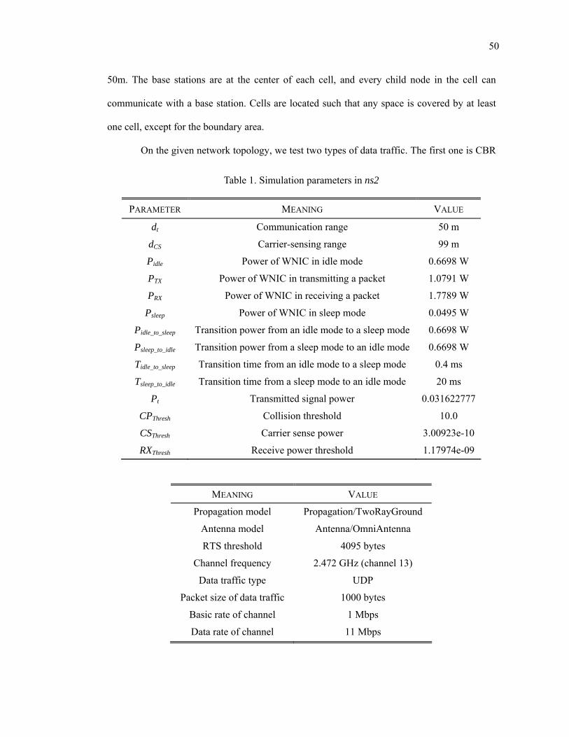
50

50m. The base stations are at the center of each cell, and every child node in the cell can

communicate with a base station. Cells are located such that any space is covered by at least

one cell, except for the boundary area.

On the given network topology, we test two types of data traffic. The first one is CBR

Table 1. Simulation parameters in ns2

PARAMETER MEANING VALUE

dt Communication range 50 m

dCS Carrier-sensing range 99 m

Pidle Power of WNIC in idle mode 0.6698 W

PTX Power of WNIC in transmitting a packet 1.0791 W

PRX Power of WNIC in receiving a packet 1.7789 W

Psleep Power of WNIC in sleep mode 0.0495 W

Pidle_to_sleep Transition power from an idle mode to a sleep mode 0.6698 W

Psleep_to_idle Transition power from a sleep mode to an idle mode 0.6698 W

Tidle_to_sleep Transition time from an idle mode to a sleep mode 0.4 ms

Tsleep_to_idle Transition time from a sleep mode to an idle mode 20 ms

Pt Transmitted signal power 0.031622777

CPThresh Collision threshold 10.0

CSThresh Carrier sense power 3.00923e-10

RXThresh Receive power threshold 1.17974e-09

MEANING VALUE

Propagation model Propagation/TwoRayGround

Antenna model Antenna/OmniAntenna

RTS threshold 4095 bytes

Channel frequency 2.472 GHz (channel 13)

Data traffic type UDP

Packet size of data traffic 1000 bytes

Basic rate of channel 1 Mbps

Data rate of channel 11 Mbps

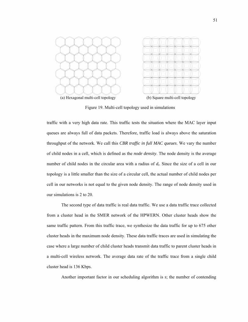
51

traffic with a very high data rate. This traffic tests the situation where the MAC layer input

queues are always full of data packets. Therefore, traffic load is always above the saturation

throughput of the network. We call this CBR traffic in full MAC queues. We vary the number

of child nodes in a cell, which is defined as the node density. The node density is the average

number of child nodes in the circular area with a radius of dt. Since the size of a cell in our

topology is a little smaller than the size of a circular cell, the actual number of child nodes per

cell in our networks is not equal to the given node density. The range of node density used in

our simulations is 2 to 20.

The second type of data traffic is real data traffic. We use a data traffic trace collected

from a cluster head in the SMER network of the HPWERN. Other cluster heads show the

same traffic pattern. From this traffic trace, we synthesize the data traffic for up to 675 other

cluster heads in the maximum node density. These data traffic traces are used in simulating the

case where a large number of child cluster heads transmit data traffic to parent cluster heads in

a multi-cell wireless network. The average data rate of the traffic trace from a single child

cluster head is 136 Kbps.

Another important factor in our scheduling algorithm is s; the number of contending

AP AP AP AP AP AP AP

AP AP AP AP AP AP AP

AP AP AP AP AP AP AP

AP AP AP AP AP AP AP

AP AP AP AP AP AP AP

AP AP AP AP AP AP AP

AP AP AP AP AP AP AP

(a) Hexagonal multi-cell topology (b) Square multi-cell topology

Figure 19. Multi-cell topology used in simulations

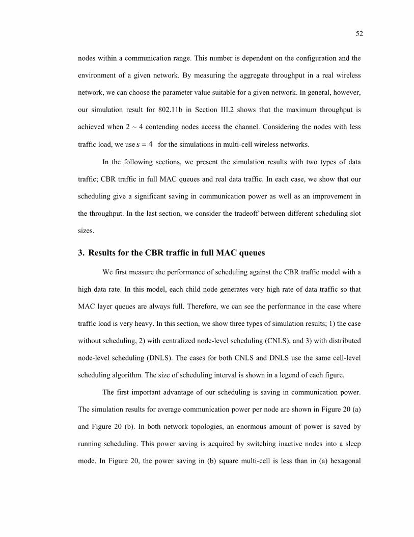
52

nodes within a communication range. This number is dependent on the configuration and the

environment of a given network. By measuring the aggregate throughput in a real wireless

network, we can choose the parameter value suitable for a given network. In general, however,

our simulation result for 802.11b in Section III.2 shows that the maximum throughput is

achieved when 2 ~ 4 contending nodes access the channel. Considering the nodes with less

traffic load, we use 4=s for the simulations in multi-cell wireless networks.

In the following sections, we present the simulation results with two types of data

traffic; CBR traffic in full MAC queues and real data traffic. In each case, we show that our

scheduling give a significant saving in communication power as well as an improvement in

the throughput. In the last section, we consider the tradeoff between different scheduling slot

sizes.

3. Results for the CBR traffic in full MAC queues

We first measure the performance of scheduling against the CBR traffic model with a

high data rate. In this model, each child node generates very high rate of data traffic so that

MAC layer queues are always full. Therefore, we can see the performance in the case where

traffic load is very heavy. In this section, we show three types of simulation results; 1) the case

without scheduling, 2) with centralized node-level scheduling (CNLS), and 3) with distributed

node-level scheduling (DNLS). The cases for both CNLS and DNLS use the same cell-level

scheduling algorithm. The size of scheduling interval is shown in a legend of each figure.

The first important advantage of our scheduling is saving in communication power.

The simulation results for average communication power per node are shown in Figure 20 (a)

and Figure 20 (b). In both network topologies, an enormous amount of power is saved by

running scheduling. This power saving is acquired by switching inactive nodes into a sleep

mode. In Figure 20, the power saving in (b) square multi-cell is less than in (a) hexagonal

53

multi-cell. This is because cells in square multi-cell topology are scheduled more often, every

two time slots. As the node density increases, we get higher power saving. When the node

density is high, a node has a lower chance of being scheduled. Accordingly, we get more

power savings. Maximum power savings reach up to 80%.

The next point to consider is throughput. The throughput is measured at the base

0.0

0.2

0.4

0.6

0.8

1.0

1.2

0 4 8 12 16 20

Node density

Pow

er (W

) No schedulingCNLS (0.3sec)DNLS (0.3sec)

0.0

0.2

0.4

0.6

0.8

1.0

1.2

0 4 8 12 16 20

Node density

Pow

er (W

)

(a) Power in hexagonal multi-cell (b) Power in square multi-cell

1.0

1.2

1.4

1.6

1.8

0 4 8 12 16 20

Node density

Thro

ughp

ut p

er c

ell (

Mbp

s)

No schedulingCNLS (0.3sec)DNLS (0.3sec)

1.0

1.2

1.4

1.6

1.8

0 4 8 12 16 20

Node density

Thro

ughp

ut p

er c

ell (

Mbp

s)

(c) Throughput in hexagonal multi-cell (d) Throughput in square multi-cell

0.00

0.01

0.02

0.03

0.04

0.05

0.06

0.07

0 4 8 12 16 20Node density

Del

ay (s

ec)

No schedulingCNLS (0.3sec)DNLS (0.3sec)

0.00

0.01

0.02

0.03

0.04

0.05

0.06

0.07

0 4 8 12 16 20Node density

Del

ay (s

ec)

(e) Transmission delay in hexagonal multi-cell (f) Transmission delay in square multi-cell

Figure 20.Results for the CBR traffic model

54

stations. Figure 20 (c) and (d) show the measured average throughput for the CBR traffic in

full MAC queues. In Figure 20 (c), we find that scheduling improves the average throughput

significantly. This improvement is due to the reduction of contention in the radio channel. To

understand how much time is spent in transmitting a packet on the MAC layer, we measured

the transmission delay of a data packet. Transmission delay is defined as the delay from the

receipt of a data packet at MAC layer until a data packet is acknowledged by an ACK packet

in the MAC layer, coming from a receiver node. The measured result is shown in Figure 20 (e)

and (f). In both topologies, transmission delay increases gradually as the network density goes

up. By running our scheduling algorithm, we can control the transmission delay at the same

level as the delay for a network with the node density of 4. Thus, we can say that the amount

of contention by running our scheduling is very close to the case when only four nodes

contend for accessing the channel within a communication range.

We also find that two scheduling algorithms, centralized node-level scheduling

(CNLS) algorithm and distributed node-level scheduling (DNLS) algorithm, give very similar

results in communication power and throughput. This is because two algorithms schedule

almost the same number of child nodes in an active cell. This means that the performance of

DNLS algorithm is very close to that of CNLS algorithm. In terms of the number of scheduled

active nodes, DNLS algorithm gives the result very close to that of CNLS algorithm. If the

number of active nodes is too small, we get lower average throughput because the active

nodes cannot fully exploit available channel bandwidth. If the number of nodes scheduled by

DNLS algorithm is too large, we cannot reduce the contention in a channel enough. Thus, we

get the lower throughput. In the other performance metrics such as power and delay, we

observe the same results. Therefore, from the next section, we only present the results for the

DNLS algorithm.

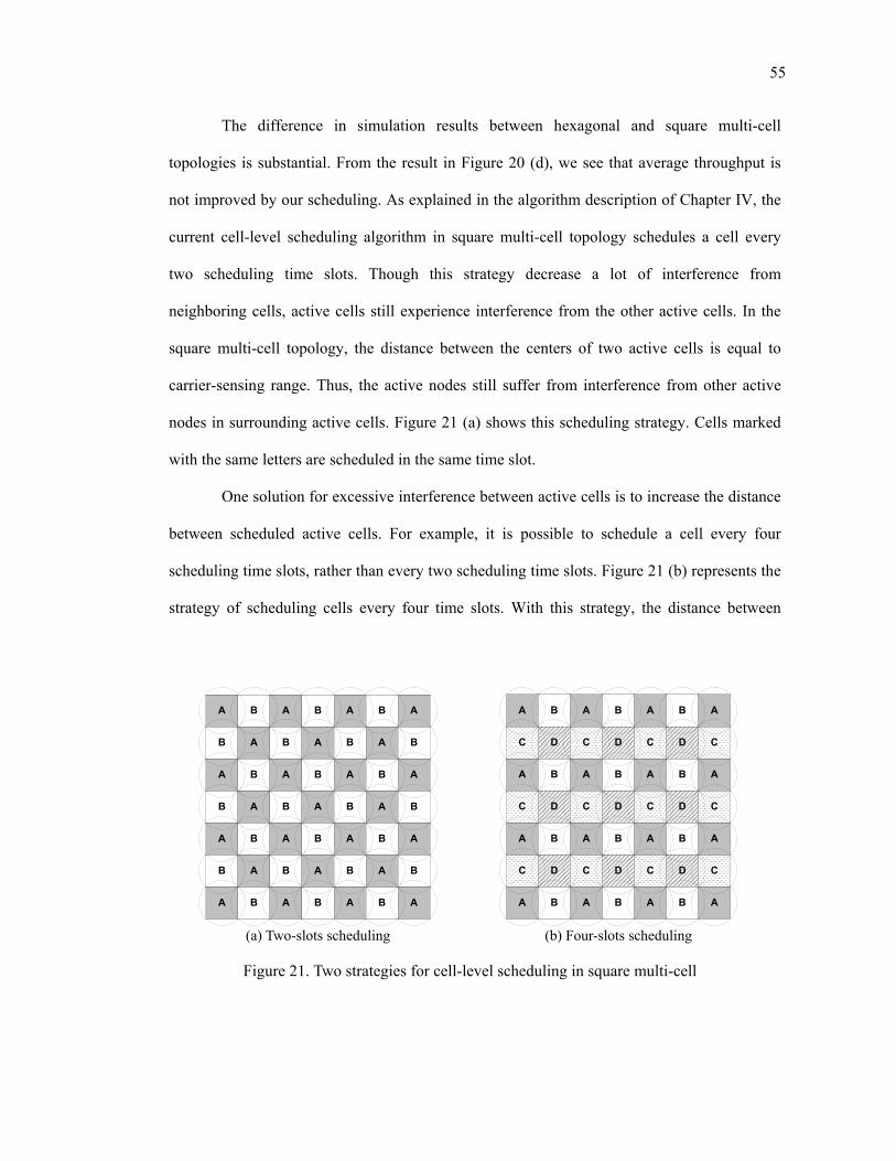
55

The difference in simulation results between hexagonal and square multi-cell

topologies is substantial. From the result in Figure 20 (d), we see that average throughput is

not improved by our scheduling. As explained in the algorithm description of Chapter IV, the

current cell-level scheduling algorithm in square multi-cell topology schedules a cell every

two scheduling time slots. Though this strategy decrease a lot of interference from

neighboring cells, active cells still experience interference from the other active cells. In the

square multi-cell topology, the distance between the centers of two active cells is equal to

carrier-sensing range. Thus, the active nodes still suffer from interference from other active

nodes in surrounding active cells. Figure 21 (a) shows this scheduling strategy. Cells marked

with the same letters are scheduled in the same time slot.

One solution for excessive interference between active cells is to increase the distance

between scheduled active cells. For example, it is possible to schedule a cell every four

scheduling time slots, rather than every two scheduling time slots. Figure 21 (b) represents the

strategy of scheduling cells every four time slots. With this strategy, the distance between

A B A B A B A

B A B A B A B

A B A B A B A

B A B A B A B

A B A B A B A

B A B A B A B

A B A B A B A

A B A B A B A

C D C D C D C

A B A B A B A

C D C D C D C

A B A B A B A

C D C D C D C

A B A B A B A

(a) Two-slots scheduling (b) Four-slots scheduling

Figure 21. Two strategies for cell-level scheduling in square multi-cell

56

active cells is far enough to completely remove interference among active cells. But, this

scheme reveals a critical disadvantage in improving throughput. Because the number of active

cells for a time slot is smaller in four-slots scheduling of Figure 21 (b) than in two-slots

scheduling of Figure 21 (a), it is very difficult for a four-slot scheduling to achieve any

improvement in throughput. Therefore, the average throughput by four-slots scheduling of

Figure 21 (b) is less than in the case without any scheduling at all. In other words, we can say

that active cell’s spatial parallelism in a network topology is an important factor in

determining the throughput improvement achievable by scheduling. In a hexagonal multi-cell

topology, locations of active cells maximize scheduling throughput gain because the active

cells are far enough to eliminate most of interference between active cells while they are close

enough to exploit spatial parallelism in a given field area. Therefore, by running the

scheduling over an appropriate network topology, we can get more benefits than just reduced

power, e.g., throughput gain.

4. Results for the real data traffic

We next take a look at the simulation results from real data traffic. The CBR traffic

model in the previous section is to measure the performance under the heavy traffic loads. In

this section, the simulation with real data traffic shows how our scheduling performs in the

case where a network contains a large number of the child cluster heads. The results on

communication power, average throughput per cell, and MAC layer transmission delay are

presented. In addition, we discuss the application layer delay in detail.

We first observe great power savings when running scheduling in both hexagonal and

square multi-cell topology. In Figure 22 (a) and (b), DNLS-based scheduling saves up to

85.54 % of communication power in the hexagonal multi-cell case and up to 78.63 % in the

square multi-cell case. The higher power savings in hexagonal case are due to the longer sleep

57

period from the cell-level scheduling. The observed values of communication power for the

case with no scheduling show a different pattern from the values in Figure 20. In Figure 20 (a)

and (b), we see that communication power is almost flat. However, in Figure 22 (a) and (b),

the power increases gradually until it becomes saturated. At the full MAC-layer queue model

in Figure 20, the network channel is always congested by traffic since MAC layer queues in

nodes are always full. But the nodes of the real traffic model in Figure 22 have an average data

rate of 136 Kbps. Until the network channel is fully congested by traffic, wireless devices

work in an idle mode for the large amount of time. While it is in an idle mode, wireless

devices consume less power. Therefore, the communication power in the real-traffic model is

less than the power in high data rate CBR model until the network channel is saturated by data

traffic. In both of Figure 20 and Figure 22, our scheduling achieves significant power savings.

Average throughput and MAC layer transmission delay are shown from Figure 22 (c)

to (f). In a hexagonal multi-cell topology, we see that our scheduling improves the average

throughput when traffic load is above the saturation level of the network, which is 1.1 Mbps

without scheduling. The throughput gained by scheduling is up to 10.31 %. In the square

multi-cell topology, however, we find a different result. In this case, running our scheduling

only decreases the throughput up to 7.27 %. As pointed out in the previous section and in

Figure 20, this is caused by the distribution of active cells in square multi-cell topology that is

too dense to eliminate interference from other active cells. In a square multi-cell, the distance

between active cells is not far enough to remove most of inter-cell interference. Therefore

each active cell cannot obtain the maximum throughput.

58

We next discuss the application layer delay. Application layer delay is the time delay

that applications running on wireless nodes experience. This is the actual delay in delivering a

fixed-size data packet from a sender application to a receiver application. Using our

0.0

0.2

0.4

0.6

0.8

1.0

1.2

0.0 0.5 1.0 1.5 2.0 2.5

Traffic load (Mbps)

Pow

er (W

)

No scheduling

DNLS (0.3sec)

0.0

0.2

0.4

0.6

0.8

1.0

1.2

0.0 0.5 1.0 1.5 2.0

Traffic load (Mbps)

Pow

er (W

)

c

(a) Power in hexagonal multi-cell (b) Power in square multi-cell

0.0

0.2

0.4

0.6

0.8

1.0

1.2

1.4

0.0 0.5 1.0 1.5 2.0 2.5Traffic load (Mbps)

Thro

ughp

ut p

er c

ell (

Mbp

s)

No scheduling

DNLS (0.3sec)

0.0

0.2

0.4

0.6

0.8

1.0

1.2

0.0 0.5 1.0 1.5 2.0Traffic load (Mbps)

Thro

ughp

ut p

er c

ell (

Mbp

s)

(c) Throughput in hexagonal multi-cell (d) Throughput in square multi-cell

0.000

0.005

0.010

0.015

0.020

0.025

0.030

0.0 0.5 1.0 1.5 2.0 2.5

Traffic load (Mbps)

Del

ay (s

ec)

No scheduling

DNLS (0.3sec)

0.000

0.005

0.010

0.015

0.020

0.025

0.030

0.0 0.5 1.0 1.5 2.0

Traffic load (Mbps)

Del

ay (s

ec)

(e) Transmission delay in hexagonal multi-cell (f) Transmission delay in square multi-cell

Figure 22. Results for the real traffic data model

59

scheduling algorithm on a given network reduces the number of contending nodes in a channel.

Consequently, the MAC layer delay is reduced. However, because of the scheduling interval

based scheme of our scheduling algorithm, it is inevitable that the actual application layer

delay increases accordingly. The results on application layer delay for the real-traffic model

are shown in Figure 23. We limit the maximum value of the horizontal axis, the amount of

traffic load, to 1.4 Mbps. Once the traffic load exceeds the maximum throughput experienced

by the case with no scheduling (which is 1.1 Mbps in Figure 22 (a) and (b)), application layer

delay increases dramatically.

For the cases of Figure 23 where scheduling is applied, applications experience a

certain level of application layer delay; in the case of the scheduling slot size of 0.3 second,

delay is at least 0.4 second in the hexagonal and 0.26 seconds in the square multi-cell. This

delay is due to the unscheduled nodes that wait in a sleep mode while buffering data from

applications. We also see a difference in the minimum amount of delay between the two

topologies. The square multi-cell topology experiences a lower value in the minimum delay.

This is because the cell-level scheduling algorithm uses two time slots for scheduling all cells,

0.0

1.0

2.0

3.0

4.0

0.0 0.2 0.4 0.6 0.8 1.0 1.2 1.4

Traffic load (Mbps)

Del

ay (s

ec)

No schedulingDNLS (0.1sec)DNLS (0.3sec)DNLS (0.5sec)

0.0

1.0

2.0

3.0

4.0

0.0 0.2 0.4 0.6 0.8 1.0 1.2 1.4

Traffic load (Mbps)

Del

ay (s

ec)

(a) Delay in hexagonal multi-cell (b) Delay in square multi-cell

Figure 23. Application layer delay in a real-traffic model

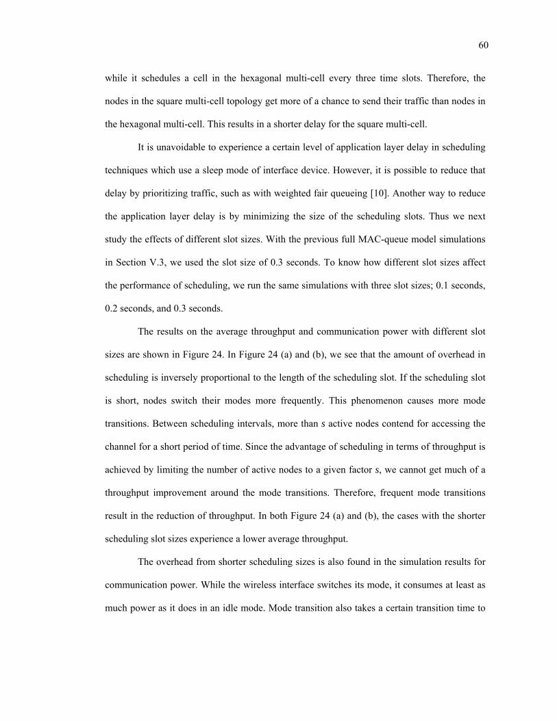
60

while it schedules a cell in the hexagonal multi-cell every three time slots. Therefore, the

nodes in the square multi-cell topology get more of a chance to send their traffic than nodes in

the hexagonal multi-cell. This results in a shorter delay for the square multi-cell.

It is unavoidable to experience a certain level of application layer delay in scheduling

techniques which use a sleep mode of interface device. However, it is possible to reduce that

delay by prioritizing traffic, such as with weighted fair queueing [10]. Another way to reduce

the application layer delay is by minimizing the size of the scheduling slots. Thus we next

study the effects of different slot sizes. With the previous full MAC-queue model simulations

in Section V.3, we used the slot size of 0.3 seconds. To know how different slot sizes affect

the performance of scheduling, we run the same simulations with three slot sizes; 0.1 seconds,

0.2 seconds, and 0.3 seconds.

The results on the average throughput and communication power with different slot

sizes are shown in Figure 24. In Figure 24 (a) and (b), we see that the amount of overhead in

scheduling is inversely proportional to the length of the scheduling slot. If the scheduling slot

is short, nodes switch their modes more frequently. This phenomenon causes more mode

transitions. Between scheduling intervals, more than s active nodes contend for accessing the

channel for a short period of time. Since the advantage of scheduling in terms of throughput is

achieved by limiting the number of active nodes to a given factor s, we cannot get much of a

throughput improvement around the mode transitions. Therefore, frequent mode transitions

result in the reduction of throughput. In both Figure 24 (a) and (b), the cases with the shorter

scheduling slot sizes experience a lower average throughput.

The overhead from shorter scheduling sizes is also found in the simulation results for

communication power. While the wireless interface switches its mode, it consumes at least as

much power as it does in an idle mode. Mode transition also takes a certain transition time to

61

wake up and to go sleep. Specific parameters are in Table 1 in the previous chapter. Thus, it is

expected that scheduling with the shorter slot size reveals more overhead in energy

consumption. The results in Figure 24 (c) and (d) show that the overhead in power increases as

the slot size decreases.

From the perspective of throughput and power, we can say that it is better to use a

longer stretch for the scheduling time slot. The use of a longer scheduling slot improves the

average throughput and saves more communication power, but causes a longer delay. The

tradeoff between the improvements in throughput and power and the cost in terms of delay is a

key issue in determining the scheduling slot size.

1.0

1.2

1.4

1.6

1.8

0 4 8 12 16 20

Node density

Thro

ughp

ut p

er c

ell (

Mbp

s)

No schedulingDNLS (0.1sec)DNLS (0.2sec)DNLS (0.3sec)

1.0

1.2

1.4

1.6

1.8

0 4 8 12 16 20

Node density

Thro

ughp

ut p

er c

ell (

Mbp

s)

(a) Throughput in hexagonal multi-cell (b) Throughput in square multi-cell

0.0

0.2

0.4

0.6

0.8

1.0

1.2

0 4 8 12 16 20

Node density

Pow

er (W

)

No schedulingDNLS (0.1sec)DNLS (0.2sec)DNLS (0.3sec)

0.0

0.2

0.4

0.6

0.8

1.0

1.2

0 4 8 12 16 20

Node density

Pow

er (W

)

(c) Power in hexagonal multi-cell (d) Power in square multi-cell

Figure 24. Throughput and power for different slot sizes

62

In this chapter, we have evaluated our scheduling algorithms by running simulations

with two types of data traffic patterns. We achieve large amount of communication power

savings: up to 80.38% for CBR traffic and up to 85.45% for real data traffic. The maximum

throughput gains are 9.48% and 10.24% respectively.

63

VI. CONCLUSIONS

In this thesis, we have presented a hybrid distributed multi-cell scheduling algorithm.

We have shown that a falloff in an aggregate throughput in a large-scale multi-cell wireless

network is due to both interference between neighboring cells and the contention among nodes.

To remove interference between cells, we presented a distributed cell-level scheduling

algorithm. To solve the problem of contention among nodes, we proposed an optimal

node-level scheduling algorithm for a maximum scheduling. Moreover, we proved that the

algorithm for a maximum scheduling is NP-complete for any 1≥s . Because running an

NP-complete algorithm at runtime is not practical in large-scale multi-cell wireless networks,

we proposed the centralized node-level scheduling algorithm that is a solution for the simpler

maximal scheduling problem. Next, we converted this algorithm into a distributed node-level

scheduling algorithm. Finally, we combined the cell-level scheduling and the node-level

scheduling algorithms to run our scheduling in a wireless network consisting of large number

of cells.

Our proposed scheduling algorithms run on a proxy layer. Proxy is a virtualization

mechanism that provides a seamless application interface while minimizing modification of

existing network protocol implementation in the kernel. By running the scheduling algorithms

on the proxy layer, we are able to show that a novel scheduling algorithm can run over the

existing network and MAC layers, using off-the-shelf network components.

The proposed scheduling algorithm runs on multi-cell heterogeneous wireless

networks. Our scheduling mechanism provides the control of channel access and throughput

allocation to the sensor node cluster heads. We can get an improvement in aggregate

throughput by reducing both the contention between the nodes and the interference between

63

64

the neighboring cells. Saving communication power while achieving an increase in throughput

is a big accomplishment of our proposed algorithm.

To evaluate the performance of the proposed scheduling algorithm in a real network,

we have run the simulations with the real traces of data traffic collected at the cluster head

nodes in the SMER network. In those experiments, we see an improvement in average

throughput of up to 10.31 % in hexagonal multi-cell networks, with maximum power saving

of 85.54 %.

We also measured the overhead of scheduling on delay in data delivery. By measuring

the application layer delay of delivered data traffic, we concluded that the size of scheduling

time slot determines the minimum possible delay. Different scheduling slot sizes affect the

overhead in throughput, power saving, and delay. Therefore, it is important to find the right

tradeoff between the benefits of scheduling and the cost in delay. With the current randomized

scheduling algorithm we recommend choosing a longer scheduling slot size if the delay

requirements of applications are satisfied. In addition, the application layer delay can be

further optimized by introducing traffic priorities. We leave this for future work.

65

VII. REFERENCES

[1] Cisco Aironet 802.11a/b/g CardBus wireless LAN adapter data sheet, http://www.cisco.com/en/US/products/hw/wireless/ps4555/products_data_sheet09186a00801ebc29.html, Cisco Systems.

[2] High Performance Wireless Research and Education Network (HPWREN), http://hpwren.ucsd.edu/

[3] ns-2 network simulator, http://www.isi.edu/nsnam/ns/ [4] G. Ahn, A. T. Campbell, A. Veres, and L. Sun, “SWAN: Service differentiation in

stateless wireless ad hoc networks,” in IEEE INFOCOM, 2002. [5] E. Arikan, “Multi-access in packet-radio networks,” M.Sc. thesis, MIT, LIDS-TH-1234,

1982. [6] M. Bottigliengo, C. Casetti, C. Chiasserini, and M. Meo, “Smart traffic scheduling in

802.11 WLANs with access point,” IEEE Vehicular Technology Conference, 2003. [7] R. Bruno, M. Conti, and E. Gregori, “Mesh networks: commodity multihop ad hoc

networks,” IEEE Communications Magazine, 2005. [8] S. Choi, K. Park, and C. Kim, “On the performance characteristics of WLANs: revisited,”

ACM SIGMETRICS, 2005. [9] I. Cidon, and M. Sidi, “Distributed assignment algorithms for multihop packet radio

networks,” IEEE Transactions on Computers, 1989. [10] A. Demers, “Analysis and simulation of a fair queueing algorithm,” ACM SIGCOMM,

1989. [11] T. Elbatt and A. Ephremides, “Joint scheduling and power control for wireless ad hoc

networks,” IEEE Transactions on Wireless Communications, 2004. [12] V. Gambiroza, B. Sadeghi, and E. W. Knightly, “End-to-end performance and fairness

in multihop wireless backhaul networks,” MOBICOM, 2004. [13] W. K. Hale, “Frequency assignment: theory and applications,” Proc. IEEE, 1980. [14] M. Heusse, F. Rousseau, G. Berger-Sabbatel, and A. Duda, “Performance anomaly of

802.11b,” IEEE INFOCOM, 2003. [15] B. Hohlt, L. Doherty, and E. Brewer, “Flexible power scheduling for sensor networks,”

International Symposium on Information Processing in Sensor Networks (IPSN), 2004. [16] K. Jamieson, “Implementation of a power-saving protocol for ad hoc wireless networks”,

Master's thesis, Massachusetts Institute of Technology, Feb. 2002. [17] J. Jun, P. Peddabachagari, M. Sichitiu, “Theoretical maximum throughput of IEEE

802.11 and its applications,” IEEE International Symposium on Network Computing and Applications, 2003.

[18] E. Jung and N. H. Vaidya, “An energy efficient MAC protocol for wireless LANs,” in IEEE INFOCOM, 2002.

65

66

[19] R. Karrer, A. Sabharwal, and E. Knightly, “Enabling large-scale wireless broadband: the case for TAPs,” ACM SIGCOMM Computer Communications Review, 2004.

[20] L. Kleinrock and F. Tobagi, “Packet Switching in Radio Channels Part II - the Hidden Node Problem in Carrier Sense Multiple Access Nodes and the Busy Tone Solution,” in IEEE Transactions on Communications, vol. COM-23, no. 12, pp. 1417-1433, 1975.

[21] D. Lim, J. Shim, T. S. Rosing, and T. Javidi, “Scheduling data delivery in heterogeneous wireless sensor networks,” in IEEE International Symposium on Multimedia (ISM 2006), Dec. 2006.

[22] S. Mangold, S. Choi, P. May, O. Klein, G. Hiertz, and L. Stibor, “IEEE 802.11e wireless LAN for quality of service,” European Wireless, 2002.

[23] V. Mhatre and C. Rosenberg, “Homogeneous vs heterogeneous clustered sensor networks: a comparative study,” IEEE International Conference on Communications, 2004.

[24] M. Petrovic and M. Aboelaze, “Performance of TCP/UDP under ad hoc IEEE 802.11,” International Conference on Telecommunications, 2003.

[25] L. Pond and V. Li, “A distributed time-slot assignment protocol for mobile multi-hop broadcast packet radio networks,” IEEE MILCOM, 1989.

[26] W. Qadeer, T. Simunic, J. Ankcorn, V. Krishnan, and G. D. Micheli, “Heterogeneous wireless network management,” Power-Aware Computer Systems, 2003.

[27] R. Ramaswami, and K. Parhi, “Distributed scheduling of broadcasts in a radio network,” IEEE INFOCOM, 1989.

[28] A. Rao and I. Stoica, “An overlay MAC layer for 802.11 networks,” ACM MOBICOM, 2005.

[29] P. A. Raymond, “Performance analysis of cellular networks,” IEEE Transactions of Communications, 1991.

[30] J. Rexford, S. Sen, and A. Basso, “A smoothing proxy service for variable-bit-rate streaming video,” in IEEE GLOBECOM, 1999.

[31] B. Sadeghi, V. Kanodia, A. Sabharwal, and E. Knightly, “Opportunistic media access for multirate ad hoc networks,” ACM MOBICOM, September, 2002, Atlanta, Georgia.

[32] P. Shenoy and P. Radkov, “Proxy-assisted power-friendly streaming to mobile devices,” Multimedia Computing and Networking, 2003.

[33] T. Simunic, W. Qadeer, and G. D. Micheli, “Managing heterogeneous wireless environments via Hotspot servers,” Multimedia Computing and Networking, 2005.

[34] J. Snow, W. Feng, and W. Feng, “Implementing a low power TDMA protocol over 802.11,” IEEE Wireless Communications and Networking Conference, 2005.

[35] N. H. Vaidya, P. Bahl, and S. Gupta, “Distributed fair scheduling in a wireless LAN”, ACM MOBICOM, 2000.

[36] A. Vasan and A.U. Shankar, “An empirical characterization of instantaneous throughput in 802.11b WLANs,” Technical report, Department of Computer Science, University of Maryland, 2002.

67

[37] S. Waharte, J. Xiao, and R. Boutaba, “Overlay wireless sensor networks for application-adaptive scheduling in WLAN,” IEEE Conference on High Speed Networks and Multimedia Communications, 2004.

[38] H. Wu, Q. Luo, and W. Xue, “Distributed cross-layer scheduling for in-network sensor query processing,” IEEE International Conference on Pervasive Computing and Communications (PERCOM), 2006.

[39] W. Xiuchao, “Simulate 802.11b channel within ns2”, Technical report, School of Computing, National University of Singapore , 2004.

[40] W. Xiuchao and A. L. Ananda, “Link characteristics estimation for IEEE 802.11 DCF based LAN,” IEEE Conference on Local Computer Networks, 2004.

[41] Y. Yi and S. Shakkottai, “Hop-by-hop congestion control over a wireless multi-hop network,” IEEE INFOCOM, 2004.

[42] F. Yu, Q. Zhang, W. Zhu, and Y. Zhang, “QoS-adaptive proxy caching for multimedia streaming over the internet,” in IEEE Transactions on Circuits and Systems for Video Technology, Vol. 13, No. 3, March 2003.

[43] J. Zander, “Performance of optimum transmitter power control in cellular radio systems,” IEEE Transactions on Vehicular Technology, 1992

[44] H. Zhai, J. Wang, and Y. Fang, “Distributed packet scheduling for multihop flows in ad hoc networks,” IEEE Wireless Communications and Networking Conference, 2004.