Distributed Programming over Time-series GraphsYogesh Simmhan, Neel Choudhury

Indian Institute of Science, Bangalore 560012 Indiasimmhan@serc.iisc.in, neel@ssl.serc.iisc.in

Charith Wickramaarachchi, Alok Kumbhare,Marc Frincu, Cauligi Raghavendra, Viktor Prasanna

Univ. of Southern California, Los Angeles CA 90089 USA{cwickram,kumbhare,frincu,raghu,prasanna}@usc.edu

Abstract—Graphs are a key form of Big Data, and performingscalable analytics over them is invaluable to many domains. Thereis an emerging class of inter-connected data which accumulatesor varies over time, and on which novel algorithms both overthe network structure and across the time-variant attributevalues is necessary. We formalize the notion of time-seriesgraphs and propose a Temporally Iterative BSP programmingabstraction to develop algorithms on such datasets using severaldesign patterns. Our abstractions leverage a sub-graph centricprogramming model and extend it to the temporal dimension.We present three time-series graph algorithms based on thesedesign patterns and abstractions, and analyze their performanceusing the GoFFish distributed platform on Amazon AWS Cloud.Our results demonstrate the efficacy of the abstractions todevelop practical time-series graph algorithms, and scale themon commodity hardware.

I. INTRODUCTION

There is a rapid proliferation of ubiquitous physical sensors,personal devices and virtual agents that sense, monitor andtrack human and environmental activity as part of the evolvingInternet of Things (IoT) [1]. Data streaming continuouslyor periodically from such domains are intrinsically intercon-nected and grow immensely in size. These often possess twokey characteristics: (1) temporal attributes and (2) networkrelationships that exist between them. Such datasets thatimbue both these temporal and graph features have not beenadequately examined in Big Data literature even as they arebecoming pervasive.

For example, consider a road network in a Smart City. Theroad topology remains relatively static over days. However,the traffic volume monitored on each road segment changessignificantly throughout the day [2], as do the actual vehi-cles that are captured by traffic cameras. Widespread urbanmonitoring systems, community mapping apps 1, and theadvent of self-driving cars will continue to enhance our abilityto rapidly capture changing road information for both real-time and offline analytics. There are many similar networkdatasets where the graph topology changes incrementally butattributes of vertices and edges vary often. These include SmartPower Grids (changing power flows on edges, power con-sumption at vertices), communication infrastructure (varyingedge bandwidths between endpoints) [3], and environmentalsensor networks (real-time observations from sensor vertices).Despite their seeming dynamism, even social network graphstructures change more slowly compared to the number of

1https://www.waze.com/

tweets or messages exchanged over the network 2. Analyticsthat range from intelligent traffic routing to epidemiologystudies on how diseases spread are possible on these.

Graph datasets with temporal characteristics have beenvariously known in literature as temporal graphs [4],kineographs [5], dynamic graphs [6] and time-evolvinggraphs [7]. Temporal graphs capture the time variant networkstructure in a single graph by introducing a temporal edgebetween the same vertex at different moments. Others con-struct graph snapshots at specific change points in the graphstructure, while Kineograph deal with graph that exhibit highstructural dynamism. As such, the exploration into such graphswith temporal features is at an early stage (§ V).

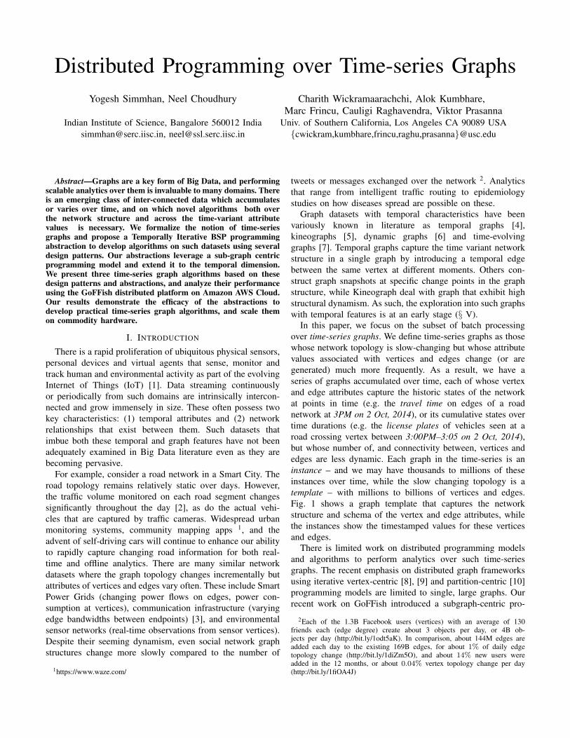
In this paper, we focus on the subset of batch processingover time-series graphs. We define time-series graphs as thosewhose network topology is slow-changing but whose attributevalues associated with vertices and edges change (or aregenerated) much more frequently. As a result, we have aseries of graphs accumulated over time, each of whose vertexand edge attributes capture the historic states of the networkat points in time (e.g. the travel time on edges of a roadnetwork at 3PM on 2 Oct, 2014), or its cumulative states overtime durations (e.g. the license plates of vehicles seen at aroad crossing vertex between 3:00PM–3:05 on 2 Oct, 2014),but whose number of, and connectivity between, vertices andedges are less dynamic. Each graph in the time-series is aninstance – and we may have thousands to millions of theseinstances over time, while the slow changing topology is atemplate – with millions to billions of vertices and edges.Fig. 1 shows a graph template that captures the networkstructure and schema of the vertex and edge attributes, whilethe instances show the timestamped values for these verticesand edges.

There is limited work on distributed programming modelsand algorithms to perform analytics over such time-seriesgraphs. The recent emphasis on distributed graph frameworksusing iterative vertex-centric [8], [9] and partition-centric [10]programming models are limited to single, large graphs. Ourrecent work on GoFFish introduced a subgraph-centric pro-

2Each of the 1.3B Facebook users (vertices) with an average of 130friends each (edge degree) create about 3 objects per day, or 4B ob-jects per day (http://bit.ly/1odt5aK). In comparison, about 144M edges areadded each day to the existing 169B edges, for about 1% of daily edgetopology change (http://bit.ly/1diZm5O), and about 14% new users wereadded in the 12 months, or about 0.04% vertex topology change per day(http://bit.ly/1fiOA4J)

Graph ID, 34567890Time, start, duration(Attribute Name, Value)*

Graph ID, Long(Attribute Name, Type)*

Vertex ID, Long(Attribute Name, Type)*

Edge ID, Long(Attribute Name, Type)*

Vertex ID, 12345678(Attribute Name, Value)*

Edge ID, 23456789(Attribute Name, Value)*

Graph Template

Graph Instances

time

Graph ID, 34567890Time, start, duration(Attribute Name, Value)*

Graph ID, Long(Attribute Name, Type)*

Vertex ID, Long(Attribute Name, Type)*

Edge ID, Long(Attribute Name, Type)*

Graph Template Graph Instances

time

…Vertex ID, 12345678(Attribute Name, Type)*

Edge ID, 23456789(Attribute Name, Type)*

Figure 1. Time-series graph collection. Template captures static topology andattribute names. Instances record temporally variant attribute values.

gramming model [11] and algorithms [12] over single, dis-tributed graphs that significantly out-performs vertex-centricmodels. In this paper, we focus on a programming model foranalysis over a collection of distributed time-series graphs, anddevelop graph algorithms that benefit from them. In particular,we target applications where the result of computation ona graph instance in one timestep is necessary to process agraph instance in the next timestep [13]. We refer to thisclass of algorithm as sequentially-dependent temporal graphalgorithms, or simply, sequentially-dependent algorithms.

We make the following specific contributions in this paper:1) We define a time-series graph data model, and propose

a Temporally Iterative Bulk Synchronous Parallel (TI-BSP) programming abstraction to support several designpatterns for temporal graph algorithms (§ II);

2) We develop three time-series graph algorithms that ben-efit from these abstractions: Time-Dependent ShortestPath, Meme Tracking, and Hashtag Aggregation (§ III);

3) We empirically evaluate and analyze these three algo-rithms on GoFFish, a distributed graph processing frame-work that implements the TI-BSP abstraction. (§ IV).II. PROGRAMMING OVER TIME-SERIES GRAPHS

A. Time-series Graphs

We define a collection of time-series graphs as Γ =〈G,G, t0, δ〉, where G is a graph template – the time invarianttopology, and G is an ordered set of graph instances, capturingtime-variant values ranging from t0 in steps of δ. G = 〈V , E〉gives the set of vertices, vi ∈ V , and edges, ej ∈ E : V → V ,common to all graph instances.

The graph instance gt ∈ G at timestamp t is given by〈V t, Et, t〉 where vti ∈ V t and etj ∈ Et capture the vertex andedge values for vi ∈ V and ej ∈ E at time t, respectively.|V t| = |V | and |Et| = |E|. The set G is ordered in time,starting from t0. Time-series graphs are often periodic, in thatthe instances are captured at regular intervals. The constantperiod between successive instances is δ, i.e., ti+1 − ti = δ.

Vertices and edges in the template have a defined set oftyped attributes, A(V ) = {id, α1, . . . , αm} and A(E) ={id, β1, . . . , βn} respectively. All vertices of the graph tem-plate share the same set of attributes, as do edges, with idbeing the unique identifier. Graph instances have values foreach attribute in their vertices and edges. The id attribute’svalue is static across instances, and is set in the template. Thus

each vertex vti ∈ V t for a graph instance gt at time t has a setof attribute values {vi.id, vti .αk, . . . , v

ti .αm}, and each edge

etj ∈ Et has attribute values {ej .id, etj .βl, . . . , etj .βn}.Note that while the template is invariant, a slow changing

topology can be captured using an isExists attribute thatsimulates the appearance (isExists=true) or disappearance(isExists=false) of vertices or edges at different instances.

B. Design Patterns for Time-series Graph Algorithms

Graph algorithms can be classified into traversal, centralitymeasures, and clustering, among others, and these are wellstudied. With time-series graphs, it helps to understand thedesign pattern of an algorithm when operating over instances.

In traversal algorithms for time-series graphs, in addition totraversing along the edges of the graph topology, one can alsotraverse along the time dimension. One approach is to considera “virtual” directed temporal edge from one vertex in a graphinstance at time ti to the same vertex in the next instance atti+1. Thus, we can traverse either on one spatial or on onetemporal edge at a time, and this enables algorithms such asshortest path over time and information propagation (§ III).This also introduces a temporal dependency in the algorithmsince the acyclic temporal edges are directed forward in time.

Likewise, one may gather statistics over different graphinstances and finally aggregate them, or perform clusteringon each instance and find their intersection to show howcommunities evolve. Here, the initial statistic or clusteringcan happen independently on each instance, but a merge stepwould perform the aggregation (§ III). Further, there are alsoalgorithms where each graph instance is treated independently,such as when gathering independent statistics on each instance.Even a complex analytic, such as finding the daily Top-Ncentral vertices in a year to visualize traffic flows, can be donein a pleasingly temporally parallel manner.

Based on these motivating examples, we synthesize threedesign patterns for temporal graph algorithms (Fig. 2).

1) Analysis over every graph instance is independent. Theresult from the application is just a union of results fromeach graph instance;

2) Graph instances are eventually dependent. Each instancecan execute independently but results from all instancesare aggregated in a Merge step to produce the final result;

3) Graph instances are sequentially dependent over time.Here, analysis over a graph instance cannot start (or, al-ternatively, complete) before the results from the previousgraph instance are available.

While not meant to be comprehensive, identifying thesepatterns serves two purposes: (1) To make it easy for algorithmdesigners to think about time-series graphs on which there islimited literature, and (2) To make it possible to efficientlyscale them in a distributed environment. Of these patterns, weparticularly focus on the sequentially dependent pattern sinceit is intrinsically tied to the time-series nature of the graphs.

Graph Instance T0

Graph Instance T1

Graph Instance T3

Graph Instance Tn

Graph Instance T0

Graph Instance T1

Graph Instance Tn

Merge

Graph Instance T0

Graph Instance T1

Graph Instance T3

Graph Instance Tn

INDEPENDENT EVENTUALLY DEPENDENT SEQUENTIALLY DEPENDENT

Figure 2. Design patterns for time-series graph algorithms.

C. Subgraph-Centric Programming Abstraction

Vertex-centric distributed graph programming models [8],[9], [14] have become popular due to their ease of defining agraph algorithm from a vertex’s perspective. These have beenextended to partition-, block- and subgraph-centric abstrac-tions [10], [11], [15] with significant performance benefits. Webuild upon our subgraph-centric programming model to sup-port the proposed design pattern for time-series graphs [11].We recap its Bulk Synchronous Parallel (BSP) model and thendescribe our novel Temporally Iterative BSP (TI-BSP) model.

A subgraph-centric programming model defines the graphapplication logic from the perspective of a single subgraphwithin a partitioned graph. A graph G = 〈V,E〉 is partitionedinto n partitions, 〈P1 = (V1, E1), · · · , Pn = (Vn, En)〉 such

thatn⋃

i=1

Vi = V ,n⋃

i=1

Ei = E, and ∀i 6= j : Vi ∩ Vj = ∅, i.e.

a vertex is present in only one partition, and an edge appearsin only one partition, except for “remote” edges that can spantwo partitions. Conversely, “local” edges for a partition arethose that connect vertices within the same partition. Typically,partitioning tries to ensure that the number of vertices, |Vi|, isequal across partitions and the total number of remote edges,∑n

i=1 |Ri|, is minimized. A subgraph within a partition is amaximal set of vertices that are weakly connected through onlylocal edges. A partition i has between 1 and |Vi| subgraphs.

In subgraph-centric programming, the user defines an appli-cation logic as a Compute method that operates on a singlesubgraph, independently. The method, upon completion, canexchange messages with other subgraphs, typically those thatshare a remote edge. A single execution of the Computemethod on all subgraphs, each of which can execute con-currently, forms a superstep. Execution proceeds as a seriesof barriered supersteps, executed in a BSP model. Messagesgenerated in one superstep are transmitted in “bulk” betweensupersteps, and available to the Compute of the destinationsubgraph in the next superstep. The Compute method fora subgraph can VoteToHalt. Execution stops when allsubgraphs VoteToHalt in a superstep and they have notgenerated any messages. Each gray box (timestep) in Fig. 3illustrates this BSP execution model.

The subgraph-centric model [11] is itself an extension of thevertex-centric model (where the Compute logic is defined fora single vertex [9]), and offers better relative performance.

BSPSUPERSTEP 1

GoFS

SUPERSTEP 2

SUPERSTEP N

TIM

ESTE

P1

BSP

GoFS

TIM

ESTE

P2

Read Instance 1

Read Instance 2

Sub-graphs in Partition

Send messages across iterations

BSPBSP

TIM

ESTE

PM

Sequ

entially

Dep

end

ent iB

SP

Send messages between supersteps

Figure 3. TI-BSP model. Each BSP timestep operates on a single graphinstance, and is decomposed into multiple supersteps as part of the subgraph-centric model. Graph instances are initialized at the start of each timestep.

D. Temporally Iterative BSP (TI-BSP) for Time-series Graphs

Subgraph-centric BSP programming offers natural paral-lelism across the graph topology. But it operates on a singlegraph, i.e., corresponding to one box in Fig. 2 that operateson a single instance. We use BSP as a building block topropose a Temporally Iterative BSP (TI-BSP) abstraction thatsupports the design patterns. A TI-BSP application is a set ofBSP iterations, each referred to as a timestep since it operateson a single graph instance in time. While operations withina timestep could be opaque, we use the subgraph-centricabstraction consisting of BSP supersteps as the constituents ofa timestep. In a way, the timesteps over instances form an outerloop, while the supersteps over subgraphs of an instance arethe inner loop (Fig. 3). The execution order of the timestepsand the messaging between them decides the design pattern.

Synchronization and Concurrency. A TI-BSP applicationoperates over a graph collection, Γ, which, as defined earlier,is a list of time ordered graph instances. As before, usersimplement a Compute method which is invoked on everysubgraph and for every graph instance. In case of an eventu-ally dependent pattern, users provide an additional Merge()method for invocation after all instance timesteps complete.

For a sequentially dependent pattern, only one graph in-stance and hence one BSP timestep is active at a time.The Compute method is called on all subgraphs of thefirst instance to initiate the BSP. After the completion ofthose supersteps, the Compute method is called on all sub-graphs of the next instance for the next timestep iteration,and so on till the last graph instance is reached. Usersmay also VoteToHaltTimestep(); the timesteps are runon either a fixed number of graph instances like a Forloop (e.g., a time range, ti..ti+20), or until all subgraphsVoteToHaltTimestep and no new messages are emitted,similar to a While loop. Though there is spatial concurrencyacross subgraphs in a BSP superstep, each timestep iterationis itself sequentially executed after the previous.

In case of an independent pattern, the Compute method canbe called on any graph instance independently, as long as theBSP is run on each instance exactly once. The application ter-minates when the timesteps on all the identified instance timerange complete. Here, we can exploit both spatial concurrencyacross subgraphs and temporal concurrency across instances.An eventually dependent pattern is similar, except that theMerge method is called after the timesteps complete on allinstances in the identified time range within the collection.The parallelism is similar to the independent pattern, exceptfor the Merge BSP supersteps which are executed at the end.

User Logic. The signatures of the Compute method andthe Merge method (in case of an eventually dependent pat-tern) implemented by the user is given below. We also intro-duce an EndOfTimestep() method the user can implement;it is invoked at the end of each timestep. The parameters arepassed to these methods by the execution framework.

Compute(Subgraph sg, int timestep, intsuperstep, Message[] msgs)

EndOfTimestep(Subgraph sg, int timestep)Merge(SubgraphTemplate sgt, int superstep,

Message[] msgs)

Here, the Subgraph has the time variant attribute valuesof the corresponding graph instance for this BSP in addition tothe subgraph topology that is time invariant. The timestepcorresponds to the graph instance’s index relative to theinitial instance ti, while the superstep corresponds to thesuperstep number inside the BSP execution. If the superstepnumber is 1, it indicates the start of an instance’s execution,i.e., timestep. Thus it offers a context for interpreting the listof messages, msgs. In case of a sequentially dependent appli-cation pattern, messages received when superstep=1 havearrived from its preceding BSP instance upon its completion.Hence, it indicates the completion of the previous timestep, thestart of the next timestep and helps to pass the state from oneinstance to the next. If, in addition, the timestep=1, thenthis is the first BSP timestep and the messages are the inputspassed to the application. For an independent or eventually de-pendent pattern, messages received when the superstep=1are application input messages since there is no notion of aprevious instance. In cases where superstep>1, these aremessages received from the previous superstep inside a BSP.

Message Passing. Besides messaging between subgraphsin supersteps supported by the subgraph-centric abstrac-tion, we introduce additional message passing and ap-plication termination constructs that the Compute andMerge methods can use, depending on the design pattern.SendToNextTimestep(msg), used in sequentially depen-dent pattern, passes message from a subgraph to the nextinstance of the same subgraph, available at the start of thenext timestep. This can be used to pass the end state of aninstance to the next instance, and offers messaging alonga temporal edge from one subgraph to its next instance.SendToSubgraphInNextTimestep(sgid, msg), is simi-lar, but allows a message to be targeted to another subgraphin the next timestep. This is like messaging across both space

(subgraph) and time (instance). SendMessageToMerge(msg)is used in the eventually dependent pattern by subgraphs inany timestep to pass messages to the Merge method, whichwill be available after all timesteps complete. VoteToHalt(),depending on context, can indicate the end of a BSP timestep,or the end of the TI-BSP application in case this is the lasttimestep in a range of a sequentially dependent pattern. It isalso used by Merge to terminate the application.

III. SEQUENTIALLY DEPENDENT TIME-SERIESALGORITHMS

We present three algorithms: Hashtag Aggregation, MemeTracking, and Time Dependent Shortest Path (TDSP), whichleverage the TI-BSP subgraph-centric abstraction over time-series graphs. The former is an eventually dependent patternwhile the latter two are sequentially dependent. Given itssimplicity, we omit algorithms using the independent pattern.These demonstrate the practical use of the design patterns andabstractions in developing time-series graph algorithms.

A. Hashtag Aggregation Algorithm (Eventually Dependent)

We present a simple algorithm to perform statistical ag-gregation on graphs using the eventually dependent pattern.Suppose we have the structure of a social network and thehashtags shared by each user in different timesteps. We needto find the statistical summary of a particular hashtag in thesocial network, such as the count of that hashtag across timeor the rate of change of occurrence of that hashtag.

The above problem can be modeled using the eventuallydependent pattern. In every timestep, each subgraph calcu-lates the frequency of occurrence of the hashtags amongits vertices, and sends the result to the Merge step usingSendMessageToMerge function. In the Merge method,each subgraph receives the messages sent to it from itsown predecessors at different timesteps. It then creates a listhash[] with size equal to the number of timesteps, wherehash[i]=msg from the ith timestep. Each subgraph thensends its hash[] list to the largest subgraph present in the1st partition. In the next superstep, this largest subgraph in the1st partition aggregates all lists it receives as messages. Thisapproach mimics the Master.Compute model provided insome vertex-centric frameworks.

B. Meme Tracking Algorithm (Sequentially Dependent)

Meme tracking helps analyze the spread of ideas or memes(e.g. viral videos, hashtags) through a social network [16], andin epidemiology to see how communicable diseases spreadover a geographical network and over time. This helps dis-cover: the rate of spread of a meme over time, when a userfirst receives the meme, key individuals who cause the memeto spread rapidly, and the inflection point of a meme. Theseare used to place online ads, and to manage epidemics.

Here, we develop a sequentially dependent algorithm fortracking a meme in a social network (template), where tem-poral snapshots of the tweets (e.g., message that may containthe meme) generated during each period δ, starting from time

A

C

ED

B

A

C

ED

B

A

C

ED

B

A

C

ED

B

g0 g1 g2 g3

Meme Detected Message Received at Timestep Start

timesteps

Figure 4. Detection of Meme Spread across Social Network Instances

t0, is available as a time-series graph. Each graph instanceat time ti has the tweets (vertex attribute) received by everyuser (vertex) in the interval ti to ti+1. The unweighted edgesshow connectivity between users. As a meme typically spreadsrapidly, we can assume that the structure of social graph isstatic, a superset of which is captured by the graph template.

Problem Definition. Given the target meme µ and a time-series graph collection Γ = 〈G,G, t0, δ〉, where vji ∈ V j hasa set of tweets received by vertex vi ∈ V in time interval tjto tj+1, and tj = j · δ + t0, we have to track how the memeµ spreads across the social network in each timestep.

The solution to this is, effectively, a temporal Breadth FirstSearch (BFS) for meme µ over space and time, where thefrontier vertices with the meme are identified at each instance.For e.g., Fig. 4 shows a traversal from a vertex A in instanceg0 that has the meme at t0, spreads from A→ D in g1, fromA→ E,D → B in g2, and B|D → C in g3.

At timestep t0 we identify all root vertices R that currentlyhave the meme in each subgraph of the instance g0 (Alg. 1,Line 4), and initiate a BFS rooted from the root vertices ineach subgraph. The MEMEBFS traverses each subgraph alongcontiguous vertices that contain the meme until it reaches aremote edge, or a vertex without the meme (Alg. 1, Line 10).We notify neighboring subgraphs with remote edges from ameme vertex to resume the traversal in the next superstep(Alg. 1, Line 12). At the end of timestep t0, all new verticesin v0i containing the meme in this subgraph form the frontiercolored set C0. These vertices are printed, accumulated in theoverall visited vertices for this subgraph, C?, and passed tothe same subgraph in the next timestep (Alg. 1, Line 17–20).

For the instance gi at timestep ti, we use the verticesaccumulated in the colored set C? until ti−1 as the root verticesto find and print Ci, and to add to C?. Also, in MEMEBFS,we only traverse along vertices that have the meme, whichreduces the traversal time. The algorithm uses the output ofthe previous timestep (C?) to start the compute of the currenttimestep, and this follows the sequentially dependent pattern.This allows us to incrementally traverse from only a subset ofthe (colored) vertices in a single timestep, rather than all thevertices in the subgraph instance, thereby reducing the numberof cumulative vertices visited.

C. Time Dependent Shortest Path (Sequentially Dependent)

Time Dependent single source Shortest Path (TDSP) findsthe Single Source Shortest Path (SSSP) from a source vertexs to all other vertices, for time-series graphs where the edge

Algorithm 1 Meme Tracking, given meme µ1: procedure COMPUTE(Subgraph SG, timestep, superstep, Message[ ] M )2: R← ∅ I Set of Root Vertices for BFS3: if superstep = 0 and timestep = 0 then I Starting app4: R←

⋃v, ∀v ∈ SG.vertex[ ] & µ ∈ v.tweets[ ]

5: else if superstep = 0 then I Starting new timestep6: R← C? ←

⋃msg.vertex ∀msg ∈M

7: else I Messages from remote subgraphs in prior superstep8: R← R

⋃msg, ∀msg ∈M & µ ∈ msg.vertex.tweets[ ]

9: end if10: RemoteV erticesTouched← MEMEBFS(RootV ertices)11: for v ∈ RemoteV erticesTouched do12: SENDTOSUBGRAPH(v.subgraph, v)13: end for14: VOTETOHALT()15: end procedure

I Called at the end of a timestep, t16: procedure ENDOFTIMESTEP(Subgraph SG, Timestep t)17: Ct ← {vertices colored for first time in this timestep}18: PRINTHORIZON(v.id, t), ∀v ∈ Ct I Emit result19: C? ← C?

⋃Ct I Pass colored set to next timestep

20: SENDTONEXTTIMESTEP(C?)21: end procedure

A C

F

B

S

D

E

A C

F

B

S

D

E

A C

F

B

S

D

E

g0

g1

g2

tim

este

ps

Vertices with final TDSP before timestep

Vertices with unknown TDSP at timestep

A C

F

B

S

D

E

10

5 200

100530

5 102

A C

F

B

S

D

E

2

10 200

1001510

20 1030

A C

F

B

S

D

E

15

10 200

100154

1 130

g0

g1

g2

δ=5

δ=5

(a) SSSP (estimated 7, in red forg0; actual 35, in magenta) vs.TDSP (actual 14, in green)

A C

F

B

S

D

E

10

5 200

100530

5 102

A C

F

B

S

D

E

2

10 200

1001510

20 1030

A C

F

B

S

D

E

15

10 200

100154

1 130

g0

g1

g2

δ=5

δ=5

A C

F

B

S

D

E

A C

F

B

S

D

E

A C

F

B

S

D

E

g0

g1

g2

tim

este

ps

Vertices with final TDSP before timestep

Vertices with unknown TDSP at timestep

(b) Frontier vertices of TDSP perinstance as it progresses throughtimesteps

weights (representing time durations) vary over timesteps. It isa widely studied problem in operations research [13] and alsoimportant for transportation routing. We develop an algorithmfor a special case of TDSP called discrete-time TDSP wherethe edge weights are updated at discrete time periods δ and avehicle is allowed to wait on a vertex.

Problem Definition. For a time-series graph collection Γ =〈G,G, t0, δ〉, where eji ∈ Ej has a latency attribute that givesthe travel time on the edge ei ∈ E between time interval tjto tj+1, given a source vertex s, we have to find the earliesttime by which we can reach each vertex in V starting fromthe source s at time t0.

Naıvely performing SSSP on a single graph instance canbe suboptimal since by the time the vehicle reaches anintermediate vertex, the underlying traffic travel time on theedges may have changed. Fig. 5a shows three graph instancesat sequential timesteps separated by a period δ = 5 mins, withedges having a different latencies across instances. Suppose we

start at vertex S at time t0 the optimum route for S → C willgo from S → A during t0 in 5 mins, wait at A for 5 minsduring t1, and then resume the journey from A→ C during t2in 4 mins, for a total time of 14 mins (Fig. 5a, green path).But if we follow a simple SSSP on the graph instance at t0,we get the suboptimal route: S → E → C with an estimatedtime of 7 mins (red path) but an actual time of 35 mins(magenta path), as the latency of E → C changes at t1.

To solve this problem we apply SSSP on a 3−dimensionalgraph created by stacking instances, as discussed below. Forbrevity, we assume that tdsp[vj ] is the final time dependentshortest time from s→ vj starting at t0, for vertex vj ∈ V .• Between the same vertex vj in graph instances at timestepti and ti+1, we add a uni-directional temporal edge from vij tovi+1j , representing the idling (or waiting) time. Let this idling

edge’s weight be idle[vij ].• Let tdspi[vj ] be the calculated TDSP value for vertex vj attimestep ti and tdspi[vj ] ≤ (i+1)·δ, then tdsp[v] = tdspi[vj ].Hence, we do not need to look for better tdsp values for vjin future timesteps due to uni-directional nature of the idlingedges. However, if tdspi[vj ] > (i + 1) · δ then we have todiscard that value as at time instance ti we do not yet knowabout the edge values after time ti+1

Using these two points, we get the idling edge weight as:

idle[vij ] =

δ if tdsp[vj ] ≤ iδ(i+ 1)δ − tdsp[v] if iδ < tdsp[vj ] ≤ (i+ 1)δN/A otherwise

In the first case, tdsp for vertex vj is found before ti sothat we can idle for the entire duration from ti to ti+1. Inthe second case, tdsp for vj falls between ti..ti+1. So uponreaching vertex vj , we can wait for the rest of the time interval.In the third case, as we cannot reach vj before ti+1 there isno point in waiting so we can discard such idling edges.

Using these observations, we find the tdsp[vj ],∀vj ∈ V byapplying a variation of SSSP algorithms like Dijkstra’s. Westart at time t0 and apply SSSP from source vertex s in g0.However, we will finalize only those vertices whose shortestpath time is ≤ δ. Let these frontier vertices for g0 be F0.For all other vertices, their shortest time label will be retainedas ∞. Now for a graph at time t1, at the beginning, we willlabel all the vertices in F0 with time value δ (as given by theidling edge values above). Then we start SSSP for the graphat t1 using the labels for vertices v ∈ F0, and traverse to allvertices whose shortest path times are less than 2 · δ, whichwill constitute F1. Similarly, for graph instance at ti, we will

initialize the labels of all vertex v ∈i−1⋃k=0

Fk to i · δ, and use

these in the SSSP to find Fi. The first time a vertex v is addedto a frontier set F set, we get its tdsp[v] value.

The subgraph-centric TI-BSP algorithm for TDSP is givenin Alg 2. The result of the SSSP for a graph instance at ti isused as a input to the instance at ti+1, which follows thesequentially time-dependent pattern. Here, MODIFIEDSSSPtakes a set of root vertices and finds the SSSP for all verticesthat can be reached in the subgraph in less than the end of

Algorithm 2 TDSP from Source s1: procedure COMPUTE(Subgraph SG, timestep, superstep, Message[ ] M )2: R← ∅ I Init root vertex set3: if superstep = 0 and timestep = 0 then4: v.label←∞, ∀v ∈ SG.vertex[ ]5: if s ∈ SG.vertex[ ] then6: R← {s} , s.label← 07: end if8: else if superstep = 0 then I Begining of new Timestep9: F←

⋃msg.vertex, ∀msg ∈M [ ]

10: v.label← timestep · δ, ∀v ∈ F11: R← F12: else13: for msg ∈M do I Message from Other subgraphs14: if msg.vertex.label > msg.label then15: msg.vertex.label← msg.label16: R← R ∪msg.vertex17: end if18: end for19: end if20: RemoteSet← MODIFIEDSSSP(R)21: for v ∈ RemoteSet do22: SENDTOSUBGRAPH(v.subgraph, {v, v.label})23: end for24: VOTETOHALT()25: end procedure

I Called at the end of a timestep, t26: procedure ENDOFTIMESTEP(Subgraph SG, int timestep)27: Ftimestep ← v, ∀v /∈ F & v.label 6=∞28: OUTPUT(v.id, timestep, v.label), ∀v ∈ Ftimestep

29: F← F⋃

Ftimestep

30: SENDTONEXTTIMESTEP(v), ∀v ∈ F31: end procedure

current time step, starting from the root vertices. It returns aset of remote vertices in neighboring subgraphs along withtheir estimated labels, that are subsequently traversed in thenext supersteps, similar to an subgraph-centric SSSP.

IV. EMPIRICAL ANALYSIS

In this section, we empirically evaluate the time-series graphalgorithms designed using the TI-BSP model, and analyze theirperformance, scalability and algorithm behavior.

A. Dataset and Cloud Setup

For our experiments, we use two real world graphs from theSNAP Database as our template 3: California Road Network(CARN) 4 and Wikipedia Talk Network (WIKI) 5. Thesegraphs have similar numbers of vertices but different struc-tures. CARN has a large diameter and a small uniform edgedegree, whereas WIKI is a small world network with powerlaw degree distribution and a small diameter.

Graph Template Vertices Edges DiameterCalifornia Road Network (CARN) 1,965,206 2,766,607 849Wikipedia Talk Network (WIKI) 2,394,385 5,021,410 9

Time-series graphs are not yet widely available and curatedin their natural form. So we model and generate syntheticinstance data from these graph templates for 50 timesteps:

3http://snap.stanford.edu/data/index.html4http://snap.stanford.edu/data/roadNet-CA.html5http://snap.stanford.edu/data/wiki-Talk.html

• Road Data For TDSP: We use a random value for travellatency for each edge (road) of the graph, and across timesteps.There is no correlation between the values in space or time.• Tweet Data For Hashtag Aggregation and Meme Tracking:We use the SIR model of epidemiology [17] for generatingtweets containing memes (#hashtags) for each edge of thegraph. Memes in the tweets propagate from vertices acrossinstances with a hit probability of 30% for CARN and 2% forWIKI. We vary the hit probability to get a stable propagationacross 50 time steps for both the graphs.Across 50 instances, each CARN dataset has about 98Mvertex and 138M edge attribute values, while each WIKIdataset has about 120M vertex and 251M edge values.

These four graph datasets (CARN and WIKI using Roadand Tweet Generators) are partitioned into 3, 6 and 9 hosts,using METIS 6. These 12 dataset configurations are loadedinto GoFFish’s distributed file system GoFS with a temporalpacking of 10 and subgraph binning of 5 [18]. This means that10 instances will be temporally grouped and up to 5 subgraphsin a partition will be spatially grouped into a single slice file ondisk. This leverages data locality when incrementally loadingtime-series graphs from disk at runtime.

0

50

100

150

200

Hash:CARN

Hash:WIKI

Meme:CARN

Meme:WIKI

TDSP:CARN

TDSP:WIKI

Tim

e (

Secs

)

3-Partitions6-Partitions9-Partitions

(a) Time on GoFFish for 3 Algorithms

0

25

50

75

100

125

CARN WIKI

Tim

e (

Secs

)

Giraph SSSP 1x

GoFFish TDSP 50x

GoFFish SSSP 1x

(b) SSSP on Giraph & GoFF-ish for 1 Instance vs. TDSPon GoFFish for 50 Instances

Figure 5. Time taken by different algorithms on time-series graph datasets

We run our experiments on Amazon AWS InfrastructureCloud. We use 3, 6 and 9 EC2 virtual machines (VMs) ofthe m3.large class (2 Intel Xeon E5-2670 cores, 7.5 RAM,100GB SSD, 1 GB Ethernet), each holding one partition. Weuse Java 1.7 with 6GB of heap space for the JRE.

B. Summary Results and Scalability

We run the three algorithms (HASH, MEME, TDSP) on thetwo generated graphs (CARN, WIKI) for different numbersof partitions/VMs. Fig 5a summarizes the total time taken byeach experiment combination on GoFFish.

We can observe that for both TDSP and Meme, going from 3to 6 partitions offers strong scaling for CARN (1.8× speedup)and for WIKI (1.67−1.88×), that is close to the ideal of 2×.CARN shows better scalability going from 3 to 9 partitions,with an average of 2.5× speedup compared to WIKI’s 1.9×.This can be attributed to the structure of the two graphs.

6METIS uses the default configuration for a kway partitioning with a loadfactor of 1.03 and tries to minimizes the edge cuts.

CARN has a large diameter and small average degree, andcan be partitioned into 3 ∼ 9 partitions with few edge cuts.On the other hand due to its small world nature, the numberof edge cuts in WIKI increases significantly as we increasethe partitioning, as shown in the table below. An increase inedge cuts increases the number of messages between a largernumber of partitions, which mitigates the benefits of havingadditional computation VMs.

PERCENTAGE OF EDGES THAT ARE CUT ACROSS GRAPH PARTITIONS

Graph 3 Partitions 6 Partitions 9 PartitionsCARN 0.005% 0.012% 0.020%WIKI 10.750% 17.190% 26.170%

For TDSP the time taken for WIKI is unexpectedly smaller.However, this is an outcome of the algorithm, the networkstructure and the instance values. The TDSP algorithm reachesall the vertices in WIKI within only 4 timesteps, requiringprocessing of much fewer instances, while it takes 47 timestepsfor CARN. Despite the random edge latency values generated,the small world nature of WIKI causes rapid convergence.

For our eventually dependent HASH algorithm, there is thepossibility of pleasingly parallelizing each timestep before themerge. However, this is currently not exploited by GoFFish.Since the timesteps themselves perform limited computation,the communication and synchronization overheads dominateand it scales the least.

C. Baseline Comparison with Apache Giraph

No existing graph processing framework has native sup-port for time-series graphs. So it is difficult to perform adirect comparison. However, based on the performance ofthese systems for single graphs, we try and extrapolate foriterative processing over a series of graphs. We choose ApacheGiraph [14], a popular vertex-centric distributed graph pro-cessing system based on Google’s Pregel [9]. Giraph doesnot natively support the TI-BSP model or message passingbetween instances, though with a fair bit of engineering, it ispossible. Instead, we approximate the upper bound time forcomputing TDSP on a single graph instance by running SSSPon a single unweighted graph of CARN and WIKI7. SSSP on asingle instance also gives the lower bound time on computingTDSP on ’n’ instances if implemented in Giraph since TDSPacross 1 or more instances touches as many or more verticesthan SSSP on one instance. If τ is the SSSP time for oneinstance, running Giraph as TI-BSP, after re-engineering theframework, on n instances takes between τ and (n× τ).

We deploy the latest version of Giraph v1.1 which runs onHadoop 2.0 Yarn, with its default settings. We set the numberof workers to the number of cores. Besides running GiraphSSSP on a single unweighted CARN and WIKI graphs on 6VMs, we also run SSSP using GoFFish on them as an addedbaseline. Fig 5b shows the time taken by Giraph and GoFFish

7Running SSSP on an unweighted graph degenerates to a BFS traversal,which has lesser time complexity. So the number will favor Giraph

for running SSSP, and also shows the time taken by GoFFishto run TDSP on 50 graph instances and 6 VMs.

From Fig 5b, we observe that even for running SSSP on asingle unweighted graph, Giraph takes more time than GoFF-ish running TDSP over a collection of 50 graph instances, forboth CARN and WIKI. So, even in the best case, Giraph portedto support TI-BSP cannot outperform GoFFish. In worst case,it can be 50× or more slower, increasing proportionally withthe number of instances as data loading times are consideredsince all instances cannot simultaneously fit in memory. Thismotivates the need for distributed programming frameworkslike GoFFish particularly designed for time-series graphs.

For comparison, we see that GoFFish’s SSSP for a singleCARN instances is about 13× faster than TDSP on 50instances, due to the overhead of processing 50 graphs, andthe associated timesteps and supersteps. We can reasonablyexpect a similar increase in the time factor for Giraph.

D. Performance Optimization for Time-series Graphs

0

5

10

15

20

0 5 10 15 20 25 30 35 40 45 50

Tim

e T

ake

n (

Secs

)

Timestep

3 Partitions 6 Partitions 9 Partitions

(a) Time taken per timestep for TDSP on CARN

0

5

10

15

0 5 10 15 20 25 30 35 40 45 50

Tim

e T

ake

n (

Secs

)

Timestep

3 Partition 6 Partition 9 Partition

(b) Time taken per timestep for MEME on WIKI

Figure 6. Time taken across time steps for 3,6 and 9 partition

We next discuss the time taken by different algorithmsacross timesteps. Fig 6 shows the time taken by TDSP onCARN and MEME on WIKI for 3, 6 and 9 partitions. We seeseveral patterns here. One is the spikes at timesteps 20 and 40for all graphs and algorithms. This is an artifact of triggeringmanual garbage collection in the JVM using System.gc()at synchronized timesteps across partitions. Since there aregraph objects being constantly loaded and processed, we no-ticed the default GC gets triggered when a memory thresholdis reached, and this costly operation happens non-uniformlyacross partitions. As a result, other partitions are forced toidle while GC completes on one. Instead, by forcing a GCevery 20 timesteps (selected through empirical observations),we ensure individual GC time is avoided. As is apparent, the 3Partition scenario has less distributed memory and hence hasmore memory pressure compared to the 6 and 9 partitions.

Hence the GC time for it is higher than 6, which is higherthan 9.

We also see a gentle increase in the time at every 10thtimestep. As discussed in the experimental setup, GoFFishpacks pack subgraphs into slice files to minimize frequent diskaccess and leverage temporal locality. This packing density isset to 10 instances. Hence, at every 10th timestep we observea spike caused by file loading for both the algorithms. Someof these loads can also happen in a delayed manner sinceGoFFish only loads an instance if it is accessed. So inactiveinstances are not loaded from disk, and fetched only when theyperform a computation or received a message. We also observethat piggy bagging GC with slice loading gives a favorableperformance.

It is also clear from the plots that the 3 Partition casehas a higher average time per timestep, due to the increasedcomputation required by fewer VMs. However, the 6 and 9Partition cases take about the same time. This reaffirms thatthere is scope for strong scaling when going from 3 to 6Partitions, but not as much from 6 to 9 Partitions.

E. Analysis of Design Patterns for Algorithms

0

5

10

15

20

25

30

35

40

1 6 11 16 21 26 31 36 41 46

Ve

rtic

es

Co

lore

d (

10

00

's)

Timestep

Part. 1 Part. 2 Part. 3Part. 4 Part. 5 Part. 6

(a) Number of new vertices finalized byTDSP per timestep for CARN

0%

10%

20%

30%

40%

50%

60%

70%

80%

90%

100%

1 2 3 4 5 6%

Tim

e S

pe

nt

Partition

Compute Partition O/H Sync O/H

(b) Total compute and overhead timeratios per partition for TDSP on CARN

0

1

2

3

4

5

6

7

8

9

10

11

1 6 11 16 21 26 31 36 41 46

Ve

rtic

es

Co

lore

d (

10

00

's)

Timestep

Part. 1Part. 2Part. 3Part. 4Part. 5Part. 6

(c) Number of new vertices colored byMEME per timestep for WIKI

0%

10%

20%

30%

40%

50%

60%

70%

80%

90%

100%

1 2 3 4 5 6

% T

ime

Sp

en

t

Partition

Compute Partition O/H Sync O/H

(d) Total compute and overhead timeratios per partition for MEME on WIKI

Figure 7. Utilization of different CPU and The Progress of Algorithm for 6Partitions

Next, we discuss the behavior of time dependent algorithmsacross timesteps and their relationship with resource usage.Fig 7a shows the number of vertices whose TDSP valuesare finalized at each timestep for CARN on 6 partitions. Thesource vertex is in Partition 2, and the traversal frontier moves

over timesteps as a wave to other partitions. For some likePartition 6, a vertex is finalized in them for the first time aslate as timestep 26. Such partitions remain inactive early on.

This trend loosely corresponds to the CPU utilization by thepartitions (VMs) as shown in Fig 7b. The other time fractionsshown are the time to send messages after compute completesin a partition (Partition Overhead), and time for the BSPbarrier sync to complete across all subgraphs in a superstep(Sync Overhead). Partitions that are active early have a highCPU utilization and lower fraction of framework overheads(including idle time). However, due to the skewed nature ofthe algorithm’s progression across partitions, some partitionsexhibit compute utilization of only 30%.

For MEME, we plot the number of new memes discovered(colored) by the algorithm in each timestep (Fig 7c). Sincethe source vertices having memes are randomly distributedand we use a probabilistic SIR model to propagate them overtime and space, we observe a more uniform structure to thealgorithm’s progress across time-steps. Partitions 2 and 3 havemore numbers of memes as compared to other partition, andso we see that they have a higher compute utilization (Fig 7d).These however are at the expense of other partitions with fewermemes and hence lower CPU utilization.

These observations open the door to new research oppor-tunities on time-series graph abstractions and frameworks.Partitions which are active at a given timestep can passsome of their subgraphs to an idle partition if the potentialimprovements in average CPU utilization outweighs the costof rebalancing. In the subgraph-centric models, partitioningproduces a long tail of small subgraphs in each partitionand one large subgraph dominates. So these small subgraphscould be candidates for moving, or alternatively, the largesubgraphs could be broken up to increase utilization even ifit marginally increases communication costs. Also, we canuse elastic scaling on Clouds for long-running time-seriesalgorithms jobs by starting VM partitions on-demand whenthey are touched, or spinning down VMs that are idle for long.

V. RELATED WORK

The increasing availability of large scale graph orienteddata sources as part of the Big Data avalanche has broughta renewed focus on scalable and accessible platforms fortheir analysis. While parallel graph libraries and tools havebeen studied in the context of High Performing Computingclusters for decades [19], [20], and more recently usingaccelerators [21], the growing emphasis is on using commodityinfrastructure for distributed graph processing. In this context,current graph processing abstractions and platforms can be cat-egorized into: MapReduce frameworks, Vertex-centric frame-works, and online graph processing systems. Map/Reduce [22]has been a de facto abstraction for large data analysis, andhas been applied to graph data as well [23]. However itsuse for general purpose graph processing has shown bothperformance and usability concerns [9]. Recently, there hasbeen a focus on vertex-centric programming models exempli-fied by GraphLab [8] and Google’s Pregel model [24]. Here,

programmers write the application logic from the perspectiveof a single vertex, and use message passing to communicate.This greatly reduces the complexity of developing distributedgraph algorithms, by managing distributed coordination andoffering simple programming primitives that can be easilyscaled, much like MapReduce did for tuple-based data. Pregeluses Valiant’s Bulk Synchronous Parallel (BSP) model ofexecution [25] where a vertex computation phase is interleavedwith a barriered message communication phase, as part of iter-ative supersteps. Pregel’s intuitive vertex-centric programmingmodel and the runtime optimization of its implementations andvariants, like Apache Giraph [8], [14], [26], [27], make it bettersuited for graph analytics than MapReduce. There have alsobeen numerous graph algorithms that have been developed forsuch vertex-centric computing [12], [28]. We adopt a similarBSP programming primitive in our work.

However, vertex-centric models such as Pregel have theirown deficiencies. Recent literature, including ours, haveextended this to coarser granularities such as partition-,subgraph- and block- centric approaches [10], [11], [15].Giraph++ uses an entire partition as the unit of execution andusers’ application logic has access to all vertices and edges,whether connected or not, present in a partition. They canexchange messages between partitions or vertices in barrieredBSP supersteps. GoFFish’s subgraph-centric model [11] offersa more elegant approach by retaining the structural notionof a weakly connected component on which existing shared-memory graph algorithms can be natively applied. The sub-graphs themselves act as meta-vertices in the communicationphase, and pass messages with each other. Both Giraph++ andGoFFish have demonstrated significant performance improve-ments over a vertex-centric model by reducing the number ofsupersteps and message exchanges to perform several graphalgorithms. We leverage GoFFish’s subgraph-centric modeland its implementation in our current work.

As such, these recent programming models have not ad-dressed processing over collections of graphs which may alsohave time evolving properties. There has been interest in thefield of time-evolving graphs where the structure of the graphitself changes. Shared memory systems like STINGER [29]allow users to perform analytics on temporal graph. Hinge [30]enables efficient snapshot retrieval on historical graphs ondistributed system using data structure such as delta graphwhich stores the delta update to the base graph. Time-seriesgraph, on the other hand, handle slow changing or invarianttopology with fast changing attribute values. These are ofincreasing importance to streaming infrastructure domainslike Internet of Things. This forms our focus. Some of theoptimizations of time-evolving graphs are also useful for timeseries graphs as it enables storing compressed graphs. Atthe same time, research into time evolving graphs are notconcerned with performing large-scale batch processing overvolumes of stored time-series graphs, as we are.

Similarly, online graph processing systems such as Kineo-graph [5] and Trinity [31] emphasize heavily on the analysisof streaming information, and align closely with time evolving

graphs. These are able to process a large quantity of infor-mation with timeliness guarantees. Systems like Kineographmaintain graph properties like SSSP or connected componentas the graph itself is updating, almost like view maintenancein relational databases. In a sense, these systems are concernedwith time relative to “now” as data arrives, while our work isconcerned with time relative to what is snapshot and stored foroffline processing. As such these framework do not offer a wayto perform global aggregation of attributes across time, such asin the case of TDSP. Kineograph’s approach could conceivablysupport time-series graphs using consistent snapshots with anepoch commit protocol, and traditional graph algorithms canthen be run on each snapshot. However, rather than providestreaming or online graph processing, we aim to address amore basic and as yet unaddressed aspect of offline bulkprocessing on large graphs with temporal attributes.

As such, this paper is concerned with the programmingmodels, algorithms and some runtime aspects of processingtime-series graphs. As yet, it does not investigate other in-teresting concerns with distributed processing such as faulttolerance, scheduling and distributed storage.

VI. CONCLUSIONS

In summary, we have introduced and formalized the notionof time-series graph models as a first class data structure. Wepropose several design patterns for composing algorithms ontop of this data model, and define an Temporally IterativeBSP abstraction to compose such patterns for distributedexecution. This leverages our existing work on sub-graphcentric programming for single graphs. We illustrate the useof these abstractions by developing three time-series graphalgorithms to perform summary statistics, trace a meme overspace and time, and find time-aware shortest path. Theseextend from known algorithms for single graphs such asBFS and SSSP. The algorithms are validated empirically byimplementing them on the GoFFish framework, that includesthese abstractions, and benchmarking them on Amazon AWSCloud for two graph datasets. The results demonstrate theability of these abstractions to scale and the benefits ofhaving native support for time-series graphs in distributedframeworks. While we have extended our GoFFish frameworkto support TI-BSP, these abstractions can be extended to otherpartition- and vertex-centric programming framework too.

REFERENCES

[1] L. Atzori, A. Iera, and G. Morabito, “The internet of things: A survey,”Computer Networks, vol. 54, no. 15, 2010.

[2] G. M. Coclite, M. Garavello, and B. Piccoli, “Traffic flow on a roadnetwork,” SIAM journal on mathematical analysis, vol. 36, no. 6, pp.1862–1886, 2005.

[3] J. Cao, W. S. Cleveland, D. Lin, and D. X. Sun, “On the nonstationarityof internet traffic,” in ACM SIGMETRICS Performance EvaluationReview, vol. 29, no. 1. ACM, 2001, pp. 102–112.

[4] V. Kostakos, “Temporal graphs,” Physica A, vol. 388, no. 6, 2009.[5] R. Cheng, J. Hong, A. Kyrola, Y. Miao, X. Weng, M. Wu, F. Yang,

L. Zhou, F. Zhao, and E. Chen, “Kineograph: taking the pulse of afast-changing and connected world,” in EuroSys, 2012.

[6] C. Cortes, D. Pregibon, and C. Volinsky, “Computational methods fordynamic graphs,” AT&T Shannon Labs, Tech. Rep., 2004.

[7] H. Tong, S. Papadimitriou, P. S. Yu, and C. Faloutsos, “Proximitytracking on time-evolving bipartite graphs,” in SDM, 2008.

[8] Y. Low, D. Bickson, J. Gonzalez, C. Guestrin, A. Kyrola, and J. M.Hellerstein, “Distributed graphlab: a framework for machine learningand data mining in the cloud,” Proceedings of the VLDB Endowment,vol. 5, no. 8, pp. 716–727, 2012.

[9] G. Malewicz, M. H. Austern, A. J. Bik, J. C. Dehnert, I. Horn, N. Leiser,and G. Czajkowski, “Pregel: A system for large-scale graph processing,”in SIGMOD, 2010.

[10] Y. Tian, A. Balmin, S. A. Corsten, S. Tatikonda, and J. McPherson,“From ?think like a vertex? to ?think like a graph?” Proceedings of theVLDB Endowment, vol. 7, no. 3, 2013.

[11] Y. Simmhan, A. Kumbhare, C. Wickramaarachchi, S. Nagarkar, S. Ravi,C. Raghavendra, and V. Prasanna, “Goffish: A sub-graph centric frame-work for large-scale graph analytics,” in EuroPar, 2014.

[12] Y. S. Nitin Chandra Badam, “Subgraph rank: Pagerank for subgraph-centric distributed graph processing,” International Conference on Man-agement of Data, 2014, to Appear.

[13] I. Chabini, “Discrete dynamic shortest path problems in transporta-tion applications: Complexity and algorithms with optimal run time,”Transportation Research Record: Journal of the Transportation ResearchBoard, vol. 1645, no. 1, pp. 170–175, 1998.

[14] C. Avery, “Giraph: Large-scale graph processing infrastructure onhadoop,” in Hadoop Summit, 2011.

[15] Y. L. Da Yan, James Cheng and W. Ng, “Blogel: A block-centricframework for distributed computation on real-world graphs,” VLDB,2014, to Appear.

[16] J. Leskovec, L. Backstrom, and J. Kleinberg, “Meme-tracking and thedynamics of the news cycle,” in Proceedings of the 15th ACM SIGKDDinternational conference on Knowledge discovery and data mining.ACM, 2009, pp. 497–506.

[17] D. Easley and J. Kleinberg, Networks, Crowds, and Markets: Reasoningabout a Highly Connected World. Cambridge University Press, 2010.

[18] Y. Simmhan, C. Wickramaarachchi, A. Kumbhare, M. Frincu, S. Na-garkar, S. Ravi, C. Raghavendra, and V. Prasanna, “Scalable analyt-ics over distributed time-series graphs using goffish,” arXiv preprintarXiv:1406.5975, 2014.

[19] J. G. Siek, L.-Q. Lee, and A. Lumsdaine, Boost Graph Library: UserGuide and Reference Manual, The. Pearson Education, 2001.

[20] S. J. Plimpton and K. D. Devine, “Mapreduce in mpi for large-scalegraph algorithms,” Parallel Computing, vol. 37, no. 9, pp. 610–632,2011.

[21] P. Harish and P. Narayanan, “Accelerating large graph algorithms on thegpu using cuda,” in High performance computing–HiPC 2007. Springer,2007, pp. 197–208.

[22] J. Dean and S. Ghemawat, “Mapreduce: simplified data processing onlarge clusters,” CACM, vol. 51, no. 1, 2008.

[23] U. Kang, C. E. Tsourakakis, A. P. Appel, C. Faloutsos, and J. Leskovec,“Hadi: Mining radii of large graphs,” TKDD, vol. 5, 2011.

[24] G. Malewicz, M. H. Austern, A. J. Bik, J. C. Dehnert, I. Horn, N. Leiser,and G. Czajkowski, “pregel: a system for large-scale graph processing,”in Proceedings of the 2010 ACM SIGMOD International Conference onManagement of data. ACM, 2010, pp. 135–146.

[25] L. G. Valiant, “A bridging model for parallel computation,” CACM,vol. 33, no. 8, 1990.

[26] S. Salihoglu and J. Widom, “Gps: A graph processing system,” inProceedings of the 25th International Conference on Scientific andStatistical Database Management. ACM, 2013, p. 22.

[27] M. Redekopp, Y. Simmhan, and V. Prasanna, “Optimizations and analy-sis of bsp graph processing models on public clouds,” in IPDPS, 2013.

[28] S. Salihoglu and J. Widom, “Optimizing graph algorithms on pregel-likesystems,” 2014.

[29] D. A. Bader, J. Berry, A. Amos-Binks, C. Hastings, K. Madduri, andS. C. Poulos, “Stinger: Spatio-temporal interaction networks and graphs(sting) extensible representation,” 2009.

[30] U. Khurana and A. Deshpande, “Hinge: enabling temporal networkanalytics at scale,” in Proceedings of the 2013 international conferenceon Management of data. ACM, 2013, pp. 1089–1092.

[31] B. Shao, H. Wang, and Y. Li, “Trinity: A distributed graph engine on amemory cloud,” in SIGMOD, 2013.