1

Distributed Databases

Fragmentation vs Query optimization

2

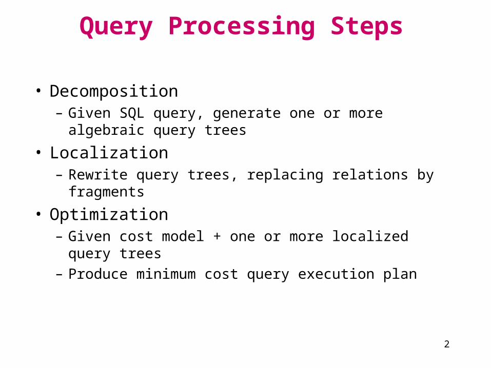
Query Processing Steps

• Decomposition – Given SQL query, generate one or more algebraic query

trees

• Localization– Rewrite query trees, replacing relations by fragments

• Optimization– Given cost model + one or more localized query trees

– Produce minimum cost query execution plan

3

Decomposition

• Same as in a centralized DBMS• Normalization (usually into relational algebra)

Select A,C from R Natural Join S where (R.B = 1 and S.D = 2) or (R.C > 3 and S.D = 2)

(R.B = 1 v R.C > 3) (S.D = 2)

R S

Conjunctive

normalform

4

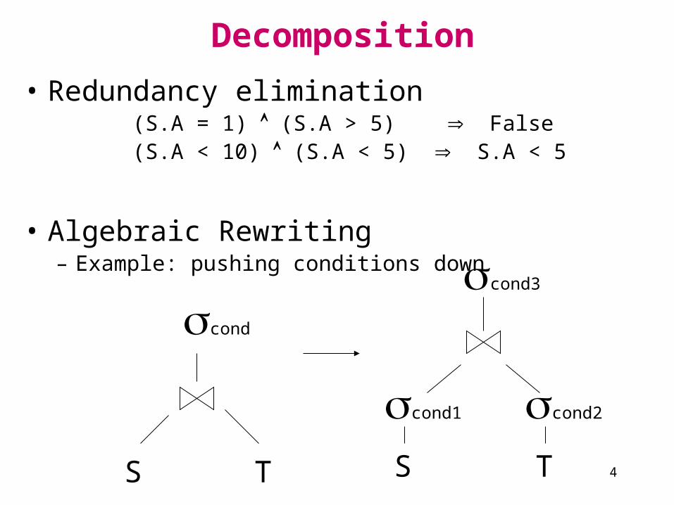
• Redundancy elimination (S.A = 1) (S.A > 5) False (S.A < 10) (S.A < 5) S.A < 5

• Algebraic Rewriting– Example: pushing conditions down

Decomposition

S ST T

cond

cond1 cond2

cond3

5

Localization Steps

1. Start with query tree

2. Replace relations by fragments

3. Push up & , down (rewriting rules)

4. Simplify – eliminating unnecessary operations

Note: To denote fragments in query trees

[R: cond]

Relation that fragment belongs to Condition its tuples satisfy

6

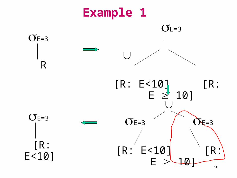
Example 1

E=3

R

E=3

[R: E<10] [R: E 10]

E=3 E=3

[R: E<10] [R: E 10]

E=3

[R: E<10]

7

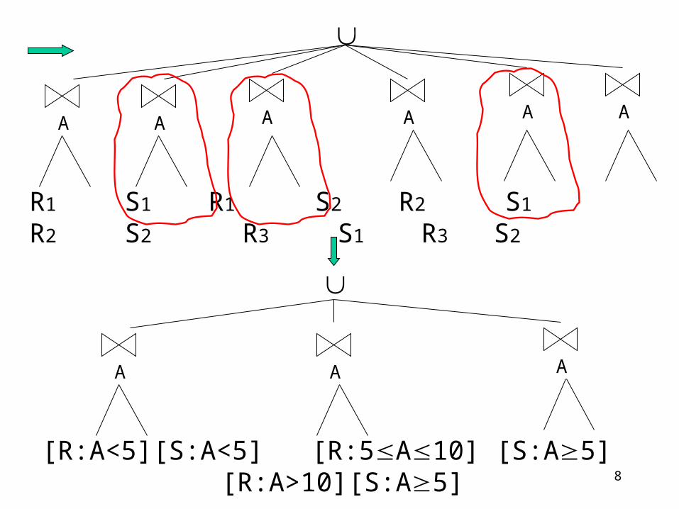
Example 2

R S

A

[R: A<5] [R: 5 A 10] [R: A>10]

[S: A<5] [S: A 5]

A

R1 R2 R3 S1 S2

8

R1 S1 R1 S2 R2 S1 R2 S2 R3 S1 R3

S2

AA AAA A

[R:A<5][S:A<5] [R:5A10] [S:A5] [R:A>10][S:A5]

AAA

9

Rules for Horiz. Fragmentation C1[R: C2] [R: C1 C2]• [R: False] Ø• [R: C1] [S: C2] [R S: C1 C2 R.A = S.A]

• In Example 1:

E=3[R2: E 10] [R: E=3 E 10] [R: False] Ø• In Example 2: [R: A<5] [S: A 5] [R S: R.A < 5 S.A 5 R.A = S.A] [R S: False] Ø

A A

A

A

A

10

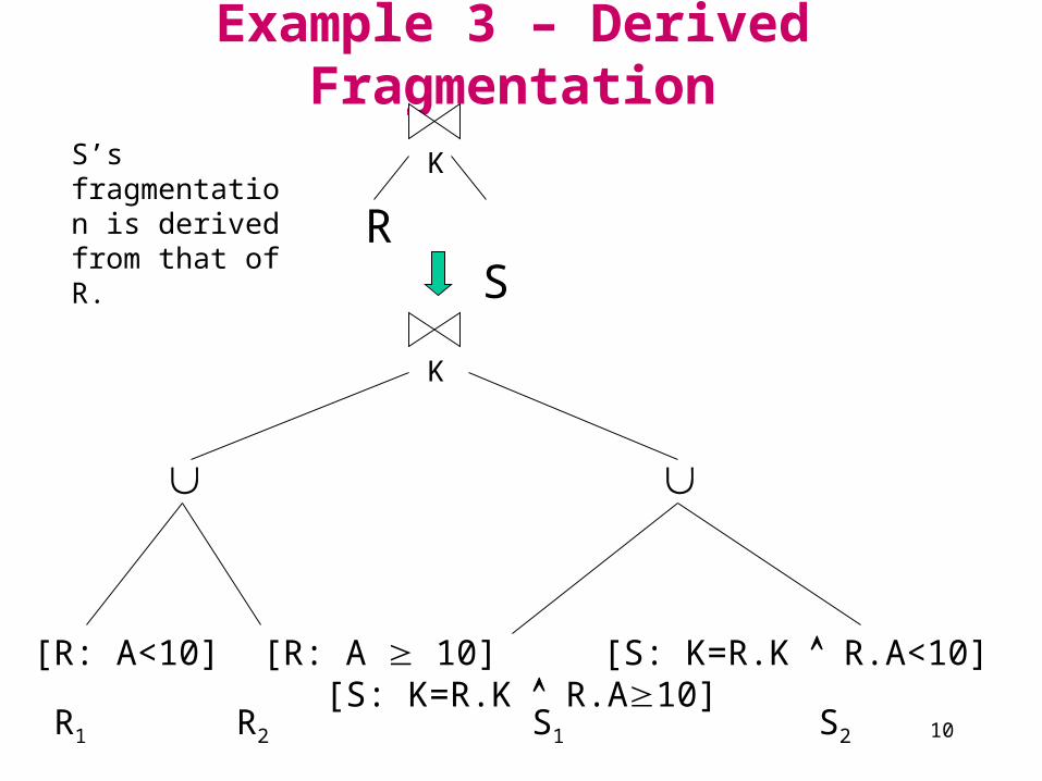
Example 3 – Derived Fragmentation

R S

KS’s fragmentation is derived from that of R.

[R: A<10] [R: A 10] [S: K=R.K R.A<10] [S: K=R.K R.A10]

K

R1 R2 S2S1

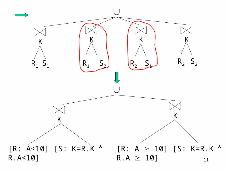
11

KK KK

R1 S1 R1 S2 S1S2R2

R2

KK

[R: A<10] [S: K=R.K R.A<10] [R: A 10] [S: K=R.K R.A 10]

12

Example 4 – Vertical Fragmentation

A

R

A

R1(K,A,B) R2(K,C,D)

K

A

K,A K,A

R1(K,A,B) R2(K,C,D)

KA

R1(K,A,B)

13

Rule for Vertical Fragmentation

• Given vertical fragmentation of R(A):

Ri = Ai(R), Ai A

• For any B A:

B (R) = B [ Ri | B Ai Ø]i

14

Parallel/Distributed Query Operations

• Sort– Basic sort

– Range-partitioning sort

– Parallel external sort-merge

• Join– Partitioned join

– Asymmetric fragment and replicate join

– General fragment and replicate join

– Semi-join programs

• Aggregation and duplicate removal

15

Parallel/distributed sort

• Input: relation R on– single site/disk

– fragmented/partitioned by sort attribute

– fragmented/partitioned by some other attribute

• Output: sorted relation R– single site/disk

– individual sorted fragments/partitions

16

Basic sort• Given R(A,…) range partitioned on attribute A, sort R

on A

• Each fragment is sorted independently• Results shipped elsewhere if necessary

7

3

11

17

14

27

2210 20

3

7

11

14

17

22

2710 20

17

Range partitioning sort

• Given R(A,….) located at one or more sites, not fragmented on A, sort R on A

• Algorithm: range partition on A and then do basic sort

R1s

R2s

R3s

a0

Local sort

Local sort

Local sort

RaR1

R2

R3

Rb Result

a1

18

Selecting a partitioning vector

• Possible centralized approach using a “coordinator”– Each site sends statistics about its fragment to coordinator

– Coordinator decides # of sites to use for local sort

– Coordinator computes and distributes partitioning vector

• For example, – Statistics could be (min sort key, max sort key, # of tuples)

– Coordinator tries to choose vector that equally partitions relation

19

Example

• Coordinator receives:– From site 1: Min 5, Max 9, 10 tuples– From site 2: Min 7, Max 16, 10 tuples

• Assume sort keys distributed uniformly within [min,max] in each fragment

• Partition R into two fragments

5 10 15 20k0

What is k0?

20

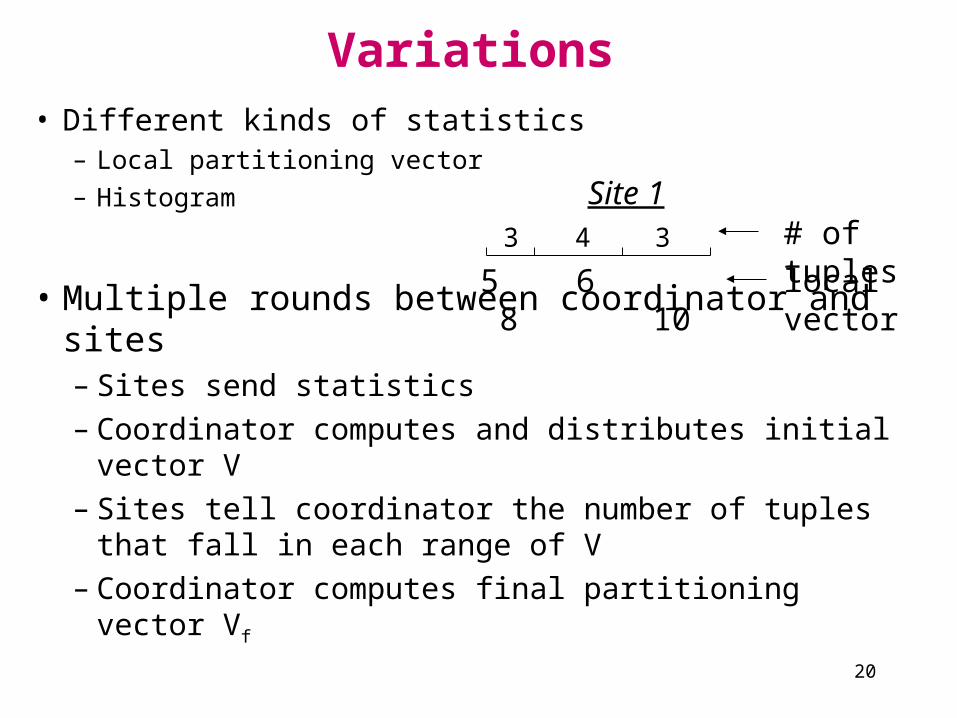
Variations

• Different kinds of statistics– Local partitioning vector

– Histogram

• Multiple rounds between coordinator and sites– Sites send statistics– Coordinator computes and distributes initial vector V– Sites tell coordinator the number of tuples that fall in

each range of V

– Coordinator computes final partitioning vector Vf

5 6 8 10

3 4 3

local vector

# of tuplesSite 1

21

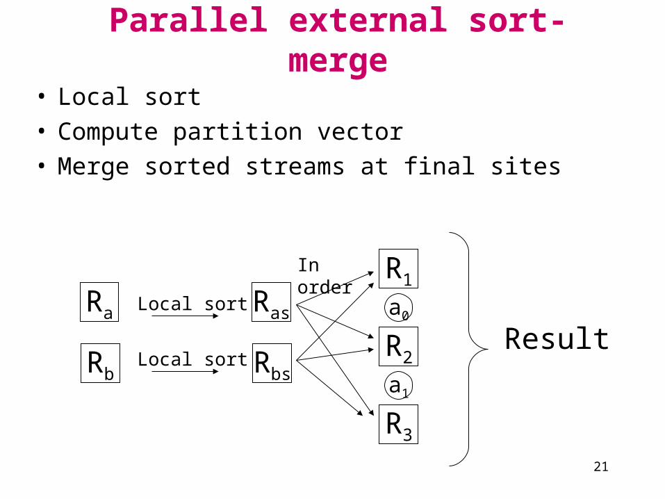
Parallel external sort-merge

• Local sort• Compute partition vector• Merge sorted streams at final sites

Ra

Rb

Local sort

Local sort

Ras

Rbs

R1

R2

R3

a0

a1

In order

Result

22

Parallel/distributed join

Input: Relations R, S

May or may not be partitioned

Output:R S

Result at one or more sites

23

Partitioned Join

Local join

Result f(A)

Ra

Rb

R1

f(A)

R2

R3

S1

S2

S3

Sa

Sb

Note: Works only for equi-joins

Join attribute A

24

Partitioned Join

• Same partition function (f) for both relations• f can be range or hash partitioning• Any type of local join (nested-loop, hash, merge, etc.)

can be used• Several possible scheduling options. Example:

– partition R; partition S; join

– partition R; build local hash table for R; partition S and join

• Good partition function important– Distribute join load evenly among sites

25

Asymmetric fragment + replicate join

Local join

Result

Ra

Rb

R1

f

R2

R3

S Sa

Sb

Join attribute A

Partition functionunion

• Any partition function f can be used (even round-robin)

• Can be used for any kind of join, not just equi-joins

S

S

26

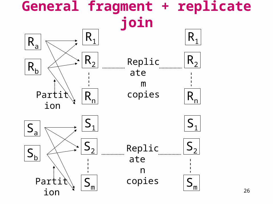
General fragment + replicate join

Ra

Rb

R1

R2

RnPartition

R1

R2

Rn

Replicate m

copies

Sa

Sb

S1

S2

SmPartition

S1

S2

Sm

Replicate n copies

27

All n x m pairings ofR,S fragments

R1 S1

R2 S1

Rn S1

R1 Sm

R2 Sm

Rn Sm

Result

•Asymmetric F+R join is a special case of general F+R.

•Asymmetric F+R is useful when S is small.

28

• Used to reduce communication traffic during join processing

• R S = (R S) S

= R (S R)

= (R S) (S R)

Semi-join programs

29

Example

A(S) = [2,10,25,30]

b

a2

10

c

d

25

30

y

x3

10

z

w

15

25

32 x

A B A C

S R

R S =

w

y10

25

Compute

S (R S)

• Using semi-join, communication cost = 4 A + 2 (A + C) + result

• Directly joining R and S, communication cost = 4 (A + B) + result

30

Comparing communication costs

• Say R is the smaller of the two relations R and S

• (R S) S is cheaper than R S if

size (A(S)) + size (R S) < size (R)

• Similar comparisons for other types of semi-joins

• Common implementation trick:– Encode AS (or AR) as a bit vector

– 1 bit per domain of attribute A

0 0 1 1 0 1 0 0 0 0 1 0 1 0 0

31

n-way joins

• To compute R S T– Semi-join program 1: R’ S’ T

where R’ = R S & S’ = S T– Semi-join program 2: R’’ S’ T

where R’’ = R S’ & S’ = S T– Several other options (Bernstein’s reducers)

• In general, number of options is exponential in the number of relations

32

Other operations

• Duplicate elimination– Sort first (in parallel), then eliminate duplicates in the result

– Partition tuples (range or hash) and eliminate duplicates locally

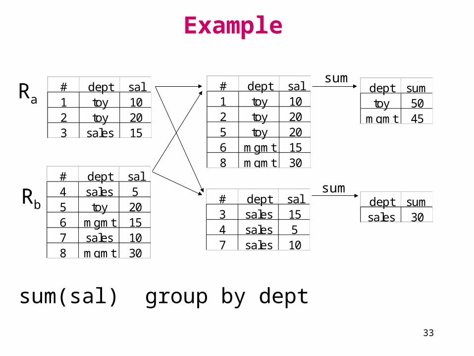
• Aggregates– Partition by grouping attributes; compute aggregates locally

at each site

33

Example

# dept sal1 toy 102 toy 203 sales 15

# dept sal4 sales 55 toy 206 mgmt 157 sales 108 mgmt 30

sum(sal) group by dept

# dept sal1 toy 102 toy 205 toy 206 mgmt 158 mgmt 30

# dept sal3 sales 154 sales 57 sales 10

dept sumtoy 50mgmt 45

dept sumsales 30

sum

sum

Ra

Rb

34

Example

# dept sal1 toy 102 toy 203 sales 15

# dept sal4 sales 55 toy 206 mgmt 157 sales 108 mgmt 30

dept sumtoy 50mgmt 45

dept sumsales 30

sum

sum

dept sumtoy 30toy 20mgmt 45

dept sumsales 15sales 15

sum

sum

Ra

Rb

Aggregate during partitioning to reduce communication cost

Does this work for all kinds of aggregates?

35

Query Optimization

• Generate query execution plans (QEPs)• Estimate cost of each QEP ($,time,…)• Choose minimum cost QEP

• What’s different for distributed DB?– New strategies for some operations (semi-join, range-

partitioning sort,…)

– Many ways to assign and schedule processors

– Some factors besides number of IO’s in the cost model

36

Cost estimation

• In centralized systems - estimate sizes of intermediate relations

• For distributed systems– Transmission cost/time may dominate

– Account for parallelism

– Data distribution and result re-assembly cost/time

Work at site

Work at site

T1 T2 answer

100 IOs

50 IOs

70 IOs

20 IOs

Plan APlan B

37

Optimization in distributed DBs

• Two levels of optimization• Global optimization

– Given localized query and cost function

– Output optimized (min. cost) QEP that includes relational and communication operations on fragments

• Local optimization– At each site involved in query execution

– Portion of the QEP at a given site optimized using techniques from centralized DB systems

38

Search strategies

1. Exhaustive (with pruning)

2. Hill climbing (greedy)

3. Query separation

39

• A fixed set of techniques for each relational operator• Search space = “all” possible QEPs with this set of

techniques• Prune search space using heuristics• Choose minimum cost QEP from rest of search

space

Exhaustive with Pruning

40

R S T

R S RT S R S T T S TR

(S R) T (T S) R

|R|>|S|>|T| R S TA B

2 1 2 1

2

Prune because cross-product not necessary

Prune because larger relation first

1

Ship S to R

Semi-join Ship T to S

Semi-join

Example

41

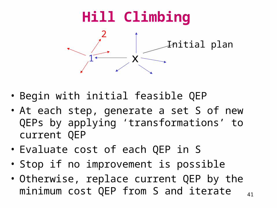
Hill Climbing

• Begin with initial feasible QEP• At each step, generate a set S of new QEPs by applying

‘transformations’ to current QEP• Evaluate cost of each QEP in S• Stop if no improvement is possible• Otherwise, replace current QEP by the minimum cost

QEP from S and iterate

xInitial plan

1

2

42

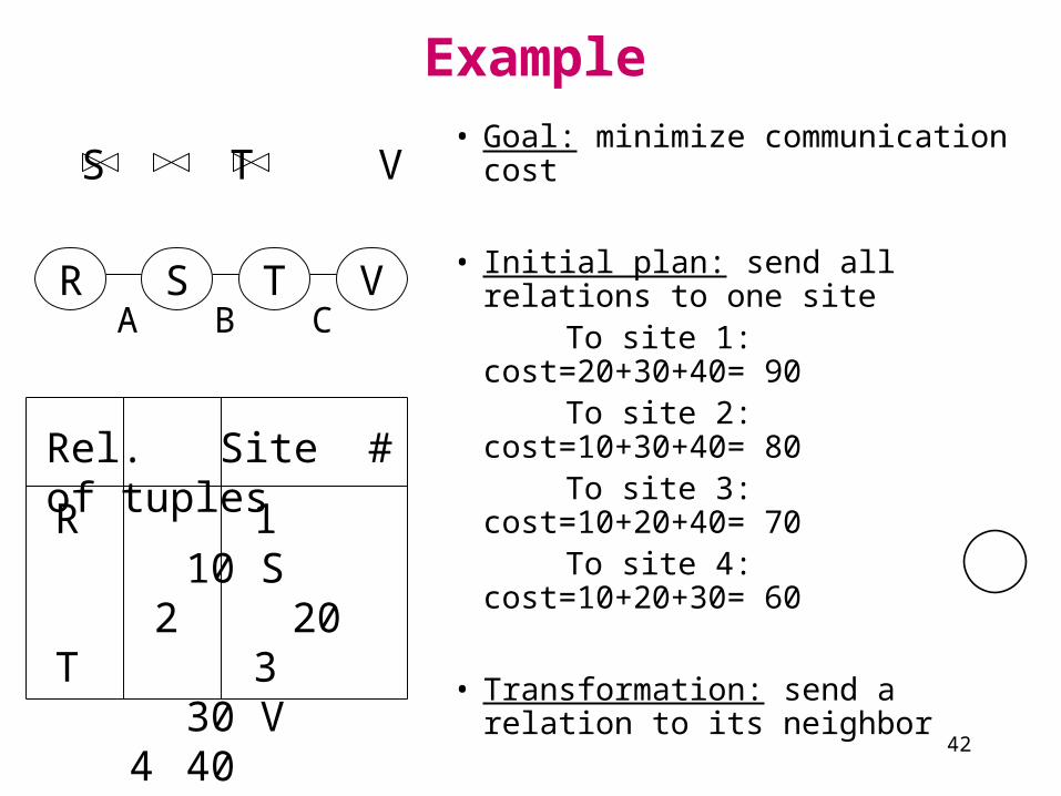
R S T VA B C

Example

R S T V

R 1 10 S 2 20 T 3

30 V 4 40

Rel. Site # of tuples

• Goal: minimize communication cost

• Initial plan: send all relations to one site

To site 1: cost=20+30+40= 90 To site 2: cost=10+30+40= 80 To site 3: cost=10+20+40= 70 To site 4: cost=10+20+30= 60

• Transformation: send a relation to its neighbor

43

• Initial feasible plan

P0: R (1 4); S (2 4); T (3 4)

Compute join at site 4

• Assume following sizes: R S 20

S T 5

T V 1

Local search

44

4

1 2SR

10 20

cost = 30

4

1 2

R S

R10

20 cost = 30

4

1 2

S R

S20

20

cost = 40

No change

Worse

45

4

2 3

TS 30

20

cost = 50T

4

2 3

T S 30

5 cost = 35

4

2 3

S T

S20

5

cost = 25

Improvement

Improvement

46

• P1: S (2 3); R (1 4); (3 4)

where = S T

Compute answer at site 4• Now apply same transformation to R and

Next iteration

4

1 3

R

4

1 3

R

4

1 3R

R