Distributed Database Systems COP5711. What is a Distributed Database System ? A distributed database...
146
Distributed Database Systems COP5711
-
date post
19-Dec-2015 -
Category
Documents
-
view
261 -
download
9
Transcript of Distributed Database Systems COP5711. What is a Distributed Database System ? A distributed database...
Distributed Database Systems
COP5711
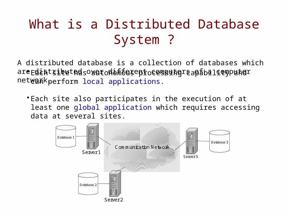
What is a Distributed Database System ?
A distributed database is a collection of databases which are distributed over different computers of a computer network.•Each site has autonomous processing capability and can
perform local applications.
•Each site also participates in the execution of at least one global application which requires accessing data at several sites.
Communication NetworkServer 1
Database 1
Server 2
Database 2
Server 3
Database 3
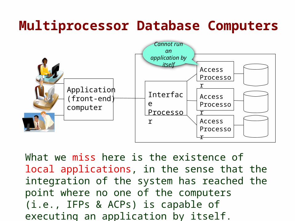
Multiprocessor Database Computers
Application (front-end) computer
Interface Processor
Access Processor
Access Processor
Access Processor
What we miss here is the existence of local applications, in the sense that the integration of the system has reached the point where no one of the computers (i.e., IFPs & ACPs) is capable of executing an application by itself.
Cannot run an
application by itself
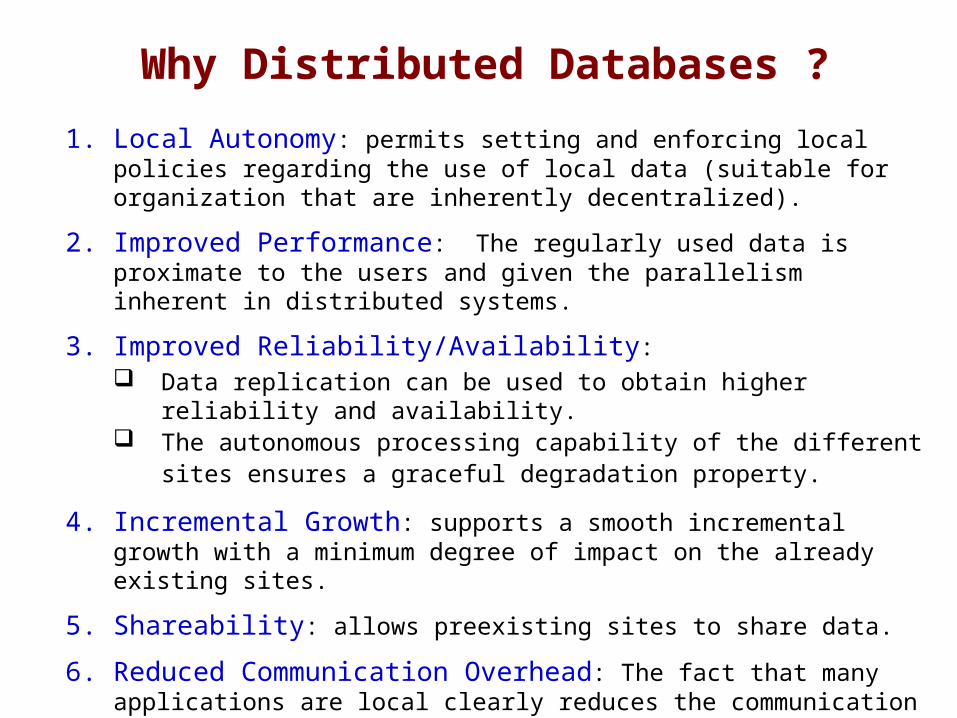
Why Distributed Databases ?
1. Local Autonomy: permits setting and enforcing local policies regarding the use of local data (suitable for organization that are inherently decentralized).
2. Improved Performance: The regularly used data is proximate to the users and given the parallelism inherent in distributed systems.
3. Improved Reliability/Availability: Data replication can be used to obtain higher reliability and
availability. The autonomous processing capability of the different sites
ensures a graceful degradation property.
4. Incremental Growth: supports a smooth incremental growth with a minimum degree of impact on the already existing sites.
5. Shareability: allows preexisting sites to share data.
6. Reduced Communication Overhead: The fact that many applications are local clearly reduces the communication overhead with respect to centralized databases.
Disadvantages of DDBSs
Cost: replication of effort (manpower).
Security: More difficult to control
Complexity:
• The possible duplication is mainly due to reliability and efficiency considerations. Data redundancy, however, complicates update operations.
• If some sites fail while an update is being executed, the system must make sure that the effects will be reflected on the data residing at the failing sites as soon as the system can recover from the failure.
• The synchronization of transactions on multiple sites is considerably harder than for a centralized system.
Distributed DBMS Architecture
NetworkTransparancy
• The user should be protected from the operational details of the network.
• It is desirable to hide even the existence of the network, if possible. Location transparency: The command used
is independent of the system on which the data is stored.
Naming transparency: a unique name is provided for each object in the database.
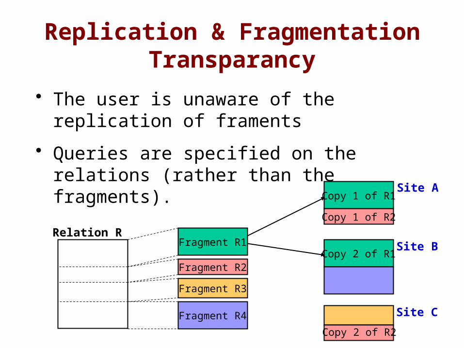
Replication & Fragmentation Transparancy
• The user is unaware of the replication of framents
• Queries are specified on the relations (rather than the fragments).
Fragment R1
Fragment R2
Fragment R3
Fragment R4
Copy 2 of R1
Copy 1 of R1
Copy 1 of R2
Relation R
Copy 2 of R2
Site A
Site B
Site C
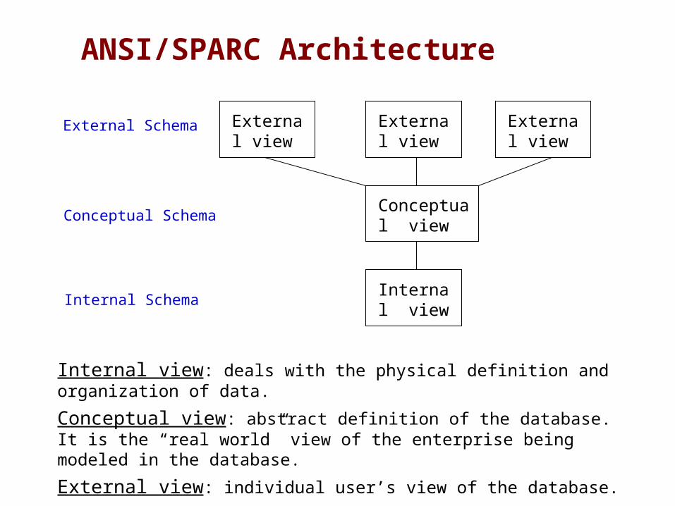
ANSI/SPARC Architecture
External view
External view
External view
Conceptual view
Internal view
External Schema
Conceptual Schema
Internal Schema
Internal view: deals with the physical definition and organization of data.
Conceptual view: abstract definition of the database. It is the “real world” view of the enterprise being modeled in the database.
External view: individual user’s view of the database.
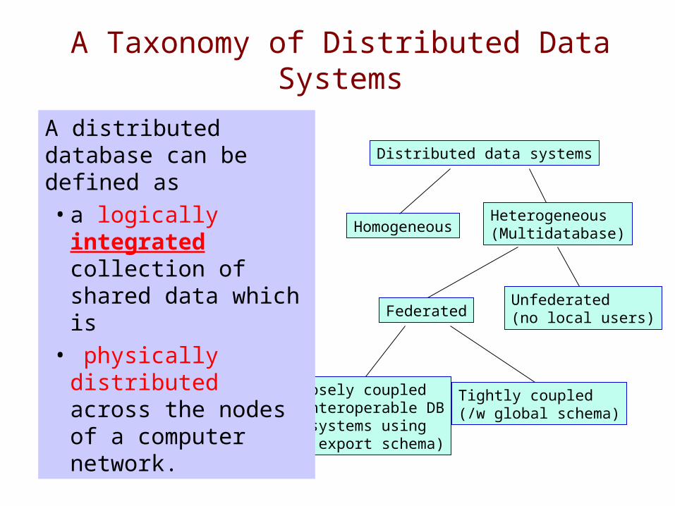
A Taxonomy of Distributed Data Systems
Distributed data systems
HomogeneousHeterogeneous(Multidatabase)
Unfederated(no local users)Federated
Loosely coupled(interoperable DB systems using export schema)
Tightly coupled(/w global schema)
A distributed database can be defined as• a logically
integrated collection of shared data which is
• physically distributed across the nodes of a computer network.
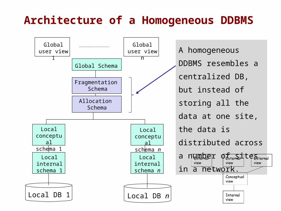
Architecture of a Homogeneous DDBMS
Global user view 1
Global Schema
Global user view n
Fragmentation Schema
Local conceptu
al schema 1
Local internal
schema 1
Local DB 1
Allocation Schema
Local conceptu
al schema n
Local internal
schema n
Local DB n
A homogeneous
DDBMS resembles a
centralized DB, but
instead of storing all
the data at one site,
the data is
distributed across a
number of sites in a
network.
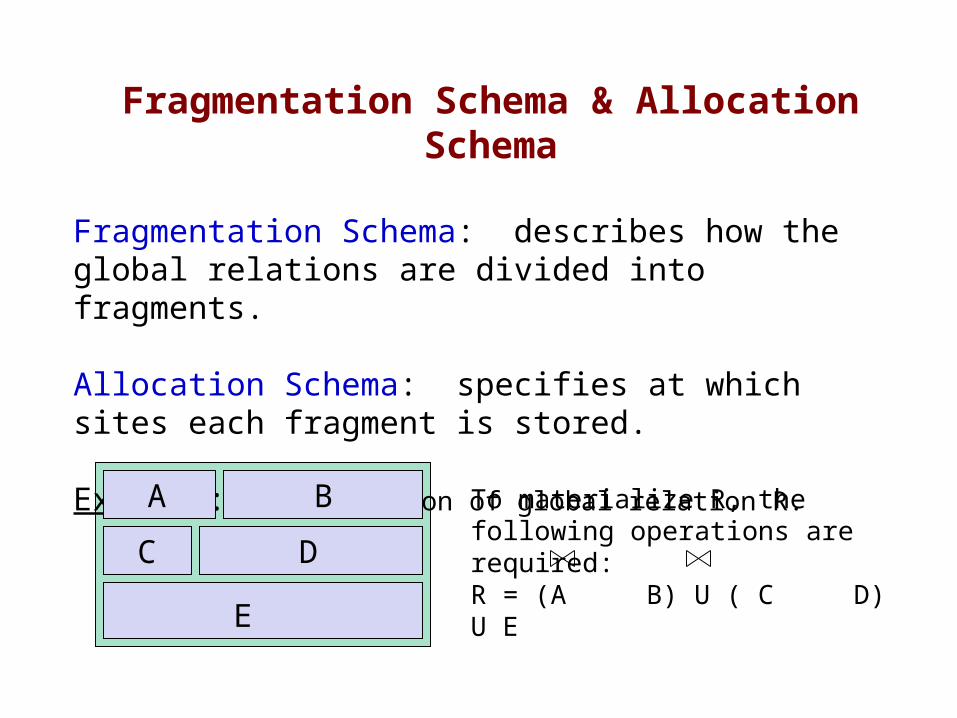
Fragmentation Schema & Allocation Schema
Fragmentation Schema: describes how the global relations are divided into fragments.
Allocation Schema: specifies at which sites each fragment is stored.
Example: Fragmentation of global relation R.A B
C D
E
To materialize R, the following operations are required:R = (A B) U ( C D) U E
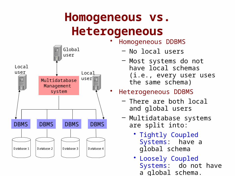
Homogeneous vs. Heterogeneous
• Homogeneous DDBMS– No local users– Most systems do not have
local schemas (i.e., every user uses the same schema)
• Heterogeneous DDBMS– There are both local and
global users– Multidatabase systems are
split into:• Tightly Coupled Systems:
have a global schema• Loosely Coupled
Systems: do not have a global schema.
MultidatabaseManagement
system
DBMSDBMS DBMS DBMS
Database 1 Database 2 Database 3 Database 4
Globaluser
Localuser
Localuser
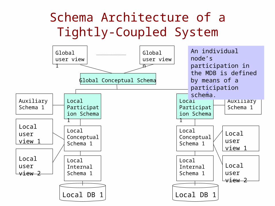
Schema Architecture of a Tightly-Coupled System
Global user view 1
Global user view n
Global Conceptual Schema
Local Participation Schema 1
Auxiliary Schema 1
Local Conceptual Schema 1
Local user view 1
Local user view 2
Local Internal Schema 1
Local DB 1
Local Participation Schema 1
Auxiliary Schema 1
Local Conceptual Schema 1
Local user view 1
Local user view 2
Local Internal Schema 1
Local DB 1
An individual node’s participation in the MDB is defined by means of a participation schema.
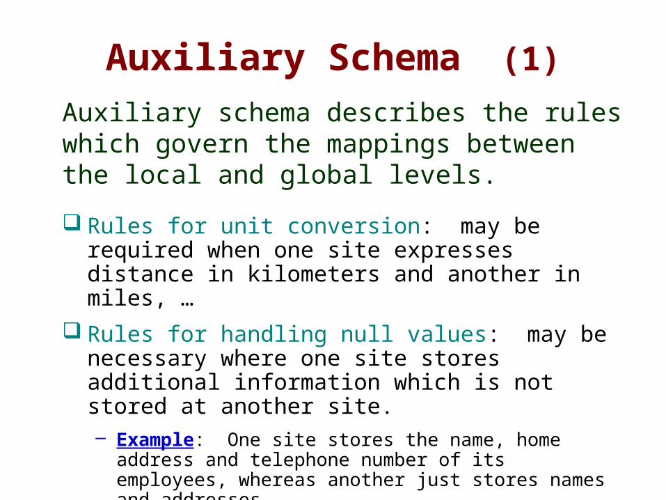
Auxiliary Schema (1)
Rules for unit conversion: may be required when one site expresses distance in kilometers and another in miles, …
Rules for handling null values: may be necessary where one site stores additional information which is not stored at another site.– Example: One site stores the name, home address
and telephone number of its employees, whereas another just stores names and addresses.
Auxiliary schema describes the rules which govern the mappings between the local and global levels.
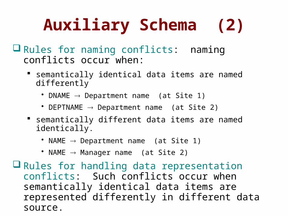
Auxiliary Schema (2) Rules for naming conflicts: naming conflicts occur
when: semantically identical data items are named differently
• DNAME Department name (at Site 1)
• DEPTNAME Department name (at Site 2)
semantically different data items are named identically.• NAME Department name (at Site 1)
• NAME Manager name (at Site 2)
Rules for handling data representation conflicts: Such conflicts occur when semantically identical data items are represented differently in different data source. Example: Data represented as a character string in one
database may be represented as a real number in the other database.
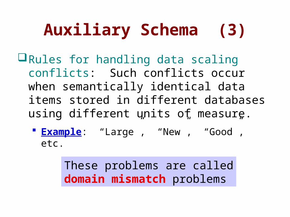
Auxiliary Schema (3)
Rules for handling data scaling conflicts: Such conflicts occur when semantically identical data items stored in different databases using different units of measure. Example: “Large”, “New”, “Good”, etc.
These problems are calleddomain mismatch problems
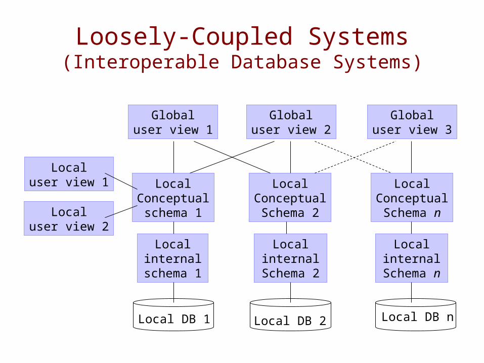
Loosely-Coupled Systems(Interoperable Database Systems)
Globaluser view 1
Globaluser view 2
Globaluser view 3
LocalConceptualschema 1
Localinternal
schema 1
Localinternal
Schema 2
LocalConceptualSchema 2
Localinternal
Schema n
LocalConceptualSchema n
Local DB nLocal DB 2Local DB 1
Localuser view 1
Localuser view 2
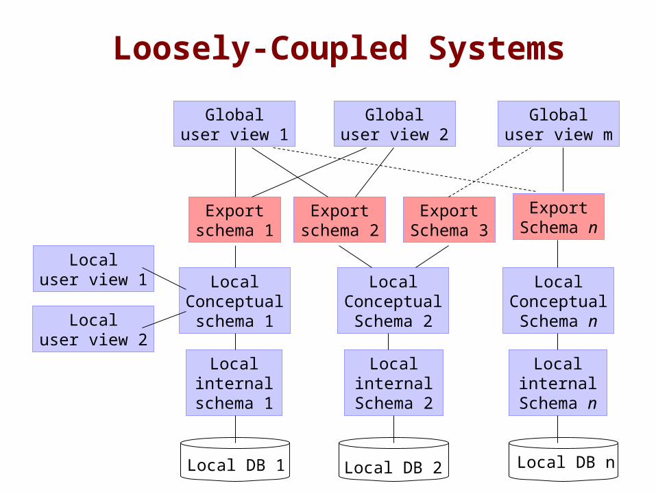
Loosely-Coupled Systems
Globaluser view 1
Globaluser view 2
Globaluser view m
LocalConceptualschema 1
Localinternal
schema 1
Localinternal
Schema 2
LocalConceptualSchema 2
Localinternal
Schema n
LocalConceptualSchema n
Local DB nLocal DB 2Local DB 1
Localuser view 1
Localuser view 2
Exportschema 2
ExportSchema 3
ExportSchema n
Exportschema 1
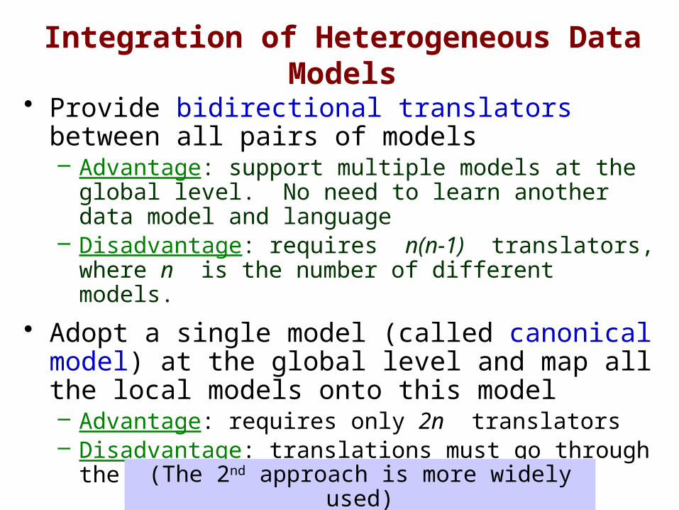
Integration of Heterogeneous Data Models
• Provide bidirectional translators between all pairs of models– Advantage: support multiple models at the global
level. No need to learn another data model and language
– Disadvantage: requires n(n-1) translators, where n is the number of different models.
• Adopt a single model (called canonical model) at the global level and map all the local models onto this model– Advantage: requires only 2n translators– Disadvantage: translations must go through the
global model.(The 2nd approach is more widely used)
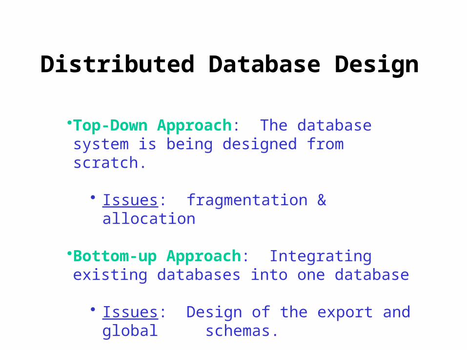
Distributed Database Design
•Top-Down Approach: The database system is being designed from scratch.
• Issues: fragmentation & allocation
•Bottom-up Approach: Integrating existing databases into one database
• Issues: Design of the export and global schemas.
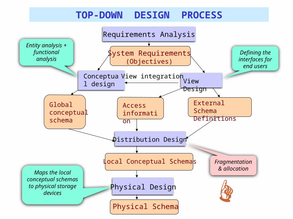
Requirements Analysis
System Requirements(Objectives)
Conceptual design View
Design
Global conceptual schema
Access information
External Schema Definitions
Distribution Design
Local Conceptual Schemas
Physical Design
Physical Schema
View integration
TOP-DOWN DESIGN PROCESS
Fragmentation &
allocation
Defining the interfaces for
end users
Entity analysis + functional
analysis
Maps the local conceptual schemas to
physical storage devices
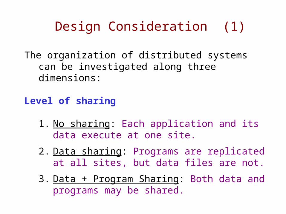
Design Consideration (1)
The organization of distributed systems can be investigated along three dimensions:
Level of sharing
1. No sharing: Each application and its data execute at one site.
2. Data sharing: Programs are replicated at all sites, but data files are not.
3. Data + Program Sharing: Both data and programs may be shared.
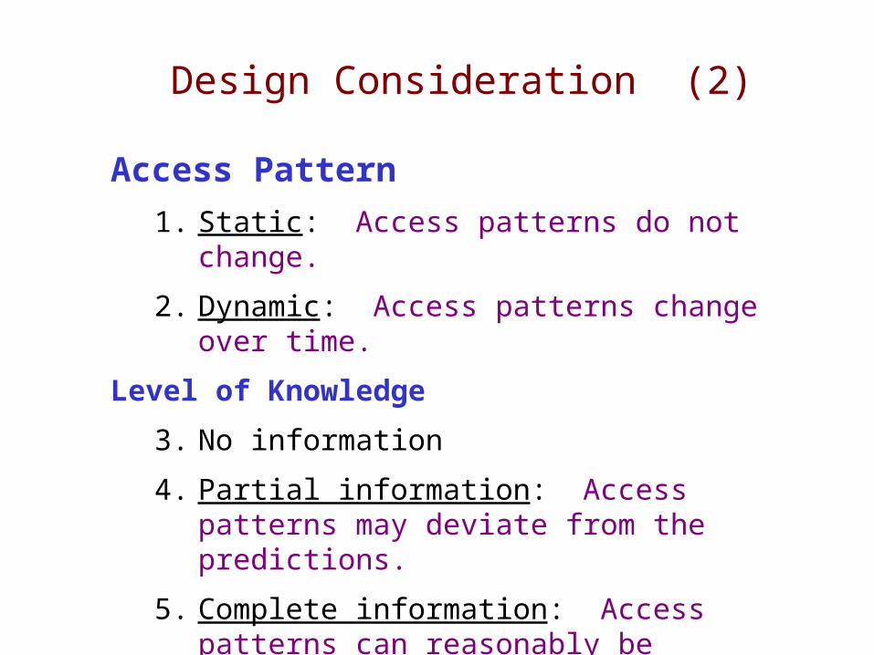
Access Pattern
1. Static: Access patterns do not change.
2. Dynamic: Access patterns change over time.
Level of Knowledge
3. No information
4. Partial information: Access patterns may deviate from the predictions.
5. Complete information: Access patterns can reasonably be predicted.
Design Consideration (2)
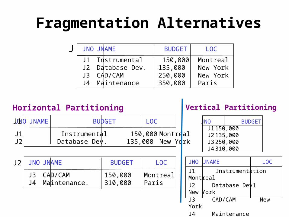
Fragmentation Alternatives
Horizontal Partitioning
JNO JNAME BUDGET LOC
J1 Instrumental 150,000 MontrealJ2 Database Dev. 135,000 New York
J1
JNO JNAME BUDGET LOC
J3 CAD/CAM 150,000 MontrealJ4 Maintenance. 310,000 Paris
J2
JNO JNAME BUDGET LOC
J1 Instrumental 150,000 MontrealJ2 Database Dev. 135,000 New YorkJ3 CAD/CAM 250,000 New YorkJ4 Maintenance 350,000 Paris
J
Vertical Partitioning
JNO BUDGET J1 150,000 J2 135,000 J3 250,000 J4 310,000
JNO JNAME LOC
J1 Instrumentation MontrealJ2 Database Devl New YorkJ3 CAD/CAM New YorkJ4 Maintenance Paris
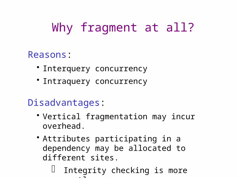
Why fragment at all?
Reasons:• Interquery concurrency• Intraquery concurrency
Disadvantages:• Vertical fragmentation may incur overhead.• Attributes participating in a dependency
may be allocated to different sites.
Integrity checking is more costly.
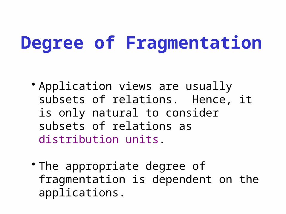
Degree of Fragmentation
• Application views are usually subsets of relations. Hence, it is only natural to consider subsets of relations as distribution units.
• The appropriate degree of fragmentation is dependent on the applications.

Correctness Rules
• Vertical Partitioning• Lossless
decomposition• Dependency
preservation
• Horizontal Partitioning
• Disjoint fragments
Allocation Alternatives
•Partitioning: No replication
•Partial Replication: Some fragments are replicated
•Full Replication: Database exists in its entirety at each site
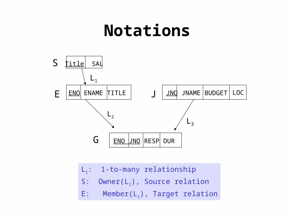
Notations
Title SAL
ENO ENAME TITLE
S
E
L1
JNO JNAME BUDGETJ LOC
L2L3
ENO JNO RESP DURG
L1: 1-to-many relationship
S: Owner(L1), Source relation
E: Member(L1), Target relation
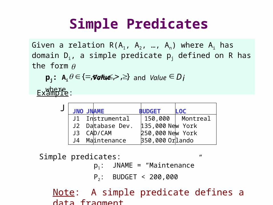
Simple PredicatesGiven a relation R(A1, A2, …, An) where Ai has domain Di, a simple predicate pj defined on R has the form
pj: Ai Value
where
},,,,,{ and Value Di
Example:
JNO JNAME BUDGET LOCJ1 Instrumental 150,000 MontrealJ2 Database Dev. 135,000 New YorkJ3 CAD/CAM 250,000 New YorkJ4 Maintenance 350,000 Orlando
J
Simple predicates: p1: JNAME = “Maintenance”
P2: BUDGET < 200,000
Note: A simple predicate defines a data fragment
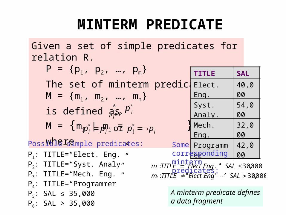
Given a set of simple predicates for relation R.
P = {p1, p2, …, pm}
The set of minterm predicatesM = {m1, m2, …, mn}
is defined as
M = {mi | mi = }where
MINTERM PREDICATE
*
jp
Pp j
jjj pppp *j
* or
TITLE SAL
Elect. Eng. 40,000
Syst. Analy. 54,000
Mech. Eng. 32,000
Programmer 42,000
Possible simple predicates:
P1: TITLE=“Elect. Eng.”P2: TITLE=“Syst. Analy”P3: TITLE=“Mech. Eng.”P4: TITLE=“Programmer”P5: SAL ≤ 35,000P6: SAL > 35,000
Some corresponding minterm predicates:
000,30".":
000,30.".":
2
1
SALEngElectTITLEm
SALEngElectTITLEm
A minterm predicate definesa data fragment
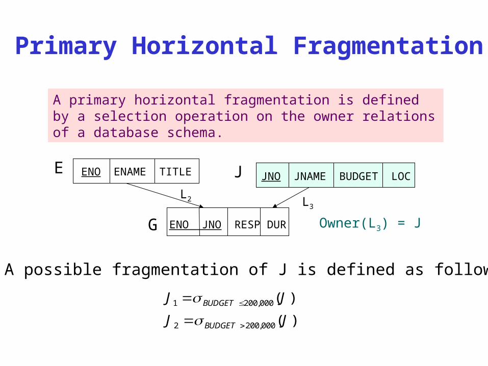
Primary Horizontal Fragmentation
A primary horizontal fragmentation is defined by a selection operation on the owner relations of a database schema.
ENO ENAME TITLE JNO JNAME BUDGET LOCE J
ENO JNO RESP DURG
L2 L3
Owner(L3) = J
A possible fragmentation of J is defined as follows:
)(
)(
000,2002
000,2001
JJ
JJ
BUDGET
BUDGET
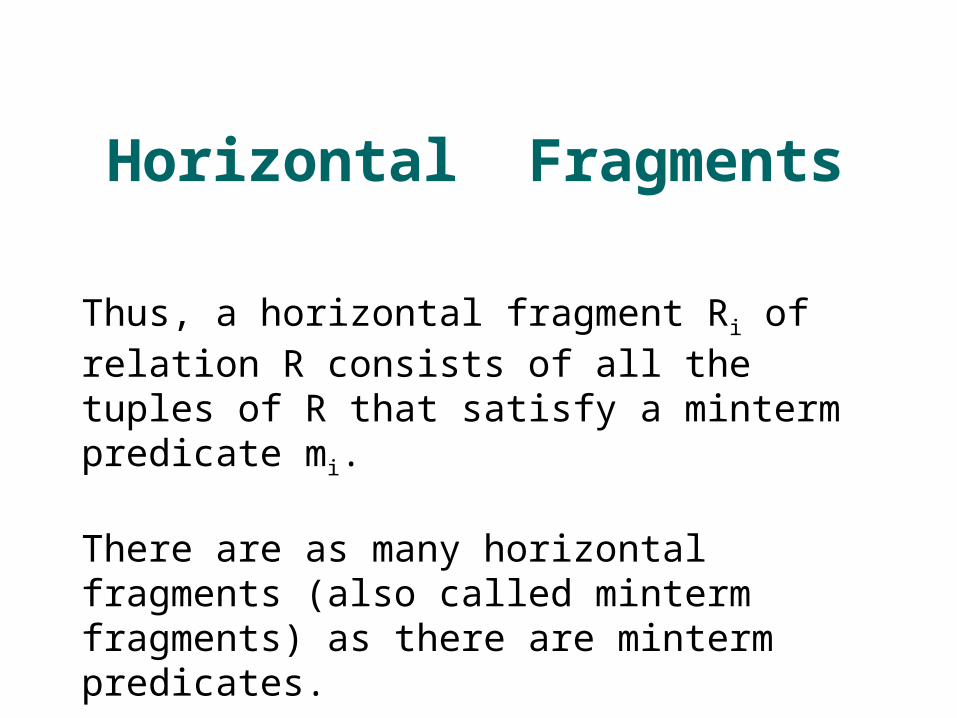
Horizontal Fragments
Thus, a horizontal fragment Ri of relation R consists of all the tuples of R that satisfy a minterm predicate mi.
There are as many horizontal fragments (also called minterm fragments) as there are minterm predicates.
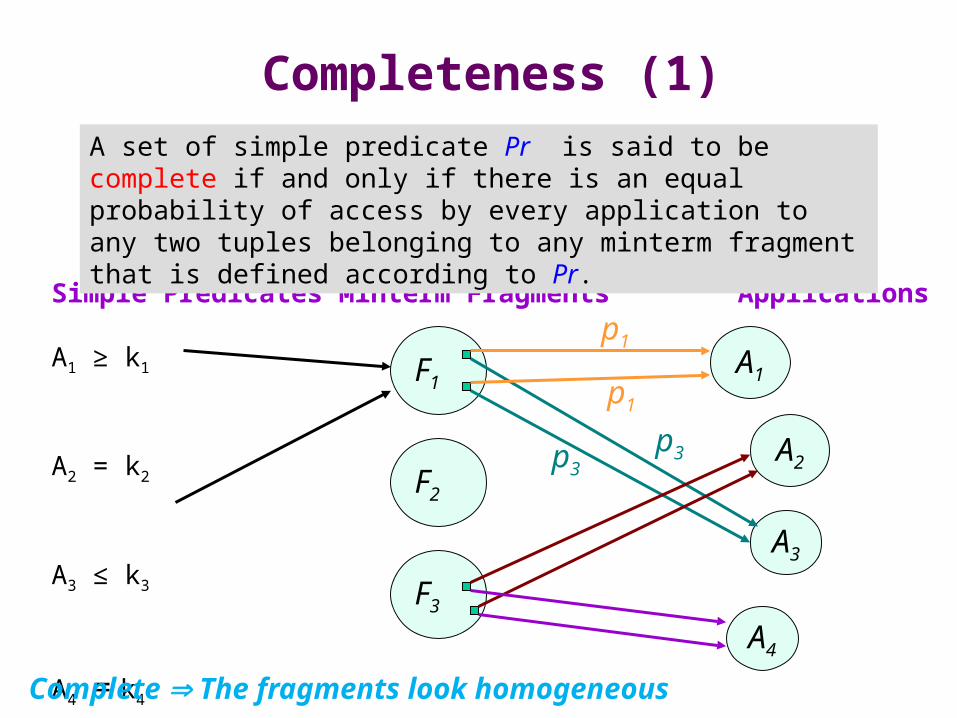
Simple Predicates Minterm Fragments Applications
A1 ≥ k1
A2 = k2
A3 ≤ k3
A4 = k4
Completeness (1)A set of simple predicate Pr is said to be complete if and only if there is an equal probability of access by every application to any two tuples belonging to any minterm fragment that is defined according to Pr.
F1
F2
F3
A1
A2
A3
A4
p1
p1
p3p3
Complete The fragments look homogeneous
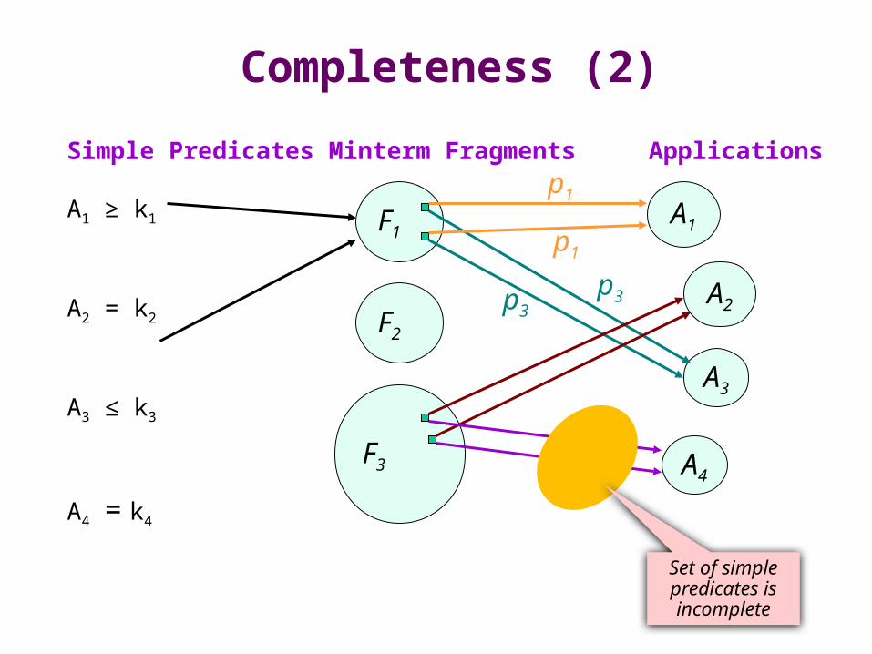
Simple Predicates Minterm Fragments Applications
A1 ≥ k1
A2 = k2
A3 ≤ k3
A4 = k4
Completeness (2)
F1
F2
F3
A1
A2
A3
A4
p1
p1
p3p3
p4
p5
Set of simple predicates is incomplete
F32
F31
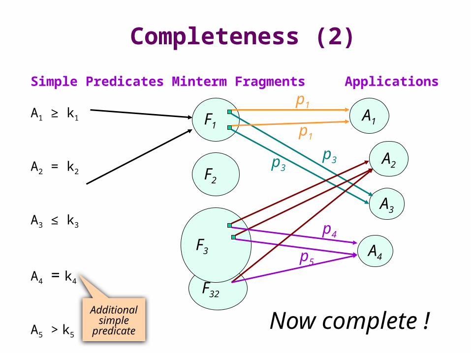
Simple Predicates Minterm Fragments Applications
A1 ≥ k1
A2 = k2
A3 ≤ k3
A4 = k4
A5 > k5
Completeness (2)
F1
F2
F3
A1
A2
A3
A4
p1
p1
p3p3
p4
p5
Additional simple
predicate Now complete !
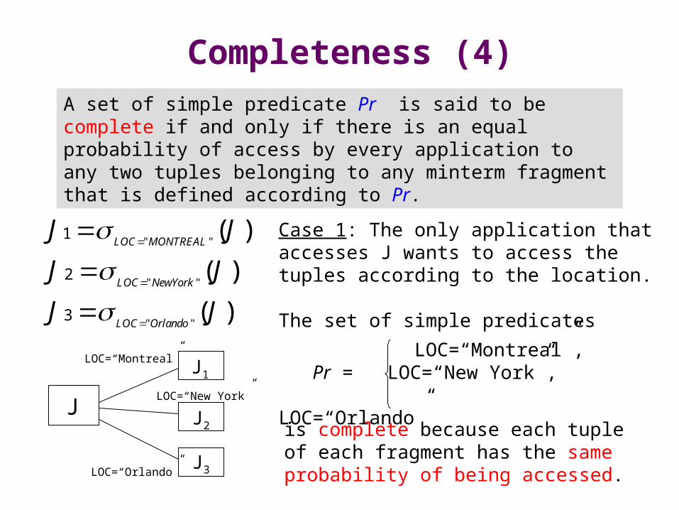
Completeness (4)A set of simple predicate Pr is said to be complete if and only if there is an equal probability of access by every application to any two tuples belonging to any minterm fragment that is defined according to Pr.
Case 1: The only application that accesses J wants to access the tuples according to the location.
The set of simple predicates
LOC=“Montreal”,Pr = LOC=“New York”,
LOC=“Orlando”
is complete because each tuple of each fragment has the same probability of being accessed.
" "
" "
" "
1
2
3
( )
( )
( )
LOC MONTREAL
LOC NewYork
LOC Orlando
J J
J J
J J
J
J1
J2
J3
LOC=“Montreal”
LOC=“New York”
LOC=“Orlando”
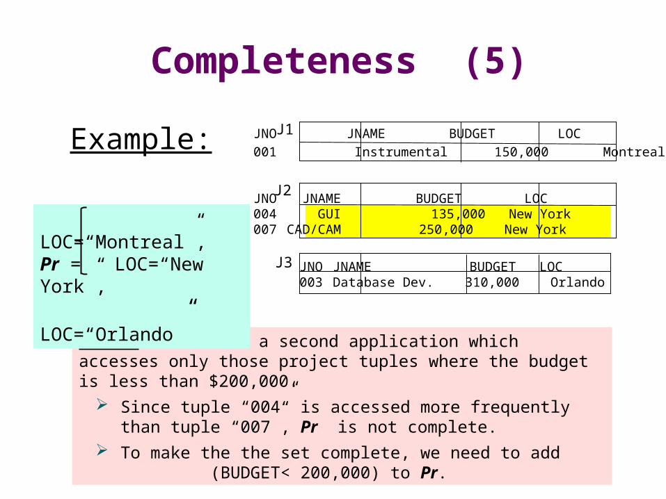
Completeness (5)
Example: JNO JNAME BUDGET LOC001 Instrumental 150,000 Montreal
JNO JNAME BUDGET LOC004 GUI 135,000 New York007 CAD/CAM 250,000 New York
J1
J2
JNO JNAME BUDGET LOC003 Database Dev. 310,000 Orlando
J3
Case 2: There is a second application which accesses only those project tuples where the budget is less than $200,000.
Since tuple “004” is accessed more frequently than tuple “007”, Pr is not complete.
To make the the set complete, we need to add (BUDGET< 200,000) to Pr.
LOC=“Montreal”,Pr = LOC=“New York”, LOC=“Orlando”
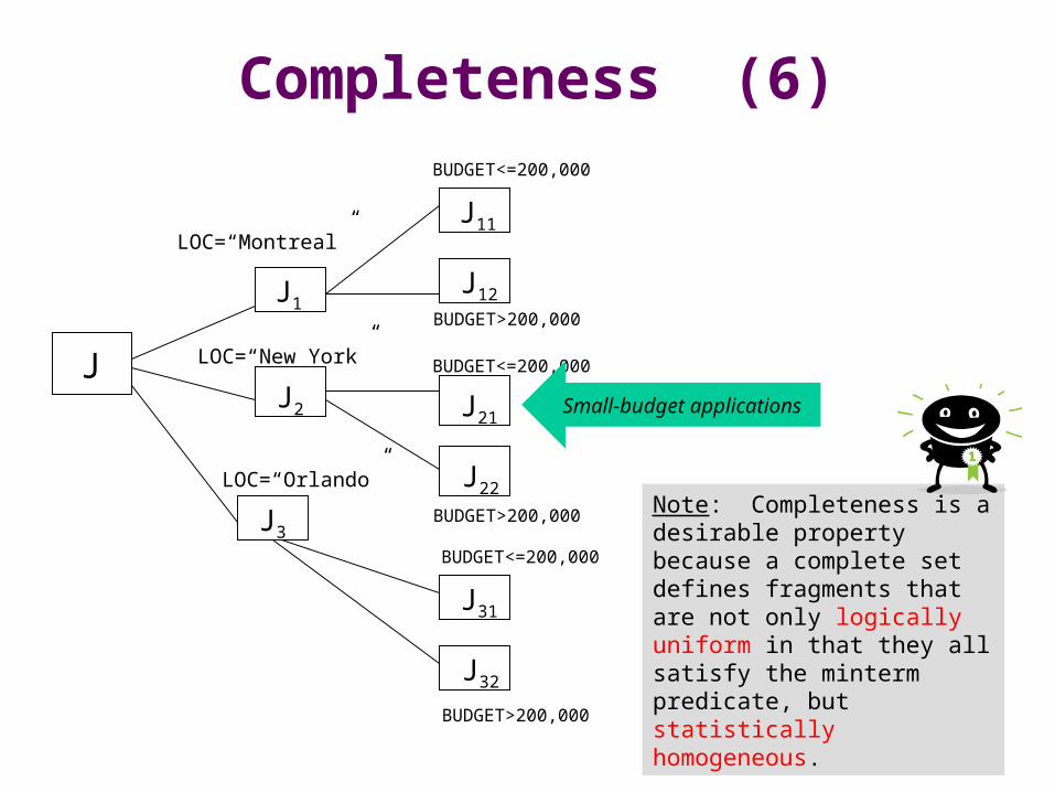
J
J1
J2
J3
LOC=“Montreal”
LOC=“New York”
LOC=“Orlando”
J11
J12
BUDGET<=200,000
BUDGET>200,000
J21
BUDGET<=200,000
J22
BUDGET>200,000
J31
J32
BUDGET>200,000
BUDGET<=200,000
Completeness (6)
Small-budget applications
Note: Completeness is a desirable property because a complete set defines fragments that are not only logically uniform in that they all satisfy the minterm predicate, but statistically homogeneous.
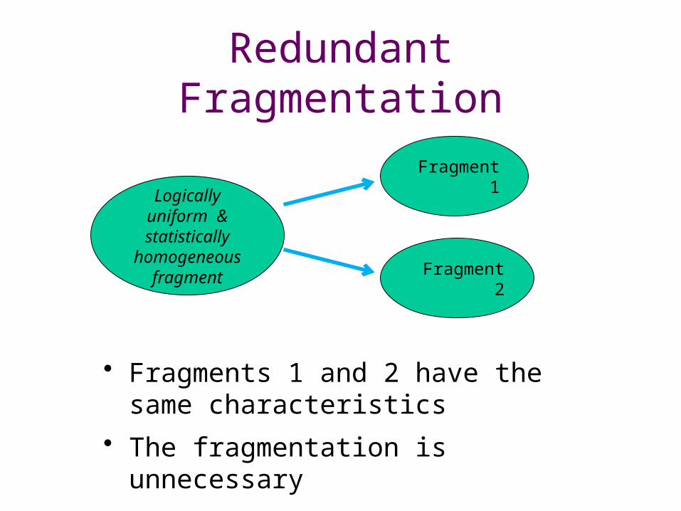
Redundant Fragmentation
• Fragments 1 and 2 have the same characteristics
• The fragmentation is unnecessary
Logically uniform & statistically
homogeneous fragment
Fragment 1
Fragment 2
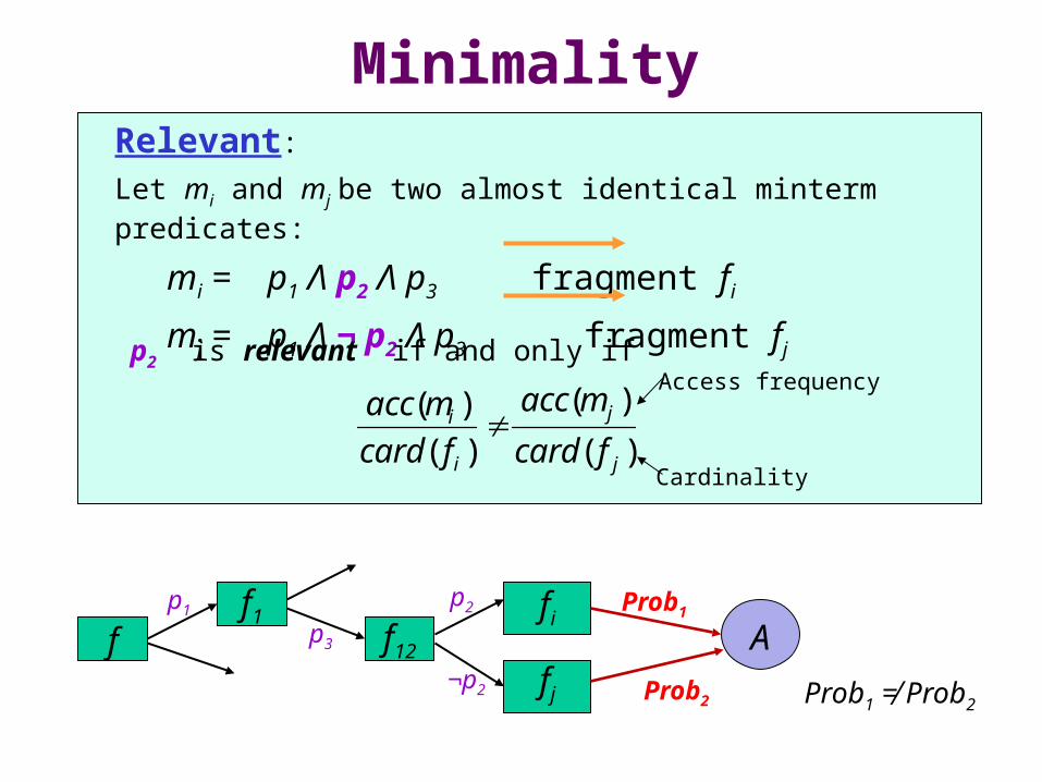
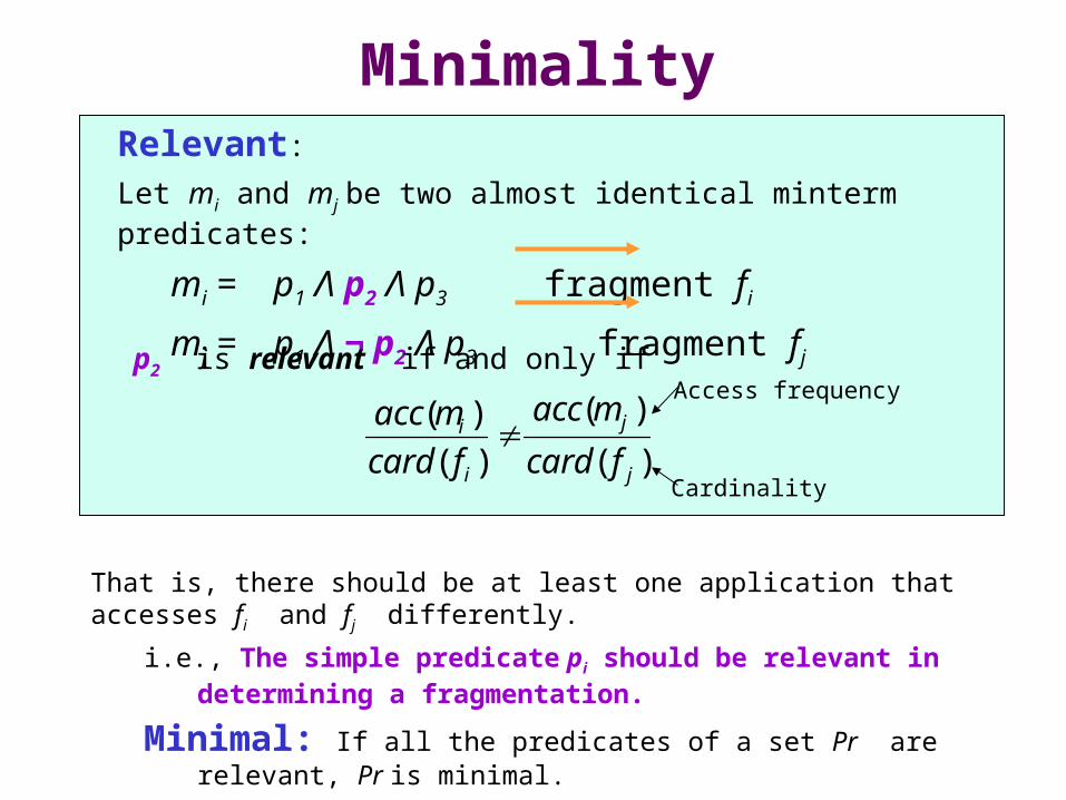
MinimalityRelevant:
Let mi and mj be two almost identical minterm predicates:
mi = p1 Λ p2 Λ p3 fragment fi
mj = p1 Λ ¬ p2 Λ p3 fragment fj
p2 is relevant if and only if
)(
)(
)(
)(
j
j
i
i
fcard
macc
fcard
macc
Access frequency
Cardinality
ff1
f12
fi
fj
p1
p3
p2
¬p2
AProb1
Prob2 Prob1 ≠ Prob2
MinimalityRelevant:
Let mi and mj be two almost identical minterm predicates:
mi = p1 Λ p2 Λ p3 fragment fi
mj = p1 Λ ¬ p2 Λ p3 fragment fj
p2 is relevant if and only if
)(
)(
)(
)(
j
j
i
i
fcard
macc
fcard
macc
Access frequency
Cardinality
That is, there should be at least one application that accesses fi and fj differently.
i.e., The simple predicate pi should be relevant in determining a fragmentation.
Minimal: If all the predicates of a set Pr are relevant, Pr is minimal.
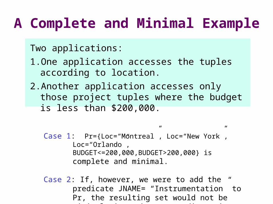
A Complete and Minimal Example
Two applications:
1. One application accesses the tuples according to location.
2. Another application accesses only those project tuples where the budget is less than $200,000.
Case 1: Pr={Loc=“Montreal”, Loc=“New York”, Loc=“Orlando”, BUDGET<=200,000,BUDGET>200,000} iscomplete and minimal.
Case 2: If, however, we were to add the predicate JNAME= “Instrumentation” to Pr, the resulting set would not be minimal since the new predicate is not relevant with respect to the applications.
J
J1
J2
J3
LOC=“Montreal”
LOC=“New York”
LOC=“Orlando”
J11
J12
BUDGET<=200,000
BUDGET>200,000
J121
J122
JNAME = “Instrument”
JNAME! “Instrument”
J21
BUDGET<=200,000
J22
BUDGET>200,000
J31
J32
RelevantBUDGET>200,000
BUDGET<=200,000
[ JNAME = “Instrument” ] is not relevant.
Irrelevant
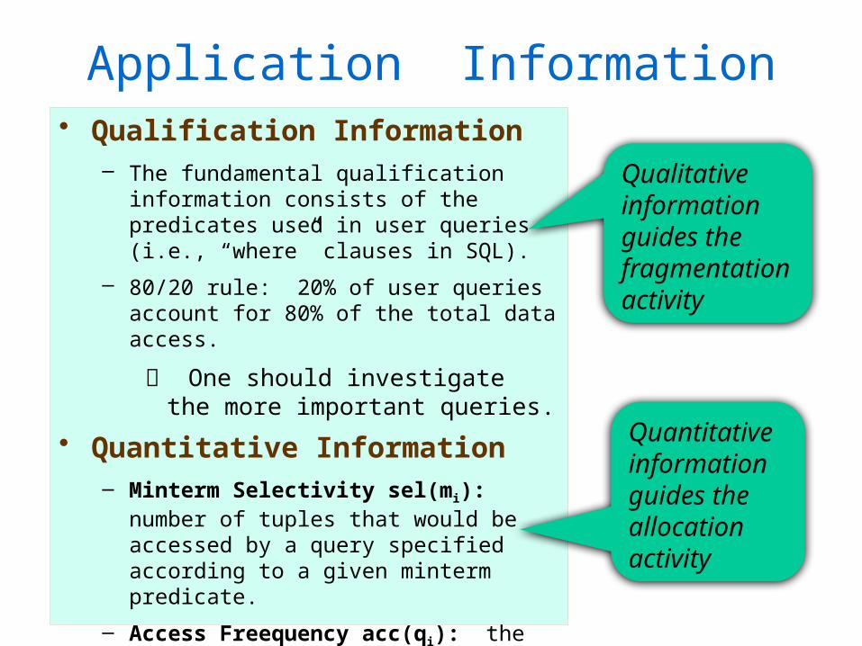
Application Information• Qualification Information
– The fundamental qualification information consists of the predicates used in user queries (i.e., “where” clauses in SQL).
– 80/20 rule: 20% of user queries account for 80% of the total data access.
One should investigate the more important queries.
• Quantitative Information– Minterm Selectivity sel(mi):
number of tuples that would be accessed by a query specified according to a given minterm predicate.
– Access Freequency acc(qi): the access frequency of queries in a given period.
Qualitative information guides the fragmentation activity
Quantitative information guides the allocation activity
Determine the set of meaningful minterm predicates
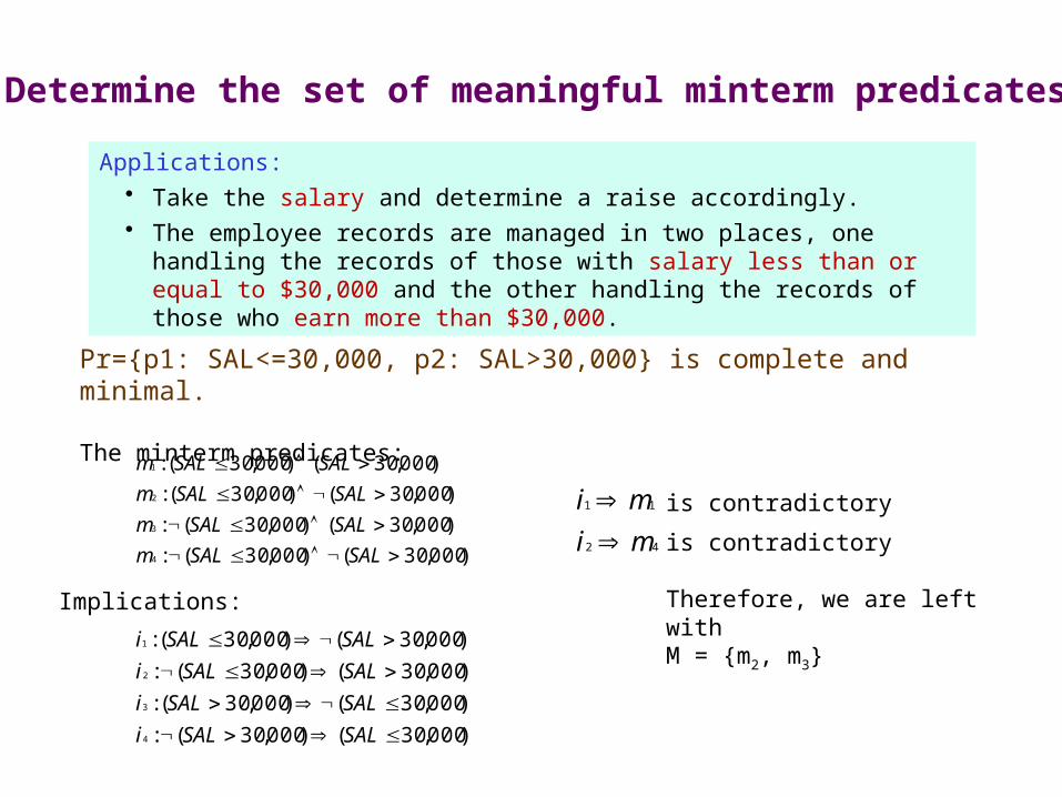
Applications: • Take the salary and determine a raise accordingly.• The employee records are managed in two places, one handling the
records of those with salary less than or equal to $30,000 and the other handling the records of those who earn more than $30,000.
)000,30()000,30(:
)000,30()000,30(:
)000,30()000,30(:
)000,30()000,30(:
4
3
2
1
SALSALm
SALSALm
SALSALm
SALSALm
Implications:
)000,30()000,30(:
)000,30()000,30(:
)000,30()000,30(:
)000,30()000,30(:
4
3
2
1
SALSALi
SALSALi
SALSALi
SALSALi
42
11
mi
mi
is contradictory
is contradictory
Therefore, we are left withM = {m2, m3}
Pr={p1: SAL<=30,000, p2: SAL>30,000} is complete and minimal.
The minterm predicates:
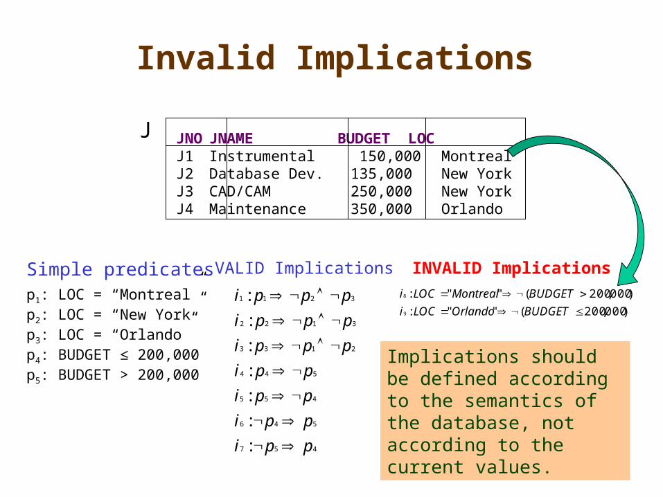
Invalid Implications
JNO JNAME BUDGET LOCJ1 Instrumental 150,000 MontrealJ2 Database Dev. 135,000 New YorkJ3 CAD/CAM 250,000 New YorkJ4 Maintenance 350,000 Orlando
J
Simple predicatesp1: LOC = “Montreal”p2: LOC = “New York”p3: LOC = “Orlando”p4: BUDGET ≤ 200,000p5: BUDGET > 200,000
VALID Implications
457
546
455
544
2133
3122
3211
:
:
:
:
:
:
:
ppi
ppi
ppi
ppi
pppi
pppi
pppi
INVALID Implications
)000,200("":
)000,200("":
9
8
BUDGETOrlandoLOCi
BUDGETMontrealLOCi
Implications should be defined according to the semantics of the database, not according to the current values.
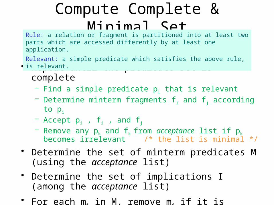
Compute Complete & Minimal Set
• Repeat until the predicate set is complete– Find a simple predicate pi that is relevant– Determine minterm fragments fi and fj according to pi
– Accept pi , fi , and fj – Remove any pk and fk from acceptance list if pk becomes
irrelevant /* the list is minimal */
• Determine the set of minterm predicates M (using the acceptance list)
• Determine the set of implications I (among the acceptance list)
• For each mi in M, remove mi if it is contradictory according to I
Rule: a relation or fragment is partitioned into at least two parts which are accessed differently by at least one application.
Relevant: a simple predicate which satisfies the above rule, is relevant.
Derived Horizontal Fragmentation
Derived fragmentation is used to facilitate the join between fragments.
In some cases, the horizontal fragmentation of a relation cannot be based on a property of its own attributes, but is derived from the horizontal fragmentation of another relation.
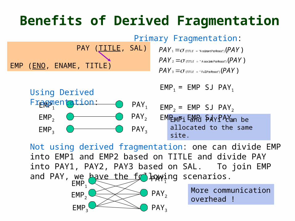
PAY (TITLE, SAL)
EMP (ENO, ENAME, TITLE)
1 ( "Assistant Professor")
2 ( " Associate Professor")
3 ( " Full Professor")
( )
( )
( )
TITLE
TITLE
TITLE
PAY PAY
PAY PAY
PAY PAY
Not using derived fragmentation: one can divide EMP into EMP1 and EMP2 based on TITLE and divide PAY into PAY1, PAY2, PAY3 based on SAL. To join EMP and PAY, we have the following scenarios.
PAY1
PAY2
PAY3
More communication overhead !
Benefits of Derived FragmentationPrimary Fragmentation:
EMP1 PAY1
EMP2PAY2 EMPi and PAYi can be
allocated to the same site.
Using Derived Fragmentation:
EMP1 = EMP SJ PAY1
EMP2 = EMP SJ PAY2
EMP3 = EMP SJ PAY3
EMP3 PAY3
EMP1
EMP2
EMP3
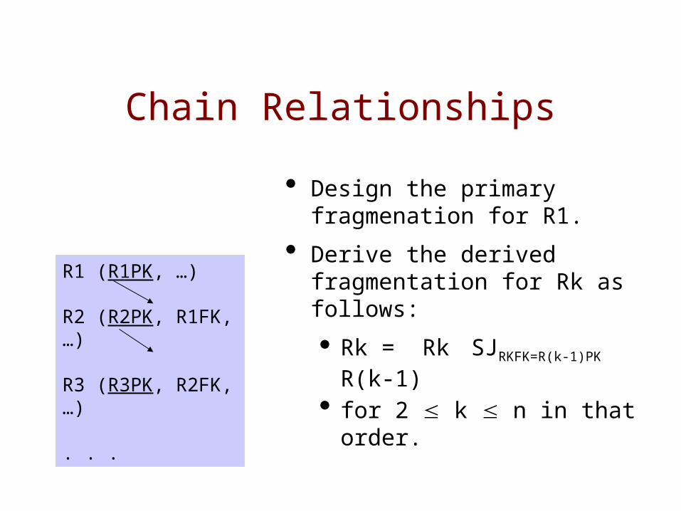
Chain Relationships
• Design the primary fragmenation for R1.
• Derive the derived fragmentation for Rk as follows:
• Rk = Rk SJRKFK=R(k-1)PK R(k-1)
• for 2 k n in that order.
R1 (R1PK, …)
R2 (R2PK, R1FK, …)
R3 (R3PK, R2FK, …)
. . .
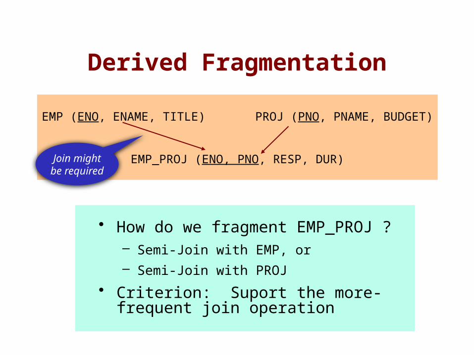
Derived Fragmentation
• How do we fragment EMP_PROJ ?– Semi-Join with EMP, or– Semi-Join with PROJ
• Criterion: Suport the more-frequent join operation
EMP (ENO, ENAME, TITLE) PROJ (PNO, PNAME, BUDGET)
EMP_PROJ (ENO, PNO, RESP, DUR)Join might
be required
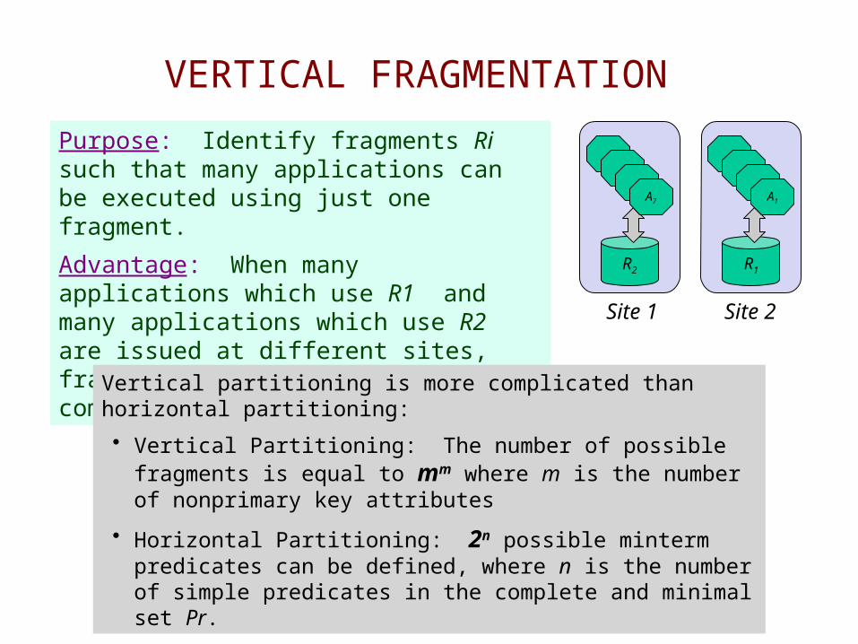
VERTICAL FRAGMENTATION
Purpose: Identify fragments Ri such that many applications can be executed using just one fragment.
Advantage: When many applications which use R1 and many applications which use R2 are issued at different sites, fragmenting R avoids communication overhead.
Vertical partitioning is more complicated than horizontal partitioning:
• Vertical Partitioning: The number of possible fragments is equal to mm where m is the number of nonprimary key attributes
• Horizontal Partitioning: 2n possible minterm predicates can be defined, where n is the number of simple predicates in the complete and minimal set Pr.
R1R2
A1A7
Site 1 Site 2
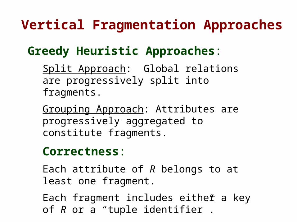
Greedy Heuristic Approaches:
Split Approach: Global relations are progressively split into fragments.
Grouping Approach: Attributes are progressively aggregated to constitute fragments.
Correctness:
Each attribute of R belongs to at least one fragment.
Each fragment includes either a key of R or a “tuple identifier”.
Vertical Fragmentation Approaches
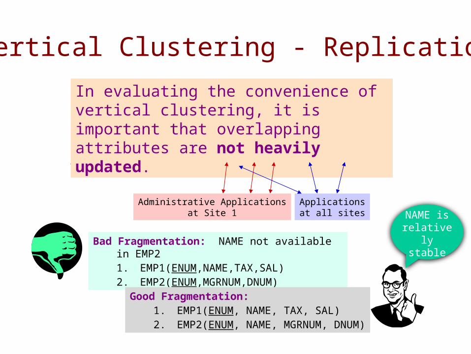
Vertical Clustering - Replication
Example: EMP(ENUM,NAME,SAL,TAX,MGRNUM,DNUM)
Bad Fragmentation: NAME not available in EMP21. EMP1(ENUM,NAME,TAX,SAL)2. EMP2(ENUM,MGRNUM,DNUM)
Good Fragmentation: 1. EMP1(ENUM, NAME, TAX, SAL)2. EMP2(ENUM, NAME, MGRNUM, DNUM)
In evaluating the convenience of vertical clustering, it is important that overlapping attributes are not heavily updated.
Administrative Applicationsat Site 1
Applicationsat all sites
NAME is relatively
stable
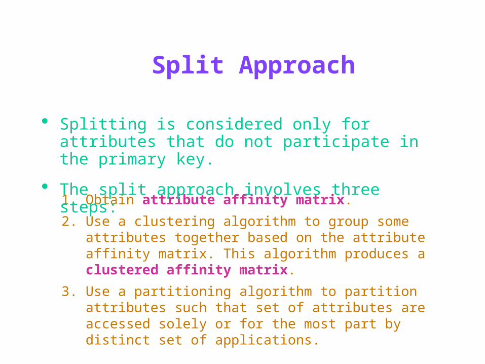
Split Approach
1. Obtain attribute affinity matrix.
2. Use a clustering algorithm to group some attributes together based on the attribute affinity matrix. This algorithm produces a clustered affinity matrix.
3. Use a partitioning algorithm to partition attributes such that set of attributes are accessed solely or for the most part by distinct set of applications.
• Splitting is considered only for attributes that do not participate in the primary key.
• The split approach involves three steps:
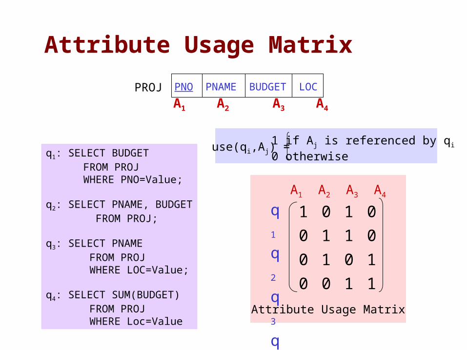
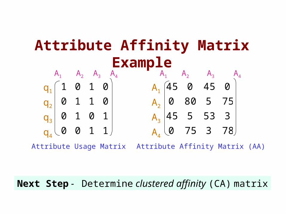
PNO PNAME BUDGET LOCPROJA1 A2 A3 A4
q1: SELECT BUDGET FROM PROJ WHERE PNO=Value;
q2: SELECT PNAME, BUDGET FROM PROJ;
q3: SELECT PNAME FROM PROJ WHERE LOC=Value;
q4: SELECT SUM(BUDGET) FROM PROJ WHERE Loc=Value
1100
1010
0110
0101
A1 A2 A3 A4
q1
q2
q3
q4
Attribute Usage Matrix
1 if Aj is referenced by qi
0 otherwise
Attribute Usage Matrix
use(qi,Aj) =
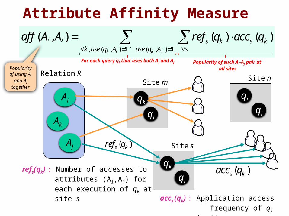
Attribute Affinity Measure
Ai
Ak
Aj
Relation RSite m
qk
qi
Site s
qk
qi
Site n
qi
qi
( )s kref q
( )s kacc qrefs(qk) : Number of accesses to attributes (Ai,Aj) for each execution of qk at site s
accs (qk) : Application access frequency of qk at site s.
, ( , ) 1 ( , ) 1
( , ) ( ) ( )i j
k i k j
s k s kk use q A use q A s
aff A A ref q acc q
For each query qk that uses both Ai and Aj Popularity of such Ai-Aj pair at
all sitesPopularity of
using Ai and Aj
together
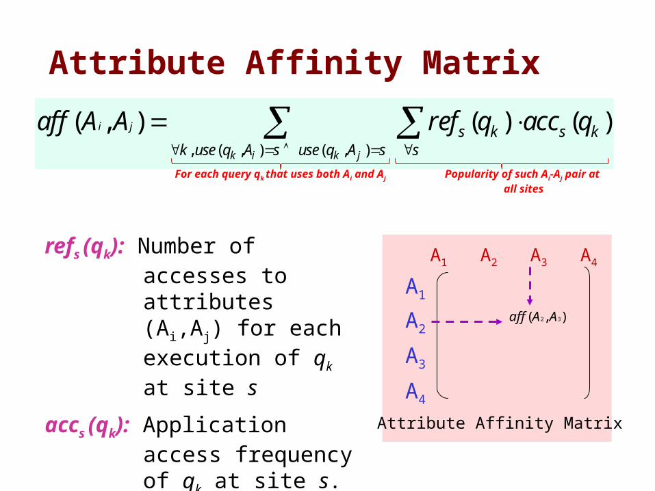
A1 A2 A3 A4
A1
A2
A3
A4
Attribute Affinity Matrix
Attribute Affinity Matrix
),( 32 AAaff
refs (qk): Number of accesses to attributes (Ai,Aj) for each execution of qk at site s
accs (qk): Application access frequency of qk at site s.
, ( , ) ( , )
( , ) ( ) ( )i j
k i k j
s k s kk use q A s use q A s s
aff A A ref q acc q
For each query qk that uses both Ai and Aj Popularity of such Ai-Aj pair at
all sites
1100
1010
0110
0101
A1 A2 A3 A4
q1
q2
q3
q4
Attribute Usage Matrix
783750
353545
755800
045045
A1 A2 A3 A4
A1
A2
A3
A4
Attribute Affinity Matrix (AA)
Attribute Affinity Matrix Example
Next Step - Determine clustered affinity (CA) matrix
783750
353545
755800
045045
A1 A2 A3 A4
A1
A2
A3
A4
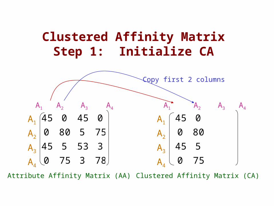
Attribute Affinity Matrix (AA)
Clustered Affinity MatrixStep 1: Initialize CA
750
545
800
045
A1 A2 A3 A4
A1
A2
A3
A4
Clustered Affinity Matrix (CA)
Copy first 2 columns
783750
353545
755800
045045
A1 A2 A3 A4
A1
A2
A3
A4
Attribute Affinity Matrix (AA)
Clustered Affinity MatrixStep 2: Determine Location for A3
750
545
800
045
A1 A2
A1
A2
A3
A4
Clustered Affinity Matrix (CA)
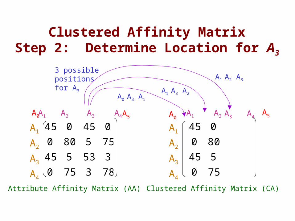
3 possiblepositionsfor A3
A0 A0A5
A5A3 A4
A1 A2 A3
A1 A3 A2A0 A3 A1
Clustered Affinity MatrixStep 2: Determine the order for A3
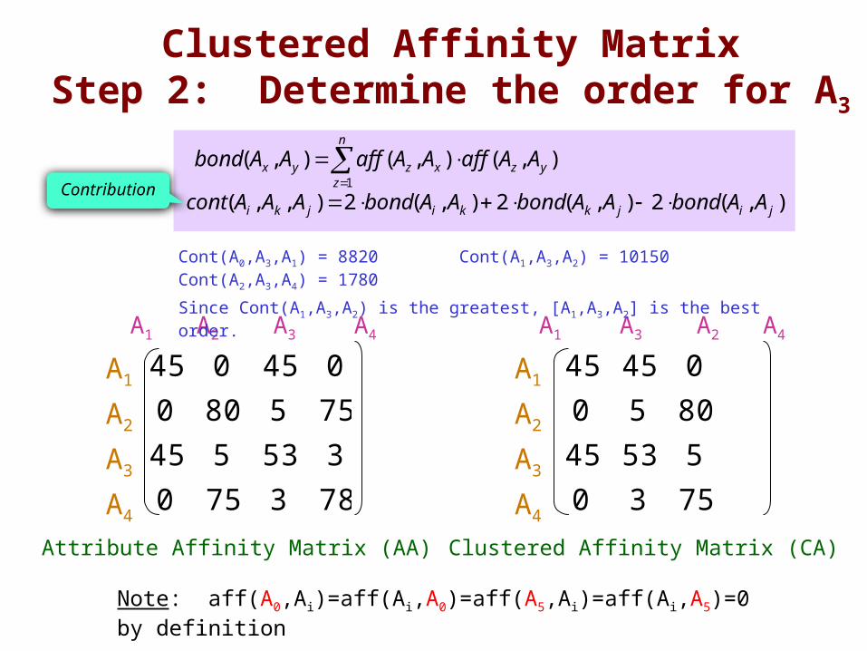
n
zyzxzyx AAaffAAaffAAbond
1
),(),(),(
),(2),(2),(2),,( jijkkijki AAbondAAbondAAbondAAAcont
783750
353545
755800
045045
A1 A2 A3 A4
A1
A2
A3
A4
Attribute Affinity Matrix (AA)
7530
55345
8050
04545
A1 A3 A2 A4
A1
A2
A3
A4
Clustered Affinity Matrix (CA)
Cont(A0,A3,A1) = 8820 Cont(A1,A3,A2) = 10150 Cont(A2,A3,A4) = 1780
Since Cont(A1,A3,A2) is the greatest, [A1,A3,A2] is the best order.
Note: aff(A0,Ai)=aff(Ai,A0)=aff(A5,Ai)=aff(Ai,A5)=0 by definition
Contribution
783750
353545
755800
045045
A1 A2 A3 A4
A1
A2
A3
A4
Attribute Affinity Matrix (AA)
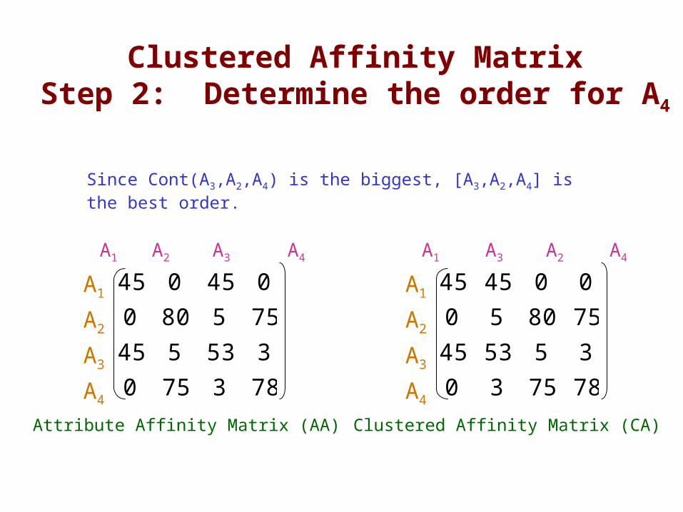
Clustered Affinity MatrixStep 2: Determine the order for A4
787530
355345
758050
004545
A1 A3 A2 A4
A1
A2
A3
A4
Clustered Affinity Matrix (CA)
Since Cont(A3,A2,A4) is the biggest, [A3,A2,A4] is the best order.
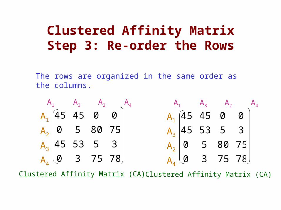
Clustered Affinity MatrixStep 3: Re-order the Rows
787530
758050
355345
004545
A1 A3 A2 A4
A1
A3
A2
A4
Clustered Affinity Matrix (CA)
The rows are organized in the same order as the columns.
787530
355345
758050
004545
A1 A3 A2 A4
A1
A2
A3
A4
Clustered Affinity Matrix (CA)
787530
758050
355345
004545
A1 A3 A2 A4
A1
A3
A2
A4
Clustered Affinity Matrix (CA)
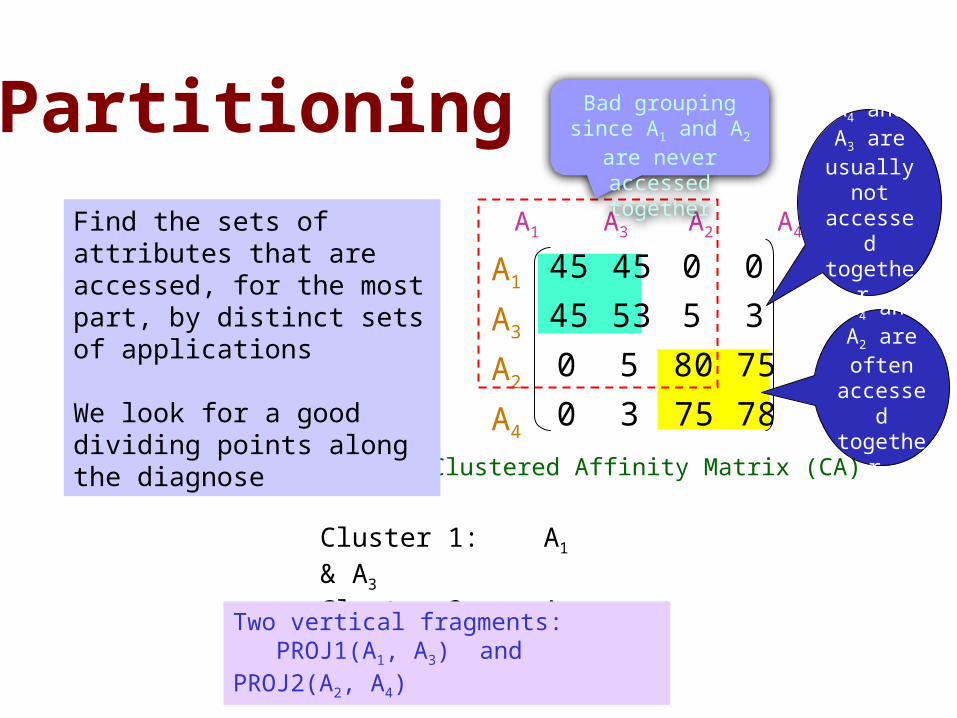
PartitioningFind the sets of attributes that are accessed, for the most part, by distinct sets of applications
We look for a good dividing points along the diagnose
Cluster 1: A1 & A3
Cluster 2: A2 & A4
Two vertical fragments: PROJ1(A1, A3) and PROJ2(A2, A4)
A4 and A3 are
usually not
accessed together
A4 and A2 are often
accessed
together
Bad grouping since A1 and A2 are never accessed together
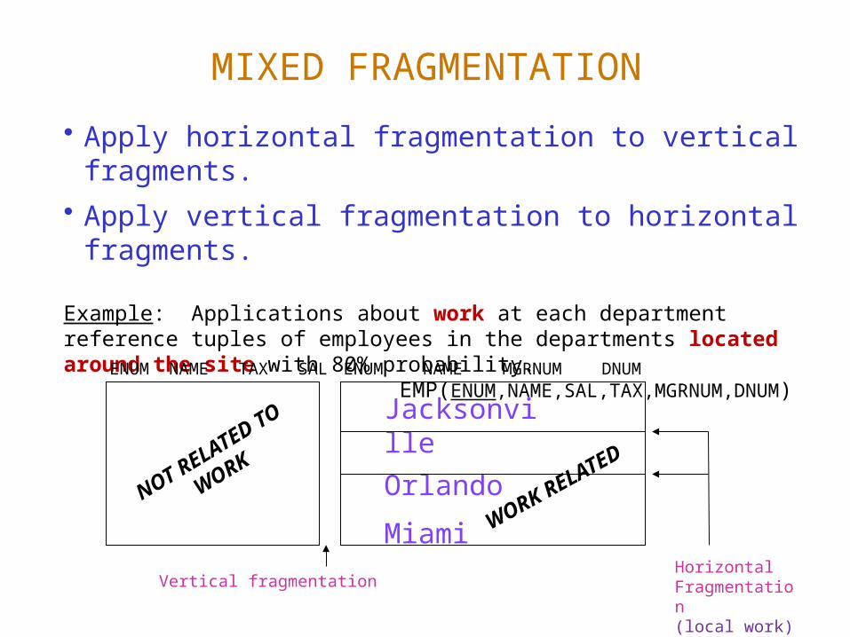
MIXED FRAGMENTATION
• Apply horizontal fragmentation to vertical fragments.
• Apply vertical fragmentation to horizontal fragments.
Example: Applications about work at each department reference tuples of employees in the departments located around the site with 80% probability.
EMP(ENUM,NAME,SAL,TAX,MGRNUM,DNUM)ENUM NAME TAX SAL ENUM NAME MGRNUM DNUM
Jacksonville
Orlando
Miami
Vertical fragmentationHorizontal Fragmentation(local work)
NOT RELATED TO
WORK
WORK RELATED
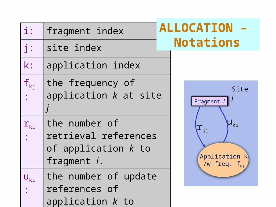
i: fragment index
j: site index
k: application index
fkj: the frequency of application k at site j
rki: the number of retrieval references of application k to fragment i.
uki: the number of update references of application k to fragment i.
nki =
rki + uki
ALLOCATION – Notations
Fragment i
Application k/w freq. fkj
rki
uki
Site j
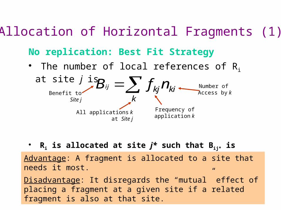
Allocation of Horizontal Fragments (1)
No replication: Best Fit Strategy
• The number of local references of Ri at site j is
• Ri is allocated at site j* such that Bij* is
maximum.
k
kikjnfBij
Advantage: A fragment is allocated to a site that needs it most.
Disadvantage: It disregards the “mutual” effect of placing a fragment at a given site if a related fragment is also at that site.
All applications kat Site j
Frequency ofapplication k
Number of Access by kBenefit to
Site j
Allocation of Horizontal Fragments (2)
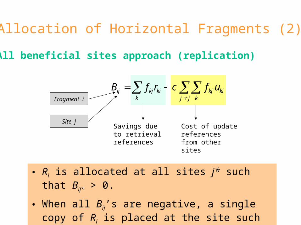
All beneficial sites approach (replication)
k jj k
kikjkikjij ufcrfB'
'
Savings due to retrieval references
Cost of update references from other sites
• Ri is allocated at all sites j* such that Bij* > 0.
• When all Bij’s are negative, a single copy of Ri is placed at the site such that Bij* is maximum.
Fragment i
Site j

Allocation of Horizontal Fragments (3)
Another Replication Approach:
di The degree of redundancy of Ri
Fi
The reliability and availability benefit of having Ri fully replicated.
(di)The reliability and availability benefit when the fragment has di copies.
,4
3)3(,2
)2(,0)1()21()( 1 FFFd
iii
di
i
The benefit of introducing a new copy of Ri at site j :
)('
' dufcrfB ik k jj
kikjkikjij
Same as All BeneficialSites approach
Also takes into account the benefit of availability
β
1
Fi
di
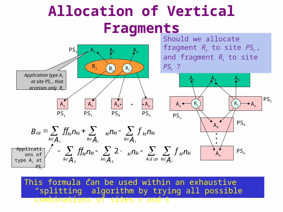
Allocation of Vertical Fragments
This formula can be used within an exhaustive “splitting” algorithm by trying all possible combinations of sites s and t.
1
2 34
2
s t
l
ist ks kt ksks kt ksk k k
kt ki kikt ki kll nk k k
f f fn n nBA A A
f f fn n nA A A
Applications of type As
at PSs
As At A4 An
PSr A1 A3 A2
Ri RsRt
PSs PSt PS4 PSn
. . .
Application type A1 at site PSr , that
accesses only Rs
Rs RtAs At
A1 A3 A2
PSr
PSs
PSt
PS4
PSn
A4
An
...
Should we allocate fragment Rs to site PSs , and fragment Rt to site PSt ?
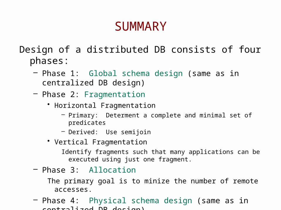
SUMMARY
Design of a distributed DB consists of four phases:– Phase 1: Global schema design (same as in centralized
DB design)– Phase 2: Fragmentation
• Horizontal Fragmentation– Primary: Determent a complete and minimal set of
predicates– Derived: Use semijoin
• Vertical FragmentationIdentify fragments such that many applications can be
executed using just one fragment.
– Phase 3: AllocationThe primary goal is to minize the number of remote
accesses.
– Phase 4: Physical schema design (same as in centralized DB design).
Database IntegrationBottom-up Design
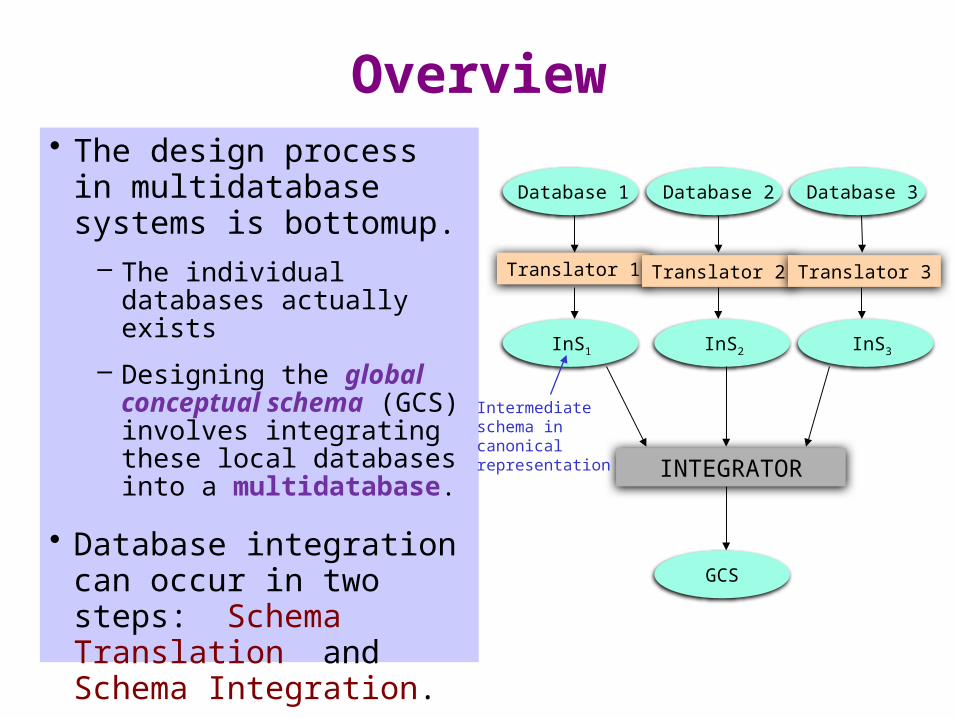
Overview• The design process in
multidatabase systems is bottomup.
– The individual databases actually exists
– Designing the global conceptual schema (GCS) involves integrating these local databases into a multidatabase.
• Database integration can occur in two steps: Schema Translation and Schema Integration.
Database 1 Database 2 Database 3
Translator 1 Translator 2 Translator 3
InS1
INTEGRATOR
GCS
Intermediate schema in canonicalrepresentation
InS3InS2
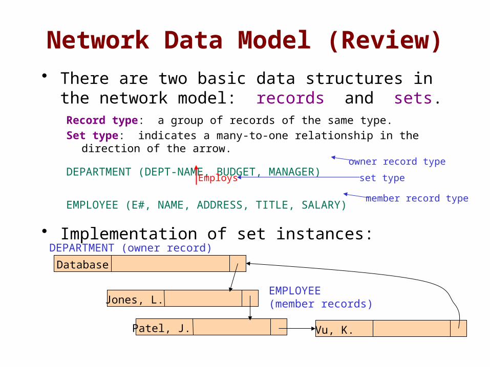
Network Data Model (Review)
• There are two basic data structures in the network model: records and sets.Record type: a group of records of the same type.Set type: indicates a many-to-one relationship in the direction of the
arrow.
DEPARTMENT (DEPT-NAME, BUDGET, MANAGER)
EMPLOYEE (E#, NAME, ADDRESS, TITLE, SALARY)
• Implementation of set instances:
Employs
owner record type
set type
member record type
Database
Jones, L.
Patel, J. Vu, K.
DEPARTMENT (owner record)
EMPLOYEE(member records)
Example: Three Local Databases
Database 1 (Relational Model):
S (TITLE, SAL)
E (ENO, ENAME, TITLE) J (JNO, JNAME, BUDGET, LOC, CNAME)
G (ENO, JNO, RESP, DUR)
Database 2 (Network Model):DEPARTMENT (DEPT_NAME, BUDGET, MANAGER)
Work
EMPLOYEE (E#, NAME, ADDRESS, TITLE, SALARY)
Employs
Worksin
Dummy Record Type
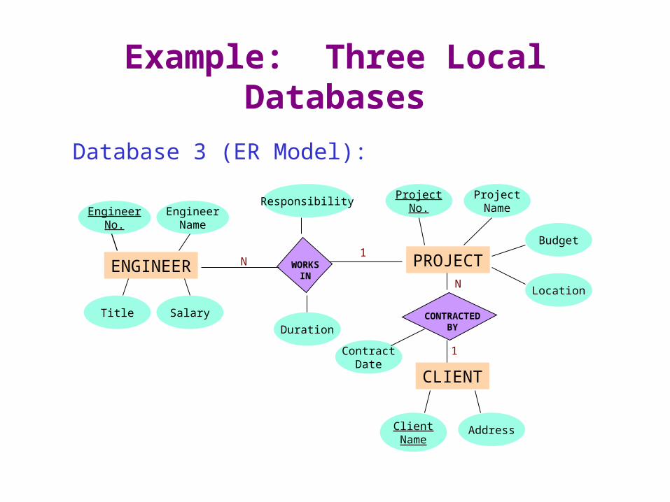
Example: Three Local Databases
Database 3 (ER Model):
EngineerNo.
EngineerName
Title Salary
ProjectNo.
ProjectName
Budget
Location
Duration
Responsibility
ContractDate
AddressClientName
ENGINEER WORKSIN
PROJECT
CONTRACTEDBY
CLIENT
1N
N
1
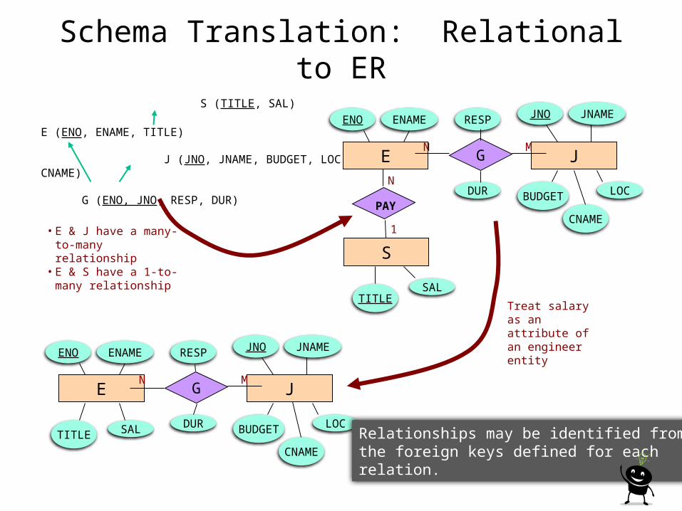
Schema Translation: Relational to ER
S (TITLE, SAL)
E (ENO, ENAME, TITLE) J (JNO, JNAME, BUDGET, LOC, CNAME)
G (ENO, JNO, RESP, DUR)
ENO ENAME
TITLESAL
E
PAY
S
G
CNAME
LOC
J
BUDGET
JNO JNAME
DUR
RESP
N M
1
N
ENO ENAME
TITLE SAL
E G
CNAME
LOC
J
BUDGET
JNO JNAME
DUR
RESP
N M
• E & J have a many-to-many relationship
• E & S have a 1-to-many relationship
Treat salary as an attribute of an engineer entity
Relationships may be identified fromthe foreign keys defined for eachrelation.
Schema Translation: Network to ER
• Map each record type in the network schema to an entity and each set type to a relationship.
• Network model uses dummy records in its representation of many-to-many relationships that need to be recognized during mapping.
DEPARTMENT EMPLOYEE
WORK
Employs Works-in
WORK
DEPARTMENT EMPLOYEE
EMPLOYS WORKS-IN
N M
11
DEPARTMENT EMPLOYS EMPLOYEEN M
Dummy record type
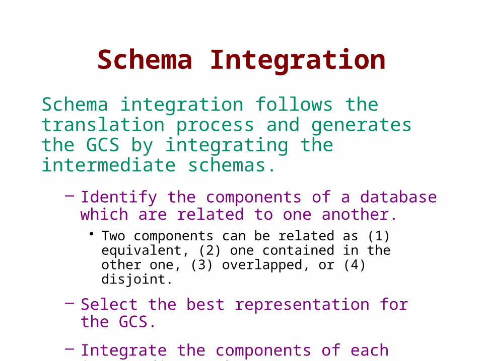
Schema Integration
Schema integration follows the translation process and generates the GCS by integrating the intermediate schemas.
– Identify the components of a database which are related to one another.• Two components can be related as (1) equivalent,
(2) one contained in the other one, (3) overlapped, or (4) disjoint.
– Select the best representation for the GCS.
– Integrate the components of each intermediate schema.
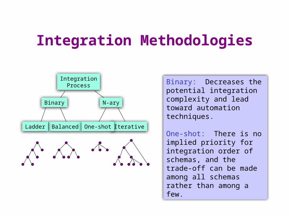
Integration Methodologies
IntegrationProcess
N-aryBinary
BalancedLadder IterativeOne-shot
Binary: Decreases the potential integration complexity and lead toward automation techniques.
One-shot: There is no implied priority for integration order of schemas, and the trade-off can be made among all schemas rather than among a few.
Integration Process
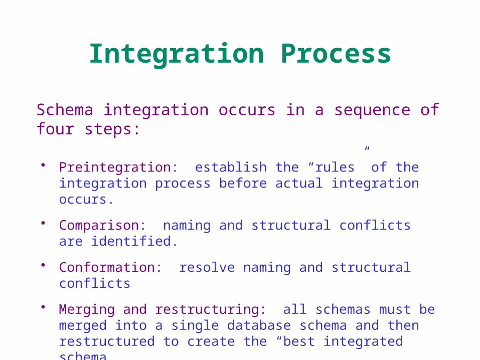
• Preintegration: establish the “rules” of the integration process before actual integration occurs.
• Comparison: naming and structural conflicts are identified.
• Conformation: resolve naming and structural conflicts
• Merging and restructuring: all schemas must be merged into a single database schema and then restructured to create the “best integrated schema.
Schema integration occurs in a sequence of four steps:
Schema Integration: Preintegration
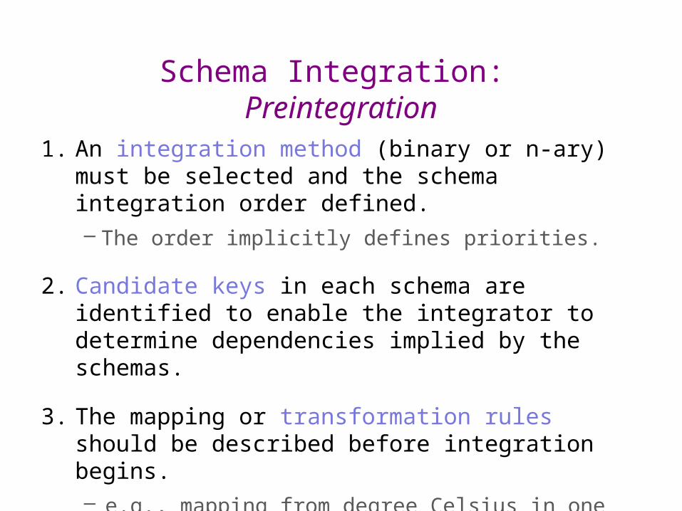
1. An integration method (binary or n-ary) must be selected and the schema integration order defined.– The order implicitly defines priorities.
2. Candidate keys in each schema are identified to enable the integrator to determine dependencies implied by the schemas.
3. The mapping or transformation rules should be described before integration begins.– e.g., mapping from degree Celsius in one schema
to degrees Fahrenheit in another.
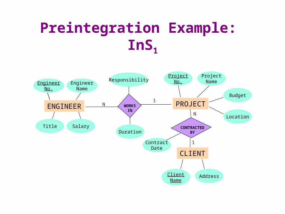
Preintegration Example: InS1
EngineerNo.
EngineerName
Title Salary
ProjectNo.
ProjectName
Budget
Location
Duration
Responsibility
ContractDate
AddressClientName
ENGINEER WORKSIN
PROJECT
CONTRACTEDBY
CLIENT
1N
N
1
Preintegration Example: InS2 & InS3
E#
Name
Address Salary
Dept-name Budget
Manager
EMPLOYEE DEPARTMENTEMPLOYS1N
InS2
Eno Ename
Title Sal
JNO Jname
Budget
LocDur
Resp
Cname
ENGINEER J MN EMPLOYS
InS3
Title
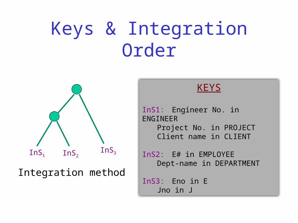
Keys & Integration Order
InS1 InS2InS3
KEYS
InS1: Engineer No. in ENGINEERProject No. in PROJECTClient name in CLIENT
InS2: E# in EMPLOYEEDept-name in DEPARTMENT
InS3: Eno in EJno in J
Integration method
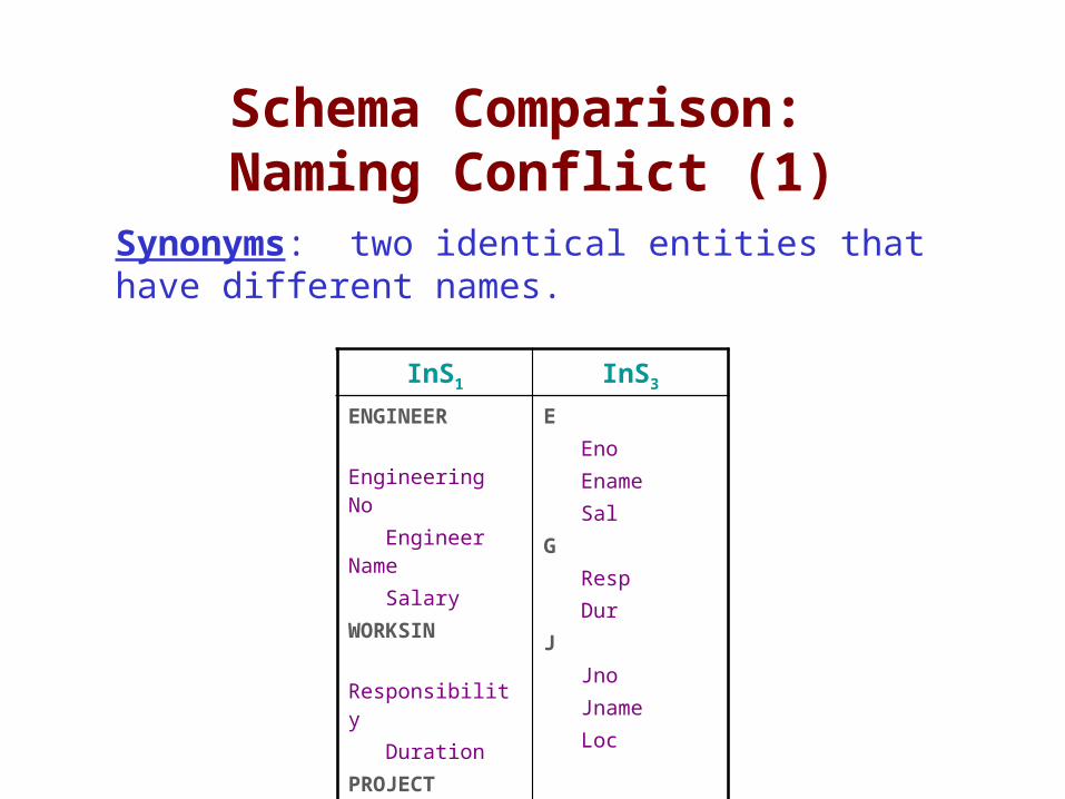
Schema Comparison: Naming Conflict (1)
Synonyms: two identical entities that have different names.
InS1 InS3
ENGINEER Engineering No Engineer Name SalaryWORKSIN Responsibility DurationPROJECT Project No Project Name Location
E Eno Ename SalG Resp DurJ Jno Jname Loc
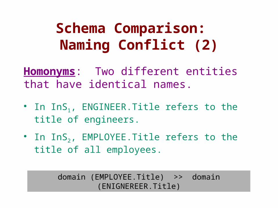
Schema Comparison: Naming Conflict (2)
• In InS1, ENGINEER.Title refers to the title of engineers.
• In InS2, EMPLOYEE.Title refers to the title of all employees.
Homonyms: Two different entities that have identical names.
domain (EMPLOYEE.Title) >> domain (ENIGNEREER.Title)
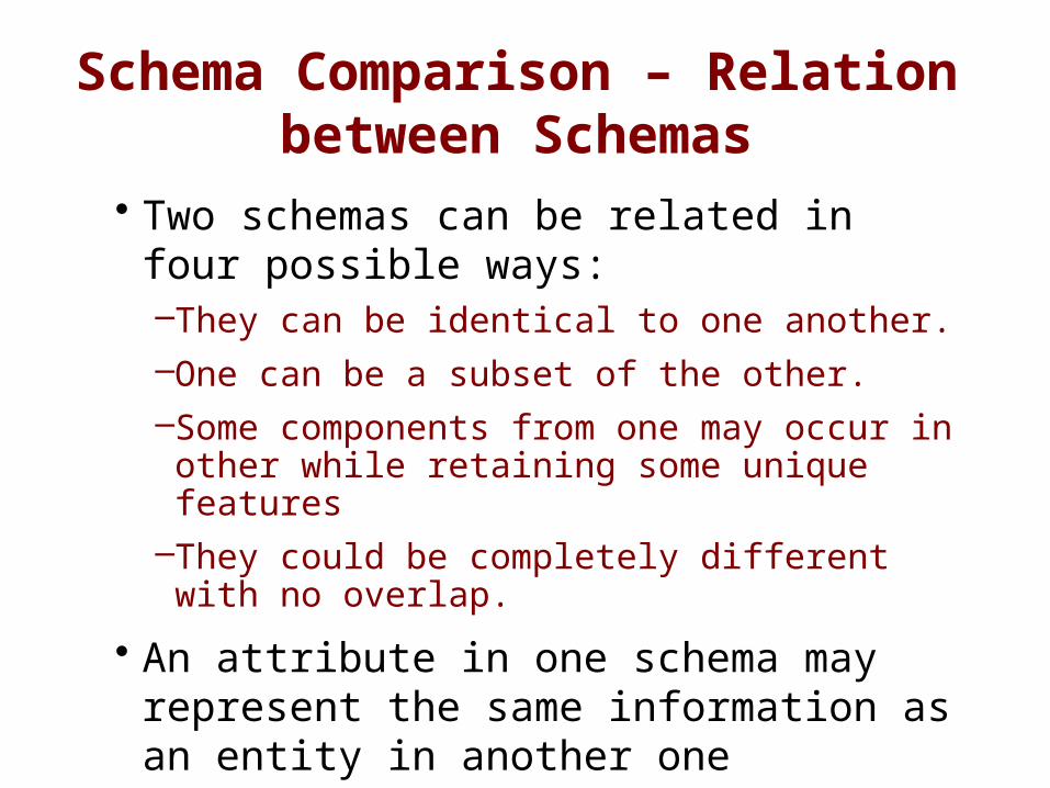
Schema Comparison – Relation between Schemas• Two schemas can be related in four
possible ways:–They can be identical to one another.–One can be a subset of the other.–Some components from one may occur in other while retaining some unique features
–They could be completely different with no overlap.
• An attribute in one schema may represent the same information as an entity in another one
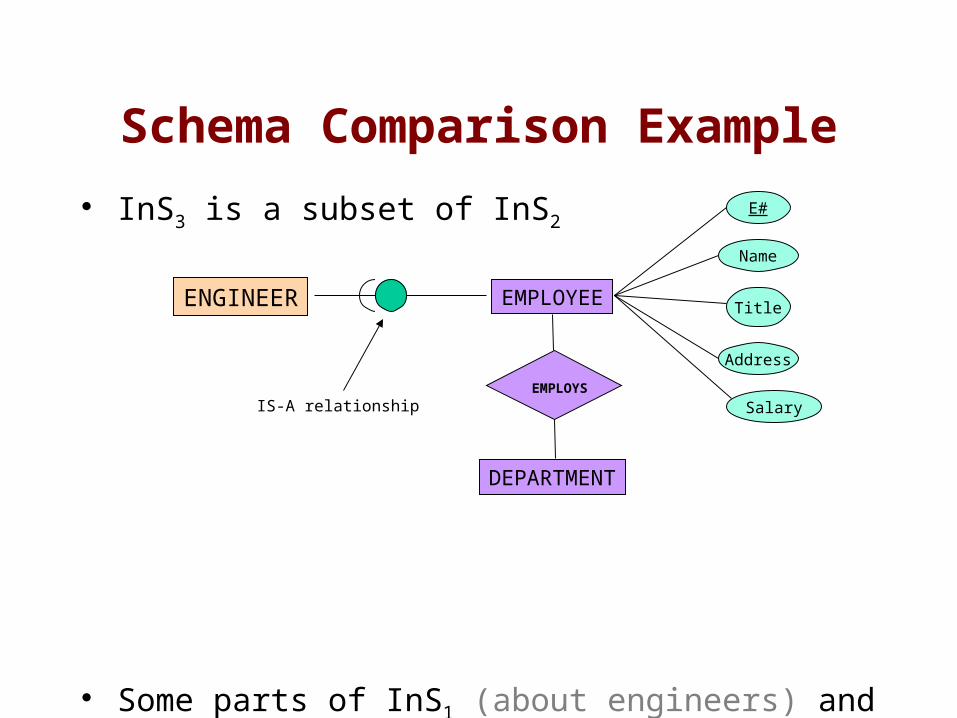
Schema Comparison Example
• InS3 is a subset of InS2
• Some parts of InS1 (about engineers) and InS3 (about engineers) occur in InS2 (about employees)
ENGINEER
EMPLOYS
E#
Name
Title
Salary
Address
IS-A relationship
DEPARTMENT
EMPLOYEE
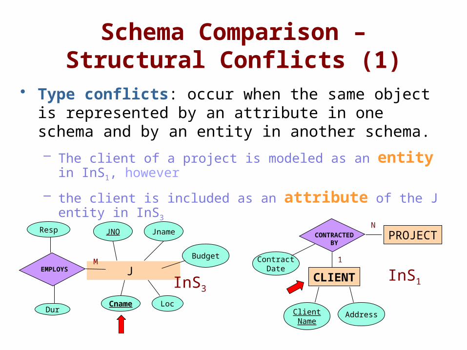
Schema Comparison – Structural Conflicts (1)
• Type conflicts: occur when the same object is represented by an attribute in one schema and by an entity in another schema.
– The client of a project is modeled as an entity in InS1, however
– the client is included as an attribute of the J entity in InS3
JNO Jname
Budget
LocDur
Resp
Cname
J M
EMPLOYS
InS3
ContractDate
AddressClientName
PROJECTCONTRACTEDBY
CLIENT
N
1
InS1
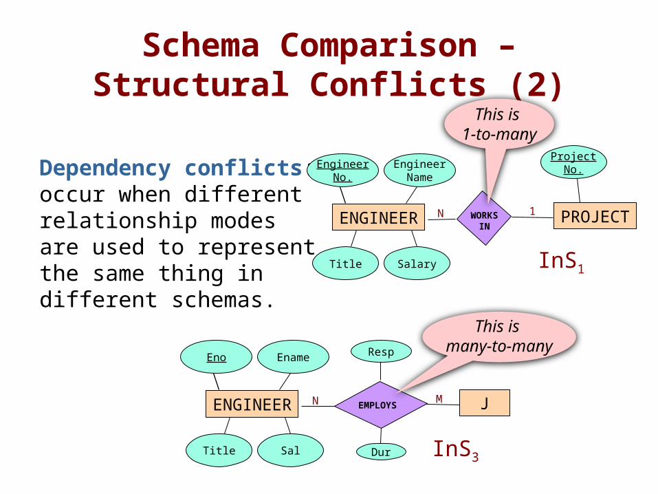
Schema Comparison – Structural Conflicts (2)
Dependency conflicts: occur when different relationship modes are used to represent the same thing in different schemas.
EngineerNo.
EngineerName
Title Salary
ProjectNo.
ENGINEER WORKSIN
PROJECT1N
InS1
Eno Ename
Title Sal Dur
Resp
ENGINEER JMN EMPLOYS
InS3
This is 1-to-many
This is many-to-
many
Schema Comparison: Structural Conflicts (3)
• Key conflicts: occur when different candidate keys are available and different primary keys are selected in different schemas
• Behavioral conflicts: are implied by the modeling mechanism,
– e.g., deletion of the last employee causes the dissolution of the department.
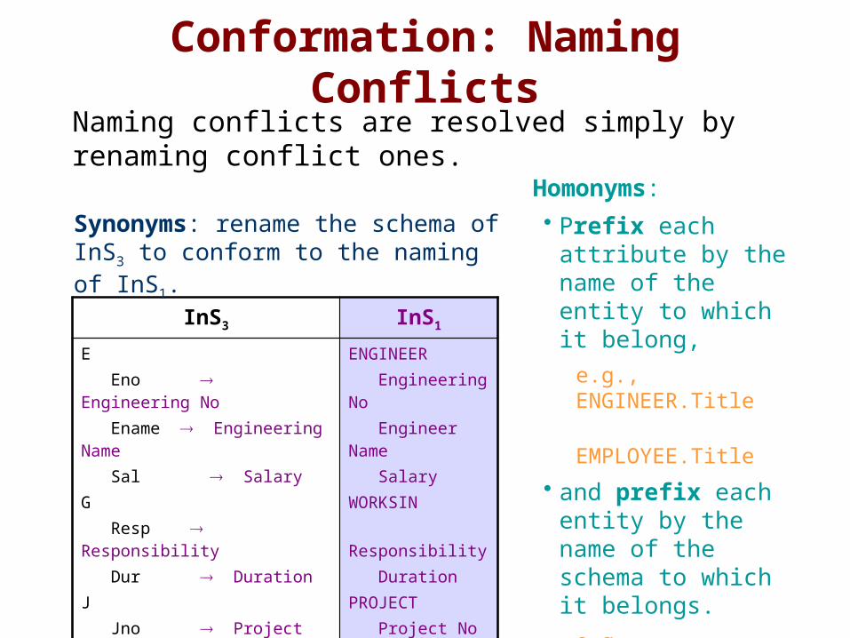
Conformation: Naming Conflicts
Naming conflicts are resolved simply by renaming conflict ones.
InS3 InS1
E Eno Engineering No Ename Engineering Name Sal SalaryG Resp Responsibility Dur DurationJ Jno Project No Jname Project Name Loc Location
ENGINEER Engineering No Engineer Name SalaryWORKSIN Responsibility DurationPROJECT Project No Project Name Location
Homonyms: • Prefix each
attribute by the name of the entity to which it belong,
e.g., ENGINEER.Title EMPLOYEE.Title
• and prefix each entity by the name of the schema to which it belongs.
e.g., InS1.ENGINEER InS2.EMPLOYEE
Synonyms: rename the schema of InS3 to conform to the naming of InS1.
EngineerNo.
EngineerName
Title Salary
Budget
Location
Duration
Responsibility
ENGINEER WORKSIN
PROJECT
ClientName
N
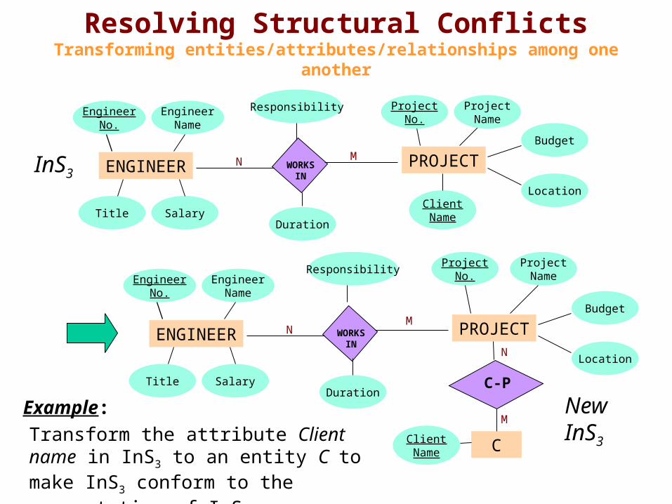
Resolving Structural ConflictsTransforming entities/attributes/relationships among one another
Transform the attribute Client name in InS3 to an entity C to make InS3 conform to the presentation of InS1.
M
EngineerNo.
EngineerName
Title Salary
ProjectNo.
ProjectName
Budget
Location
Duration
Responsibility
ENGINEER WORKSIN
PROJECTM
N
Example:
ProjectNo.
ProjectName
C-P
C
N
M
ClientName
InS3
NewInS3
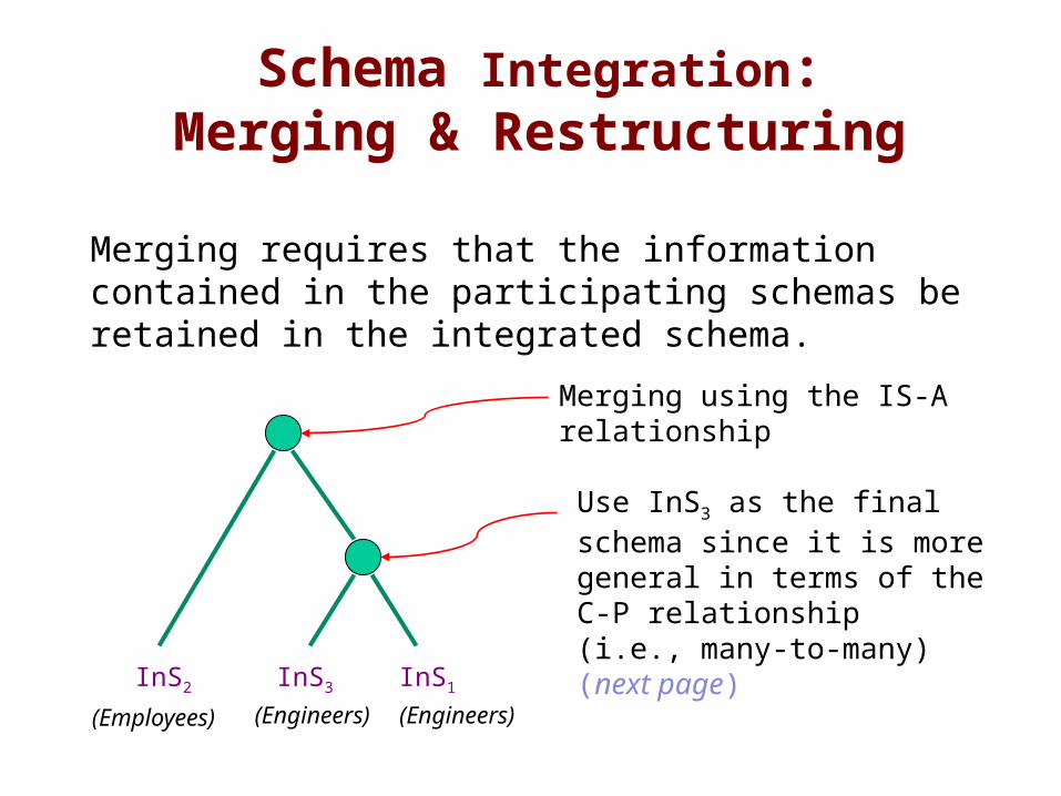
Schema Integration:Merging & Restructuring
Merging requires that the information contained in the participating schemas be retained in the integrated schema.
InS1InS2 InS3
Merging using the IS-A relationship
Use InS3 as the final schema since it is more general in terms of the C-P relationship(i.e., many-to-many) (next page)
(Employees) (Engineers) (Engineers)
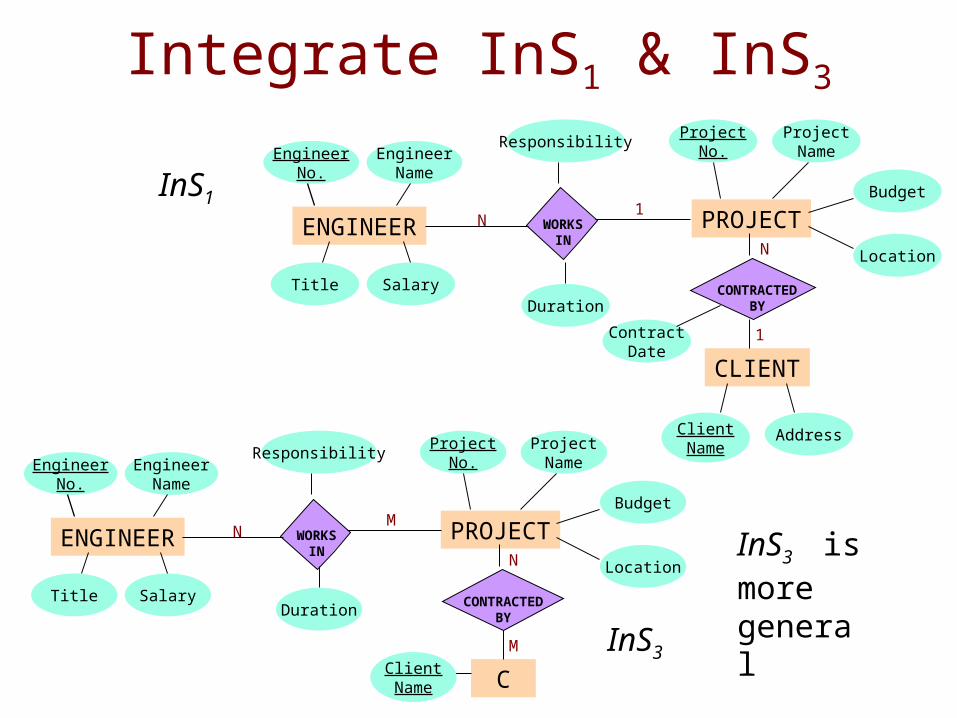
Integrate InS1 & InS3
EngineerNo.
EngineerName
Title Salary
ProjectNo.
ProjectName
Budget
Location
Duration
Responsibility
ENGINEER WORKSIN
PROJECT
CONTRACTEDBY
C
MN
N
MClientName
EngineerNo.
EngineerName
Title Salary
ProjectNo.
ProjectName
Budget
Location
Duration
Responsibility
ContractDate
AddressClientName
ENGINEER WORKSIN
PROJECT
CONTRACTEDBY
CLIENT
1N
N
1
InS1
InS3
InS3 is more general
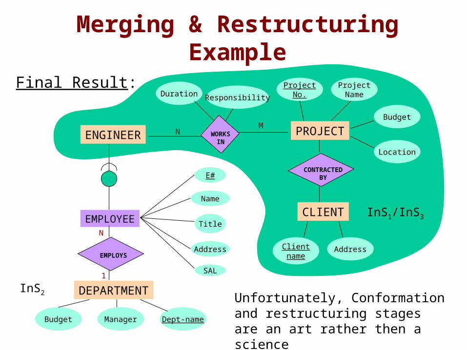
Merging & Restructuring Example
ProjectNo.
ProjectName
Budget
Location
Duration
AddressClientname
ENGINEER WORKSIN
CONTRACTEDBY
CLIENT
MN
N
1
Final Result:
EMPLOYEE
EMPLOYS
E#
Name
Title
SAL
Address
Dept-nameBudget Manager
DEPARTMENTInS2
InS1/InS3
Unfortunately, Conformation and restructuring stages are an art rather then a science
Responsibility
PROJECT
Query Processing inMultidatabase Systems
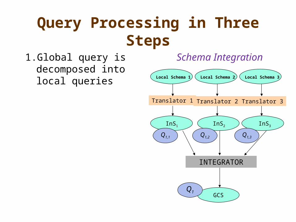
Query Processing in Three Steps
1. Global query is decomposed into local queries Local Schema 1 Local Schema 2 Local Schema 3
Translator 1 Translator 2 Translator 3
InS1
INTEGRATOR
GCS
InS3InS2
Schema Integration
Q1
Q1,1 Q1,2 Q1,3
Query Processing in Three Steps
2. Each local query is translated into queries over the corresponding local database system
Local Schema 1 Local Schema 2 Local Schema 3
Translator 1 Translator 2 Translator 3
InS1
INTEGRATOR
GCS
InS3InS2
Schema Integration
Q1
Q1,1 Q1,2 Q1,3
Q’1,
1
Q’1,2Q’1,3
Query Processing in Three Steps
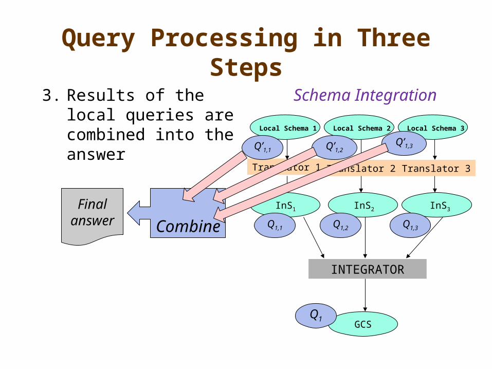
3. Results of the local queries are combined into the answer
Local Schema 1 Local Schema 2 Local Schema 3
Translator 1 Translator 2 Translator 3
InS1
INTEGRATOR
GCS
InS3InS2
Schema Integration
Q1
Q1,1 Q1,2 Q1,3
Q’1,
1
Q’1,2Q’1,3
Combine
Finalanswer
Query Processing in Three Steps
1. Global query is decomposed into local queries
2. Each local query is translated into queries over the corresponding local database system
3. Results of the local queries are combined into the answer
Local Schema 1 Local Schema 2 Local Schema 3
Translator 1 Translator 2 Translator 3
InS1
INTEGRATOR
GCS
InS3InS2
Schema Integration
Outline
• Overview of major query processing components in multidatabase systems:– Query Decomposition– Query Translation– Global Query Optimization
• Techniques for each of the above components
Query Decomposition
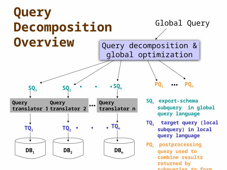
Query DecompositionOverview
Global Query
Query decomposition &global optimization
SQ1 SQ2SQn
. . .Querytranslator 1
Querytranslator 2
Querytranslator n
TQ1 TQ2TQn
DB1 DB2 DBn
. . .
…
PQ1 PQn…
SQi export-schema subquery in global query language
TQi target query (local subquery) in local query language
PQi postprocessing query used to combine results returned by subqueries to form the answer
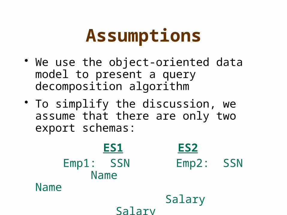
Assumptions• We use the object-oriented data model
to present a query decomposition algorithm
• To simplify the discussion, we assume that there are only two export schemas:
ES1 ES2 Emp1: SSN Emp2: SSN
Name Name Salary Salary Age Rank
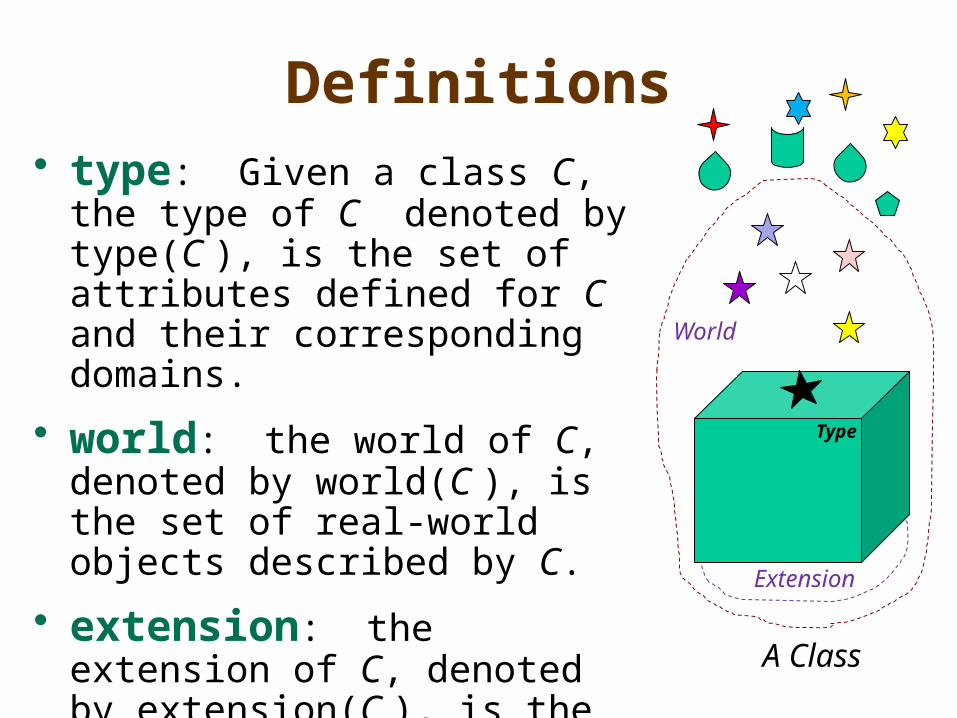
Definitions• type: Given a class C, the
type of C denoted by type(C ), is the set of attributes defined for C and their corresponding domains.
• world: the world of C, denoted by world(C ), is the set of real-world objects described by C.
• extension: the extension of C, denoted by extension(C ), is the set of instances contained in C.
Extension
Type
A Class
World
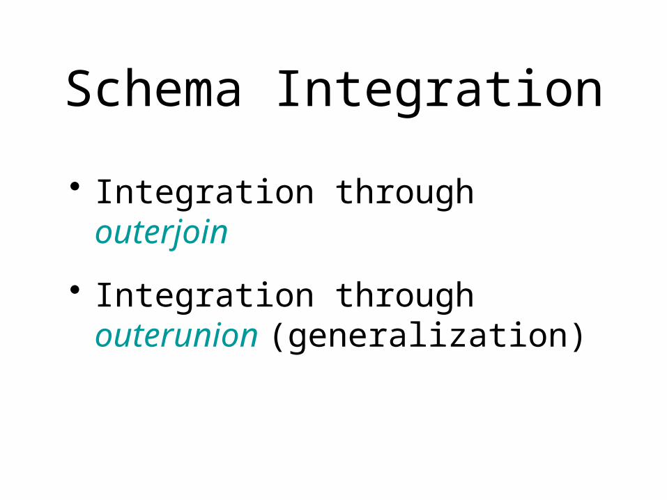
Schema Integration
• Integration through outerjoin
• Integration through outerunion (generalization)
Review: Outerjoin
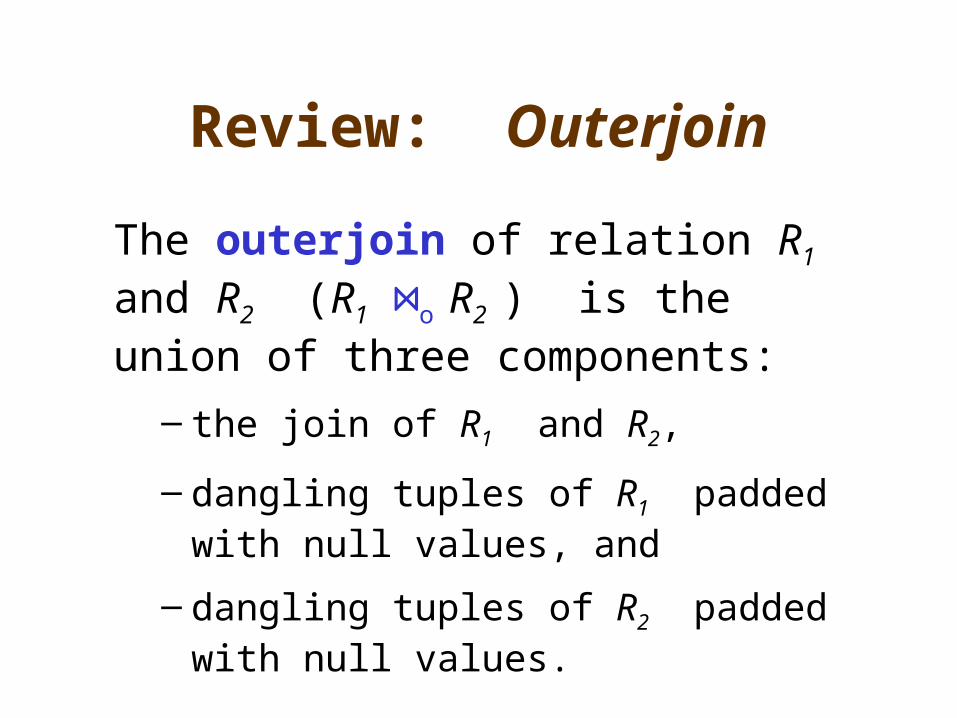
The outerjoin of relation R1 and R2 (R1 ⋈o R2 ) is the union of three components:
– the join of R1 and R2,
– dangling tuples of R1 padded with null values, and
– dangling tuples of R2 padded with null values.
Outerjoin Example
OID SSN Name Salary Age
3 6789 Smith 90,000 40
4 4321 Chang 62,000 30
5 8642 Patel 75,000 35
OID SSN Name Salary Rank
1 2222 Ahad 98,000 S. Mgr.
2 7531 Wang 95,000 S. Mgr.
3 6789 Smith 25,000 Mgr.
OID SSN Name Salary Age Rank
1 2222 Ahad 98,000 null S. Mgr.
2 7531 Wang 95,000 mull S. Mgr.
3 6789 Smith
Incon-
sistent
40 Mgr.
4 4321 Chang 62,000 30 null
5 8642 Patel 75,000 35 null
Emp1
Emp2
Dangling Tuple Dangling Tuple
EmpO = Emp1 ⋈o Emp2

Outerunion
OID SSN Name Salary Age
3 6789 Smith 90,000 40
4 4321 Chang 62,000 30
5 8642 Patel 75,000 35
OID SSN Name Salary Rank
1 2222 Ahad 98,000 S. Mgr.
2 7531 Wang 95,000 S. Mgr.
3 6789 Smith 25,000 Mgr.
OID SSN Name Salary Age Rank
1 2222 Ahad 98,000 null S. Mgr.
2 7531 Wang 95,000 mull S. Mgr.
3 6789 Smith Conflict null Mgr.
3 6789 Smith Conflict 40 null
4 4321 Chang 62,000 30 null
5 8642 Patel 75,000 35 null
Emp1
Emp2
EmpG = Emp1 Uo Emp2
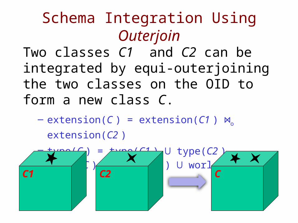
Schema Integration Using Outerjoin
Two classes C1 and C2 can be integrated by equi-outerjoining the two classes on the OID to form a new class C.
– extension(C ) = extension(C1 ) ⋈o
extension(C2 )
– type(C ) = type(C1 ) ⋃ type(C2 )– world(C ) = world(C1 ) ⋃ world(C2 )
C1 C2 C
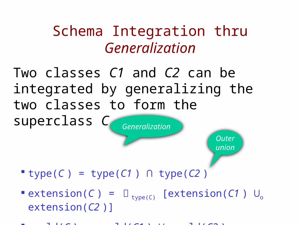
Schema Integration thru Generalization
Two classes C1 and C2 can be integrated by generalizing the two classes to form the superclass C.
type(C ) = type(C1 ) ⋂ type(C2 )
extension(C ) = ᅲ type(C) [extension(C1 ) ⋃o extension(C2 )]
world(C ) = world(C1 ) ⋃ world(C2 )
Outer union
Generalization
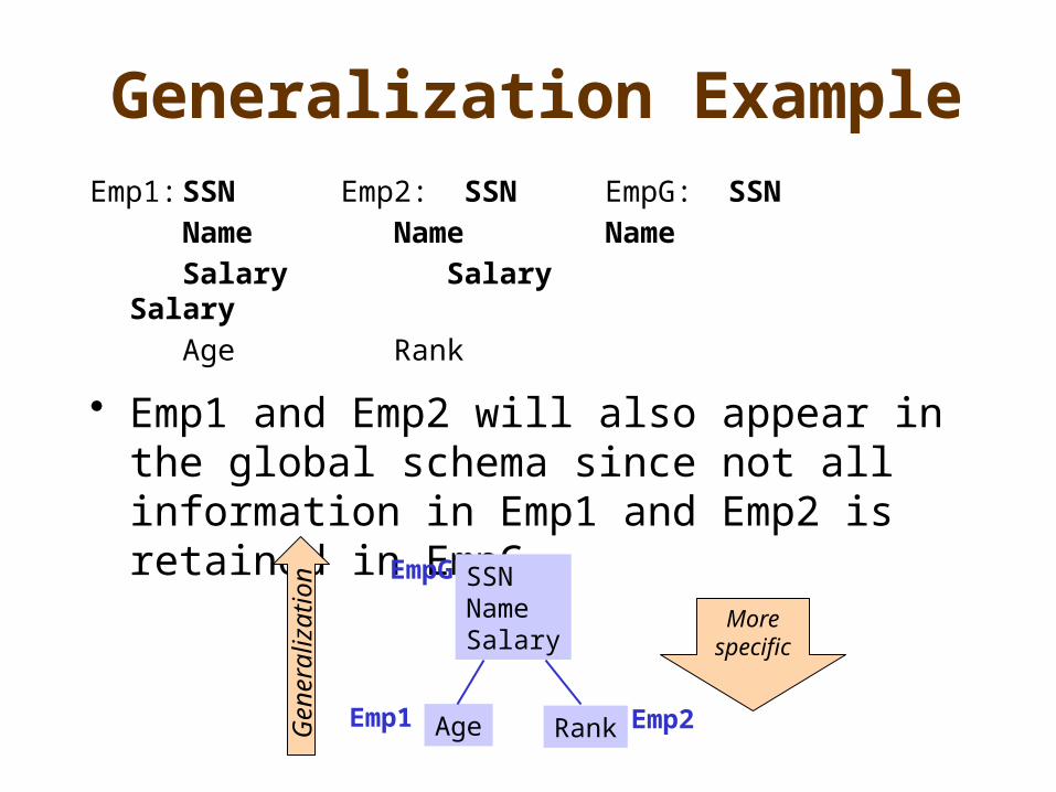
Generalization ExampleEmp1: SSN Emp2: SSN EmpG: SSN
Name Name Name Salary Salary
SalaryAge Rank
• Emp1 and Emp2 will also appear in the global schema since not all information in Emp1 and Emp2 is retained in EmpG
SSNNameSalary
Age Rank
EmpG
Emp2Emp1Genera
lizati
o n
Morespecific
Inconsistency Resolution
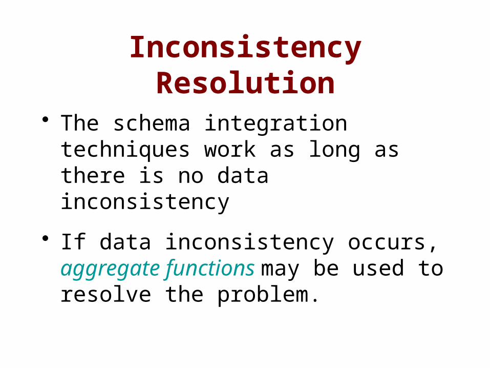
• The schema integration techniques work as long as there is no data inconsistency
• If data inconsistency occurs, aggregate functions may be used to resolve the problem.
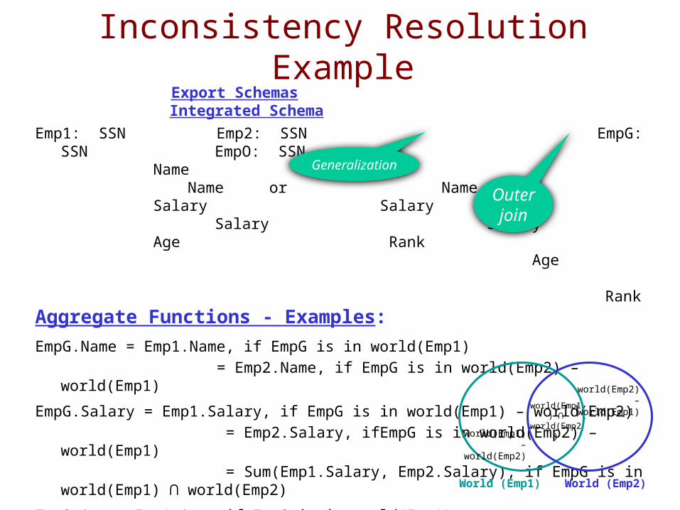
Export Schemas Integrated Schema
Emp1: SSN Emp2: SSN EmpG: SSN EmpO: SSN
Name Name Name or Name
Salary Salary Salary Salary
Age Rank Age
Rank
Aggregate Functions - Examples:
EmpG.Name = Emp1.Name, if EmpG is in world(Emp1) = Emp2.Name, if EmpG is in world(Emp2) – world(Emp1)
EmpG.Salary = Emp1.Salary, if EmpG is in world(Emp1) – world(Emp2) = Emp2.Salary, ifEmpG is in world(Emp2) – world(Emp1) = Sum(Emp1.Salary, Emp2.Salary), if EmpG is in world(Emp1) ⋂
world(Emp2)
EmpO.Age = Emp1.Age, if EmpO is in world(Emp1) = Null, if EmpO is in world(Emp2) – world(Emp1)
EmpO.Rank = Emp2.Rank, if EmpO is in world(Emp2) = Null, if EmpO is in world(Emp1) – world(Emp2)
Inconsistency Resolution Example
World (Emp1) World (Emp2)
world(Emp2) –
world(Emp1)
world(Emp1) –
world(Emp2)
world(Emp1) ⋂
world(Emp2)
Generalization
Outer join
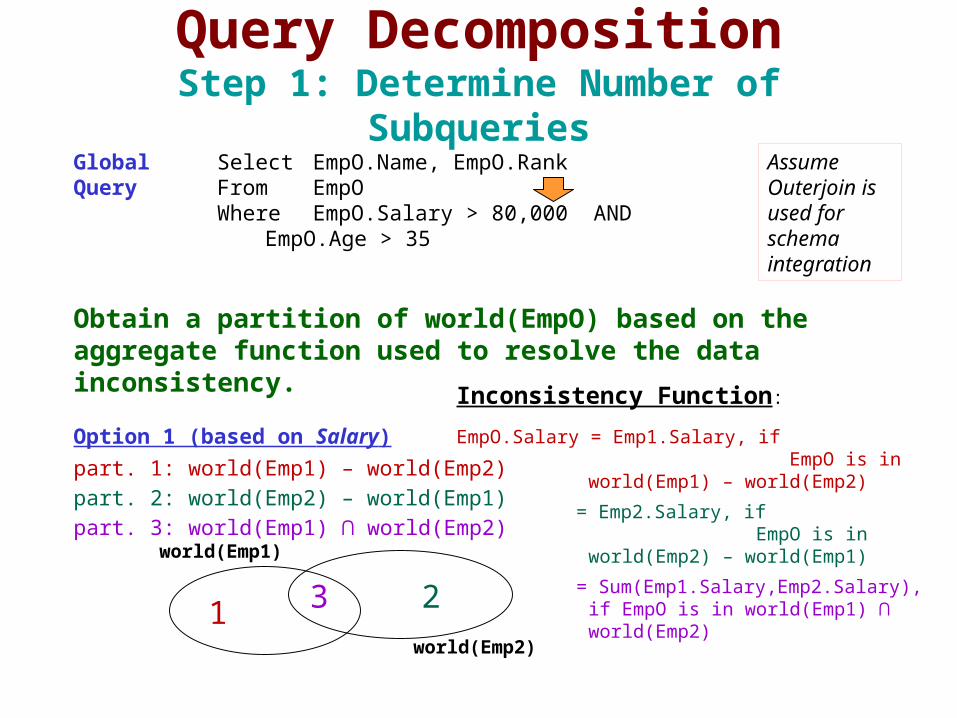
Query DecompositionStep 1: Determine Number of
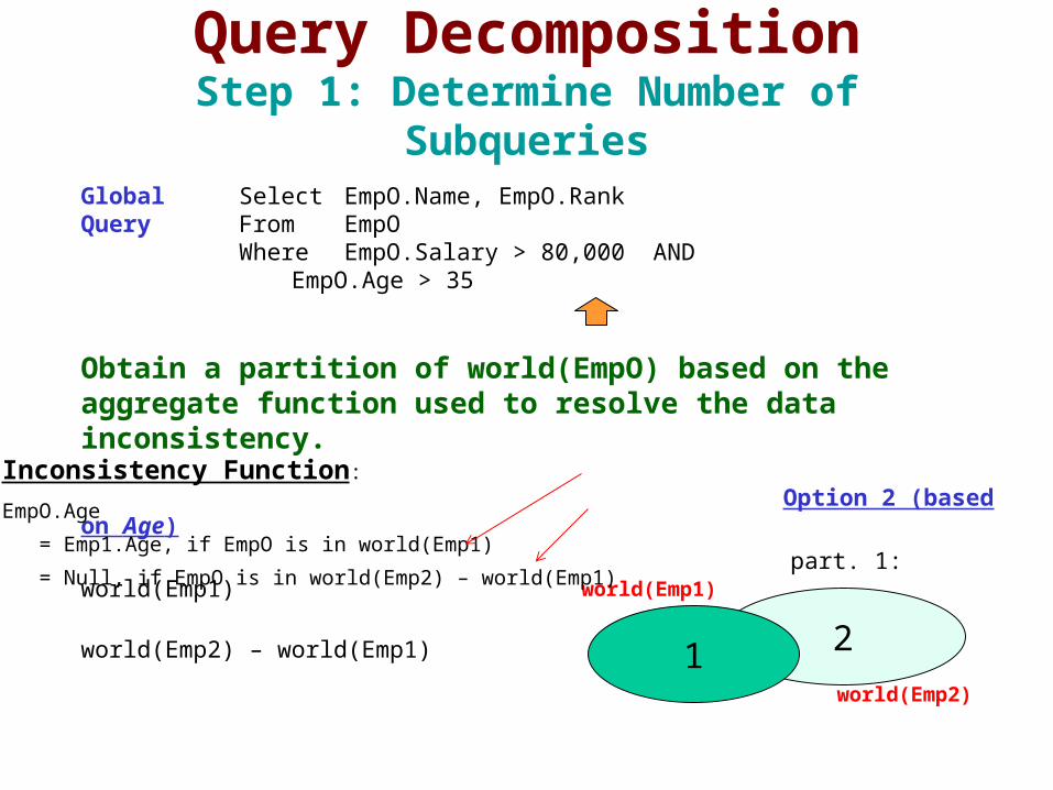
SubqueriesGlobal Select EmpO.Name, EmpO.RankQuery From EmpO
Where EmpO.Salary > 80,000 ANDEmpO.Age > 35
Obtain a partition of world(EmpO) based on the aggregate function used to resolve the data inconsistency.
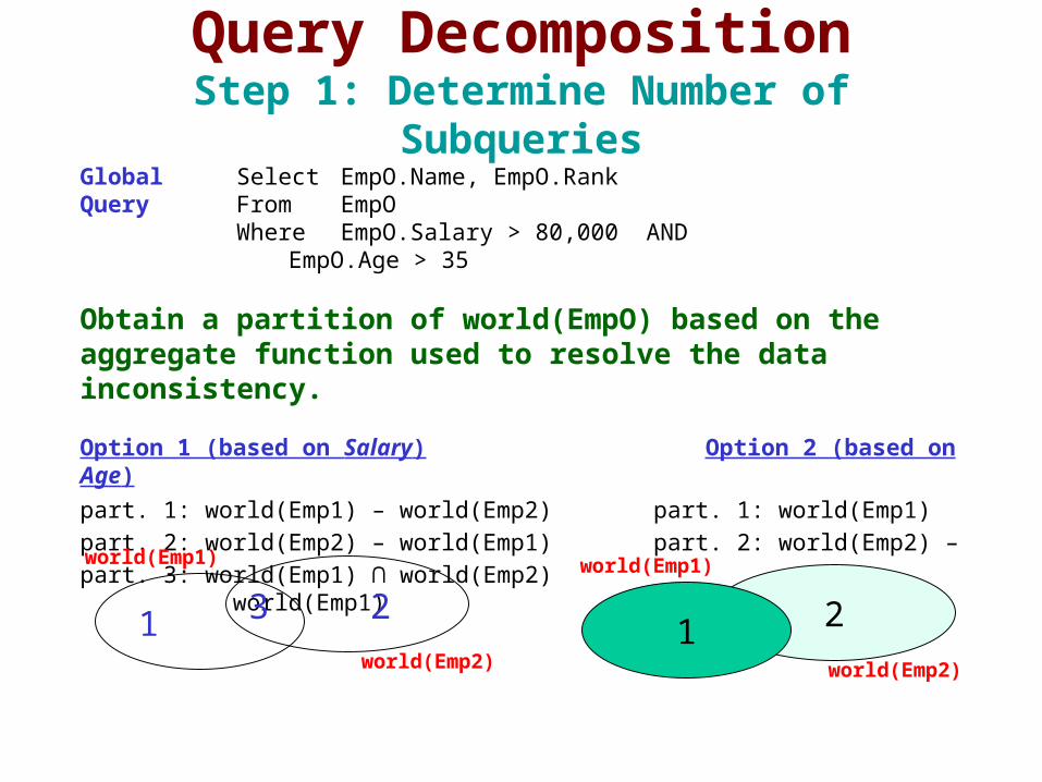
Option 1 (based on Salary)
part. 1: world(Emp1) – world(Emp2)part. 2: world(Emp2) – world(Emp1) part. 3: world(Emp1) ⋂ world(Emp2)
1 3 2
world(Emp1)
world(Emp2)
Inconsistency Function:
EmpO.Salary = Emp1.Salary, if EmpO is in world(Emp1) – world(Emp2)
= Emp2.Salary, if EmpO is in world(Emp2) – world(Emp1)
= Sum(Emp1.Salary,Emp2.Salary), if EmpO is in world(Emp1) ⋂ world(Emp2)
Assume Outerjoin is used for schema integration
Query DecompositionStep 1: Determine Number of
SubqueriesGlobal Select EmpO.Name, EmpO.RankQuery From EmpO
Where EmpO.Salary > 80,000 ANDEmpO.Age > 35
Obtain a partition of world(EmpO) based on the aggregate function used to resolve the data inconsistency.
Option 2 (based on Age)
part. 1: world(Emp1) part. 2: world(Emp2) –
world(Emp1)
21
world(Emp1)
world(Emp2)
Inconsistency Function:
EmpO.Age
= Emp1.Age, if EmpO is in world(Emp1)
= Null, if EmpO is in world(Emp2) – world(Emp1)
Query DecompositionStep 1: Determine Number of
SubqueriesGlobal Select EmpO.Name, EmpO.RankQuery From EmpO
Where EmpO.Salary > 80,000 ANDEmpO.Age > 35
Obtain a partition of world(EmpO) based on the aggregate function used to resolve the data inconsistency.
Option 1 (based on Salary) Option 2 (based on Age)
part. 1: world(Emp1) – world(Emp2) part. 1: world(Emp1)part. 2: world(Emp2) – world(Emp1) part. 2: world(Emp2) – part. 3: world(Emp1) ⋂ world(Emp2) world(Emp1)
We use Option 1 since it is the finest partition among all the partitions.
1 3 2
world(Emp1)
world(Emp2)
21
world(Emp1)
world(Emp2)
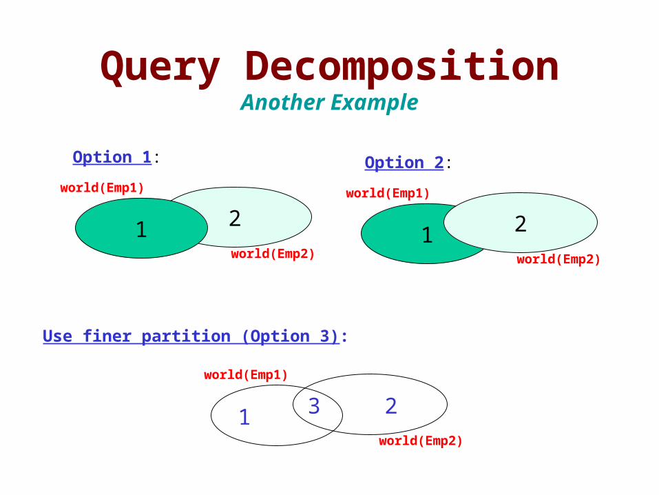
Query DecompositionAnother Example
1 3 2
world(Emp1)
world(Emp2)
21
world(Emp1)
world(Emp2)1
world(Emp1)
world(Emp2)
2
Option 1: Option 2:
Use finer partition (Option 3):
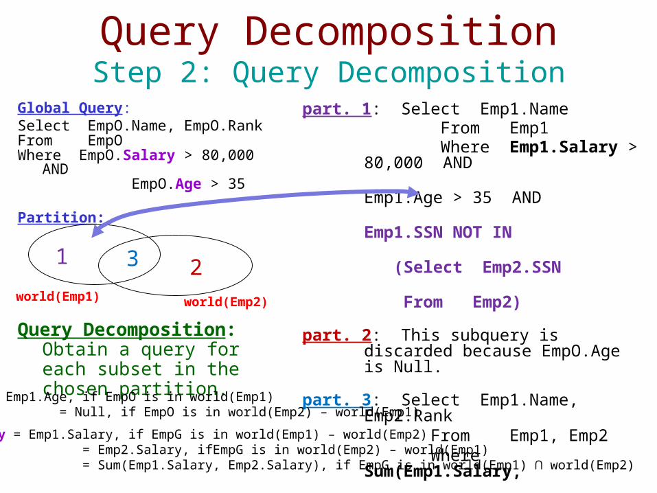
Query DecompositionStep 2: Query Decomposition
Global Query:Select EmpO.Name, EmpO.RankFrom EmpOWhere EmpO.Salary > 80,000
AND EmpO.Age > 35
Partition:
Query Decomposition: Obtain a query for each subset in the chosen partition.
part. 1: Select Emp1.Name From Emp1 Where Emp1.Salary > 80,000
AND Emp1.Age > 35 AND Emp1.SSN NOT IN (Select
Emp2.SSN From
Emp2)
part. 2: This subquery is discarded because EmpO.Age is Null.
part. 3: Select Emp1.Name, Emp2.Rank
From Emp1, Emp2 Where Sum(Emp1.Salary,
Emp2.Salary) >
80,000 AND Emp1.Age > 35 AND Emp1.SSN =
Emp2.SSN
1 3 2world(Emp1) world(Emp2)
EmpO.Age = Emp1.Age, if EmpO is in world(Emp1) = Null, if EmpO is in world(Emp2) – world(Emp1)
EmpO.Salary = Emp1.Salary, if EmpG is in world(Emp1) – world(Emp2) = Emp2.Salary, ifEmpG is in world(Emp2) – world(Emp1) = Sum(Emp1.Salary, Emp2.Salary), if EmpG is in world(Emp1) ⋂ world(Emp2)
Query DecompositionStep 2: Query Decomposition
Global Query:Select EmpO.Name, EmpO.RankFrom EmpOWhere EmpO.Salary > 80,000
AND EmpO.Age > 35
Query Decomposition: Obtain a query for each subset in the chosen partition.
part. 1: Select Emp1.Name From Emp1 Where Emp1.Salary > 80,000
AND Emp1.Age > 35 AND Emp1.SSN NOT IN (Select
Emp2.SSN From
Emp2)
part. 2: This subquery is discarded because EmpO.Age is Null.
part. 3: Select Emp1.Name, Emp2.Rank
From Emp1, Emp2 Where Sum(Emp1.Salary,
Emp2.Salary) >
80,000 AND Emp1.Age > 35 AND Emp1.SSN =
Emp2.SSN
13
2
world(Emp1) world(Emp2)
Emp1.Age
Emp1.Salary
Emp1.Age
Emp1.Salary + Emp2.Salary
Age = nullEmp2.Salary
Query Modification
Query DecompositionStep 3: Further Decomposition
Before STEP 3:Select Emp1.NameFrom Emp1Where Emp1.Salary > 80,000
and Emp1. Age > 35 and Emp1.SSN NOT IN (Select Emp2.SSN From Emp2)
Select Emp1.NameFrom Emp1Where Emp1.Salary > 80,000
and Emp1. Age > 35 and Emp1.SSN NOT IN X
Insert INTO XSelect Emp2.SSNFrom Emp2)
STEP 3: Some resulting query may still reference data from more than one database. They need to be further decomposed into subqueries and possibly also postprocessing queries
X
Query DecompositionStep 4: Query Optimization
STEP 4: It may be desirable to reduce the number of subqueries by combining subqueries for the same database.

Query Translation
Query Translation (1)
IF Global Query Language ≠Local Query Language
THEN Export Local Schema Query Subquery
Language
Translator
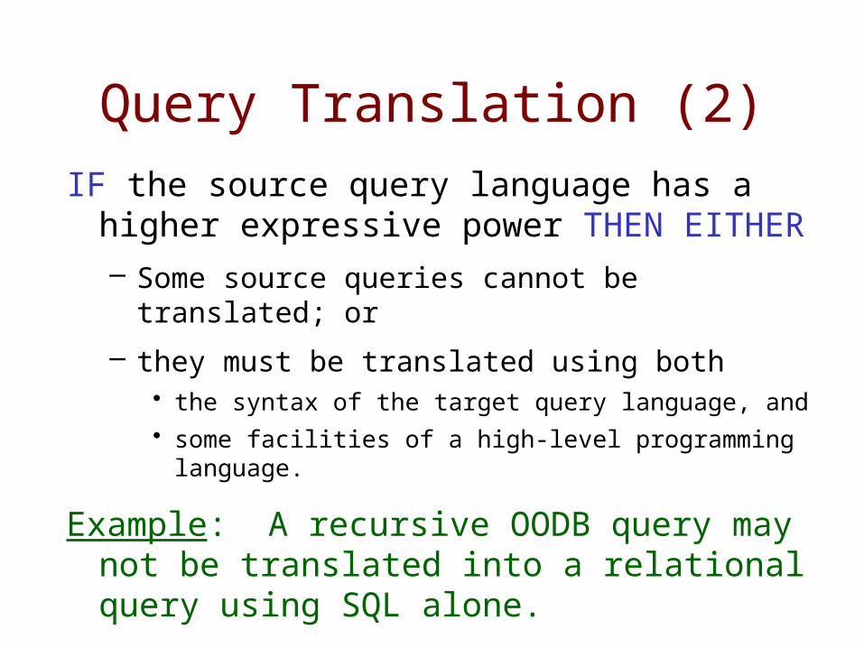
Query Translation (2)IF the source query language has a higher
expressive power THEN EITHER– Some source queries cannot be translated; or
– they must be translated using both• the syntax of the target query language, and• some facilities of a high-level programming language.
Example: A recursive OODB query may not be translated into a relational query using SQL alone.
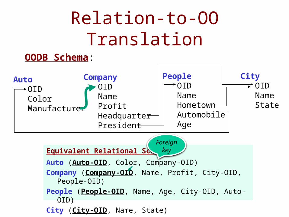
Relation-to-OO Translation
Equivalent Relational Schema:
Auto (Auto-OID, Color, Company-OID)Company (Company-OID, Name, Profit, City-OID,
People-OID)People (People-OID, Name, Age, City-OID, Auto-OID)City (City-OID, Name, State)
OODB Schema:
Auto OID Color Manufacturer
Company OID Name Profit Headquarter President
People OID Name Hometown Automobile Age
City OID Name State
Foreign key
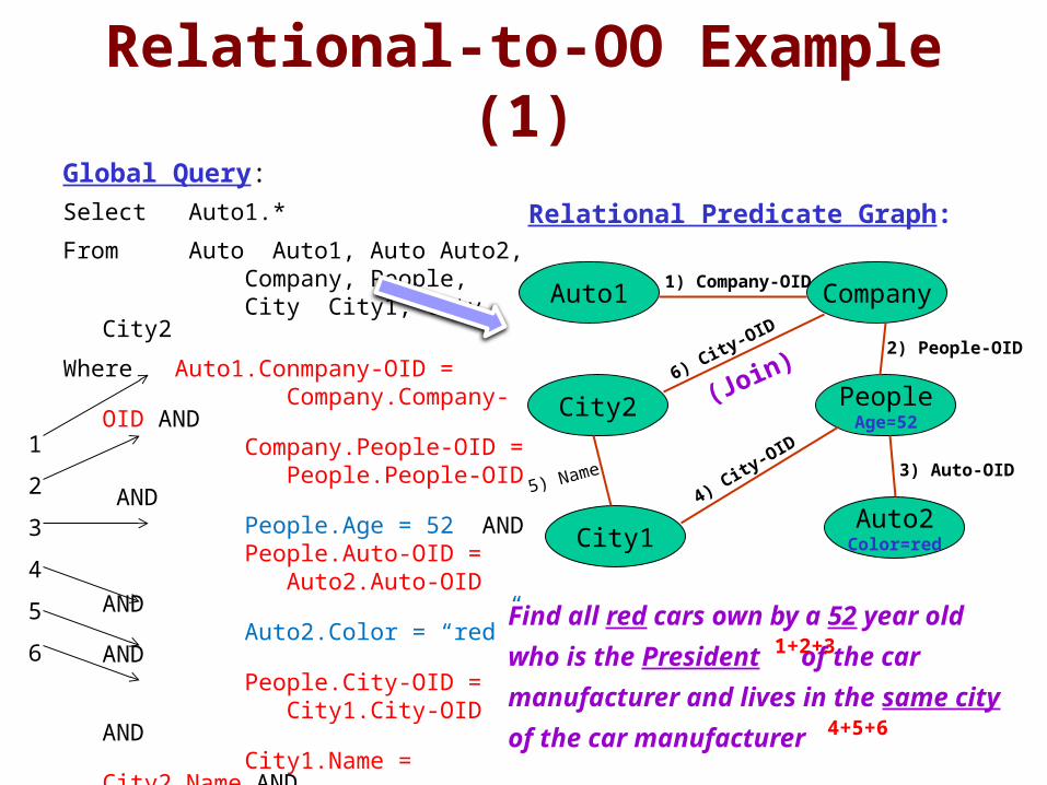
Relational-to-OO Example (1)
Global Query:Select Auto1.*
From Auto Auto1, Auto Auto2, Company, People, City City1, City City2
Where Auto1.Conmpany-OID = Company.Company-OID AND Company.People-OID = People.People-OID AND People.Age = 52 AND People.Auto-OID = Auto2.Auto-OID AND Auto2.Color = “red” AND People.City-OID = City1.City-OID AND City1.Name = City2.Name AND Company.City-OID = City2.City-OID
Relational Predicate Graph:
Auto1 Company
City2
City1
PeopleAge=52
Auto2Color=red
1) Company-OID
4) City
-OID
2) People-OID
3) Auto-OID
Find all red cars own by a 52 year
old who is the President of the
car manufacturer and lives in the
same city of the car manufacturer
1
2
3
4
5
6
5) Name
1+2+3
4+5+6
6) City
-OID
(Join)
Relational-to-OO Example (2)
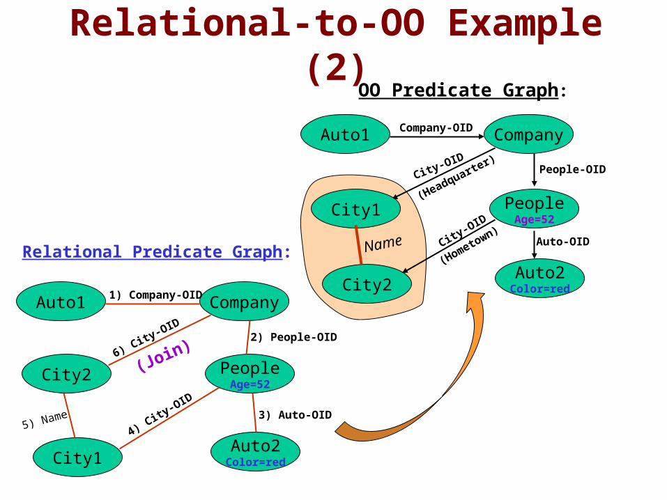
OO Predicate Graph:
Auto1 Company
City2
PeopleAge=52
Auto2Color=red
Company-OID
City-O
ID
People-OID
Auto-OID
City1
City-OID
(Headquarte
r)
(Hometo
wn)
NameRelational Predicate Graph:
Auto1 Company
City2
City1
PeopleAge=52
Auto2Color=red
1) Company-OID
4) City
-OID
2) People-OID
3) Auto-OID5) Name
6) City
-OID
(Join)
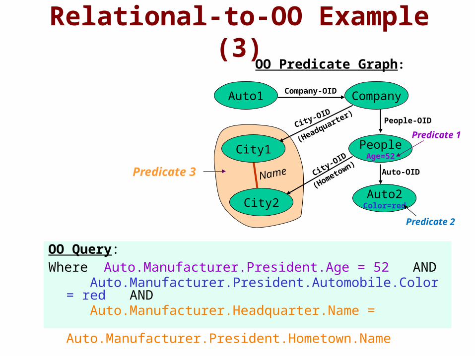
Relational-to-OO Example (3)
OO Query:Where Auto.Manufacturer.President.Age = 52 AND
Auto.Manufacturer.President.Automobile.Color = red AND
Auto.Manufacturer.Headquarter.Name =
Auto.Manufacturer.President.Hometown.Name
OO Predicate Graph:
Auto1 Company
City2
PeopleAge=52
Auto2Color=red
Company-OID
City-O
ID
People-OID
Auto-OID
City1
Predicate 3
Predicate 1
Predicate 2
City-OID
(Headquarte
r)
(Hometo
wn)
Name

Global Query Optimization
Query Optimization (1)
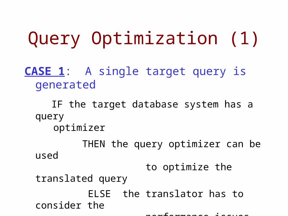
CASE 1: A single target query is generated
IF the target database system has a query optimizer
THEN the query optimizer can be used to optimize the translated query
ELSE the translator has to consider the performance issues
Query Optimization (2)
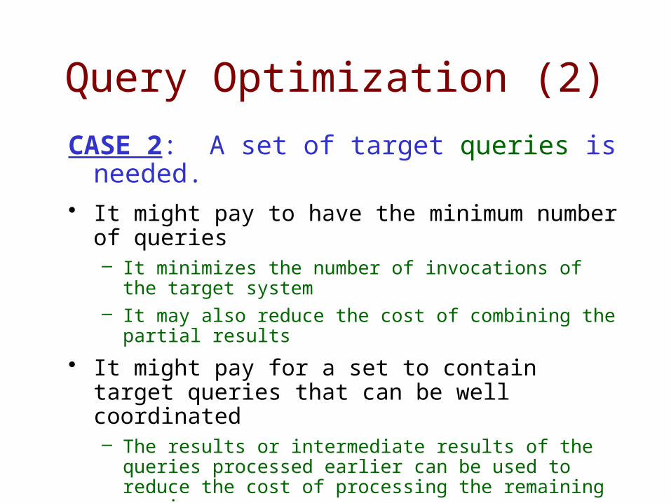
CASE 2: A set of target queries is needed.
• It might pay to have the minimum number of queries– It minimizes the number of invocations of the target
system– It may also reduce the cost of combining the partial
results
• It might pay for a set to contain target queries that can be well coordinated– The results or intermediate results of the queries
processed earlier can be used to reduce the cost of processing the remaining queries
Global Query Optimization (1)
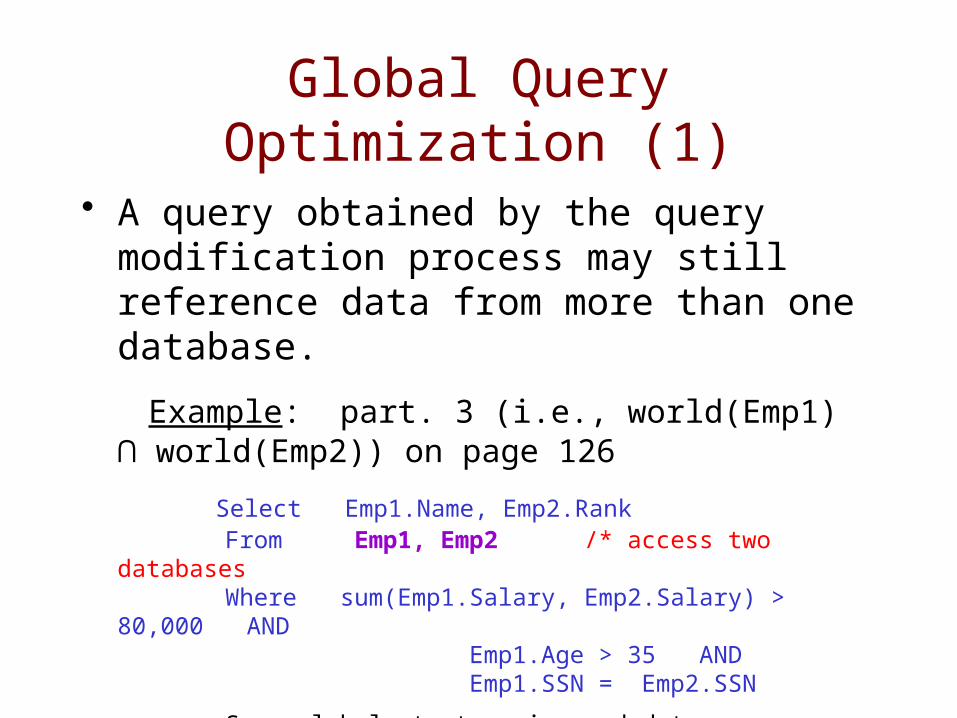
• A query obtained by the query modification process may still reference data from more than one database.
Example: part. 3 (i.e., world(Emp1) ⋂ world(Emp2)) on page 126
Select Emp1.Name, Emp2.Rank From Emp1, Emp2 /* access two databases Where sum(Emp1.Salary, Emp2.Salary) > 80,000 AND Emp1.Age > 35 AND Emp1.SSN = Emp2.SSN
→ Some global strategy is needed to process such queries
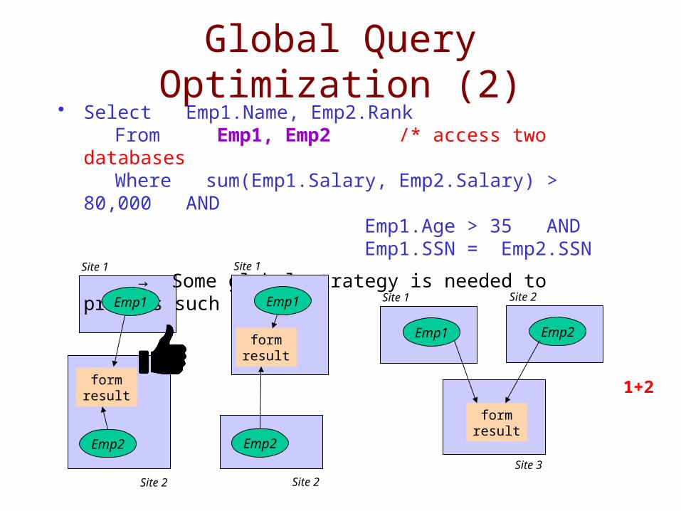
Global Query Optimization (2)
• Select Emp1.Name, Emp2.Rank From Emp1, Emp2 /* access two databases Where sum(Emp1.Salary, Emp2.Salary) > 80,000
AND Emp1.Age > 35 AND Emp1.SSN = Emp2.SSN
→ Some global strategy is needed to process such queries
Emp1
formresult
Emp2
Site 1
Site 2
Emp1
formresult
Emp2
Site 1
Site 2
Emp1
Site 1
Emp2
Site 2
formresult
Site 3
1+2
OID SSN Name Salary Age Rank
1 2222 Ahad 98,000 null S. Mgr.
2 7531 Wang 95,000 mull S. Mgr.
3 6789 Smith
Incon-
sistent
40 Mgr.
4 4321 Chang 62,000 30 null
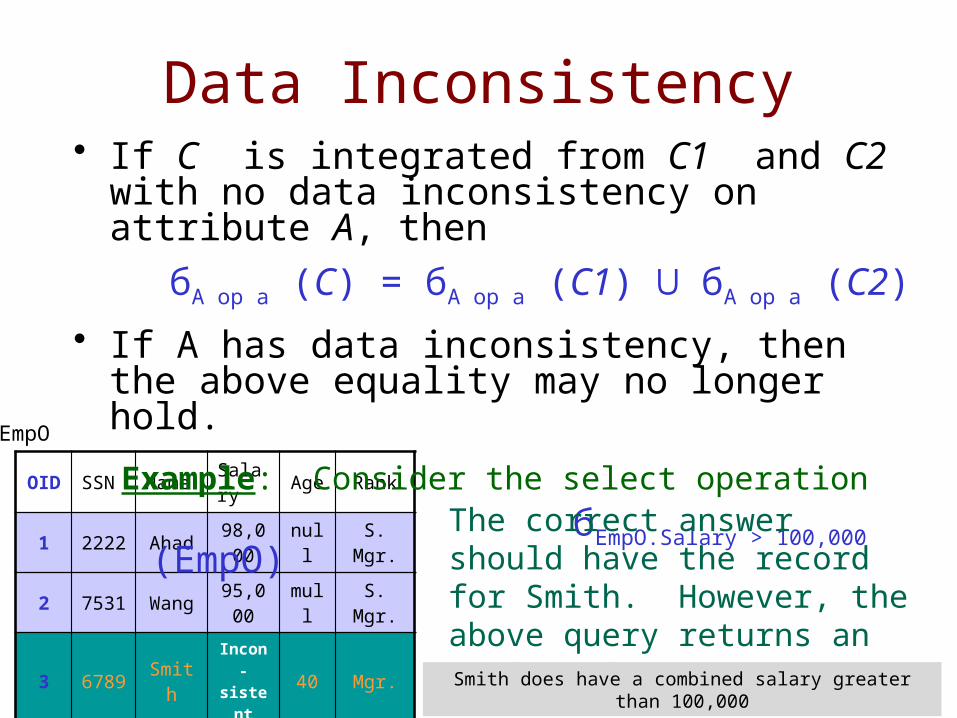
5 8642 Patel 75,000 35 null
Data Inconsistency• If C is integrated from C1 and C2 with no
data inconsistency on attribute A, then
бA op a (C) = бA op a (C1) ⋃ бA op a (C2)
• If A has data inconsistency, then the above equality may no longer hold.
Example: Consider the select operation бEmpO.Salary > 100,000
(EmpO)
EmpO
The correct answer should have the record for Smith. However, the above query returns an empty setSmith does have a combined salary greater than
100,000
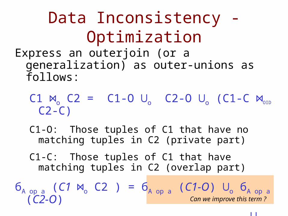
Data Inconsistency - Optimization
Express an outerjoin (or a generalization) as outer-unions as follows:
C1 ⋈o C2 = C1-O ⋃o C2-O ⋃o (C1-C ⋈OID C2-C)
C1-O: Those tuples of C1 that have no matching tuples in C2 (private part)
C1-C: Those tuples of C1 that have matching tuples in C2 (overlap part)
бA op a (C1 ⋈o C2 ) = бA op a (C1-O) ⋃o бA op a (C2-O)
⋃o бA op a (C1-C ⋈ C2-C)Can we improve this term ?
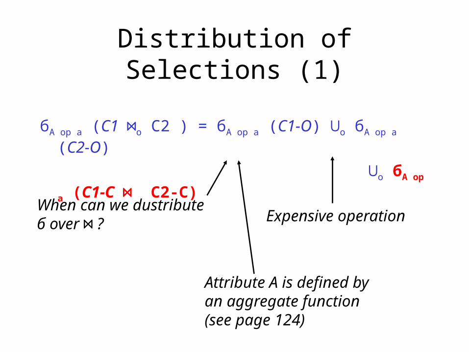
Distribution of Selections (1)
бA op a (C1 ⋈o C2 ) = бA op a (C1-O) ⋃o бA op a (C2-O)
⋃o бA op a (C1-C ⋈ C2-C)
When can we dustributeб over ⋈ ? Expensive operation
Attribute A is defined byan aggregate function(see page 124)
Distribution of Selection (2)
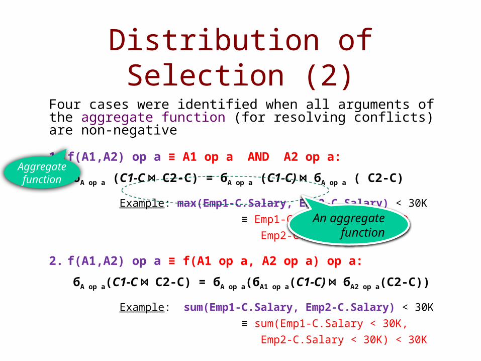
Four cases were identified when all arguments of the aggregate function (for resolving conflicts) are non-negative
1. f(A1,A2) op a ≡ A1 op a AND A2 op a:
бA op a (C1-C ⋈ C2-C) = бA op a (C1-C) ⋈ бA op a ( C2-C)
Example: max(Emp1-C.Salary, Emp2-C.Salary) < 30K
≡ Emp1-C.Salary < 30K AND
Emp2-C.Salary < 30K
2. f(A1,A2) op a ≡ f(A1 op a, A2 op a) op a:
бA op a(C1-C ⋈ C2-C) = бA op a(бA1 op a(C1-C) ⋈ бA2 op a(C2-C))
Example: sum(Emp1-C.Salary, Emp2-C.Salary) < 30K
≡ sum(Emp1-C.Salary < 30K,
Emp2-C.Salary < 30K) < 30K
Aggregate function
An aggregate
function
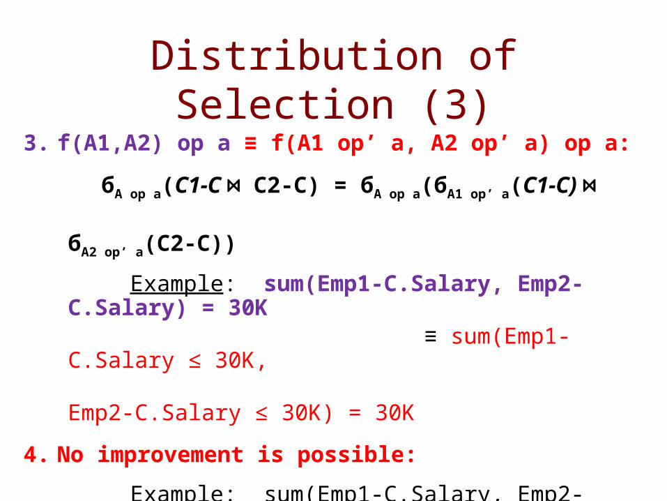
Distribution of Selection (3)
3. f(A1,A2) op a ≡ f(A1 op’ a, A2 op’ a) op a:
бA op a(C1-C ⋈ C2-C) = бA op a(бA1 op’ a(C1-C) ⋈
бA2 op’ a(C2-C))
Example: sum(Emp1-C.Salary, Emp2-C.Salary) = 30K
≡ sum(Emp1-C.Salary ≤ 30K, Emp2-C.Salary ≤ 30K) = 30K
4. No improvement is possible:
Example: sum(Emp1-C.Salary, Emp2-C.Salary) > 30K
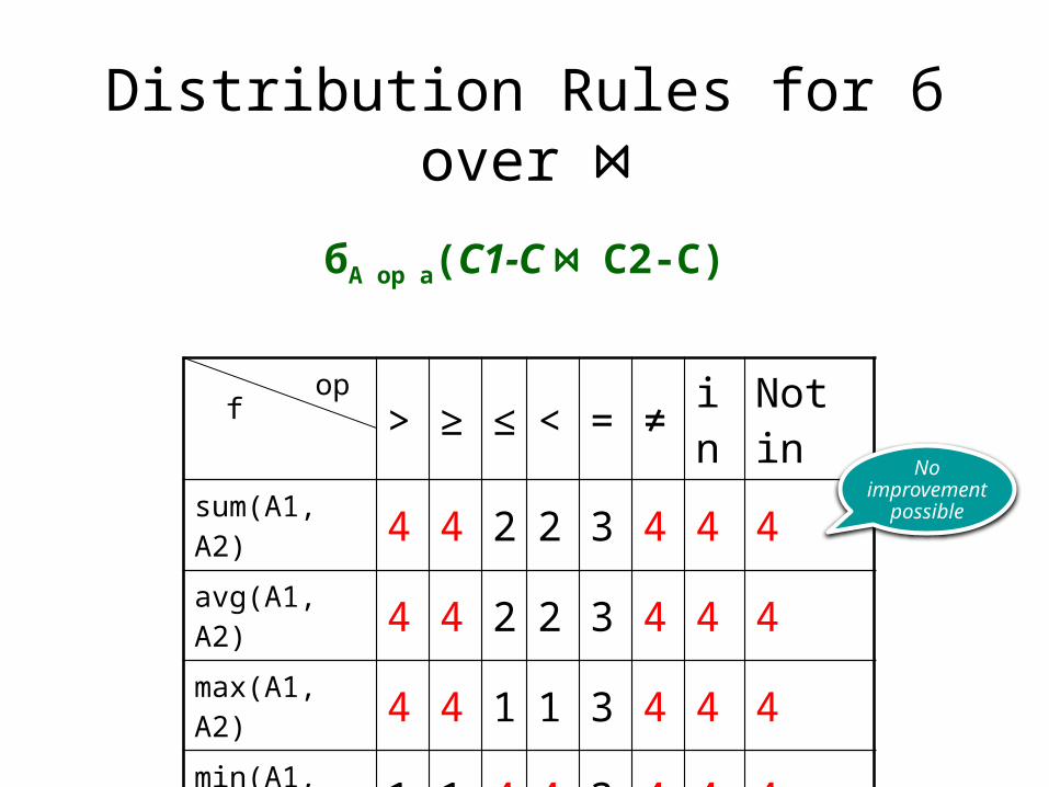
Distribution Rules for б over ⋈
бA op a(C1-C ⋈ C2-C)
> ≥ ≤ < = ≠ in Not in
sum(A1, A2) 4 4 2 2 3 4 4 4
avg(A1, A2) 4 4 2 2 3 4 4 4
max(A1, A2) 4 4 1 1 3 4 4 4
min(A1, A2) 1 1 4 4 3 4 4 4
opf
No improvement possible
Problem in Global Query Optimization (1)
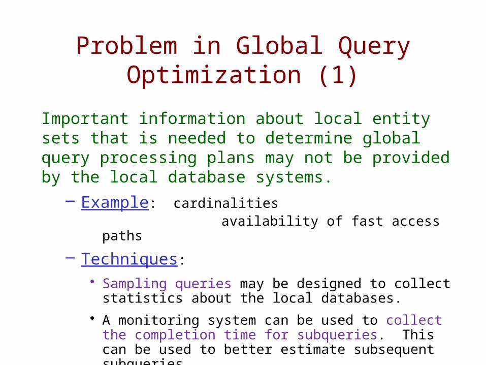
Important information about local entity sets that is needed to determine global query processing plans may not be provided by the local database systems.
– Example: cardinalities availability of fast access paths
– Techniques:
• Sampling queries may be designed to collect statistics about the local databases.
• A monitoring system can be used to collect the completion time for subqueries. This can be used to better estimate subsequent subqueries.
Problems in Global Query Optimization (2)
• Different query processing algorithms may have been used in different local database systems.→ Cooperation across different systems difficult Examples: Semijoin may not be supported on some local systems.
• Data transmission between different local database systems may not be fully supported.Examples:– A local database system may not allow update
operations– For many nonrelational systems, the instances of one
entity set are more likely to be clustered with the instances of other entity sets. Such clustering makes it very expensive to extract data for one entity set.
→ Need more sophisticated decomposition algorithms.