Distributed Control of Electric Drives via Ethernet - DiVA Portal
108
TRITA-ETS-2003-09 ISSN 1650–674x ISRN KTH/EME/R 0305-SE Distributed Control of Electric Drives via Ethernet Lilantha Samaranayake Royal Institute of Technology Department of Electrical Engineering Electrical Machines and Power Electronics Stockholm 2003
Transcript of Distributed Control of Electric Drives via Ethernet - DiVA Portal

TRITA-ETS-2003-09
ISSN 1650–674x
ISRN KTH/EME/R 0305-SE
Distributed Control of Electric Drives
via Ethernet
Lilantha Samaranayake
Royal Institute of Technology
Department of Electrical Engineering
Electrical Machines and Power Electronics
Stockholm 2003

TRITA-ETS-2003-09
ISSN 1650–674x
ISRN KTH/EME/R 0305-SE
This document was prepared using LATEX.

Abstract
This report presents the work carried out aiming towards distributed control
of electric drives through a network communication medium with temporal
constraints, i.e, Ethernet. A general analysis on time delayed systems is
carried out, using state space representation of systems in the discrete time
domain. The effect of input time delays is identified and is used in the
preceding controller designs.
The main hardware application focused in this study is a Brushless DC
servo motor, whose speed control loop is closed via a 10 Mbps Switched
Ethernet network. The speed control loop, which is approximately a decade
slower than the current control loop, is opened and interfaced to the network
at the sensor/actuator node. It is closed at the speed controller end at
another node in the same local area network (LAN) forming a distributed
control system (DCS).
The Proportional Integral (PI) classical controller design technique with
ample changes in parameter tuning suitable for time delayed systems is used.
Then the standard Smith Predictor is tested, modified with the algebraic
design technique Coefficient Diagram Method (CDM), which increases the
system degrees of freedom. Constant control delay is assumed in the latter
designs despite the slight stochastic nature in the timing data observations.
Hence the poor transient performance of the system is the price for the
robustness inherited to the speed controllers at the design stage. The con-
trollability and observability of the DCS may be lost, depending on the range
in which the control delay is varying. However a state feedback controller
i
deploying on-line delay data, obtained by means of synchronizing the sensor
node and controller node system clocks, results in an effective compensation
scheme for the network induced delays. Hence the full state feedback con-
troller makes the distributed system transient performance acceptable for
servo applications with the help of pole placement controller design.
Further, speed synchronizing controllers have been designed such that
a speed fluctuation caused by a mechanical load torque disturbance on one
motor is followed effectively by any other specified motor in the distributed
control network with a minimum tracking or synchronizing error. This type
of performance is often demanded in many industrial applications such as
printing, paper, bagging, pick and place and material cutting.
Keywords
• Brushless DC Motor
• Control Delay
• Distributed Motion Control Systems
• Proportional Integral Controller
• Smith Predictor
• Speed Synchronization
• State Feedback Controller
• Stochastic Systems
• Switched-Ethernet
• Synchronizing Error
• Time Delayed Systems
• Tracking Error
ii
Acknowledgments
First, I would like to thank my main supervisor Prof. Chandur Sadarangani,
for giving me the opportunity to pursue my post graduate studies at the divi-
sion of Electrical Machines and Power Electronics and for his encouragement
to carry on this work.
My special thank goes to Dr. Sanath Alahakoon and Tech. Lic. Mats
Leksell, my co-supervisors, for their relentless discussions on project matters
as well as the other commitments paid towards the project activities, and
also for proof reading this report. My sincere thanks goes to Dr. Juliette
Soulard for providing me home in the Permanent Magnet Drives (PMD) pro-
gram within the division. Constructive project discussions with Dr. Kirthi
Walgama, during my stay in the University of Peradeniya (UP) Sri Lanka,
are also highly appreciated.
The opportunities given for me to explore the jungle of information tech-
nology under the guidance of Mats Westerborn and Stefan Sundquist of IT
university, Kista are remembered gratefully. I must also thank Prof. Martin
Torngren for introducing me to the domain of Real-Time control systems at
the Dept. of Machine Design, Royal Institute of Technology (KTH).
The financial support provided by the Swedish International Develop-
ment cooperation Agency (SIDA) under the “Research capacity building
in Electrical and Electronic Engineering in the University of Peradeniya”,
in collaboration between the Dept. of Electrical Engineering (ETS), KTH,
Sweden and the Dept. of Electrical and Electronic Engineering (DEEE),
UP, Sri Lanka is gratefully acknowledged.
iii

I would like to thank all staff members of EME and DEEE for creating
a friendly working environment and their support in all aspects.
I pay my earnest gratitude to my dear parents, Mr. & Mrs. B. G.
Samaranayake, for their love, care and sacrifices, which made it possible for
me to pursue with higher studies. And also to my sister Lalani and brother
Malinga and all my teachers and friends for encouraging me to continue post
graduate studies. At last but not least, to my wife Upeka for her patience
and understanding throughout.
Stockholm, Spring 2003.
Lilantha Samaranayake
iv

Contents
1 Introduction 1
1.1 Background . . . . . . . . . . . . . . . . . . . . . . . . . . . . 1
1.2 Outline . . . . . . . . . . . . . . . . . . . . . . . . . . . . . . 3
2 Distributed Control Systems 5
2.1 Communication in DCS . . . . . . . . . . . . . . . . . . . . . 6
2.1.1 FIP (Factory Instrumentation Protocol) . . . . . . . . 7
2.1.2 PROFIBUS (Process Fieldbus) . . . . . . . . . . . . . 7
2.1.3 CAN (Controller Area Network) . . . . . . . . . . . . 7
2.2 Ethernet . . . . . . . . . . . . . . . . . . . . . . . . . . . . . . 8
2.2.1 Ethernet model . . . . . . . . . . . . . . . . . . . . . . 10
2.2.2 CSMA/CD access control . . . . . . . . . . . . . . . . 12
2.2.3 Half-duplex . . . . . . . . . . . . . . . . . . . . . . . . 13
2.2.4 Full-duplex . . . . . . . . . . . . . . . . . . . . . . . . 14
2.2.5 Ethernet Switch . . . . . . . . . . . . . . . . . . . . . 14
2.3 Ethernet for real-time applications : A survey . . . . . . . . . 17
2.3.1 RETHER . . . . . . . . . . . . . . . . . . . . . . . . . 17
2.3.2 EtheReal . . . . . . . . . . . . . . . . . . . . . . . . . 18
2.3.3 TEMPRA . . . . . . . . . . . . . . . . . . . . . . . . . 19
2.3.4 SIRTE . . . . . . . . . . . . . . . . . . . . . . . . . . . 19
2.3.5 IPv6 . . . . . . . . . . . . . . . . . . . . . . . . . . . . 20
3 Problem Formulation 23
3.1 Brushless DC motor . . . . . . . . . . . . . . . . . . . . . . . 23
3.2 Local servo amplifier . . . . . . . . . . . . . . . . . . . . . . . 25
3.3 Controller . . . . . . . . . . . . . . . . . . . . . . . . . . . . . 26
v
Contents
3.4 Network . . . . . . . . . . . . . . . . . . . . . . . . . . . . . . 26
3.5 Time delayed system . . . . . . . . . . . . . . . . . . . . . . . 26
3.5.1 Overview . . . . . . . . . . . . . . . . . . . . . . . . . 26
3.5.2 Open loop model . . . . . . . . . . . . . . . . . . . . . 29
3.5.3 Design criteria . . . . . . . . . . . . . . . . . . . . . . 32
4 Analysis of time delayed systems 33
4.1 Timing Analysis . . . . . . . . . . . . . . . . . . . . . . . . . 33
4.1.1 Discrete Time Control System . . . . . . . . . . . . . 36
4.1.2 Effect of time delays . . . . . . . . . . . . . . . . . . . 38
4.1.3 Simulation results . . . . . . . . . . . . . . . . . . . . 39
4.2 Controllability and Observability . . . . . . . . . . . . . . . . 40
4.3 Delay model . . . . . . . . . . . . . . . . . . . . . . . . . . . . 43
5 Controller design for the time delayed system 45
5.1 PI controller . . . . . . . . . . . . . . . . . . . . . . . . . . . . 45
5.1.1 Discretization . . . . . . . . . . . . . . . . . . . . . . . 46
5.1.2 Integrator Wind-Up problem . . . . . . . . . . . . . . 47
5.1.3 Stability Problem . . . . . . . . . . . . . . . . . . . . . 48
5.2 Smith Predictor . . . . . . . . . . . . . . . . . . . . . . . . . . 49
5.2.1 Coefficient Diagram Method (CDM) . . . . . . . . . . 51
5.2.2 Design procedure . . . . . . . . . . . . . . . . . . . . . 52
5.2.3 Design for the test rig . . . . . . . . . . . . . . . . . . 53
5.3 State Feedback Controller . . . . . . . . . . . . . . . . . . . . 54
5.3.1 Analysis . . . . . . . . . . . . . . . . . . . . . . . . . . 54
5.3.2 Timing data acquisition . . . . . . . . . . . . . . . . . 56
5.3.3 Clock synchronization . . . . . . . . . . . . . . . . . . 57
5.3.4 Time stamping . . . . . . . . . . . . . . . . . . . . . . 58
5.3.5 State Feedback Gain . . . . . . . . . . . . . . . . . . . 59
5.3.6 Estimator Design . . . . . . . . . . . . . . . . . . . . . 65
5.3.7 Reference Gain . . . . . . . . . . . . . . . . . . . . . . 67
5.4 Results . . . . . . . . . . . . . . . . . . . . . . . . . . . . . . . 68
6 Speed Synchronization 71
6.1 Introduction . . . . . . . . . . . . . . . . . . . . . . . . . . . . 71
6.2 Application Aspects . . . . . . . . . . . . . . . . . . . . . . . 72
vi

Contents
6.2.1 Offset Printing . . . . . . . . . . . . . . . . . . . . . . 72
6.2.2 Horizontal Bagging . . . . . . . . . . . . . . . . . . . . 72
6.2.3 Cut to Length Rotary Knife . . . . . . . . . . . . . . . 73
6.2.4 Pick and Place . . . . . . . . . . . . . . . . . . . . . . 75
6.3 Approach . . . . . . . . . . . . . . . . . . . . . . . . . . . . . 76
6.3.1 Master Slave . . . . . . . . . . . . . . . . . . . . . . . 76
6.3.2 Interactive Feedback Control . . . . . . . . . . . . . . 77
6.3.3 Synchronization in distributed systems . . . . . . . . . 79
6.4 Reference Feedback Control . . . . . . . . . . . . . . . . . . . 82
7 Conclusions and future work 87
7.1 Conclusions . . . . . . . . . . . . . . . . . . . . . . . . . . . . 87
7.2 Future work . . . . . . . . . . . . . . . . . . . . . . . . . . . . 89
References 91
List of symbols 97
vii

Contents
viii
1 Introduction
1.1 Background
Feedback control systems wherein the control loops are closed through a
network are called distributed control systems (DCS) [1], [2]. The defining
feature of a DCS is that the information (reference input, plant output,
control input, etc.) is exchanged using a communication network running
over the main control system modules (sensors, controllers, actuators, etc.).
Moving one step further, the system becomes truly distributed, when parts
of the accessible inner control loops are handed over to the actuator. For
example in electrical motors, the fast inner current control loop can be closed
in the vicinity of the actuator while the slower speed control loop can be
closed through a network connected speed controller. The basic advantage of
DCS is its capability of controlling many such systems from a single location
at a lower installation and maintenance cost.
However, the insertion of the communication network in the feedback
control loop complicates the analysis and design of the DCS. Conventional
control theories with many ideal assumptions, such as synchronized control,
non delayed sensing and actuation, must be re-evaluated. Specifically the
following issues need to be addressed.
Firstly the network induced delays, mainly the sensor to controller delay
(τsc) and the controller to actuator delay (τca) that occur while exchanging
data among devices connected to the network. These delays, either constant
1

1 Introduction
or time varying [3], can degrade or even destabilize the performance of DCS
unless they are considered in the design [26]. Secondly, the network can be
viewed as a web of unreliable transmission paths. Hence some data packets
can get lost completely in the transmission. Thirdly due to the bandwidth
and packet size constraints of the network, the data may be transmitted
using multiple data packets [4]. Therefore depending on the method of
media access, the number of active nodes operating, the available bandwidth
etc., chances are that all, part or none of the packets could arrive their
destinations on time. Thus the behavior of a DCS is largely dependent
upon the performance parameters of the underlying network. DeviceNet,
CAN and Ethernet are such networks to name and focus in this study is on
Ethernet.
In Ethernet, the packet drop out problem can be solved by using con-
nection oriented TCP sockets in the TCP/IP protocols of the transport and
network layers [4] respectively. The chances that multiple packets occur
are avoided by fixing the size of data packets to frames of 64 bytes, which
is the minimum size, in both directions. The state of the art of handling
media access control problem is to make the communication full-duplex by
connecting the nodes through an Ethernet Switch.
The remaining network induced delay problem can be addressed in two
different ways. One way is to design the control system regardless of the
packet delays and design a communication protocol that minimizes the like-
lihood of such delays. For example, various congestion control and avoidance
algorithms have been proposed in [5], [6] to gain better performance when
the network traffic reaches its critical upper peak. The other approach is
to treat the network protocol and its traffic as given conditions and design
control strategies that explicitly take the delay issue into account. To han-
dle the delay, one might formulate control strategies based on Kalman filter
predictors as in [7] or Linear Quadratic Gaussian (LQG) methods when the
delay is governed by underlying Markov chains as in [1], [3] and [8]. Here the
approach is to use on-line delay data to compensate the delay using state
feedback control.
2

1.2 Outline
1.2 Outline
This report has been organized as follows.
Chapter 2 describes the elements of DCS and formulates the time delay
problem. Further it summarizes the existing DCSs formed using field-
bus systems and revises the literature study on Ethernet and the at-
tempts to use it for real-time applications.
Chapter 3 introduces the specific problem concerned in the report with a
description of the physical test rig together with the derivation of its
control system model.
Chapter 4 analyzes the impact of time delays on the closed loop operation of
the system and is extended to test the controllability and observability
at different levels of time delays.
Chapter 5 deals with different speed controller architectures for the time
delayed system. First the classical methods are summarized. Then
the method of state feedback with on-line delay compensation is intro-
duced.
Chapter 6 introduces speed synchronizing algorithms to be used in reflect-
ing the impact of a torque disturbance applied on one DCS to another
that is running parallel.
Chapter 7 presents the conclusions of the work and proposes future work.
Some of the results presented in this report have been published in the
following conference papers,
1. “Real-Time Speed Control of a Brushless DC Motor via
Ethernet”,
L. Samaranayake, M. Leksell, S. Alahakoon,
Proceedings, IEEE Nordic Workshop on Power and Industrial Elec-
tronics 2002, Stockholm, Sweden.
3

1 Introduction
2. “Closed - loop Speed Control of a Brushless DC Motor via
Ethernet”,
L. Samaranayake, S. Alahakoon,
Proceedings, IEE Sri Lanka Center, Annual Session 2002, Colombo,
Sri Lanka.
3. “Speed Synchronized Control of Permanent Magnet Syn-
chronous Machine Drive Systems with Field Weakening”,
L. Samaranayake, Y. K. Chin,
Accepted for: 4th International Power Electronics and Motion Control
Conference, August 12-14 2003, Xi’an, China.
4. “Speed Controller Strategies for Distributed Motion Control
Via Ethernet”,
L. Samaranayake, S. Alahakoon, K. S. Walgama,
Accepted for: 18th IEEE International Symposium on Intelligent Con-
trol, October 5-8 2003, Texas Houston, USA.
5. “State-Feedback Controller for Distributed Systems with
Non-Deterministic Time Delays”,
L. Samaranayake, M. Leksell, S. Alahakoon,
Accepted for: 18th IEEE International Symposium on Intelligent Con-
trol, October 5-8 2003, Texas Houston, USA.
6. “Distributed Control of Multiple PMSM direct drive systems
with a Single Speed Transmission for Electric Vehicle Propul-
sion”
L. Samaranayake, Y. K. Chin,
Accepted for: 20th International Electric Vehicle Symposium and Ex-
position, November 15-19 2003, San Francisco, USA.
4

2 Distributed Control Systems
A computer controlled system mainly comprises of three modules, i.e., sen-
sor, controller and actuator, as shown in Figure 2.1. Each of these subsystem
modules can physically be divided into separate units. The collective goal of
these three subsystems working together is to perform some feedback control
action on the plant to be controlled. The general functionality of a computer
controlled system can be described as follows: firstly, the sensor subsystem
collects data from the plant to be controlled. Secondly, the controller subsys-
tem, by means of a control law, processes this data and derives the control
action needed. Finally, the actuator subsystem performs the action implied
by the controller on the plant.
Distributed Control Systems (DCS) add the functionality of a commu-
nication network by inserting one in between the sensor-controller nodes
Sampler Sensor
Controller Actuator PlantReference
Computer Controlled
Modules
Figure 2.1: Computer controlled system
5
2 Distributed Control Systems
and the controller-actuator nodes of the computer controlled system. De-
spite various problems mentioned earlier in Chapter 1 due to uncertainties in
the network, there are many advantages of this insertion compared to non-
distributed systems. Reduced wiring and power requirements, flexibility of
operations, evolutionary design process and ease of maintenance, diagnostics
and monitoring are some of them to mention [9].
2.1 Communication in DCS
Communication networks were introduced to digital control systems in the
1970s. At that time the driving force was the car industry. The motives for
introducing communication networks were reduced cost for cabling, mod-
ularization of systems, and flexibility in system setup. Since then, several
types of communication networks have been developed. Communication pro-
tocols can be grouped into fieldbuses (e.g. FIP and PROFIBUS), automotive
buses (e.g. CAN), ‘other’ machine buses (e.g 1553B and the IEC train com-
munication network), general purpose networks (e.g. IEEE LANs and ATM
LANs) and a number of research protocols (e.g. TTP) [20].
Fieldbuses are intended for real-time control applications, but in some
applications other networks may have to be used for control. For instance,
if another network is already in use at high level managerial and technical
hierarchies, it would be cost effective to use the same network for low level
plant control too. This is one of the motivations to experiment standard
Ethernet for real-time applications.
The fieldbuses are usually only made for connection of low-level devices
such as sensors, actuators. If a high-level function such as the connection of
a PC is to be realized, the other networks may be more suitable. There is
a vast number of communication protocols and fieldbuses used for low-level
communication. Following is a short summary of some of them.
6

2.1 Communication in DCS
2.1.1 FIP (Factory Instrumentation Protocol)
FIPTM is developed by a group of French, German, and Italian companies.
FIP uses a twisted pair conductor for communication and the transmission
speeds are from 31.25 kbps (kilo bits per second) up to 2.5 Mbps (mega
bits per second), depending on the spatial dimensions of the bus. For a
transmission speed of 1 Mbps, the maximum length of the bus is 500 m.
The maximum number of nodes in a FIP network is 256, where one node
acts as the bus arbitrator. The bus arbitrator cyclically polls all nodes in the
network to broadcast its data on the network. The inactive nodes listen to
the communication and recognize when data of interest to the node is sent.
The FIP network can be seen as a distributed database, where the database
is updated periodically.
2.1.2 PROFIBUS (Process Fieldbus)
PROFIBUSTM is developed by a group of German companies and is now
a German standard. A screened twisted pair is used as the communication
bus. The transfer speed can be from 9.6 kbps to 500 kbps. The maximum
length of the bus is 1200 m and up to 127 stations can be connected to the
network. PROFIBUS messages can be up to 256 bytes long and it is a token-
passing network. The nodes are divided into active and passive nodes. The
node which holds the token has the permission to send data on the network.
The token is passed around in the network between the active nodes. Active
nodes can transmit when they hold the token. Passive nodes need to be
addressed by an active node to be allowed to send data on the network.
2.1.3 CAN (Controller Area Network)
CANTM is developed by the German company BOSCHTM for the automa-
tion industry. CAN is one of the first fieldbuses and is now used in cars by
several manufacturers. The transfer speed on the bus can be programmed.
7

2 Distributed Control Systems
LLCHeader
7
Preamble SFD DA SA Length Data FCS
Bytes 1 6 6 2 8 38−1492 4
Figure 2.2: IEEE 802.3 frame
The transfer speed can be 1 Mbps if the bus is shorter than 50 m, and 500
kbps if the bus is longer than 50 m. If the cable quality is low, as it can
be in mass produced cars, the maximum transfer speed may be even lower.
There is no limit on the number of nodes. A node can start transmitting
at any time if the bus is silent. If several nodes are trying to transmit, an
arbitration process starts. The node trying to send the message with highest
priority gets the right to use the bus. There are 229 different priority levels
for messages.
2.2 Ethernet
The term Ethernet is used to refer to a specification published in 1982 col-
lectively by Digital Equipment Corp., Intel Corp. and Xerox Corp. in
USA. The original Ethernet network operates at 10 Mbps and uses an access
method called CSMA/CD, which stands for Carrier Sense Multiple Access
with Collision Detection. A few years later the IEEE 802 Committee pub-
lished a slightly different set of standards. The standard IEEE 802.3 covers
the CSMA/CD networks, IEEE 802.4 covers token bus networks and IEEE
802.5 covers token ring networks. Common to all these three standards is
the IEEE 802.2 standard that defines the logical link control (LLC). Most of
the Ethernet networks today follow the IEEE 802.3 standard, but the origi-
nal Ethernet frame format is usually used instead of the IEEE 802.3 frame
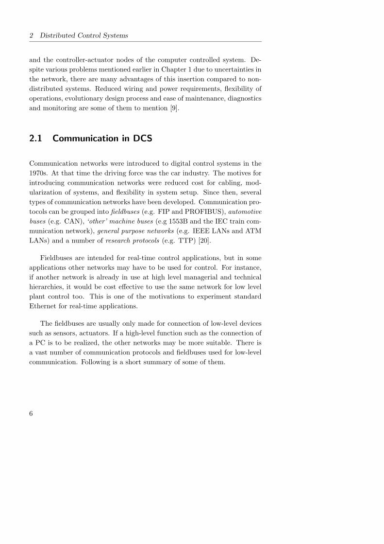
format [13]. Figures 2.2 and 2.3 show the respective frame formats, where
an introduction on each item in the frames is given next.
8
2.2 Ethernet
7
Preamble SFD DA SA FCS
Bytes 1 6 6 4
Type Data
46−15002
Figure 2.3: Ethernet frame
• Preamble - A 7 bytes pattern of alternating 1s and 0s used by the
receiver to establish bit synchronization.
• Start Frame Delimiter (SFD) - The bit sequence 10101011, which
indicates the actual start of the frame and enables the receiver to locate
the first bit of the rest of the frame.
• Destination Address (DA) - Specifies the station(s) for which the
frame is intended. It may be a unique physical address, a group address
or a global address
• Source Address (SA) - Specifies the station that sends the frame.
• Length - Length of LLC header and data field in bytes. (Only for
IEEE 802.3 frame)
• Type - Ethernet type field for identifying the contents of the data
field. (This field is included in the LLC header for IEEE 802.3.)
• LLC header - Logical Link Control header, i.e. IEEE 802.2 protocol.
• Data - The data to send is usually an IP datagram. This field has a
minimum size and has to be padded if it is shorter.
• Frame Check Sequence (FCS) - A 32 bit cyclic redundancy check,
based on all fields except Preamble, SFD and FCS.
The length of both frames, excluding Preamble and SFD, is between 64
and 1518 bytes. The minimum length of a frame is 64 bytes. Inter Frame
Gap (IFG) is the minimum time between two frames and this time depends
on the transmission speed. For a 10 Mbps LAN it is 9.6 µs and for a 100
Mbps LAN it is 0.96 µs as it is defined as multiples of 96 bits.
9
2 Distributed Control Systems
2.2.1 Ethernet model
OSI reference model
The Open System Interconnection (OSI) reference model was developed by
the International Organization for Standardization (ISO). The final stan-
dard, ISO 7498, was published in 1984. The model consists of seven layers
and these layers are described briefly in the following [14], [15]:
• Application layer - Provides access to the OSI environment for users
and also provides distributed information services.
• Presentation layer - Provides independence to the application pro-
cesses from differences in data representation.
• Session layer - Provides the control structure for communication be-
tween applications. It establishes, manages, and terminates connec-
tions between cooperating applications.
• Transport layer - Provides reliable and transparent transfer of data
between end points. Further it provides end to end error recovery and
flow control.
• Network layer - Provides the upper layers with independence from
the data transmission and switching technologies used to connect the
systems. Also it is responsible for establishing, maintaining, and ter-
minating connections.
• Data link layer - Provides the reliable transfer of information across
the physical link, sends frames with the necessary synchronization,
error control and flow control.
• Physical layer - Concerned with the transmission of unstructured
bit streams over physical media. It deals with the mechanical, elec-
trical, functional, and procedural characteristics to access the physical
medium.
10

2.2 Ethernet
The layers are usually referred with numbers, starting from the physical
layer as layer one. Every layer encapsulates the data in a protocol. The
encapsulation is usually done by adding a header to the data. In the data
link layer, the header covers the tail of the data as well. The physical layer is
slightly different, the protocol instead specifies a set of rules on the physical
interface with the following specifications;
• Mechanical: Specifies the pluggable connectors, signal conductors
and the wiring scheme.
• Electrical: Specifies the representation of bit values and transmission
rates.
• Functional: Specifies the functions performed between the physical
interface and the transmission media.
• Procedural: Specifies the sequence of events by which bit streams are
exchanged across the physical medium.
TCP/IP protocol suite
The TCP/IP protocol suite is a result of protocol research and development
conducted on the experimental network, ARPANET, funded by the Defense
Advanced Research Project Agency (DARPA), USA. The work started in
the late 1960s and has become the most widely used protocol suite for net-
work communication. There is no official TCP/IP protocol model, as in the
case of OSI. However, based on the protocol standards that have been devel-
oped, it is possible to organize the communication tasks into five relatively
independent layers as follows:
• Application layer - Provides communication between processes or
applications on separate hosts. File Transfer Protocol (FTP), Hyper
Text Transfer Protocol (HTTP) and Telnet are among the main pro-
tocols used here.
11

2 Distributed Control Systems
• Transport layer - Provides end to end data transfer service. This
layer may include reliability mechanisms. It hides the details of the
underlying network or networks from the application layer. The main
protocols used are Transmission Control Protocol (TCP) and User
Datagram Protocol (UDP).
• Internet layer - Concerned with the routing of data from the source
host to the destination host on one or more networks connected by
routers. The protocol used here is called Internet Protocol (IP).
• Network access layer - Concerned with the logical interface between
the end system host and the network. Carrier Sense Multiple Access
with Collision Detection (CSMA/CD) is the Media Access Protocol
(MAC) used.
• Physical layer - Defines the characteristics of the transmission
medium, the signaling rate and the signal encoding scheme.
A comparison of the OSI reference model with the TCP/IP model is shown
in Figure 2.4.
2.2.2 CSMA/CD access control
The devices communicate in half-duplex, when using Carrier Sense Multiple
Access with Collision Detection. The CSMA/CD is an improvement of the
CSMA access control technique [13]. The difference is that in CSMA/CD,
the station continues to listen to the medium while transmitting. This leads
to the following rules for CSMA/CD:
1. If the medium is idle, start to transmit, otherwise go to Step 2.
2. If the medium is busy, continue listening until the channel is idle, then
start to transmit immediately.
12

2.2 Ethernet
Application
Application
Presentation
Session
Transport
Network
Data link
Physical
Transport
Internet
Network Access
Physical
TCP / IP modelOSI model
Figure 2.4: OSI reference model vs TCP/IP model
3. If a collision among nodes is detected during transmission, transmit a
brief jamming signal to assure that all stations know that there has
been a collision and therefore to cease transmission.
4. After transmitting the jamming signal, wait for a random time slot
and then attempt to transmit again.
The segment length of the network has a maximum value to ensure that
all devices detect a collision. The IEEE 802.3 protocol standard specifies
this value for different physical layer media. Hence CSMA/CD gives rise to
time delays, which are non-deterministic, in the Ethernet network.
2.2.3 Half-duplex
For a Ethernet network with shared medium, the nodes must use the
CSMA/CD access control. This means that only one node is allowed to
13

2 Distributed Control Systems
transmit at a time. Examples of network topologies that have shared medium
are the bus topology, and the star topology interconnected with a hub [14].
2.2.4 Full-duplex
This includes a network with star topology interconnected with an Ethernet
Switch. Full-duplex means that transmission can be made simultaneously
in both directions. This also means that the sending node does not have to
sense that the medium is idle before transmitting. Hence the media access
delay can be avoided.
IEEE 802.3 defines a flow control for full-duplex Ethernet, namely the
media access control (MAC) PAUSE. When a receiving device detects an
upcoming buffer overflow, it will transmit a PAUSE control frame to the
sender, requesting it to stop transmission for a certain period of time. The
time is expressed as a multiple of 512 bit-times, which for a 10 Mbps LAN
is equal to 51.2µs, for a 100 Mbps LAN is equal to 5.12µs and so on. If
sufficient buffers will become free in the meantime, the receiver can re-admit
transmission by sending a PAUSE control frame with the pause duration
parameter zero to the sender. Usually the PAUSE control frames are used
to turn transmission on and off, because it is difficult to calculate an appro-
priate PAUSE timeout. The PAUSE control frame is not forwarded through
Ethernet Switches.
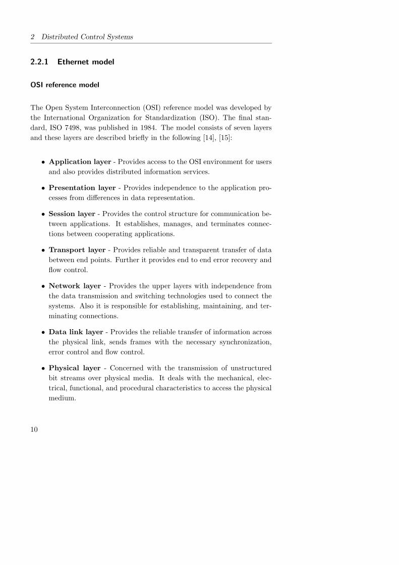
2.2.5 Ethernet Switch
An Ethernet Switch is a versatile hardware device to partition the available
network bandwidth into dedicated pieces without infringing the communi-
cation ability of the devices connected to it. Hence it allows full-duplex
communication without collisions. Forwarding decisions are made on the
Datalink layer of the OSI model as shown in Figure 2.5. The address learn-
ing function is usually updated automatically. Unlike the hub, the switch
14
2.2 Ethernet
Application
Presentation
Session
Transport
Network
Data link
Physical Data packet
Data packet Data packet
Data packet
Data packet
Application
Presentation
Session
Transport
Network
Data link
Physical
Physical medium
MACLLC
Physical medium
Host A Host B
Ethernet Switch
Figure 2.5: Ethernet Switch packet forwarding Host A to Host B based on
the Data link layer: Physical address
forwards the incoming frames only to the desired destination unless the frame
is a broadcast or a one with a non-existing destination address [14].
There are two basic transmission methods:
• Cut through - Switch starts sending packets as soon as they enter it
and their destination address is read within the first 20-30 bytes of the
frame. Thus the packets are forwarded to the destination, before they
are received completely. This reduces transmission latency between
ports, but it can propagate bad packets.
• Store and forward - Buffers incoming packets in the switch memory
until they are fully received and a cyclic redundancy check (CRC) is run
[13]. The buffered memory adds latency to the processing time, which
is proportional to the frame size. The store and forward switching
reduces bad packets and collisions that can adversely effect the overall
15

2 Distributed Control Systems
performance of the segment. These switches must buffer the frame,
until its re-transmission is commenced. The common approaches are;
Input buffering - One buffer per input port.
Output buffering - One buffer per output port.
Internal buffering - One memory pool shared by all ports.
The third approach has currently become the most popular despite the price
due to its higher memory utilization. However, cheap switches may still use
output buffering. The switch can use one of the two transmission methods
or possibly a mixture of both. The advantages of a switch over a hub are;
• Every port on the switch has its own collision domain.
• Since a port of the switch operates in full-duplex, it can receive and
transmit simultaneously as two ports.
An Ethernet network formed by connecting the stations (hosts) through
Ethernet Switches is called a Switched Ethernet network. With remarkable
speeds like 10 Mbps, 100 Mbps or even 1000 Mbps, Ethernet is one of the
most widely used local area network (LAN) technologies. But it is not in-
tended for real-time communications. However, the large number of installed
Ethernet networks will make it attractive to use in DCSs with the real-time
communication capability. Because all the other means of communications
used in DCSs are commonly in need of dedicated hardware. As a result they
inherit incompatibility among different bus systems and demand a high cap-
ital cost. On the other hand there exist cheap single chip solutions that
integrate Ethernet and TCP/IP stack. Furthermore, this integration can be
extended straight away to Internet. With the TCP, it is possible to use all
the conventional protocols such as FTP, HTTP, Telnet etc. Ethernet already
supports future requirements in bandwidth. As everybody will be using the
same protocol set, the solution is universal and thus compatibility issues
will be less. Vendors will only have to support a single platform instead of
multiple fieldbuses. At the same time the capacity of existing fieldbuses are
reaching their limits. Therefore it is unlikely that they would full-fill the
16

2.3 Ethernet for real-time applications : A survey
future needs of bandwidth [10]. Therefore it is worth investigating Ethernet
for lower level real-time applications.
2.3 Ethernet for real-time applications : A survey
This section summarizes the state of the art of adapting Ethernet in real-time
applications. Real-time means not only the reliable communication but also
its punctuality. It is vital to distinguish hard real-time from soft real-time
as they are significantly different. In hard real-time systems, the messages
must be delivered in a predefined time (deadline). Otherwise the contents of
the message become useless and the end results would lead to disagreeable
consequences, e.g. a system leading to instability. On the other hand in
soft real-time systems, like in multimedia applications, the consequences of
a late or missing packet is rather small, for example a pause in the music or
a flicker in the picture. Some of the efforts made in the literature to promote
Ethernet in hard/soft real-time applications are summarized below.
2.3.1 RETHER
The most interesting aspect of RETHER is its unique capability of support-
ing real-time bandwidth reservation and guarantee over existing Ethernet
infrastructure without any hardware support or modification. The only
modification required is the replacement of Ethernet driver with a RETHER
driver on every machine in the network [16]. But there has been many practi-
cal deficiencies found in RETHER. Firstly it is difficult to expose RETHER’s
real-time connection abstraction to user level applications without modify-
ing the operating system of the host. Secondly, installation of RETHER
drivers on mass scale is an expensive proposition from a system adminis-
tration standpoint. Thirdly, the token passing mechanism implemented in
RETHER is less appealing to compete in todays Switched Ethernet LAN
environment. Therefore it is no longer considered as an effective solution.
17

2 Distributed Control Systems
1
2
34
5
6 Switch
Figure 2.6: Ethereal Switch
2.3.2 EtheReal
The goal of the EtheReal is to build a scalable real-time Ethernet switch
that supports bandwidth reservation and guarantee over a switched LAN
environment without any hardware or operating system modification. With
the comparatively low prices of Switches, a star topology as shown in Figure
2.6 becomes a more realistic alternative over a token-timed based solution
as RETHER [15]. The EtheReal switch also offers buffers, which are used
to make priority features available. The main idea of the proposal is to have
bandwidth guarantee support (mainly for multimedia) in a star-topology
Switched Ethernet network. Every node is connected to other nodes via a
switch, modified to support real-time traffic. A Real-Time Communication
Daemon (RTCD) has to be installed in each node to support real-time traffic
consisting only of software. A RTCD is software add-on for the operating
system which schedules the traffic. The significant feature of EtheReal over
the predefined bandwidth guarantee is its soft real-time traffic support with
priority scheduling. EtheReal supports non-real-time traffic as well [16].
18

2.3 Ethernet for real-time applications : A survey
Synchronization pulseTEMPRA Bridge
Figure 2.7: TEMPRA network
2.3.3 TEMPRA
This project focuses on how to implement time determinism in an Ethernet
network. This solution consists of nodes connected to a single bus, i.e.
a shared-medium topology. In one end of the bus, a TEMPRA bridge is
installed as shown in Figure 2.7 to schedule the network traffic. The idea
of the TEMPRA solution is based on a master-slave solution, where the
TEMPRA bridge at the end of the bus is the master. When the bus is idle,
the bridge transmits a synchronization pulse. Every node on the bus waits
for this synchronization pulse and a timeout starts when a node receives
this pulse. When the timeout reaches the expire limit, the node is allowed
to transmit on the medium. Setting the timeout sets the priority of the
respective node. For instance a lower timeout means a higher priority. This
eliminates collisions in the underlying Ethernet network. But this solution
requires a hardware reconfigured Ethernet card that supports TEMPRA
protocol. Furthermore, modifications in the host operating system are also
necessary.
2.3.4 SIRTE
Switched Industrial Real-Time Ethernet (SIRTE) is based on a 100 Mbps
Ethernet switch supporting hard real-time traffic with bandwidth and la-
tency guarantee, i.e. a predefined amount of data is delivered before a dead-
19

2 Distributed Control Systems
line. The guarantee is upheld by real-time channels, which can be created
and closed dynamically. The nodes, which are connected to the switch, can
either be real-time nodes or non real-time nodes depending on which quality
of service (QoS) level is required. Nodes with no SIRTE drivers installed
are non real-time. In the proposed solution there are no modifications of the
Ethernet hardware on the network interface cards. The real-time communi-
cation support in the nodes and the switch are handled by a software added
between the Network layer and the Data link layer (Middle-ware), in the
OSI reference model. However, some additional hardware to the standard
Ethernet switch are needed. The switch has the overall responsibility for es-
tablishing, maintaining and terminating different node connections through
it. The software in the end nodes includes the application program interface
(API) and the simple regulations of the traffic passing through the protocol
suite. The product is not yet commercially available [17].
2.3.5 IPv6
IPv6 or Internet Protocol version 6, was recommended by the Internet En-
gineering Task Force (IETF) in 1994 for the Internet layer of the TCP/IP
protocol suite. In 1998, the core set of IPv6 protocols became an IETF
drafted standard. IPv6 is a new version of IP that is designed to be an evo-
lutionary step from IPv4, the current version. It is supposed to fix several
problems now being encountered with IPv4 in the context of DCSs, such as
auto-configuration and support for real-time traffic. In addition, the revised
IP header with 128 bits address field gives an unlimited number of global
addresses [18]. The most significant features are further described below.
Auto-configuration
In IPv4, the network addresses need to be set-up manually or by using Dy-
namic Host Configuration Protocol (DHCP). In contrast, IPv6 allows auto-
configuration of addresses, thus the network management is greatly simpli-
fied. The self-generated IPv6 address combines a local network identifier
20

2.3 Ethernet for real-time applications : A survey
and an identifier generated by the node in the “plug-and-play” fashion. By
simplifying the maintenance of large networks of simple devices, such as sen-
sors and actuators of DCSs, this automated procedure paves the way for the
large scale introduction of Ethernet technology into industrial environments.
Support for real-time traffic
The IPv6 header contains two fields specifically targeted at real-time appli-
cations, the “Traffic Class” and the “Flow Label”. The Traffic Class is an
8-bit field that enables switches to distinguish real-time packets from non-
real-time packets. The Flow Label is a 20-bit label identifying flows. The
IPv6 specification describes a flow as a sequence of packets sent from a par-
ticular source to a particular destination. This will be an important feature
for the DCSs in defining application specific sensor/actuator and controller
nodes.
Performance
Performance comparison presented in [19] reveals that IPv4 is slightly faster
than IPv6 on a very simple back to back connected network with software
implemented TCP/IP stacks. The reason pointed out is the fact that the
IPv6 solution is a recent product, where as the IPv4 stack has undergone
a number of performance enhancements over the past 20 years. When the
network is expanded by adding a router, again IPv6 becomes much slower.
Still IPv6 can not be rejected completely as the current networking hardware
is not optimized for IPv4. Thus no complete conclusions can be drawn on
the performance until tests are conducted on hardware optimized for IPv6.
21

2 Distributed Control Systems
22

3 Problem Formulation
This chapter starts off with a component description of the DCS to be used
in the report. It is then extended to establish the complete DCS followed by
an onion layer task analysis. Obtaining the system model together with the
desired performance criteria is also presented. The test rig mainly consists
of a Brushless DC Motor, a local servo amplifier, an Ethernet network and
a software controller implemented in a PC. Figure 3.1 shows the physical
layout of the test rig and a short description of each item follows.
3.1 Brushless DC motor
The Brushless DC motor considered is a 0.4 kW, 4000 rpm, non-salient
permanent magnet (PM) synchronous machine with trapezoidal flux distri-
bution in the air gap due to concentrated full pitch windings in the stator.
These motors are becoming increasingly attractive in servo and variable
speed applications due to their high torque to inertia ratio and long term
maintenance free operation due to the absence of brushes and mechanical
commutation [11]. The dynamical equations of the motor derived in [12] can
be given as
Van
Vbn
Vcn
=
Rs 0 0
0 Rs 0
0 0 Rs
iaibic
+d
dt
L M M
M L M
M M L
iaibic
+
eaebec
.
(3.1)
23

3 Problem Formulation
Iref Idω ref
ω r
sR
sReaeb
ec
sR
ia
ib
ic
ω r
CurrentSignals
Iref
SpeedSignals
ADC
DAC
Network Interface
f/V
ControllerSpeed
Network Interface
Vdc a b cL
L
L
Local Servo Amplifier
BLDC motor
Ethernet LAN
Micro−Controller
PWM signals
PWM signals
Decoder
X
+
−
Figure 3.1: Block diagram of the test rig
Due to symmetry in the isolated neutral configuration of the stator winding,
ia + ib + ic = 0. (3.2)
Hence
Mib +Mic = −Mia. (3.3)
Substituting equations (3.2) and (3.3) into equation (3.1) results in,
diadtdibdtdicdt
=
−Rs
Ls0 0
0 −Rs
Ls0
0 0 −Rs
Ls
iaibic
+
1Ls
0 0
0 1Ls
0
0 0 1Ls
Van
Vbn
Vcn
−
eaLsebLsecLs
,
(3.4)
where
Ls = L−M.
24

3.2 Local servo amplifier
The electromagnetic torque generated is
Te =
[
P
2
]
eaia + ebib + ecicωe
. (3.5)
The mechanical torque equation is
Te − TL = J
[
2
P
]
dωe
dt+Bf
[
2
P
]
ωe. (3.6)
ωe =
[
P
2
]
ωr (3.7)
Hence this is simply an AC motor working as a DC motor [12]. The motor
is loaded by a shaft that is coupled to an identical motor working as a
generator.
3.2 Local servo amplifier
This module mainly comprises the analog current controller and the
MOSFET driven inverter acting as the electronic commutator. In the torque
mode, the current reference signal Iref is the external command input to the
closed loop system formed by the decoder, the hysteresis comparator and
the PWM generator. There are three “Hall sensors” placed on the stator
of the BLDC motor that give 120(electrical) phase shifted square waves in
phase with respective phase voltages. These waves represent the stator cur-
rents. The decoder circuit converts the latter waves into the six-step signals
as shown in Figure 3.1. These converted signals with appropriate polarities
are then used to drive the gates of the MOSFETs of the respective phases.
The actual phase currents of the motor track the command currents with a
hysteresis current controller. In BLDC motors, only two of the phase cur-
rents are enabled at any instant, one with positive polarity and the other
with negative polarity. This makes the currents of adjacent phases equal in
magnitude but opposite in direction. When these currents (equal in magni-
tude) tend to exceed the hysteresis band, both the respective MOSFETs are
turned off at that same instant to initiate current feedback through the free
wheeling diodes. The rotor position is determined by a shaft encoder and
the speed is calculated by differentiating the rotor angle [23].
25

3 Problem Formulation
3.3 Controller
The speed controller is implemented digitally in a PC using GNU C++
running on Red Hat Linux 7.2 platform. In addition to producing reference
signal Iref to the current controller in the local servo amplifier, the controller
has to compensate for the network induced delays.
3.4 Network
The network bridges the speed controller and the motor drive forming the
distributed control system, but at the price of network induced delays. The
PC is interfaced to the network through its normal 10/100 Mbps network
interface card (NIC). The motor side is interfaced to the network through
Ethernet connectible Z-World BL2100 Micro-Controller at 10 Mbps, pro-
grammed using Dynamic C Premier 7.02 [21]. Its interface to the Local servo
amplifier is through 16 bit analog to digital converters (ADC) and +10 V to
-10 V digital to analog converters (DAC) [22]. Standard connection oriented
TCP sockets are used to connect through the network. Therefore in addi-
tion to Iref and ωr, synchronizing and acknowledgment signals are sent back
and forth at the establishment, data transfer and termination phases of the
TCP connection. Ethernet frame size is fixed at 64 bytes when defining the
sockets. The physical arrangement of the entire test rig is shown in Figure
3.2.
3.5 Time delayed system
3.5.1 Overview
To simplify the analysis, the entire system can be viewed in an onion layout
[27]. These layers are
26

3.5 Time delayed system
Figure 3.2: BLDC motor drive controlled via Ethernet
1. layer 2 - Micro-controller triggering the tasks of the sensor, actuator
and their interface to the network.
2. layer 1 - Network to map the speed data from the sensor to the con-
troller and the control signal from the controller to the actuator.
3. layer 0 - PC interfaced to the network, which calculates the control
signal.
Thus each layer has several tasks to carry out, where each of them has a
deadline in reaching real-time performance of the DCS. To produce a stable
output, they must be arranged in a chronological order. The first digit of
the task subscript corresponds to the layer number, while the second is for
the task. In layer 0, the logical order of the tasks are:
27

3 Problem Formulation
• t00 - extract speed data from the received TCP packet.
• t01 - calculate the control signal.
• t02 - encapsulate the control signal into the TCP packet to be sent.
They may be clock-triggered (time-triggered) or event-triggered. When
clock-triggered, the start of task t00 is synchronized with the internal clock
of the PC and the start of t01 and t02 will depend on the release time and
the scheduling algorithm used. On the other hand, in event-triggered layer
0, t00 waits until the arrival of the first speed data to start off and t01 and
t02 are executed sequentially. At the end of t02, t00 again starts waiting for
the next speed data and this procedure repeats. Therefore whether it is
clock triggered or event triggered, the total task execution time of layer 0 is
approximately constant.
The tasks of layer 1 are
• t10 - map speed data from sensor to controller.
• t11 - map control signal from controller to actuator.
In layer 1, time for mapping is influenced by the network topology, the
nominal bandwidth, the available bandwidth, the number of active nodes
and the distance between nodes etc. Hence the exact completion time of
layer 1 is non-deterministic a priori.
The layer 1 considered here is implemented in the standard 10 Mbps
Ethernet network. If it is to be clock triggered, it has to be synchronized
with the clocks of layer 0, layer 2 or both. The analysis and implementation
become less complicated if layer 1 is also to be event triggered.
In layer 2, the logical order of tasks are
• t20 - sampling the speed.
28

3.5 Time delayed system
• t21 - analog to digital conversion.
• t22 - encapsulate the speed data into a TCP packet to be sent.
• t23 - extracting the control signal from the received TCP packet.
• t24 - digital to analog convert the control signal.
• t25 - release the analog control signal to the actuator.
In order to define an exact starting point for the distributed control loop,
task t20 is made time triggered. It also simplifies the analysis as there is
going to be a unique and constant sampling interval for the entire DCS. The
rest of the tasks are made event triggered. Hence only t20 is time triggered
and periodic and the others are event triggered and non-periodic. Since
the execution time of the tasks t10 and t11 depends on the instantaneous
network condition, the total worst case execution time (WCET)s are non-
deterministic.
The problem here is to design a speed controller to be implemented in
layer 0, to ascertain closed loop operation of the BLDC motor despite the
non-determinism in t10 and t11. The shorter the control delay τ i.e., time
from sampling interval to the time where the corresponding control signal
is released to the actuator, the closer the distributed system approaches the
non-networked closed loop system.
3.5.2 Open loop model
It is important to have a linear model of the system in order to design a
suitable speed controller. As in the conventional control system terminology,
the ‘plant’ is everything else other than the network and the controller, i.e.,
the BLDC motor and the local servo amplifier.
There are two possibilities in modeling the plant. One way is to model
each component individually and cascade them to obtain the complete plant.
The other method, which is less prone to accumulated model errors, is to
29

3 Problem Formulation
build an input - output model. The entire plant is considered as a single
model by means of some system identification experiments. This can be done
by observing the response of the overall open loop plant to a known input
signal and fitting the system model of suitable order to the recorded input -
output behavior. The advantage here is the possibility of obtaining a simple
model, which depends only on the dominant modes of the overall system.
One disadvantage is the possibility of some non-linear behaviors contained
in the system affecting the linear input-output relationship. Nevertheless,
since the requirement is to come up with a simple linear model, the second
method is used.
In order to obtain a linear model, the plant must operate in the linear
region of its performance range. As stated in [30], the linear operation of a
BLDC motor is badly affected by its inherent cogging torque specially at low
speeds. In order to identify the linear operating region in practice, first a slow
sinusoidal input of typically 1.0 Hz frequency and a reasonable amplitude is
applied to Iref with the speed control loop open. By gradually increasing
the amplitude of the input sinusoidal waveform, the saturation limits of
the plant can be identified when the distortions are visible in the response.
The linear operating region of the motor drive and the corresponding input
signal range that will keep the system within the linear region can then be
identified, from this basic experiment. The next step is to apply a standard
input signal to the system and record the output. To do this, a constant
voltage greater than the lower threshold is applied and at steady state, a step
with an upper bound below the identified saturation limit is superimposed.
The corresponding speed response is in the linear operating region. This
speed response is approximated using curve-fit functions of MATLABTM to
derive the transfer function of the open loop plant. Preliminary investiga-
tions on the recorded input-output data reveal that the first order model of
the form k/(s+ a) fits to the data satisfactorily.
30
3.5 Time delayed system
0 0.2 0.4 0.6 0.8 1 1.2 1.4 1.6 1.8 21.4
1.6
1.8
2
2.2
2.4
I ref
0 0.2 0.4 0.6 0.8 1 1.2 1.4 1.6 1.8 20.2
0.4
0.6
0.8
1
Spee
d re
spon
se
time (s)
Model SpeedMotor Speed
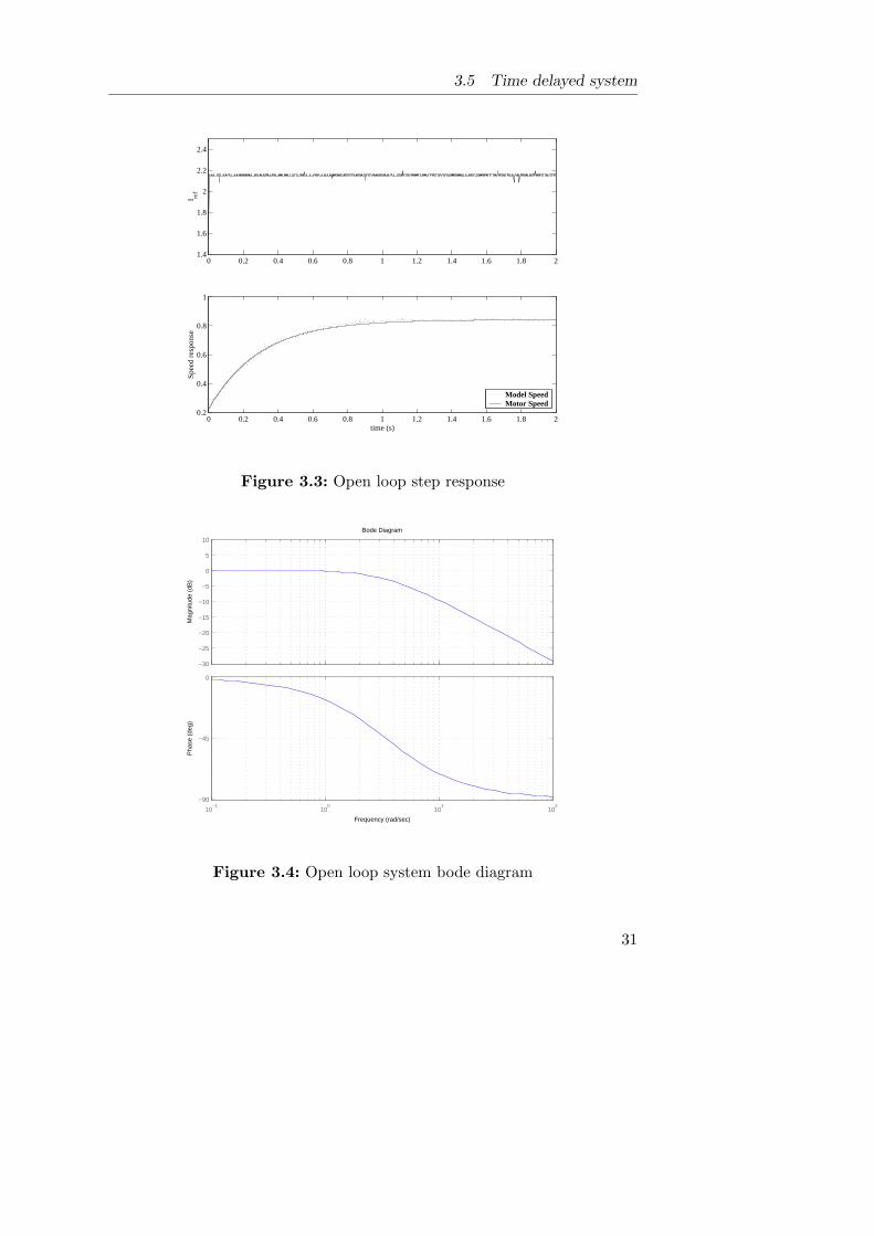
Figure 3.3: Open loop step response
Bode Diagram
Frequency (rad/sec)
Pha
se (
deg)
Mag
nitu
de (
dB)
−30
−25
−20
−15
−10
−5
0
5
10
10−1
100
101
102
−90
−45
0
Figure 3.4: Open loop system bode diagram
31

3 Problem Formulation
3.5.3 Design criteria
In the open loop step response shown in Figure 3.3, it can be seen that the
rise time is nearly 1 s and is aimed to bring it down to 0.1 s at minimum
overshoot. Since the rule of thumb [24] is to have 4 to 10 samples per rise
time, the sampling time h is taken as 10 ms constant. The system bandwidth
usage is therefore approximately 0.1 Mbps.
32
4 Analysis of time delayed systems
In this chapter, a timing analysis is carried out on a general DCS. A first
order system similar to the plant in Chapter 3 is used to demonstrate the
effects of time delays on the distributed closed loop operation.
4.1 Timing Analysis
In the timing analysis, the tasks to be considered are (i) sampling the sensed
plant output, (ii) calculating the control signal by executing the control algo-
rithm, (iii) feeding the actuator with the control signal and (iv) implementing
the inter-node communication. These tasks can be split into more detailed
activities that affect, with different degrees of strictness, to the system timing
behavior and its performance.
It is important to stress that strictness in timing behavior of control sys-
tems usually means that actions must be started at exact time instants. In
hard real-time systems, strictness additionally implies that worst case exe-
cution time (WECT)s of tasks must be less than or equal to their respective
deadlines. In both cases, a common fact is that missing an action on time
will result in an unacceptable output.
Moreover, it has to be pointed out that the control theory and the
practice can follow many paradigms such as continuous or discrete control;
centralized or distributed control; direct, feedback or feed-forward control;
mono-rate or multi-rate control; classical, adaptive or fuzzy control. One or
33

4 Analysis of time delayed systems
τsccaτ
cτ
Plant
Reference
NetworkNetwork
ActuatorContinuous Time
Discrete Time
h
Sampler
Controller+ jitter
Figure 4.1: Distributed Control System (DCS)
many of these paradigms are found in any control system, implying different
timing behaviors.
Therefore, time is an important issue in control systems, when timing
behavior, schedulability, performance and quality of service (QoS) issues
are concerned. Control theory assumes a highly deterministic timing of the
implementation, as described in [24]. Consequently, [25], [26] and [27] have
treated deficiencies in the computer system implementation of the DCS with
respect to time-variations and time-restrictions.
Figure 4.1 outlines which timing specifications that should be derived
from DCSs in order to understand the significant timing behaviors of a com-
puter controlled distributed feedback control systems.
Beside the network, it consists of the three main nodes; the controller
node with an embedded reference signal generator, the sampler node and
the actuator node. In the typical control scenario as per the onion model
analysis in Chapter 3, the following functionality is expected when all tasks
34

4.1 Timing Analysis
jitter toltol tolsample sampleactuateτ τ τsc c ca
kh (k+1)h
releaseTTstart
Tcomplete
Figure 4.2: Timing data of a DCS
but sampling are non-periodic: When the sampler operates on the plant
output with a fixed period h, the global time for the nth sampling instant is
given by
tsample (n) = tsample (n− 1) + h. (4.1)
When the sampler has collected the data, it is mapped to the controller,
introducing a communication delay τsc. The controller starts execution cor-
responding to the nth sample at
tcontrol (n) = tsample (n) + τsc. (4.2)
The controller executes the control algorithm in order to derive the ac-
tuating signal, introducing a computing delay τc. The controller maps the
actuating signal to the actuator, introducing another communication delay
τca. Finally the actuator performs actuation at the time given by
tactuate (n) = tcontrol (n) + τc + τca. (4.3)
In this short description, it is shown that every-time the control algorithm
is executed, a computing delay τc is introduced. It is assumed that the
sampler and the actuator operate virtually in zero time. In order to be more
realistic, it is necessary to introduce an acceptable deviation (tolerance) from
the instant of the sampling (tolsample), and a similar tolerance for actuation
(tolactuate) (Figure 4.2). Then equations (4.1) and (4.2) can be modified to
tsample (n) = tsample (n− 1) + h± tolsample (4.4)
35

4 Analysis of time delayed systems
tactuate (n) = tcontrol (n) + τc + τca ± tolactuate. (4.5)
Moreover, the controller timing analysis could be made more precise if the
release time Trelease, start time Tstart, jitter (varying or fixed difference be-
tween Trelease and Tstart) and the completion time Tcomplete of the controller
activity are introduced. Then equation (4.2) becomes
tcontrol (n) = tsample (n) + τsc + jitter. (4.6)
Thus the distributed control system has two inter-task communication pro-
cedures that introduce delays (fixed or varying) in the timing behavior. Fi-
nally, the the total execution time, from the sampling to the actuation of
the control system, termed as the control delay, can be given by
τ (n) = tactuate (n)− tsample (n) . (4.7)
4.1.1 Discrete Time Control System
In this section, the mathematical description of a general control system
is derived and is extended to a system with input time delays. The total
control delay τ derived in equation (4.7) has been used for the analysis. A
general control system in continuous time can be derived as
dx(t)
dt= Ax (t) +Bu (t) (4.8)
y (t) = Cx (t) .
Discretizing the system (4.8) at a sampling interval h, gives
x (kh+ h) = Φ (h)x (kh) + Γ (h)u (kh) (4.9)
y (kh) = Cx (kh) ,
where
Φ (h) = eAh (4.10)
Γ (h) =
∫ h
0eAs dsB. (4.11)
36

4.1 Timing Analysis
The discrete transfer function between input and output can be derived as
Y (z)
U (z)= C [zI − Φ (h)]−1 Γ (h) . (4.12)
The system equations derived above assume negligible τ compared to h. It
is true as long as the system is non-distributed i.e., centralized systems.
But practically all the contributors to τ i.e., τsc, τc, τca and jitter can have
significant magnitudes compared to h. Therefore, τ = τsc + τc + τca + jitter
as derived in equations (4.1) to (4.7), become comparable with h when the
system is distributed through a temporal constrained media mentioned in
Chapter 2. In such a case, the system in equation (4.8) has to be modified
as
dx(t)
dt= Ax (t) +Bu (t− τ) (4.13)
y (t) = Cx (t) .
For 0 < τ < h, the discretized version of equation (4.13) becomes
x (kh+ h) = Φ (h)x (kh) + Γ0 (h,τ)u (kh)
+ Γ1 (h,τ)u (kh− h) (4.14)
y (kh) = Cx (kh) , (4.15)
where
Φ (h) = eAh
Γ0 (h,τ) =
∫ h−τ
0eAs dsB (4.16)
Γ1 (h,τ) = eA(h−τ)
∫ τ
0eAs dsB. (4.17)
The new transfer function is
Y (z)
U (z)= Cz−1 [zI − Φ (kh)]−1 [zΓ0 (h,τ) + Γ1 (h,τ)] . (4.18)
37

4 Analysis of time delayed systems
4.1.2 Effect of time delays
Model equations (4.13) to (4.17) remain valid for constant τ as well as vari-
able τ as long as 0 < τ < h. Compared to the non-distributed transfer
function in equation (4.9) the distributed system in equation (4.17) has an
additional zero at −Γ1(h,τ)/Γ0(h,τ) and a pole at the origin of the z-plane,
caused by the delay. For h < τ , introducing τ = (d− 1)h+ τ′simplifies the
computation, where 0 < τ′< h and d is an integer. Then equation (4.14)
has to be changed as
x (kh+ h) = Φ (h)x (kh) + Γ0
(
h,τ′)
u (kh− dh+ h)
+ Γ1
(
h,τ′)
u (kh− dh)
y (kh) = Cx (kh) . (4.19)
The new discrete transfer function becomes
Y (z)
U (z)= Cz−d [zI − Φ (h)]−1
[
zΓ0
(
h,τ′)
+ Γ1
(
h,τ′)]
. (4.20)
For this case too, the model equations are valid even for variable τ as long
as d remains constant to a given system and τ′can vary in 0 < τ
′< h.
Change of d from cycle to cycle depending on the subsequent control delay,
results in a respective change in the order of the closed loop system. This
can further be exemplified if numerical values are substituted for d. Starting
from the most trivial case with d = 1, i.e., for 0 < τ < h, the state space
model is[
x (kh+ h)
u (kh)
]
=
[
Φ Γ1
0 0
][
x (kh)
u (kh− h)
]
+
[
Γ0
I
]
u (kh) . (4.21)
Next for d = 2 i.e., for h < τ < 2h, the state space model is
x (kh+ h)
u (kh− h)
u (kh)
=
Φ Γ1 0
0 0 0
0 0 I
x (kh)
u (kh− 2h)
u (kh)
+
Γ0
I
0
u (kh− h) .
(4.22)
38

4.1 Timing Analysis
Further for d = 3 i.e., for 2h < τ < 3h, the state space model is
x (kh+ h)
u (kh− 2h)
u (kh− h)
u (kh)
=
Φ Γ1 0 0
0 0 0 0
0 0 I 0
0 0 0 I
x (kh)
u (kh− 3h)
u (kh− h)
u (kh)
+
Γ0
I
0
0
u (kh− h) .
(4.23)
Hence the system matrix gets the dimension (d + 1) × (d + 1). Therefore it
is obvious that for a given system d must remain constant from cycle to
cycle for the order of the system matrix to be constant and hence the model
to be valid. In practical terms, variations of control delay, only within two
successive multiples of sampling interval are acceptable.
From the transfer function in equation (4.20), it can be seen that the
larger the values of d i.e., the delay compared to the sampling interval h,
the higher the number of poles added at the origin. Hence the controller
should be able to cancel them in order to maintain the system stability. The
additional zero only affects the transients but not the stability. Since Γ0 > 0
and Γ1 > 0, the zero is from 0 to -1 in the z - plane and therefore the effect
of the additional zero on transients is negligible [27].
4.1.3 Simulation results
A first order system, which is the case for most practical motion control
systems as well as the test-rig in this report, is chosen to illustrate the
effect of control delay on stability and the transient behavior on the DCS.
Substituting to equations (4.10), (4.11) and (4.17) gives
x (kh+ h) = e−ahx (kh) +k
a
[
1− e−ah]
u (kh) (4.24)
y (kh) = x (kh) ,
39

4 Analysis of time delayed systems
for the system G(s) = k(s+a) at τ = 0, where A = [−a], B = [k] and C = 1
in continuous time. In the distributed system,
Γ0 (h,τ) =k
a
[
1− e−a(h−τ)]
(4.25)
Γ1 (h,τ) =k
a
[
e−a(h−τ) − e−ah]
. (4.26)
Performance degradation when d increases was simulated and is shown in
Figure 4.3, where the speed loop is closed with a simple PI controller, de-
signed without considering the delay.
Accordingly, it can be seen that in order to nullify the performance
degradations (caused by distribution itself and its consequence i.e., the time
delays) and to maintain the performance as close as possible to the non-
distributed version of the control system, the controller must somehow can-
cel the cause of forming the additional poles and the zero. Further, the
degradation pattern shown is plant dependent, i.e., the type of deterioration
of the output response depends on the order of the system considered.
4.2 Controllability and Observability
Based on equations (4.21), (4.22) and (4.23), the system G, input H and
output C matrices in the state space form can be defined for different ranges
of τ according to the following sections.
1. For 0 < τ < h
G =
[
Φ Γ1
0 0
]
(4.27)
H =
[
Γ0
I
]
C =[
1 0]
40

4.2 Controllability and Observability
0 0.5 1 1.5 2 2.5 3 3.5 4 4.5 50
0.2
0.4
0.6
0.8
1
1.2
1.4
time (s)
Spee
d re
spon
se
No delayd=1d=2d=3d=4
Figure 4.3: Step response variation with d
rank[
H... GH
]
= 2 (4.28)
rank[
G′... G′C ′
]
= 2 (4.29)
As the rank of equations (4.28) and (4.29) are the same as the order
of G, the system is both controllable and observable [28].
41

4 Analysis of time delayed systems
2. For h < τ < 2h
G =
Φ Γ1 0
0 0 0
0 0 I
(4.30)
H =
Γ0
I
0
C =[
1 0 0]
rank[
H... GH
... G2H
]
= 2 (4.31)
rank[
G′... G′C ′
... G′2C ′
]
= 2 (4.32)
As the rank of equations (4.31) and (4.32) are one less than the or-
der of the system matrix, the system looses both controllability and
observability by one degree.
3. For 2h < τ < 3h
G =
Φ Γ1 0 0
0 0 0 0
0 0 I 0
0 0 0 I
(4.33)
H =
Γ0
I
0
0
C =[
1 0 0 0]
rank[
H... GH
... G2H... G3H
]
= 2 (4.34)
rank[
G′... G′C ′
... G′2C ′... G′3C ′
]
= 2 (4.35)
42

4.3 Delay model
Similar to the previous case, as the rank of equations (4.34) and (4.35)
are two less than the order of the system matrix, the system looses both
controllability and observability by two degrees.
This suggests to keep the order of the system matrix unchanged, irre-
spective of the delay. The only possibility of doing so is to use past control
inputs and delayed measurements of state variables and their timing data in
estimating the actual state of the plant by the time that the control signal
is applied to the actuator. Hence the system order and then the control-
lability and observability can be maintained as in the case of non-delayed
system. This is the basis for the state feedback controller design presented
in Chapter 5.
4.3 Delay model
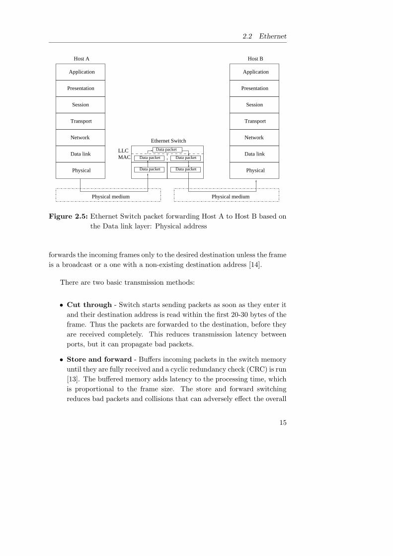
Figure 4.4 shows the statistics of the variation of the control delay τ . It
clearly shows that both under high and low network traffic, the control
delay is not exactly constant. It varies stochastically about a mean value in
a network status dependent manner.
In PI and Smith Predictor speed controller structures, the control delay
τ will be treated as a constant equal to its mean value τmean. As a function
in the Laplace domain, it will appear as e−τmeans. To bring it to the pole-zero
based transfer function format, Pade′ approximation can be used [29]. In
the state feedback controller, real-time control delay τk is used.
43

4 Analysis of time delayed systems
8.5 9 9.5 10 10.5 110
200
400
600
800
1000
1200
1400
τk (ms)
(a)
Num
ber
of o
ccur
ence
s τmean
= 9.29 ms
15 15.5 16 16.5 17 17.5 180
200
400
600
800
1000
1200
1400
τk (ms)
(b)
Num
ber
of o
ccur
ence
s τmean
= 16.16 ms
Figure 4.4: Control delay variation.
(a) Low network traffic; (b) High network traffic.
44

5 Controller design for the time
delayed system
In sections 5.1 and 5.2 of this chapter, the standard controller structures
Proportional Integral (PI) and Smith predictor will be summarized in the
way they were implemented on the test rig in practice. Section 5.3 presents
the state feedback controller with on-line delay compensation, which is an
original contribution.
5.1 PI controller
This method is applicable only for the case where 0 < τ < h. In other
words, it must be guaranteed that the samples arrive at the controller node
in chronological order. Then the damage caused by the delay is limited to
the non-periodic arrival of the control signals at the actuator node. Since the
Proportional Integral (PI) controller derived here assumes a constant delay
in tunning its parameters Kp and Ki, at least the transient performance
will be degraded by a certain degree, when variations in τ are encountered.
Further, degradations can be expected when τ increases beyond h. The
tunning rules for the PI controller are first derived in [31] as
45

5 Controller design for the time delayed system
Kp =1
kτmean(5.1)
Ki =1
3kτ2mean
for a first order, type 1 time delayed system kse−τmeans. Later some
modifications are added by trial and error in [33] and [34] as
Kp =0.236a
k
[
1
aτmean
]0.959
(5.2)
Ki =0.111a2
k
[
1
aτmean
]1.698
for the first order, type 0 time delayed system, k(s+a)e
−τmeans. These
tunning rules are used in designing the PI controller for the test rig.
5.1.1 Discretization
The continuous time PI controller[
Kp +Ki
s
]
is discretized using the Bilinear
transformation s = 2h
[
z−1z+1
]
. The resulting discrete time controller mapping
the exact poles and zeros from the Laplace s-plane to the z-plane [32] is given
byU(z)
E(z)=KP −KIz
−1
1− z−1, (5.3)
where
KP = Kp +Kih
2, (5.4)
KI = Kp −Kih
2. (5.5)
46

5.1 PI controller
5.1.2 Integrator Wind-Up problem
In order to make sure the proper implementation of the PI controller designed
as specified before, some considerations must be given to certain hardware
limitations of the system. One such important limitation is the dynamic
operating range of the Digital to Analog Converter (DAC) of the actuator
node. This will impose both upper and lower limits for the control signal
computed from the PI controller. If the control signal exceeds these limits,
the derived control signal u(t) will no longer apply on the system as shown in
the Figure 5.1 and the expected output variation will slow down as a result.
This will make the integrator output to increase due to the non-zero error
that is fed into it for a longer duration. This is known as the integrator
wind-up and an elaborated description of this scenario can also be found
in [24] and [35]. Employing a suitable integrator anti-windup scheme in
the controller is always recommended for PI controller applications, which
improves the reliability of the control system.
One way to bring the integrator value down to the limits of the DAC is
to incorporate the tracking algorithm explained in [24] and [35]. This will
force u(t) to follow v(t). The discrete time PI controller incorporating the
tracking algorithm can be given as
uP (k) = KP e(k) (5.6)
u(k) = uP (k) + uI(k) (5.7)
uI(k + 1) = uI(k) +KIe(k) + v(k)− u(k) (5.8)
v(k) = sat[u(k)], (5.9)
where
sat[u] =
umin if u < umin
u if umin < u < umax
umax if u > umax.
Here umax and umin are the maximum and minimum hardware limitations
of the DAC respectively.
47

5 Controller design for the time delayed system
−1z
ω
ωref
(k)
e(k) u(k) v(k)
KAWC
KI
KP
−+
−
+
+
+
+
+(k)
+
+
Figure 5.1: Discrete time integrator anti-windup compensator
The integrator value can be forced back into the linear region by feeding
back a fraction of the difference between the controller output u(k) and the
saturated output v(k) as shown in Figure 5.1. The modified equation for
controller is implemented as
u(k) = KP e(k) +q−1
1− q−1[KIe(k) +KAWC(v(k)− u(k))]. (5.10)
5.1.3 Stability Problem
An integrator is marginally stable. At saturation when the integrator starts
acting freely, it can be made more stable by feeding back the term u(k) −
v(k). This is due to the fact that the pole of the integrator on the unit
circle in z-plane is shifted into the unit circle by means of KAWC . This
scenario of forming a more stable closed loop is illustrated in Figure 5.2.
The corresponding transfer function is given by
U(z)
V (z)=
KAWCz−1
[1− (1−KAWC)z−1]. (5.11)
48

5.2 Smith Predictor
KI
KAWC
KP
u(k) v(k)v(k)
u(k)
e(k)e(k)
−1z
−1z1−
+ ++ +
+
Integral part Proportional part
−
Figure 5.2: More stable closed loop by fine tunning KAWC
This clearly shows the movement of the integrator pole from 1 to (1 −
KAWC). This stable system always attempts to bring the controller output
u(k) equal to v(k). Hence, the dynamics of the system can be changed by
using KAWC as a tuning parameter [36]. In practice, a value for KAWC has
to be chosen by trial and error depending on the transient response required.
5.2 Smith Predictor
O. J. M. Smith proposed a controller structure shown in Figure 5.3 that is a
well known as an effective dead-time compensator for stable processes with
time-delays. And this controller is very much applicable for situations, where
τ > h. As far as the control delay variations (Figure 4.4) are concerned, its
adaptability to control of distributed systems is worth investigating. Be-
cause τ can grow large compared to h and the open loop time constant 1/a,
when the system undergoes heavy network traffic. The closed loop transfer
function of the complete distributed system in Figure 5.3 can be given by
ω(s)
ωref (s)=
Gc(s)G(s)e−τs
1 +Gc(s)[Gm(s) +G(s)eτs −Gm(s)eτmeans], (5.12)
where
49

5 Controller design for the time delayed system
ωref
cG (s) G(s) −τe
s
−τest seGm(s)
+ +
+
−
−
ω(s)(s)Actual motor with network
Model motor with network
−
Figure 5.3: Nominal Smith predictor architecture
G(s) is the plant to be controlled,
Gest(s) is the estimated system model of G(s),
Gc(s) is the controller,
τest is the estimated control delay.
Stability of the Smith predictor is affected by the accuracy with which the
model i.e., Gest(s) and τest represent G(s) and τ respectively. In the open
loop model in Figure 3.3, it can be seen that Gest(s) exactly matches G(s).
Therefore based on the assumption that τest matches actual τ , the transfer
function can be reduced to
ω(s)
ωref (s)=Gc(s)G(s)e−τmeans
1 +Gc(s)Gm(s). (5.13)
Similar to the PI controller method, τ is taken to be a constant equal to the
mean round trip delay τmean. According to equation (5.13), the parameters
of the primary controller are determined using a model of the delay free part
of the system. According to [37], Gc(s) can be PI, PD or PID depending on
the order of G(s). To derive Gc(s), the Coefficient Diagram Method (CDM),
whose mathematical derivations are found in [38] is used.
50

5.2 Smith Predictor
5.2.1 Coefficient Diagram Method (CDM)
In Coefficient Diagram Method (CDM), the designer can obtain the char-
acteristic equation of the closed loop system efficiently with a good balance
of stability, response and robustness. The strength of CDM lies in that, for
any plant, the simplest and robust controller under practical limitations can
be found [38]. The block diagram of CDM design for a Single Input-Single
Output (SISO) system is shown in Figure 5.4,
where
y(s) is the output signal,
r(s) is the reference input,
d(s) is the disturbance,
n(s) is the measured output noise,
N(s) is the numerator of G(s),
D(s) is the denominator of G(s),
A(s) is the denominator of the controller,
F (s) is the reference numerator of the controller,
B(s) is the feedback numerator of the controller.
Since the transfer function of the controller has two numerators, it becomes a
two-degree of freedom system. Therefore better performance can be expected
as it can focus on both tracking the reference while suppressing disturbances.
The output of the complete SISO system in Figure 5.4 is
y(s) =N(s)
P (s)[F (s)r +A(s)d−B(S)n], (5.14)
where
P (s) = D(s)A(s) +N(s)B(s) =n∑
i=0
aisi (5.15)
is the characteristic equation.
51

5 Controller design for the time delayed system
F (s)
B (s)
N(s)D(s)A (s)
1+ +
+
+
+
r y
d
n
(s)
(s)
(s)
(s)
Controller
−
Figure 5.4: Coefficient Diagram Method for SISO system
5.2.2 Design procedure
The design procedure for choosing controller parameters can be summarized
as follows:
1. The selection of proper A(s), B(s) and F (s) controller polynomials:
A(s) =∑m
i=0 lisi and B(s) =
∑mi=0 kis
i. If there is no disturbance
to the system, then degA(s) and degB(s) are taken as degD(s) − 1
. If the system has a disturbance d(s), A(s) and B(s) polynomials
are chosen to remove it by selecting l0 = 0 and degB(s) = degD(s).
In this case, A(s) will have an integrator to reject the disturbance.
When F (s) is chosen as P (0)N(s) , the overall closed loop transfer function
becomes a Type 1 system. A good closed-loop response can therefore
be expected.
2. The equivalent time constant τ :
It is chosen as τ = ts(2.5...3.0) , where ts is the required settling time.
52

5.2 Smith Predictor
3. Selection of stability indices:
Stability indices described in [38] are given by
γi = [2.5,2,2 . . . 2] (5.16)
γ0 = γ∞ = 0. (5.17)
4. Determining the coefficients of characteristic equation:
Considering
ai =a0τ
i
γi−1γ2i−2 . . . γ
i−11
, (5.18)
k0 is chosen as 1. Then ki, li and ai are determined first using equation
(5.18) and then the characteristic equation given by equation (5.15).
The proposed Smith predictor structure (using CDM) in [37] is shown
in Figure 5.5.
5.2.3 Design for the test rig
Assuming that the actual test rig and its model match exactly, the closed
loop transfer function of the improved Smith predictor (Figure 5.5) is given
byω(s)
ωref (s)=Gc1(s)Gc2(s)G(s)e−τmean
1 +Gc2(s)Gc3(s)G(s), (5.19)
where Gc1(s) = F (s), Gc2(s) = 1/A(s) and Gc3(s) = B(s). As it can be
seen from equation (5.19), the characteristic equation of closed loop system
is free from time delays. Then the transfer functions Gc1(s), Gc2(s) and
Gc3(s) to form the controller can be found using only the delay free part of
the plant transfer function. Hence the controller parameters for the test rig
can be found as Gc1 = 1 + al0k, Gc2 = 1
l0and Gc3 = k0, where k0 = 1 and
l0 = kτmean
1−aτmean.
53

5 Controller design for the time delayed system
−τest se
−τe
sω
ref Gc1 (s) c2G (s)
c3G (s)
G(s)
Gm(s)
+ +
+−
ω(s)
Actual motor with network
Model motor with network
(s)
− −
Figure 5.5: Modified Smith Predictor using CDM
5.3 State Feedback Controller
The idea of using the state feedback controller is to over come the model
deficiencies encountered in the delay part of the system model in the pre-
vious controllers. The control delay is treated on-line, i.e., τk compared to
the τmean in the previous controller structures. Thereby it is expected to
compensate for the delays on-line and to achieve smooth but faster transient
performance, enhancing the suitability of the DCS considered for precise
servo applications.
5.3.1 Analysis
For the general disturbance free continuous time control system with negli-
gible input time delay described by,
dx(t)
dt= Ax (t) +Bu (t) (5.20)
y (t) = Cx (t) .
a discrete time state feedback controller can be given as
u(kh) = −Kx(kh), k = 0,1,2... . . . (5.21)
54

5.3 State Feedback Controller
Here x ∈ Rn, u ∈ Rm, y ∈ Rp and the dimensions of K must be compatible
with A, B and C. In the following analysis, the control delay corresponding
to the kth sample will be taken as τk in place of τ in the previous discussions.
For 0 < τk < h
With the above constraints two system inputs u((k−1)h) and u(kh) at most
are available during the kth sampling period. Then the system equations in
continuous time are
dx(t)
dt= Ax (t) +Bu (t) ,
t ∈ [kh+ τk, (k + 1)h+ τk+1]
y (t) = Cx (t) ,
u(t+) = −Kx(t− τk),
t ∈ [kh+ τk, k = 0,1,2, . . .] (5.22)
where u(t+) is piecewise continuous and only changes the value at kh+τk.
The discrete time version of the system can be given as
x (kh+ h) = Φ (h)x (kh) + Γ0 (h,τ)u (kh)
+ Γ1 (h,τ)u (kh− h) (5.23)
y (kh) = Cx (kh) ,
where
Φ (h) = eAh
Γ0 (h,τ) =
∫ h−τ
0eAs dsB
Γ1 (h,τ) = eA(h−τ)
∫ τ
0eAs dsB. (5.24)
When a general augmented state vector z(kh) =[
xT (kh), uT ((k − 1)h)]T
is introduced, the closed loop system becomes z((k+1)h) = φ(k)z(kh), where
55

5 Controller design for the time delayed system
Φ(k) is
φ(k) =
[
φ− Γ0(τk)K Γ1(τk)
−K 0
]
. (5.25)
For τk > h
Under this condition with 0 < τk < dh, where d > 1, there can be zero,
one or more than one (up to d) sample(s) in a single sampling period. In
the case where (d − 1)h < τk < dh, for all k, only one sample is received in
every sampling period for k > d. Following the same analysis as in equations
(5.22) to (5.25), z(kh) and φ(k) become
z(kh) =[
xT (kh), uT ((k − d)h), . . . ,uT ((k − 1)h)]T, (5.26)
φ(k) =
φ Γ1(τ′
k) Γ0(τ′
k) · · · 0
0 0 I · · · 0...
......
. . ....
−K 0 0 · · · 0
. (5.27)
Hence for both the time-variant systems (5.22) to (5.25) and from (5.26)
to (5.27), the instantaneous control delay τk can be compensated by using
it on the measured plant state, in estimating the plant state by the time the
new control signal reaches the actuator. Therefore it is necessary to obtain
τk, where the method used in practice is given in the next section.
5.3.2 Timing data acquisition
Having a software reachable system clock in the plant sensor node, a simple
way to evaluate τk on-line is first to synchronize the system clock of the plant
to that of the controller, then to stamp the plant time on each sample at the
56
5.3 State Feedback Controller
sampling instant and the controller time at the receipt of the corresponding
sample at the controller. Next the synchronization relation between the two
system clocks is used to derive τsck . The last step is to use the delay profile
of the network to estimate τcak , and finally to obtain τk using the constant
τc + jitter value calculated off-line [30].
5.3.3 Clock synchronization
Let S be the node that wants to estimate its clock difference to node R. Let
the absolute time be ti, the local time in node S be tSi , and the local time in
node R be tRi . The local clocks in S and R have a skew to the absolute time
such that
tSi = ti + δS (5.28)
tRi = ti + δR, (5.29)
where δS and δR are the clock mismatches. The clock offset δ is defined as
δ = δR − δS (5.30)
tSi = tRi − δ. (5.31)
The clock offset will have a drift in time due to inaccuracies in the local
clocks. For a short period of operation, it is reasonable to assume that
δ is constant. Otherwise intermediate re-synchronization is needed. The
synchronization sequence starts with a clock-read request from node S to
node R. This message is sent at time tSa (Figure 5.6). As node R receives
the message from node S, it immediately sends a message back containing
the local clock value tRb . This message arrives at node S at time tSc . TSR
and TRS are introduced as the transfer times from S to R and from R to S,
57

5 Controller design for the time delayed system
taS
tbR
tcS
S R S
Figure 5.6: Clock synchronization sequence. First a request is sent from
node S to node R, then R responds by sending the value of its
local clock to S.
respectively. The transfer times can be expressed as
TSR = tSb − tSa
= (tRb − δ)− tSa (5.32)
TRS = tSc − tSb
= tSc − (tRb − δ) (5.33)
Assuming that E(TSR − TRS) = 0, it is found that
δ = E
(
2tRb − tSa − tSc2
)
, (5.34)
where E denotes the expectation operator. By repeating the clock synchro-
nization experiment prior to running the controller algorithm, an accurate
estimate of δ is found.
5.3.4 Time stamping
Once δ is known, it can be used in equation (5.31) to find the time at
one node, given the time at the other node. The sequence of timing data
acquisition can be listed as follows:
58

5.3 State Feedback Controller
1. Plant time is stamped with the sampled data at the sampler/actuator
node.
2. The time at the controller node (t2k) is stamped at the end of the
sampled data arrival. The extracted sample-originated time in data
is used in equation (5.31) to determine the corresponding time in the
clock of the controller node (t1k). Hence the sampler to controller
delay τsck(= t2k − t1k) is determined prior to the respective controller
calculation.
3. In addition to τsc, the control delay comprises τca, τc and jitter. The
last two parameters are lumped together and is evaluated by stamping
the controller time before and after executing the control algorithm.
Therefore it is not feasible to evaluate it on-line. As far as the order of
magnitude and its distribution (Figures 5.7 and 5.8) is concerned, it is
justifiable to use the mean of off-line calculated τc + jitter. Assuming
the change of network traffic during a single round trip is negligible,
the controller to actuator delay τca is taken to be the same as τsc.
The Figures 5.7 and 5.8 also show the variations of τsc, τca and their
difference under low and high (generated using deliberate file transfer
application) network traffic conditions respectively. Since the maxi-
mum differences are not more than 1 ms and almost zero otherwise,
the above assumption to take τsc = τca is justified. Hence the instanta-
neous control delay τk is known a priori to the controller calculation.
Comparing Figures 5.7 and 5.8, it can further be seen that the magni-
tudes of only τsc and τca are affected by the network traffic status, and not
the magnitude of τc.
5.3.5 State Feedback Gain
The characteristic equation of the augmented closed loop time delayed sys-
tem is,
P (z) =∣
∣
∣zI − φ(k)
∣
∣
∣= 0. (5.35)
59
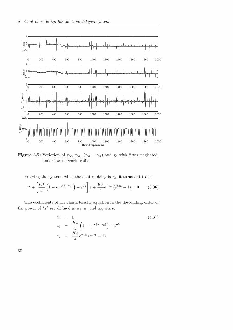
5 Controller design for the time delayed system
0 200 400 600 800 1000 1200 1400 1600 1800 20003
4
5
6
τ sc (
ms)
0 200 400 600 800 1000 1200 1400 1600 1800 20003
4
5
6
τ ca (
ms)
0 200 400 600 800 1000 1200 1400 1600 1800 2000−1
0
1
τ ca −
τ sc (
ms)
0 200 400 600 800 1000 1200 1400 1600 1800 20000
0.02
0.04
τ c (m
s)
Round trip number
Figure 5.7: Variation of τsc, τca, (τca − τca) and τc with jitter neglected,
under low network traffic
Freezing the system, when the control delay is τk, it turns out to be
z2 +
[
Kk
a
(
1− e−a(h−τk))
− eah]
z +Kk
ae−ah (eaτk − 1) = 0 (5.36)
The coefficients of the characteristic equation in the descending order of
the power of “z” are defined as a0, a1 and a2, where
a0 = 1 (5.37)
a1 =Kk
a
(
1− e−a(h−τk))
− eah
a2 =Kk
ae−ah (eaτk − 1) .
60

5.3 State Feedback Controller
0 200 400 600 800 1000 1200 1400 1600 1800 20007
8
9
10τ sc
(m
s)
0 200 400 600 800 1000 1200 1400 1600 1800 20007
8
9
10
τ ca (
ms)
0 200 400 600 800 1000 1200 1400 1600 1800 2000−2
0
2
τ ca −
τ sc (
ms)
0 200 400 600 800 1000 1200 1400 1600 1800 20000
0.02
0.04
τ c (m
s)
Round trip number
Figure 5.8: Variation of τsc, τca, (τca − τca) and τc with jitter neglected,
under high network traffic
For the system to be stable Jury’s stability conditions [28] applied are:
a0 > |an| (5.38)
P (z)|z=1 > 0 (5.39)
i.e., a0 + a1 + a2 > 0 (5.40)
P (z)|z=−1 > 0 (5.41)
i.e., a0 − a1 + a2 > 0 (5.42)
The necessary conditions required by the inequalities (5.39) and (5.42) and
the sufficient conditions obtained by forming the coefficient matrix [28], re-
61

5 Controller design for the time delayed system
sults in
τk <1
a
[
ln
∣
∣
∣
∣
1 +aeah
Kk
∣
∣
∣
∣
]
= τupper (5.43)
τk >1
a
[
ln
∣
∣
∣
∣
1
2
(
1−a
Kk
)(
1 + eah)
∣
∣
∣
∣
]
= τlower (5.44)
The inequality (5.39) gives eah > 1, which is identically true. Therefore to
maintain stability, boundary conditions have to be drawn for the sampling
interval h and the state feedback gain K. The τk is out of control but it has
to satisfy
max [τlower, 0] < τk < min [τupper, nh] , (5.45)
because 0 < τk < nh and n = 1, 2, 3.. depending on the amount of delay
that the system can tolerate while keeping the performance according to
specifications.
Conventionally, a faster sampling rate is desirable in sampled-data sys-
tems so that the discrete-time control design and its performance can ap-
proximate a near continuous time system i.e., sampling rates well above the
Nyquist sampling rate [24]. But in DCS, a faster sampling rate can increase
the network load, which in-tern results in longer delay of signals. Thus find-
ing a sampling rate that can both tolerate the network induced delay and
achieve the desired system performance is important in the design. How-
ever, for this specific application, the sampling rate has been fixed to 100 Hz
to achieve the desired transient performance of the motor. Hence the only
parameter that can be subjected to variation isK, which is obtained by pole-
placement design. The larger the distance of poles is from the origin, the
lesser the system is immune to noise. Therefore in addition to the stability
bounds for a given h, ultimate upper bound for K is defined by the system
noise level, which is not considered here, assuming the shielding provided is
sufficient to protect the system from noise hazards. Plotting the stability
region of the DCS with respect to h and τk is helpful to judge the possible
range of K. As it can be seen in Figure 5.9, for smaller sampling intervals the
system can tolerate larger delays up to nh. This should not be interpreted
as samples loose their chronological order in arriving the controller. But in
an event triggered system (except for sampling), it is the fact that when
62

5.3 State Feedback Controller
0 0.05 0.1 0.15 0.2 0.25 0.30
0.2
0.4
0.6
0.8
1
τ k/h
h (s)(a)
0 0.05 0.1 0.15 0.2 0.25 0.30
0.5
1
1.5
2
τ k/h
h (s)(b)
0 0.05 0.1 0.15 0.2 0.25 0.30
0.5
1
1.5
2
2.5
3
τ k/h
h (s)(c)
0 0.05 0.1 0.15 0.2 0.25 0.30
1
2
3
4
τ k/h
h (s)(d)
Figure 5.9: Stability region variation with the acceptable Control Delay
(a)τk = h, (b)τk = 2h, (c)τk = 3h and (d)τk = 4h with State
Feedback gain K = 5.0
∗ - Upper stability boundary, - Lower stability boundary
63
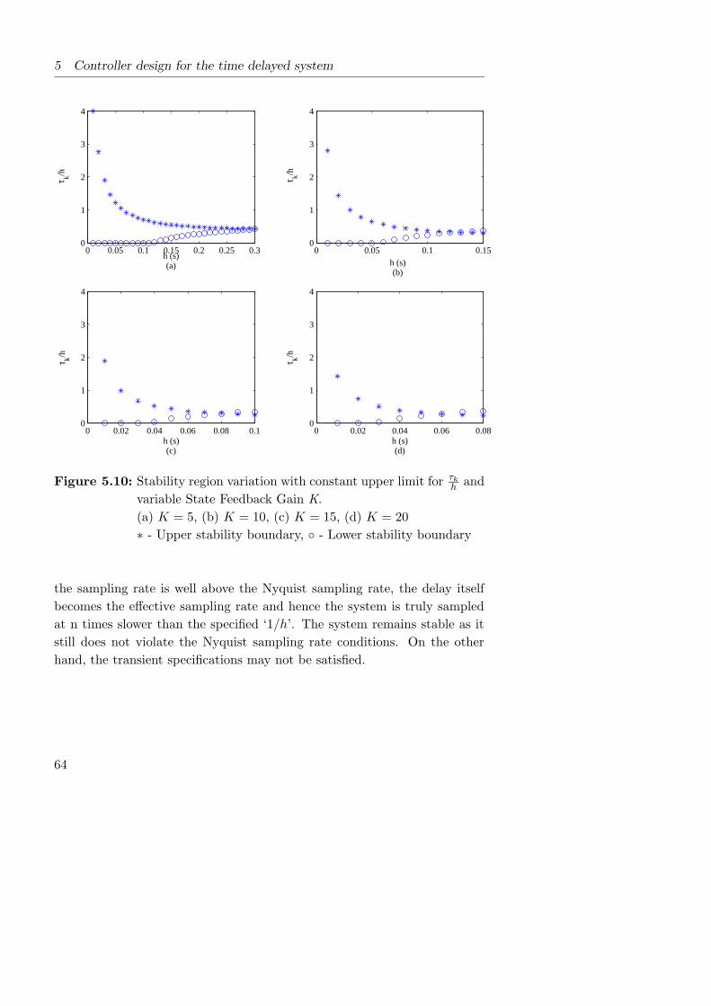
5 Controller design for the time delayed system
0 0.05 0.1 0.15 0.2 0.25 0.30
1
2
3
4
τ k/h
h (s)(a)
0 0.05 0.1 0.150
1
2
3
4
τ k/h
h (s)(b)
0 0.02 0.04 0.06 0.08 0.10
1
2
3
4
τ k/h
h (s)(c)
0 0.02 0.04 0.06 0.080
1
2
3
4τ k/h
h (s)(d)
Figure 5.10: Stability region variation with constant upper limit for τkhand
variable State Feedback Gain K.
(a) K = 5, (b) K = 10, (c) K = 15, (d) K = 20
∗ - Upper stability boundary, - Lower stability boundary
the sampling rate is well above the Nyquist sampling rate, the delay itself
becomes the effective sampling rate and hence the system is truly sampled
at n times slower than the specified ‘1/h’. The system remains stable as it
still does not violate the Nyquist sampling rate conditions. On the other
hand, the transient specifications may not be satisfied.
64

5.3 State Feedback Controller
The Figure 5.10 clearly shows that stability region is greatly reduced
with increased K. Hence the DCS can not be made faster beyond a limit
defined by the required sampling interval and the tolerable delay.
5.3.6 Estimator Design
Usually the purpose of an estimator is to determine the full states of the
plant to be controlled using partial state measurements. Additionally, in a
DCS, the partial measurements get delayed by τsck in reaching the estimator
node as shown in Figure 5.11. By the time the state measurements reach
the controller, the actual plant state may have changed. Therefore prior
to unknown states estimation, the estimator must evaluate the partial state
measurements pretending the states just before the control signal has been
released at the actuator node. This is essential as there is another delay τcakbefore the control signal reaches the actuator. The delay τcak is unknown
prior to the control signal computation and is therefore estimated from the
known τsck . The estimator is based on
x(t) = eA(t−t0)x(t0) +
∫ t
t0
eA(t−m)Bu(m) dm. (5.46)
The partial state measurement is the full state measurement as the system is
first order. According to Figure 5.11, from t = kh to t = kh+τk, the control
input is u((k−1)h). x(kh+τk) denotes the estimated plant state at the time
the control signal corresponding to state x(kh) reaches the actuator, then
x(kh+ τk) = eAτkx(kh) +
∫ kh+τk
kh
eA(kh+τk−m)Bu(m) dm. (5.47)
For the DCS concerned, the estimator turns out to be
x(kh+ τk) = eAτkx(kh) +k
a
[
1− e−aτk]
u(k − 1). (5.48)
65

5 Controller design for the time delayed system
(k−1)h kh (k+1)h
x(kh)
τca k
τc k
τsc k
x(kh+τ
Act
uato
r Es
timat
orC
ontro
ller
Proc
ess
Stat
e
u(kh+τ k )
)sck
τk
Figure 5.11: Timing data illustration at various nodes of the DCS
66
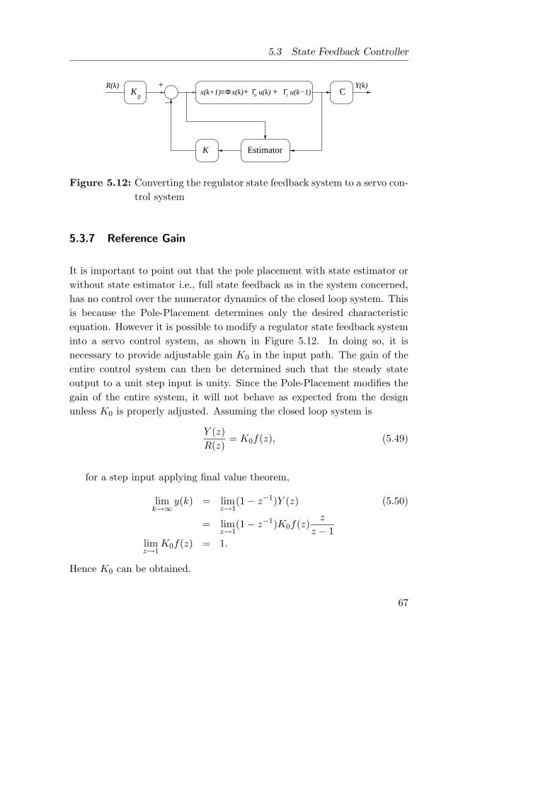
5.3 State Feedback Controller
x(k+1)=Φ x(k) Γ+ 0 u(k) Γ+ 1 u(k−1)+
−
K
K0
Estimator
CR(k) Y(k)
Figure 5.12: Converting the regulator state feedback system to a servo con-
trol system
5.3.7 Reference Gain
It is important to point out that the pole placement with state estimator or
without state estimator i.e., full state feedback as in the system concerned,
has no control over the numerator dynamics of the closed loop system. This
is because the Pole-Placement determines only the desired characteristic
equation. However it is possible to modify a regulator state feedback system
into a servo control system, as shown in Figure 5.12. In doing so, it is
necessary to provide adjustable gain K0 in the input path. The gain of the
entire control system can then be determined such that the steady state
output to a unit step input is unity. Since the Pole-Placement modifies the
gain of the entire system, it will not behave as expected from the design
unless K0 is properly adjusted. Assuming the closed loop system is
Y (z)
R(z)= K0f(z), (5.49)
for a step input applying final value theorem,
limk→∞
y(k) = limz→1
(1− z−1)Y (z) (5.50)
= limz→1
(1− z−1)K0f(z)z
z − 1limz→1
K0f(z) = 1.
Hence K0 can be obtained.
67

5 Controller design for the time delayed system
5.4 Results
Figure 5.13 compares the actual performances of different controller strate-
gies described in this chapter, for a time varying DCS. The PI controller
uses the parameters tuned off-line, despite the time variations caused by τ .
It also considers τ as a constant equal to its mean τmean.
The Smith predictor uses the Coefficient Diagram Method (CDM) in its
controller parameter calculations. The CDM produces a more stable con-
troller at presence of model errors due to its structure with higher degrees of
freedom. In this case too, τ is taken as constant. Both controllers are equally
good in minimizing the average steady state error, with tiny bursts even in
the steady state despite the integral action as the τk changes considerably
from its average. This is because both controllers have been tuned to the
average delay and in reality there are variations. Further the PI controller is
faster but has oscillations in the transients. The reason is that the numerical
integration in the PI controller increases in fixed steps expecting that the
control signal is applied to the actuator periodically. The period is supposed
to be the integrator time step. But it is not the case and is irregular in prac-
tice due to the time variations. The Smith predictor is smooth but slower
in transients. Because the error between the actual system and its model is
so large that the control signal is small and takes time to track the changes.
On the other hand, the State feedback controller has a comparatively
better steady state performance despite the lack of integral action. Further,
its transients are smoother and as fast as the PI controller. This is because
the time variations are treated on-line by the estimator.
It can be concluded that State feedback with on-line time delay com-
pensation produces a comparatively better controller for the time varying
distributed control system containing the first order plant. Further, the
Brushless DC motor with this controller can be used for a precise speed
control application in a distributed system.
68

5.4 Results
500 550 600 6500.2
0.4
0.6
0.8
1
Sample (a)
Spee
d (V
)
2450 2500 2550 2600 26500.2
0.4
0.6
0.8
1
Sample(b)
Spee
d (V
)
500 550 600 6500.2
0.4
0.6
0.8
1
Sample(c)
Spee
d (V
)
2450 2500 2550 2600 26500.2
0.4
0.6
0.8
1
Sample(d)
Spee
d (V
)
Figure 5.13: Performance comparison of different controller strategies,
State feedback controller (—) vs PI controller (- -);
(a) Speed increment, (b) Speed decrement.
State feedback controller (—) vs Smith predictor (-.-);
(c) Speed increment, (d) Speed decrement.
69

5 Controller design for the time delayed system
70
6 Speed Synchronization
Maintaining speed synchronism among several motor drives undergoing
torque disturbances is considered as a suitable application to adapt the dis-
tributed speed controller with on-line delay compensation derived in Chap-
ter 5. It is studied theoretically in this chapter.
6.1 Introduction
In the motion control industry, the term synchronization is used often so
interchangeably with the term master-slave. In a master-slave system, one
machine works as the virtual master and one or many machines follow the
master as virtual slaves. Any change in the speed/position of the master is
immediately induced among the slaves, all in the same manner or in different
degrees depending on the application. The most common question in the
master-slave configuration is, “What happens if a slave undergoes a change
in speed/position due to a torque disturbance?”. In most industrial appli-
cations this is an unanswered question that eventually results in defective
products.
The synchronization described in this report has neither a master nor
slaves. But all the machines have equal privileges. Whenever any one of
them encounter a disturbance on its shaft, it is reflected to the rest of the
machines working in parallel either with a minimum synchronizing error or
71

6 Speed Synchronization
with a minimum tracking error. Hence it is aimed to answer the above
question constructively.
6.2 Application Aspects
The speed/position synchronization has many promising industrial applica-
tions, where motion control can be utilized to reduce, both the capital and
maintenance costs, most of all the plant down time and the percentage of
defectives. Some of these applications are summarized below.
6.2.1 Offset Printing
Offset printing traditionally uses a mechanical line shaft to synchronize the
different color printing stations. The mechanical devices involved require
high maintenance, and the system is limited in speed.
The mechanical line shaft system can be replaced with individual ser-
vomotors (Figure 6.1) that can be synchronized precisely through the dis-
tributed motion control technology. Communication to higher level controls,
evaluation of system status and drive set-point signals, can be accomplished
with Ethernet/IP (Industrial Protocol), i.e., the same Ethernet protocol but
with more robust hardware suitable for rough use in industry [39].
6.2.2 Horizontal Bagging
This application involves a continuous roll of foil for horizontal bagging (Fig-
ure 6.2). The sealing station handles the foil transport. Electronic line shaft
and print mark registration ensure the foil is synchronized with the products
being packaged. Electronic line shafting also ensures the product feeder belt
and the foil are in continuous position synchronization. Print mark registra-
tion will accelerate or decelerate the foil to make up for the possible stretch.
72

6.2 Application Aspects
Figure 6.1: Offset printing press using motors in place of mechanical links
for synchronization [40]
This ensures that printed labels on the foil will be correctly positioned on
the package despite any disturbance torque in any of the motors involved.
6.2.3 Cut to Length Rotary Knife
The purpose is to cut material to a precise length. For a fixed cut length, and
a knife circumference of the same length, it is simply a matter of maintaining
a constant speed between the web and the knife. However, for products that
require various cut lengths, the knifes circumference would have to vary to
match these cut lengths. Since this would not be practical, the knife speed
is often profiled. By varying the knife speed, various cut lengths can be
obtained. Furthermore, the rotary knife is accelerated so that, the cutting
73
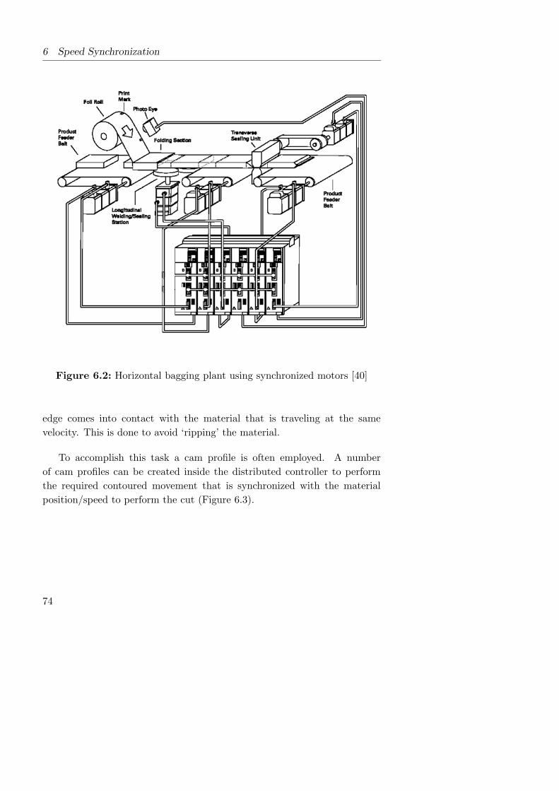
6 Speed Synchronization
Figure 6.2: Horizontal bagging plant using synchronized motors [40]
edge comes into contact with the material that is traveling at the same
velocity. This is done to avoid ‘ripping’ the material.
To accomplish this task a cam profile is often employed. A number
of cam profiles can be created inside the distributed controller to perform
the required contoured movement that is synchronized with the material
position/speed to perform the cut (Figure 6.3).
74

6.2 Application Aspects
Figure 6.3: Synchronized motors in precise material cutting [40]
6.2.4 Pick and Place
Pick and Place applications involve the precise movement of product from
one location to another. Typically the gripper claw is ‘homed’ to the starting
location during the initialization of the system. From that point, as product
is sensed, the gripper closes on it and the move is made. Once the final
destination point is reached the gripper releases the product and returns to
the home position. It allows easy sending of all the appropriate status and
control signals from one axis drive to the next.
The point-to-point positioning feature of any commercial motor drive will
be capable of meeting this performance demand. Adding the two-way syn-
chronization will further improve the flexibility of the drive while minimizing
the speed/position errors and hence the defectives.
75

6 Speed Synchronization
Figure 6.4: Precise object placement using synchronized motors [40]
6.3 Approach
In the literature, many work related to position synchronization can be found
using control techniques such as scalar field theorem [42] and adaptive control
theory [43], where the steady state performance is very well guaranteed but
not the transient performance. Since the goal of this work is to reflect the
impact of a torque disturbance on the speed of one machine to another
machine running parallel, emphasis will be both on the steady state as well
as the transient speed response, both in non-distributed and distributed
speed synchronization.
6.3.1 Master Slave
This is the well known synchronizing method that has been in practice for
decades. The basic block diagram configuration is shown in Figure 6.5 . The
impact of Td1 on ω1 will be reflected at ω2, provided that two controllers have
been tuned accordingly, but not vice versa. Further ω2 always lags ω1, which
76

6.3 Approach
Td1
ωController 1 Motor 1
−Controller 2 Motor 2
ω2ref +
−
−
+
ω1+
Figure 6.5: Speed synchronization : Master-slave configuration
could be seen during starting-stopping and disturbance transients. Due to
inherent temporal constraints, in the distributed version, the ω2 will further
be delayed in addition to cross coupling disability.
6.3.2 Interactive Feedback Control
This method is an extension to the work found in [41] on cross coupling
position control. The term tracking error is defined as the difference between
the reference speed and the actual speed of each speed control loop, while
synchronizing error is the difference between the actual speeds of the two
speed control loops. The concept in Interactive Feedback Control is to use
the synchronizing error to couple the speed variation on one machine to
another via the reference speed. When there is no disturbance torque, the
speeds are equal and each machine has an effective state feedback gain of
K (Figure 6.6). But when one machine is disturbed, the synchronizing
error acts as a positive feedback on that machine while imposing a negative
feedback on the undisturbed one. Hence the disturbed one is accelerated,
while the other is decelerated. Thus the synchronizing error is expected to
be kept minimum.
The plant under consideration of this report is an open loop first order
system and the most suitable controller derived for distributed operation
in Chapter 5 is full-state feedback with a delay compensation. The overall
system still remains as first order. Even though it is suitable to achieve the
desired transient performance in the absence of disturbances on the shaft,
measures have to be taken to avoid such steady state speed errors in the
77

6 Speed Synchronization
K0
KPz IK+z −1
Γ C
Φ
K H+
H
H
K H+
KPz IK+z −1
Γ
Φ
CK0
Td1
Y1 (k)
Td2
Y2 (k)
R (k)
R (k)
+
+
+
−
−
+
+
+
+
+z−1I
−
z−1I−
Figure 6.6: Speed synchronization for non-distributed motors
presence of torque disturbances. Therefore an integrator is introduced by
means of a PI controller. The block diagram of the non-distributed version
is shown in Figure 6.6.
When the system is in steady state under the common reference speed
R(k), applying a step disturbance of amplitude Td1 on the first machine
78

6.3 Approach
results in the following system equations,
−zTd1 = [(z − Φ)(z − 1) + (KP z +KI)(H +K)]x1(k)
− (KP z +KI)Hx2(k) (6.1)
0 = [(z − Φ)(z − 1) + (KP z +KI)(H +K)]x2(k)
− (KP z +KI)Hx1(k). (6.2)
The system equations can be reduced to
[
x1 (k)
x2 (k)
]
=γ
α2 − β2
[
α
−β
]
, (6.3)
where
α = (z − Φ)(z − 1) + (KP z +KI)(H +K) (6.4)
β = −(KP z +KI)H
γ = −zTd1.
Hence the only way to keep x2 (k) as close as possible to x1 (k) is by making
K as small as possible and H as high as possible within the stability bounds
derived in Chapter 5. Further this selection criteria is a compromise between
the tolerable synchronizing error and the speed of the response. In the
simulation, a torque disturbance is first applied on Motor1 at time=5 s
and the second disturbance is applied on Motor2 at time=10 s before the
transient of the first disturbance is completely over. It can be seen clearly in
Figure 6.7 that in steady state, both the synchronizing error and the tracking
error become zero but at the price of slow response.
6.3.3 Synchronization in distributed systems
For the distributed speed control, the system has to be provided with a state
estimator using previous control signals, delayed speed measurements and
the time delay (as derived in Chapter 5). The discrete time system block
diagram is shown in Figure 6.8. In the presence of the disturbance Td, the
79

6 Speed Synchronization
0 5 10 15 20
0.2
0.4
0.6
0.8
1
time (s)
Spee
d re
spon
se (
V)
Motor1Motor2
0 5 10 15 20
−0.06
−0.04
−0.02
0
0.02
0.04
0.06
Syn
chro
nizi
ng s
peed
err
or (
V)
time (s)
Figure 6.7: Synchronized speed responses for non-distributed motors
system can be derived as
[zΓ0 + Γ1][KP z +KI ][R(z)−M1X(z)]
[(z − 1) +M0(KP +KIz)]− (z − Φ)X(z) = Td. (6.5)
Hence the steady state tracking error becomes
Ess =KM0
(I − Φ)KM0 + (Γ0 + Γ1)M1, (6.6)
80

6.3 Approach
Td1
Y1 (k)z−1I
1z
KPz IK+z −1
M0
M1
Γ1
Γ0K
0
R (k) +
+
C
Φ
+
+
+
−
K
+
++
Figure 6.8: Distributed controlled motor with delay compensation
where
Φ = e−ah (6.7)
Γ0 =k
a[1− e−a(h−τ)]
Γ1 =k
a[e−a(h−τ) − e−ah]
M0 =k
a[1− e−aτ ]
M1 = e−aτ .
Substituting the above values into equation (6.6) results in the steady
state tracking error as
Ess =(1− e−aτ )Td
(1− e−ah)(1− e−aτ ) + ae−aτ
Kk(1− e−ah)
, (6.8)
which is dependent upon the system dynamics, disturbance amplitude and
the delay, but it vanishes when the delay is zero. Examining the block
diagram in Figure 6.8 reveals that the cause of the non-zero tracking error
is the path for the estimator from the previous control inputs, via M0. To
81
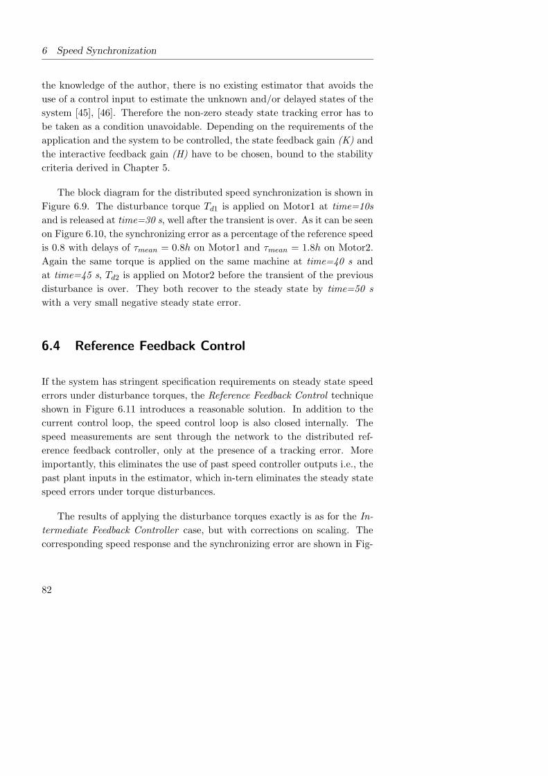
6 Speed Synchronization
the knowledge of the author, there is no existing estimator that avoids the
use of a control input to estimate the unknown and/or delayed states of the
system [45], [46]. Therefore the non-zero steady state tracking error has to
be taken as a condition unavoidable. Depending on the requirements of the
application and the system to be controlled, the state feedback gain (K) and
the interactive feedback gain (H) have to be chosen, bound to the stability
criteria derived in Chapter 5.
The block diagram for the distributed speed synchronization is shown in
Figure 6.9. The disturbance torque Td1 is applied on Motor1 at time=10s
and is released at time=30 s, well after the transient is over. As it can be seen
on Figure 6.10, the synchronizing error as a percentage of the reference speed
is 0.8 with delays of τmean = 0.8h on Motor1 and τmean = 1.8h on Motor2.
Again the same torque is applied on the same machine at time=40 s and
at time=45 s, Td2 is applied on Motor2 before the transient of the previous
disturbance is over. They both recover to the steady state by time=50 s
with a very small negative steady state error.
6.4 Reference Feedback Control
If the system has stringent specification requirements on steady state speed
errors under disturbance torques, the Reference Feedback Control technique
shown in Figure 6.11 introduces a reasonable solution. In addition to the
current control loop, the speed control loop is also closed internally. The
speed measurements are sent through the network to the distributed ref-
erence feedback controller, only at the presence of a tracking error. More
importantly, this eliminates the use of past speed controller outputs i.e., the
past plant inputs in the estimator, which in-tern eliminates the steady state
speed errors under torque disturbances.
The results of applying the disturbance torques exactly is as for the In-
termediate Feedback Controller case, but with corrections on scaling. The
corresponding speed response and the synchronizing error are shown in Fig-
82
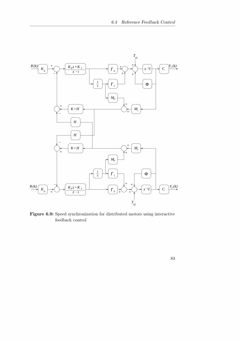
6.4 Reference Feedback Control
Td1
Y1 (k)z−1I
1z
KPz IK+z −1
M0
M1K H+
H
H
K H+ M1
M0
Γ1
Γ0
Γ1
1z
KPz IK+z −1
Γ0
Td2
z−1I
Φ
CY2 (k)
K0
R (k)
K0
R (k)
+
+
C
Φ
+
+
+
−
+
+
+
+
+
+
+
−
−
+
+
−
+
+
Figure 6.9: Speed synchronization for distributed motors using interactive
feedback control
83

6 Speed Synchronization
0 10 20 30 40 50 60
0.5
1
1.5
time (s)
Spee
d re
spon
se (
V)
Motor1Motor2
0 10 20 30 40 50 60
−0.05
0
0.05
Syn
chro
nizi
ng s
peed
err
or (
V)
time (s)
Figure 6.10: Speed responses of the distributed speed synchronization us-
ing interactive feedback control
Td1
Y1 (k)
Td2
Y2 (k)
K0
R (k)
M1K H+
z−1I
z−1I C
Φ
Γ
KPz IK+z −1
KPz IK+z −1
K H+ M1
H
H
K0
R (k)
1z
M0
1z
M0
+
+
+
+
+
−
+
−
+Γ C
−
Φ+
+
−
+
−
+
++
τca1
τsc1
τsc2
τca2
Figure 6.11: Distributed speed synchronization using reference feedback
control
84
6.4 Reference Feedback Control
0 10 20 30 40 50 60
0.2
0.4
0.6
0.8
1
1.2
1.4
1.6
time (s)
Spee
d re
spon
se (
V)
Motor1Motor2
0 10 20 30 40 50 60−0.3
−0.2
−0.1
0
0.1
0.2
Syn
chro
nizi
ng s
peed
err
or (
V)
time (s)
Figure 6.12: Speed responses of the distributed speed synchronization us-
ing reference feedback control
ure 6.12. It can clearly be seen that the steady state speed error is always
zero and the responses are much faster. Even though this method is contra-
dictory to the entire DCS concept, this will be appropriate for bandwidth
restricted DCSs.
85

6 Speed Synchronization
86

7 Conclusions and future work
The conclusions of the study and the future work are presented in this chap-
ter.
7.1 Conclusions
The time delay problem of the motion control system distributed via the
standard 10 Mbps Switched Ethernet network is studied using the following
controller strategies both theoretically and experimentally.
1. Standard Proportional Integral (PI) controller with suitable tuning
techniques for time delayed systems.
2. Smith Predictor controller modified by Coefficient Diagram Method
(CDM) to cater delay model inaccuracies and to achieve higher degrees
of freedom in the controller.
3. State feedback controller using on-line delay compensation.
The first two strategies use the mean delay of the network, calculated off-line,
while the third uses the actual control delay computed as the sum of
1. Sensor to controller delay (τsc)
87

7 Conclusions and future work
2. The predicted controller to actuator delay based on the characteristics
of the network (τca)
3. The controller execution time (τc) and jitter
neglecting the variation of jitter.
The PI controller is originally for non-time delayed systems, but modified
to work as a robust controller with time delays. Further it is recommended
only for τ < h. The Smith Predictor is inherently for time delayed systems
with τ >> h. Hence these two controllers are used to establish the lower
and upper boundary solutions for the variable time delayed system. Due to
the change of instantaneous state of the network, the delay
• Is not constant
• Does not necessarily satisfy τ < h
• Does not necessarily satisfy τ >> h.
Therefore it is necessary to design the controller regardless of the magnitude
of the delay. The state feedback controller, whose delayed states are esti-
mated using the system dynamics in a linear estimator, gives a satisfactory
transient closed loop performance.
It has to be emphasized that the maximum tolerable delay is system
dependent and is relative to the desired closed loop dynamics and hence the
sampling interval. Therefore in general a suitable stability analysis must be
carried out in defining the bounds of sampling interval, state feedback gain
and the tolerable delay. In this study, Jury’s stability criteria is used.
The results of the delay compensated state feedback distributed con-
troller are applied in speed synchronizing two Brushless DC motors.
The speed synchronization is first studied using the non-distributed ver-
sion of the system. The state feedback controller is then extended for
88
7.2 Future work
the speed synchronization introducing interactive feedback controller whose
gains are tuned to achieve minimum possible synchronizing errors. This
method together with the state feedback controller with delay compensation
is applied for the distributed version of the speed synchronization. The tran-
sient performance is satisfactory as expected but the steady state speed of
the motor, which underwent the torque disturbance, is with a minor steady
state error.
The above mentioned error is caused by the delay compensating state
estimator, and is dependent exponentially upon the delay and the system
time constant. To cater systems with stringent requirement specifications,
which do not accept even such minor steady state errors that last only during
the period under disturbances, the Reference Feedback control is introduced.
This results in zero steady state error but with a higher synchronizing error
only at the peak dropout in speed of the motor which underwent the dis-
turbance. Therefore whether to choose the Interactive feedback control or
Reference feedback control must be based on the specifications of the partic-
ular drive system.
7.2 Future work
The distributed version of the speed synchronization experiments is lim-
ited to simulations due to implementation problems in the controller. The
TCP/IP software has a single copy residing in the operating system, which
is Red Hat Linux 7.2 in this case. When it is invoked by independent mul-
tiple programs, in a single processor system, the CPU context is switched
so rapidly, giving the illusion that multiple programs are executed simul-
taneously. This mechanism is strictly restricted for multiple independent
programs without data dependency i.e., no data transfer is allowed between
independent programs [13].
The physical implementation of the distributed version of the speed syn-
chronization comprises three main programs. The first two are for the dis-
89

7 Conclusions and future work
tributed closed loop operation of each motor, while the third is to couple the
speed of one motor to the other and vice versa through the synchronizing
controller. Hence the three programs are data dependent and can not be
implemented in a single processor system sharing the TCP/IP, unless the
operating system can be modified to do so.
An alternative approach is to implement all three loops in a single pro-
gram. Then a single program has to establish and maintain two TCP sockets,
which seem to be independent, but having an interactive communication by
means of dependent data transfers, which is again not allowed within the
scope of TCP/IP in normal operating systems. Further, this method limits
the scalability of the DCS.
Hence it is required to divert the attention to a new Real-Time Operating
System (RTOS) environment with the following main features.
• Fully functional support for TCP/IP with inter-thread communication,
despite data dependency.
• Real-Time task execution capability with dynamic scheduling, pre-
emptive multi-tasking and priority inversion capabilities.
• x686 processor compatibility.
90
References
[1] J. Nilsson, “Real-Time Control systems with delays”, Doctoral thesis,
Lund Institute of Technology, Lund Sweden 1998.
[2] W. Zhang, M. S. Branicky, S. M. Philips, “Stability of Networked Control
Systems”, in IEEE Control Systems Magazine February 2003, pp 84-93.
[3] J. Nilsson, B. Bernhardsson, B. Wittenmark, “Stochastic Analysis and
Control of Real-Time Systems with Random Time Delays”, in Proceeding
of 13th International Federation of Automatic Control world congress
1996, San Francisco, pp 267-272.
[4] R. Perlman, “Interconnections, Bridges, Routers, Switches and Inter-
networking Protocols”, Second Edition, Addison Wesley 2000.
[5] E. Altman, T. Basar, R. Srikant, “Congestion Control as a Stochastic
Control Problem with Action Delays”, in Automatica December 1999,
vol.35,pp1937-1950.
[6] S. Mascolo, “Classical Control Theory for congestion avoidance in High
Speed Internet”, in Proceedings of IEEE Decision Control Conference
1999, Phoenix, pp.2709-2714.
[7] K. S. Walgama, D. G. Fisher, S. L. Shah, “Control of Processes with
Noise and Time Delays”, in Proceedings of International Chemical En-
gineering Journal, February 1989, vol.35,No.2,pp 213-222
[8] J. Nilsson, B. Bernhardsson, B. Wittenmark, “Some topics in Real-Time
Control”, in Proceedings of American Control Conference Pennsylvania
1998.
91

References
[9] A. Ray, “Introduction to Networking for Integrated Control Systems”,
in IEEE Control Systems Magazine 1989, pp.76-79.
[10] J. D. Decotignie, “A Perspective On Ethernet TCP/IP as a Fieldbus”,
in Proceedings of 4th IFAC Conference on Fieldbus systems, France, 2001,
pp.138-142.
[11] C. K. Lee, W. H. Pang, “Brushless DC Motor Speed Control System
Using Fuzzy Rules”, in Proceedings of Power Electronics and Variable-
Speed Drives Conference 1994, pp.101-106.
[12] B. K. Bose, “Modern Power Electronics and AC Drives Vol II”, Third
Edition, Prentice Hall Inc, 2000.
[13] D. E. Comer, D. L. Stevens, “Internetworking with TCP/IP”, Third
Edition, Prentice Hall Inc, 2000.
[14] W. Stalling, “Data and Computer Communication”, Sixth Edition,
Prentice Hall Inc, 2000.
[15] W. R. Stevens, “TCP/IP Illustrated Vol I”, Addison Wesley, 1994.
[16] S. Varadarajan, T. Chiueh, “EtheReal : A Host - Transparent Real-
Time Fast Ethernet Switch”, Department of Computer Science, State
University of New York, 2001.
[17] U. Hagstrom, A. Kallerdahl, “Switched Industrial Real-Time Ethernet”,
Master Thesis, Halmstad University, Halmstad, Sweden 2001.
[18] “IPv6 Standard”, Internet Engineering Task Force, Toronto, 1994.
[19] N. D. Aakvaag, N. A. Nordbotton, “IPv6 The New Internet Protocol”,
ABB Review, The corporate technical journal of ABB Group, Sweden
2003.
[20] M. Torngren, “Modeling and design of distributed real-time control ap-
plications”, Doctoral thesis, Royal Institute of Technology, Stockholm,
Sweden 1995.
92
[21] “Dynamic C Premier 7.02”, Programming Guide, Z-World Inc, Cali-
fornia, USA.
[22] “C-Programmable Single-Board Computer with Ethernet and Operator
Interface”, User Manual, Z-World Inc, California, USA.
[23] “Advanced Motion Control - PWM Servo Amplifiers”, Technical Man-
ual, Ostergrens Elmotor AB, Bromma, Sweden.
[24] K. J. Astrom, B. Wittenmark, “Computer-Controlled Systems”, Third
edition. Prentice Hall,1997.
[25] K. Shin, X. Cui, “Computing Time Delay and its Effects on Real-Time
Control Systems”, in IEEE Transactions on Control Systems Technology
1996, Vol. 3, N. 2, pp 218-224.
[26] B. Wittenmark, J. Nilsson, M. Torngren, “Timing Problems in Real-
Time Control Systems”, in Proceedings of American Control Conference,
1995.
[27] B. Bastian, “Analysis of Time Delays in Synchronous and Asyn-
chronous Control Loops”, Master thesis, Department of Automatic Con-
trol, Lunds Institute of Technology, Sweden.
[28] K. Ogata, “Discrete Time Control Systems”, Third Edition, Prentice
Hall 2000.
[29] A. O’Dwyer, “The estimation and compensation of processes with time
delays”, Doctoral thesis, Dublin City University, 1996.
[30] S. Bentouati, Z. Q. Zhu, D. Howe, “Permanent Magnet Brushless
DC Motors for Consumer Products,” Technical Report, University of
Sheffield, U.K
[31] J. G. Ziegler, N. B. Nichols, “Optimum settings for automatic con-
trollers”, in Transactions of the ASME 1942, Vol. 64, pp 759-768.
[32] G. F. Franklin, J. D. Powell, M. Workman, “Digital Control of Dynamic
Systems”, Third Edition, Addison Wesley 1997.
93
References
[33] A. O’Dwyer, “Performance and robustness issues in the compensation
of FOLPD processes with PI and PID controllers”, in Proceedings of
Irish Signals and Systems Conference, Dublin Institute of Technology,
Dublin, Ireland, June 1998.
[34] J. Syder, T. Heeg, A. O’Dwyer, “Dead-time compensators: performance
and robustness issues”, School of Control Systems and Electrical Engi-
neering, Dublin Institute of Technology, Dublin, Ireland.
[35] K. S. Walgama, “On the Control Systems with Input Saturation or
Periodic Disturbances”, Doctoral thesis, Lulea University of Technology,
Lulea Sweden 1992.
[36] S. Alahakoon, “Digital Motion Control Techniques for Electrical
Drives”, Doctoral thesis, Royal Institute of Technology, Stockholm, Swe-
den 2000.
[37] S. E. Hamamchi, I. Kaya, D. P. Atherton, “Smith Predictor Design by
CDM”, in Proceedings of the European Control Conference 2001.
[38] S. Manabe, “Application of Coefficient Diagram Method to MIMO de-
sign in aerospace”, in Proceedings of the 15th Triennial IFAC World
Congress, Barcelona, Spain 2002.
[39] M. Daniels, “Ethernet/IP Industrial Standard - Open, Available and
Based on Modern Technology” in the Proceedings of Drives and Controls
Exhibition and Conference, London 2001, ISBN 1-901672-53-0
[40] “Industrial Communication for Automation” SIEMENSTM Automa-
tions and Drives Group Magazine, April 2001.
[41] L. Feng, Y. Koren, J. Borenstien, “Cross-Coupling Motion Controller
for Mobile Robots”, in IEEE Control System Magazine December 1993.
[42] R. Danbury, M. Jenkinson, “Synchronized Servomechanisms - the scalar
field approach”, in IEE Control Theory Applications magazine, vol 141,
No 4, July 1994.
94

[43] D. Sun, “Position Synchronization of Multiple Motion Axes with Adap-
tive Coupling Control”, in Proceedings of the 15th IFAC World Congress,
Barcelona, Spain 2002.
[44] J. Yook, D. Tilbury, K. Chervela, N. Soparkar, “Decentralized, Mod-
ular Real-Time Control for Machining Applications”, Project Report,
Mechanical Engineering and Applied Mechanics, University of Michigan,
USA, 1997.
[45] O. Sename, “Unknown Input Robust Observers for Time-Delay Sys-
tems”, in Proceedings of IEEE Decision and Control Conference, Cali-
fornia, USA, 1997.
[46] A. Fattouh, O. Sename, J. Dion, “An Unknown Input Observer Design
for Linear Time-Delay Systems”, in Proceedings of IEEE Decision and
Control Conference, Arizona, USA, 1999.
95

References
96
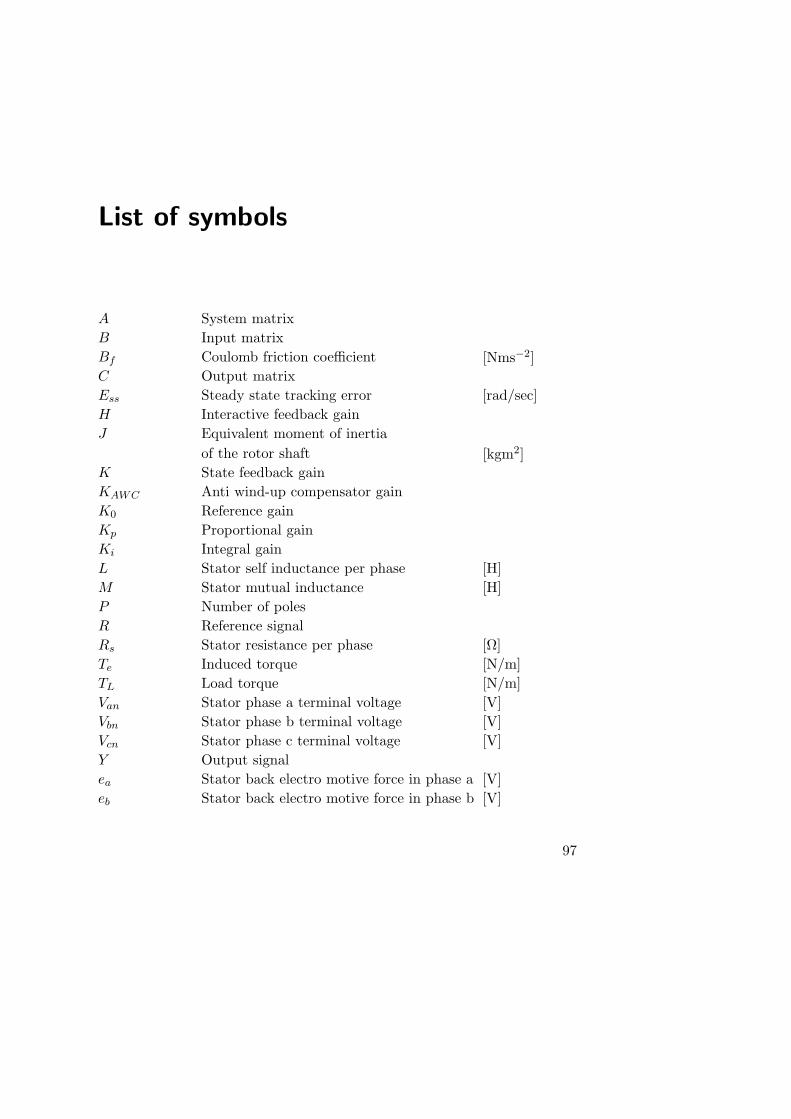
List of symbols
A System matrix
B Input matrix
Bf Coulomb friction coefficient [Nms−2]
C Output matrix
Ess Steady state tracking error [rad/sec]
H Interactive feedback gain
J Equivalent moment of inertia
of the rotor shaft [kgm2]
K State feedback gain
KAWC Anti wind-up compensator gain
K0 Reference gain
Kp Proportional gain
Ki Integral gain
L Stator self inductance per phase [H]
M Stator mutual inductance [H]
P Number of poles
R Reference signal
Rs Stator resistance per phase [Ω]
Te Induced torque [N/m]
TL Load torque [N/m]
Van Stator phase a terminal voltage [V]
Vbn Stator phase b terminal voltage [V]
Vcn Stator phase c terminal voltage [V]
Y Output signal
ea Stator back electro motive force in phase a [V]
eb Stator back electro motive force in phase b [V]
97
List of symbols
ec Stator back electro motive force in phase c [V]
h Sampling interval [s]
I Identity matrix
ia Stator phase a current [A]
ib Stator phase b current [A]
ic Stator phase c current [A]
u Controller output
v Reset output
ωe Rotor electrical speed [rad/sec]
ωr Rotor mechanical speed [rad/sec]
γi Stability indices
τ Absolute control delay [s]
τlower Lower bound of the control delay [s]
τmean Mean control delay [s]
τupper Upper bound of the control delay [s]
τsc Sensor to controller delay [s]
τca Controller to actuator delay [s]
98