Distributed Beamforming in Wireless Relay Networks
86
Distributed Beamforming in Wireless Relay Networks by Siavash Fazeli-Dehkordy A thesis submitted to the Department of Electrical and Computer Engineering in conformity with the requirements for the degree of Master of Science (Engineering) Queen’s University Kingston, Ontario, Canada September 2008 Copyright c Siavash Fazeli-Dehkordy, 2008
Transcript of Distributed Beamforming in Wireless Relay Networks
Distributed Beamforming in Wireless Relay
Networks
by
Siavash Fazeli-Dehkordy
A thesis submitted to the
Department of Electrical and Computer Engineering
in conformity with the requirements for
the degree of Master of Science (Engineering)
Queen’s University
Kingston, Ontario, Canada
September 2008
Copyright c© Siavash Fazeli-Dehkordy, 2008
Abstract
In this thesis, we consider a wireless network consisting of d source-destination pairs
and R relaying nodes. Each source wishes to communicate to its corresponding desti-
nation. By exploiting the spatial multiplexing capability of the wireless medium, we
develop two cooperative beamforming schemes in order to establish wireless connec-
tions between multiple source-destination pairs through a collaborative relay network.
Our first communication scheme consists of two steps. In the first step, all sources
transmit their signals simultaneously to the relay network. As a result, each relay re-
ceives a noisy faded mixture of all source signals. In the second step, each relay trans-
mits an amplitude- and phase-adjusted version of its received signal, i.e., the relay
received signals are multiplied by a set of complex coefficients and are retransmitted.
Our goal is to obtain these complex coefficients (beamforming weights) through min-
imization of the total relay transmit power while the signal-to-interference-plus-noise
ratio at the destinations are guaranteed to be above certain pre-defined thresholds.
Our second scheme is a distributed downlink beamforming technique which is
performed in d + 1 successive time slots. In the first d time slots, the d sources
transmit their data to the relay network successively. The relay nodes receive and
store the noisy faded versions of the source signals. In the (d + 1)th time slot, the
relays aim to collectively provide downlink connections to all d destinations. To do
i

so, each relay transmits a linear combination of the stored signals received during the
first d time slots. Again, our goal is to determine the complex weights (used at the
relaying nodes to linearly combine the source signals) by minimizing the total relay
transmit power while satisfying certain quality of services at the destinations.
We use semi-definite relaxation to turn both problems into semi-definite program-
ming (SDP) problems. Therefore, they can be efficiently solved using interior point
methods. We showed that our proposed schemes significantly outperform orthogonal
multiplexing schemes, such as time-division multiple access schemes, in a large range
of network data rates.
ii
Acknowledgments
It has been an exceptional experience to benefit from the supervision of Professor
Saeed Gazor, and Professor Shahram Shahbazpanahi. I am very grateful to Professor
Gazor for his insight, encouragement, and dedication to the personal and professional
growth of his graduate students. My deepest gratitude goes to Professor Shahbaz-
panahi for his endless help, guidance, and inspiration during the course of my work.
Despite the distance between Queen’s University and UOIT, he has been a patient
teacher and an excellent adviser. It is hard to imagine having done my M.Sc. with-
out his unconditional support. I am also indebted to the other members of my thesis
committee, Professor Il-Min Kim, Professor Glen Takahara, Professor Tom Dean, and
Professor Richard Henriksen, for their valuable time and interest in my work.
Special thanks to my colleagues in the Advanced Multidimensional Signal Pro-
cessing Laboratory for our inspiring discussions, friendship, and enjoyable moments
over the past two years.
Finally, I would like to extend my deepest gratitude to my parents, my sisters,
and my grandparents for their never-ending love, support, and encouragement.
iii

Table of Contents
Abstract i
Acknowledgments iii
Table of Contents iv
List of Figures vi
Chapter 1:
Introduction . . . . . . . . . . . . . . . . . . . . . . . . . . 1
1.1 Cooperative Communications . . . . . . . . . . . . . . . . . . . . . . 1
1.2 Thesis Contributions . . . . . . . . . . . . . . . . . . . . . . . . . . . 2
1.3 Thesis Outline . . . . . . . . . . . . . . . . . . . . . . . . . . . . . . . 4
1.4 Notations . . . . . . . . . . . . . . . . . . . . . . . . . . . . . . . . . 5
Chapter 2:
Background . . . . . . . . . . . . . . . . . . . . . . . . . . 6
2.1 Multi-Antenna Communication Systems . . . . . . . . . . . . . . . . 6
2.2 Multiuser Systems . . . . . . . . . . . . . . . . . . . . . . . . . . . . 8
2.3 Receive and Transmit Beamforming . . . . . . . . . . . . . . . . . . . 9
2.4 Cooperative Schemes in Wireless Networks . . . . . . . . . . . . . . . 15
iv

Chapter 3:
A Multiple Peer-to-Peer Communication Scheme in Wire-
less Relay Networks . . . . . . . . . . . . . . . . . . . . . 18
3.1 Introduction . . . . . . . . . . . . . . . . . . . . . . . . . . . . . . . . 18
3.2 Data Model . . . . . . . . . . . . . . . . . . . . . . . . . . . . . . . . 19
3.3 Power Minimization . . . . . . . . . . . . . . . . . . . . . . . . . . . . 22
3.4 Individual Relay Power Constraints . . . . . . . . . . . . . . . . . . . 27
3.5 Simulation Results . . . . . . . . . . . . . . . . . . . . . . . . . . . . 28
Chapter 4:
A Distributed Downlink Beamforming Scheme in Wire-
less Relay Networks . . . . . . . . . . . . . . . . . . . . . 44
4.1 Introduction . . . . . . . . . . . . . . . . . . . . . . . . . . . . . . . . 44
4.2 Problem Formulation . . . . . . . . . . . . . . . . . . . . . . . . . . . 45
4.3 Power Minimization . . . . . . . . . . . . . . . . . . . . . . . . . . . . 48
4.4 Simulation Results . . . . . . . . . . . . . . . . . . . . . . . . . . . . 52
Chapter 5:
Conclusions and Future Work . . . . . . . . . . . . . . . 58
Bibliography . . . . . . . . . . . . . . . . . . . . . . . . . . . . . . . . . 61
Appendix A:
Semidefinite Relaxation and The Duality Gap . . . . . 67
Appendix B:
Proof of Lemma 1 . . . . . . . . . . . . . . . . . . . . . . 69
v

List of Figures
2.1 Downlink Beamforming . . . . . . . . . . . . . . . . . . . . . . . . . . 11
3.1 A network of R relays and 2 source-destination pairs. . . . . . . . . . 20
3.2 Normalized average minimum power versus SINR threshold γ, for σ2g/σ
2 =
10 dB, and for different values of σ2f/σ
2, first example. . . . . . . . . 30
3.3 Probability of feasible solution versus SINR threshold γ, for σ2g/σ
2 = 10
dB, and for different values of σ2f/σ
2, first example. . . . . . . . . . . 30
3.4 Normalized average minimum power versus SINR threshold γ, for σ2f/σ
2 =
10 dB, and for different values of σ2g/σ
2, first example. . . . . . . . . . 31
3.5 Probability of feasible solution versus SINR threshold γ, for σ2f/σ
2 = 10
dB, and for different values of σ2g/σ
2, first example. . . . . . . . . . . 31
3.6 Normalized average minimum power versus SINR threshold γ for dif-
ferent number of relays, first example. . . . . . . . . . . . . . . . . . . 33
3.7 Probability of feasible solution versus SINR threshold γ for different
number of relays, first example. . . . . . . . . . . . . . . . . . . . . . 33
3.8 Normalized average minimum power versus SINR threshold γ for dif-
ferent number of source-destination pairs, first example. . . . . . . . . 34
3.9 Probability of feasible solution versus SINR threshold γ, for different
number of source-destination pairs, first example. . . . . . . . . . . . 34
vi

3.10 Normalized average minimum transmit power versus network data rate,
for three different schemes, for σ2f = σ2
g = 10 dB, first example. . . . . 38
3.11 Probability of feasible solution versus network data rate, for three dif-
ferent schemes, for σ2f = σ2
g = 10 dB, first example. . . . . . . . . . . 38
3.12 Normalized average minimum required transmit power versus SINR
threshold γ, with and without per relay power constraints, second ex-
ample. . . . . . . . . . . . . . . . . . . . . . . . . . . . . . . . . . . . 39
3.13 Probability of feasible solution versus SINR threshold γ, with and with-
out per relay power constraints, second example. . . . . . . . . . . . . 40
3.14 Normalized average minimum transmit power versus network data rate
D, for three different schemes, for αf = −20 dB and αg = −10 dB,
second example. . . . . . . . . . . . . . . . . . . . . . . . . . . . . . . 41
3.15 Probability of feasible solution versus network data rate, for three dif-
ferent schemes, αf = −20 dB and αg = −10 dB, second example. . . 41
4.1 A network of R relays and 2 source-destination pairs. . . . . . . . . . 45
4.2 Probability of feasible solution versus SINR threshold, for different
values of P/σ2n, for αf = −20 dB and αg = −10 dB. . . . . . . . . . . 53
4.3 Average minimum relay transmit power versus SINR threshold, for
different values of P/σ2n, for αf = −20 dB and αg = −10 dB. . . . . . 53
4.4 Probability of feasible solution versus SINR threshold, for different
values of αg and for αf = −20 dB. . . . . . . . . . . . . . . . . . . . . 54
4.5 Average minimum relay transmit power versus SINR threshold, for
different values of αg and for αf = −20 dB. . . . . . . . . . . . . . . . 55
4.6 Probability of feasible solution versus network data rate. . . . . . . . 56
vii

4.7 Average minimum relay transmit power versus network data rate. . . 57
viii

Chapter 1
Introduction
Wireless networking has been one of the fastest growing technologies in the last
two decades which has triggered exponential research and investment. The growing
demands of wireless networking, as well as new emerging applications, introduce
many technical challenges in developing the next-generation wireless communication
systems. Among different techniques proposed to address these challenges, the user
cooperative schemes have been widely studied in recent years. Technological advances
in communication hardware allow more complicated signal processing and coding
techniques at mobile users and make the vision of cooperative communications a
reality.
1.1 Cooperative Communications
Signal attenuation and interference are two major impairments of wireless networks.
As the inherent properties of the wireless medium, they can lower the data rate and
degrade the reliability of communication.
1

Chapter 1. Introduction 2
However, interference, caused by the broadcast nature of the wireless channel, can
be beneficial by allowing mobile terminals to receive messages intended for other users
in the network. By relaying messages for each other, mobile terminals can provide the
final receiver with multiple replicas of the message signal arrived via different paths.
These techniques, known as cooperative diversity [20, 21], are shown to significantly
improve the network performance through mitigating the detrimental effects of signal
fading.
Several schemes have been proposed to achieve spatial diversity through user coop-
eration [20], [26]. The most popular schemes are amplify-and forward (AF), decode-
and-forward (DF), and coded cooperation [14].
1.2 Thesis Contributions
In this thesis, we consider a wireless network consisting of d source-destination pairs
and R relaying nodes. Each pair wishes to communicate through the collaborative
relay network.
A straightforward approach to establish such connections is to have different
sources transmit their data over orthogonal or semi-orthogonal channels. Examples
of such (semi-) orthogonal channels are orthogonal frequency division multiple access
(OFDMA), time division multiple access (TDMA), or code division multiple access
(CDMA) schemes. The relays are then required to receive the signal transmitted
over each of these channels and amplify-and-forward that on the same channel. Each
destination tunes to the corresponding channel to retrieve its data.
However, similar to traditional multiple antenna systems, the other potential ben-
efit of cooperative communication is to increase the spectral efficiency of the wireless
Chapter 1. Introduction 3
channel through providing additional degrees of freedom for communication (spa-
tial multiplexing). We develop two cooperative beamforming schemes to exploit the
spatial multiplexing capability of the wireless medium to establish wireless connec-
tions between multiple source-destination pairs through a relay network. The role
of relays is to mitigate the cross-link interference and establish wireless connections
between sources and their respective destinations. If the sources, destinations, and
relays are distributed in the space, our proposed multiplexing schemes allow multiple
source-destination pairs to share the communication resources through the spatial
multiplexing [5, 6].
In Chapter 3, we propose a cooperative communication scheme consisting of two
steps. In the first step, all sources transmit their data to the relays at the same time.
In the second step, each relay transmits an amplified and phase-adjusted version of its
received signal. Assuming that the second order statistics (i.e., correlation matrices)
of all communication channels are available, we calculate the complex gains of the
relays such that the total power dissipated by the relays is minimized, and at the
same time, the signal-to-interference-plus-noise ratios (SINRs) at all destinations are
above predefined thresholds.
Although this approach may seem similar to those used in the transmit (downlink)
beamforming literature [1, 2, 4, 9, 28–32, 35], there are major differences between the
former schemes and our communication scheme. One important difference is that
in transmit beamforming, the signal intended for each user (destination) is exactly
known at the transmitting antennas, while in our communication scheme, only noisy
faded versions of source signals are available at the relays.
Another major difference is that in downlink beamforming schemes, the signal
Chapter 1. Introduction 4
intended for each user is available separately to the transmitting antennas. This
allows downlink beamforming schemes to use different weight vectors for different
users, thereby forming one beam per user. However, in our approach, all the sources
transmit their signals at the same time. Therefore, each relay receives a noisy mixture
of the source signals. As a result, we can only adjust one weight vector (one beam)
to cover all the destinations.
The cooperative scheme proposed in Chapter 4 is composed of (d+1) time slots. In
the first d time slot, all sources transmit their data to the relay network in successive
time slots. In the next step, each relay multiplies each received signal by a complex
weight, adds them all together and forwards the result toward the destinations. Our
goal is to find the optimal complex weights at the relays to minimize the total power
dissipated by the relay network. Again, the signal-to-interference- plus-noise ratios
(SINRs) at all destinations are guaranteed to be above certain thresholds.
We show that using a semidefinite relaxation approach, the power minimization
problems in Chapters 3 and 4 can be turned into semi-definite programming (SDP)
problems, and therefore, they can be solved efficiently using interior point methods.
The numerical examples verify that our proposed scheme significantly outperforms
time-division multiplexing schemes in a large range of network data rates.
1.3 Thesis Outline
The remainder of this thesis is organized as follows. Chapter 2 provides some neces-
sary background and a brief review of previous work in cooperative communications.
Our proposed cooperative beamforming schemes are presented in Chapters 3 and 4.
In Chapter 5, we conclude this thesis and discuss some limitations and practical issues

Chapter 1. Introduction 5
to be considered in future research.
1.4 Notations
We use uppercase boldface letters to represent matrices and lowercase bold letters to
denote vectors. We denote complex conjugate, transpose, and Hermitian (conjugate)
transpose by (·)∗, (·)T , and (·)H , respectively. We use E{·} to denote statistical
expectation, δrr′ to represent Kronecker’s delta function, tr{·} and rank(·) represent
the trace and the rank of a matrix, respectively, and [·]r,r′ denotes the (r, r′) entry
of a matrix. diag(A) is a vector which contains the diagonal entries of the square
matrix A, diag(a) denotes a diagonal matrix with the elements of the vector a as its
diagonal entries, and vec(A) stacks all columns of matrix A on top of each other.
A � 0 means that A is a positive semi-definite matrix, � stands for Schur-Hadamard
(element-wise) multiplication of two matrices, and λ < 0 indicates that all entries of
λ are non-negative.

Chapter 2
Background
2.1 Multi-Antenna Communication Systems
In addition to noise, interference, and other impairments which are inherent to all
communication channels, wireless terminals suffer from random variation of the re-
ceived signal power when they move from one place to another. In fact, during each
transmission, there is significant probability that the wireless channel will go into a
deep fade which likely results in the erroneous detection of the transmitted infor-
mation. Increasing the transmitted power is a natural way to compensate for the
fading and to satisfy reliability requirements suited for different applications (usually
measured by bit error rate or frame error rate). However the error probabilities in
different communication schemes are almost proportional to the inverse of the trans-
mitted power. Thus, achieving tolerable BER constraints would result in huge power
penalties on the wireless communication systems. A powerful technique to tackle the
fading problem is diversity. In fact, if the information symbols pass through indepen-
dently faded channels, we can retrieve the transmitted symbol if at least one of the
6

Chapter 2. Background 7
paths is strong [37]. Since the probability that all paths experience a deep fade at
the same time is much lower than a single path, diversity techniques drastically lower
the error probability specially at the high SNR regime.
There are different ways to achieve diversity. Time diversity is achieved via coding
and interleaving. If the separation between two successive code symbols, the size of
the interleaver, is larger than the coherence time of the channel, different symbols
experience almost independent fades. Interleaving spreads the error burst caused
by a deep fade over different codewords which results in few symbol errors in each
codeword. Then, these few errors can be corrected by the decoding step [8].
Frequency diversity is possible when the transmission bandwidth is larger than
the coherence bandwidth of the wireless channel. In these channels, signals from
different paths arrive at different symbol times. These independently faded versions
of the transmitted symbol arrived from different paths can be resolved at the receiver
with proper equalizers to achieve frequency diversity [8].
Another way of achieving independently faded symbols is to use multiple receive or
transmit antennas at different locations in the space. To achieve independent fading
paths, and hence to achieve the so called spatial diversity, in the wireless system, the
receive or transmit antennas should have enough separation. Implementing multiple
transmit antennas results in a similar system model and diversity gain when the
channel gains are known. However, when the channel gains are unknown, space-time
coding should be used to achieve spatial diversity [8].
In addition to the diversity gain, multiple antennas at the transmitter and receiver
can dramatically increase the data rate by creating virtual decoupled channels over
which independent data can be transmitted.

Chapter 2. Background 8
In fact, it is shown that the MIMO channel capacity grows linearly with the
minimum number of transmit and receive antennas [25]. This result holds even when
the channel matrix is unknown at the transmitter. This capacity gain over regular
SISO channels is called the multiplexing gain [41].
Multiple antennas can also be used at the base station to significantly increase
the spectral efficiency in the context of multiuser communications. In fact, exploiting
additional degrees of freedom from having multiple antennas enables different users
to transmit or receive at the same time in the same frequency band. This topic will
be more explored in the next two sections.
2.2 Multiuser Systems
Multiple access and interference management are two major considerations in mul-
tiuser systems [37]. Multiple access techniques deal with how the communication
resource is shared among different users; while interference management techniques
try to mitigate the interference among the users transmitting at the same time.
The available communication resource can be divided up among multiple users
in several ways: time-division multiple access (TDMA), frequency-division multiple
access (FDMA), and code-division multiple access (CDMA). These schemes divide the
signaling space along different dimensions (time, frequency, and code, respectively) [8].
In TDMA systems, the time domain is divided into consecutive TDMA frames.
One TDMA frame consists of several time slots of the same length. Each time slot
is then assigned to a different user. In FDMA systems, non-overlapping frequency
bands are assigned to different users. In fact, TDMA and FDMA are orthogonal
multiplexing methods in the time and frequency domains, respectively. In CDMA

Chapter 2. Background 9
systems, the data signal is modulated by a pseudo noise sequence and transmitted
over the whole system bandwidth. CDMA can be either orthogonal or non-orthogonal.
Space is another communication resource that can be used to separate different users
and channelize the wireless medium. Space division multiple access techniques will
be considered in the next section.
2.3 Receive and Transmit Beamforming
As previously stated, multiple antennas provide additional degrees of freedom for
wireless channels and hence, independent data streams can be sent over the same
frequency band without significant interference among different streams. In several
transmitter-receiver architectures proposed in the MIMO communication literature,
there is no cooperation across transmit antennas and an independent data stream is
transmitted at each transmit antenna. Therefore, a similar transceiver architecture
can be used in a multiuser system with multiple mobile terminals and a base station
with multiple receive antennas. In the uplink, each user can be viewed as a transmit
antenna in a point-to-point MIMO system and the same receiver architecture can be
used at the same base station to separate each user’s data (receive beamforming). A
similar strategy can be used in the downlink when the base station broadcasts inde-
pendent data streams to different mobile users. In this case, different receive antennas
are at different users and hence MIMO receiver structure can not be implemented.
However, by exploiting an interesting duality between the uplink and the downlink,
each downlink beamforming problem is turned into a virtual uplink problem and, as
a result, each receive beamforming strategy in the uplink has a corresponding receive
beamforming strategy in the downlink [1, 37].

Chapter 2. Background 10
The baseband model for a time-invariant uplink channel is:
y =
d∑
k=1
hksk + w (2.1)
where the vector y represents the received signals at different receive antennas at the
base station, sk is the transmitted symbol by user k, d is the number of users in the
system and w denotes additive independent and identically distributed (i.i.d.) noise.
The vector hk denotes the channel gain vector from user k to the receive antennas at
the base station. In the beamforming literature, hk is also called the spatial signature
of user k.
The receiver at the base station can separate different users’ transmitted signals
because of their different spatial signatures on the receive antenna array. Furthermore,
downlink or transmit beamforming can be employed at a base station with multiple
transmit antennas to simultaneously transmit data to multiple users in the network
(Figure 2.1). Each mobile user is assumed to have a single receive antenna. The
vector of transmitted signals at the base station antenna array is given by:
x =
d∑
k=1
wksk (2.2)
where sk is the signal intended for user k, and wk is the kth beamforming vector. For
simplicity, we assume that there is only one base station in the system. However, the
extension of this problem to a system with multiple base stations is straightforward [1].
The received signal at user k is given by:
yk = hkHx + vk (2.3)
where hkH represents the channel gain vector from the base station to user k, and vk
is additive noise that is i.i.d. in time with power σk2. In order to design beamforming

Chapter 2. Background 11
Figure 2.1: Downlink Beamforming

Chapter 2. Background 12
vectors, an estimate of the downlink channel is needed. In time division duplex
(TDD) systems, the uplink channel can be measured at the base station and due to
channel reciprocity, it provides an estimate of the downlink channel. However, this
estimate can be erroneous due to the time distance between the uplink and downlink
transmissions. In frequency division duplex (FDD) systems, the uplink and downlink
channels are generally different and feedback from the mobile users is required. This
would be impractical when the number of users or the number of transmit antennas
is large.
Because of these limitations, it is rarely possible to obtain accurate estimates of
the downlink channel vector. By averaging the uplink data over a long period of
time (with respect to fast fading fluctuations), we can obtain a good estimate of
the correlation matrix of the uplink channel, which is also a good estimate of the
downlink channel in TDD systems. The averaging still preserves the information
about the shadow fading and the direction of the incoming wave. However, some
transformations may be required in order to obtain an estimate of the downlink
channel from the uplink data [1].
The beamforming weight vectors in (2.2) should be found such that an acceptable
quality of Service (QoS) is guaranteed at the receivers. The optimal beamforming
vectors are those which minimize a cost function while satisfying QoS constraints.
In the beamforming literature, Signal to Interference plus Noise Ratio (SINR) is
commonly used as a measure of QoS and the cost function is the total transmit
power at the base station. The main thrust of optimal beamforming is to maximize
the transmitted energy toward the intended user as well as mitigating the interference

Chapter 2. Background 13
to other users. The received signal at user i can be written as:
yi = hiHwisi
︸ ︷︷ ︸
desired signal
+ hiH∑
k 6=i
wksk
︸ ︷︷ ︸
interference
+ vi︸︷︷︸
noise
. (2.4)
Assuming that only the correlation matrices of the downlink channel vectors are
known at the base station, the average SINR at user i is given by:
SINRi =wi
HRiwi∑
k 6=i wkHRiwk + σi
2. (2.5)
where Ri denotes the covariance matrix of the channel vector from the base station
to user i. The data signals are assumed to be uncorrelated with unit power, i.e.,
E{sisi∗} = 1. The total transmit power at the base station is given by:
PT =
d∑
k=1
E{‖wksk‖2} =
d∑
k=1
wkHwk (2.6)
and the optimal downlink beamforming problem becomes:
min
d∑
k=1
wkHwk
subject towi
HRiwi∑
k 6=i wkHRiwk + σi
2≥ γi, for 1 ≤ i ≤ d, (2.7)
or,
mind∑
k=1
wkHwk
s.t. wiHRiwi − γi
∑
k 6=i
wkHRiwk ≥ γiσi
2, for 1 ≤ i ≤ d, (2.8)
where γi is the lower threshold on the received SINR at user i. Due to non-convex
quadratic constraints, the optimization problem in (2.8) is not convex. Problems
of this form are generally NP (nondeterministic polynomial-time)hard which means

Chapter 2. Background 14
that they cannot be solved in a reasonable time [7]. However, by exploiting the
specific structure of (2.8), two different algorithms have been proposed to solve (2.8)
efficiently [1].
The first algorithm is based on the duality between the uplink and the downlink.
Problem (2.8) can be rewritten as a virtual downlink problem in which the receive
beamformers at the base station and the transmit powers at the users are to be
found. Therefore, a power control loop can be used to find the optimal downlink
beamformers [30], [1]. However, distributed implementation of this algorithm is not
possible for the downlink problem as for the uplink problem.
The other algorithm is based on semidefinite relaxation. If we let Wi = wiwiH ,
the optimization problem (2.8) can be written as:
min
d∑
k=1
tr (Wk)
s.t. tr (RiWi) − γi
∑
k 6=i
tr (RiWk) ≥ γiσi2 (2.9)
Wi = WiH
Wi � 0, and rank (Wi) = 1, for 1 ≤ i ≤ d,
where tr(.) denotes the trace of a matrix. The last two constraints in (2.9) guarantee
that the matrices Wi should be Hermitian and positive semidefinite. If we relax the
rank-one constraint, the problem (2.9) becomes a semi-definite programming (SDP)
problem which is a convex problem and can be solved efficiently using interior point
methods [3, 36]. The optimal solutions to the relaxed problem Wiopt are not gener-
ally rank-one and the relaxed problem only provides a lower bound on the original
problem. However, the relaxed form of the downlink beamforming problem in (2.9)
always has a rank-one solution and each optimal beamformer wi is the eigenvector

Chapter 2. Background 15
of the optimal matrix Wi with nonzero eigenvalue [1]. We exploit the semi-definite
relaxation in the next two chapters to solve distributed beamforming problems in the
context of relay networks.
2.4 Cooperative Schemes in Wireless Networks
As mentioned earlier, multiple antennas can be used either to improve the link re-
liability or to provide a higher throughput, thereby resulting in a higher spectral
efficiency. Moreover, in multiple-antenna communications, transmit (downlink) and
receive (uplink) beamforming are used to increase the data rate of the wireless channel
through increasing the signaling range and mitigating the inter-user interference [8].
However, implementing multiple transmit antennas in mobile terminals is not always
feasible due to size and complexity limitations. Furthermore, collocated antennas can
rarely provide independently faded copies of the transmitted signal, unless in highly
scattering environments. One approach to tackle these practical restrictions is to
exploit user cooperative diversity schemes [12, 33, 34].
In user cooperative schemes, users share their communication resources, such as
bandwidth and transmit power, to assist each other in data transmission. In fact,
each user acts as a relay for other users during those time slots when that particular
user is not transmitting its own information. Several cooperative schemes have been
proposed in the literature [19, 27].
In the amplify-and-forward method, each relay receives a noisy faded version
of the signal transmitted by its partner in the network. The relay then amplifies
and forwards its received signal toward the final destination [20]. However, in the
decode-and-forward method, each relay tries to decode the message transmitted by

Chapter 2. Background 16
its partner. This decoded message is then re-encoded and retransmitted in the next
step [20]. In the coded cooperation, each relay provides the final destination with
incremental redundancy by transmitting a portion of its partner’s codeword via a
different path [14].
The amplify-and-forward (AF) approach is of particular interest due to its simplic-
ity. By exploiting the amplify-and-forward approach, distributed space time coding
strategies have also been proposed in the literature to achieve full spatial diversity in
the context of relay networks [15, 17].
A two-step amplify-and-forward scheme is developed in [16,18] where the instan-
taneous channel state information is assumed to be known at the relays and at the
receiver. Each relay node in the network is assumed to a have a predefined power
constraint. In this technique, the relay nodes try to maximize the receiver signal-to-
noise ratio (SNR), not only by adjusting the phase of the received signal, but also
by adjusting their transmit powers according to the channels’ strength. It is shown
that in order to achieve the maximum SNR at the receiver, some of the relay nodes
may not use their maximum allowable power. Surprisingly, the relay transmit powers
depend only on their own channel strengths except for a scalar which is broadcasted
by the receiver. Another interesting aspect of the beamforming algorithm proposed
in [16, 18] is that it enjoys a computational complexity that is linear in terms of the
number of relaying nodes.
Two different distributed beamforming algorithms based on the second order
statistics of all channel coefficients are presented in [11]. In the first approach, the
beamformer design is based on the minimization of the total transmit power subject
to the quality of service constraint at the destination node. This problem is shown

Chapter 2. Background 17
to have a closed form solution. The second approach in [11] aims to maximize the
receiver SNR subject to total power or individual relay power constraints. While
closed-form solutions exist only in the case of total power constraint, the maximiza-
tion problem can be written as a semi-definite programming problem in the case of
individual power constraints. This convex feasibility problem is then solved using
interior point methods.
In several previously published results related to cooperative communications, the
relay nodes cooperate to establish a connection between a single source and a single
destination, i.e., one pair of source-destination exists in the network [10, 12, 16, 33,
34, 40]. In the next two chapters, we develop two distributed beamforming schemes
to establish pair wise communication links among multiple source-destination pairs
through a relay network.

Chapter 3
A Multiple Peer-to-Peer
Communication Scheme in
Wireless Relay Networks
3.1 Introduction
In this chapter, we consider a wireless network consisting of d source-destination pairs
and R relaying nodes. Each pair wishes to communicate through the collaborative
relay network. The role of relays is to mitigate the cross-link interference and establish
wireless connections between sources and their respective destinations. If the sources,
destinations, and relays are distributed in the space, this multiplexing scheme allows
multiple source-destination pairs to efficiently share the communication resources [5],
[6].
Our cooperative scheme consists of two steps. In the first step, all sources transmit
their data to the relays at the same time. In the second step, each relay transmits an
18

Chapter 3. A Multiple Peer-to-Peer Communication Scheme in Wireless Relay Networks 19
amplified and phase-adjusted version of its received signal. Assuming that the second
order statistics (i.e., correlation matrices) of all communication channels are available,
we calculate the complex gains of the relays such that the total power dissipated by
the relays is minimized, and at the same time, the signal-to-interference-plus-noise
ratios (SINRs) at all destinations are above pre-defined thresholds.
We use a semi-definite relaxation approach to turn our power minimization prob-
lem into a semi-definite programming (SDP) optimization problem. These problems
can be solved efficiently using interior point methods.
We present our data model and the power minimization problem in Sections 3.2
and 3.3, respectively. In Section 3.4, we impose additional per relay constraints to
restrict the amount of power consumed by each relay. Simulation results are presented
in Section 3.5.
3.2 Data Model
We consider a network with d source-destination pairs and R relays, as shown in
Fig. 3.11. In order to communicate to its respective destination, each source needs
to transmit its data to the relay network. This assumption corresponds to the poor
channel quality between the source and destination in each pair. This relay network
is then responsible for delivering the data to the respective destinations. Each relay
transmits an amplified and phase-steered version of its received signal that is obtained
through multiplication of the relay’s received signal by a complex weight.
Let frp denote the channel coefficient from the pth source to the rth relay and
grp denote the channel coefficient from the rth relay to the pth destination. The rth
1We can also consider a network with a single common source and multiple destinations.

Chapter 3. A Multiple Peer-to-Peer Communication Scheme in Wireless Relay Networks 20
b
b
b
b
b
b
b
Source 1
Source 2
Destination 1
Destination 2
f1
f2
g1
g2
1
2
R
3
Figure 3.1: A network of R relays and 2 source-destination pairs.
relay received signal xr is written as
xr =
d∑
p=1
frpsp + νr (3.1)
where sp is the information symbol transmitted by the pth source and νr is the additive
zero-mean noise at the rth relay node. We use the following assumptions throughout
this chapter:
A1 The relay noise is spatially white, i.e., E{νrν∗r′} = σ2
νδrr′ , where σ2ν is the relay
noise power.
A2 The pth source uses its maximum power Pp, i.e., E{|sp|2} = Pp for p =
1, 2, . . . , d.
A3 The information symbols {sp}dp=1 transmitted by different sources are uncorre-
lated, i.e., E{sps∗q} = Ppδpq.

Chapter 3. A Multiple Peer-to-Peer Communication Scheme in Wireless Relay Networks 21
A4 The information symbols {sp}dp=1 and the rth relay noise νr are statistically
independent.
Using vector notations, we can rewrite (3.1) as
x =
d∑
p=1
fpsp + ν (3.2)
where the following definitions are used:
x , [x1 x2 . . . xR]T
ν , [ν1 ν2 . . . νR]T
fp , [f1p f2p . . . fRp]T .
The rth relay multiplies its received signal by a complex weight coefficient w∗r . As
a result, the vector of the signals transmitted by all relays is given by
t = WHx, (3.3)
where W , diag(w1, w2, . . . , wR) and t is an R × 1 vector whose rth entry is the
signal transmitted by the rth relay.
Let us denote the vector of the channel coefficients from the relays to the kth
destination as gk = [g1k g2k . . . gRk]T . The kth destination received signal yk is
expressed as
yk = gTk t + nk
= gTk WH
d∑
p=1
fpsp + gTk WH
ν + nk (3.4)
= gTk WH fk sk︸ ︷︷ ︸
desired signal component
+ gTk WH
d∑
p=1,p 6=k
fpsp
︸ ︷︷ ︸
interference component
+ gTk WH
ν + nk︸ ︷︷ ︸
noise component
Chapter 3. A Multiple Peer-to-Peer Communication Scheme in Wireless Relay Networks 22
where nk is the zero-mean noise at the kth destination with a variance of σ2n. We
further assume that:
A5 The channel coefficients {gk}dk=1, {fp}d
p=1, the source signals {sp}dp=1, the relay
noise ν, and the destination noises {nk}dk=1 are jointly independent.
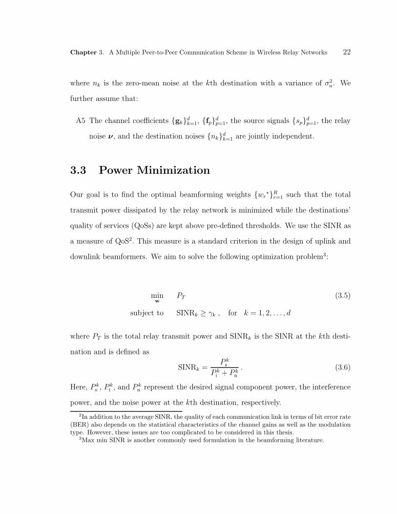
3.3 Power Minimization
Our goal is to find the optimal beamforming weights {wr∗}R
r=1 such that the total
transmit power dissipated by the relay network is minimized while the destinations’
quality of services (QoSs) are kept above pre-defined thresholds. We use the SINR as
a measure of QoS2. This measure is a standard criterion in the design of uplink and
downlink beamformers. We aim to solve the following optimization problem3:
minw
PT (3.5)
subject to SINRk ≥ γk , for k = 1, 2, . . . , d
where PT is the total relay transmit power and SINRk is the SINR at the kth desti-
nation and is defined as
SINRk =P k
s
P ki + P k
n
. (3.6)
Here, P ks , P k
i , and P kn represent the desired signal component power, the interference
power, and the noise power at the kth destination, respectively.
2In addition to the average SINR, the quality of each communication link in terms of bit error rate(BER) also depends on the statistical characteristics of the channel gains as well as the modulationtype. However, these issues are too complicated to be considered in this thesis.
3Max min SINR is another commonly used formulation in the beamforming literature.

Chapter 3. A Multiple Peer-to-Peer Communication Scheme in Wireless Relay Networks 23
We now derive the expressions for the total transmit power PT and SINRk. Using
(3.3), the total transmit power is given by
PT = E{tHt}
= E{xHWWHx
}
= tr{WHE
{xxH
}W}
(3.7)
Denoting the correlation matrix of the relay received signals by Rx , E{xxH}, we
rewrite the total transmit power as
PT = tr{WHRxW
}=
R∑
r=1
|wr|2[Rx]r,r = wHDw (3.8)
where w , diag(W) and D , diag([Rx]1,1, [Rx]2,2, · · · , [Rx]R,R). Note that using
(3.2) as well as Assumptions A1-A4, the matrix Rx is expressed as
Rx =d∑
p,q=1
E{fpf
Hq
}E{sps
∗q} + σ2
νI
=
d∑
p=1
PpE{fpf
Hp
}+ σ2
νI
=
d∑
p=1
PpRpf + σ2
νI (3.9)
where
Rpf , E
{fpf
Hp
}(3.10)
Note that the transmitted power PT depends not only on the variances of the
source-relay channel coefficients but also on the relay noise powers.
We now derive expressions for the desired signal component power P ks , the in-
terference power P ki , and the noise power P k
n in terms of {wr∗}R
r=1. Using (3.4) and
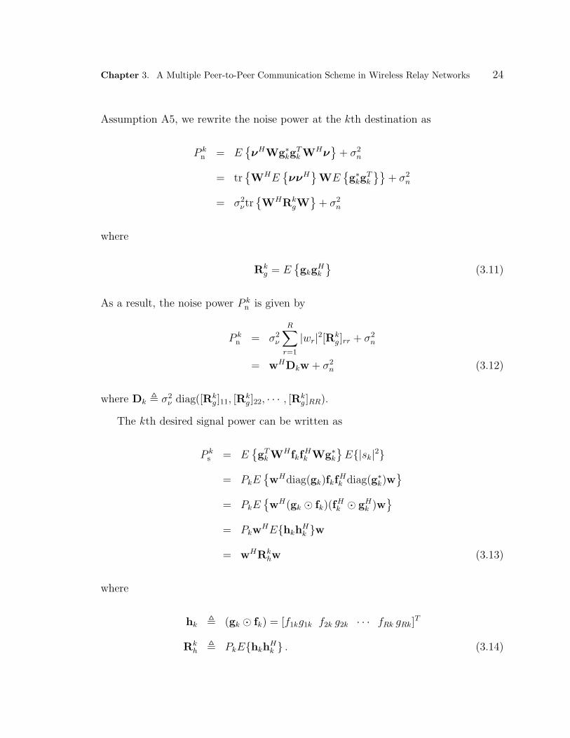
Chapter 3. A Multiple Peer-to-Peer Communication Scheme in Wireless Relay Networks 24
Assumption A5, we rewrite the noise power at the kth destination as
P kn = E
{ν
HWg∗kg
Tk WH
ν}
+ σ2n
= tr{WHE
{νν
H}
WE{g∗
kgTk
}}+ σ2
n
= σ2νtr{WHRk
gW}
+ σ2n
where
Rkg = E
{gkg
Hk
}(3.11)
As a result, the noise power P kn is given by
P kn = σ2
ν
R∑
r=1
|wr|2[Rkg ]rr + σ2
n
= wHDkw + σ2n (3.12)
where Dk , σ2ν diag([Rk
g ]11, [Rkg ]22, · · · , [Rk
g ]RR).
The kth desired signal power can be written as
P ks = E
{gT
k WHfkfHk Wg∗
k
}E{|sk|2}
= PkE{wHdiag(gk)fkf
Hk diag(g∗
k)w}
= PkE{wH(gk � fk)(f
Hk � gH
k )w}
= PkwHE{hkh
Hk }w
= wHRkhw (3.13)
where
hk , (gk � fk) = [f1kg1k f2k g2k · · · fRk gRk]T
Rkh , PkE{hkh
Hk } . (3.14)

Chapter 3. A Multiple Peer-to-Peer Communication Scheme in Wireless Relay Networks 25
It is worth mentioning that the vector hk contains the total path gains from the kth
source to its corresponding destination via different relays.
Denoting Dk = {1, 2, · · · , d} − {k} and using (3.4), the interference power at the
kth destination is given by
P ki = E
{
gTk WH
(∑
p,q∈Dk
fpfHq sps
∗q
)
Wg∗k
}
= E
{
wHdiag(gk)
(∑
p∈Dk
PpfpfHp
)
diag(g∗k)w
}
= E
{
wH
(∑
p∈Dk
Pp(gk � fp)(gHk � fH
p )
)
w
}
= wHE
{∑
p∈Dk
Pphpk(h
pk)
H
}
w
= wHQkw (3.15)
where hpk and Qk are defined as
hpk , gk � fp
Qk , E
{∑
p∈Dk
Pphpk(h
pk)
H
}
. (3.16)
The vector hpk contains the path coefficients from the pth source to the kth destination
via R relays.
Uisng (3.8), (3.12) (3.13), and (3.15), we rewrite the optimization problem in (3.5)
as
minw
wHDw (3.17)
subject towHRk
hw
wH(Qk + Dk)w + σ2n
≥ γk, for k = 1, 2, . . . , d .

Chapter 3. A Multiple Peer-to-Peer Communication Scheme in Wireless Relay Networks 26
Since wH(Qk + Dk)w + σ2n ≥ 0, the above problem is equivalent to
minw
wHDw (3.18)
subject to wH(Rkh − γk(Qk + Dk))w ≥ γkσ
2n, for k = 1, 2, . . . , d .
The problem in (3.18) is not a convex optimization problem and may not have a
solution with affordable computational complexity. We exploit a semi-definite relax-
ation approach to solve a relaxed version of (3.18). To do so, let us define X , wwH .
Then, the optimization problem in (3.18) can be rewritten as
minX
tr(DX) (3.19)
subject to tr(TkX) ≥ γkσ2n, for k = 1, 2, . . . , d
and rank (X) = 1, X � 0
where Tk , Rkh − γk(Qk + Dk). Only the rank constraint in (3.19) is not convex.
Using semi-definite relaxation, we remove this non-convex constraint and aim to solve
the following optimization problem
minX
tr(DX) (3.20)
subject to tr(TkX) ≥ γkσ2n , for k = 1, 2, . . . , d
and X � 0 .
The optimization problem (3.20) is indeed convex and can be solved efficiently
using interior point based software tools such as SeDuMi [36]. However, the matrix
Xopt, obtained by solving the optimization problem (3.20), is not necessarily of rank
one, and the minimum value of the relaxed problem (3.20) only provides a lower
bound on the minimum value of the original problem (3.18). Interestingly, it can be

Chapter 3. A Multiple Peer-to-Peer Communication Scheme in Wireless Relay Networks 27
shown that the semidefinite relaxation provides the same lower bound to the original
problem as the dual problem does (See Appendix A).
As it is shown in [13], we can always find a rank-one solution to the relaxed problem
(3.20) as long as d ≤ 3. Otherwise one might resort to randomization techniques to
obtain a suboptimal rank-one solution. In these techniques, the optimal matrix Xopt
is used to generate several suboptimal weight vectors, from which the best solution
will be selected [23, 35, 38, 39]. Surprisingly, in all our numerical simulations (except
for d = 4), the solution to the SDP problem turned out to be rank-one and hence its
principal eigenvector is the optimal solution to the original problem.
Introducing slack variables αk ≥ 0, for k = 1, ..., d, we can put the relaxed prob-
lem (3.20) into the standard SDP form [3]:
minX∈CR×R
vec(D)Tvec(X) (3.21)
subject to vec(Tk)T vec(X) − αk = γkσ
2n, for k = 1, 2, . . . , d,
αk ≥ 0, for k = 1, 2, . . . , d,
X � 0 .
The optimization problem (3.21) can now be efficiently solved using SeDuMi [36].
3.4 Individual Relay Power Constraints
In the previous section, we developed a computationally efficient technique for dis-
tributed multiplexing. This technique however does not guarantee that the relay
powers are distributed fairly. As a result some of the relays may end up with sig-
nificantly high transmit powers which is impractical due to power limitations of the
transmit amplifiers. In this section, we impose individual constraints on relay powers
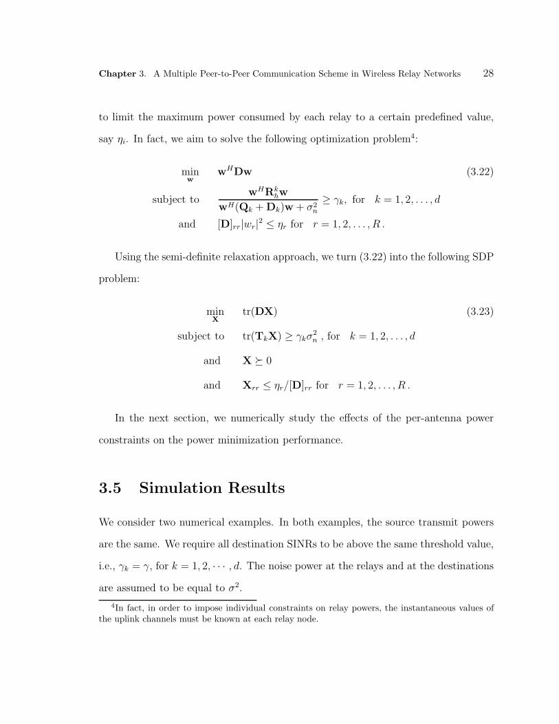
Chapter 3. A Multiple Peer-to-Peer Communication Scheme in Wireless Relay Networks 28
to limit the maximum power consumed by each relay to a certain predefined value,
say ηi. In fact, we aim to solve the following optimization problem4:
minw
wHDw (3.22)
subject towHRk
hw
wH(Qk + Dk)w + σ2n
≥ γk, for k = 1, 2, . . . , d
and [D]rr|wr|2 ≤ ηr for r = 1, 2, . . . , R .
Using the semi-definite relaxation approach, we turn (3.22) into the following SDP
problem:
minX
tr(DX) (3.23)
subject to tr(TkX) ≥ γkσ2n , for k = 1, 2, . . . , d
and X � 0
and Xrr ≤ ηr/[D]rr for r = 1, 2, . . . , R .
In the next section, we numerically study the effects of the per-antenna power
constraints on the power minimization performance.
3.5 Simulation Results
We consider two numerical examples. In both examples, the source transmit powers
are the same. We require all destination SINRs to be above the same threshold value,
i.e., γk = γ, for k = 1, 2, · · · , d. The noise power at the relays and at the destinations
are assumed to be equal to σ2.
4In fact, in order to impose individual constraints on relay powers, the instantaneous values ofthe uplink channels must be known at each relay node.

Chapter 3. A Multiple Peer-to-Peer Communication Scheme in Wireless Relay Networks 29
In the first example, we assume that all channel coefficients are exactly known at
a processing center where the beamforming weights for relays are to be determined.
This center then broadcasts the beamforming weights to the relays. In each simulation
run, the channel coefficients {frp} and {grp} are generated as i.i.d complex Gaussian
random variables with variances σ2f and σ2
g , respectively. As the channel coefficients
are known at the processing center, σ2f controls the quality of uplink channels from
the sources to the relays. Similarly, σ2g controls the quality of the downlink channels
from the relays to the destinations.
We first study the effect of the quality of the uplink and downlink channels on
the performance of the proposed scheme. To do so, we consider a network consisting
of 2 source-destination pairs and 20 relays. Fig. 3.2 shows the average minimum
power (normalized by the noise power σ2) consumed by all relaying nodes, versus
γ, for σ2g/σ
2 = 10 dB and for different values of σ2f/σ
2. In this figure, the average
minimum power is plotted only for those values of γ for which the beamforming
problem is feasible. From this figure, we observe that an improvement in the quality
of the uplink channels results in reduction of the average minimum power required to
satisfy a certain QoS at the destinations.
In Fig. 3.3, we have plotted the probability of having a feasible solution for the
distributed beamforming problem, for σ2g/σ
2 = 10 dB and for different values of σ2f/σ
2.
This figure clearly shows that it becomes more likely for the beamforming problem
to have a feasible solution as the quality of the uplink channels is improved. It is
interesting to observe that for every 5 dB increase in σ2f/σ
2, the feasibility probability
curves are shifted approximately by 5 dB to the right.

Chapter 3. A Multiple Peer-to-Peer Communication Scheme in Wireless Relay Networks 30
0 5 10 15 20 25−20
−15
−10
−5
0
5
10
15
20
25
30
σ2f/σ2 = −5 dB
σ2f/σ2 = 0 dB
σ2f/σ2 = 5 dB
σ2f/σ2 = 10 dB
σ2f/σ2 = 15 dB
Nor
mal
ized
aver
age
min
imum
pow
er(d
B)
Required SINR, γ (dB)
Figure 3.2: Normalized average minimum power versus SINR threshold γ, for σ2g/σ
2 =10 dB, and for different values of σ2
f/σ2, first example.
0 5 10 15 20 25 30 350
0.1
0.2
0.3
0.4
0.5
0.6
0.7
0.8
0.9
1
σ2f/σ2 = −5 dB
σ2f/σ2 = 0 dB
σ2f/σ2 = 5 dB
σ2f/σ2 = 10 dB
σ2f/σ2 = 15 dB
Pro
bab
ility
offe
asib
leso
luti
on
Required SINR, γ (dB)
Figure 3.3: Probability of feasible solution versus SINR threshold γ, for σ2g/σ
2 = 10dB, and for different values of σ2
f/σ2, first example.

Chapter 3. A Multiple Peer-to-Peer Communication Scheme in Wireless Relay Networks 31
0 2 4 6 8 10 12 14 16 18 20
−20
−10
0
10
20
30
40σ2
g/σ2 = −5 dB
σ2g/σ
2 = 0 dB
σ2g/σ
2 = 5 dB
σ2g/σ
2 = 10 dB
σ2g/σ
2 = 15 dBN
orm
aliz
edav
erag
em
inim
um
pow
er(d
B)
Required SINR, γ (dB)
Figure 3.4: Normalized average minimum power versus SINR threshold γ, for σ2f/σ
2 =10 dB, and for different values of σ2
g/σ2, first example.
0 5 10 15 20 25 300
0.1
0.2
0.3
0.4
0.5
0.6
0.7
0.8
0.9
1
σ2g/σ
2 = −5 dB
σ2g/σ
2 = 5 dB
σ2g/σ
2 = 15 dB
Pro
bab
ility
offe
asib
leso
luti
on
Required SINR, γ (dB)
Figure 3.5: Probability of feasible solution versus SINR threshold γ, for σ2f/σ
2 = 10dB, and for different values of σ2
g/σ2, first example.

Chapter 3. A Multiple Peer-to-Peer Communication Scheme in Wireless Relay Networks 32
Fig. 3.4 illustrates the normalized average minimum power, consumed by all re-
laying nodes, versus γ, for σ2f/σ
2 = 10 dB, and for different values of σ2g/σ
2. As can
be seen from Fig. 3.4, the higher the quality of the downlink channels, the lower the
average minimum power required to meet a certain QoS.
Fig. 3.5 illustrates the probability of the distributed beamforming problem having
a feasible solution versus γ for σ2f/σ
2 = 10 dB, and for different values of σ2g/σ
2.
We can see from this figure that the probability of feasible solution is invariant with
respect to the quality of the downlink channels quantified by σ2g/σ
2. This means that
the existence of a solution to the optimization problem (3.18) does not depend on
the quality of the downlink channels. This observation is justified by the fact that
in optimization problem (3.18), matrices Rkh, Qk, and Dk are all linear in σ2
g . Thus,
as σ2g decreases, the optimal solution w can be scaled up, thereby compensating for
the loss of quality of the downlink channels. This, in turn, results in scaling up the
objective function of (3.18), thereby increasing the total relay transmit power. This
explains why the total transmit power curves in Fig. 3.4 differ from each other by
exactly 5 dB steps as in these curves, σ2g/σ
2 changes in 5 dB steps.
We now study the effect of the number of relays. To do so, we consider different
number of relays serving 2 source-destination pairs. In this experiment, we choose
σ2f/σ
2 = σ2g/σ
2 = 10 dB. Figs. 3.6 and 3.7 show, respectively, the average minimum
power and the probability of having feasible solution versus SINR threshold γ for
different number of relays. These figures show that the higher the number of relays,
the lower the minimum relay power and the higher the probability of feasible solution
in order to meet a certain QoS measure.
To investigate the effect of the number of users on the performance of the network,

Chapter 3. A Multiple Peer-to-Peer Communication Scheme in Wireless Relay Networks 33
0 2 4 6 8 10 12 14 16 18 20 22−20
−15
−10
−5
0
5
10
15
20
25
10 relays20 relays30 relays
Nor
mal
ized
aver
age
min
imum
pow
er(d
B)
Required SINR, γ (dB)
Figure 3.6: Normalized average minimum power versus SINR threshold γ for differentnumber of relays, first example.
0 5 10 15 20 25 300
0.1
0.2
0.3
0.4
0.5
0.6
0.7
0.8
0.9
1
10 relays20 relays30 relays
Pro
bab
ility
offe
asib
leso
luti
on
Required SINR, γ (dB)
Figure 3.7: Probability of feasible solution versus SINR threshold γ for differentnumber of relays, first example.

Chapter 3. A Multiple Peer-to-Peer Communication Scheme in Wireless Relay Networks 34
0 2 4 6 8 10 12 14 16 18 20 22
−20
−15
−10
−5
0
5
10
15
20
25
1 user2 users3 users4 users
Nor
mal
ized
aver
age
min
imum
pow
er(d
B)
Required SINR, γ (dB)
Figure 3.8: Normalized average minimum power versus SINR threshold γ for differentnumber of source-destination pairs, first example.
0 5 10 15 20 25 300
0.1
0.2
0.3
0.4
0.5
0.6
0.7
0.8
0.9
1
1 user2 users3 users4 users
Pro
bab
ility
offe
asib
leso
luti
on
Required SINR, γ (dB)
Figure 3.9: Probability of feasible solution versus SINR threshold γ, for differentnumber of source-destination pairs, first example.
Chapter 3. A Multiple Peer-to-Peer Communication Scheme in Wireless Relay Networks 35
we consider four different networks which all consist of 20 relays but serve different
numbers of source-destination pairs for σ2f/σ
2 = σ2g/σ
2 = 10 dB. Figs. 3.8 and 3.9
show, respectively, the average minimum power and the probability of feasible solution
versus SINR threshold γ for different number of source-destination pairs. These
figures show that for a certain QoS measure γ, as the number of source-destination
pairs is increased, the minimum required relay power is increased, and the probability
of feasible solution is decreased.
It is however worth mentioning that these networks are using the wireless medium
for different network data rates. In other words, as the number of source-destination
pairs is increased, the data rate, which the network is supposed to support, is in-
creased. Therefore, it is a fair comparison to study the minimum relay power and the
probability of feasible solution for fixed network data rates. This is exactly where our
communication scheme can benefit from the spatial distribution of source-destination
pairs, and therefore, can outperform (semi-)orthogonal communication schemes such
as TDMA technique. To show this, we consider a network consisting of 4 source-
destination pairs and 20 relays. We study three different schemes as they are described
below.
• Scheme 1: We assume 8 different time slots, each with length T , are avail-
able for communication. In the first 4 time slots, the sources transmit their
data to the relays, using a TDMA scheme. In each of the remaining 4 time
slots, the relays transmit the beamformed version of the data they have re-
ceived from each source to the corresponding destination. In this scheme differ-
ent sources/destinations transmit/receive their data over temporally orthogonal
channels, and therefore, no interference exists among different links.

Chapter 3. A Multiple Peer-to-Peer Communication Scheme in Wireless Relay Networks 36
• Scheme 2: We assume 4 different time slots, each with length 2T , are available
for communication. Each time slot is used to set up a connection between two
source-destination pairs. In the first time slot, two sources transmit their data at
the same time. In the second time slot, the remaining two sources transmit their
data simultaneously. In the third time slot, the relays, transmit the amplitude
and phase-adjusted version of the data they have received during the first time
slot to the two destinations that correspond to the first two users. Finally, in
the last time slot, the relays transmit the beamformed version of the data they
have received in the second time slot toward the remaining two destinations.
• Scheme 3: We assume 2 time slots each with length 4T is available for commu-
nication. In the first time slot, all the four sources transmit their data toward
the relays. In the second time slot, the relays transmit the beamformed version
of the data they have received in the first time slot toward all 4 destinations.
In this case the interference is maximal among different pairs.
We assume that in scheme 2, the source transmit powers are half of the source
transmit powers in scheme 1. Taking into account that in scheme 2, the sources are
transmitting for a duration which is twice the period of the source transmission in
scheme 1, this will ensure that the average powers of scheme 1 and 2 are the same.
Similarly, we assume that in scheme 3, the source powers are a quarter of the source
powers in scheme 1. More specifically, the source transmit powers are 6 dB, 3 dB,
and 0 dB above the noise level for schemes 1, 2, and 3, respectively.
In this example, we assume that source-destination pairs are required to have
the same minimum data rate equal to D/d, where D is the network data rate. The
SINR threshold γ is obtained through the following relationship between the rate and

Chapter 3. A Multiple Peer-to-Peer Communication Scheme in Wireless Relay Networks 37
SINR5:
D
d= log(1 + γ) (3.24)
where d is the number of source-destination pairs which share the same time slot. That
is d is 1, 2, and 4 for schemes 1, 2, and 3, respectively. The so-obtained γ is then used
to obtain the beamforming weight vectors required in each scheme. Figs. 3.10 and
3.11 show, respectively, the normalized average minimum relay transmit power and
the probability of feasible solution versus minimum network data rate for the three
aforementioned schemes.
As can be seen from Fig. 3.10, as the minimum required network data rate is
increased, the relay transmit power can be decreased by increasing the number of
source-destination pairs which share the same time-slot6.
It is noteworthy that in scheme 1, one beamformer is needed per source-destination
pair. Therefore, the degrees of freedom (DoF) per destination is equal to the number
of relays which is 20 in this example. As a result, there are 80 DoF in this TDMA
network. Also, in scheme 1, only one QoS constraint is required per time slot. How-
ever, in scheme 3, only one beamformer is designed to cover all the four destinations
while four QoS constraints are to be satisfied. Hence, the total DoF for scheme 3
is 20 which a quarter of that for scheme 1. As a result, one expects that scheme 1
outperforms scheme 3 over the whole range of required network data rate.
However, one can see that beyond a certain value of D, scheme 3 outperforms
scheme 1. This phenomenon can be justified as it follows. For small values of data
rate D, the additional degrees of freedom offered by scheme 1 results in a better
5Here, we have assumed that the interference is Gaussian.6Only rank-one solutions have been considered in the case of d = 4. In almost 96 percent of our
simulation runs, the solution to the SDP problem is rank-one

Chapter 3. A Multiple Peer-to-Peer Communication Scheme in Wireless Relay Networks 38
0 0.5 1 1.5 2 2.5 3 3.5 4−30
−20
−10
0
10
20
30
scheme 1: 1 user per time slotscheme 2: 2 users per time slotscheme 3: 4 users per time slot
Nor
mal
ized
aver
age
min
imum
pow
er(d
B)
Minimum network data rate D (bits/sec/Hz)
Figure 3.10: Normalized average minimum transmit power versus network data rate,for three different schemes, for σ2
f = σ2g = 10 dB, first example.
0 0.5 1 1.5 2 2.5 3 3.5 40
0.1
0.2
0.3
0.4
0.5
0.6
0.7
0.8
0.9
1
scheme 1: 1 user per time slotscheme 2: 2 users per time slotscheme 3: 4 users per time slot
Pro
bab
ility
offe
asib
leso
luti
on
Minimum network data rate D (bits/sec/Hz)
Figure 3.11: Probability of feasible solution versus network data rate, for three dif-ferent schemes, for σ2
f = σ2g = 10 dB, first example.

Chapter 3. A Multiple Peer-to-Peer Communication Scheme in Wireless Relay Networks 39
0 5 10 15 20 25−20
−15
−10
−5
0
5
10
15
20
25
Unlimited relay powersLimited relay powers
Nor
mal
ized
aver
age
min
imum
pow
er(d
B)
Required SINR, γ (dB)
Figure 3.12: Normalized average minimum required transmit power versus SINRthreshold γ, with and without per relay power constraints, second example.
performance as compared to scheme 3. As D is increased, the QoS constraints become
increasingly difficult to satisfy. For scheme 1, we have that γ = 2D − 1, while for
scheme 3, γ = 2D/4 − 1 is chosen. Therefore, with the increase of D, the SINR
threshold for scheme 1 is increased much faster than that for scheme 3. This effect
overcomes the advantage of comparatively higher DoF offered by scheme 1. As a
result, the average minimum power for scheme 1 increases rapidly with increasing D
and the problem quickly becomes infeasible, while in scheme 3 the QoS constraints
are less stringent and the network can serve the source-destination connections for a
larger range of D. As can be seen from Fig. 3.11, scheme 3 remains feasible over a
larger range of D as compared to scheme 1. The performance of scheme 2 is between
those of schemes 1 and 3.
To consider the effect of per relay power constraint, we simulated a network with

Chapter 3. A Multiple Peer-to-Peer Communication Scheme in Wireless Relay Networks 40
0 5 10 15 20 250
0.1
0.2
0.3
0.4
0.5
0.6
0.7
0.8
0.9
1
Unlimited relay powersLimited relay powers
Pro
bab
ility
offe
asib
leso
luti
on
Required SINR, γ (dB)
Figure 3.13: Probability of feasible solution versus SINR threshold γ, with and with-out per relay power constraints, second example.
2 source-destination pairs and 20 relays. The maximum allowable power for each
relay is chosen to be 6 dB above the average power consumed by each relay in the
unconstrained problem. Also, the source powers were assumed to be 3 dB above the
noise power. We chose σ2f = σ2
g = 10 dB. Figs.3.12 and 3.13 illustrate, respectively,
the normalized average minimum power and the probability of feasible solution versus
SNR threshold γ.
As can be seen from these figures, such per-relay power constraints do not affect
the performance of our technique significantly for a wide range of γ up to 20 dB.
In our second numerical example, we assume that the second order statistics of
the channel coefficients (rather than their instantaneous values) are available. We
consider a network with R = 20 relay nodes. The channel coefficients frp and gr′q
are assumed to be independent from each other for any p, q, r, and r′. We also

Chapter 3. A Multiple Peer-to-Peer Communication Scheme in Wireless Relay Networks 41
0 0.5 1 1.5 2 2.5 3−20
−15
−10
−5
0
5
10
15
20
25
30
scheme 1: 1 user per time slotscheme 2: 2 users per time slotscheme 3: 4 users per time slot
Nor
mal
ized
aver
age
min
imum
pow
er(d
B)
Minimum network data rate D (bits/sec/Hz)
Figure 3.14: Normalized average minimum transmit power versus network data rateD, for three different schemes, for αf = −20 dB and αg = −10 dB, second example.
0 0.5 1 1.5 2 2.5 30
0.1
0.2
0.3
0.4
0.5
0.6
0.7
0.8
0.9
1
scheme 1: 1 user per time slotscheme 2: 2 users per time slotscheme 3: 4 users per time slot
Minimum network data rate D (bits/sec/Hz)
Pro
bab
ility
offe
asib
leso
luti
on
Figure 3.15: Probability of feasible solution versus network data rate, for three dif-ferent schemes, αf = −20 dB and αg = −10 dB, second example.

Chapter 3. A Multiple Peer-to-Peer Communication Scheme in Wireless Relay Networks 42
assume that the channel coefficient frp can be written as frp = frp + frp, where frp
is a known estimate of the channel coefficient frp and frp is a zero-mean random
variable which represents the estimation error. We assume that frp and fr′p are
independent for r 6= r′. We choose frp = ejθrp
√1 + αf
and var(frp) =αf
1 + αf, where θrp
is a uniform random variable chosen from the interval [0, 2π] and αf is a parameter
which determines the level of uncertainty in the channel coefficient frp. Note that
as E{|frp|2} = 1, if αf is increased, the variance of the random component frp is
increased while the mean value, frp is decreased. This, in turn, means that the level
of the uncertainty in the channel coefficient frp is increased. Similarly, we model the
channel coefficient grp as grp = grp + grp where grp is the known mean of grp and grp is
a zero-mean random variable. We assume that grp and gr′p are independent for r 6= r′.
We choose grp = ejφrp
√1 + αg
and var(grp) =αg
1 + αg, where φrp is a uniform random
variable chosen from the interval [0, 2π] and αg is a parameter which determines the
level of uncertainty in the channel coefficient grp. Based on this channel modeling,
we can write the (r, r′) entry of the matrices Rpf , Rk
g , Rkh, and Qk, respectively, as
Rpf(r, r
′) = (frpf∗r′p +
αf
1 + αf
δrr′)
Rkg(r, r
′) = (grkg∗r′k +
αg
1 + αgδrr′)
Rkh(r, r
′) = PkRkf(r, r
′)Rkg(r, r
′)
Qk(r, r′) =
d∑
p∈Dk
PpRpf(r, r
′)Rkg(r, r
′) .
Also, throughout this numerical example, the source transmit powers are 16, 13, and
10 dB above the noise level for schemes 1, 2, and 3, respectively, and αf = −20 dB and
αg = −10 dB. Figs. 3.14 and 3.15 illustrate the normalized average minimum power
and the probability of feasible solution, respectively, for the three aforementioned

Chapter 3. A Multiple Peer-to-Peer Communication Scheme in Wireless Relay Networks 43
schemes. As can be seen, in this example, scheme 3 outperforms the TDMA based
scheme 1.
Chapter 4
A Distributed Downlink
Beamforming Scheme in Wireless
Relay Networks
4.1 Introduction
In this chapter, we consider a wireless network of d source-destination pairs and
R relaying nodes. Each source communicates its data through the relay network.
Our goal is to establish wireless connections between each source and its respective
destination. Our cooperative scheme consists of (d + 1) steps. In the first d steps,
all sources transmit their data to the relay network in different time slots. So each
relay obtains a noisy faded version of each source signal. In the next step, each relay
multiplies each of its received signals by a complex weight, adds them all together and
retransmits the result in the last (d+1)th time slot. We assume that the second order
statistics of all communication channels are available. We aim to find the optimal
44

Chapter 4. A Distributed Downlink Beamforming Scheme in Wireless Relay Networks 45
b
b
b
b
b
b
b
Source 1
Source 2
Destination 1
Destination 2
f1
f2
g1
g2
1
2
R
3
Figure 4.1: A network of R relays and 2 source-destination pairs.
complex weights at the relays to minimize the total power dissipated by the relay
network, while meeting the QoS requirements at all destinations.
In contrast to those problems considered in the transmit (downlink) beamforming
literature [1, 35], where the signals intended for different users are exactly known at
the transmitting antennas, in our communication scheme, only noisy faded versions
of source signals are available at the relays. We show that using a semi-definite
relaxation approach [22], our power minimization problem can be turned into a semi-
definite programming (SDP) problem, and therefore, it can be solved using interior
point methods.
4.2 Problem Formulation
Consider a wireless network with d source-destination pairs and R relaying nodes,
as shown in Fig. 4.1. Each source in the network wishes to communicate with its

Chapter 4. A Distributed Downlink Beamforming Scheme in Wireless Relay Networks 46
corresponding destination via the relay network. However, we assume that there is
no direct link between any source and any destination. We consider a transmission
scheme which consists of d + 1 consecutive time slots. The d sources successively
transmit their data during the first d time slots, so their signals do not interfere with
each other at the relay nodes. The relay network is then responsible to deliver the
data to the respective destinations in the (d+1)th slot by implementing a distributed
downlink beamforming scheme.
Let frp denote the channel gain from the pth source to the rth relay and grp
represent the channel gain from the rth relay to the pth destination. These channel
gains are assumed to be fixed over the d + 1 transmission time slots. Then, the rth
relay received signal at time slot p denoted by xrp is given by
xrp = frpsp + νrp, (4.1)
where νrp is the rth relay noise in the time slot p and sp is the information symbol
transmitted by the pth source. Again, we use the following assumptions:
A1. The relay noise is spatially and temporally white, i.e., E{νrpν∗r′p′} = σ2
νδrr′δpp′,
where σ2ν is the relay noise power.
A2. The power of the pth source is Pp, i.e., E{|sp|2} = Pp.
A3. The symbols transmitted by sources are uncorrelated, that is E{sps∗q} = Ppδpq.
The vector of the relay signals received at time slot p is then given by
xp = fpsp + νp, (4.2)
where xp , [x1p x2p . . . xRp]T , νp , [ν1p ν2p . . . νRp]
T , and fp , [f1p f2p . . . fRp]T .

Chapter 4. A Distributed Downlink Beamforming Scheme in Wireless Relay Networks 47
The rth relay multiplies the signal received from the pth source by the complex
weight w∗rp, adds them up, and transmits the result to the destinations at the (d+1)th
time slot. Therefore, the R × 1 vector t of the signals transmitted by all relays is
expressed as
t =d∑
p=1
WHp (fpsp + νp) , (4.3)
where Wp , diag(wp), and wp , [w1p w2p . . . wRp]T is the pth beamforming weight
vector. Let us denote the vector of the channel gains from the relays to the kth
destination as gk , [g1k g2k . . . gRk]T .
The signal received at the kth destination is given by
yk = gkT t + nk
= gkT Wk
H fk sk︸ ︷︷ ︸
desired signal
+ gkT∑
p∈DK
WpHfpsp
︸ ︷︷ ︸
interference
+ gkT
d∑
p=1
WpH
νp + nk
︸ ︷︷ ︸
noise
, (4.4)
where nk is the zero-mean additive noise at the kth destination with a variance of σ2n
and Dk , {1, 2, . . . , d} − {k}. We make another assumption:
A4 The source signals {sp}dp=1, the relay noises {νp}d
p=1, the destination noises
{np}dp=1, and all channel gain vectors {gp}d
p=1 and {fp}dp=1 are statistically inde-
pendent.

Chapter 4. A Distributed Downlink Beamforming Scheme in Wireless Relay Networks 48
4.3 Power Minimization
In this section, we aim to find the relay weight vectors {wp}dp=1 such that the total
relay transmit power is minimized while maintaining the destinations’ quality of ser-
vices (QoSs) above pre-defined thresholds. Using the SINR as the measure of QoS,
our goal is to solve the following optimization problem:
minW
PT (4.5)
subject to SINRk ≥ γk , for 1 ≤ k ≤ d,
where W , {wp}dp=1 , PT is the total relay transmit power, and SINRk is the SINR
at the kth destination which is given by
SINRk =P k
s
P ki + P k
n
. (4.6)
Here, P ks , P k
i , and P kn are the desired signal power, the interference power, and the
noise power at the kth destination, respectively. Using (4.3) and assumptions A1-A4,
the total transmit power is written as
PT = E{tHt}
= E
{d∑
p,q=1
tr{Wp
HfpfqHWq
}sps
Hq
}
+ E
{d∑
p,q=1
tr{Wp
Hνpνq
HWq
}
}
=d∑
p=1
tr{Wp
H(PpR
pf + σ2
νI)Wp
}
=d∑
p=1
wpHDpwp, (4.7)

Chapter 4. A Distributed Downlink Beamforming Scheme in Wireless Relay Networks 49
where Dp , Pp(I � Rpf) + σ2
νI, Rpf , E
{fpf
Hp
}. The desired signal power at the kth
destination is given by
P ks = E
{gk
TWkHfkfk
HWkg∗k
}E{|sk|2}
= PkE{wk
HGkfkfkHGk
Hwk
}
= PkE{wk
H(fk � gk)(fk � gk)H)wk
}
= PkwkH(E{fkfkH} � E{gkgk
H})wk
= PkwHk
(Rk
f � Rkg
)wk, (4.8)
where Gk = diag(gk). It is worth mentioning that the rth entry of the vector fk � gk
is the total path gain between the kth source and its corresponding destination via
the rth relay (excluding the relay gains). Using (4.4) as well as assumptions A1-A4,
the interference power at the kth destination is written as
P ki = E
{
gkT
(∑
p,q∈Dk
WpHfpfq
HWqsps∗q
)
g∗k
}
= E
{∑
p∈Dk
PpwpHGkfpfp
HGkHwp
}
= E
{∑
p∈Dk
PpwpH(fp � gk)(f
Hp � gH
k )wp
}
=∑
p∈Dk
PpwpH(E{fpfpH} � E{gkgk
H})wp
=∑
p∈Dk
PpwpH(R
pf � Rk
g
)wp, (4.9)
where Rkg , E
{gkgk
H}. The vector fp � gk contains the total link gains from the
pth source to the kth destination that are passing through the R relays.

Chapter 4. A Distributed Downlink Beamforming Scheme in Wireless Relay Networks 50
Similarly the noise power at the kth destination is given by
Pn = E
{
gkT
(d∑
p,q=1
WpH
νpνqHWq
)
gk∗ + |nk|2
}
= σ2νE
{d∑
p=1
(gk
TWpHWpgk
∗)
}
+ σ2n
= σ2ν
d∑
p=1
wpH(I � E
{gkgk
H})
wp + σ2n
= σ2ν
d∑
p=1
wpH(I �Rk
g
)wp + σ2
n. (4.10)
Using (4.7), (4.8), (4.9), and (4.10), the optimization problem in (3.5) can be
rewritten as
minW
d∑
p=1
wpHDpwp (4.11)
subject to
d∑
p=1
wpHQkpwp ≥ γkσ
2n, for 1 ≤ k ≤ d,
where
Qkp ,
(PkRkf − γkσ
2νI) �Rk
g , if p = k
−γk(PpRpf + σ2
νI) �Rkg) , otherwise.
(4.12)
It is worth mentioning that at the optimum, all constraints hold with equality. Sup-
pose that a link SINR is higher than the predefined threshold, then we can scale
down the corresponding weight vector and hence decrease the total relay transmit
power without violating any constraints, which is a contradiction1. In general, the
optimization problem in (4.11) is not convex [3] and may not be amenable to a com-
putationally affordable solution. We propose to use the semi-definite relaxation to
1In fact, scaling down the weight vector corresponding to each user is beneficial to other source-destination pairs in the network because of less interference from that user.
Chapter 4. A Distributed Downlink Beamforming Scheme in Wireless Relay Networks 51
approximately solve (4.11). To do so, let us define Xp , wpwpH for 1 ≤ p ≤ d. In
this case, the problem in (4.11) becomes
minX
d∑
p=1
tr (XpDp) (4.13)
subject to
d∑
p=1
tr (XkQkp) ≥ γkσ2n
and rank (Xk) = 1, Xk � 0, for 1 ≤ k ≤ d,
where X , {Xp}dp=1. The rank constraints in (4.13) are not convex. We relax these
constraints and solve the following convex problem
minX
d∑
p=1
tr (XpDp) (4.14)
subject tod∑
p=1
tr (XkQkp) ≥ γkσ2n
and Xk � 0 , for 1 ≤ k ≤ d.
The optimization problem in (4.14) is convex and can be solved using interior
point based packages such as SeDuMi [36].
When using semi-definite relaxation, the solutions obtained by solving the relaxed
problem may not necessarily be of rank-one. However, as the following lemma implies,
we can always find a set of rank-one solutions {Xp}dp=1 to the relaxed problem (4.14).
Lemma 1 If the relaxed problem (4.14) is feasible, it always has at least one optimal
solution where all Xk are rank-one.
Lemma 1 can be proved following the guidelines of [1] when applied to our problem
(see Appendix B). In practice, the solution to the problem (4.14) always turns out
to be rank-one except for cases with exact symmetry. In this case, we can exploit
Lemma 5 in [1] to find a rank-one solution.

Chapter 4. A Distributed Downlink Beamforming Scheme in Wireless Relay Networks 52
4.4 Simulation Results
In our simulations we consider a network with 2 source-destination pairs and R = 10
relay nodes. The channel coefficient vectors fp and gq are assumed to be independent
from each other for any p and q. We also assume that the channel coefficient vector
fp can be written as fp = fp + fp, where fp is a known estimate of the channel vector
fp and fk is a zero-mean random vector which represents the estimation error.
We choose frp = ejθrp
√
1 + αf
and var(frp) =αf
1 + αf, where frp, and frp are the
rth entry of fp and fp, respectively, θrp is a uniform random variable chosen from the
interval [0 2π], and αf is a parameter which determines the level of uncertainty in the
channel coefficient frp. Note that as E{|frp|2} = 1, if αf is increased, the variance of
the random component of frp is increased while its mean is decreased. This, in turn,
means that the level of the uncertainty in the channel coefficient frp is increased.
Similarly, we model the channel coefficient gp as gp = gp + gp, where gp is the
(known) mean of gp, and gp is a zero-mean random vector with independent entries.
We choose grp = ejφrp
√
1 + αg
and var(grp) =αg
1 + αg, where grp and grp are the rth entry
of gp and gp, respectively, φrp is a uniform random variable chosen from the interval
[0 2π], and αg is a parameter which determines the level of uncertainty in the channel
coefficient grp. Based on this modeling, the matrices Rpf and Rp
g are respectively given
by
Rpf = fpf
Hp +
αf
1 + αfI
Rpg = gpg
Hp +
αg
1 + αgI
The relay and the destination noise powers are all assumed to be equal to 0 dBW,
i.e., σ2ν = σ2
n = 1. We require all destinations’ SINRs to be above the same threshold

Chapter 4. A Distributed Downlink Beamforming Scheme in Wireless Relay Networks 53
0 2 4 6 8 10 12 14 16 18 200
0.1
0.2
0.3
0.4
0.5
0.6
0.7
0.8
0.9
1
P/σ2n = 0 dB
P/σ2n = 5 dB
P/σ2n = 10 dB
P/σ2n = 15 dB
P/σ2n = 20 dB
P/σ2n = ∞ dB
SINR threshold γ (dB)
Pro
bab
ility
offe
asib
leso
luti
on
Figure 4.2: Probability of feasible solution versus SINR threshold, for different valuesof P/σ2
n, for αf = −20 dB and αg = −10 dB.
0 2 4 6 8 10 12 14 16 18 20−10
−5
0
5
10
15
20
25
30
35
40
P/σ2n = 0 dB
P/σ2n = 5 dB
P/σ2n = 10 dB
P/σ2n = 15 dB
P/σ2n = 20 dB
P/σ2n = ∞ dB
SINR threshold γ (dB)
Ave
rage
min
imum
rela
ytr
ansm
itpow
er(d
BW
)
Figure 4.3: Average minimum relay transmit power versus SINR threshold, for dif-ferent values of P/σ2
n, for αf = −20 dB and αg = −10 dB.
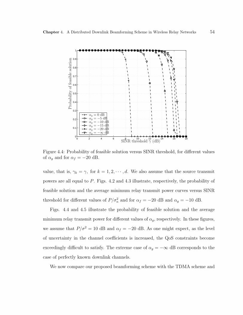
Chapter 4. A Distributed Downlink Beamforming Scheme in Wireless Relay Networks 54
0 2 4 6 8 10 12 14 16 180
0.1
0.2
0.3
0.4
0.5
0.6
0.7
0.8
0.9
1
αg = 0 dBαg = −5 dBαg = −10 dBαg = −15 dBαg = −20 dBαg = −∞ dB
SINR threshold γ (dB)
Pro
bab
ility
offe
asib
leso
luti
on
Figure 4.4: Probability of feasible solution versus SINR threshold, for different valuesof αg and for αf = −20 dB.
value, that is, γk = γ, for k = 1, 2, · · · , d. We also assume that the source transmit
powers are all equal to P . Figs. 4.2 and 4.3 illustrate, respectively, the probability of
feasible solution and the average minimum relay transmit power curves versus SINR
threshold for different values of P/σ2n and for αf = −20 dB and αg = −10 dB.
Figs. 4.4 and 4.5 illustrate the probability of feasible solution and the average
minimum relay transmit power for different values of αg, respectively. In these figures,
we assume that P/σ2 = 10 dB and αf = −20 dB. As one might expect, as the level
of uncertainty in the channel coefficients is increased, the QoS constraints become
exceedingly difficult to satisfy. The extreme case of αg = −∞ dB corresponds to the
case of perfectly known downlink channels.
We now compare our proposed beamforming scheme with the TDMA scheme and

Chapter 4. A Distributed Downlink Beamforming Scheme in Wireless Relay Networks 55
0 2 4 6 8 10 12 14 16−10
−5
0
5
10
15
20
25
30αg = 0 dBαg = −5 dBαg = −10 dBαg = −15 dBαg = −20 dBαg = −∞ dB
SINR threshold γ (dB)
Ave
rage
min
imum
rela
ytr
ansm
itpow
er(d
BW
)
Figure 4.5: Average minimum relay transmit power versus SINR threshold, for dif-ferent values of αg and for αf = −20 dB.
the communication scheme proposed in Chapter 3. Note that due to the amplify-and-
forward approach, different time slots have equal lengths and each source transmits
in only one time slot. Again we assume that the average source transmit powers are
the same. Again, if we assume that the interference is Gaussian, we can write
D =d
d + 1log(1 + γ) or
γ = 2(d+1)D
d − 1. (4.15)
where D is the total network data rate, and d is the number of sources transmitting at
the same time. In our simulations we consider a network with four source-destination
pairs and twenty relays. We assume that the relay and the destination noises are
Gaussian with the power of 0 dB and the average source powers are equal to 10 dB.
We also assume that αf and αg are equal to −20 dB. Fig. 4.6 and Fig. 4.7 illustrate

Chapter 4. A Distributed Downlink Beamforming Scheme in Wireless Relay Networks 56
100
101
0
0.1
0.2
0.3
0.4
0.5
0.6
0.7
0.8
0.9
1
Network data rate (bits/sec/Hz)
Prob
abili
ty o
f fe
asib
le s
olut
ion
Scheme 1Scheme 2Scheme 3
Figure 4.6: Probability of feasible solution versus network data rate.
the probability of feasible solution and the average minimum relay transmit-power
versus network data rate for three aforementioned schemes. Scheme 1, Scheme 2, and
Scheme 3 represent the orthogonal TDMA scheme and the proposed beamforming
schemes in Chapter 3 and 4, respectively. As can be seen from these figures, the
second scheme significantly outperforms the other two schemes when the required
data rate is high. Although the SINR threshold increases exponentially with the
data rate in all three schemes, the increase in γ is much slower for the second scheme.
This results in the better performance of the second scheme at high data rates. In the
third scheme, one beam is designed per destination, which results in higher degrees of
freedom and better performance over the other two schemes at low to medium data
rate. The first scheme is preferred when the complexity is the major concern.
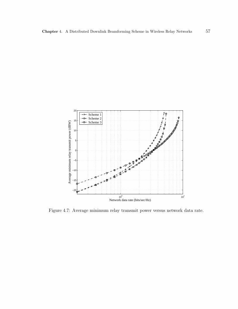
Chapter 4. A Distributed Downlink Beamforming Scheme in Wireless Relay Networks 57
100
101
−20
−15
−10
−5
0
5
10
15
20
Network data rate (bits/sec/Hz)
Ave
rage
min
imum
rel
ay tr
ansm
it po
wer
(dB
W)
Scheme 1Scheme 2Scheme 3
Figure 4.7: Average minimum relay transmit power versus network data rate.

Chapter 5
Conclusions and Future Work
Due to its simplicity, the amplify-and-forward approach has been widely studied in
the literature to gain better insight into cooperative communications. We proposed
two cooperative beamforming schemes to establish wireless connections between mul-
tiple source-destination pairs in a relay network. By exploiting the inherent spatial
diversity of wireless users, our proposed schemes result in a significant improvement
in the spectral efficiency of the wireless network.
In Chapter 3, we considered a network consisting of d source-destination pairs and
R relaying nodes. We studied the problem of multiple peer-to-peer communication
using an amplify-and-forward approach. In our scheme, first, the d sources transmit
their information symbols simultaneously to the relay network. Then, each relay
transmits an amplitude- and phase-adjusted version of its received signal. These
adjustments are made by multiplication of the relays’ received signal by a complex
weight. In this scheme, one beam covers all the destinations and mitigates the cross-
link interference. The optimal weight vector is in fact a receive and a transmit
beamformer at the same time. This vector is obtained through the minimization
58
Chapter 5. Conclusions and Future Work 59
of the total relay transmit power under quality of services constraints at all links.
We used semi-definite relaxation to convert this optimization problem into a semi-
definite programming problem and solved the resulting convex problem efficiently
using interior point methods. By exploiting the spatial diversity of sources, relays,
and destinations, our method allows multiple source-destination pairs to share the
available resources.
In Chapter 4, we studied the problem of distributed downlink beamforming in a
relay network where the relaying nodes cooperate to establish multiple peer-to-peer
communication links. Having the idea of downlink beamforming in mind, our goal
was to minimize the total power dissipated by the relay network subject to quality of
service constraints, measured by SINR, at the destination nodes. Our communication
scheme consists of two phases. In the first phase, the sources transmit their infor-
mation using a TDMA scheme. In the second phase, the relay nodes multiply their
received signals by complex weights, and thereby, build one beam per destination
collectively. We formulated the problem of relay transmit power minimization and
showed that it can be solved using a semi-definite relaxation approach.
We compared our proposed schemes with the conventional TDMA scheme in terms
of probability of feasible solution and average minimum relay transmit power. We
showed that the proposed schemes significantly outperform the TDMA scheme, spe-
cially, at high data rates.
However, optimal beamforming schemes result in more complexity as well as more
sensitivity to channel uncertainties. Furthermore, the assumption that all channel
statistics are available at a processing center may result in high system overhead.
Therefore, developing suboptimal beamforming schemes that are more robust and

Chapter 5. Conclusions and Future Work 60
require only local channel information is of particular interest for future research.
Another important question is how to best group the source-destination pairs
into cooperating groups and how to choose the best (possibly small) set of relays to
guarantee the QoS constraints, while keeping the complexity of the problem as low
as possible.

Bibliography
[1] M. Bengtsson and B. Ottersten. Optimal and suboptimal transmit beamforming.
In L. C. Godara, editor, Handbook of Antennas in Wireless Communications,
chapter 18. CRC Press, Boca Raton, FL, August 2001.
[2] M. Biguesh, S. Shahbazpanahi, and A. B. Gershman. Robust downlink power
control in wireless cellular systems. EURASIP Journal on Wireless Communi-
cations and Networking, 2004:261–272, December 2004.
[3] S. Boyd. Convex Optimization. Cambridge University Press, 2004.
[4] B. K. Chalise, S. Shahbazpanahi, A. Czylwik, and A. B. Gershman. Robust
downlink beamforming based on outage probability specifications. IEEE Trans-
actions on Wireless Communications, 6(10):3498–3503, October 2007.
[5] S. Fazeli-Dehkordy, S. Gazor, and S. Shahbazpanahi. Distributed peer-to-peer
multiplexing using ad hoc relay networks. Acoustics, Speech and Signal Process-
ing, 2008. IEEE International Conference on, pages 2373–2376, 2008.
[6] S. Fazeli-Dehkordy, S. Shahbazpanahi, and S. Gazor. Multiple peer-to-peer com-
munications using a network of relays. submitted to Signal Processing, IEEE
Transactions on, 2008.
61

Bibliography 62
[7] M.R. Garey and D.S. Johnson. Computers and Intractability: A Guide to the
Theory of NP-Completeness. WH Freeman & Co. New York, NY, USA, 1979.
[8] A. Goldsmith. Wireless Communications. Cambridge University Press, 2005.
[9] D. Hammarwall, M. Bengtsson, and B. Ottersten. On downlink beamforming
with indefinite shaping constraints. Signal Processing, IEEE Transactions on,
54(9):3566–3580, September 2006.
[10] I. Hammerstrom, M. Kuhn, and A. Wittneben. Impact of relay gain allocation
on the performance of cooperative diversity networks. In Proc. The IEEE 60th
Vehicular Technology Conference, Fall 2004., volume 3, pages 1815–1819, Los
Angeles, CA, September 2004.
[11] V. Havary-Nassab, S. Shahbazpanahi, A. Grami, and Z.-Q. Luo. Distributed
beamforming for relay networks based on second order statistics of the channel
state information. Signal Processing, IEEE Transactions on, 2008, to appear,
see also Proc. ICASSP 2008.
[12] Y.-W. Hong, W.-J. Huang, F.-H. Chiu, and C.-C. J. Kuo. Cooperative com-
munications in resource-constrained wireless networks. IEEE Signal Processing
Magazine, 24:47–57, 2007.
[13] Y. Huang and S. Zhang. Complex Matrix Decomposition and Quadratic Pro-
gramming. Mathematics of Operations Research, 32(3):758, 2007.
[14] M. Janani, A. Hedayat, T. E. Hunter, and A. Nosratinia. Coded cooperation in
wireless communications: space-time transmission and iterative decoding. Signal
Processing, IEEE Transactions on, 52:362–371, February 2004.
Bibliography 63
[15] Y. Jing and B. Hassibi. Distributed space-time coding in wireless relay networks.
IEEE Transactions on Wireless Communications, 5(12):3524–3536, 2006.
[16] Y. Jing and H. Jafarkhani. Network beamforming using relays with perfect
channel information. In Proc. The IEEE International Conference on Acoustics,
Speech and Signal Processing, volume 3, Honolulu, HI, April 2007.
[17] Y. Jing and H. Jafarkhani. Distributed differential space-time coding for wireless
relay networks. Communications, IEEE Transactions on, 56(7):1092–1100, 2008.
[18] Y. Jing and H. Jafarkhani. Network beamforming using relays with perfect
channel information. Submitted, Dec. 2006.
[19] G. Kramer, M. Gastpar, and P. Gupta. Cooperative Strategies and Capac-
ity Theorems for Relay Networks. Information Theory, IEEE Transactions on,
51(9):3037–3063, 2005.
[20] J. N. Laneman, D. N. C. Tse, and G. W. Wornell. Cooperative diversity in
wireless networks: Efficient protocols and outage behavior. Information Theory,
IEEE Transactions on, 50:3062–3080, December 2004.
[21] J. N. Laneman and G. W. Wornell. Distributed space-time-coded protocols for
exploiting cooperative diversity in wireless networks. Information Theory, IEEE
Transactions on, 49:2415–2425, October 2003.
[22] Z. Q. Luo and W. Yu. An introduction to convex optimization for communica-
tions and signal processing. IEEE Journal on Selected Areas in Communications,
24:1426–1438, August 2006.

Bibliography 64
[23] W.-K. Ma, T. N. Davidson, K. M. Wong, Z.-Q. Luo, and P.-C. Ching. Quasi-
maximum-likelihood multiuser detection using semi-definite relaxation with ap-
plication to synchronous CDMA. Signal Processing, IEEE Transactions on,
50:912–922, April 2002.
[24] C.D. Meyer. Matrix Analysis and Applied Linear Algebra. Society for Industrial
Mathematics, 2000.
[25] A.L. Moustakas, S.H. Simon, and A.M. Sengupta. MIMO capacity through
correlated channels in the presence of correlated interferers and noise: a (not so)
large N analysis. Information Theory, IEEE Transactions on, 49(10):2545–2561,
2003.
[26] R. U. Nabar, H. Bolcskei, and F. W. Kneubuhler. Fading relay channels: per-
formance limits and space-time signal design. IEEE Journal on Selected Areas
in Communications, 22:1099–1109, August 2004.
[27] A. Nosratinia, TE Hunter, and A. Hedayat. Cooperative communication in
wireless networks. Communications Magazine, IEEE, 42(10):74–80, 2004.
[28] F. Rashid-Farrokhi, K. J. R. Liu, and L. Tassiulas. Transmit beamforming and
power control for cellular wireless systems. IEEE Journal on Selected Areas in
Communications, 16(8):1437–1450, October 1998.
[29] F. Rashid-Farrokhi, KJR Liu, and L. Tassiulas. Downlink power control and
base station assignment. Communications Letters, IEEE, 1(4):102–104, 1997.

Bibliography 65
[30] F. Rashid-Farrokhi, L. Tassiulas, and KJR Liu. Joint optimal power control and
beamforming in wireless networksusing antenna arrays. Communications, IEEE
Transactions on, 46(10):1313–1324, 1998.
[31] M. Schubert and H. Boche. Solution of the multiuser downlink beamforming
problem with individual SINR constraints. Vehicular Technology, IEEE Trans-
actions on, 53(1):18–28, January 2004.
[32] M. Schubert and H. Boche. Iterative multiuser uplink and downlink beamforming
under SINR constraints. Signal Processing, IEEE Transactions on, 53(7):2324–
2334, July 2005.
[33] A. Sendonaris, E. Erkip, and B. Aazhang. User cooperation diversity-part I:
System description. Communications, IEEE Transactions on, 51:1927–1938,
November 2003.
[34] A. Sendonaris, E. Erkip, and B. Aazhang. User cooperation diversity-part II: Im-
plementation aspects and performance analysis. Communications, IEEE Trans-
actions on, 51:1939–1948, November 2003.
[35] N. D. Sidiropoulos, T. N. Davidson, and Z.-Q. Luo. Transmit beamforming for
physical-layer multicasting. Signal Processing, IEEE Transactions on, 54:2239–
2251, June 2006.
[36] J. F. Sturm. Using SeDuMi 1.02, a Matlab toolbox for optimization over sym-
metric cones. Optimization Methods and Software, 11-12:625–653, 1999.
[37] D. Tse and P. Viswanath. Fundamentals of Wireless Communication. Cambridge
University Press, 2005.

Bibliography 66
[38] P. Tseng. Further results on approximating nonconvex quadratic optimization
by semidefinite programming relaxation. SIAM J. Optim., 14(1):268–283, jul
2003.
[39] S. Zhang. Quadratic maximization and semidefinite relaxation. Math. Program.,
87:453–465, 2000.
[40] Y. Zhao and R. Adve. Improving amplify-and-forward relay networks: Optimal
power allocation versus selection. In Proc. IEEE International Symposium on
Information Theory,, pages 1234–1238, Seattle, WA, July 2006.
[41] L. Zheng and D. N. C. Tse. Diversity and multiplexing: a fundamental trade-
off in multiple-antenna channels. Information Theory, IEEE Transactions on,
49(5):1073–1096, May 2003.
Appendix A
Semidefinite Relaxation and The
Duality Gap
We further explore the relationship between the original problem (3.18) and the re-
laxed problem (3.20). The Lagrangian of the optimization problem (3.18) can be
written as
L(w, λ) = wHDw +
d∑
k=1
λk(γkσ2n − wHTkw)
= wH
(
D −d∑
k=1
λkTk
)
w +
d∑
k=1
λkγkσ2n (A.1)
where {λk}dk=1 are the non-negative dual variables and λ , [λ1 λ2 . . . , λd]
T . There-
fore, the corresponding dual objective function is given by
g(λ) = minw∈CR
L(w, λ) . (A.2)
67

Appendix A. Semidefinite Relaxation and The Duality Gap 68
It is easy to show that the quadratic term in (A.1) is unbounded from below unless
D −∑dk=1
λkTk � 0. Hence, the dual problem is
maxλ<0
d∑
k=1
γkσ2nλk (A.3)
subject to D −d∑
k=1
λkTk � 0
λk ≥ 0, for k = 1, 2, . . . , d .
It can be easily shown that the dual of the relaxed problem in (3.20) is exactly the
same as (A.3). This means that the dual problems for both the original problem (3.18)
and the relaxed problem (3.20) are the same. Since the maximum value of the dual
problem provides a lower bound for the minimum value of the original problem, the
maximum value of (A.3) is a lower bound for both optimal values of (3.18) and (3.20).
On the other hand, because the strong duality holds for the relaxed problem [3], [22],
the minimum value of (3.20) is the same as the maximum value of (A.3). Therefore,
we conclude that the semidefinite relaxation provides the same lower bound to the
original problem as the dual problem does. That is the gap between (3.18) and (3.20)
is equal to the duality gap.

Appendix B
Proof of Lemma 1
To prove Lemma 1, we need to introduce some new notations. We define
Rk,p = D−H/2p QkpD
−1/2p , (B.1)
and
D1/2p wp =
√zpup, zp ≥ 0 for 1 ≤ p ≤ d, (B.2)
where zp is a non negative scaler and up is a unit vector for 1 ≤ p ≤ d. The
optimization problem (4.11) can be rewritten in the form
mind∑
p=1
zpupHup
subject to ukH(zkRk,k
)uk +
∑
p 6=k
upH(zpRk,p
)up
−γkσ2n ≥ 0, for 1 ≤ k ≤ d, (B.3)
69
Appendix B. Proof of Lemma 1 70
and if we let Up = zpupupH , the relaxed problem (4.14) is written as
min
d∑
p=1
tr (Up)
subject to tr(Rk,kUk
)+∑
p 6=k
tr(Rk,pUp
)
−γkσ2n ≥ 0, and Uk � 0, for 1 ≤ k ≤ d. (B.4)
First, we provide some useful lemmas.
Lemma 2 The Lagrangian dual problem for the relaxed problem (B.4) is given by
maxλp
d∑
p=1
λpγpσ2n
subject to I − λkRk,k −∑
p 6=k
λpRp,k � 0
for 1 ≤ k ≤ d. (B.5)
Proof: The Lagrangian of the optimization problem (B.4) is given by
L (U , λ) =d∑
p=1
tr (Up) +d∑
k=1
λkγkσ2n
−d∑
k=1
λktr(Rk,kUk
)−
d∑
k=1
∑
p 6=k
λktr(Rk,pUp
), (B.6)
where U , {Up � 0}dp=1 and λ = [λ1, . . . , λd]
T . It can be written as
L (U , λ) =
d∑
p=1
λpγpσ2n +
d∑
k=1
tr (Uk)
−d∑
k=1
λktr(Rk,kUk
)−
d∑
k=1
∑
p 6=k
λptr(Rp,kUk
), (B.7)

Appendix B. Proof of Lemma 1 71
or
L (U , λ) =
d∑
p=1
λpγpσ2n
+
d∑
k=1
tr
(
(I − λkRk,k −∑
p 6=k
λpRp,k)Uk
)
(B.8)
The Lagrange dual function is written as
g(λ) = infU
L (U , λ) (B.9)
The term in (B.8) is unbounded from below unless we have
I − λkRk,k −∑
p 6=k
λpRp,k � 0
for 1 ≤ k ≤ d. (B.10)
Hence, the Lagrangian dual problem for the relaxed problem (B.4) is given by
maxλp
d∑
p=1
λpγpσ2n
subject to I − λkRk,k −∑
p 6=k
λpRp,k � 0
for 1 ≤ k ≤ d. (B.11)
Lemma 3 The following problems have the same optimal cost function and the same
optimal vector λ.
min
d∑
p=1
λpupHup
subject to ukH(λkRk,k
)uk +
∑
p 6=k
upH(λpRk,p
)up
−γkσ2n ≥ 0, for 1 ≤ k ≤ d. (B.12)
Appendix B. Proof of Lemma 1 72
mind∑
k=1
λkγkσ2n
subject to I − λpRp,p −∑
k 6=p
λkRk,p � 0
and λp ≥ 0, for 1 ≤ p ≤ d. (B.13)
Proof: If we define
[A]k,p = upHRk,pup (B.14)
the optimization problem (B.12) becomes
min λT ω
subject to Aλ = b
λp ≥ 0 (B.15)
‖up‖ = 1 for 1 ≤ p ≤ d,
where
ω =[‖u1‖2, . . . , ‖ud‖2
]T, (B.16)
b =[γ1σ
2n, . . . , γdσ
2n
]T. (B.17)
We can write A = A1 − A2 where
[A1]k,p =
ukHRk,kuk p = k
0 p 6= k
(B.18)
[A2]k,p = −upHRk,pup (B.19)

Appendix B. Proof of Lemma 1 73
For any matrix A satisfying the constraints in (B.15) we have
Aλ = b, (B.20)
(A1 −A2) λ = b, (B.21)
(I − A1
−1A2
)λ = A1
−1b, (B.22)
λp =[A1
−1b]
p+[A1
−1A2λ]
p> 0, (B.23)
[A1
−1A2λ]
p
λp= 1 −
[A1
−1b]
p
λp< 1. (B.24)
From Collatz-Wielandt formula (see [24]) we have
r(A1
−1A2
)≤ max
1≤p≤d
[A1
−1A2λ]
p
λp< 1. (B.25)
where r denotes the spectral radius of a matrix. From Perron-Frobenius theorem for
irreducible non-negative matrices and because the spectral radius of matrix A1−1A2
is less than 1 (see [24]), we conclude that(I − A1
−1A2
)−1exists and is non-negative.
So we can write
A−1 =(A1
(I −A−1
1 A2
))−1=(I − A−1
1 A2
)−1A−1
1 . (B.26)
Hence, A−1 also exists and is non-negative. So we can solve for λ:
λ = A−1b =(I − A−1
1 A2
)−1A−1
1 b. (B.27)
The optimization problem (B.15) can be rewritten as
min bT A−T1
subject to Aλ = b
λp ≥ 0 (B.28)
‖up‖ = 1 for 1 ≤ p ≤ d.

Appendix B. Proof of Lemma 1 74
On the other hand, for any invertible matrix A with non-negative inverse we can
always find λ ≥ 0 such that Aλ = b. Thus we can replace the first and the second
constraint in (B.28) to write it as
min bTA−T1
subject to A ∈ A (B.29)
‖up‖ = 1.
where A denotes the set of invertible matrices with non-negative inverse. Following
the above discussion, we can rewrite (B.29) as
min bT A−T1
subject to ATλ = 1
λp ≥ 0 (B.30)
‖up‖ = 1 for 1 ≤ p ≤ d,
or equivalently
min
d∑
k=1
λkγkσ2n
subject to upH
(
I − λpRp,p −∑
k 6=p
λkRk,p
)
up = 0
λp ≥ 0 (B.31)
‖up‖ = 1 for 1 ≤ p ≤ d.
Appendix B. Proof of Lemma 1 75
We can rewrite problem (B.31) as
min
d∑
k=1
λkγkσ2n
subject toup
HλpRp,pup
1 −∑k 6=p λkupHRk,pup
= 1
λp ≥ 0 (B.32)
‖up‖ = 1 for 1 ≤ p ≤ d,
which is a virtual uplink problem except for the weight factors γkσ2n. The first d
constraints are QoS requirements at the base station, one for each user. Note that
we can relax the QoS constraints in (B.32) to obtain
min
d∑
k=1
λkγkσ2n
subject toup
HλpRp,pup
1 −∑k 6=p λkupHRk,pup
≥ 1
λp ≥ 0 (B.33)
‖up‖ = 1 for 1 ≤ p ≤ d.
This is due to the fact that the SINR constraint for each user is always met with
equality at the optimum. Otherwise, the transmit power at the corresponding user
can be reduced without violating any constraint. This results in a lower cost function,
which is a contradiction. According to this argument, we can relax the problem (B.31)

Appendix B. Proof of Lemma 1 76
to obtain
mind∑
k=1
λkγkσ2n
subject to upH
(
I − λpRp,p −∑
k 6=p
λkRk,p
)
up ≤ 0
λp ≥ 0 (B.34)
‖up‖ = 1 for 1 ≤ p ≤ d,
which can be written as
mind∑
k=1
λkγkσ2n
subject to I − λpRp,p −∑
k 6=p
λkRk,p � 0
λp ≥ 0 (B.35)
‖up‖ = 1 for 1 ≤ p ≤ d.
Lemma 4 Problems (B.11) and (B.35) have the same optimal solution λ∗.
Proof: First we show that the optimal solution to problem (B.11) is a feasible solution
to problem (B.35) and vice versa. If we assume that the matrix in the kth constraint
in Problem (B.35) has some negative eigenvalues at the optimum, then we can reduce
the cost function by decreasing λk without violating any of the constraints, which
is a contradiction. Similarly, if we assume that the matrix in the kth constraint in
Problem (B.11) has only positive eigenvalues at the optimum, then we can increase
the objective function by increasing λk while satisfying all the constraints, which is
again a contradiction.

Appendix B. Proof of Lemma 1 77
Now we assume that both λ1 and λ
2 satisfy the constraints in both (B.11) and
(B.35). Without loss of generality, we assume that there exists an index k and a
constant α ≥ 1 such that λ1k = αλ2
k and λ1 ≤ αλ
2. From the kth constraint in (B.11)
we have:
αλ2kRk,k = λ1
kRk,k � I −∑
p 6=k
λ1pRp,k
� I −∑
p 6=k
αλ2pRp,k ≺ α(I−
∑
p 6=k
λ2pRp,k) (B.36)
which contradicts that λ2 satisfies the kth constraint in (B.35). Therefore, only a
single point satisfies all the constraints in (B.11) and (B.35) which is the optimal
solution to both problems.
Proof of Lemma 1: As it is shown in Lemma 4, the optimal solution of the
Lagrangian dual of the relaxed problem (B.11) is the same as the optimal solution of
(B.35), which is algebraically equivalent to the original problem (B.12), as a result of
Lemma 3. The dual problem always provides a lower bound for the relaxed problem
which in turn provides a lower bound for the original problem. Consequently all three
problems have the same optimal solution that results in the following fact: whenever
the problem (4.14) is feasible, there is at least one rank-one solution.