Distributed Architecture for Real-Time

Coordination in Transit Networks

Final Report

Metrans Project 00-13

July 2003

Satish Bukkapatnam

Maged Dessouky

Jiamin Zhao

Department of Industrial and Systems Engineering

University of Southern California

Los Angeles, CA 90089-0193

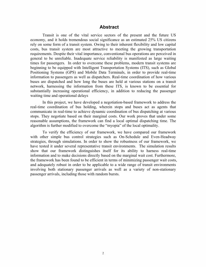
Disclaimer The contents of this report reflect the views of the authors, who are responsible

for the facts and the accuracy of the information presented herein. This document is disseminated under the sponsorship of the Department of Transportation, University Transportation Centers Program, and California Department of Transportation in the interest of information exchange. The U.S. Government and California Department of Transportation assume no liability for the contents or use thereof. The contents do not necessarily reflect the official views or policies of the State of California or the Department of Transportation. This report does not constitute a standard, specification, or regulation.

1

Abstract Transit is one of the vital service sectors of the present and the future US

economy, and it holds tremendous social significance as an estimated 25% US citizens rely on some form of a transit system. Owing to their inherent flexibility and low capital costs, bus transit system are most attractive to meeting the growing transportation requirements. Despite their vital importance, conventional bus operations are perceived in general to be unreliable. Inadequate service reliability is manifested as large waiting times for passengers. In order to overcome these problems, modern transit systems are beginning to be equipped with Intelligent Transportation Systems (ITS), such as Global Positioning Systems (GPS) and Mobile Data Terminals, in order to provide real-time information to passengers as well as dispatchers. Real-time coordination of how various buses are dispatched and how long the buses are held at various stations on a transit network, harnessing the information from these ITS, is known to be essential for substantially increasing operational efficiency, in addition to reducing the passenger waiting time and operational delays

In this project, we have developed a negotiation-based framework to address the real-time coordination of bus holding, wherein stops and buses act as agents that communicate in real-time to achieve dynamic coordination of bus dispatching at various stops. They negotiate based on their marginal costs. Our work proves that under some reasonable assumptions, the framework can find a local optimal dispatching time. The algorithm is further modified to overcome the “myopia” of the local optimality.

To verify the efficiency of our framework, we have compared our framework with other simple bus control strategies such as On-Schedule and Even-Headway strategies, through simulations. In order to show the robustness of our framework, we have tested it under several representative transit environments. The simulation results show that our framework distinguishes itself for its ability to harness real-time information and to make decisions directly based on the marginal wait cost. Furthermore, the framework has been found to be efficient in terms of minimizing passenger wait costs, and adequately robust in order to be applicable to a wide range of transit environments involving both stationary passenger arrivals as well as a variety of non-stationary passenger arrivals, including those with random bursts.

2

Table of Contents DISCLAIMER ............................................................................................................................................... 1

ABSTRACT .................................................................................................................................................. 2

TABLE OF CONTENTS ............................................................................................................................. 3

LIST OF FIGURES ...................................................................................................................................... 5

1. INTRODUCTION ..................................................................................................................................... 6

1.1 Background..................................................................................................................................... 6 1.1.1 Problem and Its Significance.................................................................................................................... 6 1.1.2 Approach and Impact ............................................................................................................................... 6 1.1.3 Relevance to ITS and Transit Research.................................................................................................... 7

1.2 Research Objectives........................................................................................................................ 7

2. LITERATURE REVIEW.......................................................................................................................... 9

2.1 Stationary Models ........................................................................................................................... 9 2.1.1 Headway-Based Strategies ....................................................................................................................... 9 2.1.2 Schedule-Based Strategies ..................................................................................................................... 10

2.2 Simulation Models ........................................................................................................................ 10 2.3 Real-Time Models ......................................................................................................................... 11

2.3.1 Traditional Works .................................................................................................................................. 11 2.3.2 Recent Trends to MAS Applications...................................................................................................... 11

3. RESEARCH METHODOLOGY........................................................................................................... 13

3.1 Problem Formulation.................................................................................................................... 13 3.1.1 The Transit Network .............................................................................................................................. 13 3.1.2 Objective Functions ............................................................................................................................... 13

3.2 Multi-Agent Framework................................................................................................................ 14 3.2.1 Architecture............................................................................................................................................ 14 3.2.2 Negotiation............................................................................................................................................. 14

3.3 Local Optimality Conditions......................................................................................................... 16 3.4 Hyperopic Considerations ............................................................................................................ 17

4. SIMULATION – STATIONARY PASSENGER ARRIVALS ........................................................... 20

4.1 Basic Settings ................................................................................................................................ 20 4.1.1 Physical Parameters ............................................................................................................................... 20 4.1.2 Set of Strategies...................................................................................................................................... 20

4.2 Simulation Results......................................................................................................................... 20 4.2.1 Scenario 1 – Straight Line with Different Scheduled Headways............................................................ 20 4.2.2 Scenario 2 – Loop with Different Scheduled Headways ........................................................................ 21

5. SIMULATION – NON-STATIONARY PASSENGER ARRIVALS ................................................. 24

5.1 Passenger Arrivals in Bursts......................................................................................................... 24 5.1.1 Physical Parameters ............................................................................................................................... 24 5.1.2 Set of Strategies...................................................................................................................................... 25 5.1.3 Scenario 1 – Effect of Different Passenger Average Arrival Rates (λ) ................................................. 25

5.1.4 Scenario 2 – Effect of Different Variances ( ) ................................................................................ 26 2pσ

5.1.5 Scenario 3 – Different Scheduled Headways ......................................................................................... 26 5.2 Passenger Arrivals with Awareness of Schedule .......................................................................... 27

5.2.1 Passenger Arrivals.................................................................................................................................. 27 5.2.2 Simulation Result ................................................................................................................................... 28

6. CONCLUSION....................................................................................................................................... 30

3

7. IMPLEMENTATION.............................................................................................................................. 31

REFERENCES ........................................................................................................................................... 32

APPENDIX 1 .............................................................................................................................................. 34

4

List of Figures FIGURE 3.1 TRANSIT NETWORK STRUCTURE IN OUR WORK ......................................................................... 13

FIGURE 3.2 MAS ARCHITECTURE ................................................................................................................. 14

FIGURE 3.3 OPTIMALITY CONDITION FOR NEGOTIATION BASED ON MARGINAL COST ................................. 17

FIGURE 4.1 SAVINGS OF DIFFERENT STRATEGIES VS. NO-WAIT STRATEGY.................................................. 21

FIGURE 4.3 COEFFICIENT OF VARIATION OF HEADWAYS OF DIFFERENT STRAEGIES AT EACH STOP............. 22

FIGURE 4.4 AVERAGE HEADWAYS OF DIFFERENT STATEGIES AT EACH STOP............................................... 23

FIGURE 5.1 PASSENGER ARRIVAL RATE WITH RANDOM BURSTS.................................................................. 24

FIGURE 5.2 SAVINGS OF DIFFERENT STRATEGIES UNDER DIFFERENT PASSENGER AVERAGE ARRIVAL RATES............................................................................................................................................................ 25

FIGURE 5.3 SAVINGS OF DIFFERENT STRATEGIES UNDER DIFFERENT ................................................... 26 2pσ

FIGURE 5.4 SAVINGS OF DIFFERENT STRATEGIES UNDER DIFFERENT HEADWAYS........................................ 27

FIGURE 5.5 P.D.F OF PASSENGER ARRIVAL TIME BASED ON UTILITY THEORY............................................. 28

FIGURE 5.6 PERFORMANCE COMPARING OF DIFFERENT STRATEGIES WITH AWARE PASSENGERS ................ 29

FIGURE 7.1 BASIC HARDWARE ENVIRONMENT FOR OUR PROPOSED FRAMEWORK....................................... 31

5

1. Introduction

1.1 Background

1.1.1 Problem and Its Significance

Transit is one of the vital service sectors of the present and the future US economy, and it holds tremendous social significance as an estimated 25% US citizens rely on some form of a transit system. Transit systems are essential for preserving and revitalizing the nation’s cities by minimizing congestion, urban sprawl, central city decline, and air pollution. Owing to their inherent flexibility and low capital costs, bus transit systems, in particular, are attractive to meeting the growing transportation requirements.

Despite these inherent advantages, conventional bus operations are perceived in general to be unreliable (Schiemek, 2000). Inadequate service reliability is manifested as large waiting times for passengers. In addition to service problems, many mass transit agencies are presently facing growing costs as they operate under stringent regulatory and union environments. Improper resource planning and utilization is leading to considerable overtime expenses, and, to a lesser extent, maintenance, capital and operating costs. For example, in order to address operational inefficiencies managers may naively decide to increase the fleet size instead of increasing the capability by improving the operating policies.

In order to address the two problems of poor quality of service and mounting operational costs, the US Department of Transportation, and several mass transit agencies have conceived and are vigorously pursuing the concept of Bus Rapid Transit (BRT). The main thrust of BRT is to reduce operational delays by commissioning dedicated bus lanes, bus streets, bus ways, bus boarding islands, low-floor buses and/or curb realignments, as well as by instituting new operating practices including the use of smart cards, and integration with zoning laws. Also, all buses and station controllers in a BRT system will be equipped with Intelligent Transportation Systems (ITS) technologies, such as Global Positioning Systems (GPS) and Mobile Data Terminals, in order to provide real-time information to passengers as well as dispatchers. These ITS technologies ubiquitously found in a BRT network, when appropriately harnessed and integrated to realize real-time coordination strategies and performance monitoring systems, have the potential to reduce the cost of providing transportation services as well as the ability to enhance the responsiveness of service. Specifically, for large scale and high impact operations such as those in cities, real-time coordination of how various buses are dispatched and how long the buses are held at various stations on a transit network is essential for substantially increasing operational efficiency, in addition to reducing the passenger waiting time and operational delays (Schiemek, 2000).

1.1.2 Approach and Impact

Dynamic coordination of bus transit systems exploiting the superior ITS devices to be incorporated within the system will impart bus services with real-time near-optimal decision-making capabilities that airlines, and, to an extent, railways currently possess.

6

When the arrival of a bus at a particular station is delayed, either the holding time at that station may be reduced or holding times of the subsequent buses in the previous stations can be extended. The decision to hold or not to hold depends upon the planned schedule (e.g., scheduled departure times, headway between buses, etc.) as well as the real-time status of the transit system including the current lateness of the buses, number of passengers aboard the buses, and the number of actual and anticipated arrivals of passengers. With the recent developments in ITS, it will be possible to relay this information in real-time to various entities of the system in order to realize effective coordination of bus transit operations.

Synthesizing optimal strategies, even at a local level using real-time information is intractable with a centralized monolithic controller. In fact the synthesis problem is NP-hard. Since various entities in a transit system are geographically and semantically distributed, we plan to develop algorithms for real-time coordination to suit a distributed computing architecture. Real-time coordination delivered through this distributed architecture will enable the various station controllers to make these important decisions, perhaps to support the human controllers, near-optimally and in real-time. In the absence of such dynamic coordination, a bus may be held longer at a station although there are no anticipated passenger arrivals, or a bus may depart from a station that has significant number of arrived and anticipated passengers. Both the scenarios reduce the efficiency of operations.

1.1.3 Relevance to ITS and Transit Research

The present day emphasis in transportation systems is focused on addressing the information requirements for real-time applications such as automated vehicle locators, automated passenger counters, etc. Significant advances have been made in the procurement and provision of real-time information required for effective control of transit operations, and buses are starting to be equipped with multi-way communication devices, on-board computers, sensors and data centers. However, the current practice of centralized dispatching and control cannot effectively utilize today’s proliferation of real-time state information distributed across a transit network. The focus has not yet shifted to the algorithms that can harness the emerging information technologies for real-time applications. This scenario resembles the manufacturing systems of the 80s and early 90s where the emphasis was placed on creating the information infrastructure. Real-time solution-providers for factory planning and scheduling such as i2 Technologies are popular in today's manufacturing scenario. We anticipate a similar trend in transportation systems. This research is among the first initiatives to harness the maturing information infrastructure for transit applications, and we believe that the proposed research has the potential to make a major impact on the transit industry’s migration to real-time coordination strategies, as well as on new ITS developments to meet the future demands of bus transit systems.

1.2 Research Objectives

We have focused on the following three interrelated objectives in our efforts to address the coordination problem.

7

• Derive procedures for synthesizing near-optimal local policies for various entities of a bus transit system as well as global coordination strategies emerging from the local policies, through rigorous theoretical analysis of the problem scenario and evaluation of the near-optimality of the synthesized policies.

• Develop a distributed architecture to deliver the coordination policies by embedding all relevant algorithms as part of the components of the architecture, such that the architecture may be built on an existing information infrastructure and a distributed computing platform.

• Evaluate the coordination approach by simulating realistic transit operation scenarios.

We have considered a transit network that consists of a single loop with several stations and buses. The objective is to minimize the total cost of passengers with the available resources by delivering appropriate real-time coordination strategies. Our solution framework is based on a distributed computing paradigm. Here, the two main component types, which we will henceforth refer to as agents, in the system are: bus agent and station agent. Each agent works with a forward estimation window. Our simulation studies show that this solution framework leads to robust coordination of transit operations under a variety of environments including stationary as well as non-stationary passenger arrivals with different bus, station and network transit network parameters.

This report is organized as follows: A concise and a reasonably comprehensive survey of related research is presented in Section 2. Our formulation of the transit coordination problem, as well as a brief treatment of the solution framework, are presented in Section 3. Implementation details as well as results from our simulation studies are presented in Sections 4 and 5.

8

2. Literature Review

2.1 Stationary Models

Most of the early research in this area is based on stationary models. In this model, only the departure time of the last bus is available (i.e., no real-time information regarding bus locations and passenger arrival times are available).

2.1.1 Headway-Based Strategies

A basic assumption here is that the headways are short enough that passengers do not need to consult the schedules. Thus, the passenger arrival process can be assumed to be stationary.

Osuna and Newell (1972) minimize the expected passenger waiting time for a simple transit system. The expected value was expressed as:

{ } { }{ } { } { }[ ]HCHEHE

HEwE 22

121

2+== (2.1)

where w is passenger waiting time and H is the headway

{ } { } { }[ ] 212 HEHVarHC =

is the coefficient of variation of H.

Two conclusions can be derived from equation (2.1). For a certain E{H}, E{w} decreases as C{H} decreases. Thus the expected passenger waiting time decreases as the headways are more evenly spaced. E{H} reaches its minimum value when C{H}=0.

{ } { }2

* HEwE = (2.2)

Sometimes E{w} will decrease even when E{H} increases because C{H} decreases.

These two conclusions become the core of the holding strategy. That is, determining a threshold value H0 and forcing buses to hold at stops if their headways are less than H0. Obviously, this strategy attempts to give more regularly spaced headways. Hence, it is called headway-based control.

For a system with only one control point, Osuna and Newell expressed H0 as follows:

If the system has a single bus:

{ }20TEH ≈ (2.3)

If the system has two buses and small C{T}:

9

{ } { }3

12

0 231

21

−≈ TCTEH (2.4)

where T is the random variable of round trip time for the buses and C{T}is the coefficient of variation of T.

A small C{T} means narrowly distributed T. However, on a route served by more than one bus, the buses tend to form pairs because of the effect of passenger boarding and alighting times. Thus T would significantly deviate from the average. This situation was reconsidered by Newell (1974) and a modification was made to equation (2.4).

Barnett (1974) made the use of a two points distribution for the travel time and formulated the problem as a minimization problem of quadratic functions. Barnett (1978) also introduced nonlinear cost functions and modeled the problem as a cooperative game between passengers and transit agency. Powell (1983, 1985) considered the problem as bulk service queues.

2.1.2 Schedule-Based Strategies

One natural question is that does a passenger really arrive at a stop without being aware of the bus schedule? Past studies indicate that there are two categories of passengers who board the bus: those who are aware of the scheduled arrival time and those who are not aware (Barnett, 1974; De Pirey, 1971). Aware passengers time their arrival at a station according to the bus schedule. Unaware passengers come randomly to a station, thereby having to wait for a longer duration of time on average. Okrent (1974) found that a headway of 12 to 13 min marks a transition period, where a much greater fraction of people are aware of the schedule. Similar results were obtained by Jolliffe and Hutchinson (1975) and Marguier and Ceder (1984). Coslet (1976) used utility theory to predict the arrival time of aware passengers. The study conducted by Bowman and Turnquist (1981) shows that arrival times of passengers for high headway buses follow a skewed normal distribution, peaking just before the scheduled arrival time and fading steeply beyond it. The study also showed that the variance of the arrival distribution greatly declines as the reliability of the bus service increases. Bowman and Turnquist (1981) also found that for low headway buses, the arrival times of passengers to a station are uniformly distributed over the duration of the headway. Similar arguments can be found in Turnquist and Bowman (1980, 1981).

2.2 Simulation Models

Andersson et al. (1979, 1981) developed a simulation system using a Monte Carlo model to control bus movement. Powell and Sheffi (1983) presented a model to reflect the well-known bus bunching phenomenon. Lin et al. (1995) focused on developing bus dispatching criteria at various stops. A holding and stop skipping criterion is analyzed and optimized based on a specified cost function. They also compared various criteria of interest under headway-based and schedule-based controls. The study revealed that tight stop skipping control significantly increases the average waiting time, while the most critical decision variable is the holding control parameter.

10

Simulation models can represent extremely complex problems, but they provide little analytical insight to the problem.

2.3 Real-Time Models

2.3.1 Traditional Works

One of the primary disadvantages of a stationary model is the computational difficulty of solving them and their inability to incorporate real-time information.

Eberlein et al. (1998) presented a real-time control strategy for deadheading (stop skipping) problem. When a bus is deadheaded, it runs from a terminal skipping a number of stops, typically in order to reduce expected large headways at later stops. Although the problem is different from ours, some potential ideas are useful. Eberlein considers a group of m buses at a time. This group is denoted as Im = {i, i+1, …, i+m-1}, where bus i is to be dispatched, and bus i+m, as well as i-1, serve as boundaries of the control problem. In other words, they consider a rolling horizon of size m. A control problem is to be solved repeatedly every time when a bus, i, is ready for dispatching. Each time it considers m consecutive buses in the solution, while only the resulted control policy for the first bus, i, is to be applied. A global cost function, which involves all stops and all buses in Im, is to be minimized. However, Eberlein et al. (1998) found that the problem is mathematically intractable due to the recursive and interdependent nature of the decision variables. Thus, they had to solve a “special case”. Eberlein et al. (2001) also developed a real-time strategy for the holding problem and showed that its performance is better than a simple no-wait strategy.

With real-time information, many advanced algorithms and techniques can be applied for yielding a better solution to the bus control problem. One of them is forecasting the late bus arrival time at a transfer stop. Dessouky et al. (1999) evaluated the efficiency of ITS technology for bus timed transfers. The focus in their paper was on a single stop with multiple lines with objective of minimizing the total waiting time at the stop. This contrasts with our problem where we focus on multiple stops on a single line. Simulation results showed that ITS has the potential to reduce waiting time for passengers on the connecting buses without greatly increasing the number of missed connections.

2.3.2 Recent Trends to MAS Applications

Emerging distributed computing paradigms such as multi-agent systems (MAS) and other component-based systems can also be applied for bus control. Due to the ever-growing need for real-time control of a wide-area transportation network, distributed computing paradigms including multi-agent systems (MAS) are becoming more and more attractive (Satapathy and Kumara, 2000b). Burmeister et al. (1997) introduced the concept and two simulation applications of utilizing MAS in traffic and transportation systems. Sandholm (1993) implemented a system called TRACONET (TRAnsportation Cooperation NET) for transportation resource and/or task allocation problem. Satapathy and Kumara (2000a) considered a system where products needs to be selected for transportation from a set of prospective suppliers to a set of prospective manufacturers.

11

They also enhanced their application to the pickup/delivery problem (Satapathy and Kumara, 2000b). Bazan (1995) applied MAS into decentralized traffic signal control where either cooperative or non-cooperative interactions arise. Kohout and Erol (1999) applied the MAS developed by Intelligent Automation Inc. for solving an extended pickup/delivery problem in airport shuttle services. Also, Manikonda, et al. (2000) developed a hierarchical multiagent architecture for traffic signal control. However, we have thus far not found applications of distributed computing paradigms to the bus transit holding control.

12

3. Research Methodology

3.1 Problem Formulation

3.1.1 The Transit Network

The transit system that we have considered is represented as a one-way loop with K stops and N buses, as shown in Figure 3.1. We will state our assumptions while presenting the specific problem scenarios.

N

K

N-1

321

……

K-1

321

Stop Bus

FIGURE 3.1 TRANSIT NETWORK STRUCTURE IN OUR WORK

3.1.2 Objective Functions

In our model, we consider two types of waiting costs: off-bus and on-bus costs. The former cost is typically incurred when a passenger is at a stop waiting for a bus to arrive. The latter cost is incurred when the passenger is on-board the bus but is waiting for the bus to move. In this case, the bus may be held due to waiting for other passengers to arrive. We differentiate between these two cost components because passengers waiting outside the bus may experience more inconvenience than those waiting inside, especially in inclement weather conditions. The nomenclature used in our work is presented in Appendix 1.

Let WF be the off-bus waiting cost incurred by those passengers who will be boarding the ith bus arrival at the kth stop.

ki,

(( )

,,1 ,

,,, ∑−∈

−=kikik adPm

kmkmFki tbfWF ) (3.1)

where is the cost function for an individual off-bus passenger, ( )tf F ( ) 00 =Ff , for , and variable t is the waiting time. ( ) ≥tf F 0 0≥t

Let be the on-bus waiting cost incurred by those passengers who are already on-board the ith bus arrival at the kth stop and are waiting for the bus to continue moving to the next stop.

kiWN ,

( ) ( ) ( )( )∑

−∈− −+−⋅−=

kikik ddPmkmkiNkikiNkikiki bdfadfGBWN

,,1 ,,,,,,1,,

(3.2)

13

where is the cost function for an individual on-bus passenger, ( )tf N ( ) 00 =Nf , for . Note that passengers at their boarding stops may also have an on-bus

cost if the bus has not been dispatched immediately after their boarding. ( ) ≥tf N 0 0≥t

Possible nonlinear structures for the functions ( )tfF and ( )tf N are:

( ) tKKFF

FF etKtf 321= , (3.3) ( ) tKK

NNNN etKtf 32

1=

If we set 12121 ==== NNFF KKKK and 033 == NF KK , then we have and .

( ) ttf F =( ) ttf N =

Our objective is to minimize the average waiting cost of passengers, including

both off-bus and on-bus costs, by appropriately controlling ’s. After all buses having run through one loop, the objective function is

kid ,

( ) NPWNWFCN

i

K

kkiki∑∑

= =

+=1 1

,,min

where NP is the total number of passengers having arrived at all stops during that period.

3.2 Multi-Agent Framework

3.2.1 Architecture

We have developed a MAS architecture, which mainly consists of two types of agents – Stop Agent and Bus Agent, as schematically shown in Figure 3.2. A Stop Agent represents activity at the given stop, and maintains knowledge of several neighboring stops. This knowledge may be used by a Bus Agent to negotiate with several Stop Agents to get an optimal solution covering a wider range. A Bus Agent interacts with a Stop Agent, when it is at or near a particular stop.

Bus Agent

Bus Agent

Stop Agent

Stop Agent Stop

Agent

Bus Agent

FIGURE 3.2 MAS ARCHITECTURE

3.2.2 Negotiation

We adopt a simple negotiation algorithm based on marginal cost calculations. A similar idea has been used by Sandholm (1993) in his TRACONET (TRAnsportation COoperation NET).

14

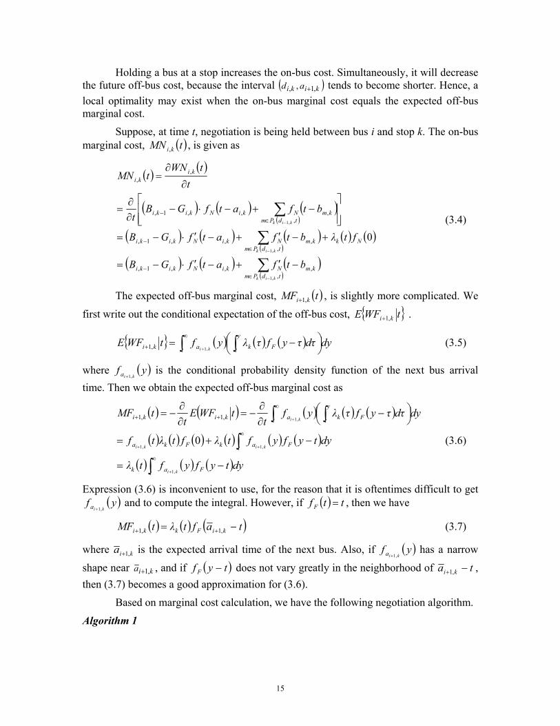
Holding a bus at a stop increases the on-bus cost. Simultaneously, it will decrease the future off-bus cost, because the interval ( )kiki ad ,1, , + tends to become shorter. Hence, a local optimality may exist when the on-bus marginal cost equals the expected off-bus marginal cost.

Suppose, at time t, negotiation is being held between bus i and stop k. The on-bus marginal cost, , is given as ( )tMN ki,

( ) ( )

( ) ( ) ( )( )

( ) ( ) ( )( )

( ) ( )

( ) ( ) ( )( )∑

∑

∑

−

−

−

∈−

∈−

∈−

−′+−′⋅−=

+−′+−′⋅−=

−+−⋅−

∂∂

=

∂

∂=

tdPmkmNkiNkiki

NktdPm

kmNkiNkiki

tdPmkmNkiNkiki

kiki

kik

kik

kik

btfatfGB

ftλbtfatfGB

btfatfGBt

ttWN

tMN

,,,,1,

,,,,1,

,,,,1,

,,

,1

,1

,1

0 (3.4)

The expected off-bus marginal cost, ( )tki ,1+MF , is slightly more complicated. We

first write out the conditional expectation of the off-bus cost, { }tWFE ki ,1+ .

{ } ( ) ( ) ( )∫ ∫∞

+

−=

+t

y

t Fkaki dyτdτyfτλyftWFEki ,1,1 (3.5)

where is the conditional probability density function of the next bus arrival time. Then we obtain the expected off-bus marginal cost as

( )yfkia ,1+

( ) ( ) ( ) ( ) ( )

( ) ( ) ( ) ( ) ( ) ( )

( ) ( ) ( )∫∫

∫ ∫

∞

∞

∞

++

−=

−+=

−

∂∂

−=∂∂

−=

+

++

+

t Fak

t FakFka

t

y

t Fkakiki

dytyfyftλ

dytyfyftλftλtf

dyτdτyfτλyft

tWFEt

tMF

ki

kiki

ki

,1

,1,1

,1

0

,1,1

(3.6)

Expression (3.6) is inconvenient to use, for the reason that it is oftentimes difficult to get and to compute the integral. However, if ( )yf

kia ,1+( ) ttf F = , then we have

( ) ( ) ( )taftλtMF kiFkki −= ++ ,1,1 (3.7)

where kia ,1+ is the expected arrival time of the next bus. Also, if has a narrow

shape near

( )yfkia ,1+

kia ,1+ , and if does not vary greatly in the neighborhood of ( tyf F − ) tkia −+ ,1 , then (3.7) becomes a good approximation for (3.6).

Based on marginal cost calculation, we have the following negotiation algorithm.

Algorithm 1

15

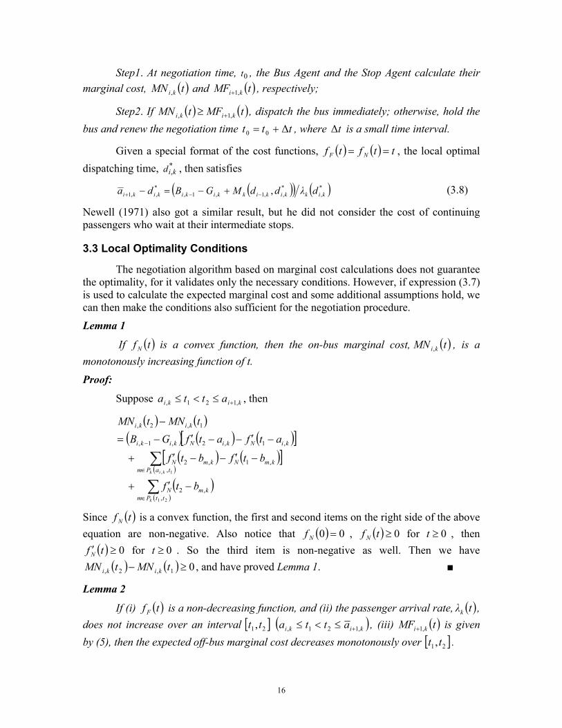
Step1. At negotiation time, t , the Bus Agent and the Stop Agent calculate their marginal cost, and

0

( )tMN ki , ( )MFi 1+ tk, , respectively;

Step2. If ( ) ( )tMFtMN kiki ,1, +≥

0

, dispatch the bus immediately; otherwise, hold the bus and renew the negotiation time t tt ∆0 += , where ∆ is a small time interval. t

Given a special format of the cost functions, ( ) ( ) ttftf NF == , the local optimal dispatching time, , then satisfies *

,kid

( )( ) ( )*,

*,,1,1,

*,,1 , kikkikikkikikiki dλddMGBda −−+ +−=− (3.8)

Newell (1971) also got a similar result, but he did not consider the cost of continuing passengers who wait at their intermediate stops.

3.3 Local Optimality Conditions

The negotiation algorithm based on marginal cost calculations does not guarantee the optimality, for it validates only the necessary conditions. However, if expression (3.7) is used to calculate the expected marginal cost and some additional assumptions hold, we can then make the conditions also sufficient for the negotiation procedure.

Lemma 1

If is a convex function, then the on-bus marginal cost, , is a monotonously increasing function of t.

( )tf N ( )tMN ki,

Proof:

Suppose , then kiki atta ,121, +≤<≤

( ) ( )( ) ( ) ([ ]

( ) ( )[ ]( )

( )( )∑

∑

∈

∈

−

−′+

−′−−′+

−′−−′−=

−

21

1,

,,2

,,1,2

,1,2,1,

1,2,

ttPmkmN

taPmkmNkmN

kiNkiNkiki

kiki

k

kik

btf

btfbtf

atfatfGBtMNtMN

)

Since is a convex function, the first and second items on the right side of the above equation are non-negative. Also notice that

( )tf N

( ) 00 =Nf , ( ) 0≥tf N for , then for . So the third item is non-negative as well. Then we have

, and have proved Lemma 1. ■

0≥t( )′ tf N

,MN ki

0≥( )2 −t

0≥t( 1, tki ) 0≥MN

Lemma 2

If (i) is a non-decreasing function, and (ii) the passenger arrival rate,( )tf F ( )tλk , does not increase over an interval [ ]21,tt ( )kiki atta ,121, +≤<≤ , (iii) MF is given by (5), then the expected off-bus marginal cost decreases monotonously over [ ] .

( )tki ,1+

1,tt 2

16

Proof for Lemma 2 is apparent.

We know that holding a bus reduces the off-bus costs but can increase the on-bus costs. If we see the decrement of the off-bus cost as an offer and the increment of the on-bus cost as a price, then our effort is to maximize the net profit. Lemma 1 and Lemma 2 provide us with a direct solution. Lemma 1 says that the price is convex, and Lemma 2 says that the offer is concave (see Figure 3.3). Hence, the optimality arises when the slopes of the offer and the price are equal.

di k*

Price

Offer

ai+1ai k

FIGURE 3.3 OPTIMALITY CONDITION FOR NEGOTIATION BASED ON MARGINAL COST

Theorem 1

If (i) is a convex function, (ii)( )tf N ( )tf F is a non-decreasing function, (iii) the passenger arrival rate, , does not increase over an interval ( )tλk [ ]21,tt ( )kki tta 1, <≤ ia ,12 +≤ , and (iv) ( )tki ,1+MF is given by (3.7), then the optimal dispatching

time, , in [ , occurs when the marginal costs are equal, i.e. *,kid ]21,tt

( ) ( )*,,1

*,, kikikiki dMFdMN += .

Most of the conditions for Theorem 1 are reasonable. However, we assume the passenger arrival rate to be non-increasing over the negotiation period. This condition will hold for a stationary process, but for a non-stationary process, it may not. However, in real world situations, the passenger arrival rate most often has only one peak, occurring just before the scheduled bus arrival time. The optimal dispatching time is most likely to be after that peak and before the next peak. Thus, the negotiation algorithm based on marginal cost calculations is still relevant.

3.4 Hyperopic Considerations

Although we have got an efficient algorithm for negotiation between a Stop Agent and a Bus Agent, we still have no guarantee of global optimality yet. This is because optimality of each single stop does not imply optimality of the entire line. Here is a simple example. When a bus is being held at a stop, hoping that its profit will increase, many passengers, who wait for it at downstream stops, will get impatient. The system has to be penalized for the “myopia” of this bus.

A wider range of negotiation may be needed to overcome this “myopia”. A Bus Agent may not only negotiate with the exact stop, at which it stands, but it may also need to negotiate with several downstream stops, where passengers are waiting. A further

17

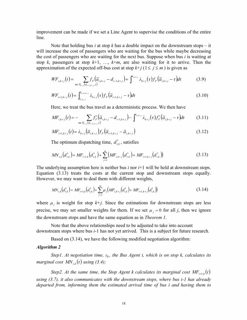
improvement can be made if we set a Line Agent to supervise the conditions of the entire line.

Note that holding bus i at stop k has a double impact on the downstream stops – it will increase the cost of passengers who are waiting for the bus while maybe decreasing the cost of passengers who are waiting for the next bus. Suppose when bus i is waiting at stop k, passengers at stop k+1, …, k+m, are also waiting for it to arrive. Then the approximation of the expected off-bus cost at stop k+j ( mj ≤≤1 ) is given as

( ) ( )( )

( ) ( )∫∑ +

+−+

−+−= ++∈

+−++jki

jkijk

a

t jkiFjktdPm

jkijkiFjki τdτafτλdaftWF ,

,1

,,

,1,, (3.9)

( ) ( ) ( )∫++

+

−= +++++jki

jki

a

a jkiFjkjki τdτafτλtWF ,1

,,1,1 (3.10)

Here, we treat the bus travel as a deterministic process. We then have

( ) ( )( )

( ) ( )∫∑ +

+−+

−′−−′−= ++∈

+−++jki

jkijk

a

t jkiFjktdPm

jkijkiFjki τdτafτλdaftMF ,

,1

,,

,1,, (3.11)

( ) ( ) ( )jkijkiFjkijkjki aafaλtMF +++++++ −= ,,1,,1 (3.12)

The optimum dispatching time, , satisfies *,kid

( ) ( ) ( ) ((∑=

++++ ++=m

jkijkikijkikikikiki dMFdMFdMFdMN

1

*,,1

*,,

*,,1

*,, )

)

) (3.13)

The underlying assumption here is neither bus i nor i+1 will be held at downstream stops. Equation (3.13) treats the costs at the current stop and downstream stops equally. However, we may want to deal them with different weights,

( ) ( ) ( ) ((∑=

++++ ++=m

jkijkikijkijkikikiki dMFdMFdMFdMN

1

*,,1

*,,

*,,1

*,, µ ) (3.14)

where jµ is weight for stop k+j. Since the estimations for downstream stops are less precise, we may set smaller weights for them. If we set 0=jµ for all j, then we ignore the downstream stops and have the same equation as in Theorem 1.

Note that the above relationships need to be adjusted to take into account downstream stops where bus i-1 has not yet arrived. This is a subject for future research.

Based on (3.14), we have the following modified negotiation algorithm:

Algorithm 2

Step1. At negotiation time, t , the Bus Agent i, which is on stop k, calculates its marginal cost using (3.4);

0

( )tMN ki ,

Step2. At the same time, the Stop Agent k calculates its marginal cost ( )tki ,1+MF using (3.7), it also communicates with the downstream stops, where bus i-1 has already departed from, informing them the estimated arrival time of bus i and having them to

18

calculate their marginal costs, ( )tjki +,MF , ( )tMF jki ++ ,1

( )( + +jki tMF ,

(j=1,2,…, m, where m is the number of involved downstream stops), based on their local data and using (3.11) and (3.12);

( ) ∑=

+ +m

jk t

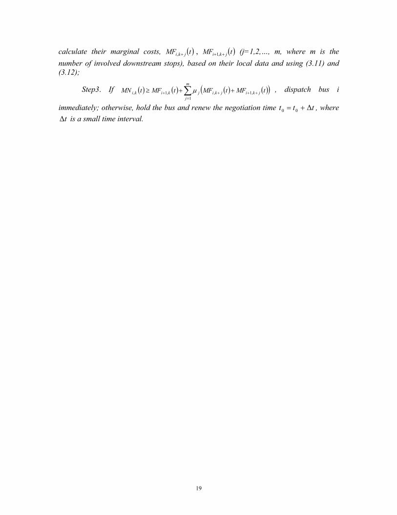
1,1 µStep3. If , dispatch bus i

immediately; otherwise, hold the bus and renew the negotiation time t , where is a small time interval.

( ) ( )++≥ jkijiki tMFMFtMN ,1,

tt ∆00 +=t∆

)

19

4. Simulation – Stationary Passenger Arrivals

4.1 Basic Settings

4.1.1 Physical Parameters

We set up a line with NS stops and NB buses. Passenger arrivals at each stop are a stationary Poisson process and have the same arrival rate, λ . Also, the passenger alighting ratio at each stop is given by ρ . The travel time between two stops is a log-normal random variable with a mean of TBS and a variance of . Cost functions are

. We also consider the dwelling (boarding only) time for each passenger, DW, which is a constant. If no special specification, the basic parameters of the route in our simulations are: NS ,

2σ( ) ( ) ttftf NF ==

10= min5=TBS , , 42 =σ min/0.1=λ , 4.0=ρ , . In all scenarios, we make 10 simulation runs with each run being 1200 minutes.

min05.0=DW

4.1.2 Set of Strategies

We test and compare the following four strategies:

1. No-Wait strategy: Buses are not held at stops, and they leave immediately after passenger unloading and loading.

2. Even-Headway strategy: A bus is held at a stop (beyond unloading and loading) in order to make the headway between the current and the preceding bus equal to that between the current and the succeeding bus.

3. On-Schedule strategy: A bus is held at a stop (beyond unloading and loading) only if it arrives earlier than the scheduled arrival time. Note that in most transit systems the scheduled arrival time is typically longer than the expected actual arrival time since there is typically some slack in the schedule (Dessouky, et al., 1999). That is, if TBS is the expected travel time between two stops, then the scheduled travel time is

, where s is the slackness. ( sTBS +⋅ 1 )

4. Negotiation strategy using marginal costs: Buses are held (beyond unloading and loading) according to Algorithm 2, 1=jµ for all j.

4.2 Simulation Results

4.2.1 Scenario 1 – Straight Line with Different Scheduled Headways

In this scenario, we assume there is sufficient slack only at the terminal stop in the schedule so that all buses leave on time at the terminal stop. This scenario is equivalent to viewing the route as a straight line instead of as a loop.

We assume the slackness, s, for these experiments to be .3. This is comparable to the amount of slack found on bus lines in LAC/MTA (Dessouky et al., 1999). We simulate the route with different headways. Figure 4.1 shows the savings (comparing with the No-Wait strategy) under different headways. As the figure shows, the Negotiation strategy outperforms the other strategies especially when the headway is less

20

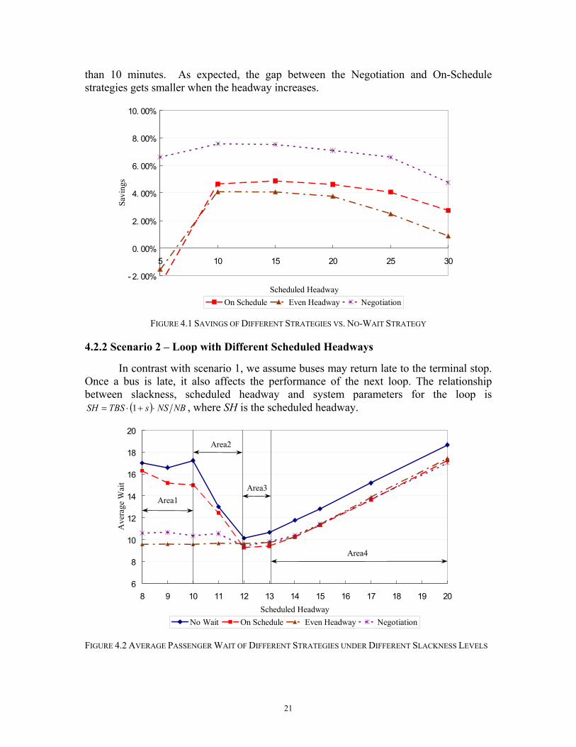
than 10 minutes. As expected, the gap between the Negotiation and On-Schedule strategies gets smaller when the headway increases.

- 2. 00%

0. 00%

2. 00%

4. 00%

6. 00%

8. 00%

10. 00%

5 10 15 20 25 3

Scheduled Headway

Savi

ngs

On Schedule Even Headway Negotiation

0

FIGURE 4.1 SAVINGS OF DIFFERENT STRATEGIES VS. NO-WAIT STRATEGY

4.2.2 Scenario 2 – Loop with Different Scheduled Headways

In contrast with scenario 1, we assume buses may return late to the terminal stop. Once a bus is late, it also affects the performance of the next loop. The relationship between slackness, scheduled headway and system parameters for the loop is

( ) NBNSsTBSSH ⋅+⋅= 1 , where SH is the scheduled headway.

6

8

10

12

14

16

18

20

8 9 10 11 12 13 14 15 16 17 18 19 20Scheduled Headway

Ave

rage

Wai

t

No Wait On Schedule Even Headway Negotiation

Area1

Area2

Area3

Area4

FIGURE 4.2 AVERAGE PASSENGER WAIT OF DIFFERENT STRATEGIES UNDER DIFFERENT SLACKNESS LEVELS

21

We first try to determine the best level of s for the different strategies. Figure 4.2 shows that area 3 is the best working area for all strategies, i.e. slackness, s, should be between 0.2 and 0.3. This result is consistent with the observation of Dessouky et al. (1999) on Los Angeles County routes, which have slackness of 0.25.

In Area 1 (a system suffering sudden bus breakdowns may lie in this area), the No-Wait and On-Schedule strategies are unstable since the buses cannot make the schedule under these slackness levels. However, the Even-Headway and Negotiation strategies are stable in this region. That is, under these strategies, the average wait times reach near steady state values. This is because Even-Headway and Negotiation strategies are schedule-independent strategies and have relatively strong self-adjustment ability. In this case, the actual headway is larger than the scheduled headway but the coefficient of variation of actual headway, C , are almost constant and small (we will later show this result). In Area 2, the average wait times for the No-Wait and On-Schedule strategies decrease significantly as the slackness increases. In Area 3, all strategies are stable and this area contains the best level of slackness in the schedule. Area 4 shows that as the slackness continues to increase the average wait will then increase. In summary, scheduled headway of 12 minimizes the average wait for this scenario, and at this slackness, all the strategies except No-Wait perform equally well.

( )2H

Note that Osuna and Newell (1972) show that in the stationary case the average wait is a function of C . We next show ( )2H ( )2HC at each stop. We use a slackness of 0.2 (i.e. a scheduled headway of 12) for this analysis. The results are shown in Figure 4.3. Note that although the Even-Headway strategy has the minimum ( )2HC , it also has the largest average headway of 13.6, while the others have an average headway of 12 (see Figure 4.4).

0

0.1

0.2

0.3

0.4

0.5

0.6

0.7

0.8

1 2 3 4 5 6 7 8 9 1

STOP INDEX

C(H

)^2

No Wait On Schedule Even Headway Negotiation

0

FIGURE 4.3 COEFFICIENT OF VARIATION OF HEADWAYS OF DIFFERENT STRAEGIES AT EACH STOP

22

11.5

12

12.5

13

13.5

14

1 2 3 4 5 6 7 8 9 1

STOP INDEX

AV

ERA

GE

HEA

DW

AY

No Wait On Schedule Even Headway WRN

0

FIGURE 4.4 AVERAGE HEADWAYS OF DIFFERENT STATEGIES AT EACH STOP

23

5. Simulation – Non-Stationary Passenger Arrivals

5.1 Passenger Arrivals in Bursts

5.1.1 Physical Parameters

We assume that there is sufficient slack at the terminal stop so that the buses can always depart on time at the terminal stop. In this case, the route of the transit network can be considered as a straight line. The physical parameters for the route are: 10=NS ,

, , min5=TBS 42 =σ 4.0=ρ , min05.0=DW . These parameters are the same as in Section 4.3.1 except for the passenger arrival rates.

0

2

4

6

8

10

12

14

16

18

500 520 540 560 580 600

Time

Arr

ival

Rat

e

FIGURE 5.1 PASSENGER ARRIVAL RATE WITH RANDOM BURSTS

In this part, the passenger arrival rate is not constant (see Figure 5.1) but consists of random peaks representing bursts of passenger arrivals. This situation may happen when the passenger arrivals are related to specific random events. Some examples of this passenger arrival pattern include audiences coming out in random bursts after short events or shows in amusement parks such as Disneyland, movie complexes, and downtown corridors, as well as passenger arrivals at transfer stops of a transit network. In these cases, a large number of passengers arrive when the random event happens (the show ends or the bus carrying transferring passengers arrives). We assume that each peak is a gaussian function of time (or we could say, during a certain period, passenger arrival times are normally distributed), and the length of each peak period is exponentially distributed with mean of α . However, the average arrival rate λ for each period is a constant. Hence, the arrival rate during each period can be expressed as

24

( )

( )

( )

+<≤−

−−

−−⋅

=

∫+

−

22 ,

2exp

2exp

2

2

2

2

2

2

LttLt

dt

ttLλ

t ppt

t p

p

p

p

Lp

Lp

τσ

τ

σλ (5.1)

where is the length of the period, t is the midpoint of the period (i.e., peak time), and

is the variance of the normal distribution.

L p

2pσ

5.1.2 Set of Strategies

In this part, for Negotiation strategy, we set 0=jµ for all j. The reason is that the passenger arrivals at downstream stops are non-stationary with random bursts, i.e., they resemble a white noise sequence. Therefore the estimates of future passenger arrivals become unreliable. Hence, prediction of marginal costs at downstream stops does not help much, and may even worsen the solution quality, in this situation.

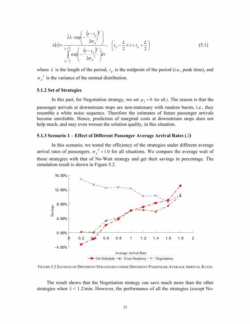
5.1.3 Scenario 1 – Effect of Different Passenger Average Arrival Rates (λ)

In this scenario, we tested the efficiency of the strategies under different average arrival rates of passengers. for all situations. We compare the average wait of those strategies with that of No-Wait strategy and get their savings in percentage. The simulation result is shown in Figure 5.2.

0.12 =pσ

- 4. 00%

0. 00%

4. 00%

8. 00%

12. 00%

16. 00%

0 0. 2 0. 4 0. 6 0. 8 1 1. 2 1. 4 1. 6 1. 8 2

Average Arrival Rate

Savi

ngs

On Schedule Even Headway Negotiation

FIGURE 5.2 SAVINGS OF DIFFERENT STRATEGIES UNDER DIFFERENT PASSENGER AVERAGE ARRIVAL RATES

The result shows that the Negotiation strategy can save much more than the other strategies when λ < 1.2/min. However, the performance of all the strategies (except No-

25

Wait strategy) are close to each other for λ >1.2. Overall, the savings of the Negotiation strategy are greater in this non-stationary case than for the previous stationary scenario.

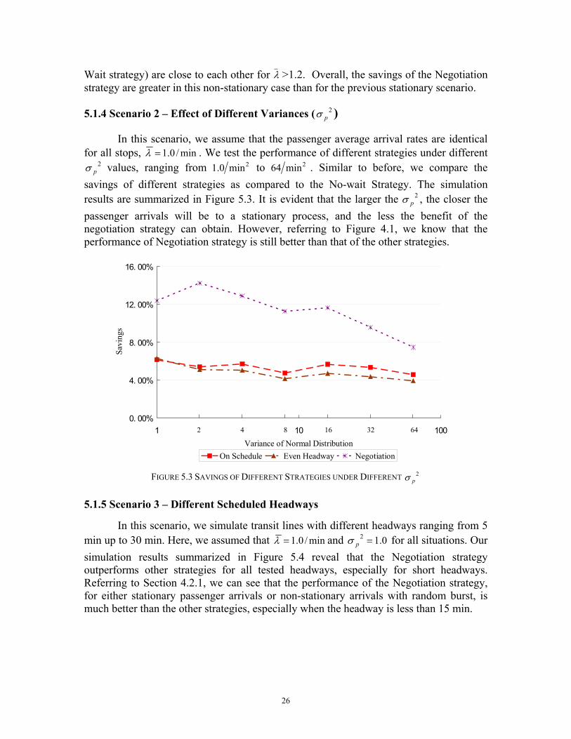
5.1.4 Scenario 2 – Effect of Different Variances ( ) 2pσ

In this scenario, we assume that the passenger average arrival rates are identical for all stops, min/0.1=λ . We test the performance of different strategies under different

values, ranging from 2pσ 2min0.1 to 2min64 . Similar to before, we compare the

savings of different strategies as compared to the No-wait Strategy. The simulation results are summarized in Figure 5.3. It is evident that the larger the , the closer the passenger arrivals will be to a stationary process, and the less the benefit of the negotiation strategy can obtain. However, referring to Figure 4.1, we know that the performance of Negotiation strategy is still better than that of the other strategies.

2pσ

0. 00%

4. 00%

8. 00%

12. 00%

16. 00%

1 10 100Variance of Normal Distribution

Savi

ngs

On Schedule Even Headway Negotiation

2 4 8 16 32 64

FIGURE 5.3 SAVINGS OF DIFFERENT STRATEGIES UNDER DIFFERENT 2

pσ

5.1.5 Scenario 3 – Different Scheduled Headways

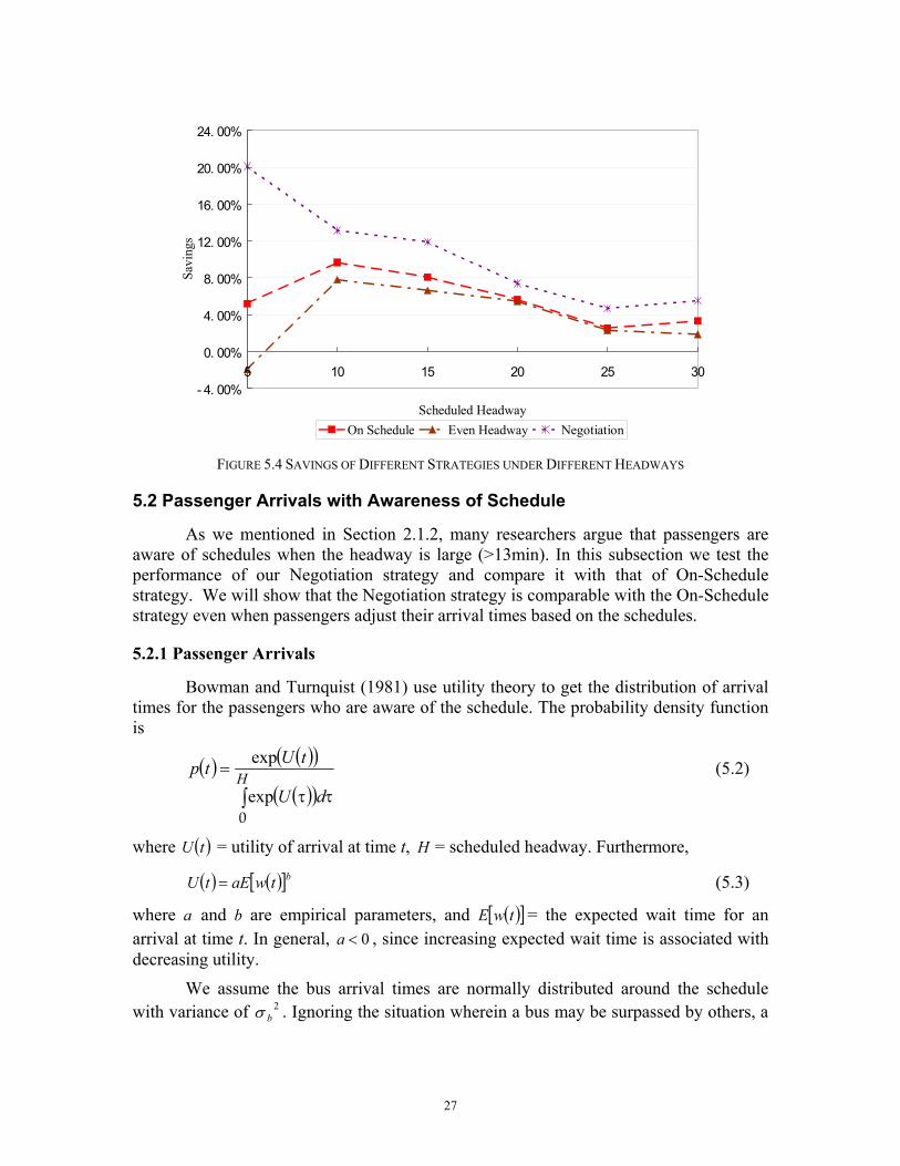
In this scenario, we simulate transit lines with different headways ranging from 5 min up to 30 min. Here, we assumed that min/0.1=λ and for all situations. Our simulation results summarized in Figure 5.4 reveal that the Negotiation strategy outperforms other strategies for all tested headways, especially for short headways. Referring to Section 4.2.1, we can see that the performance of the Negotiation strategy, for either stationary passenger arrivals or non-stationary arrivals with random burst, is much better than the other strategies, especially when the headway is less than 15 min.

0.12 =pσ

26

- 4. 00%

0. 00%

4. 00%

8. 00%

12. 00%

16. 00%

20. 00%

24. 00%

5 10 15 20 25 3

Scheduled Headway

Savi

ngs

On Schedule Even Headway Negotiation

0

FIGURE 5.4 SAVINGS OF DIFFERENT STRATEGIES UNDER DIFFERENT HEADWAYS

5.2 Passenger Arrivals with Awareness of Schedule

As we mentioned in Section 2.1.2, many researchers argue that passengers are aware of schedules when the headway is large (>13min). In this subsection we test the performance of our Negotiation strategy and compare it with that of On-Schedule strategy. We will show that the Negotiation strategy is comparable with the On-Schedule strategy even when passengers adjust their arrival times based on the schedules.

5.2.1 Passenger Arrivals

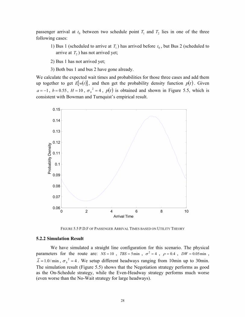
Bowman and Turnquist (1981) use utility theory to get the distribution of arrival times for the passengers who are aware of the schedule. The probability density function is

( ) ( )( )

( )( )∫ ττ

= HdU

tUtp

0exp

exp (5.2)

where U = utility of arrival at time t, ( )t H = scheduled headway. Furthermore,

(5.3) ( ) ( )[ ]btwaEtU =

where and are empirical parameters, and a b ( )[ ]twE = the expected wait time for an arrival at time t. In general, a , since increasing expected wait time is associated with decreasing utility.

0<

We assume the bus arrival times are normally distributed around the schedule with variance of . Ignoring the situation wherein a bus may be surpassed by others, a 2

bσ

27

passenger arrival at t between two schedule point T and lies in one of the three following cases:

0

2

w10=

1 2T

0t

4

1) Bus 1 (scheduled to arrive at T ) has arrived before , but Bus 2 (scheduled to arrive at T ) has not arrived yet;

1

2) Bus 1 has not arrived yet;

3) Both bus 1 and bus 2 have gone already.

We calculate the expected wait times and probabilities for those three cases and add them up together to get E , and then get the probability density function p . Given

, , , , ( )[ tσ

] ( )t1−=a 55.0=b H 42 =b ( )tp is obtained and shown in Figure 5.5, which is

consistent with Bowman and Turnquist’s empirical result.

0 2 4 6 8 100.06

0.07

0.08

0.09

0.1

0.11

0.12

0.13

0.14

0.15

Arrival Time

Pro

babl

ity D

ensi

ty

FIGURE 5.5 P.D.F OF PASSENGER ARRIVAL TIMES BASED ON UTILITY THEORY

5.2.2 Simulation Result

We have simulated a straight line configuration for this scenario. The physical parameters for the route are: 10=NS , min5=TBS , , 2 =σ 4.0=ρ , , min05.0=DW

min/0.1=λ , . We setup different headways ranging from 10min up to 30min. The simulation result (Figure 5.5) shows that the Negotiation strategy performs as good as the On-Schedule strategy, while the Even-Headway strategy performs much worse (even worse than the No-Wait strategy for large headways).

42 =bσ

28

- 10. 00%

- 5. 00%

0. 00%

5. 00%

10. 00%

15. 00%

20. 00%

10 15 20 25 30

Scheduled Headway

Savi

ngs

On Schedule Even Headway Negotiation

FIGURE 5.6 PERFORMANCE COMPARING OF DIFFERENT STRATEGIES WITH AWARE PASSENGERS

29

6. Conclusion The bus-holding problem has been studied for many years. Various strategies

have been presented to address this problem. The most common and the simplest method is the On-Schedule strategy. It utilizes only the stationary statistics but not the real-time information. The Even-Headway strategy uses only the real-time information regarding the departure time of the last bus. In recent years, many studies focus on developing real-time control strategies, intending to obtain better coordination of the system. However, none of the available methods is adequately robust for application in a wide range of transit scenarios. The main objective of our project has been to develop a robust method for the coordination of transit operations, applicable to a wide range of transit environments.

We have developed a negotiation-based framework, wherein stops and buses act as agents. They negotiate based on their marginal costs. Our work proves that under some reasonable assumptions, the framework can find locally optimal dispatching times. Our distributed holding control approach distinguishes itself for its ability to harness real-time information and to make decisions directly based on the marginal wait cost. To verify the efficiency of our strategy, we also developed a simulation system. We performed simulations for stationary as well as different kinds of non-stationary passenger arrivals. The simulation results verify that our framework is robust and adequate for coordination in a wide range of transit environments.

Another advantage of our negotiation algorithm is that it can consider the wait of continuing passengers with different types of cost functions. In other words, the negotiation algorithm is more flexible and generic compared to the existing transit control methods. Our simulations also show that simple strategies, i.e. On-schedule and Even-headway strategies, are adequate for a narrow range of transit situations where passenger arrivals are stationary. However, for non-stationary situations such as those present in amusement parks, airports, schools, etc., these simple strategies are not adequate and our negotiation-based framework provides significantly better solutions.

30

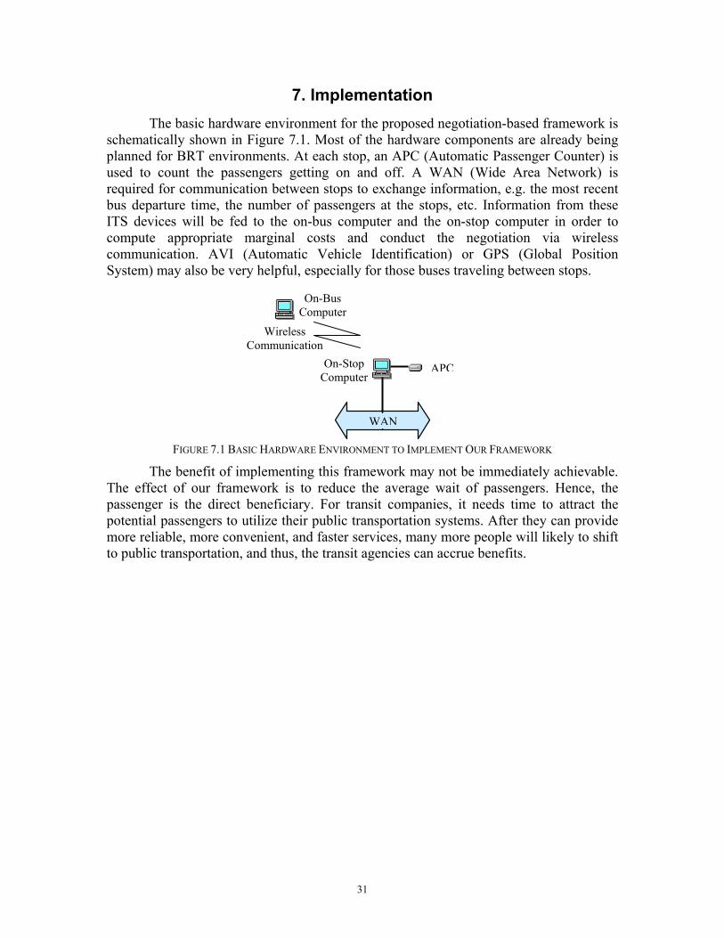
7. Implementation The basic hardware environment for the proposed negotiation-based framework is

schematically shown in Figure 7.1. Most of the hardware components are already being planned for BRT environments. At each stop, an APC (Automatic Passenger Counter) is used to count the passengers getting on and off. A WAN (Wide Area Network) is required for communication between stops to exchange information, e.g. the most recent bus departure time, the number of passengers at the stops, etc. Information from these ITS devices will be fed to the on-bus computer and the on-stop computer in order to compute appropriate marginal costs and conduct the negotiation via wireless communication. AVI (Automatic Vehicle Identification) or GPS (Global Position System) may also be very helpful, especially for those buses traveling between stops.

WAN

APC

Wireless Communication

On-Stop Computer

On-Bus Computer

FIGURE 7.1 BASIC HARDWARE ENVIRONMENT TO IMPLEMENT OUR FRAMEWORK

The benefit of implementing this framework may not be immediately achievable. The effect of our framework is to reduce the average wait of passengers. Hence, the passenger is the direct beneficiary. For transit companies, it needs time to attract the potential passengers to utilize their public transportation systems. After they can provide more reliable, more convenient, and faster services, many more people will likely to shift to public transportation, and thus, the transit agencies can accrue benefits.

31

References [1] Andersson, P., Hermansson, A., Tengvald, E. and Scalia-Tomba, G. (1979),

“Analysis and Simulation of an Urban Bus Route,” Transportation Research, Vol.13A, 439-466

[2] Andersson, P. and Scalia-Tomba, G. (1981), “A Mathematical Model of an Urban Bus Route,” Transportation Science, Vol.15B, 249-266

[3] Barnett, A. (1974). “On Controlling Randomness in Transit Operations,” Transportation Science, Vol. 8, pp. 102-116.

[4] Barnett, A. (1978). “Control Strategies for Transport Systems with Nonlinear Waiting Costs,” Transportation Science, Vol. 12, pp. 119-136.

[5] Bazan, A. (1995). “A Game-Theoretic Approach to Distributed Control of Traffic Signals,” Proc. First International Conf. on Multi-Agent Systems, pp. 439.

[6] Bowman, L. A., and M. A. Turnquist (1981). “Service frequency, Schedule Reliability and Passenger Wait Times at Transit Stops,” Transportation Research, Vol. 15A, pp. 465-471.

[7] Burmeister, B., Haddadi, A. and Matylis, G. (1997), “Application of Multi-Agent Systems in Traffic and Transportation,” IEEE Tansactions on Software Engineering, Vol.144, 51-60.

[8] Dessouky, M., R. Hall, A. Nowroozi, and K. Mourikas (1999). “Bus Dispatching at Timed Transfer Transit Stations Using Bus Tracking Technology,” Transportation Research, Vol. 7C, pp. 187-208.

[9] Eberlein, X. J., N. H. M. Wilson, C. Barnhart, and D. Bernstein (1998). “The Real-Time Deadheading Problem in Transit Operations Control,” Transportation Research, Vol. 32B, pp. 77-100.

[10] Eberlein, X. J., N. H. M. Wilson, D. Bernstein (2001). “The Holding Problem with Real-Time Information Available,” Transportation Science, Vol. 35, No. 1, pp. 1-18.

[11] Jolliffe, J. K., and T. P. Hutchinson (1975). “A Behavioral Explanation of Association Between Bus and Passenger Arrivals at a Bus Stop,” Transportation Science, Vol. 9, pp. 248-292.

[12] Kohout, R. and K. Erol (1999). “In-Time Agent-Based Vehicle Routing with a Stochastic Improvement Heuristic,” Proc. Sixteenth National Conf. on Artificial Intelligence (AAI-99). Eleventh Innovative Applications of Artificial Intelligence Conf. (IAAI-99), pp. 864-869.

[13] Lin, G., Liang, P., Schonfeld, P. and Larson, R. (1995), “Adaptive Control of Transit Operations,” U.S. Department of Transportation, Report No. MD-26-7002.

[14] Manikonda, V., Levy, R., Satapathy, G., Lovell, D. J., Chang, P. C., and Teittinen, A. (2000). “Autonomous Agents for Traffic Simulation and Control,” Technique Report.

32

[15] Newell, G. F. (1971). “Dispatching Policies for a Transportation Route”, Transportation Science, Vol. 5, pp. 91-105.

[16] Newell, G. F. (1974). “Control of Pairing of Buses on a Public Transportation Route, Two Buses, One Control Point,” Transportation Science, Vol. 8, pp. 248-264.

[17] Okrent, M. M. (1974). “Effects of Transit Service Characteristics on Passenger Waiting Time,” M.S. Thesis, Northwestern University, Department of Civil Engineering, Evanston, Illinois.

[18] Osuna, E. E., and G. F. Newell (1972). “Control Strategies for an Idealized Public Transportation System,” Transportation Science, Vol. 6, pp. 52-72.

[19] Powell, W. B. and Sheffi, Y. (1983), “A Probabilistic Model of Bus Route Performance,” Transportation Science, Vol.17, 376-404.

[20] Powell, W. B. (1983). “Bulk Service Queues with Deviations from Departure Schedules: The Problem of Correlated Headways,” Transportation Research, Vol. 17B, pp. 221-232.

[21] Powell, W. B. (1985). “Analysis of Bus Holding and Cancellation Strategies in Bulk Arrival, Bulk Service Queues,” Transportation Science, Vol. 6, pp. 52-77.

[22] Sandholm, T. (1993). “An Implementation of the Contract Net Protocol Based On Marginal Cost Calculations,” Proc. of the Eleventh National Conference on Artificial Intelligence, pp. 256-262.

[23] Satapathy, G., and S. R. T. Kumara (2000). “Negotiation for Transportation Tasks with Stochastic Payoffs,” Computer in Industry, 42(2-3), pp. 193-202.

[24] Schiemek, P., “BRT Reference Guide,” DOT Archives, http://brt.uolpe.dot.gov/guide/

[25] Senevirante, P. N. (1990), “Analysis of On-Time Performance of Bus Services Using Simulation,” Journal of Transportation Engineering, Vol.116, 517-531

33

34

Appendix 1

Nomenclature used in this report:

ai,k – actual arrival time of bus i at stop k

di,k – actual departure time of bus i from stop k

Di,k – scheduled departure time of bus i from stop k

Rk – scheduled travel time from stop k-1 to stop k

Bi,k – number of passengers on bus i when departing from stop k

Gi,k – number of passengers alighting bus i at stop k

Mk(t1,t2) – number of passengers that have arrived at stop k over an interval (t1,t2)

Pk(t1,t2) – set of passengers that have arrived at stop k over an interval (t1,t2)

tm,k – arrival time of passenger m at stop k, m∈ Pk(t1,t2)

bm,k – boarding time of passenger m at stop k, m∈ Pk(t1,t2)