Distributed algorithms for connected domination in wireless networks
15
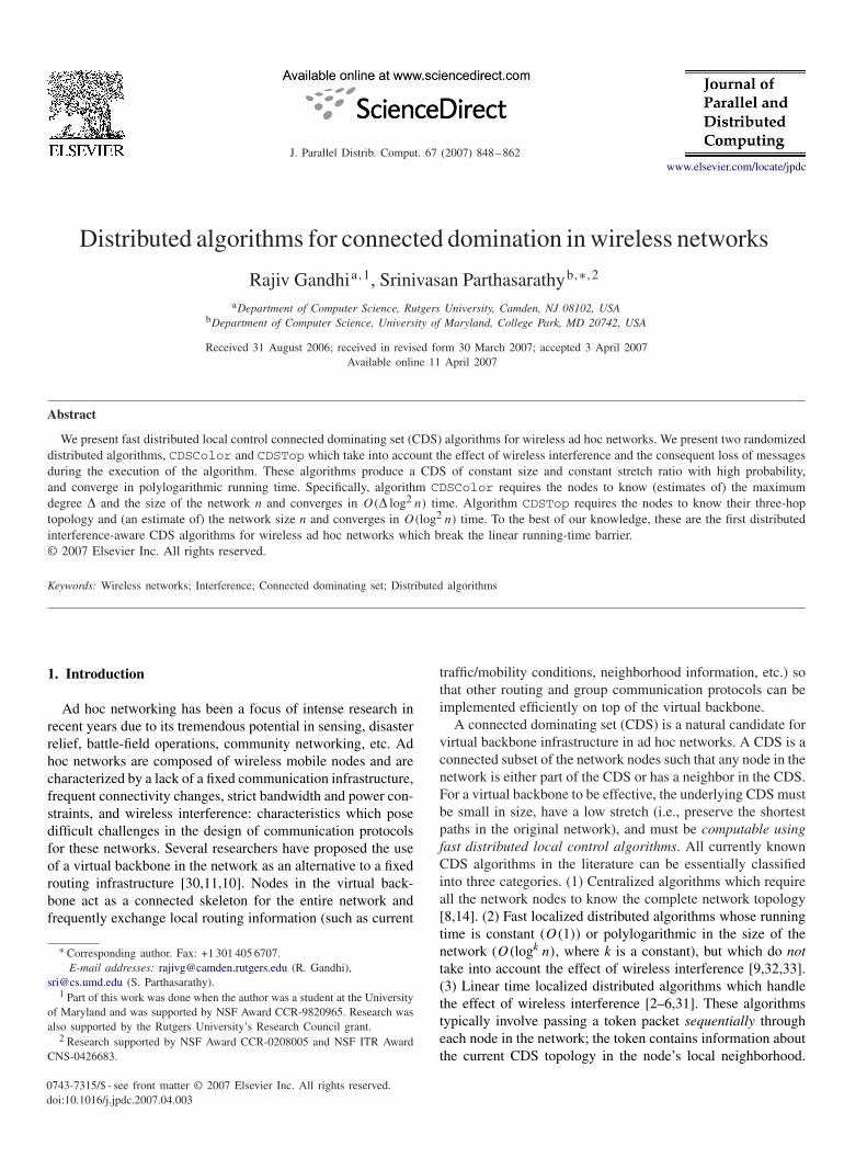
J. Parallel Distrib. Comput. 67 (2007) 848 – 862 www.elsevier.com/locate/jpdc Distributed algorithms for connected domination in wireless networks Rajiv Gandhi a , 1 , Srinivasan Parthasarathy b, ∗, 2 a Department of Computer Science, Rutgers University, Camden, NJ 08102, USA b Department of Computer Science, University of Maryland, College Park, MD 20742, USA Received 31 August 2006; received in revised form 30 March 2007; accepted 3 April 2007 Available online 11 April 2007 Abstract We present fast distributed local control connected dominating set (CDS) algorithms for wireless ad hoc networks. We present two randomized distributed algorithms, CDSColor and CDSTop which take into account the effect of wireless interference and the consequent loss of messages during the execution of the algorithm. These algorithms produce a CDS of constant size and constant stretch ratio with high probability, and converge in polylogarithmic running time. Specifically, algorithm CDSColor requires the nodes to know (estimates of) the maximum degree and the size of the network n and converges in O( log 2 n) time. Algorithm CDSTop requires the nodes to know their three-hop topology and (an estimate of) the network size n and converges in O(log 2 n) time. To the best of our knowledge, these are the first distributed interference-aware CDS algorithms for wireless ad hoc networks which break the linear running-time barrier. © 2007 Elsevier Inc. All rights reserved. Keywords: Wireless networks; Interference; Connected dominating set; Distributed algorithms 1. Introduction Ad hoc networking has been a focus of intense research in recent years due to its tremendous potential in sensing, disaster relief, battle-field operations, community networking, etc. Ad hoc networks are composed of wireless mobile nodes and are characterized by a lack of a fixed communication infrastructure, frequent connectivity changes, strict bandwidth and power con- straints, and wireless interference: characteristics which pose difficult challenges in the design of communication protocols for these networks. Several researchers have proposed the use of a virtual backbone in the network as an alternative to a fixed routing infrastructure [30,11,10]. Nodes in the virtual back- bone act as a connected skeleton for the entire network and frequently exchange local routing information (such as current ∗ Corresponding author. Fax: +1 301 405 6707. E-mail addresses: [email protected] (R. Gandhi), [email protected] (S. Parthasarathy). 1 Part of this work was done when the author was a student at the University of Maryland and was supported by NSF Award CCR-9820965. Research was also supported by the Rutgers University’s Research Council grant. 2 Research supported by NSF Award CCR-0208005 and NSF ITR Award CNS-0426683. 0743-7315/$ - see front matter © 2007 Elsevier Inc. All rights reserved. doi:10.1016/j.jpdc.2007.04.003 traffic/mobility conditions, neighborhood information, etc.) so that other routing and group communication protocols can be implemented efficiently on top of the virtual backbone. A connected dominating set (CDS) is a natural candidate for virtual backbone infrastructure in ad hoc networks. A CDS is a connected subset of the network nodes such that any node in the network is either part of the CDS or has a neighbor in the CDS. For a virtual backbone to be effective, the underlying CDS must be small in size, have a low stretch (i.e., preserve the shortest paths in the original network), and must be computable using fast distributed local control algorithms. All currently known CDS algorithms in the literature can be essentially classified into three categories. (1) Centralized algorithms which require all the network nodes to know the complete network topology [8,14]. (2) Fast localized distributed algorithms whose running time is constant (O(1)) or polylogarithmic in the size of the network (O(log k n), where k is a constant), but which do not take into account the effect of wireless interference [9,32,33]. (3) Linear time localized distributed algorithms which handle the effect of wireless interference [2–6,31]. These algorithms typically involve passing a token packet sequentially through each node in the network; the token contains information about the current CDS topology in the node’s local neighborhood.
-
Upload
rajiv-gandhi -
Category
Documents
-
view
213 -
download
0
Transcript of Distributed algorithms for connected domination in wireless networks
J. Parallel Distrib. Comput. 67 (2007) 848–862www.elsevier.com/locate/jpdc
Distributed algorithms for connected domination in wireless networks
Rajiv Gandhia,1, Srinivasan Parthasarathyb,∗,2
aDepartment of Computer Science, Rutgers University, Camden, NJ 08102, USAbDepartment of Computer Science, University of Maryland, College Park, MD 20742, USA
Received 31 August 2006; received in revised form 30 March 2007; accepted 3 April 2007Available online 11 April 2007
Abstract
We present fast distributed local control connected dominating set (CDS) algorithms for wireless ad hoc networks. We present two randomizeddistributed algorithms, CDSColor and CDSTop which take into account the effect of wireless interference and the consequent loss of messagesduring the execution of the algorithm. These algorithms produce a CDS of constant size and constant stretch ratio with high probability,and converge in polylogarithmic running time. Specifically, algorithm CDSColor requires the nodes to know (estimates of) the maximumdegree � and the size of the network n and converges in O(� log2 n) time. Algorithm CDSTop requires the nodes to know their three-hoptopology and (an estimate of) the network size n and converges in O(log2 n) time. To the best of our knowledge, these are the first distributedinterference-aware CDS algorithms for wireless ad hoc networks which break the linear running-time barrier.© 2007 Elsevier Inc. All rights reserved.
Keywords: Wireless networks; Interference; Connected dominating set; Distributed algorithms
1. Introduction
Ad hoc networking has been a focus of intense research inrecent years due to its tremendous potential in sensing, disasterrelief, battle-field operations, community networking, etc. Adhoc networks are composed of wireless mobile nodes and arecharacterized by a lack of a fixed communication infrastructure,frequent connectivity changes, strict bandwidth and power con-straints, and wireless interference: characteristics which posedifficult challenges in the design of communication protocolsfor these networks. Several researchers have proposed the useof a virtual backbone in the network as an alternative to a fixedrouting infrastructure [30,11,10]. Nodes in the virtual back-bone act as a connected skeleton for the entire network andfrequently exchange local routing information (such as current
∗ Corresponding author. Fax: +1 301 405 6707.E-mail addresses: [email protected] (R. Gandhi),
[email protected] (S. Parthasarathy).1 Part of this work was done when the author was a student at the University
of Maryland and was supported by NSF Award CCR-9820965. Research wasalso supported by the Rutgers University’s Research Council grant.
2 Research supported by NSF Award CCR-0208005 and NSF ITR AwardCNS-0426683.
0743-7315/$ - see front matter © 2007 Elsevier Inc. All rights reserved.doi:10.1016/j.jpdc.2007.04.003
traffic/mobility conditions, neighborhood information, etc.) sothat other routing and group communication protocols can beimplemented efficiently on top of the virtual backbone.
A connected dominating set (CDS) is a natural candidate forvirtual backbone infrastructure in ad hoc networks. A CDS is aconnected subset of the network nodes such that any node in thenetwork is either part of the CDS or has a neighbor in the CDS.For a virtual backbone to be effective, the underlying CDS mustbe small in size, have a low stretch (i.e., preserve the shortestpaths in the original network), and must be computable usingfast distributed local control algorithms. All currently knownCDS algorithms in the literature can be essentially classifiedinto three categories. (1) Centralized algorithms which requireall the network nodes to know the complete network topology[8,14]. (2) Fast localized distributed algorithms whose runningtime is constant (O(1)) or polylogarithmic in the size of thenetwork (O(logk n), where k is a constant), but which do nottake into account the effect of wireless interference [9,32,33].(3) Linear time localized distributed algorithms which handlethe effect of wireless interference [2–6,31]. These algorithmstypically involve passing a token packet sequentially througheach node in the network; the token contains information aboutthe current CDS topology in the node’s local neighborhood.

R. Gandhi, S. Parthasarathy / J. Parallel Distrib. Comput. 67 (2007) 848–862 849
Since the token is handled sequentially, there are no concurrenttransmissions and no packet losses due to interference; howeverthis imposes a linear running time on the algorithm.
Centralized CDS algorithms (from the first category) are hardto implement over an ad hoc network due to the difficulties in-volved in collecting and maintaining the entire network topol-ogy information at each node. Distributed algorithms whichdo not directly incorporate the effects of wireless interferencealso present difficult and open implementation challenges. Inparticular, it is unclear and a open a question if and how theunderlying message transmissions in these algorithms could bescheduled such that the algorithm converges quickly (in con-stant or polylog time), in the presence of message losses due tointerference. Linear-time distributed algorithms do not exploitthe massive parallelism available in the ad hoc network. Fur-ther, linear-time algorithms are more susceptible to disruptionscaused by network dynamics, since there is a high likelihoodof changes in network connectivity before the termination ofthe distributed algorithm.
The above discussion naturally leads us to the followingquestion: does there exist fast local control distributed algo-rithms for CDS construction in wireless ad hoc networks? Inthis work, we design two distributed CDS algorithms for wire-less ad hoc networks, which answer this question in the affirma-tive. Specifically, the following are the main results presentedin this paper.
1.1. Our contributions
We present provably good fast interference-aware distributedalgorithms for CDS construction in ad hoc networks. Whileseveral sublinear distributed CDS algorithms exist in the liter-ature, none of them explicitly incorporate the loss of messagesdue to wireless interference; our algorithms are guaranteed toconverge in polylogarithmic time and produce a valid CDS upontermination with high probability. To the best of our knowledge,ours is the first work to present rigorous, fast converging, localcontrol algorithmic techniques for CDS construction in wire-less ad hoc networks which take into account message lossesdue to interference, albeit with the assumption of synchronousnetwork communication.
We present two distributed algorithms: a Distance-2 color-ing based algorithm CDSColor and a neighborhood topologybased algorithm CDSTop. Algorithm CDSColor requires eachnode to know the maximum degree � and the total numberof network nodes n and runs in time O(� log2 n). AlgorithmCDSTop requires each node to know their three-hop topologyand runs in time O(log2 n). Both these algorithms incorporatemessage loss due to collisions from interfering transmissions.
A basic underlying primitive for algorithm CDSColor is thedistributed Distance-2 vertex coloring of nodes in the network.The Distance-2 coloring primitive arises naturally in manyapplications such as broadcast scheduling and channel as-signment in wireless networks. In general, the colors couldrepresent time slots or frequencies assigned to the nodes.Minimizing the number of colors used in the coloring is very
desirable for these applications, but is known to be NP-hard[29]. Our coloring algorithm runs in time O(� log2 n), where �is the maximum degree and n is the number of network nodesand uses O(�) colors for the D2-coloring; this is at most O(1)
times the number of colors used by an optimal algorithm. Tothe best of our knowledge, ours is the first distributed coloringalgorithm known for the D2-coloring problem in wireless net-works and could be of independent interest to other distributedscheduling applications as well.
The distributed CDS algorithms presented in this paper areoptimized for constructing CDSs with certain powerful struc-tural properties such as low size, low stretch and low degree,as introduced by Alzoubi [2]. We note that our algorithms andanalysis only require that nodes know a good estimate of thevalues of the network parameters n and � instead of their exactvalues. Such estimates are easy to obtain in many practical sce-narios. For instance, consider the scenario where n nodes withunit transmission radii are randomly placed in a square grid ofarea n. In this case, the maximum degree � = �(
log nlog log n
) withhigh probability. We note that while the assumption of networksynchronization could be unrealistic for many ad hoc networkscenarios, it is not too restrictive an assumption for networksenabled with a Global Positioning System (GPS). Yet anotherpromising approach is to implement our algorithms on top oftime synchronizers for wireless ad hoc networks (see Romer[28] for instance).
The remainder of this paper is organized as follows: in Sec-tion 2, we introduce the basic models and definitions whichwill be used in the rest of the paper. We survey related workin Section 3. In Sections 4 and 5, we present our distributedCDS algorithms CDSColor and CDSTop, respectively. Sec-tion 6 contains concluding remarks and directions for futureinvestigation.
2. Preliminaries
2.1. Network and interference model
We model the network using an undirected graph G =(V , E): the nodes in V are embedded in the plane. Each nodehas a maximum transmission range and an edge (u, v) ∈ E ifu and v are within the maximum transmission range of eachother. We assume that the maximum transmission range is thesame for all nodes in the network (and hence w.l.o.g., scaledto one unit). This model results in the network being modeledas a Unit Disk Graph (UDG).
Time is discrete and synchronized across the network; unitsof time are also referred to as time slots. Since the medium oftransmission is wireless, whenever a node transmits a message,all its neighbors hear the message. We model interference us-ing a simple receiver based model (Rx-model): if two or moreneighbors of a node w transmit at the same time, w will be un-able to receive any of those messages (but will be able to detectthat a collision has occurred). In any time slot, a node can ei-ther receive a message, detect collision, or transmit a messagebut cannot do more than one of these.

850 R. Gandhi, S. Parthasarathy / J. Parallel Distrib. Comput. 67 (2007) 848–862
We use the UDG network model and the Rx-model for easeof exposition. Our techniques can easily be extended to a vari-ety of other network and interference models that are frequentlyused to model ad hoc wireless networks. For instance, in (r, s)-civilized graphs [18], any two nodes in the network are sep-arated by a minimum distance of s and an edge between twonodes exist only if they are separated by a distance of at mostr. The connectivity condition is only a necessary condition andnot sufficient. In particular, lossy links or the presence of ob-structions could be modeled in the above class of graphs bythe absence of an edge between two nodes although they mayhave a distance �r between them. Yet another frequently stud-ied network model is that of a random wireless network, wherenodes are placed randomly in a unit square and an edge existsbetween two nodes if they are at most a distance of r apart,with lossy links and obstructions being modeled by the absenceof the corresponding edge in the graph. We note that all theabove geometric network models share an important propertyof being growth restricted metrics which were introduced byKarger and Ruhl [17], which model several general and practi-cal classes of network topologies; all the distributed algorithmictechniques presented in this paper extend to growth restrictedmetric graphs. Our techniques also extend to other interferencemodels studied in the literature such as the Tx-model [34], theProtocol model [15], and the Tx-Rx model [21].
2.2. Definitions
We now describe the definitions and notations used in therest of the paper. All the definitions below are with respect tothe undirected graph G = (V , E).Connected dominating set (CDS): A set W ⊆ V is a dominat-ing set if every node u ∈ V is either in W or is adjacent tosome node in W. If the induced subgraph of the nodes in W isconnected, then W is a CDS. A minimum connected dominat-ing set (MCDS) is a CDS with the minimum number of nodes.Maximal independent set (MIS): A set M ⊆ V is an indepen-dent set if no two nodes in M are adjacent to each other. M isalso a MIS if there exists no set M ′ ⊃ M such that M ′ is anindependent set. Note that in an undirected graph, every MISis also a dominating set.
For the remainder of this paper, we let W denote a CDS. Thefollowing properties are often desirable in a CDS for efficientrouting and scheduling.
(P1) Low size: Let OPT be an MCDS in G. Then,|W |�k1|OPT |, where k1 is a constant.
(P2) Low degree: Let G′ = (W, E′) be the graph induced bythe nodes in W. For all u ∈ W , let d ′(u) denote the degree ofu in G′. Then, ∀u ∈ W, d ′(u)�k2, where k2 is a constant.
(P3) Low stretch: Let D(p, q) denote the length of theshortest path between p and q in G. Let DW(p, q) denotethe length of the shortest path between p and q such that allthe intermediate nodes in the path belong to W. Let sW
.=max{p,q}∈V
DW (p,q)D(p,q)
. Then, sW �k3, where k3 is a constant.
Distance-k neighborhood (Dk-neighborhood): For any node u,the Dk-neighborhood of u is the set of all other nodes whichare within k hops away from u.
Distance-2 vertex coloring (D2-coloring): D2-coloring is anassignment of colors to the vertices of the graph such that everyvertex has a color and two vertices which are D2-neighbors ofeach other are not assigned the same color. Vertices which areassigned the same color belong to the same color class. Thisdefinition is motivated by the fact that nodes belonging to thesame color class can transmit messages simultaneously withoutany collisions.
3. Related work
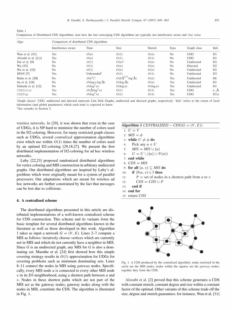
Table 1 presents a comparison of the various distributed CDSalgorithms known in the literature. Algorithms CDSColor andCDSTop, the two distributed algorithms presented in this work,are also featured in the table. The columns from left to rightcorrespond to the following aspects of the algorithms, respec-tively: the name of the algorithm, whether the algorithm ex-plicitly takes into account the loss of messages due to wirelessinterference, the time complexity of the algorithm, the worstcase approximation ratio of the size of the CDS, the worst casestretch of the CDS, whether the CDS algorithm requires thenetwork to be synchronized, the graph classes to which theguarantees of the CDS algorithm apply, and the informationrequired at each node during the execution of the algorithm.We remark that Dai et al. [9] present a constant upper boundon the size ratio of their distributed CDS algorithm for ran-dom UDGs. The SPAN algorithm [7] is implemented over the802.11 MAC layer protocol and hence the worst case conver-gence time for SPAN is not known (and assumed to be un-bounded). We also note that the algorithm of Kuhn et al. [20]takes as input a value k, runs in time O(k2) and yields a dom-inating set of expected size O(k�2/k log �) times the optimal.A preliminary version of the techniques developed in this paperalso appears in Parthasarathy et al. [26]. As the table indicates,our distributed CDS algorithms are the first to incorporate wire-less interference and converge in polylogarithmic time, albeitfor synchronous networks.
Kuhn et al. [19] and Moscibroda et al. [25] propose fastinterference-aware distributed algorithms for wireless net-works; the proposed algorithms construct a dominating set and
a MIS and have time complexities, O(log2 n) and O(log3 n
log log n),
respectively. Significantly, both these papers assume an asyn-chronous quasi-UDG model for the ad hoc network and as-sume that the network nodes have no information about theirlocal neighborhood and do not possess a reliable collisiondetection mechanism (i.e., nodes cannot distinguish betweencollision and lack of transmission). However, unlike the tech-niques presented in this work, both these papers deal onlywith clustering the network and do not deal with obtaininga connected substructure of the network. We believe that thealgorithmic techniques presented here and those of [19] and[25] are complementary to each other and combining theseapproaches for developing faster CDS algorithms under morestringent network models merits future investigation.
D2-coloring is a problem with natural applications toconflict-free broadcast scheduling and channel assignment in
R. Gandhi, S. Parthasarathy / J. Parallel Distrib. Comput. 67 (2007) 848–862 851
Table 1Comparison of Distributed CDS Algorithms: note how the fast converging CDS algorithms are typically not interference aware and vice versa
Algo Comparison of distributed CDS algorithms
Interference aware Time Size Stretch Sync Graph class Info
Wan et al. [31] Yes O(n) O(1) O(n) No UDG D1Alzoubi et al. [2,1] Yes O(n) O(1) O(1) No UDG D1Dai et al. [9] No O(1) O(n)∗ O(n) No Undirected D2Wu [33] No O(1) O(n) O(n) No Directed D2Wu et al. [32] No O(1) O(n) O(n) No Undirected D2SPAN [7] Yes Unbounded∗ O(1) O(1) No Undirected D3
Kuhn et al. [20] No O(k2)∗ O(k�2/klog�) O(n) Yes Undirected Dk
Jia et al. [16] No O(log n log�) O(log�) O(n) Yes Undirected D1Dubashi et al. [12] No O(log2 n) O(log n) O(log n) Yes Undirected D1CDSColor Yes O(� log2 n) O(1) O(1) Yes UDG n,�CDSTop Yes O(log2 n) O(1) O(1) Yes UDG D3,n
‘Graph classes’ UDG, undirected and directed represent Unit Disk Graphs, undirected and directed graphs, respectively. ‘Info’ refers to the extent of localinformation (and global parameters) which each node is expected to know.∗See remarks in Section 3.
wireless networks. In [29], it was shown that even in the caseof UDGs, it is NP-hard to minimize the number of colors usedin the D2-coloring. However, for many restricted graph classessuch as UDGs, several centralized approximation algorithmsexist which use within O(1) times the number of colors usedby an optimal D2-coloring [29,18,27]. We present the firstdistributed implementation of D2-coloring for ad hoc wirelessnetworks.
Luby [22,23] proposed randomized distributed algorithmsfor vertex coloring and MIS construction in arbitrary undirectedgraphs. Our distributed algorithms are inspired by Luby’s al-gorithms which were originally meant for a system of parallelprocessors. Our adaptations which are meant for wireless adhoc networks are further constrained by the fact that messagescan be lost due to collisions.
4. A centralized scheme
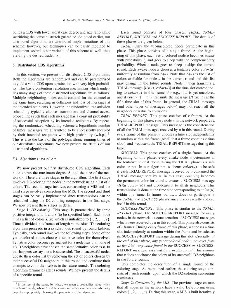
The distributed algorithms presented in this article are dis-tributed implementations of a well-known centralized schemefor CDS construction. This scheme and its variants form thebasic template for several distributed algorithms known in theliterature as well as those developed in this work. Algorithm1 takes as input a network G = (V , E). Lines 2–7 compute aMIS as follows: iteratively choose vertices which are currentlynot in MIS and which do not currently have a neighbor in MIS.Since G is an undirected graph, any MIS for G is also a dom-inating set. Marathe et al. [24] first showed how this simplecovering strategy results in O(1) approximation for UDGs forcovering problems such as minimum dominating sets. Lines8–11 connect the nodes in MIS using gateway nodes. Specifi-cally, every MIS node u is connected to every other MIS nodev in its D3-neighborhood, using a shortest path between u andv. Nodes in these shortest paths which are not part of theMIS act as the gateway nodes; gateway nodes along with thenodes in MIS, constitute the CDS. The algorithm is illustratedin Fig. 1.
Algorithm 1 CENTRALIZED − CDS(G = (V , E))
1: U = V
2: MIS = �3: while U �= � do4: Pick any u ∈ U
5: MIS = MIS ∪ {u}6: U = U \ ({u} ∪ N(u))
7: end while8: CDS = MIS9: for all {u, v} ⊆ MIS do
10: if D(u, v)�3 then11: P = set of nodes in a shortest path from u to v
12: CDS = CDS ∪ P
13: end if14: end for15: return CDS
Fig. 1. A CDS produced by the centralized algorithm: nodes enclosed in thecircle are the MIS nodes; nodes within the squares are the gateway nodes;together they form the CDS.
Alzoubi et al. [2] proved that this scheme generates a CDSwith constant stretch, constant degree and size within a constantfactor of the optimal. Other variants of this scheme trade off thesize, degree and stretch guarantees: for instance, Wan et al. [31]
852 R. Gandhi, S. Parthasarathy / J. Parallel Distrib. Comput. 67 (2007) 848–862
builds a CDS with lower worst case degree and size ratio whilesacrificing the constant stretch guarantee. As noted earlier, ourdistributed algorithms are distributed implementations of thisscheme; however, our techniques can be easily modified toimplement several other variants of this scheme as well, thusyielding the desired tradeoffs.
5. Distributed CDS algorithms
In this section, we present our distributed CDS algorithms.Both the algorithms are randomized and can be parametrizedto yield a valid CDS upon termination with very high probabil-ity. The basic contention resolution mechanism which under-lies many stages of these distributed algorithms are as follows.Multiple neighboring nodes could contend for the channel atthe same time, resulting in collisions and loss of messages atthe intended recipients. However, the randomized transmissionscheduling typically chooses transmitters and channel accessprobabilities such that each message has a constant probabilityof successful reception by its intended recipients. By repeat-ing the randomized scheduling scheme a logarithmic numberof times, messages are guaranteed to be successfully receivedby their intended recipients with high probability (w.h.p.). 3
This is also the basis of the polylogarithmic running times ofour distributed algorithms. We now present the details of ourdistributed algorithms.
5.1. Algorithm CDSColor
We now present our first distributed CDS algorithm. Eachnode knows the maximum degree �, and the size of the net-work n. There are three stages in the algorithm. The first stageinvolves D2-coloring the nodes in the network using a list of ccolors. The second stage involves constructing a MIS and thethird stage involves connecting the MIS. The second and thirdstages can be easily implemented since transmissions can bescheduled using the D2-coloring computed in the first stage.We now present these stages in detail.
Stage 1: D2-coloring. This stage is parametrized by threepositive integers: c, t, and r (to be specified later). Each nodeu has a list of colors L(u) which is initialized to {1, 2, . . . , c}.Time is divided into frames of length c time slots. The coloringalgorithm proceeds in a synchronous round by round fashion.Typically, each round involves the following steps. Some of theyet-uncolored nodes choose a tentative color for themselves.Tentative color becomes permanent for a node, say v, if none ofv’s D2-neighbors have chosen the same tentative color as v. Inthis happens we say that v is successful. The unsuccessful nodesupdate their color list by removing the set of colors chosen bytheir successful D2-neighbors in this round and continue theirattempts to color themselves in the future rounds. The coloringalgorithm terminates after t rounds. We now present the detailsof a specific round.
3 In the rest of the paper, by w.h.p., we mean a probability value whichis at least 1 − 1
n� , where � > 0 is a constant which can be made arbitrarilylarge by appropriately choosing the parameters of the algorithm.
Each round consists of four phases: TRIAL, TRIAL-REPORT , SUCCESS and SUCCESS-REPORT . The details ofthese phases are given below.
TRIAL: Only the yet-uncolored nodes participate in thisphase. This phase consists of a single frame. At the begin-ning of this phase, each yet-uncolored node u becomes awakewith probability 1
2 and goes to sleep with the complementaryprobability. When a node goes to sleep it skips the currentround. Each awake node u chooses a tentative color color(u)
uniformly at random from L(u). Note that L(u) is the list ofcolors available for node u in the current round and this listmay change in the future rounds. Node u then transmits aTRIAL message {ID(u), color(u)} at the time slot correspond-ing to color(u) in this frame: for e.g., if u is yet-uncoloredand if color(u) = 5, u transmits the message {ID(u), 5} at thefifth time slot of this frame. In general, the TRIAL message(and other types of messages below) may not reach all theneighbors of u due to collisions.
TRIAL-REPORT : This phase consists of r frames. At thebeginning of this phase, every node u in the network prepares aTRIAL-REPORT message. This message is the concatenationof all the TRIAL messages received by u in this round. Duringevery frame of this phase, u chooses a time slot independentlyat random within the frame (recall that a frame contains c timeslots), and broadcasts the TRIAL-REPORT message during thistime.
SUCCESS: This phase consists of a single frame. At thebeginning of this phase, every awake node u determines ifthe tentative color it chose during the TRIAL phase is a safecolor or not. In our algorithm, u deems color(u) to be safeif each TRIAL-REPORT message received by u contained theTRIAL message sent by u. In this case, color(u) becomesthe permanent color for u and u creates a SUCCESS message{ID(u), color(u)} and broadcasts it to all its neighbors. Thistransmission is done at the time slot corresponding to color(u)
within this frame. In future rounds, u does not participate inthe TRIAL and SUCCESS phases since it successfully coloreditself in this round.
SUCCESS-REPORT : This phase is similar to the TRIAL-REPORT phase. The SUCCESS-REPORT message for everynode u in the network is a concatenation of SUCCESS messageswhich were received by u in this round. This phase also consistsof r frames. During every frame of this phase, u chooses a timeslot independently at random within the frame and broadcastsits SUCCESS-REPORT message during this slot. Crucially, atthe end of this phase, any yet-uncolored node v removes fromits list L(v), any color found in the SUCCESS or SUCCESS-REPORT messages received by v in this round. This ensuresthat v does not choose the colors of its successful D2-neighborsin the future rounds.
This completes the description of a single round of thecoloring stage. As mentioned earlier, the coloring stage con-sists of t such rounds, upon which the D2-coloring subroutineterminates.
Stage 2: Constructing the MIS. The previous stage ensuresthat all nodes in the network have a valid D2-coloring usingcolors {1, 2, . . . , c}. During this stage, a MIS is built iteratively

R. Gandhi, S. Parthasarathy / J. Parallel Distrib. Comput. 67 (2007) 848–862 853
in c time slots. During slot i, all nodes belonging to color classi attempt to join the MIS. A node joins the MIS if and onlyif none of its neighbors are currently part of the MIS. Afterjoining the MIS, the node broadcasts a message to its neighborsindicating that it joined the MIS. Nodes transmitting during thesame time slot belong to the same color class and hence do notshare a common neighbor. Clearly, this stage requires exactlyc time steps.
Stage 3: Connecting the MIS. This stage requires six phases.Each phase is one frame long and a single frame is of length c.As in stage two, nodes transmit only during the time slot cor-responding to their D2-color. During the first phase, all MISnodes transmit a PHASE-1 message. This message just con-sists of the node’s ID. In the second phase, any node u whichreceived a PHASE-1 message, transmits a PHASE-2 message.This message is a concatenation of ID(u) and all the PHASE-1messages received by u. In the third phase, any node u whichreceived a PHASE-2 message, transmits a PHASE-3 message.This message is a concatenation of ID(u) and all the PHASE-2messages received by u.
By the end of the third phase, every MIS node u knows ev-ery other MIS node v in its D3-neighborhood. Node u alsoknows all paths of length at most three between itself and v.Node u constructs a PHASE-4 message as follows: for everyother MIS node v such that v is in its D3-neighborhood andID(v) > ID(u), u chooses a path of length at most three hopsbetween itself and v. It adds this information to its PHASE-4message. All MIS nodes transmit a PHASE-4 message dur-ing the fourth phase. Every node u which received a PHASE-4message transmits a PHASE-5 message. This message is a con-catenation of all the PHASE-4 messages received by u. Finally,every node u which received a PHASE-5 message transmitsa PHASE-6 message. This message is a concatenation of allthe PHASE-5 messages received by u. By the end of thisstage, any MIS node u knows the path between itself and anyother MIS node v which is in its D3-neighborhood. In addi-tion, any node w which is not part of the MIS, knows if it ispart of the final CDS or not. All three stages are illustratedin Fig. 2.
We now specify the values for the various parameters in thealgorithm, which completes the description of the algorithm:c = k4�, t = k5 log n, and r = k6 log n, where k4, k5 and k6are suitable constants.
5.2. Analysis of algorithm CDSColor
Theorem 1. The running time of the algorithm is O(� log2 n).
Proof. The first stage consists of t rounds, each of which con-sists of 2(r + 1) frames. The second and third stages consist of1 and 6 frames, respectively. Hence, the total number of framesis O(tr) = O(log2 n). All frames are of length c = O(�).Hence, the running time is O(� log2 n). �
The following definition and claims are useful for the rest ofthe analysis.
Definition. Let S be a set of disks in the plane. Let C be adisk in the plane. For any disk s, we let s denote both the diskand the set of points contained within the disk. We say thatS is a covering for C iff the following hold: 1. C ⊆ ⋃
s∈S s,2. ∀s ∈ S, s ∩ C �= �, 3. ∀{s1, s2} ⊆ S, the center of s1 liesoutside the center of s2 and vice versa. We state the followingsimple claim from geometry.
Claim 2. Let S be a set of disks of radius r1 and C be a diskof radius r2. Let S be a covering for C. Then, |S|�k0(
r1+r2r1
)2,where k0 is a constant. In addition, such a covering alwaysexists.
We use the above claim to prove the following lemma.
Lemma 3. Let G = (V , E) be a UDG with maximum degree�. Let C be a disk of radius r� 1
2 . The number of nodes of Vwhich lie within C is at most 4k0r
2(� + 1).
Proof. Let S be a set of disks of radius 12 which cover C. The
maximum number of nodes which lie within any disk in S isat most � + 1 (since such nodes form a clique). The numberof disks in S by Claim 2 is at most 4k0r
2. Hence, the lemmafollows. �
Theorem 4. All messages in the algorithm require at mostO(� log n) bits.
Proof. The TRIAL and SUCCESS messages transmitted bya node u are of the form {ID(u), color(u)}. The PHASE-1 and PHASE-4 messages are of the form {ID(u)}. ThePHASE-2 (PHASE-5) message is a concatenation of anode’s ID and the PHASE-1 (PHASE-4) messages trans-mitted by its one-hop MIS neighbors. All one-hop MISneighbors are within a disk of radius one and the subgraphinduced by the MIS nodes is a UDG with maximum de-gree zero. Hence, by Lemma 3, there can be at most O(1)
MIS nodes within a disk of radius 1. Hence PHASE-1,PHASE-2, PHASE-4, and PHASE-5 messages require at mostO(log n) bits. All other messages are a concatenation of atmost � messages of the previous types and hence require atmost O(� log n) bits. �
Theorem 5. The total number of messages transmitted by thealgorithm is at most O(n log2 n).
Proof. There are O(log2 n) frames in the algorithm. Eachnode transmits at most once per frame. Hence the theoremfollows. �
We now prove the following lemmas which pertain to thecorrectness of the algorithm.
Lemma 6. Let u be a node which is yet-uncolored at the begin-ning of a round i. Let Li(u) be the color-list of u in the begin-ning of round i. Let S be the set of D2-neighbors of u which are
854 R. Gandhi, S. Parthasarathy / J. Parallel Distrib. Comput. 67 (2007) 848–862
b
1 23
a
Fig. 2. Algorithm CDSColor: subfigures (a) and (b) represent the TRIAL and SUCCESS phases of the D2-coloring stage; squares, hexagons and circlesrepresent three distinct colors; solid enclosures represent permanent colors and dotted enclosures represent tentative colors; nodes that are not enclosed are notawake; note how two D2-neighbors enclosed in dotted squares are unsuccessful in subfigure (b). Subfigures (c) and (d) represent the MIS construction phase:nodes in (d) with black fillings are the MIS nodes; all nodes enclosed within circles join the MIS first; after this, only one node within a square can join theMIS; other colors are not shown for clarity. Subfigure (e) shows how the MIS nodes get connected; nodes along the dotted lines 1, 2, and 3 know about theMIS node ‘a’ through PHASE-1, PHASE-2 and PHASE-3 messages; PHASES-4, 5, and 6 are analogous.
yet-uncolored at the beginning of round i. Then, |Li(u)|� |S|+1. In particular, the color-list of u is never empty before u issuccessfully colored.
Proof. Recall that c = k4� is the initial size of the color-listfor all nodes. Lemma 3 implies that the maximum number ofD2-neighbors for any node is at most 16k0(� + 1). Let theconstant k4 be chosen such that k4 > 32k0. Hence each nodeinitially has a list of c colors which is strictly greater than thenumber of its D2-neighbors. A node removes at most one colorfor each of its successful D2-neighbors in any round. Hence,the lemma follows. �
The above lemma ensures that the TRIAL phase is welldefined: i.e., no node has an empty color-list before it is success-fully colored. The following lemma ensures that the TRIAL-REPORT and SUCCESS-REPORT phases are executedcorrectly, resulting in a valid D2-coloring of vertices.
Lemma 7. Let u be a node which transmits TRIAL(SUCCESS)-REPORT messages during a fixed round i. Let v be a fixedneighbor of u. Consider the event that v does not receive evena single TRIAL(SUCCESS)-REPORT message collision-freefrom u during round i. The probability of this event occurringis at most 1
n� .
R. Gandhi, S. Parthasarathy / J. Parallel Distrib. Comput. 67 (2007) 848–862 855
Proof. Consider the event that the TRIAL-REPORT messagetransmitted by node u in a particular frame is not received bynode v. We now compute the probability of this event. Recallthat u (and any other node) chooses a time slot independentlyat random within a frame and transmits the TRIAL-REPORTmessage. Let Tx,j denote the time slot chosen by a node x inframe j. Let S = {v}∪N(v)\{u}. Note that S is the set of nodeswhich could interfere with u’s transmission and cause collisionat v. Specifically, node v will not receive u’s message duringframe j only if there exists a node x ∈ S such that Tx,j = Tu,j .We have,
Pr[∃x ∈ S, Tx,j = Tu,j ] = 1 − Pr[∀x ∈ S, Tx,j �= Tu,j ]= 1 −
∏x∈S
Pr[Tx,j �= Tu,j ]
= 1 −∏x∈S
(1 − 1
c
)
= 1 −(
1 − 1
c
)|S|
� 1 −(
1 − 1
c
)�
.
Since c = k4�, by letting k4 > 1, we have
(1 − 1
c
)�
� 1
4.
Hence, Pr[∃x ∈ S, Tx,j = Tu,j ]� 34 .
In order for v not to get even a single TRIAL-REPORT messageof u, the above event (∃x ∈ S, Tx,j = Tu,j ) should occur forall frames j ∈ {1, . . . , r} in the TRIAL-REPORT phase. Thus,
Pr[v not receiving any TRIAL-REPORT from u] � ( 34 )r
= ( 34 )k6 log n
= 1
n�.
Here, � is a constant which can be made arbitrarily high bychoosing an appropriate value of k6. This completes the proofof the lemma. �
Lemma 8. Let u, v be any fixed pair of D2-neighbors. Whenthe algorithm terminates, u and v have the same color with atmost a negligible low probability of 1
n� , where � is a constantwhich can be made arbitrarily high.
Proof. Assume that u and v have been successfully coloredwith the color z, during rounds i and j, respectively. W.l.o.g.,let i�j . There are two possible cases.
The first case occurs when u and v are neighbors of eachother. In this case, since u is colored successfully in round i, noneighbor of u and no neighbor v (except u), chose the tentativecolor z during round i (otherwise, the TRIAL-REPORT of v
would not have contained the TRIAL of u, and u would not havedeemed itself successful). This also implies that v received theSUCCESS message of u during round i collision-free. Hence, vwould have removed color z from its list during round i, leadingto a contradiction.
The second case occurs when u and v are not neighborsof each other. In this case, there exists a node x which is aneighbor of both u and v. By the same arguments as above, xreceives the TRIAL and SUCCESS messages of u during roundi, collision-free. Hence, the TRIAL-REPORT and SUCCESS-REPORT messages of x in round i, contains the color z. Node v
would deem z as its permanent color during round j = i, onlyif it did not receive any TRIAL-REPORT messages transmittedby x in round i. Node v would choose color z during a round j >
i, only if it did not receive any SUCCESS-REPORT messagestransmitted by x in round i. By Lemma 7, both these eventsoccur with the negligible low probability of 1
n� , where � is aconstant which can be made arbitrarily high. This completesthe proof of the lemma. �
Lemma 9. Consider the final colors of all the nodes after theD2-coloring algorithm terminates. No two nodes which are D2-neighbors of each other have the same color, w.h.p.
Proof. There are at most n2 pairs of neighbors. By Lemma 8and using the union bound, the probability of any of these pairshaving the same color is at most n2( 1
n)�. Hence, the probability
of no pair of neighbors having the same D2-color is at least1 − 1
n�−2 , where � is a constant which can be made arbitrarilyhigh. This completes the proof of the lemma. �
Lemma 10. Let u be a yet-uncolored node at the beginning ofa particular round i. Let S(u, i) denote the event that u wassuccessfully colored during round i. Then, Pr[S(u, i)]� 3
4 .
Proof. Recall that Li(u) is the color-list of u in the begin-ning of round i. Let N be the set of D2-neighbors of u whichare yet-uncolored in the beginning of round i. Let A(x) de-note the event that node x is awake during round i. Let C(x, z)
denote the event that node x chose the tentative color z dur-ing the TRIAL phase of round i. We note that for the eventS(u, i) to occur, at least one of the following two events shouldoccur:
1. A(u): u was not awake in round i. This event occurs withprobability 1
2 .2. ∃(x ∈ N, z ∈ Li(u)) such that C(x, z) and C(u, z): Some
D2-neighbor of u choose the same color as u. We denotethis event as F(u).
We now compute Pr[F(u)]. We first note that for any node x,the probability that it chooses any color from its list is at most12 , since it needs to be awake before choosing a color. In addi-tion, Pr[C(x, z)]� 1
2|Li(x)| , since x chooses a color uniformly

856 R. Gandhi, S. Parthasarathy / J. Parallel Distrib. Comput. 67 (2007) 848–862
at random from its list. We have,
Pr[F(u)] =∑
z∈Li(u)
Pr[C(u, z)](∑
x∈N
Pr[C(x, z)])
= 1
2|Li(u)|∑
z∈Li(u)
(∑x∈N
Pr[C(x, z)])
= 1
2|Li(u)|∑x∈N
⎛⎝ ∑
z∈Li(u)
Pr[C(x, z)]⎞⎠
� 1
2|Li(u)|∑x∈N
1
2
� |N |4|Li(u)| .
By Lemma 6, |Li(u)|� |N | + 1. Hence, the above probabilityis at most 1
4 . Hence, we have
Pr[S(u, i)]� 12 + 1
4 ,
which completes the proof of the lemma. �
Lemma 11. When D2-coloring algorithm terminates, w.h.p.all nodes are successfully colored.
Proof. By Lemma 10, the probability of a particular node uremaining yet-uncolored after the algorithm terminates is atmost ( 3
4 )t = ( 34 )k5 log n = 1
n� . Hence, the probability of somenode remaining yet-uncolored after the algorithm terminates isat most n
n� = 1n�−1 . Here, � is a constant which can be made
arbitrarily high by choosing the appropriate value of k5. Thisconcludes the proof of the lemma. �
Theorem 12. The first stage computes a valid D2-coloringw.h.p.
Proof. Lemmas 9 and 11 together yield this theorem. �
Theorem 13. The second and third stages compute a valid MISand CDS, respectively, w.h.p.
Proof. Observe that if the first stage produces a valid D2-coloring, then no packets are lost due to collision and the sec-ond and third stages are executed correctly. By Theorem 12,the first stage computes a valid D2-coloring w.h.p. Hence thistheorem follows. �
5.3. Algorithm CDSTop
We now describe our distributed CDS algorithm based onneighborhood topology information. Each node is assumedto have knowledge of its D3-topology, i.e., nodes in its three
hop neighborhood and the edges between these nodes. Thealgorithm comprises of two stages. An MIS is constructed inthe first stage and it is connected in the second stage. Boththe first and the second stage of the algorithm involve theuse of the collision-free broadcasting algorithm of Gandhiet al. [13], to broadcast messages to D2- and D3-neighborhoods,respectively: the broadcast subroutine utilizes the D2- andD3-topology information to create a collision-free broadcastschedule. We now present the details of these stages below.
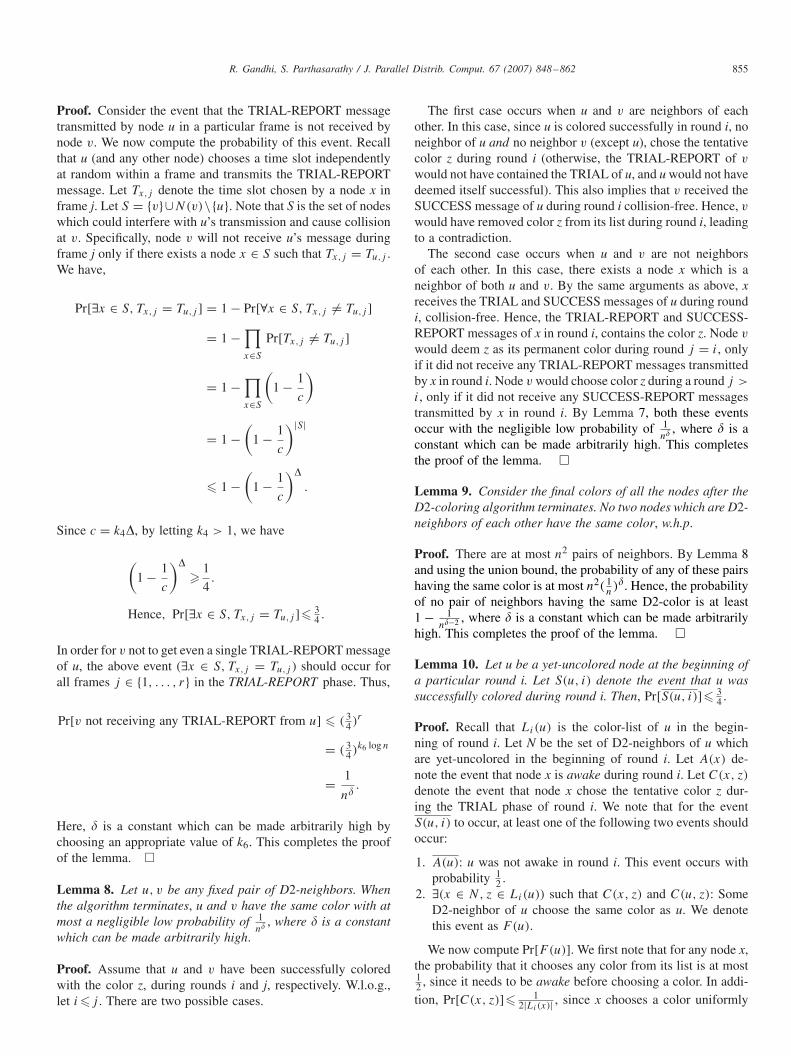
Stage 1: Constructing the MIS. This stage proceeds in a syn-chronous round by round fashion. The MIS is initially empty.Typically, some nodes are successful at the end of each round.A node is deemed successful if either the node joins the MISor one of its neighbors joins the MIS. Successful nodes do notparticipate in the future rounds, while the yet-unsuccessful onescontinue their attempts in the future rounds. The MIS construc-tion terminates after t rounds.
During this stage, each node u maintains a status variablewhich is defined as follows: status(u) = in iff u has joined theMIS; status(u) = out if any neighbor of u has joined the MIS;status(u) = unsure otherwise. All nodes are initially unsure andbecome in or out of MIS during the course of the algorithm.Let Vi be the set of nodes whose status is unsure at the end ofround i − 1. For any node u ∈ Vi , let Ni(u) = N(u) ∩ Vi . LetMISi be the set of nodes which join MIS in round i.
There are four phases in each round of the first stage:TRIAL, CANDIDATE-REPORT , JOIN , and PREPARE. Wenow present the details of these phases for a particular round i.
TRIAL: In this phase, each unsure node decides if it is a can-didate for MISi . Specifically, each unsure node u chooses itselfto be a candidate for joining MISi , with probability 1
2(|Ni(u)|+1).
Node u will not be a candidate in this round with the com-plement probability. This phase does not involve any messagetransmissions.
CANDIDATE-REPORT : This phase ensures that each nodeknows if there is a neighbor who is a candidate. This step con-sists of p time frames, each frame consisting of two slots. Dur-ing every frame of this phase, each candidate node choosesone of the two slots independently at random and broadcastsa CANDIDATE message. Any node which receives a CAN-DIDATE message or experiences collision during this phase,knows that there is a neighboring candidate; otherwise it as-sumes that there is no neighboring candidate.
JOIN : This phase requires a single time slot. In this phase,some unsure nodes become either in or out. How should a can-didate decide if it should join MISi (become in)? A candidatejoins MISi if none of its neighbors are candidates for MISi ,i.e., if it did not receive a CANDIDATE message during theprevious phase. All nodes who joined MISi transmit a JOINmessage. The unsure nodes which receive a JOIN message orexperience collision, change their status to out. Other unsurenodes do not change their status.
PREPARE: Each unsure node u computes Ni+1(u) at the endof this phase. This phase consists of p time frames. Each frameis further subdivided into � subframes of length c. During everyframe of this phase, each node in MISi , chooses independentlyat random, one of the � subframes. During this subframe, it

R. Gandhi, S. Parthasarathy / J. Parallel Distrib. Comput. 67 (2007) 848–862 857
Fig. 3. Algorithm CDSTop: subfigures (a), (b), and (c) show the MIS construction phase: nodes filled with the pattern are unsure nodes; nodes within thedotted circles in (b) are the candidate nodes; in subfigure (c), nodes with black fillings are in the MIS and nodes with white fillings are out of the MIS.Subfigure (d) shows the final MIS; note the three-hop broadcast tree rooted at the encircled MIS node; such three-hop broadcast trees are employed by MISnodes to inform and connect to other MIS nodes within the three-hop neighborhood.
broadcasts a PREPARE message using the algorithm in [13] toits D2-neighbors. The length of the subframe, c is the numberof time slots required by [13] to transmit a message from a nodeto its D2-neighbors. The PREPARE message broadcast by anode simply consists of its ID. By the end of this phase, everyunsure node knows all the nodes in its D2-neighborhood whichjoined MISi . Since it knows its D3 (and hence D2) topology,it can easily compute the value Ni+1(u). Note that, since themessage is being broadcast to the two-hop neighborhood, thebroadcast algorithm guarantees that c is at most a constant [13].
Stage 2: Connecting the MIS. In this phase the MIS computedin the previous stage is connected using intermediate nodes.Specifically, every MIS node connects itself to every other MISnode which is at most three hops away. This stage consistsof two phases: HELLO and CONNECT . We now present thedetails of these phases.
HELLO: This phase is similar to the PREPARE phase in thefirst stage. The objective of this phase is for each MIS nodeto announce itself to other MIS nodes in its D3-neighborhood.This phase consists of p frames, where each frame is subdi-vided into �′ subframes of length c′. During every frame ofthis phase, each node u ∈ MIS node selects independentlyat random, one of the �′ subframes. During this subframe, ubroadcasts a HELLO message using the algorithm in [13] toits D3-neighborhood. By the end of this phase, each MIS nodeknows any other MIS node in its D3-neighborhood.
CONNECT : This phase is similar to the HELLO phase.The only difference arises in the contents of the CONNECTmessage. Each node u ∈ MIS prepares its CONNECTmessage as follows. For every node v ∈ MIS such that v
is in its D3-neighborhood and ID(v) > ID(u), the CON-NECT message of u contains the tuple {ID(v), u�v}. u�v
is the shortest path between u and v. As mentioned ear-lier, CONNECT messages are broadcast in the same wayas the HELLO messages. In general, intermediate nodeswhich are not part of the MIS may join the CDS, sincethey could be a part of the shortest path between two MISnodes.
We complete the description of our topology based dis-tributed CDS algorithm by specifying the values of the variousparameters involved: we let p = k7 log n and t = k8 log n. Welet � and �′ be the maximum number of MIS nodes in the D2-and D3-neighborhoods of any node, respectively: these valuesare fixed constants [13]. Let c and c′ be the maximum number oftime slots required by the broadcast algorithm [13] to broadcasta message to the D2- and D3-neighborhoods of a node, respec-tively: both these values are fixed constants as well [13]. Due tolack of space, we state only the main claim pertaining to the per-formance analysis of our algorithm here. The detailed proof ofthis claim involves several subtle probabilistic and geometric ar-guments; the reader is referred to Fig. 3 for an illustration of thealgorithm.

858 R. Gandhi, S. Parthasarathy / J. Parallel Distrib. Comput. 67 (2007) 848–862
5.4. Analysis of algorithm CDSTop
Theorem 14. The running time of the algorithm is O(log2 n).
Proof. The first stage consists of t rounds, each of which con-sists of (2p + 1 + p�c) slots. The second and third stages to-gether consist of 2p frames, each of which consists of (�′c′)slots. Since �, �′, c, and c′ are constants, the running time isO(tp) = O(log2 n). �
Theorem 15. All messages transmitted in the algorithm re-quire at most O(log n) bits.
Proof. The CANDIDATE, JOIN and PREPARE messages justconsist of a node’s ID. The HELLO and CONNECT messagestransmitted from an MIS node u to another MIS node v justconsists of ID’s of u, v, and at most two intermediate nodes inthe path between u and v. Hence all these messages require atmost O(log n) bits. �
The following lemmas pertain to the correctness of the var-ious phases in the algorithm.
Lemma 16. Consider a candidate node u during a particularround i of the algorithm. Consider a neighbor v of u. Nodev either receives a CANDIDATE message or experiences col-lision w.h.p. during the CANDIDATE-REPORT phase of thisround.
Proof. Recall that the CANDIDATE-REPORT phase consistsof p frames each consisting of two time slots. Let A(u, v, j)
denote the event that both u and v chose the same time slot totransmit their CANDIDATE messages during frame j. Nodev will not receive u’s CANDIDATE message and not expe-rience collision during frame j only if A(u, v, j) occurs. Ifv is not a candidate during round i, then Pr[A(u, v, j)] =0. Else, Pr[A(u, v, j)] = 1
2 . Node v will not receive u’sCANDIDATE message or experience collision during eachof the p frames in the phase, if the event
∧p
j=1 A(u, v, j)
occurs.
Pr
⎡⎣ p∧
j=1
A(u, v, j)
⎤⎦ � 1
2p
= 1
2k7 log n
= 1
n�.
Here, � can be made arbitrarily high by choosing an appropriatevalue of k7. �
Lemma 17. Consider a round i and a node u ∈ MISi . Con-sider a D2-neighbor v of u. v receives (at least one of) thePREPARE message transmitted by u collision-free w.h.p. dur-ing the PREPARE phase of round i.
Proof. Recall that the PREPARE phase is divided into p frames,each of which is divided into � subframes, where the con-stant � is the maximum number of MIS nodes in the D3-neighborhood of any node. Let F(u, j) denote the subframe offrame j during which u broadcast its PREPARE message to itsD2-neighborhood. Let S denote the D3-neighborhood of v. Ifv does not receive u’s PREPARE message during the subframeF(u, j) of frame j, then there exists w ∈ S \ {u} such that theevent F(w, j) = F(u, j) occurred.
Pr[∃w ∈ S \ {u}F(w, j) = F(u, j)]= 1 − Pr[∀w ∈ S \ {u}F(w, j) �= F(u, j)]= 1 −
∏w∈S\{u}
Pr[F(w, j) �= F(u, j)]
= 1 −∏
w∈S\{u}
(1 − 1
�
)
= 1 −(
1 − 1
�
)|S|−1
= 1 −(
1 − 1
�
)�−1
�1 − 1
e.
Let B(u, v, j) denote the bad event that v does not receive u’sprepare message during frame j. The above inequalities implyPr[B(u, v, j)]�1− 1
e. Node v will not receive any of the PRE-
PARE messages transmitted by u if the event∧p
j=1 B(u, v, j)
occurs,
Pr
⎡⎣ p∧
j=1
B(u, v, j)
⎤⎦ =
p∏j=1
Pr[A(u, v, j)]
�(
1 − 1
e
)p
�(
1 − 1
e
)k7 log n
� 1
n�.
Here, � is a constant which can be made arbitrarily large bychoosing an appropriate value of k7. This completes the proofof the lemma. �
Lemma 18. Consider a node u ∈ MISi and a D3-neighborv of u. Node v receives (at least one of) the HELLO (CON-NECT) messages transmitted by u collision-free w.h.p. duringthe HELLO (CONNECT) phase of the second stage.
Proof. The proof of this lemma is identical to the proofof Lemma 17, except for the following differences: the
R. Gandhi, S. Parthasarathy / J. Parallel Distrib. Comput. 67 (2007) 848–862 859
PREPARE message is broadcast to D2-neighborhood of anode, whereas the HELLO (CONNECT) message is broadcastto the D3-neighborhood. The constants � and c in the proofof Lemma 17 are replaced by the constants �′ and c′ in thisproof. �
Lemma 19. Consider the following bad events:1. During the CANDIDATE-REPORT phase of some round of
the first stage, a neighbor of some candidate node did notreceive any of the CANDIDATE messages transmitted bythe candidate node and did not experience collision.
2. During some round of the algorithm, a D2-neighbor of someMIS node did not receive any of the PREPARE messagestransmitted by the MIS node.
3. During some HELLO (CONNECT) phase of the secondstage, a D3-neighbor of some MIS node did not receive anyof the HELLO (CONNECT) messages transmitted by theMIS node w.h.p.
W.h.p., none of the above bad events happen during the courseof the algorithm.
Proof. The proof for all three bad events stated above are sim-ilar and uses the union bound. By Lemma 16, during a fixedround i, for a fixed candidate node u and for a fixed neighborv of u, the probability of v not receiving any of u’s CANDI-DATE messages and not experiencing collision is during roundi is at most 1
� . There are O(n2) pairs of neighbors and O(log n)
rounds. The probability of the bad event occurring during atleast once during any of these rounds for any pair of neigh-
bors is at most O(n2 log n
n� ) = O( 1n� ), where � (and hence �)
can be made arbitrarily high. Similarly, by Lemmas 17 and 18,and by arguments which are essentially the same as the above,the second and third bad events occur with probability at mostO( 1
n� ), where � can be made arbitrarily high. Hence, none ofthe three bad events occur w.h.p. �
Lemma 20. The MIS computed at the end of the first stage isan independent set w.h.p.
Proof. The MIS computed at the end of the first stage willnot be an independent set, only if one of the first two badevents in Lemma 19 occur. These events occur with negligibleprobability. Hence the lemma follows. �
Lemma 21. If MIS is a maximal independent set, then the sec-ond stage computes a valid CDS w.h.p.
Proof. Assume that the first stage computes an MIS which isa valid maximal independent set. Then the CDS computed inthe second stage will not be valid, only if the third bad eventin Lemma 19 occurs. Lemma 19 states that this event doesnot occur during the second stage, w.h.p. Hence the lemmafollows. �
We now prove that the MIS is also maximal, i.e., all nodes areeither in or out of the MIS after the first stage. Let H be a disk ofradius 1
2 . Let V (H) denote the set of nodes which lie within H.
Consider a fixed round i during the first stage of the algorithm.Let C(u, i) denote the event that node u was a candidate forMISi . Recall that Vi is the set of unsure nodes before round i.Let Xi(H) be the random variable which denotes the numberof candidate nodes within disk H. Let Vi(H)
.= V (H)⋂
Vi .The following lemmas hold.
Lemma 22. Pr[Xi(H) > 0]� 12 .
Proof. Since H is a disk of radius 12 , any two nodes within H
are neighbors of each other. Hence,
E[Xi(H)] =∑
u∈Vi(H)
Pr[C(u, i)]
=∑
u∈Vi(H)
1
2(|Ni(u)| + 1)
�∑
u∈Vi(H)
1
2(|Vi(H)|)
= 12 . �
Lemma 23. Let v ∈ Vi(H) be a candidate for MISi . Then,Pr[Xi(H)�2|C(v, i)]� 1
2 . Hence, Pr[Xi(H) = 1|C(v, i)]� 1
2 . Since this holds for any v ∈ Vi(H), Pr[Xi(H) = 1|Xi(H)
�1]� 12 .
Proof. Let Yi(H) be the random variable which denotesthe number of candidates in V(H) \ {v}. Clearly, Xi(H) =Yi(H) + 1,
Pr[Xi(H)�2|C(v, i)] = Pr[Yi(H)�1|C(v, i)]= Pr[Yi(H) > 0|C(v, i)]� E[Yi(H)|C(v, i)]=
∑u∈Vi(H)\{v}
Pr[C(u, i)|C(v, i)]
=∑
u∈Vi(H)\{v}Pr[C(u, i)]
=∑
u∈Vi(H)\{v}
1
2(|Ni(u)| + 1)
�∑
u∈Vi(H)\{v}
1
2(|Vi(H)|)
� 12 . �
For the rest of the analysis, let S be a set of disks of radius12 which cover the disk of unit radius centered at u. Let H ∈ S
contain node u.

860 R. Gandhi, S. Parthasarathy / J. Parallel Distrib. Comput. 67 (2007) 848–862
Lemma 24. Pr[u ∈ MISi |C(u, i)]��, where � > 0 is a con-stant.
Proof.
Pr[u ∈ MISi |C(u, i)]� Pr[(Xi(H) = 1) ∧ (∀(s ∈ S \ {H })
(Xi(s) = 0))|C(u, i)]� Pr[(Xi(H) = 1)|C(u, i)]
Pr[(∀(s ∈ S \ {H })(Xi(s) = 0))|C(u, i)]
� 1
2
∏s∈S{H }
Pr[Xi(s) = 0|C(u, i)]
� 1
2
(1
2|S|−1
)
� 1
2|S|
= �.
Claim 2 implies that |S| is O(1). Hence, � > 0 is aconstant. �
Consider the graph F whose vertices are the disks in S,and two vertices H1, H2 are adjacent in F iff there existsnodes u ∈ V (H1) and v ∈ V (H2) such that (u, v) ∈ E.Claim 2 implies that the maximum degree of any nodein F is at most a constant �. We now construct a di-rected forest F = (S, I ) as follows. For every H1 ∈ S, letp(H1) = minu∈Vi(H1) Pr[C(u, i)]. If p(H1) < 1
4|Vi(H1)|�2 ,
then |Ni(u)|�2|Vi(H1)|�2. Hence, there exists H2 adjacentto H1 in F such that |V (H2) ∩ Ni(u)|�2|Vi(H1)|�. We addthe edge (H2, H1) in F . Note that we add at most one in-edgefor every node H ∈ S and if the directed edge (H2, H1) existsin F , then |Vi(H2)| > |Vi(H1)|. Hence F is an out-directedforest. We now prove the following claims.
Claim 25. Let H be a vertex in F and let Children(H) bethe children of H in F . Then, |Vi(H)|�2(
∑H ′∈Children(H)|Vi(H
′)|).
Proof. The number of vertices adjacent to H in F (and F) is atmost �. If (H, H ′) is an edge in F , then |V (H)i |�2�|Vi(H
′)|.Hence, |Vi(H)|
� �2|Vi(H′)|. Since, there are at most � children
of H, the claim follows. �
Claim 26. Let T be a tree in the forest F . Let H be anynode in T . Let Desc(H) denote the descendents of H inT . |Vi(H)|�∑H ′∈Desc(H) |Vi(H
′)|. In particular, this claimholds for the root of the tree T .
Proof. Let Height(H) denote the height of H in the treeT . The leaf nodes have a height of 0. Their parents have a
height of 1 and so on. The proof is by induction on Height(H).
Base Case: Height(H) = 0. In this case, H is a leaf nodeand has no descendents. Hence the claim holds.
Induction Hypothesis: Let the claim hold for all nodes suchthat their height is �h.
Induction Step: We now prove the claim for a node H suchthat Height(H) = h+1. For any H1 ∈ Children(H), by the in-duction hypothesis, |Vi(H1)|�∑H2∈Desc(H1)
|Vi(H2)|. Hence,
|V (H) ∩ Vi | � 2
⎛⎝ ∑
H1∈Children(H)
|Vi(H1)|⎞⎠
�∑
H1∈Children(H)
2|Vi(H1)|
�∑
H1∈Children(H)
⎛⎝|Vi(H1)|
+∑
H2∈Desc(H1)
|Vi(H2)|⎞⎠
=∑
H ′∈Desc(H)
|Vi(H′)|.
This completes the proof of the claim. �
Claim 27. Let T be any tree in the forest F and let H denotethe root of T . Pr[|Xi(H)| > 0]��, where � > 0 is a constant.
Proof. Since H is the root of T , it does not have anyin-edge incident upon it. Hence, for all u ∈ Vi(H),Pr[C(u, i)]� 1
4�2|Vi(H)| . Hence,
Pr[|Xi(H)| > 0] �∑
u∈Vi(H)
Pr[C(u, i)]
�∑
u∈Vi(H)
1
4�2|Vi(H)|
� 1
4�2= �. �
Let Zi ⊆ Vi denote the set of nodes which are candidates forMISi or which have a neighbor who is a candidate for MISi .
Lemma 28. E[|Zi |]�|Vi |, where > 0 is a constant.
Proof. Let T be any tree in the forest F . For any H ′ ∈ T , letZi(H
′) be the set of nodes in Vi(H′) which are candidates for
MISi or which have a neighbor who is a candidate for MISi . Wenow show that
∑H ′inT |Zi(H
′)|��∑
H ′inT |Vi(H′)|, where
� > 0 is a constant. If this holds for every tree in the forest, thenclearly the lemma holds. We now prove the above inequality
R. Gandhi, S. Parthasarathy / J. Parallel Distrib. Comput. 67 (2007) 848–862 861
for T . Let H be the root of T . Since there is no in-edge (H ′, H)
incident upon H, the following holds:
∑H ′∈T
E[|Zi(H′)|] � E[|Zi(H)|]
� |Vi(H)| Pr[|Xi(u) > 0]
� 1
2�∑
H ′∈T|Vi(H
′)|�
�
( ∑H ′∈T
|Vi(H′)|)
.
This concludes the proof of the lemma. �
Let be the minimum probability of a fixed candidate in around i joining MISi . Lemma 24 ensures that > 0 is at least aconstant. Let succi ∈ Vi be the successful nodes during roundi, i.e., these set of nodes either joined MISi or have a neighborwhich joined MISi . The following lemma holds.
Lemma 29. E[|succi |]�|Vi |, where > 0 is a constant.Hence, for all i > 0, E[|Vi |]�(1 − )E[|Vi−1|].
Proof.
E[|succi |] � E[|Zi |] minu∈Xi
Pr[u ∈ MISi]
� �E[|Zi |� �|Vi |� |Vi |. �
Theorem 30. The expected number of messages transmittedduring the algorithm is O(n log n).
Proof. During the second stage, each MIS node broadcasts atmost 2p messages to its D3-neighborhood. Each of these broad-casts involve O(1) transmissions [13]. Hence, the total numberof transmissions during this stage is at most O(p|MIS|) =O(n log n). We now compute the expected number of mes-sages broadcast during the first stage. During the PREPAREphase in round i, each node in MISi broadcasts p messages toits D2 neighborhood. Each of these broadcasts involve O(1)
transmissions. Since each MIS node broadcasts in the PRE-PARE phase of a single round, the total number of messagestransmitted during this phase is O(p|MIS|) = O(n log n).The total number of messages transmitted during the JOINphase is |MIS| = O(n). Finally, during the CANDIDATE-REPORT phase of a round i, all nodes in Xi ⊆ Vi transmitp candidate messages. Since |Vi | decreases geometrically inexpectation with each round, the total expected number of mes-sages transmitted during this phase is at most p
∑i E[|Vi |] =
O(p|V1|) = O(n log n). This completes the proof of thetheorem. �
Lemma 31. All nodes are successful at the end of the first stagew.h.p.
Proof. The expected number of unsure nodes at the end of prounds is E[|Vp+1|]. Pr[|Vp+1| > 0]�E[|Vp+1|]. By Lemma29,
Pr[|Vp+1| > 0] � E[|Vp+1|]� |V1|(1 − )p
� n(1 − )k7 log n
� n
n�+1
� 1
n�,
where � > 0 is a constant which can be made arbitrarilylarge by choosing an appropriate value of k7. Hence the lemmafollows. �
Theorem 32. The MIS computed by the first stage is validw.h.p.
Proof. By Lemma 19, MIS is an independent set w.h.p. Lemma31 all nodes are successful at the end of the first stage w.h.p andhence the MIS computed is maximal w.h.p. Hence the theoremfollows. �
Theorem 33. The CDS computed at the end of the second stageis valid with high probability.
Proof. Theorem 32 implies that the MIS is valid w.h.p. Lemma21 implies that if the MIS is valid, then the CDS is valid w.h.p.Hence the theorem follows. �
6. Conclusion and future work
We presented fast distributed CDS algorithms for ad hocwireless networks, which compute a CDS in polylogarithmictime, even after taking into account, the effects of wirelessinterference. These are the first such interference-aware dis-tributed virtual backbone algorithms which provably breakthe linear time barrier. Interesting future extensions includedesigning provably good fast distributed algorithms whichincorporate the effect of node mobility and relax the as-sumptions of network synchronization. Both these extensionspresent fundamental analytical challenges and has tremen-dous practical significance for large scale ad hoc wirelessnetworks.
Acknowledgments
We would like to thank V.S. Anil Kumar, Madhav Maratheand Aravind Srinivasan for several useful discussions.

862 R. Gandhi, S. Parthasarathy / J. Parallel Distrib. Comput. 67 (2007) 848–862
References
[1] K. Alzoubi, P.-J. Wan, O. Frieder, Maximal independent set, weaklyconnected dominating set, and induced spanners for mobile ad hocnetworks, Internat. J. Found. Comput. Sci. 14 (2) (2003) 287–303.
[2] K.M. Alzoubi, Connected dominating set and its induced position-lesssparse spanner for mobile ad hoc networks, in: Proceedings of the EighthIEEE Symposium on Computers and Communications, June 2003.
[3] K.M. Alzoubi, P.-J. Wan, O. Frieder, Distributed heuristics for connecteddominating sets in wireless ad hoc networks, IEEE ComSoc/KICS J.Commun. Networks 4 (2002) 22–29.
[4] P.-J. Wan, K.M. Alzoubi, O. Frieder, Distributed construction ofconnected dominating set in wireless ad hoc networks, Monet 9 (2)(2004) 141–149.
[5] K.M. Alzoubi, P.-J. Wan, O. Frieder, Message-optimal connected-dominating-set construction for routing in mobile ad hoc networks, in:Proceedings of the Third ACM International Symposium on Mobile AdHoc Networking and Computing, June 2002.
[6] K.M. Alzoubi, P.-J. Wan, O. Frieder, New distributed algorithm forconnected dominating set in wireless ad hoc networks, in: IEEEHICSS35, 2002.
[7] B. Chen, K. Jamieson, H. Balakrishnan, R. Morris, Span: an energy-efficient coordination algorithm for topology maintenance in ad hocwireless networks, in: Proceedings of the Seventh Annual InternationalConference on Mobile Computing and Networking, ACM Press, NewYork, 2001, pp. 85–96.
[8] X. Cheng, X. Huang, D. Li, D.-Z. Du, Polynomial-time approximationscheme for minimum connected dominating set in ad hoc wirelessnetworks, Technical Report.
[9] F. Dai, J. Wu, An extended localized algorithm for connected dominatingset formation in ad hoc wireless networks, IEEE Trans. on ParallelDistributed Systems 15 (10) (2004) 908–920.
[10] B. Das, V. Bharghavan, Routing in ad-hoc networks using minimumconnected dominating sets, in: ICC(1), 1997, pp. 376–380.
[11] B. Das, R. Sivakumar, V. Bharghavan, Routing in ad-hoc networks usinga virtual backbone, in: Sixth International Conference on ComputerCommunications and Networks (IC3N ’97), September 1997, pp. 1–20.
[12] D. Dubhashi, A. Mei, A. Panconesi, J. Radhakrishnan, A. Srinivasan,Fast distributed algorithms for (weakly) connected dominating sets andlinear-size skeletons, in: Proceedings of the Fourteenth Annual ACM-SIAM Symposium on Discrete Algorithms, Society for Industrial andApplied Mathematics, 2003, pp. 717–724.
[13] R. Gandhi, S. Parthasarathy, A. Mishra, Minimizing broadcast latencyand redundancy in ad hoc networks, in: Proceedings of the Fourth ACMInternational Symposium on Mobile ad hoc Networking and Computing,ACM Press, New York, 2003, pp. 222–232.
[14] S. Guha, S. Khuller, Approximation algorithms for connected dominatingsets, Algorithmica (1998) pp. 374–387.
[15] P. Gupta, P.R. Kumar, The capacity of wireless networks, IEEE Trans.Inform. Theory 46 (2) (2000) 388–404.
[16] L. Jia, R. Rajaraman, T. Suel, An efficient distributed algorithm forconstructing small dominating sets, Distributed Comput. 15 (4) (2002)193–205.
[17] D.R. Karger, M. Ruhl, Finding nearest neighbors in growth-restrictedmetrics, in: STOC ’02: Proceedings of the Thirty-fourth Annual ACMSymposium on Theory of Computing, ACM Press, New York, 2002, pp.741–750.
[18] S.O. Krumke, M.V. Marathe, S.S. Ravi, Models and approximationalgorithms for channel assignment in radio networks, Wireless Networks7 (6) (2001) 575–584.
[19] F. Kuhn, T. Moscibroda, R. Wattenhofer, Initializing newly deployed adhoc and sensor networks, in: 10th Annual International Conference onMobile Computing and Networking (MOBICOM), 2004.
[20] F. Kuhn, R. Wattenhofer, Constant-time distributed dominatingset approximation, in: Proceedings of the Twenty-second AnnualSymposium on Principles of Distributed Computing, ACM Press, NewYork, 2003, pp. 25–32.
[21] V.S. Anil Kumar, M.V. Marathe, S. Parthasarathy, A. Srinivasan, End-to-end packet scheduling in ad hoc networks, in: ACM-SIAM Symposiumon Discrete Algorithms, SODA, 2004, pp. 1014–1023.
[22] M. Luby, A simple parallel algorithm for the maximal independent setproblem, SIAM J. Comput. 15 (4) (1986) 1036–1053.
[23] M. Luby, Removing randomness in parallel computation without aprocessor penalty, J. Comput. System Sci. 47 (2) (1993) 250–286.
[24] M.V. Marathe, H. Breu, H.B. Hunt III, S.S. Ravi, D.J. Rosenkrantz,Simple heuristics for unit disk graphs, Networks 25 (1995) 59–68.
[25] T. Moscibroda, R. Wattenhofer, Efficient computation of maximalindependent sets in unstructured multi-hop radio networks, in: FirstIEEE International Conference on Mobile Ad-hoc and Sensor Systems(MASS), 2004.
[26] S. Parthasarathy, R. Gandhi, Distributed algorithms for coloring andconnected domination in wireless ad hoc networks, in: Foundationsof Software Technology and Theoretical Computer Science (FSTTCS),2004.
[27] S. Ramanathan, E.L. Lloyd, Scheduling algorithms for multihop radionetworks, IEEE/ACM Trans. on Networking (TON) 1 (2) (1993) 166–177.
[28] K. Romer, Time synchronization in ad hoc networks, in: MobiHoc ’01:Proceedings of the Second ACM International Symposium on Mobilead hoc Networking & Computing, ACM Press, New York, 2001, pp.173–182.
[29] A. Sen, E. Melesinska, On approximation algorithms for radio networkscheduling, in: Proceedings of the 35th Allerton Conference onCommunication, Control and Computing, 1997, pp. 573–582.
[30] R. Sivakumar, B. Das, V. Bharghavan, Spine routing in ad hoc networks,ACM/Baltzer Cluster Comput. J. 1 (2) (1998) 237–248.
[31] P.-J. Wan, K. Alzoubi, O. Frieder, Distributed construction of connnecteddominating set in wireless ad hoc networks, in: IEEE INFOCOM, 2002.
[32] J. Wu, Dominating-set-based routing in ad hoc wireless networks,Handbook of Wireless Networks and Mobile Computing, 2002, pp.425–450.
[33] J. Wu, Extended dominating-set-based routing in ad hoc wirelessnetworks with unidirectional links, IEEE Trans. Parallel DistributedSystems 13 (9) (2002) 866–991.
[34] S. Yi, Y. Pei, S. Kalyanaraman, On the capacity improvement of adhoc wireless networks using directional antennas, in: MobiHoc ’03:Proceedings of the Fourth ACM International Symposium on Mobilead hoc Networking & Computing, ACM Press, New York, 2003, pp.108–116.
Rajiv Gandhi is an Assistant Professor at theRutgers University-Camden. He received hisPh.D. in Computer Science in 2003 from theUniversity of Maryland, College Park. Beforestarting his Ph.D., he worked as a SoftwareEngineer at the Qualcomm Inc. His interestslie in approximation algorithms for NP-hardproblems arising in the domain of scheduling,wireless networks and clustering.
Srinivasan Parthasarathy is a Research StaffMember at the IBM T. J. Watson Research Cen-ter, Hawthorne, NY. He received his Ph.D. fromthe Department of Computer Science, Univer-sity of Maryland, College Park in 2006. His in-terests lie in algorithm design and optimization,and their applications to networking and infor-mation retrieval. His publications span severaltop journals and conferences including JACM,FOCS, SODA, and SIGMETRICS.