Distinct-Values Estimation over Data Streams

Phillip B. Gibbons

Intel Research Pittsburgh, Pittsburgh PA 15213, USAphillip.b.gibbons@intel.com

http://www.pittsburgh.intel-research.net/people/gibbons/

Abstract. In this chapter, we consider the problem of estimating thenumber of distinct values in a data stream with repeated values. Distinct-values estimation was one of the first data stream problems studied: Inthe mid-1980’s, Flajolet and Martin gave an effective algorithm thatuses only logarithmic space. Recent work has built upon their tech-nique, improving the accuracy guarantees on the estimation, provinglower bounds, and considering other settings such as sliding windows,distributed streams, and sensor networks.

1 Introduction

Estimating the number of distinct values in a data set is a well-studied prob-lem with many applications [1–34]. The statistics literature refers to this as theproblem of estimating the number of species or classes in a population (see [4]for a survey). The problem has been extensively studied in the database liter-ature, for a variety of uses. For example, estimates of the number of distinctvalues for an attribute in a database table are used in query optimizers to se-lect good query plans. In addition, histograms within the query optimizer oftenstore the number of distinct values in each bucket, to improve their estimationaccuracy [30, 29]. Distinct-values estimates are also useful for network resourcemonitoring, in order to estimate the number of distinct destination IP addresses,source-destination pairs, requested urls, etc. In network security monitoring, de-termining sources that send to many distinct destinations can help detect fast-spreading worms [12, 32].

Distinct-values estimation can also be used as a general tool for duplicate-insensitive counting: Each item to be counted views its unique id as its “value”,so that the number of distinct values equals the number of items to be counted.Duplicate-insensitive counting is useful in mobile computing to avoid double-counting nodes that are in motion [31]. It can also be used to compute thenumber of distinct neighborhoods at a given hop-count from a node [27] andthe size of the transitive closure of a graph [7]. In a sensor network, duplicate-insensitive counting together with multi-path in-network aggregation enablesrobust and energy-efficient answers to count queries [8, 24]. Moreover, duplicate-insensitive counting is a building block for duplicate-insensitive computation ofother aggregates, such as sum and average.

II

stream S1: C, D, B, B, Z, B, B, R, T, S, X, R, D, U, E, B, R, T, Y, L, M, A, T, W

stream S2: T, B, B, R, W, B, B, T, T, E, T, R, R, T, E, M, W, T, R, M, M, W, B, W

Fig. 1. Two example data streams of N = 24 items from a universe A, B, . . . , Z ofsize n = 26. S1 has 15 distinct values while S2 has 6.

More formally, consider a data set, S, of N items, where each item is from auniverse of n possible values. Because multiple items may have the same value,S is a multi-set. The number of distinct values in S, called the zeroth frequencymoment F0, is the number of values from the universe that occur at least oncein S. In the context of this chapter, we will focus on the standard data streamscenario where the items in S arrive as an ordered sequence, i.e., as a datastream, and the goal is to estimate F0 using only one pass through the sequenceand limited working space memory. Fig. 1 depicts two example streams, S1 andS2, with 15 and 6 distinct values, respectively.

The data structure maintained in the working space by the estimation al-gorithm is called a synopsis. We seek an estimation algorithm that outputs anestimate F0, a function of the synopsis, that is guaranteed to be close to thetrue F0 for the stream. We focus on the following well-studied error metrics andapproximation scheme:

– relative error metric: the relative error of an estimate F0 is |F0 −F0|/F0.

– ratio error metric: the ratio error of an estimate F0 is max(F0/F0, F0/F0).

– standard error metric: the standard error of an estimator Y with standarddeviation σY (F0) is σY (F0)/F0.

– (ǫ, δ)-approximation scheme: an (ǫ, δ)-approximation scheme for F0 is arandomized procedure that, given any positive ǫ < 1 and δ < 1, outputs anestimate F0 that is within a relative error of ǫ with probability at least 1−δ.

Note that the standard error σ provides a means for an (ǫ, δ) trade-off: Underdistributional assumptions (e.g., Gaussian approximation), the estimate is withinǫ = σ, 2σ, 3σ relative error with probability 1−δ = 65%, 95%, 99%, respectively.In contrast, the (ǫ, δ)-approximation schemes in this chapter do not rely on anydistributional assumptions.

In this chapter, we survey the literature on distinct-values estimation. Sec-tion 2 discusses previous approaches based on sampling or using large spacesynopses. Section 3 presents the pioneering logarithmic space algorithm devel-oped by Flajolet and Martin [13], as well as related extensions [1, 11]. We alsodiscuss practical issues in using these algorithms in practice. Section 4 presentsan algorithm that provides arbitrary precision ǫ [17], and a variant that im-proves on the space bound [2]. Section 5 gives lower bounds on the space neededto estimate F0 for a data stream. Finally, Section 6 considers distinct-valuesestimation in a variety of important scenarios beyond the basic data streamset-up, including scenarios with selection predicates, deletions, sliding windows,

III

Algorithm Comment/Features

Linear Counting [33] linear space, very low standard errorFM [13], PCSA [13] log space, good in practice, standard errorAMS [1] realistic hash functions, constant ratio errorLogLog [11], Super-LogLog [11] reduces PCSA synopsis space, standard errorCoordinated Sampling [17] (ǫ, δ)-approximation schemeBJKST [2] improved space bound, (ǫ, δ)-approximation scheme

Table 1. Summary of the main algorithms presented in this chapter for distinct-valuesestimation over a data stream of values

distributed streams, and sensor networks. Table 1 summarizes the main algo-rithms presented in this chapter.

2 Preliminary Approaches and Difficulties

In this section, we consider several previously studied approaches to distinct-values estimation and the difficulties with these approaches. We begin with pre-vious algorithms based on random sampling.

2.1 Sampling-Based Algorithms

A common approach for distinct-values estimation from the statistics literature(as well as much of the early work in the database literature until the mid-1990s) is to collect a sample of the data and then apply sophisticated estimatorson the distribution of the values in the sample [4, 21, 22, 25, 26, 19, 5, 20]. Thisextended research focus on sampling-based estimators is due in part to threefactors. First, in the applied statistics literature, the option of collecting data onmore than a small sample of the population is generally not considered becauseof its prohibitive expense. For example, collecting data on every person in theworld or on every animal of a certain species is not feasible. Second, in thedatabase literature, where scanning an entire large data set is feasible, usingsamples to collect (approximate) statistics has proven to be a fast and effectiveapproach for a variety of statistics [6]. Third, and most fundamental to the datastreams context, the failings of existing sampling-based algorithms to accuratelyestimate F0 (all known sampling-based estimators provide unsatisfactory resultson some data sets of interest [5]) have spurred an ongoing focus on devising moreaccurate algorithms.

F0 is a particularly difficult statistic to estimate from a sample. To gainintuition as to why this is the case, consider the following 33% sample of a datastream of 24 items:

B,B, T,R,E, T,M,W

Given this 33% sample (with its 6 distinct values), does the entire stream have6 distinct values, 18 distinct values (i.e., the 33% sample has 33% of the dis-tinct values), or something in between? Note that this particular sample can be

IV

for i := 0, . . . , s − 1 do M [i] := 0foreach (stream item with value v) do

M [h(v)] := 1let z := |i : M [i] = 0|return s ln s

z

Fig. 2. The Linear Counting algorithm [33]

obtained by taking every third item of either S1 (where F0 = 15) or S2 (whereF0 = 6) from Fig. 1. Thus, despite sampling a large (33%) percentage of thedata, estimating F0 remains challenging, because the sample can be viewed asfairly representative of either S1 or S2—two streams with very different F0’s. Infact, in the worse case, all sampling-based F0 estimators are provably inaccurate:Charikar et al. [5] proved that estimating F0 to within a small constant factor(with probability > 1

2 ) requires (in the worst case) that nearly the entire dataset be sampled (see Section 5).

Thus, any approach based on a uniform sample of say 1% of the data (orotherwise reading just 1% of the data) is unable to provide good guaranteederror estimates in either the worst case or in practice. Highly-accurate answersare possible only if (nearly) the entire data set is read. This motivates the needfor an effective streaming algorithm.

2.2 Streaming Approaches

Clearly, F0 can be computed exactly in one pass through the entire data set, bykeeping track of all the unique values observed in the stream. If the universe is[1..n], a bit vector of size n can be used as the synopsis, initialized to 0, wherebit i is set to 1 upon observing an item with value i. However, in many cases theuniverse is quite large (e.g., the universe of IP addresses is n = 232), making thesynopsis much larger than the stream size N ! Alternatively, we can maintain aset of all the unique values seen, which takes F0 log2 n bits because each valueis log2 n bits. However, F0 can be as large as N , so again the synopsis is quitelarge. A common approach for reducing the synopsis by (roughly) a factor oflog2 n is to use a hash function h() mapping values into a Θ(n) size range, andthen adapting the aforementioned bit vector approach. Namely, bit h(i) is setupon observing an item with value i. Whang et al. [33], for example, proposedan algorithm, called linear counting, depicted in Fig. 2. The hash function h()in the figure maps each value v uniformly at random to a number in [0, s − 1].They show that using a load factor F0/s = 12 provides estimates to within a1% standard error. There are two limitations of this algorithm. First, we needto have a good a priori knowledge of F0 in order to set the hash table size s.Second, the space is proportionate to F0, which can be as large as n. Note thatthe approximation error arises from collisions in the hash table, i.e., distinctvalues in the stream mapping to the same bit position. To help alleviate this

V

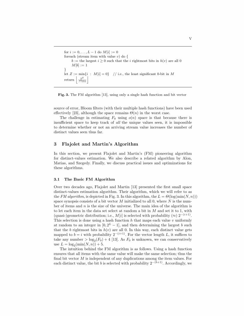
for i := 0, . . . , L − 1 do M [i] := 0foreach (stream item with value v) do

b := the largest i ≥ 0 such that the i rightmost bits in h(v) are all 0M [b] := 1

let Z := mini : M [i] = 0 // i.e., the least significant 0-bit in M

return⌊

2Z

.77351

⌋

Fig. 3. The FM algorithm [13], using only a single hash function and bit vector

source of error, Bloom filters (with their multiple hash functions) have been usedeffectively [23], although the space remains Θ(n) in the worst case.

The challenge in estimating F0 using o(n) space is that because there isinsufficient space to keep track of all the unique values seen, it is impossibleto determine whether or not an arriving stream value increases the number ofdistinct values seen thus far.

3 Flajolet and Martin’s Algorithm

In this section, we present Flajolet and Martin’s (FM) pioneering algorithmfor distinct-values estimation. We also describe a related algorithm by Alon,Matias, and Szegedy. Finally, we discuss practical issues and optimizations forthese algorithms.

3.1 The Basic FM Algorithm

Over two decades ago, Flajolet and Martin [13] presented the first small spacedistinct-values estimation algorithm. Their algorithm, which we will refer to asthe FM algorithm, is depicted in Fig. 3. In this algorithm, the L = Θ(log(min(N,n)))space synopsis consists of a bit vector M initialized to all 0, where N is the num-ber of items and n is the size of the universe. The main idea of the algorithm isto let each item in the data set select at random a bit in M and set it to 1, with(quasi-)geometric distribution; i.e., M [i] is selected with probability (≈) 2−(i+1).This selection is done using a hash function h that maps each value v uniformlyat random to an integer in [0, 2L − 1], and then determining the largest b suchthat the b rightmost bits in h(v) are all 0. In this way, each distinct value getsmapped to b = i with probability 2−(i+1). For the vector length L, it suffices totake any number > log2(F0) + 4 [13]. As F0 is unknown, we can conservativelyuse L = log2(min(N,n)) + 5.

The intuition behind the FM algorithm is as follows. Using a hash functionensures that all items with the same value will make the same selection; thus thefinal bit vector M is independent of any duplications among the item values. Foreach distinct value, the bit b is selected with probability 2−(b+1). Accordingly, we

VI

Item Hash Function 1 Hash Function 2 Hash Function 3value v b M [·] b M [·] b M [·]

15 1 00000010 1 00000010 0 0000000136 0 00000011 1 00000010 0 000000014 0 00000011 0 00000011 0 0000000129 0 00000011 2 00000111 1 000000119 3 00001011 0 00000111 0 0000001136 0 00001011 1 00000111 0 0000001114 1 00001011 0 00000111 1 000000114 0 00001011 0 00000111 0 00000011

Z = 2 Z = 3 Z = 2

Estimate F0 =⌊

2(2+3+2)/3

.77351

⌋

= 6

Fig. 4. Example run of the FM algorithm on a stream of 8 items, using three hashfunctions. Each M [·] is depicted as an L = 8 bit binary number, with M [0] being therightmost bit shown. The estimate, 6, matches the number of distinct values in thestream.

expect M [b] to be set if there are at least 2b+1 distinct values. Because bit Z − 1is set but not bit Z, there are likely greater than 2Z but fewer than 2Z+1 distinctvalues. Flajolet and Martin’s analysis shows that E[Z] ≈ log2(.77351 · F0), sothat 2Z/.77351 is a good choice in that range.

To reduce the variance in the estimator, Flajolet and Martin take the aver-age over tens of applications of this procedure (with different hash functions).Specifically, they take the average, Z, of the Z’s for different hash functions and

then compute⌊

2Z/.77351⌋

. An example is given in Fig. 4.

The error guarantee, space bound, and time bound are summarized in thefollowing theorem.

Theorem 1. [13] The FM algorithm with k (idealized) hash functions producesan estimator with standard error O(1/

√k), using k · L memory bits for the bit

vectors, for any L > log2(min(N,n))+4. For each item, the algorithm performsO(k) operations on L-bit memory words.

The space bound does not include the space for representing the hash functions.The time bound assumes that computing h and b are constant time operations.Sections 3.3 and 3.4 will present optimizations that significantly reduce both thespace for the bit vectors and the time per item, without increasing the standarderror.

3.2 The AMS Algorithm

Flajolet and Martin [13] analyze the error guarantees of their algorithm assumingthe use of an explicit family of hash functions with ideal random properties(namely, that h maps each value v uniformly at random to an integer in the

VII

Consider a universe U = 1, 2, . . . , n. Let d be the smallest integer so that 2d > n

Consider the members of U as elements of the finite field F = GF (2d),which are represented by binary vectors of length d

Let a and b be two random members of F , chosen uniformly and independentlyDefine h(v) := a · v + b, where the product and addition are computed in the field FR := 0foreach (stream item with value v) do

b := the largest i ≥ 0 such that the i rightmost bits in h(v) are all 0R := max(R, b)

return 2R

Fig. 5. The AMS algorithm [1], using only a single hash function

given range). Alon, Matias, and Szegedy [1] adapted the FM algorithm to use(more realistic) linear hash functions. Their algorithm, which we will call theAMS algorithm, produces an estimate with provable guarantees on the ratioerror. We discuss the AMS algorithm in this section.

First, note that in general, the final bit vector M returned by the FM algo-rithm in Section 3.1 consists of three parts, where the first part is all 0’s, thethird part is all 1’s, and the second part (called the fringe in [13]) is a mix of 0’sand 1’s that starts with the most significant 1 and ends with the least significant0. Let R (Z) be the position of the most (least) significant bit that is set to 1 (0,respectively). For example, for M [·] = 000101111, R = 5 and Z = 4. Whereasthe FM algorithm uses Z in its estimate, the AMS algorithm uses R. Namely,the estimate is 2R. Fig. 5 presents the AMS algorithm. Note that unlike theFM algorithm, the AMS algorithm does not maintain a bit vector but insteaddirectly keeps track of the most significant bit position set to 1.

The space bound and error guarantees for the AMS algorithm are summa-rized in the following theorem.

Theorem 2. [1] For every r > 2, the ratio error of the estimate returned bythe AMS algorithm is at most r with probability at least 1 − 2/r. The algorithmuses Θ(log n) memory bits.

Proof. Let b(v) be the value of b computed for h(v). By the construction of h(),we have that for every fixed v, h(v) is uniformly distributed over F . Thus theprobability that b(v) ≥ i is precisely 1/2i. Moreover, for every fixed distinct v1

and v2, the probability that b(v1) ≥ i and b(v2) ≥ i is precisely 1/22i.Fix an i. For each element v ∈ U that appears at least once in the stream,

let Wv,i be the indicator random variable whose value is 1 if and only if b(v) ≥ i.Let Zi =

∑

Wv,i, where v ranges over all the F0 elements v that appear inthe stream. By linearity of expectation and because the expectation of eachWv,i is 1/2i, the expectation E[Zi] of Zi is F0/2i. By pairwise independence,the variance of Zi is F0

12i (1 − 1

2i ) < F0/2i. Therefore, by Markov’s Inequality,

VIII

if 2i > rF0 then Pr[Zi > 0] < 1/r, since E[Zi] = F0/2i < 1/r. Similarly, byChebyshev’s Inequality, if r2i < F0 then Pr[Zi = 0] < 1/r, since Var[Zi] <F0/2i = E[Zi] and hence Pr[Zi = 0] ≤ Var[Zi]/(E[Zi]

2) < 1/E[Zi] = 2i/F0.Because the algorithm outputs F0 = 2R, where R is the maximum i for whichZi > 0, the two inequalities above show that the probability that the ratiobetween F0 and F0 is not between 1/r and r is smaller than 2/r, as needed.

As for the space bound, note that the algorithm uses d = O(log n) bitsrepresenting an irreducible polynomial needed in order to perform operationsin F , O(log n) bits representing a and b, and O(log log n) bits representing thecurrent maximum R value.

The probability of a given ratio error can be reduced by using multiple hashfunctions, at the cost of a linear increase in space and time.

Corollary 1. With k hash functions, the AMS algorithm uses O(k log n) mem-ory bits and, for each item, performs O(k) operations on O(log n)-bit memorywords.

The space bound includes the space for representing the hash functions. The timebound assumes that computing h(v) and b(v) are constant time operations.

3.3 Practical Issues

Although the AMS algorithm has stronger error guarantees than the FM al-gorithm, the FM algorithm is somewhat more accurate in practice, for a givensynopsis size [13]. In this section we argue why this is the case, and discuss otherimportant practical issues.

First, the most significant 1-bit (as is used in the AMS algorithm) can beset by a single outlier hashed value. For example, suppose a hashed value setsthe i’th bit whereas all other hashed values set bits ≤ i − 3, so that M [·] is ofthe form 0001001111. In such cases, it is clear from M that 2i is a significantoverestimate of F0: it is not supported by the other bits (in particular, both bitsi − 1 and i − 2 are 0’s not 1’s). On the other hand, the least significant 0-bit(as is used in the FM algorithm) is supported by all the bits to its right, whichmust be all 1’s. Thus FM is more robust against single outliers.

Second, although the AMS algorithm requires only ≈ log log n bits to repre-sent the current R, while the FM algorithm needs ≈ log n bits to represent thecurrent M [·], this space savings is insignificant compared to the O(log n) bits theAMS algorithm uses for the hash function computations. In practice, the sameclass of hash functions (i.e., h(v) = a · v + b) can be used in the FM algorithm,so that it too uses O(log n) bits per hash function.

Note that there are common scenarios where the space for the hash functionsis not as important as the space for the accumulated synopsis (i.e., R or M [·]).For example, in the distributed streams scenario (discussed in Section 6), anaccumulated synopsis is computed for each stream locally. In order to estimatethe total number of distinct values across all streams, the current accumulatedsynopses are collected. Thus the message size depends only on the accumulatedsynopsis size. Similarly, when distinct-values estimation techniques are used for

IX

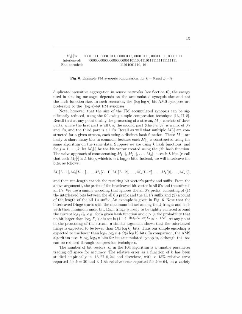
Mj [·]’s: 00001111, 00001011, 00000111, 00010111, 00011111, 00001111Interleaved: 000000000000000000000110110011101111111111111111

End-encoded: 11011001110, 16

Fig. 6. Example FM synopsis compression, for k = 6 and L = 8

duplicate-insensitive aggregation in sensor networks (see Section 6), the energyused in sending messages depends on the accumulated synopsis size and notthe hash function size. In such scenarios, the (log log n)-bit AMS synopses arepreferable to the (log n)-bit FM synopses.

Note, however, that the size of the FM accumulated synopsis can be sig-nificantly reduced, using the following simple compression technique [13, 27, 8].Recall that at any point during the processing of a stream, M [·] consists of threeparts, where the first part is all 0’s, the second part (the fringe) is a mix of 0’sand 1’s, and the third part is all 1’s. Recall as well that multiple M [·] are con-structed for a given stream, each using a distinct hash function. These M [·] arelikely to share many bits in common, because each M [·] is constructed using thesame algorithm on the same data. Suppose we are using k hash functions, andfor j = 1, . . . , k, let Mj [·] be the bit vector created using the jth hash function.The naive approach of concatenating M1[·], M2[·], . . . , Mk[·] uses k ·L bits (recallthat each Mj [·] is L bits), which is ≈ k log2 n bits. Instead, we will interleave thebits, as follows:

M1[L−1],M2[L−1], . . . ,Mk[L−1],M1[L−2], . . . ,Mk[L−2], . . . ,M1[0], . . . ,Mk[0],

and then run-length encode the resulting bit vector’s prefix and suffix. From theabove arguments, the prefix of the interleaved bit vector is all 0’s and the suffix isall 1’s. We use a simple encoding that ignores the all 0’s prefix, consisting of (1)the interleaved bits between the all 0’s prefix and the all 1’s suffix and (2) a countof the length of the all 1’s suffix. An example is given in Fig. 6. Note that theinterleaved fringe starts with the maximum bit set among the k fringes and endswith their minimum unset bit. Each fringe is likely to be tightly centered aroundthe current log2 F0, e.g., for a given hash function and c > 0, the probability thatno bit larger than log2 F0 +c is set is (1−2−(log2 F0+c))F0 ≈ e−1/2c

. At any pointin the processing of the stream, a similar argument shows that the interleavedfringe is expected to be fewer than O(k log k) bits. Thus our simple encoding isexpected to use fewer than log2 log2 n+O(k log k) bits. In comparison, the AMSalgorithm uses k log2 log2 n bits for its accumulated synopsis, although this toocan be reduced through compression techniques.

The number of bit vectors, k, in the FM algorithm is a tunable parametertrading off space for accuracy. The relative error as a function of k has beenstudied empirically in [13, 27, 8, 24] and elsewhere, with < 15% relative errorreported for k = 20 and < 10% relative error reported for k = 64, on a variety

X

for j := 1, . . . , k and i := 0, . . . , L − 1 do Mj [i] := 0foreach (stream item with value v) do

x := h(v) mod k // Note: k is a power of 2b := the largest i ≥ 0 such that the i rightmost bits in ⌊h(v)/k⌋ are all 0Mx[b] := 1

Z := 1

k

∑k

j=1mini : Mj [i] = 0

return⌊

k.77351

2Z⌋

Fig. 7. The PCSA algorithm [13]

of data sets. These studies show a strong diminishing return for increases ink. Theorem 1 shows that the standard error is O(1/

√k). Thus reducing the

standard error from 10% to 1% requires increasing k by a factor of 100! Ingeneral, to obtain a standard error at most ǫ we need k = Θ(1/ǫ2). Estan,Varghese and Fisk [12] present a number of techniques for further improving theconstants in the space vs. error trade-off, including using multi-resolution andadaptive bit vectors.

Both the FM and AMS algorithms use the largest i such that the i rightmostbits in h(v) are all 0, in order to create an exponential distribution onto an integerrange. A related, alternative approach by Cohen [7] is to (1) use a hash functionthat maps uniformly to the interval [0, 1], (2) maintain the minimum hashedvalue x seen thus far in the stream S (i.e., x = minv∈Sh(v)), and then (3)return 1

x − 1 as the estimate for F0. The intuition is that if there are F0 distinctvalues mapped uniformly at random to [0, 1], then we may expect them to dividethe interval into F0 + 1 relatively evenly-spaced subintervals, i.e., subintervalsof size 1

F0+1 . As [0, x] is the first such subinterval, x = 1F0+1 , and hence 1

x − 1is used as the estimate for F0. As with the FM and AMS algorithms, the errorguarantee can be improved by taking multiple hash functions and averaging.Empirically, this approach is not as accurate as the FM algorithm for a givensynopsis size [27].

3.4 Improving the Per-Item Processing Time

The FM algorithm as presented in Section 3.1 performs O(k) operations onmemory words of ≈ log2 n bits (recall Theorem 1) for each stream item. Thisis because a different hash function is used for each of the k bit vectors. Toreduce the processing time per item from O(k) to O(1), Flajolet and Martinpresent the following variant on their algorithm, called Probabilistic Countingwith Stochastic Averaging (PCSA).

In the PCSA algorithm (see Fig. 7), k bit vectors are used (for k a powerof 2) but only a single hash function h(). For each stream item with value v,the log2 k least significant bits of h(v) are used to select a bit vector. Then theremaining L − log2 k bits of h(v) are used to select a position within that bit

XI

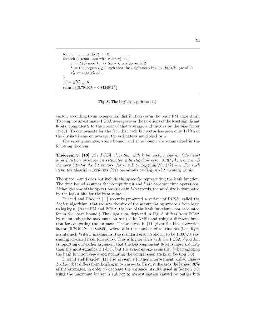
for j := 1, . . . , k do Rj := 0foreach (stream item with value v) do

x := h(v) mod k // Note: k is a power of 2b := the largest i ≥ 0 such that the i rightmost bits in ⌊h(v)/k⌋ are all 0Rx := max(Rx, b)

Z := 1

k

∑k

j=1Rj

return ⌊(0.79402k − 0.84249)2Z⌋

Fig. 8. The LogLog algorithm [11]

vector, according to an exponential distribution (as in the basic FM algorithm).To compute an estimate, PCSA averages over the positions of the least significant0-bits, computes 2 to the power of that average, and divides by the bias factor.77351. To compensate for the fact that each bit vector has seen only 1/k’th ofthe distinct items on average, the estimate is multiplied by k.

The error guarantee, space bound, and time bound are summarized in thefollowing theorem.

Theorem 3. [13] The PCSA algorithm with k bit vectors and an (idealized)hash function produces an estimator with standard error 0.78/

√k, using k · L

memory bits for the bit vectors, for any L > log2(min(N,n)/k) + 4. For eachitem, the algorithm performs O(1) operations on (log2 n)-bit memory words.

The space bound does not include the space for representing the hash function.The time bound assumes that computing h and b are constant time operations.Although some of the operations use only L-bit words, the word size is dominatedby the log2 n bits for the item value v.

Durand and Flajolet [11] recently presented a variant of PCSA, called theLogLog algorithm, that reduces the size of the accumulating synopsis from log nto log log n. (As in FM and PCSA, the size of the hash function is not accountedfor in the space bound.) The algorithm, depicted in Fig. 8, differs from PCSAby maintaining the maximum bit set (as in AMS) and using a different func-tion for computing the estimate. The analysis in [11] gives the bias correctionfactor (0.79402k − 0.84249), where k is the number of maximums (i.e., Rj ’s)

maintained. With k maximums, the standard error is shown to be 1.30/√

k (as-suming idealized hash functions). This is higher than with the PCSA algorithm(supporting our earlier argument that the least-significant 0-bit is more accuratethan the most-significant 1-bit), but the synopsis size is smaller (when ignoringthe hash function space and not using the compression tricks in Section 3.3).

Durand and Flajolet [11] also present a further improvement, called Super-LogLog, that differs from LogLog in two aspects. First, it discards the largest 30%of the estimates, in order to decrease the variance. As discussed in Section 3.3,using the maximum bit set is subject to overestimation caused by outlier bits

XII

being set. By discarding the largest estimates, these outliers are discarded. Notethat a different correction factor is needed in order to compensate for this ad-ditional source of bias [11]. Second, it represents each maximum Rj using onlyL = log2(log2(n/k) + 3) bits, and again corrects for the additional bias. Theerror guarantee, space bound, and time bound are summarized in the followingtheorem.

Theorem 4. [11] The Super-LogLog algorithm with k maximums and an (ide-alized) hash function produces an estimator with standard error 1.05/

√k, using

k ·L memory bits for the maximums, where L = ⌈log2⌈log2(min(N,n)/k) + 3⌉⌉.For each item, the algorithm performs O(1) operations on (log2 n)-bit memorywords.

The space bound does not include the space for representing the hash function.The time bound assumes that computing h and b are constant time operations.Although some of the operations use only L-bit words, the word size is dominatedby the log2 n bits for the stream value v. The standard error 1.05/

√k for Super-

LogLog is higher than the 0.78/√

k error for PCSA. Comparing the synopsissizes (ignoring the hash functions), super-LogLog uses a fixed ≈ k log2 log2(n/k)bits, whereas PCSA using the compression tricks of Section 3.3 uses an expected≈ log2 log2 n + O(k log k) bits.

4 (ǫ, δ)-Approximation Schemes

None of the algorithms presented thus far provides the strong guarantees of an(ǫ, δ)-approximation scheme. In this section, we present two such algorithms:the Coordinated Sampling algorithm of Gibbons and Tirthapura [17], and animprovement by Bar-Yossef et al. [2] that achieves near optimal space.

4.1 Coordinated Sampling

Gibbons and Tirthapura [17] gave the first (ǫ, δ)-approximation scheme for F0.Their algorithm, called Coordinated Sampling, is depicted in Fig. 9.

In the algorithm, there are k = Θ(log(1/δ)) instances of the same procedure,differing only in their use of different hash functions hj(). For each instance, thehash function is used to assign each potential stream value to a “level”, such thathalf the values are assigned to level 0, a quarter to level 1, etc. The algorithmmaintains a set of the ≈ τ distinct stream values that have the highest levelsamong those observed thus far. More specifically, it keeps track of the minimumlevel ℓj such that there are at most τ distinct stream values with level at leastℓj , as well as the set, Sj , of these stream values.

As in the AMS algorithm (Section 3.2), any uniform pairwise independenthash function can be used for hj(); for example, linear hash functions can beused. Let bj(v) be the value of b computed in the algorithm for hj(v). Followingthe argument in Section 3.2, we have that Prbj(v) = ℓ = 1

2ℓ+1 and Prbj(v) ≥ℓ = 1

2ℓ for ℓ = 0, . . . , log n− 1. Hence, Sj is always a uniform random sample of

XIII

for j := 1, . . . , k do ℓj := 0, Sj := ∅ foreach (stream item with value v) do

for j := 1, . . . , k do b := the largest i ≥ 0 such that the i rightmost bits in hj(v) are all 0if b ≥ ℓj and (v, b) 6∈ Sj do

Sj := Sj ∪ (v, b)// if Sj is too large, discard the level ℓj sample points from Sj

while |Sj | > τ do Sj := Sj − (v′, b′) : b′ = ℓjℓj := ℓj + 1

return medianj=1,...,k(|Sj | · 2

ℓj )

Fig. 9. The Coordinated Sampling algorithm [17]. The values of k and τ depend on thedesired ǫ and δ: k = 36 log

2(1/δ) and τ = 36/ǫ2, where the constant 36 is determined

by the worst case analysis and can be much smaller in practice.

the distinct stream values observed thus far, where each value is in the samplewith probability 2−ℓj . Thus, Coordinated Sampling uses |Sj | ·2ℓj as the estimatefor the number of distinct values in the stream. To ensure that the estimate iswithin ǫ with probability 1 − δ, it computes the median over Θ(log(1/δ)) suchestimates.

Each step of the algorithm within the “for” loop can be done in constant(expected) time by maintaining the appropriate data structures, assuming (as wehave for the previous algorithms) that computing hash functions and determiningb are constant time operations. For example, each Sj can be stored in a hashtable Tj of 2τ entries, where the pair (v, b) is the hash key. This enables bothtests for whether a given (v, b) is in Sj and insertions of a new (v, b) into Sj

to be done in constant expected time. We can enable constant time trackingof the size of Sj by maintaining an array of log n + 1 “level” counters, one perpossible level, which keep track of the number of pairs in Sj for each level. Wealso maintain a running count of the size of Sj . This counter is incremented by 1upon insertion into Sj and decremented by the corresponding level counter upondeleting all pairs in a level. In the latter case, in order to quickly delete fromSj all such pairs, we leave these deleted pairs in place, removing them lazily asthey are encountered in subsequent visits to Tj . (We need not explicitly markthem as deleted because subsequent visits see that their level numbers are toosmall and treat them as deleted.)

The error guarantee, space bound, and time bound are summarized in thefollowing theorem. The space bound includes the space for representing the hash

XIV

functions. The time bound assumes that computing hash functions and b areconstant expected time operations.

Theorem 5. [17] The Coordinated Sampling algorithm provides an (ǫ, δ)-approx-

imation scheme, using O( log n log(1/δ)ǫ2 ) memory bits. For each item, the algorithm

performs an expected O(log(1/δ)) operations on (log2 n)-bit memory words.

Proof. We have argued above about the time bound. The space bound is O(k ·τ)

memory words, i.e., O( log n log(1/δ)ǫ2 ) memory bits.

In what follows, we sketch the proof that Coordinated Sampling is indeedan (ǫ, δ)-approximation scheme. A difficulty in the proof is that the algorithmdecides when to stop changing levels based on the outcome of random trials, andhence may stop at an incorrect level, and make correspondingly bad estimates.We will argue that the probability of stopping at a “bad” level is small, and canbe accounted for in the desired error bound.

Accordingly, consider the jth instance of the algorithm. For ℓ ∈ 0.. log nand v ∈ 1..n, we define the random variables Xℓ,v such that Xℓ,v = 1 if v’s levelis at least ℓ and 0 otherwise. For the stream S, we define Xℓ =

∑

v∈S Xℓ,v forevery level ℓ. Note that after processing S, the value of ℓj is the lowest numberedlevel f such that Xf ≤ τ . The algorithm uses the estimate 2f · Xf .

For every level ℓ ∈ 0 . . . log n, we define Bℓ such that Bℓ = 1 if 2ℓXℓ 6∈[(1 − ǫ)F0, (1 + ǫ)F0] and 0 otherwise. Level ℓ is “bad” if Bl = 1, and “good”otherwise. Let Eℓ denote the event that the final value of ℓj is ℓ i.e., that fequals ℓ. The heart of the proof is to show the following:

PrGiven instance produces an estimate not in [(1 − ǫ)F0, (1 + ǫ)F0] <1

3(1)

Let P be the probability in equation 1. Let ℓ∗ denote the first level such thatE[Xℓ∗ ] ≤ 2

3τ . The instance produces an estimate not within the target range ifBf is true for the level f such that Ef is true. Thus,

P =

log n∑

i=0

PrEi ∧ Bi <

ℓ∗∑

i=0

PrBi +

log n∑

i=ℓ∗+1

PrEi (2)

The idea behind using the inequality to separate the Bi terms from the Ei

terms is that the lower levels (until ℓ∗) are likely to have good estimates and thealgorithm is unlikely to keep going beyond level ℓ∗.

As in the proof for the AMS algorithm (Theorem 2), we have that for ℓ =0, . . . , log n − 1,

E[Xℓ] =F0

2ℓ, (3)

and

var[Xℓ] <F0

2ℓ(4)

XV

We will now show that

ℓ∗∑

i=0

PrBi <6

ǫ2τ(5)

To see this, we first express PrBi in terms of equation 3: PrBi = Pr|Xi −F0

2i | ≥ ǫF0

2i . Then, from equation 4 and using Chebyshev’s inequality, we have

PrBi < 2i

F0ǫ2 . Hence,∑ℓ∗

i=0 PrBi <∑ℓ∗

i=02i

F0ǫ2 = 2ℓ∗+1

F0·ǫ2Now, because ℓ∗

is the first level such that F0

2ℓ∗ ≤ 23τ , we have that F0 > 2ℓ∗−1 · 2

3τ . Thus,∑ℓ∗

i=0 PrBi < 2ℓ∗+1

F0·ǫ2< 6

ǫ2τ , establishing equation 5.Next, we will show that

log n∑

i=ℓ∗+1

PrEi <6

τ(6)

To see this, we first observe that∑log n

i=ℓ∗+1 PrEi = PrXℓ∗ > τ, because the

Ei’s are mutually exclusive. Because E[Xℓ∗ ] < 23τ , we have PrXℓ∗ > τ <

PrXℓ∗ − E[Xℓ∗ ] > τ3. By Chebyshev’s inequality and equation 4, this latter

probability is less than 9τ2 · F0

2ℓ∗ . Plugging in the fact that 23τ > E[Xℓ∗ ] = F0

2ℓ∗ ,

we obtain∑log n

i=ℓ∗+1 PrEi < 9τ2 · 2τ

3 , establishing equation 6.Plugging into equation 2 the results from equations 5 and 6, and setting

τ = 36/ǫ2, we have P < 16 + ǫ2

6 < 13 . Thus, equation 1 is established.

Finally, the median fails to be an (ǫ, δ) estimator of F0 if at least k/2 instancesof the algorithm fail. By equation 1, we expect < k/3 to fail, and hence byChernoff bounds, the probability the algorithm fails is less than exp(−k/36).Setting k = 36 log(1/δ) makes this probability less than δ, completing the proofof the theorem.

4.2 Improving the Space Bound

Bar-Yossef et al. [2] showed how to adapt the Coordinated Sampling algorithm inorder to improve the space bound. Specifically, their algorithm, which we call theBJKST algorithm, stores the elements in Sj using less space, as follows. Instead ofstoring the pair (v, b), as in Coordinated Sampling, the BJKST algorithm storesg(v), for a suitably chosen hash function g(). Namely, g() is a (randomly chosen)uniform pairwise independent hash function that maps values from [0..n− 1] tothe range [0..R−1], where R = 3((log n+1)τ)2. Thus only O(log log n+log(1/ǫ))bits are needed to store g(v). The level b for v is represented implicitly by storingthe hashed values as a collection of balanced binary search trees, one tree foreach level.

The key observation is that for any given instance of the algorithm, g() isapplied to at most (log n + 1) · τ distinct values. Thus, the choice of R ensuresthat with probability at least 5/6, g() is injective on these values. If g() is indeedinjective, then using g() did not alter the basic progression of the instance. The

XVI

alternative occurs with probability at most 1/6. To compensate, the BJKSTalgorithm uses a larger τ , namely, τ = 576/ǫ2, such that the probability of a badestimate can be bounded by 1/6. Because 1

6 + 16 = 1

3 , a result akin to equation 1can be established. Finally, taking the median over k = 36 log(1/δ) instancesresults in an (ǫ, δ)-approximation.

The error guarantee, space bound, and time bound are summarized in thefollowing theorem. The space bound includes the space for representing the hashfunctions. The time bound assumes that computing hash functions and b areconstant expected time operations.

Theorem 6. [2] The BJKST algorithm provides an (ǫ, δ)-approximation scheme,using O(( 1

ǫ2 (log(1/ǫ) + log log n) + log n) log(1/δ)) memory bits. For each item,the algorithm performs O(log(1/δ)) operations on (log2 n)-bit words plus at most

O( log(1/δ)ǫ2 ) operations on (log2(1/ǫ) + log2 log2 n)-bit words.

5 Lower Bounds

This section presents five key lower bound results for distinct-values estimation.The first lower bound shows that observing (nearly) the entire stream is

essential for obtaining good estimation error guarantees for all input streams.

Theorem 7. [5] Consider any (possibly adaptive and randomized) estimator forthe number of distinct values F0 that examines at most r items in a stream ofN items. Then, for any γ > e−r, there exists a worst case input stream suchthat with probability at least γ, the ratio error of the estimate F0 output by the

estimator is at least√

N−r2r ln 1

γ .

Thus when r = o(N), the ratio error is non-constant with high probability. Evenwhen 1% of the input is examined, the ratio error is at least 5 with probability> 1/2.

The second lower bound shows that randomization is essential for obtaininglow estimation error guarantees for all input streams, if we hope to use sublin-ear space. For this lower bound, we also provide the proof, as a representativeexample of how such lower bounds are proved.

Theorem 8. [1] Any deterministic algorithm that outputs, given one pass througha data stream of N = n/2 elements of U = 1, 2, . . . , n, an estimate with atmost 10% relative error requires Ω(n) memory bits.

Proof. Let G be a family of t = 2Ω(n) subsets of U , each of cardinality n/4 sothat any two distinct members of G have at most n/8 elements in common. (Theexistence of such a G follows from standard results in coding theory, and canbe proved by a simple counting argument). Fix a deterministic algorithm thatapproximates F0. For every two members G1 and G2 of G let A(G1, G2) be thestream of length n/2 starting with the n/4 members of G1 (in a sorted order)and ending with the set of n/4 members of G2 (in a sorted order). When the

XVII

algorithm runs, given a stream of the form A(G1, G2), the memory configurationafter it reads the first n/4 elements of the stream depends only on G1. By thepigeonhole principle, if the memory has less than log2 t bits, then there are twodistinct sets G1 and G2 in G, so that the content of the memory after readingthe elements of G1 is equal to that content after reading the elements of G2. Thismeans that the algorithm must give the same final output to the two streamsA(G1, G1) and A(G2, G1). This, however, contradicts the assumption, becauseF0 = n/4 for A(G1, G1) and F0 ≥ 3n/8 for A(G2, G1). Therefore, the answer ofthe algorithm makes a relative error that exceeds 0.1 for at least one of thesetwo streams. It follows that the space used by the algorithm must be at leastlog2 t = Ω(n), completing the proof.

The third lower bound shows that approximation is essential for obtaininglow estimation error guarantees for all input streams, if we hope to use sublinearspace.

Theorem 9. [1] Any randomized algorithm that outputs, given one pass througha data stream of at most N = 2n items of U = 1, 2, . . . , n, a number Y suchthat Y = F0 with probability at least 1− δ, for some fixed δ < 1/2, requires Ω(n)memory bits.

The fourth lower bound shows that Ω(log n) memory bits are required forobtaining low estimation error.

Theorem 10. [1] Any randomized algorithm that outputs, given one pass througha data stream of items from U = 1, 2, . . . , n, an estimate with at most a 10%relative error with probability at least 3/4 must use at least Ω(log n) memorybits.

The final lower bound shows that Ω(1/ǫ2) memory bits are required in orderto obtain an (ǫ, δ)-approximation scheme (even for constant δ).

Theorem 11. [34] For any δ independent of n and any ǫ, any randomizedalgorithm that outputs, given one pass through a data stream of items from U =1, 2, . . . , n, an estimate with at most an ǫ relative error with probability at least1 − δ must use at least Ω(min(n, 1/ǫ2)) memory bits.

Thus we have an Ω(1/ǫ2 +log n) lower bound for obtaining arbitrary relativeerror for constant δ and, by the BJKST algorithm, a nearly matching upperbound of O(1/ǫ2(log(1/ǫ) + log log n) + log n).

6 Extensions

In this section, we consider distinct-values estimation in a variety of importantscenarios beyond the basic data stream set-up. In Sections 6.1–6.5, we focuson sampling, sliding windows, update streams, distributed streams, and sensornetworks (ODI), respectively, as summarized in Table 2. Finally, Section 6.6highlights three additional settings studied in the literature.

XVIII

Algorithm Cite & Sampling Sliding Update Distributed ODISection Distinct Windows Streams Streams

FM [13]; 3.1 no no no yes yesPCSA [13]; 3.4 no no no yes yes

FM with log2 space 6.2, 6.3 no yes yes yes noAMS [1]; 3.2 no no no yes yesCohen [7]; 3.3 no no no yes yesLogLog [11]; 3.4 no no no yes yes

Coordinated Sampling [17]; 4.1 yes no no yes yesBJKST [2]; 4.2 no no no yes yes

Distinct Sampling [16]; 6.1 yes no no yes yesRandomized Wave [18]; 6.2 yes yes no yes yes

l0 Sketch [9]; 6.2 no no yes yes noGanguly [14]; 6.3 yes no yes yes noCLKB [8]; 6.5 no no no yes yes

Table 2. Scenarios handled by the main algorithms discussed in this section

6.1 Sampling Distinct

In addition to providing an estimate of the number of distinct values in thestream, several algorithms provide a uniform sample of the distinct values in thestream. Such a sample can be used for a variety of sampling-based estimationprocedures, such as estimating the mean, the variance, and the quantiles over thedistinct values. Algorithms that retain only hashed values, such as FM, PCSA,AMS, Cohen, LogLog, BJKST, l0 Sketch (Section 6.2) and CLKB (Section 6.5),do not provide such samples. In some cases, such as Cohen, the algorithm canbe readily adapted to produce a uniform sample (with replacement): For eachinstance (i.e., each hash function) of the algorithm, maintain not just the currentminimum hashed value but also the original value associated with this minimumhashed value. As long as two different values do not hash to the same mini-mum value for a given hash function, each parallel instance produces one samplepoint. In contrast, Coordinated Sampling, Randomized Wave (Section 6.2) andGanguly’s algorithm (Section 6.3) all directly provide a uniform sample of thedistinct values.

Gibbons [16] extended the sampling goal to a multidimensional data settingthat arises in a class of common databases queries. Here, the goal is to extracta uniform sample of the distinct values in a primary dimension, as before, butinstead of retaining only the randomly selected values V , the algorithm retainsa “same-value” sample for each value in V . Specifically, for each v ∈ V , thealgorithm maintains a uniform random sample chosen from all the stream itemswith value v. A user-specified parameter t determines the size of each of thesesame-value samples; if there are fewer than t stream items with a particularvalue, the algorithm retains them all. The algorithm, called Distinct Sampling,is similar to Coordinated Sampling (Fig. 9) in having log n levels, maintaining allvalues whose levels are above a current threshhold, and incrementing the level

XIX

select count(distinct target-attr) select count(distinct o custkey)from Table from orderswhere P where o orderdate ≥ ’2006-01-01’

(a) (b)

Fig. 10. (a) Distinct Values Query template (b) Example query

threshhold whenever a space bound is reached. However, instead of retainingone (v, b) pair for the value v, it starts by retaining each of the first t itemswith value v in the primary dimension, as well as a count, nv, of the numberof items in the stream with value v (including the current item). Then, uponobserving any subsequent items with value v, it maintains a uniform same-valuesample for v by adding the new item to the sample with probability t/nv, makingroom by discarding a random item among the t items currently in the samplefor v. Fig. 10 gives an example of the type of SQL query that can be wellestimated by the Distinct Sampling algorithm, where target-attr in Fig. 10(a) isthe primary dimension and the predicate P is typically on one or more of theother dimensions, as in Fig. 10(b). The estimate is obtained by first applyingthe predicate to the same-value samples, in order to estimate what fraction ofthe values in V would be eliminated by the predicate, and then outputting theoverall query estimate based on the number of remaining values.

6.2 Sliding Windows

The sliding windows setting is motivated by the desire to estimate the numberof distinct values over only the most recent stream items. Specifically, we aregiven a window size W , and the problem is to estimate the number of distinctvalues over a sliding window of the W most recent items. The goal is to usespace that is logarithmic in W (linear in W would be trivial). Datar et al. [10]observed that the FM algorithm can be extended to solve the sliding windowsproblem, by keeping track of the stream position of the most recent item thatset each FM bit. Then, when estimating the number of distinct values withinthe current sliding window, only those FM bits whose associated positions arewithin the window are considered to be set. This increases the space needed forthe FM algorithm by a logarithmic factor.

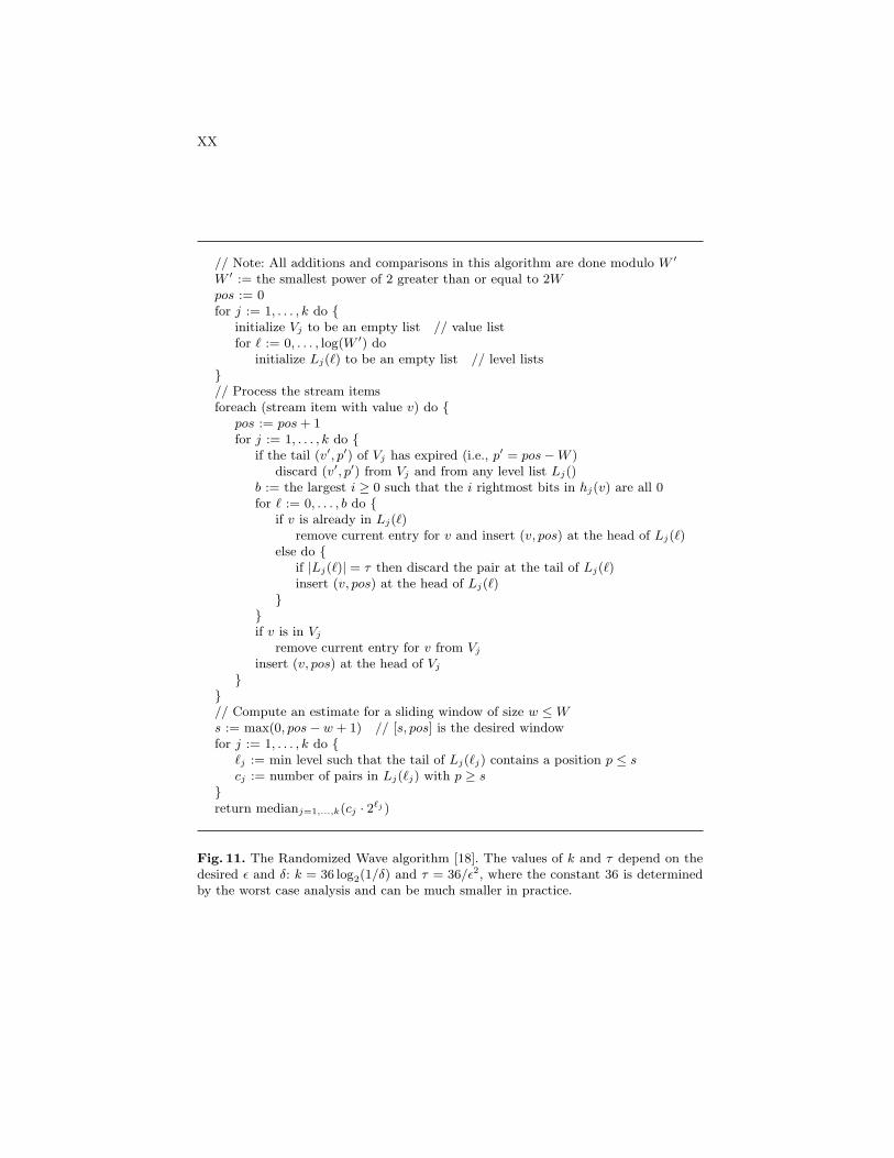
Gibbons and Tirthapura [18] developed an (ǫ, δ)-approximation scheme forthe sliding windows scenario. Their algorithm, called Randomized Wave, is de-picted in Fig. 11. In the algorithm, there are k = Θ(log(1/δ)) instances of thesame procedure, differing only in their use of different hash functions hj(). Anyuniform, pairwise independent hash function can be used for hj(). Let bj(v) bethe value of b computed in the algorithm for hj(v).

Whereas Coordinated Sampling maintained a single uniform sample of thedistinct values, Randomized Wave maintains ≈ log W uniform samples of the

XX

// Note: All additions and comparisons in this algorithm are done modulo W ′

W ′ := the smallest power of 2 greater than or equal to 2Wpos := 0for j := 1, . . . , k do

initialize Vj to be an empty list // value listfor ℓ := 0, . . . , log(W ′) do

initialize Lj(ℓ) to be an empty list // level lists// Process the stream itemsforeach (stream item with value v) do

pos := pos + 1for j := 1, . . . , k do

if the tail (v′, p′) of Vj has expired (i.e., p′ = pos − W )discard (v′, p′) from Vj and from any level list Lj()

b := the largest i ≥ 0 such that the i rightmost bits in hj(v) are all 0for ℓ := 0, . . . , b do

if v is already in Lj(ℓ)remove current entry for v and insert (v, pos) at the head of Lj(ℓ)

else do if |Lj(ℓ)| = τ then discard the pair at the tail of Lj(ℓ)insert (v, pos) at the head of Lj(ℓ)

if v is in Vj

remove current entry for v from Vj

insert (v, pos) at the head of Vj

// Compute an estimate for a sliding window of size w ≤ Ws := max(0, pos − w + 1) // [s, pos] is the desired windowfor j := 1, . . . , k do

ℓj := min level such that the tail of Lj(ℓj) contains a position p ≤ scj := number of pairs in Lj(ℓj) with p ≥ s

return medianj=1,...,k(cj · 2

ℓj )

Fig. 11. The Randomized Wave algorithm [18]. The values of k and τ depend on thedesired ǫ and δ: k = 36 log

2(1/δ) and τ = 36/ǫ2, where the constant 36 is determined

by the worst case analysis and can be much smaller in practice.

XXI

distinct values. Each of these “level” samples corresponds to a different samplingprobability, and retains only the τ = Θ(1/ǫ2) most recent distinct values sampledinto the associated level. (In the figure, Lj(ℓ) is the level sample for level ℓ ofinstance j.) An item with value v is selected into levels 0, . . . , bj(v), and stored asthe pair (v, pos), where pos is the stream position when v most recently occurred.

Each level sample Lj(ℓ) can be maintained as a doubly linked list. The al-gorithm also maintains a (doubly linked) list Vj of all the values in any of thelevel samples Lj(), together with the position of their most recent occurrences,ordered by position. This list enables fast discarding of items no longer withinthe sliding window. Finally, there is a hash table Hj (not shown in the figure)that holds triples (v, Vptr, Lptr), where v is a value in Vj , Vptr is a pointer tothe entry for v in Vj , and Lptr is a doubly linked list of pointers to each of theoccurrences of v in the level samples Lj(). These triples are stored in Hj hashedby their value v.

Consider an instance j. For each stream item, we first check the oldest valuev′ in Vj to see if its position is now outside of the window, and if so, we discard it.We use the triple in Hj(v

′) to locate all occurrences of v′ in the data structures;these occurrences are spliced out of their respective doubly linked lists. Second,we update the level samples Lj for each of the levels 0 . . . bj(v), where v is thevalue of the stream item. There are two cases. If v is not in the level sample, weinsert it, along with its position pos, at the head of the level sample. Otherwise,we perform a move-to-front: splicing out v’s current entry and inserting (v, pos)at the head of the level sample. In the former case, if inserting the new elementwould make the level sample exceed τ elements, we discard the oldest elementto make room. Finally, we insert (v, pos) at the head of Vj , and if v was alreadyin Vj , we splice out the old entry for v. Because the expected value of bj(v) isless than 2, v occurs in an expected constant number (in this case, 2) of levels.Thus, all of the above operations can be done in constant expected time.

Let (v′, p′) denote the pair at the tail of a level sample Lj(ℓ). Then Lj(ℓ)contains all the distinct values with stream positions in the interval [p′, pos]whose bj()’s are at least ℓ. Thus, similar to Coordinated Sampling, an estimateof the number of distinct values within a window can be obtained by taking thenumber of elements in Lj(ℓ) in this interval and multiplying by 2ℓ, the inverseof the sampling probability for the level.

The error guarantee, space bound, and time bound are summarized in thefollowing theorem. The space bound includes the space for representing the hashfunctions. The time bound assumes that computing hash functions and b areconstant expected time operations.

Theorem 12. [18] The Randomized Wave algorithm provides an (ǫ, δ)-approx-imation scheme for estimating the number of distinct values in any sliding win-

dow of size w ≤ W , using O( log n log W log(1/δ)ǫ2 ) memory bits, where the values

are in [0..n). For each item, the algorithm performs an expected O(log(1/δ))operations on max(log n, 2 + log W )-bit memory words.

Note that by setting W to be N , the length of the stream, the algorithmprovides an (ǫ, δ)-approximation scheme for all possible window sizes.

XXII

6.3 Update Streams

Another important scenario is where the stream contains both new items and thedeletion of previous items. Examples include estimating the current number ofdistinct network connections, phone connections or IP flows, where the streamcontains both the start and the end of each connection or flow. Most of thedistinct-values algorithms discussed thus far are not designed to handle deletions.For example, algorithms that retain only the maximum of some quantity, suchas AMS, Cohen and LogLog, or even the top few highest priority items, suchas Coordinated Sampling and BJKST, are unable to properly account for thedeletion of the current maximum or a high priority item. Similarly, once a biti is set in the FM algorithm, the subsequent deletion of an item mapped tobit i does not mean the bit can be unset: there are likely to have been otherun-deleted stream items that also mapped to bit i. In the case of FM, deletionscan be handled by replacing each bit with a running counter that is incrementedon insertions and decremented on deletions—at a cost of increasing the spaceneeded by a logarithmic factor.

Update streams generalize the insertion and deletion scenario by having eachstream item being a pair (v,∆), where ∆ > 0 specifies ∆ insertions of the valuev and ∆ < 0 specifies |∆| deletions of the value v. The resulting frequencyfv =

∑

(v,∆)∈S ∆ of value v is assumed to be nonnegative. The metric F0 is thenumber of distinct values v with fv > 0. The above variant of FM with coun-ters instead of bits readily handles update streams. Cormode et al. [9] devisedan (ǫ, δ)-approximation scheme, called l0 sketch, for distinct-values estimationover update streams. Unlike any of the approaches discussed thus far, the l0sketch algorithm uses properties of stable distributions, and requires floatingpoint arithmetic. The algorithm uses O( 1

ǫ2 log(1/δ)) floating point numbers andO( 1

ǫ2 log(1/δ)) floating point operations per stream item.Recently, Ganguly [14] devised two (ǫ, δ)-approximation schemes for up-

date streams. One uses O( 1ǫ2 (log n + log N) log N log(1/δ)) memory bits and

O(log(1/ǫ)· log(1/δ)) operations to process each stream update. The other usesa factor of (log(1/ǫ) + log(1/δ)) times more space but reduces the number ofoperations to only O(log(1/ǫ) + log(1/δ)). Both algorithms return a uniformsampling of the distinct values, as well as an estimate.

6.4 Distributed Streams

In a number of the motivating scenarios, the goal is to estimate the numberof distinct values over a collection of distributed streams. For example, in net-work monitoring, each router observes a stream of packets and the goal is toestimate the number of distinct “values” (e.g., destination IP addresses, source-destination pairs, requested urls, etc.) across all the streams. Formally, we havet ≥ 2 data streams, S1, S2, . . . , St, of items, where each item is from a universeof n possible values. Each stream Si is observed and processed by a party, Pi,independently of the other streams, in one pass and with limited working spacememory. The working space can be initialized (prior to observing any stream

XXIII

data) with data shared by all parties, so that, for example, all parties can usethe same random hash function(s). The goal is to estimate the number of distinctvalues in the multi-set arising from concatenating all t streams. For example, inthe t = 2 streams in Fig. 1, there are 15 distinct values in the two streamsaltogether.

In response to a request to produce an estimate, each party sends a message(containing its current synposis or some function of it) to a Referee, who outputsthe estimate based on these messages. Note that the parties do not communicatedirectly with one another, and the Referee does not directly observe any streamdata. We are primarily interested in minimizing: (1) the workspace used by eachparty, and (2) the time taken by a party to process a data item.

As shown in Table 2, each of the algorithms discussed in this chapter canbe readily adapted to handle the distributed streams setting. For example, theFM algorithm (Fig. 3) can be applied to each stream independently, using theexact same hash function across all streams, to generate a bit vector M [·] for eachstream. These bit vectors are sent to the Referee. Because the same hash functionwas used by all parties, the bit-wise OR of these t bit vectors yields exactlythe bit vector that would have been produced by running the FM algorithmon the concatenation of the t streams (or any other interleaving of the streamdata). Thus, the Referee computes this bit-wise OR, and then computes Z,the least significant 0-bit in the result. As in the original FM algorithm, wereduce the variance in the estimator by using k hash functions instead of just1, where all parties use the same k hash functions. The Referee computes theZ corresponding to each hash function, then computes the average, Z, of theseZ’s, and finally, outputs ⌊2Z/.77351⌋. The error guarantees of this distributedstreams algorithm match the error guarantees in Theorem 1 for the single-streamalgorithm. Moreover, the per-party space bound and the per-item time boundalso match the space and time bounds in Theorem 1.

Similarly, PCSA, FM with log2 space, AMS, Cohen, and LogLog can beadapted to the distributed streams setting in a straightforward manner, pre-serving the error guarantees, per-party space bounds, and per-item time boundsof the single-stream algorithm.

A bit less obvious, but still relatively straightforward, is adapting algorithmsthat use dynamic threshholds on what to keep and what to discard, where thethreshhold adjusts to the locally-observed data distribution. The key observationfor why these algorithms do not pose a problem is that we can match the errorguarantees of the single-stream algorithm by having the Referee use the strictestthreshhold among all the local threshholds. (Here, “strictest” means that thesmallest fraction of the data universe has its items kept.) Namely, if ℓ is thestrictest threshhold, the Referee “subsamples” the synopses from all the partiesby applying the threshhold ℓ to the synopses. This unifies all the synopses to thesame threshhold, and hence the Referee can safely combine these synopses andcompute an estimate.

Consider, for example, the Coordinated Sampling algorithm (Fig. 9). Eachparty sends its sets S1, . . . , Sk and levels ℓ1, . . . , ℓk to the Referee. For j =

XXIV

1, . . . , k, the Referee computes ℓ∗j , the maximum value of the ℓj ’s from all theparties. Then, for each j, the Referee subsamples each of the Sj from the tparties, by discarding from Sj all pairs (v′, b′) such that b′ < ℓ∗j . Next, for eachj, the Referee determines the union, S∗

j , of all the subsampled Sj ’s. Finally, the

Referee outputs the median over all j of |S∗

j |·2l∗j . The error guarantees, per-partyspace bound, and per-item time bound match those in Theorem 5 for the single-stream algorithm [17]. The error guarantees follow because (1) S∗

j contains allpairs (v, b) with b ≥ ℓ∗j across all t streams, and (2) the size of each S∗

j is at leastas big as the size of the Sj at a party with level ℓj = ℓ∗j (i.e., at a party with nosubsampling), and this latter size was already sufficient to get a good estimatein the single-stream setting.

6.5 Order- and Duplicate-Insensitive (ODI)

Another interesting setting for distinct-values estimation algorithms arises inrobust aggregation in wireless sensor networks. In sensor network aggregation,an aggregate function (e.g., count, sum, average) of the sensors’ readings isoften computed by having the wireless sensor nodes organize themselves intoa tree (with the base station as the root). The aggregate is computed bottom-upstarting at the leaves of the tree: each internal node in the tree combines itsown reading with the partial results from its children, and sends the result toits parent. For a sum, for example, the node’s reading is added to the sum ofits childrens’ respective partial sums. This conserves energy because each sensornode sends only one short message, in contrast to the naive approach of havingall readings forwarded hop-by-hop to the base station.

Aggregating along a tree, however, is not robust against message loss, whichis common in sensor networks, because each dropped message loses a subtree’sworth of readings. Thus, Considine et al. [8] and Nath et al. [24] proposed us-ing multi-path routing for more robust aggregation. In one scheme, the nodesorganize themselves into “rings” around the base station, where ring i consistsof all nodes that are i hops from the base station. As in the tree, aggregationis done bottom-up starting with the nodes in the ring furthest from the basestation (the “leaf” nodes). In contrast to the tree, however, when a node sendsits partial result, there is no designated parent. Instead, all nodes in the nextclosest ring that overhear the partial result incorporate it into their accumulat-ing partial results. Because of the added redundancy, the aggregation is highlyrobust to message loss, yet the energy consumption is similar to the (non-robust)tree because each sensor node sends only one short message.

On the other hand, because of the redundancy, partial results are accountedfor multiple times. Thus, the aggregation must be done in a duplicate-insensitivefashion. This is where distinct-values estimation algorithms come in. First, if thegoal is to count the number of distinct “values” (e.g., the number of distincttemperature readings), then a distinct-values estimation algorithm can be used,as long as the algorithm works for distributed streams and is insensitive to theduplication and observation re-ordering that arises in the scheme. An aggregation

XXV

algorithm with the combined properties of order- and duplicate-insensitivity iscalled ODI-correct [24]. Second, if the goal is to count the number of sensor nodeswhose readings satisfy a given boolean predicate (e.g., nodes with temperaturereadings below freezing), then again a distinct-values estimation algorithm canbe used, as follows. Each sensor node whose reading satisfies the predicate usesits unique sensor id as its “value”. Then the number of distinct values in thesensor network is precisely the desired count. Thus any distributed, ODI-correctdistinct-values estimation algorithm can be used.

As shown in Table 2, most of the algorithms discussed in this chapter are ODI-correct. For example, the FM algorithm (Fig. 3) is insensitive to both re-orderingand duplication: the bits that are set in an FM bit vector are independent of boththe order in which stream items are processed and any duplication of “partial-result” bit vectors (i.e., bit vectors corresponding to a subset of the streamitems). Moreover, Considine et al. [8] showed how the FM algorithm can beeffectively adapted to use only O(log log n) bit messages in this setting. Similarly,most of the other algorithms are ODI-correct, as can be proved formally usingthe approach described in [24].

6.6 Additional Settings

We conclude this chapter by briefly mentioning three additional important set-tings considered in the literature.

The first setting is distinct-values estimation when each value is unique. Thissetting occurs, for example, in distributed census taking over mobile objects(e.g., [31]). Here, there are a large number of objects, each with a unique id. Thegoal is to estimate how many objects there are despite the constant motion ofthe objects, while minimizing the communication. Clearly, any of the distributeddistinct-values estimation algorithms discussed in this chapter can be used. Note,however, that the setting enables a practical optimization: hash functions are notneeded to map values to bit positions or levels. Instead, independent coin tossescan be used at each object; the desired exponential distribution can be obtainedby flipping a fair coin until the first heads and counting the number of tailsobserved prior to the first head. (The unique id is not even used.) Obviatingthe need for hash functions eliminates their space and time overhead. Thus, forexample, only O(log log n)-bit synopses are needed for the AMS algorithm. Notethat hash functions were needed before to ensure that the multiple occurrencesof the same value all map to the same bit position or level; this feature is notneeded in the setting with unique values.

A second setting, studied by Bar-Yossef et al. [3] and Pavan and Tirtha-pura [28], seeks to estimate the number of distinct values where each stream itemis a range of integers. For example, in the 4-item stream [2, 5], [10, 12], [4, 8], [6, 7],there are 10 distinct values, namely, 2, 3, 4, 5, 6, 7, 8, 10, 11, and 12. Pavan

and Tirthapura present an (ǫ, δ)-approximation scheme that uses O( log n log(1/δ)ǫ2 )

memory bits, and performs an amortized O(log(1/δ) log(n/ǫ)) operations perstream item. Note that although a single stream item introduces up to n dis-

XXVI

tinct values into the stream, the space and time bounds have only a logarithmic(and not a linear) dependence on n.

Finally, a third important setting generalizes the distributed streams set-ting from just the union (concatenation) of the data streams to arbitrary set-expressions among the streams (including intersections and set differences). Inthis setting the number of distinct values corresponds to the cardinality of theresulting set. Ganguly et al. [15] showed how techniques for distinct values esti-mation can be generalized to handle this much richer setting.

References

1. Alon, N., Matias, Y., Szegedy, M.: The space complexity of approximating thefrequency moments. J. of Computer and System Sciences 58 (1999) 137–147

2. Bar-Yossef, Z., Jayram, T.S., Kumar, R., Sivakumar, D., Trevisan, L.: Count-ing distinct elements in a data stream. In: Proc. 6th International Workshop onRandomization and Approximation Techniques. (2002) 1–10

3. Bar-Yossef, Z., Kumar, R., Sivakumar, D.: Reductions in streaming algorithms,with an application to counting triangles in graphs. In: Proc. 13th ACM-SIAMSymposium on Discrete Algorithms (SODA). (2002)

4. Bunge, J., Fitzpatrick, M.: Estimating the number of species: A review. J. of theAmerican Statistical Association 88 (1993) 364–373

5. Charikar, M., Chaudhuri, S., Motwani, R., Narasayya, V.: Towards estimationerror guarantees for distinct values. In: Proc. 19th ACM Symp. on Principles ofDatabase Systems. (2000) 268–279

6. Chaudhuri, S., Motwani, R., Narasayya, V.: Random sampling for histogram con-struction: How much is enough? In: Proc. ACM SIGMOD International Conf. onManagement of Data. (1998) 436–447

7. Cohen, E.: Size-estimation framework with applications to transitive closure andreachability. J. of Computer and System Sciences 55 (1997) 441–453

8. Considine, J., Li, F., Kollios, G., Byers, J.: Approximate aggregation techniques forsensor databases. In: Proc. 20th International Conf. on Data Engineering. (2004)449–460

9. Cormode, G., Datar, M., Indyk, P., Muthukrishnan, S.: Comparing data streamsusing Hamming norms (how to zero in). In: Proc. 28th International Conf. on VeryLarge Data Bases. (2002) 335–345

10. Datar, M., Gionis, A., Indyk, P., Motwani, R.: Maintaining stream statistics oversliding windows. SIAM Journal on Computing 31 (2002) 1794–1813

11. Durand, M., Flajolet, P.: Loglog counting of large cardinalities. In: Proc. 11thEuropean Symp. on Algorithms. (2003) 605–617

12. Estan, C., Varghese, G., Fisk, M.: Bitmap algorithms for counting active flows onhigh speed links. In: Proc. 3rd ACM SIGCOMM Conf. on Internet Measurement.(2003) 153–166

13. Flajolet, P., Martin, G.N.: Probabilistic counting algorithms for data base appli-cations. J. of Computer and System Sciences 31 (1985) 182–209

14. Ganguly, S.: Counting distinct items over update streams. In: Proc. 16th Interna-tional Symp. on Algorithms and Computation. (2005) 505–514

15. Ganguly, S., Garofalakis, M., Rastogi, R.: Tracking set-expression cardinalitiesover continuous update streams. VLDB J. 13 (2004) 354–369

XXVII

16. Gibbons, P.B.: Distinct sampling for highly-accurate answers to distinct valuesqueries and event reports. In: Proc. 27th International Conf. on Very Large DataBases. (2001) 541–550

17. Gibbons, P.B., Tirthapura, S.: Estimating simple functions on the union of datastreams. In: Proc. 13th ACM Symp. on Parallel Algorithms and Architectures.(2001) 281–291

18. Gibbons, P.B., Tirthapura, S.: Distributed streams algorithms for sliding windows.In: Proc. 14th ACM Symp. on Parallel Algorithms and Architectures. (2002) 63–72

19. Haas, P.J., Naughton, J.F., Seshadri, S., Stokes, L.: Sampling-based estimation ofthe number of distinct values of an attribute. In: Proc. 21st International Conf. onVery Large Data Bases. (1995) 311–322

20. Haas, P.J., Stokes, L.: Estimating the number of classes in a finite population.J. of the American Statistical Association 93 (1998) 1475–1487

21. Hou, W.C., Ozsoyoglu, G., Taneja, B.K.: Statistical estimators for relational al-gebra expressions. In: Proc. 7th ACM Symp. on Principles of Database Systems.(1988) 276–287

22. Hou, W.C., Ozsoyoglu, G., Taneja, B.K.: Processing aggregate relational querieswith hard time constraints. In: Proc. ACM SIGMOD International Conf. on Man-agement of Data. (1989) 68–77

23. Kumar, A., Xu, J., Wang, J., Spatscheck, O., Li, L.: Space-code bloom filter forefficient per-flow traffic measurement. In: Proc. IEEE INFOCOM. (2004)

24. Nath, S., Gibbons, P.B., Seshan, S., Anderson, Z.: Synopsis diffusion for robust ag-gregation in sensor networks. In: Proc. 2nd ACM International Conf. on EmbeddedNetworked Sensor Systems. (2004) 250–262

25. Naughton, J.F., Seshadri, S.: On estimating the size of projections. In: Proc. 3rdInternational Conf. on Database Theory. (1990) 499–513

26. Olken, F.: Random Sampling from Databases. PhD thesis, Computer Science,U.C. Berkeley (1993)

27. Palmer, C.R., Gibbons, P.B., Faloutsos, C.: ANF: A fast and scalable tool for datamining in massive graphs. In: Proc. 8th ACM SIGKDD International Conf. onKnowledge Discovery and Data Mining. (2002) 81–90

28. Pavan, A., Tirthapura, S.: Range-efficient computation of F0 over massive datastreams. In: Proc. 21st IEEE International Conf. on Data Engineering. (2005)32–43

29. Poosala, V.: Histogram-based Estimation Techniques in Databases. PhD thesis,Univ. of Wisconsin-Madison (1997)

30. Poosala, V., Ioannidis, Y.E., Haas, P.J., Shekita, E.J.: Improved histograms forselectivity estimation of range predicates. In: Proc. ACM SIGMOD InternationalConf. on Management of Data. (1996) 294–305

31. Tao, Y., Kollios, G., Considine, J., Li, F., Papadias, D.: Spatio-temporal agge-gration using sketches. In: Proc. 20th International Conf. on Data Engineering.(2004) 214–225

32. Venkataraman, S., Song, D., Gibbons, P.B., Blum, A.: New streaming algorithmsfor high speed network monitoring and internet attacks detection. In: Proc. 12thISOC Network and Distributed Security Symp. (2005)

33. Whang, K.Y., Vander-Zanden, B.T., Taylor, H.M.: A linear-time probabilisticcounting algorithm for database applications. ACM Transactions on DatabaseSystems 15 (1990) 208–229

34. Woodruff, D.: Optimal space lower bounds for all frequency moments. In:Proc. 15th ACM-SIAM Symp. on Discrete Algorithms. (2004) 167–175