Distillation Theory

19

Draft - /home/ivarh/thesis/book/DistillationTheory_ch.fmVersion: 11 August 2000

Chapter 2

Distillation Theory

by

Ivar J. Halvorsen and Sigurd Skogestad

Norwegian University of Science and TechnologyDepartment of Chemical Engineering

7491 Trondheim, Norway

This is a revised version of an article acceptedfor publication in the Encyclopedia of SeparationScience by Academic Press Ltd. (submitted in1999). This article gives some of the basics ofdistillation theory and its purpose is to providebasic understanding and some tools for simple handcalculations of distillation columns. The methodspresented here can be used for simple estimates andto check more rigorous computations.

20


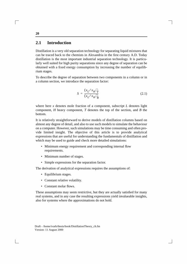
2.1 Introduction

Distillation is a very old separation technology for separating liquid mixtures thatcan be traced back to the chemists in Alexandria in the first century A.D. Todaydistillation is the most important industrial separation technology. It is particu-larly well suited for high purity separations since any degree of separation can beobtained with a fixed energy consumption by increasing the number of equilib-rium stages.

To describe the degree of separation between two components in a column or ina column section, we introduce the separation factor:

(2.1)

where herex denotes mole fraction of a component, subscriptL denotes lightcomponent,H heavy component,T denotes the top of the section, andB thebottom.

It is relatively straightforward to derive models of distillation columns based onalmost any degree of detail, and also to use such models to simulate the behaviouron a computer. However, such simulations may be time consuming and often pro-vide limited insight. The objective of this article is to provide analyticalexpressions that are useful for understanding the fundamentals of distillation andwhich may be used to guide and check more detailed simulations:

• Minimum energy requirement and corresponding internal flowrequirements.

• Minimum number of stages.

• Simple expressions for the separation factor.

The derivation of analytical expressions requires the assumptions of:

• Equilibrium stages.

• Constant relative volatility.

• Constant molar flows.

These assumptions may seem restrictive, but they are actually satisfied for manyreal systems, and in any case the resulting expressions yield invalueable insights,also for systems where the approximations do not hold.

SxL xH⁄( )

T

xL xH⁄( )B

------------------------=

2.2 Fundamentals 21


2.2 Fundamentals

2.2.1 The Equilibrium Stage Concept

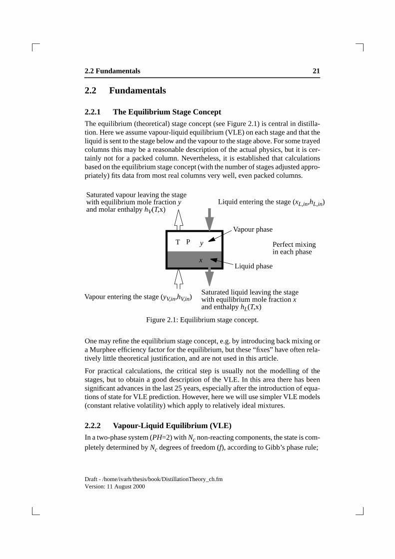
The equilibrium (theoretical) stage concept (see Figure 2.1) is central in distilla-tion. Here we assume vapour-liquid equilibrium (VLE) on each stage and that theliquid is sent to the stage below and the vapour to the stage above. For some trayedcolumns this may be a reasonable description of the actual physics, but it is cer-tainly not for a packed column. Nevertheless, it is established that calculationsbased on the equilibrium stage concept (with the number of stages adjusted appro-priately) fits data from most real columns very well, even packed columns.

Figure 2.1: Equilibrium stage concept.

One may refine the equilibrium stage concept, e.g. by introducing back mixing ora Murphee efficiency factor for the equilibrium, but these “fixes” have often rela-tively little theoretical justification, and are not used in this article.

For practical calculations, the critical step is usually not the modelling of thestages, but to obtain a good description of the VLE. In this area there has beensignificant advances in the last 25 years, especially after the introduction of equa-tions of state for VLE prediction. However, here we will use simpler VLE models(constant relative volatility) which apply to relatively ideal mixtures.

2.2.2 Vapour-Liquid Equilibrium (VLE)

In a two-phase system (PH=2) withNc non-reacting components, the state is com-pletely determined byNc degrees of freedom (f), according to Gibb’s phase rule;

y

x

PT

Vapour phase

Liquid phase

Saturated vapour leaving the stage

Saturated liquid leaving the stagewith equilibrium mole fractionx

with equilibrium mole fractiony

and enthalpyhL(T,x)

and molar enthalpyhV(T,x)Liquid entering the stage (xL,in,hL,in)

Vapour entering the stage (yV,in,hV,in)

Perfect mixingin each phase

22


(2.2)

If the pressure (P) andNc-1 liquid compositions or mole fractions (x) are used asdegrees of freedom, then the mole fractions (y) in the vapour phase and the tem-perature (T) are determined, provided that two phases are present. The generalVLE relation can then be written:

(2.3)

Here we have introduced the mole fractions x and y in the liquid an vapour phases

respectively, and we trivially have and

In idealmixtures, the vapour liquid equilibrium can be derived from Raoult’s lawwhich states that the partial pressurepi of a component (i) in the vapour phase is

proportional to the vapour pressure ( ) of the pure component (which is a func-

tion of temperature only: ) and the liquid mole fraction (xi):

(2.4)

For an ideas gas, according to Dalton’s law, the partial pressure of a componentis proportional to the mole fraction: , and since the total pressure

we derive:

(2.5)

The following empirical formula is frequently used for computing the pure com-ponent vapour pressure:

(2.6)

f Nc 2 P– H+=

y1 y2 … yNc 1– T, , , ,[ ] f P x1 x2 … xNc 1–, , , ,( )=

y T,[ ] f P x,( )=

xii 1=

n

∑ 1= yii 1=

n

∑ 1=

pio

pio

pio

T( )=

pi xi pio

T( )=

pi yiP=

P p1 p2 … pNc+ + + pi

i∑ xi pi

oT( )

i∑= = =

yi xi

pio

P------

xi pio

T( )

xi pio

T( )i

∑---------------------------= =

po

T( )ln ab

c T+------------ d T( )ln eT

f+ + +≈

2.2 Fundamentals 23


The coefficients are listed in component property data bases. The case withd=e=0is called the Antoine equation.

2.2.3 K-values and Relative Volatility

TheK-value for a componenti is defined as: . The K-value is some-

times called the equilibrium “constant”, but this is misleading as it dependsstrongly on temperature and pressure (or composition).

Therelative volatility between componentsi andj is defined as:

(2.7)

For ideal mixtures that satisfy Raoult’s law we have:

(2.8)

Here depends on temperature so the K-values will actually be constant

only close to the column ends where the temperature is relatively constant. On the

other hand the ratio is much less dependent on temperature which

makes the relative volatility very attractive for computations. For ideal mixtures,a geometric average of the relative volatilities for the highest and lowest temper-ature in the column usually gives sufficient accuracy in the computations:

.

We usually select a common reference componentr (usually the least volatile (or“heavy”) component), and define:

(2.9)

The VLE relationship (2.5) then becomes:

(2.10)

Ki yi xi⁄=

αij

yi xi⁄( )yj xj⁄( )

------------------Ki

K j------= =

αij

yi xi⁄( )yj xj⁄( )

------------------Ki

K j------

pio

T( )

pjo

T( )---------------= = =

pio

T( )

pio

T( ) pjo

T( )⁄

αij αij top, αij bottom,⋅=

αi αir pio

T( ) pro

T( )⁄= =

yi

αi xi

αi xii

∑-----------------=

24


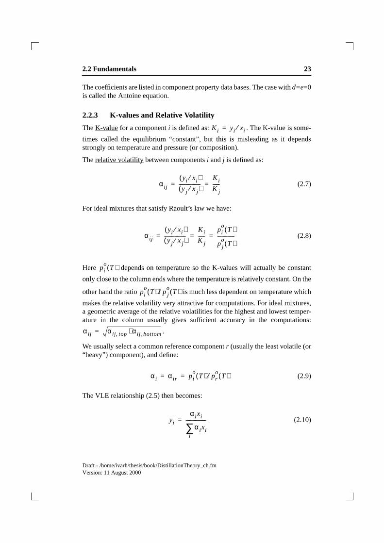
For a binary mixture we usually omit the component index for the light compo-nent, i.e. we writex=x1 (light component) andx2=1-x (heavy component). Thenthe VLE relationship becomes:

(2.11)

This equilibrium curve is illustrated in Figure 2.2:

Figure 2.2: VLE for ideal binary mixture:

The differencey-x determine the amount of separation that can be achieved on astage. Large relative volatilities implies large differences in boiling points andeasy separation. Close boiling points implies relative volatility closer to unity, asshown below quantitatively.

2.2.4 Estimating the Relative Volatility From Boiling Point Data

The Clapeyron equation relates the vapour pressure temperature dependency to

the specific heat of vaporization ( ) and volume change between liquid and

vapour phase ( ):

yαx

1 α 1–( )x+------------------------------=

Increasingα

Mole fraction

0 1

1

x

y

of light componentin liquid phase

Mole fractionof light componentin vapour phase

α=1

yαx

1 α 1–( )x+------------------------------=

Hvap∆

Vvap∆

2.2 Fundamentals 25


(2.12)

If we assume an ideal gas phase, and that the gas volume is much larger than the

liquid volume, then , and integration of Clapeyrons equationfrom temperatureTbi (boiling point at pressurePref) to temperatureT (at pressure

) gives, when is assumed constant:

(2.13)

This gives us the Antoine coefficients:

.

In most cases . For an ideal mixture that satisfies Raoult’s law we

have and we derive:

(2.14)

We see that the temperature dependency of the relative volatility arises from dif-

ferent specific heat of vaporization. For similar values ( ), the

expression simplifies to:

(2.15)

Here we may use the geometric average also for the heat of vaporization:

(2.16)

d po

T( )dT

------------------ Hvap∆ T( )

T Vvap

T( )∆----------------------------=

Vvap∆ RT P⁄≈

pio

Hivap∆

pio

ln∆Hi

vap

R---------------- 1

Tbi--------

Prefln+

∆Hivap

R----------------–

T-------------------------+≈

ai

∆Hivap

R---------------- 1

Tbi--------

Prefln+= bi,∆Hi

vap

R----------------–= ci, 0=

Pref 1 atm=

αij pio

T( ) pjo

T( )⁄=

αijln∆Hi

vap

R---------------- 1

Tbi--------

∆H jvap

R---------------- 1

Tbj--------–

∆H jvap ∆Hi

vap–

RT---------------------------------------+=

∆Hivap ∆H j

vap≈

αijln ≈ ∆Hvap

RTb------------------

β

Tbj Tbi–

Tb---------------------- where Tb TbiTbj=

∆Hvap ∆Hi

vapTbi( ) ∆H j

vapTbj( )⋅=

26


This results in a rough estimate of the relative volatility , based on the boiling

points only:

where (2.17)

If we do not know , a typical value can be used for many cases.

Example:For methanol (L) and n-propanol (H), we have

and and the heats of vaporization at their boiling points

are 35.3 kJ/mol and 41.8 kJ/mol respectively. Thus

and .

This gives and

which is a bit lower than the experimentalvalue.

2.2.5 Material Balance on a Distillation Stage

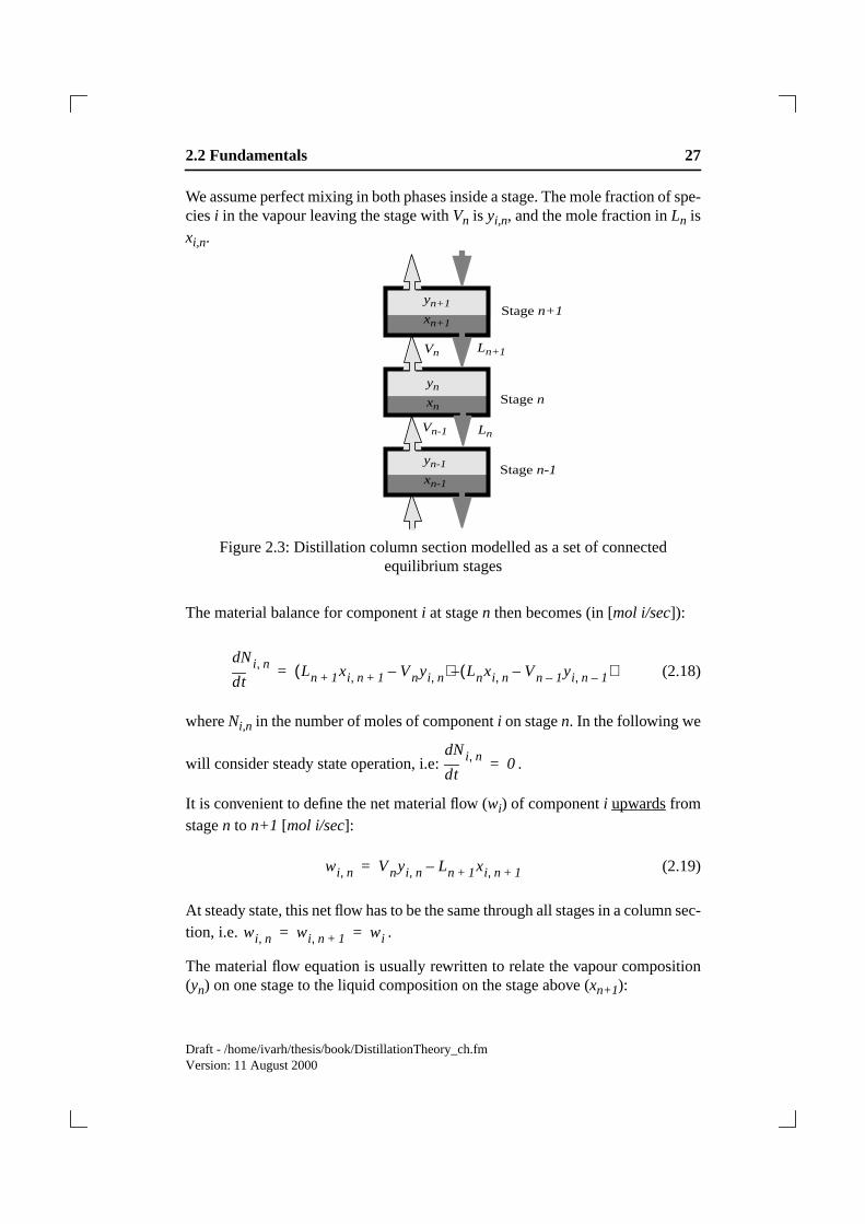
Based on the equilibrium stage concept, a distillation column section is modelledas shown in Figure 2.3: Note that we choose to number the stages starting fromthe bottom of the column. We denoteLn andVn as the total liquid- and vapourmolar flow rates leaving stagen (and entering stagesn-1 andn+1, respectively).

αij

αij eβ Tbj Tbi–( ) Tb⁄

≈ β ∆Hvap

RTB----------------=

∆Hvap β 13≈

TBL 337.8K=

TBH 370.4K=

TB 337.8 370.4⋅ 354K= = Hvap∆ 35.3 41.8⋅ 38.4= =

β ∆Hvap

RTB⁄ 38.4 8.83 354⋅( )⁄ 13.1= = =

α e13.1 32.6⋅ 354⁄ 3.34≈ ≈

2.2 Fundamentals 27


We assume perfect mixing in both phases inside a stage. The mole fraction of spe-ciesi in the vapour leaving the stage withVn is yi,n, and the mole fraction inLn isxi,n.

Figure 2.3: Distillation column section modelled as a set of connectedequilibrium stages

The material balance for componenti at stagen then becomes (in [mol i/sec]):

(2.18)

whereNi,n in the number of moles of componenti on stagen. In the following we

will consider steady state operation, i.e: .

It is convenient to define the net material flow (wi) of componenti upwards fromstagen to n+1 [mol i/sec]:

(2.19)

At steady state, this net flow has to be the same through all stages in a column sec-tion, i.e. .

The material flow equation is usually rewritten to relate the vapour composition(yn) on one stage to the liquid composition on the stage above (xn+1):

Ln+1

LnVn-1

Vn

yn

xn

yn+1

xn+1

yn-1

xn-1Stagen-1

Stagen

Stagen+1

td

dNi n, Ln 1+ xi n 1+, Vnyi n,–( ) Lnxi n, Vn 1– yi n 1–,–( )–=

td

dNi n, 0=

wi n, Vnyi n, Ln 1+ xi n 1+,–=

wi n, wi n 1+, wi= =

28


(2.20)

The resulting curve is known as theoperatingline. Combined with the VLE rela-tionship (equilibrium line) this enables us to compute all the stage compositionswhen we know the flows in the system. This is illustrated in Figure 2.4, and formsthe basis of the McCabe-Thiele approach.

Figure 2.4: Combining the VLE and the operating line to compute mole fractionsin a section of equilibrium stages.

2.2.6 Assumption about Constant Molar Flows

In a column section, we may very often use the assumption about constant molarflows. That is, we assume [mol/s] and [mol/

s]. This assumption is reasonable for ideal mixtures when the components havesimilar molar heat of vaporization. An important implication is that the operating

yi n,Ln 1+

Vn-------------xi n 1+,

1Vn------wi+=

xn-1

xn

xn

yn-1

yn

(2) Material balance

(1) VLE: y=f(x)

operating liney=(L/V)x+w/V

Use (1)

Use (2)

(1)

(2)

x

y

Ln Ln 1+ L= = Vn 1– Vn V= =

2.3 The Continuous Distillation Column 29


line is then a straight line for a given section, i.e .

This makes computations much simpler since the internal flows (L andV) do notdepend on compositions.

2.3 The Continuous Distillation Column

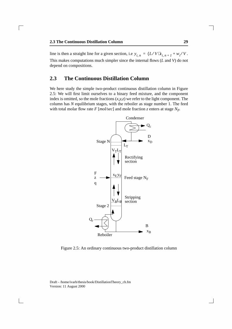
We here study the simple two-product continuous distillation column in Figure2.5: We will first limit ourselves to a binary feed mixture, and the componentindex is omitted, so the mole fractions (x,y,z) we refer to the light component. Thecolumn hasN equilibrium stages, with the reboiler as stage number 1. The feedwith total molar flow rateF [mol/sec] and mole fractionz enters at stageNF.

Figure 2.5: An ordinary continuous two-product distillation column

yi n, L V⁄( )xi n 1+, wi V⁄+=

Fzq

D

B

xD

xB

Qr

Qc

Rectifyingsection

Strippingsection

xF,yF

Condenser

Reboiler

LT

Stage 2

VTLT

Stage N

Feed stage NF

VBLB

30


The section above the feed stage is denoted the rectifying section, or just the topsection, and the most volatile component is enriched upwards towards the distil-late product outlet (D). The stripping section, or the bottom section, is below thefeed, in which the least volatile component is enriched towards the bottoms prod-uct outlet (B). (The least volatile component is “stripped” out.) Heat is suppliedin the reboiler and removed in the condenser, and we do not consider any heat lossalong the column.

The feed liquid fractionq describes the change in liquid and vapour flow rates atthe feed stage:

(2.21)

The liquid fraction is related to the feed enthalpy (hF) as follows:

(2.22)

When we assume constant molar flows in each section, we get the following rela-tionships for the flows:

(2.23)

2.3.1 Degrees of Freedom in Operation of a Distillation Column

With a given feed (F,z andq), and column pressure (P), we have only 2 degreesof freedom in operation of the two-product column in Figure 2.5, independent ofthe number of components in the feed. This may be a bit confusing if we thinkabout degrees of freedom as in Gibb’s phase rule, but in this context Gibb’s ruledoes not apply since it relates the thermodynamic degrees of freedom inside a sin-gle equilibrium stage.

LF∆ qF=

VF∆ 1 q–( )F=

qhV sat, hF–

Hvap∆

---------------------------

1> Subcooled liquid

1= Saturated liquid

0 q 1< < Liquid and vapour

0= Saturated vapour

0< Superheated vapour

= =

VT VB 1 q–( )F+=

LB LT qF+=

D VT LT–=

B LB VB–=



This implies that if we know, for example, the reflux (LT) and vapour (VB) flowrate into the column, all states on all stages and in both products are completelydetermined.

2.3.2 External and Internal Flows

The overall mass balance and component mass balance is given by:

(2.24)

Herez is the mole fraction of light component in the feed, andxD andxB are theproduct compositions. For sharp splits withxD≈ 1 andxB ≈ 0 we then have thatD=zF. In words, we must adjust the product splitD/F such that the distillate flowequals the amount of light component in the feed. Any deviation from this valuewill result in large changes in product composition. This is a very importantinsight for practical operation.

Example:Consider a column with z=0.5, xD=0.99, xB=0.01 (all these refer

to the mole fraction of light component) and D/F = B/F = 0.5. To simplifythe discussion set F=1 [mol/sec]. Now consider a 20% increase in the dis-tillate D from 0.50 to 0.6 [mol/sec]. This will have a drastic effect oncomposition. Since the total amount of light component available in thefeed is z = 0.5 [mol/sec], at least 0.1 [mol/sec] of the distillate must now beheavy component, so the amount mole fraction of light component in thedistillate is now at its best 0.5/0.6 = 0.833. In other words, the amount ofheavy component in the distillate will increase at least by a factor of 16.7(from 1% to 16.7%).

Thus, we generally have that a change inexternal flows(D/F andB/F) has a largeeffect on composition, at least for sharp splits, because any significant deviationin D/F from z implies large changes in composition. On the other hand, the effectof changes in theinternal flows (L andV) are much smaller.

2.3.3 McCabe-Thiele Diagram (Constant Molar Flows, but anyVLE)

The McCabe-Thiele diagram wherey is plotted as a functionx along the columnprovides an insightful graphical solution to the combined mass balance (“opera-tion line”) and VLE (“equilibrium line”) equations. It is mainly used for binarymixtures. It is often used to find the number of theoretical stages for mixtures withconstant molar flows. The equilibrium relationship (y as a function

of x at the stages) may be nonideal. With constant molar flow, L and V are con-

F D B+=

Fz DxD BxB+=

yn f xn( )=

32


stant within each section and the operating lines (y as a function ofx between thestages) are straight. In the top section the net transport of light component

. Inserted into the material balance equation (2.20) we obtain the oper-

ating line for the top section, and we have a similar expression for the bottomsection:

(2.25)

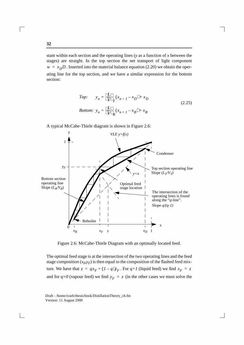
A typical McCabe-Thiele diagram is shown in Figure 2.6:

Figure 2.6: McCabe-Thiele Diagram with an optimally located feed.

The optimal feed stage is at the intersection of the two operating lines and the feedstage composition (xF,yF) is then equal to the composition of the flashed feed mix-

ture. We have that . Forq=1 (liquid feed) we find

and forq=0 (vapour feed) we find (in the other cases we must solve the

w xDD=

Top: ynLV----

T

xn 1+ xD–( ) xD+=

Bottom: ynLV----

B

xn 1+ xB–( ) xB+=

01

1

xF

y

y=x

xDxB

yF

x

Top section operating line

VLE y=f(x)

Bottom sectionOptimal feed

Reboiler

Condenser

z

The intersection of the

Slope (LT/VT)

operating lineSlope (LB/VB)

Slope q/(q-1)along the “q-line”.

stage location

operating lines is found

z qxF 1 q–( )yF+= xF z=

yF z=



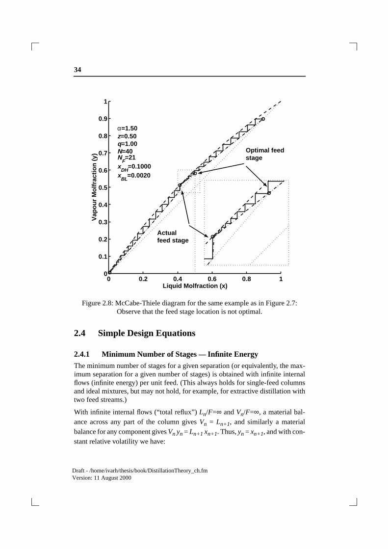
equation together with the VLE). The pinch, which occurs at one side of the feedstage if the feed is not optimally located, is easily understood from the McCabe-Thiele diagram as shown in Figure 2.8:

2.3.4 Typical Column Profiles— Pinch

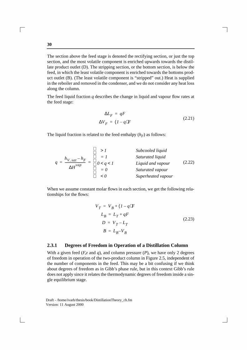
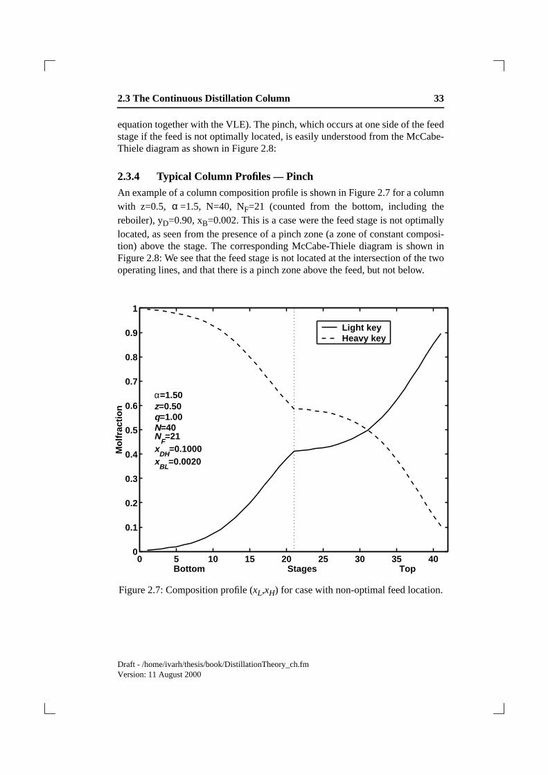
An example of a column composition profile is shown in Figure 2.7 for a columnwith z=0.5, =1.5, N=40, NF=21 (counted from the bottom, including thereboiler), yD=0.90, xB=0.002. This is a case were the feed stage is not optimallylocated, as seen from the presence of a pinch zone (a zone of constant composi-tion) above the stage. The corresponding McCabe-Thiele diagram is shown inFigure 2.8: We see that the feed stage is not located at the intersection of the twooperating lines, and that there is a pinch zone above the feed, but not below.

Figure 2.7: Composition profile (xL,xH) for case with non-optimal feed location.

α

0 5 10 15 20 25 30 35 400

0.1

0.2

0.3

0.4

0.5

0.6

0.7

0.8

0.9

1

Bottom Stages Top

Mol

frac

tion

α=1.50z=0.50q=1.00N=40N

F=21

xDH

=0.1000x

BL=0.0020

Light keyHeavy key

34


Figure 2.8: McCabe-Thiele diagram for the same example as in Figure 2.7:Observe that the feed stage location is not optimal.

2.4 Simple Design Equations

2.4.1 Minimum Number of Stages— Infinite Energy

The minimum number of stages for a given separation (or equivalently, the max-imum separation for a given number of stages) is obtained with infinite internalflows (infinite energy) per unit feed. (This always holds for single-feed columnsand ideal mixtures, but may not hold, for example, for extractive distillation withtwo feed streams.)

With infinite internal flows (“total reflux”)Ln/F=∞ andVn/F=∞, a material bal-ance across any part of the column givesVn = Ln+1, and similarly a materialbalance for any component givesVn yn = Ln+1 xn+1. Thus,yn = xn+1, and with con-stant relative volatility we have:

0 0.2 0.4 0.6 0.8 10

0.1

0.2

0.3

0.4

0.5

0.6

0.7

0.8

0.9

1V

apou

r M

olfr

actio

n (y

)

Liquid Molfraction (x)

α=1.50z=0.50q=1.00N=40N

F=21

xDH

=0.1000x

BL=0.0020

Optimal feedstage

Actualfeed stage

2.4 Simple Design Equations 35


(2.26)

For a column or column section withN stages, repeated use of this relation givesdirectly Fenske’s formula for the overall separation factor:

(2.27)

For a column with a given separation, this yields Fenske’s formula for the mini-mum number of stages:

(2.28)

These Fenske expressions do not assume constant molar flows and apply to theseparation between any two components with constant relative volatility. Notethat although a high-purity separation (largeS) requires a larger number of stages,the increase is only proportional to the logarithm of separation factor. For exam-ple, increasing the purity level in a product by a factor of 10 (e.g. by reducingxH,D

from 0.01 to 0.001) increasesNmin by about a factor of .

A common rule of thumb is to select the actual number of stages (or

even larger).

2.4.2 Minimum Energy Usage— Infinite Number of Stages

For a given separation, an increase in the number of stages will yield a reductionin the reflux (or equivalently in the boilup). However, as the number of stagesapproach infinity, a pinch zone develops somewhere in the column, and the refluxcannot be reduced further. For a binary separation the pinch usually occurs at thefeed stage (where the material balance line and the equilibrium line will meet),and we can easily derive an expression for the minimum reflux with . Fora saturatedliquid feed (q=1) (King’s formula):

(2.29)

αyL n,yH n,-----------

xL n,xH n,-----------⁄

xL n 1+,xH n 1+,-------------------

xL n,xH n,-----------⁄= =

SxL

xH------

T

xL

xH------

B

⁄ αN= =

NminSlnαln

---------=

10ln 2.3=

N 2Nmin=

N ∞=

LTmin

rL D, αrH D,–

α 1–----------------------------------F=

36


where is the recovery fraction of light component, and

of heavy component, both in the distillate. The value depends relatively weaklyon the product purity, and for sharp separations (where and

), we haveLmin= F/(α - 1). Actually, equation (2.29) applies without

stipulating constant molar flows or constantα, but thenLmin is the liquid flowentering the feed stage from above, andα is the relative volatility at feed condi-tions. A similar expression, but in terms of entering the feed stage from

below, applies for a saturatedvapour feed(q=0) (King’s formula):

(2.30)

For sharp separations we get =F/(α - 1). In summary, for a binary mixture

with constant molar flows and constant relative volatility, the minimum boilup forsharp separations is:

(2.31)

Note that minimum boilup is independent of the product purity for sharp separa-tions. From this we establish one of the key properties of distillation:We canachieve any product purity(even “infinite separation factor”)with a constantfinite energy(as long as it is higher thanthe minimum) by increasing the numberof stages.

Obviously, this statement does not apply to azeotropic mixtures, for whichα = 1for some composition, (but we can get arbitrary close to the azeotropic composi-tion, and useful results may be obtained in some cases by treating the azeotropeas a pseudo-component and usingα for this pseudo-separation).

2.4.3 Finite Number of Stages and Finite Reflux

Fenske’s formulaS= αΝ applies to infinite reflux (infinite energy). To extend thisexpression to real columns with finite reflux we will assume constant molar flowsand consider below three approaches:

1. Assume constant K-values and derive the Kremser formulas (exact close tothe column end for a high-purity separation).

r L D, xDD z⁄ F= rH D,

r L D, 1=

rH D, 0=

VBmin

VBmin

rH B, αr L B,–

α 1–---------------------------------F=

VBmin

Feed liquid, q=1: VBmin1

α 1–------------F D+=

Feed vapour, q=0: VBmin1

α 1–------------F=



2. Assume constant relative volatility and derive the following extended Fen-ske formula (approximate formula for case with optimal feed stagelocation):

(2.32)

HereNT is the number of stages in the top section andNB in the bottomsection.

3. Assume constant relative volatility and derive exact expressions. The mostused are the Underwood formulas which are particularly useful for com-puting the minimum reflux (with infinite stages).

2.4.4 Constant K-values— Kremser Formulas

For high-purity separations most of the stages are located in the “corner” parts ofthe McCabe-Thiele diagram where we according to Henry’s law may approxi-mate the VLE-relationship, even for nonideal mixtures, by straight lines;

Bottom of column: yL = HLxL (light component;xL→ 0)

Top of column: yH = HH xH (heavy component;xH → 0)

whereH is Henry’s constant. (For the case of constant relative volatility, Henry’sconstant in the bottom is and in the top is ). Thus, with con-

stant molar flows, both the equilibrium and mass-balance relationships are linear,and the resulting difference equations are easily solved analytically. For example,at the bottom of the column we derive for the light component:

(2.33)

where is the stripping factor. Repeated use of this equation

gives the Kremser formula for stageNB from the bottom (the reboiler would herebe stage zero):

(2.34)

(assumes we are in the region where s is constant, i.e. ).

S αN LT VT⁄( )NT

LB VB⁄( )NB

-----------------------------≈

HL α= HH 1 α⁄=

xL n 1+, VB LB⁄( )HLxL n, B LB⁄( )xL B,+=

sxL n, 1 VB– LB⁄( )xL B,+=

s VB LB⁄( )HL 1>=

xL NB, sNBxL B, 1 1 VB– LB⁄( ) 1 s N– B–( ) s 1–( )⁄+[ ]=

xL 0≈

38


At the top of the column we have for the heavy component:

(2.35)

where is the absorbtion factor. The corresponding

Kremser formula for the heavy component in the vapour phase at stageNT

counted from the top of the column (the accumulator is stage zero) is then:

(2.36)

(assumes we are in the region where a is constant, i.e. ).

For hand calculations one may use the McCabe-Thiele diagram for the interme-diate composition region, and the Kremser formulas at the column ends where theuse of the McCabe-Thiele diagram is inaccurate.

Example.We consider a column with N=40, NF=21, =1.5, zL=0.5, F=1,D=0.5, VB=3.2063. The feed is saturated liquid and exact calculations givethe product compositions xH,D= xL,B=0.01.We now want to have a bottom product with only 1 ppm heavy product, i.e.xL,B = 1.e-6. We can use the Kremser formulas to easily estimate the addi-tional stages needed when we have the same energy usage, VB=3.2063.(Note that with the increased purity in the bottom we actually get B=0.4949and LB=3.7012). At the bottom of the column and the

stripping factor is .

With xL,B=1.e-6 (new purity) and (old purity) we find by

solving the Kremser equation (2.34) with respect to NB that NB=33.94, andwe conclude that we need about 34 additional stages in the bottom (this isnot quite enough since the operating line is slightly moved and thus affectsthe rest of the column; using 36 rather 34 additional stages compensatesfor this).

The above Kremser formulas are valid at the column ends, but the linear approx-imation resulting from the Henry’s law approximation lies above the real VLEcurve (is optimistic), and thus gives too few stages in the middle of the column.However, if the there is no pinch at the feed stage (i.e. the feed is optimallylocated), then most of the stages in the column will be located at the columns endswhere the above Kremser formulas apply.

yH n 1–, LT VT⁄( ) 1 HH⁄( )yH n, D VT⁄( )xH D,+=

ayH n, 1 LT VT⁄–( )xH D,+=

a LT VT⁄( ) HH⁄ 1>=

yH NT, aNTxH D, 1 1 LT– VT⁄( ) 1 a N– T–( ) a 1–( )⁄+[ ]=

xH 0≈

α

HL α 1.5= =

s VB LB⁄( )HL 3.2063 3.712⁄( )1.5 1.2994= = =

xL NB, 0.01=



2.4.5 Approximate Formula with Constant Relative Volatility

We will now use the Kremser formulas to derive an approximation for the sepa-ration factor S. First note that for cases with high-purity products we have

That is, the separation factor is the inverse of the product of

the key component product impurities.

We now assume that the feed stage is optimally located such that the compositionat the feed stage is the same as that in the feed, i.e. and

Assuming constant relative volatility and using ,

, and (including

total reboiler) then gives:

(2.37)

where (2.38)

We know that S predicted by this expression is somewhat too large because of thelinearized VLE. However, we may correct it such that it satisfies the exact rela-

tionship at infinite reflux (where and c=1) by

dropping the factor (which as expected is always larger than 1). At

finite reflux, there are even more stages in the feed region and the formula willfurther oversestimate the value of S. However, since c > 1 at finite reflux, we maypartly counteract this by settingc=1. Thus, we delete the term c and arrive at thefinal extended Fenske formula, where the main assumptions are that we have con-stant relative volatility, constant molar flows, and that there is no pinch zonearound the feed (i.e. the feed is optimally located):

(2.39)

where .

S 1 xL B, xH D,( )⁄≈

yH NT, yH F,=

xL NB, xL F,= HL α=

HB 1 α⁄= α yLF xLF⁄( ) yHF xHF⁄( )⁄= N NT NB 1+ +=

S αNLT VT⁄( )NT

LB VB⁄( )NB----------------------------- c

xHFyLF( )------------------------≈

c 1 1VB

LB-------–

1 s NB––( )

s 1–( )-------------------------+ 1 1

LT

VT-------–

1 a NT––( )

a 1–( )-------------------------+=

S αN= LB VB⁄ VT LT⁄ 1= =

1 xHFyLF( )⁄

S αNLT VT⁄( )NT

LB VB⁄( )NB-----------------------------≈

N NT NB 1+ +=

40


Together with the material balance, , this approximate for-

mula can be used for estimating the number of stages for column design (insteadof e.g. the Gilliand plots), and also for estimating the effect of changes of internalflows during column operation. However, its main value is the insight it provides:

1. We see that the best way to increase the separationS is to increase thenumber of stages.

2. During operation whereN is fixed, the formula provides us with the impor-tant insight that the separation factorS is increased by increasing theinternalflowsL andV, thereby makingL/V closer to 1. However, the effectof increasing the internal flows (energy) is limited since the maximum sep-

aration with infinite flows is .

3. We see that the separation factorS depends mainly on the internal flows(energy usage) and only weakly on the splitD/F. This means that if wechangeD/F thenS will remain approximately constant (Shinskey’s rule),that is, we will get a shift in impurity from one product to the other suchthat the product of the impurities remains constant. This insight is veryuseful.

Example.Consider a column with (1% heavy in top) and

(1% light in bottom). The separation factor is then approxi-

mately Assume we slightlyincrease D from 0.50 to 0.51. If we assume constant separation factor(Shinskey’s rule), then we find that changes from 0.01 to 0.0236

(heavy impurity in the top product increases by a factor 2.4), whereas and changes from 0.01 to 0.0042 (light impurity in the bottom product

decreases by a factor 2.4). Exact calculations with column data: N=40,NF=21, =1.5, zL=0.5, F=1, D=0.5, LT/F=3.206, give that

changes from 0.01 to 0.0241 and changes from 0.01 to 0.0046 (sep-

aration factor changes from S=9801 to 8706). Thus, Shinskey’s rule givesvery accurate predictions.

However, the simple extended Fenske formula also has shortcomings. First, it issomewhat misleading since it suggests that the separation may always beimproved by transferring stages from the bottom to the top section if

. This is not generally true (and is not really “allowed” as it

violates the assumption of optimal feed location). Second, although the formula

FzF DxD BxB+=

S αN=

xD H, 0.01=

xB L, 0.01=

S 0.99 0.99 0.01 0.01×( )⁄× 9801= =

xD H,

xB L,

α xD H,

xB L,

LT VT⁄( ) VB LB⁄( )>



gives the correct limiting value for infinite reflux, it overestimates thevalue ofSat lower reflux rates. This is not surprising since at low reflux rates apinch zone develops around the feed.

Example:Consider again the column with N=40. NF=21, =1.5, zL=0.5,F=1, D=0.5; LT=2.706 Exact calculations based on these data give xHD=xLB=0.01 and S = 9801. On the other hand, the extended Fenske formulawith NT=20 and NB=20 yields:

corresponding to xHD= xLB = 0.0057. The error may seem large, but it isactually quite good for such a simple formula.

2.4.6 Optimal Feed Location

The optimal feed stage location is at the intersection of the two operating lines inthe McCabe-Thiele diagram. The corresponding optimal feed stage composition(xF, yF) can be obtained by solving the following two equations:

and . Forq=1 (liquid feed)

we find and for q=0 (vapour feed) we find (in the other cases we

must solve a second order equation).

There exists several simple shortcut formulas for estimating the feed point loca-tion. One may derived from the Kremser equations given above. Divide theKremser equation for the top by the one for the bottom and assume that the feedis optimally located to derive:

(2.40)

The last “big” term is close to 1 in most cases and can be neglected. Rewriting theexpression in terms of the light component then gives Skogestad’s shortcut for-mula for the feed stage location:

S αN=

α

S 1.541 2.7606 3.206⁄( )20

3.706 3.206⁄( )20--------------------------------------------× 16586000

0.3418.48-------------× 30774= = =

z qxF 1 q–( )yF+= yF αxF 1 α 1–( )xF+( )⁄=

xF z= yF z=

yH F,xL F,------------

xH D,xL B,------------α NT NB–( )

LT

VT-------

NT

VB

LB-------

NB-------------------

1 1LT

VT-------–

1 a NT––( )

a 1–( )-------------------------+

1 1VB

LB-------–

1 s NB––( )

s 1–( )-------------------------+

---------------------------------------------------------------=

42


(2.41)

whereyF andxF at the feed stage are obtained as explained above. The optimalfeed stage location counted from the bottom is then:

(2.42)

whereN is the total number of stages in the column.

2.4.7 Summary for Continuous Binary Columns

With the help of a few of the above formulas it is possible to perform a columndesign in a matter of minutes by hand calculations. We will illustrate this with asimple example.

We want to design a column for separating a saturated vapour mixture of 80%nitrogen (L) and 20% oxygen (H) into a distillate product with 99% nitrogen anda bottoms product with 99.998% oxygen (mole fractions).

Component data: Normal boiling points (at 1 atm): TbL = 77.4K, TbH = 90.2K,heat of vaporization at normal boiling points: 5.57 kJ/mol (L) and 6.82 kJ/mol(H).

The calculation procedure when applying the simple methods presented in thisarticle can be done as shown in the following steps:

1. Relative volatility:

The mixture is relatively ideal and we will assume constant relative volatil-ity. The estimated relative volatility at 1 atm based on the boiling points is

where

, and

. This gives

and we find (however, it is generally recommended to obtainfrom experimental VLE data).

NT NB–

1 yF–( )xF

--------------------xB

1 xD–( )--------------------

ln

αln---------------------------------------------------------------=

NF NB 1+N 1 NT NB–( )–+[ ]

2---------------------------------------------------= =

αln∆Hvap

RTb----------------

TbH TbL–( )

Tb------------------------------≈

∆Hvap 5.57 6.82⋅ 6.16 kJ/mol= = Tb TbHTbL 83.6K= =

TH TL– 90.2 77.7– 18.8= = ∆Hvap( ) RTb( )⁄ 8.87=

α 3.89≈ α



2. Product split:

From the overall material balance we get

.

3. Number of stages:

The separation factor is , i.e. lnS= 15.4.

The minimum number of stages required for the separation is and we select the actual number of stages as

( ).

4. Feed stage location

With an optimal feed location we have at the feed stage (q=0) thatyF = zF

= 0.8 and .

Skogestad’s approximate formula for the feed stage location gives

corresponding to the feed stage.

5. Energy usage:

The minimum energy usage for a vapour feed (assuming sharp separation)is . With the choice

, the actual energy usage (V) is then typically about 10%

above the minimum (Vmin), i.e.V/F is about 0.38.

This concludes the simple hand calculations. Note again that the number of stagesdepends directly on the product purity (although only logarithmically), whereasfor well-designed columns (with a sufficient number of stages) the energy usageis only weakly dependent on the product purity.

DF----

z xB–

xD xB–------------------ 0.8 0.00002–

0.99 0.00002–------------------------------------ 0.808= = =

S0.99 0.99998×0.01 0.00002×------------------------------------ 4950000= =

Nmin Sln αln⁄ 11.35= =

N 23= 2Nmin≈

xF yF α α 1–( )yF–( )⁄ 0.507= =

NT NB–1 yF–( )

xF--------------------

xB

1 xD–( )--------------------

ln αln( )⁄=

0.20.507------------- 0.00002

0.01-------------------×

1.358⁄ln 5.27–= =

NF N 1 NT NB–( )–+[ ] 2⁄ 23 1 5.27+ +( ) 2⁄ 14.6 15≈= = =

Vmin F⁄ 1 α 1–( )⁄ 1 2.89⁄ 0.346= = =

N 2Nmin=

44


Remark 1:

The actual minimum energy usage is slightly lower since we do not havesharp separations. The recovery of the two components in the bottom prod-uct is and

, so from the formulas given earlier the exact

value for nonsharp separations is

Remark 2:

For a liquid feed we would have to use more energy, and for a sharpseparation

Remark 3:

We can check the results with exact stage-by-stage calculations. WithN=23,NF=15 and =3.89 (constant), we findV/F = 0.374 which is about13% higher thanVmin=0.332.

Remark 4:

A simulation with more rigorous VLE computations, using the SRK equa-tion of state, has been carried out using the HYSYS simulation package.The result is a slightly lower vapour flow due to a higher relative volatility( in the range from 3.99-4.26 with an average of 4.14). More precisely, asimulation withN=23,NF=15 gaveV/F=0.291, which is about 11% higher

than the minimum value found with a very large number

of stages (increasing N>60 did not give any significant energy reductionbelow ). The optimal feed stage (withN=23) was found to beNF=15.

Thus, the results from HYSYS confirms that a column design based on the verysimple shortcut methods is very close to results from much more rigorouscomputations.

2.5 Multicomponent Distillation — Underwood’sMethods

We here present the Underwood equations for multicomponent distillation withconstant relative volatility and constant molar flows. The analysis is based on con-sidering a two-product column with a single feed, but the usage can be extendedto all kind of column section interconnections.

r L xL B, B( ) zFLF( )⁄ 0.9596= =

rH xH B, B( ) zFHF( )⁄ 0≈=

Vmin F⁄ 0.9596 0.0 3.89×–( ) 3.89 1–( )⁄ 0.332= =

Vmin F⁄ 1 α 1–( )⁄ D F⁄+ 0.346 0.808+ 1.154= = =

α

α

V'min 0.263=

V'min

2.5 Multicomponent Distillation — Underwood’s Methods 45


It is important to note that adding more components does not give any additionaldegrees of freedom in operation. This implies that for an ordinary two-productdistillation column we still have only two degrees of freedom, and thus, we willonly be able to specify two variables, e.g. one property for each product. Typi-cally, we specify the purity (or recovery) of the light key in the top, and specifythe heavy key purity in the bottom (the key components are defined as the com-ponents between which we are performing the split). The recoveries for all othercomponents and the internal flows (L andV) will then be completely determined.

For a binary mixture with given products, as we increase the number of stages,there develops a pinch zone on both sides of the feed stage. For a multicomponentmixture, a feed region pinch zone only develops when all components distributeto both products, and the minimum energy operation is found for a particular setof product recoveries, sometimes denoted as the “preferred split”. If all compo-nents do not distribute, the pinch zones will develop away from the feed stage.Underwood’s methods can be used in all these cases, and are especially useful forthe case of infinite number of stages.

2.5.1 The Basic Underwood Equations

The net material transport (wi) of componenti upwards through a stagen is:

(2.43)

Note thatwi is constant in each column section. We assume constant molar flows(L=Ln=Ln-1 and V=Vn=Vn+1), and assume constant relative volatility. The VLErelationship is then:

where (2.44)

We divide equation (2.43) byV, multiply it by the factor , and take

the sum over all components:

(2.45)

wi Vnyi n, Ln 1+ xi n 1+,–=

yi

αi xi

αi xii

∑-----------------= αi

yi xi⁄( )yr xr⁄( )

-------------------=

αi αi φ–( )⁄

1V----

αiwi

αi φ–( )-------------------

i∑

αi2xi n,

αi φ–( )-------------------

i∑

αi xi n,i

∑---------------------------

LV----

αi xi n 1+,αi φ–( )

----------------------i

∑–=

46


The parameter is free to choose, and the Underwood roots are defined as the

values of which make the left hand side of (2.45) unity, i.e which satisfy

(2.46)

The number of values satisfying this equation is equal to the number of com-ponents,Nc.

Comment: Most authors use a product composition (x) or component recovery(r) in this definition, e.g for the top (subscript T) section or the distillate product(subscript D):

(2.47)

but we prefer to use the net component molar flow (w) since it is more general.Note that use of the recovery is equivalent to using net component flow, but useof the product composition is only applicable when a single product stream isleaving the column. If we apply the product recovery, or the product composition,the defining equation for the top section becomes:

(2.48)

2.5.2 Stage to Stage Calculations

By the definition of from (2.46), the left hand side of (2.45) equals one, and thelast term of (2.45) then equals:

The terms with disappear in the nominator and can be taken outside the

summation, thus (2.45) is simplified to:

φφ

Vαiwi

αi φ–( )-------------------

i 1=

Nc

∑=

φ

wi wi T, wi D, Dxi D, r i D, ziF= = = =

VT

αi r i D, zi

αi φ–( )--------------------F

i∑

αi xi D,αi φ–( )

-------------------Di

∑= =

φ

αi2xi n,

αi φ–( )-------------------

i∑

αi xi n,i

∑--------------------------- 1–

αi2xi n,

αi φ–( )------------------- αi xi n,–

i∑

αi xi n,i

∑-----------------------------------------------------

αi2xi n, αi φ–( )α

ixi n,–( )

αi φ–( )-------------------------------------------------------------

i∑

αi xi n,i

∑---------------------------------------------------------------------= =

αi2 φ



(2.49)

This equation is valid for any of the Underwood roots, and if we assume constantmolar flows and divide an equation for with the one for , the following

expression appears:

(2.50)

and we note the similarities with the Fenske and Kremser equations derived ear-lier. This relates the composition on a stage (n) to an composition on another stage(n+m). The number of independent equations of this kind equals the number ofUnderwood roots minus 1 (since the number of equations of the type as in equa-tion (2.49) equals the number of Underwood roots), but in addition we also have

. Together, this is a linear equation system for computing

when is known and the Underwood roots is computed from (2.46).

Note that so far we have not discussed minimum reflux (or vapour flow rate), thusthese equation holds for any vapour and reflux flow rates, provided that the rootsare computed from the definition in (2.46).

2.5.3 Some Properties of the Underwood Roots

Underwood showed a series of important properties of these roots for a two-prod-uct column with a reboiler and condenser. In this case all components flowupwards in the top section ( ), and downwards in the bottom section

( ). The mass balance yields: where .

Underwood showed that in the top section (withNc components) the roots ( )obey:

(2.51)

LV----

αi xi n 1+,αi φ–( )

----------------------i

∑φ

αi xi n,αi φ–( )

-------------------i

∑αi xi n,

i∑

------------------------------=

φk φ j

αi xi n m+,αi φk–( )

-----------------------i

∑αi xi n m+,

αi φ j–( )-----------------------

i∑-------------------------------

φk

φ j-----

m

αi xi n,αi φk–( )

---------------------i

∑αi xi n,αi φ j–( )

---------------------i

∑-----------------------------

=

xi∑ 1= xi n m+,

xi n,

wi T, 0≥

wi B, 0≤ wi B, wi T, wi F,–= wi F, Fzi=

φ

α1 φ1 α2 φ2 α3 … αNc φNc> > >> > > >

48


And in the bottom section (where ) we have a different set of

roots denoted ( ) computed from

(2.52)

which obey: (2.53)

Note that the smallest root in the top section is smaller than the smallest relativevolatility, and the largest root in the bottom section is larger then the largest vol-atility. It is easy to see from the defining equations that as

and similarly as .

When the vapour flow is reduced, the roots in the top section will decrease, whilethe roots in the bottom section will increase, but interestingly Underwood showedthat . A very important result by Underwood is that for infinite number

of stages; .

Thus, at minimum reflux, the Underwood roots for the top ( ) and bottom ( )

sections coincide. Thus, if we denote these common roots , and recall that

, and that we obtain the fol-

lowing equation for the “minimum reflux” common roots ( ) by subtracting thedefining equations for the top and bottom sections:

(2.54)

We denote this expression the feed equation since only the feed properties (q andz) appear. Note that this is not the equation which defines the Underwood rootsand the solutions ( ) apply as roots of the defining equations only for minimum

reflux conditions ( ). The feed equation hasNc roots, (but one of these isnot a common root) and theNc-1 common roots obey:

. Solution of the feed equation gives us

the possible common roots, but all pairs of roots ( ) for the top and

bottom section do not necessarily coincide for an arbitrary operating condition.We illustrate this with the following example:

wi n, wi B, 0≤=

ψ

VB

αiwi B,αi ψ–( )

--------------------i

∑αi r i B,–( )ziF

αi ψ–( )-------------------------------

i∑

αi 1 ri D,–( )–( )ziF

αi ψ–( )----------------------------------------------

i∑= = =

ψ1 α>1

ψ2 α2 ψ3 α3 … ψNc αNc> > >> > > >

VT ∞→ ⇒ φi αi→ VB ∞→ ⇒ ψi αi→

φi ψi 1+≥

V Vmin→ ⇒ φi ψi 1+→

φ ψθ

VT VB– 1 q–( )F= wi T, wi B,– wi F, ziF= =

θ

1 q–( )αi zi

αi θ–( )-------------------

i∑=

θN ∞=

α1 θ1 α2 θ2 … θNc 1– αNc> >> > > >

φi and ψi 1+



Assume we start with a given product split (D/F) and a large vapour flow(V/F). Then only one componenti (with relative volatility ) can be dis-

tributed to both products. No roots are common. Then we gradually reduceV/F until a second componentj (this has to be a componentj=i+1 or j=i-1) becomes distributed. E.g forj=i+1 one set of roots will coincide:

, while the others do not. As we reduceV/F further, more

components become distributed and the corresponding roots will coincide,until all components are distributed to both products, and then all theNc-1roots from the feed equation also are roots for the top and bottom sections.

An important property of the Underwood roots is that the value of a pair of rootswhich coincide (e.g. when ) will not change, even if only one,

two or all pairs coincide. Thus all the possible common roots are found by solvingthe feed equation once.

2.5.4 Minimum Energy — Infinite Number of Stages

When we go to the limiting case of infinite number of stages, Underwoods’s equa-tions become very useful. The equations can be used to compute the minimumenergy requirement for any feasible multicomponent separation.

Let us consider two cases: First we want to compute the minimum energy for asharp split between twoadjacent key componentsj and j+1 ( and

). The procedure is then simply:

1. Compute the common root ( ) for which

from the feed equation:

2. Compute the minimum energy by applying the definition equation for .

.

Note that the recoveries

For example, we can derive Kings expressions for minimum reflux for a binaryfeed ( , , , and liquid feed (q=1)). Con-

sider the case with liquid feed (q=1). We find the single common root from the

αi

φi ψi 1+ θi= =

φi ψi 1+ θi= =

r j D, 1=

r j 1 D,+ 0=

θ j α j θ j α j 1+> >

1 q–( )aizi

ai θ–( )------------------

i∑=

θ j

VTmin

F---------------

aizi

ai θ j–( )--------------------

i 1=

j

∑=

r i D,1 for i j≤0 for i j>

=

zL z= zH 1 z–( )= αL α αH, 1= =

50


feed equation: , (observe as expected). Theminimum reflux expression appears as we use the defining equation with the com-mon root:

(2.55)

and when we substitute for and simplify, we obtain King’s expression:

(2.56)

Another interesting case is minimum energy operation when we consider sharpsplit only between the most heavy and most light components, while all the inter-mediates are distributed to both products. This case is also denoted the “preferredsplit”, and in this case there will be a pinch region on both sides of the feed stage.The procedure is:

1. Compute all theNc-1 common roots ( )from the feed equation.

2. Set and solve the following linear equation set

( equations) with respect to (

variables):

(2.57)

Note that in this case, when we regard the most heavy and light components asthe keys, and all the intermediates are distributed to both products and Kings verysimple expression will also give the correct minimum reflux for a multicompo-nent mixture (forq=1 or q=0). The reason is that the pinch then occurs at the feedstage. In general, the values computed by Kings expression give a (conservative)upper boundwhen applied directly to multicomponent mixtures. An interesting

θ α 1 α 1–( )z+( )⁄= α θ 1≥ ≥

LTmin

F--------------

VTmin

F--------------- D

F----–

θr i D, zi

αi θ–( )-------------------

i∑

θr L D, z

α θ–-----------------

θrH D, 1 z–( )1 θ–

--------------------------------+= = =

θ

LTmin

F--------------

r L D, αrH D,–

α 1–----------------------------------=

θ

r1 D, 1 and rNc D, 0= =

Nc 1– VT r2 D, r3 D, …r Nc 1–, ,[ ] Nc 1–

VT

air i D, zi

ai θ1–( )---------------------

i 1=

Nc

∑=

••

VT

air i D, zi

ai θNc 1––( )-------------------------------

i 1=

Nc

∑=



result which can be seen from Kings’s formula is that the minimum reflux at pre-ferred split (forq=1) is independent of the feed composition and also independentof the relative volatilities of the intermediates.

However, with the more general Underwood method, we also obtain the distribu-tion of the intermediates, and it is easy to handle any liquid fraction (q) in the feed.

The procedure for an arbitrary feasible product recovery specification is similarto the preferred split case, but then we must only apply the Underwood roots (andcorresponding equations) with values between the relative volatilities of the dis-tributing components and the components at the limit of being distributed. Incases where not all components distribute, King’s minimum reflux expressioncannot be trusted directly, but it gives a (conservative)upper bound.

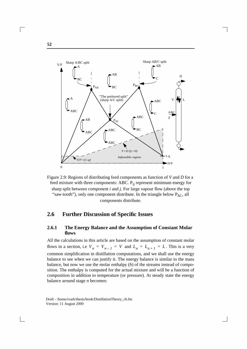
Figure 2.9 shows an example of how the components are distributed to the prod-ucts for a ternary (ABC) mixture. We choose the overhead vapour flow (V=VT)and the distillate product flow (D=V-L) as the two degrees of freedom. Thestraight lines, which are at the boundaries when a component is at the limit ofappearing/disappearing (distribute/not distribute) in one of the products, can becomputed directly by Underwood’s method. Note that the two peaks (PAB andPBC) gives us the minimum vapour flow for sharp split between A/B and B/C. Thepoint PAC, however, is at the minimum vapour flow for sharpA/C split and this occurs for a specific distribution of the intermediate B, knownas the “preferred split”.

Kings’s minimum reflux expression is only valid in the triangle below the pre-ferred split, while the Underwood equations can reveal all component recoveriesfor all possible operating points. (The shaded area is not feasible since all liquidand vapour streams above and below the feed have to be positive).

52


Figure 2.9: Regions of distributing feed components as function ofV andD for afeed mixture with three components: ABC. Pij represent minimum energy forsharp split between componenti and j. For large vapour flow (above the top“saw-tooth”), only one component distribute. In the triangle below PAC, all

components distribute.

2.6 Further Discussion of Specific Issues

2.6.1 The Energy Balance and the Assumption of Constant Molarflows

All the calculations in this article are based on the assumption of constant molarflows in a section, i.e and . This is a very

common simplification in distillation computations, and we shall use the energybalance to see when we can justify it. The energy balance is similar to the massbalance, but now we use the molar enthalpy (h) of the streams instead of compo-sition. The enthalpy is computed for the actual mixture and will be a function ofcomposition in addition to temperature (or pressure). At steady state the energybalance around stagen becomes:

0 1

V/F

D/F

1-q

PAC

PABPBC

ABC

D

V L

V=D (L=0)

ABC

AB

ABC

A

BC

A

BC

AB

C

ABC

C

AB

BC

ABC

ABC

ABC

“The preferred split”

Sharp A/BC split Sharp AB/C split

(sharp A/C split)

Infeasible regionV/F=(1-q)

F

Vn Vn 1– V= = Ln Ln 1+ L= =

2.6 Further Discussion of Specific Issues 53


(2.58)

Combining this energy balance with the overall material balance on a stage( whereW is the net total molar flow through a

section, i.e.W=D in the top section and -W=B in the bottom section) yields:

(2.59)

From this expression we observe how the vapour flow will vary through a sectiondue to variations in heat of vaporization and molar enthalpy from stage to stage.

We will now show one way of deriving the constant molar flow assumption:

1. Chose the reference state (whereh=0) for each pure component as saturatedliquid at a reference pressure. (This means that each component has a dif-ferent reference temperature, namely its boiling point ( ) at the

reference pressure.)

2. Assume that the column pressure is constant and equal to the referencepressure.

3. Neglect any heat of mixing such that .

4. Assume that all components have the same molar heat capacitycPL.

5. Assume that the stage temperature can be approximated by

. These assumptions gives on all stages and

the equation (2.59) for change in boilup is reduced to:

(2.60)

6. The molar enthalpy in the vapour phase is given as:

where is the

heat of vaporization for the pure component at its reference boiling temper-ature ( ).

LnhL n, Vn 1– hV n 1–,– Ln 1+ hL n 1+, VnhV n,–=

Vn 1– Ln– Vn Ln 1+– W= =

Vn Vn 1–

hV n 1–, hL n,–

hV n, hL n 1+,–------------------------------------ W

hL n, hL n 1+,–

hV n, hL n 1+,–------------------------------------+=

Tbpi

hL n, xi n, cPLi Tn Tbpi–( )i∑=

Tn xi n, Tbpii∑= hL n, 0=

Vn Vn 1–

hV n 1–,hV n,

------------------=

hV n, xi n, Hbpivap∆

i∑ xi n, cPVi Tn Tbpi–( )i∑+= Hbpi

vap∆

Tbpi

54


7. We assume thatcPV is equal for all components, and then the second sum-mation term above will become zero, and we have:

.

8. Then if is equal for all components we get

, and thereby constant molar flows:

and also .

At first glance, these assumptions may seem restrictive, but the assumption ofconstant molar flows actually holds well for many industrial mixtures.

In a binary column where the last assumption about equal is not fulfilled,

a good estimate of the change in molar flows from the bottom (stage1) to the top(stageN) for a case with saturated liquid feed (q=1) and close to pure products, is

given by: . The molar heats of vaporization is taken at

the boiling point temperatures for the heavy (H) and light (L) componentsrespectively.

Recall that the temperature dependency of the relative volatility were related todifferent heat of vaporization also, thus the assumptions of constant molar flowsand constant relative volatility are closely related.

2.6.2 Calculation of Temperature when Using Relative Volatilities

It may look like that we have lost the pressure and temperature in the equilibriumequation when we introduced the relative volatility. However, this is not the casesince the vapour pressure for every pure component is a direct function of temper-ature, thus so is also the relative volatility. From the relationship

we derive:

(2.61)

Remember that only one ofP or T can be specified when the mole fractions arespecified. If composition and pressure is known, a rigorous solution of the tem-perature is found by solving the non-linear equation:

(2.62)

hV n, xi n, Hbpivap∆

i∑=

Hbpivap∆ H

vap∆=

hV n, hV n 1–, Hvap∆= =

Vn Vn 1–= Ln Ln 1+=

Hbpivap∆

VN V1⁄ HHvap∆ HL

vap∆⁄≈

P pi∑ xi pio

T( )∑= =

P pro

T( ) xiαii

∑=

P xi pio

T( )∑=

2.6 Further Discussion of Specific Issues 55


However, if we use the pure components boiling points (Tbi), a crude and simpleestimate can be computed as:

(2.63)

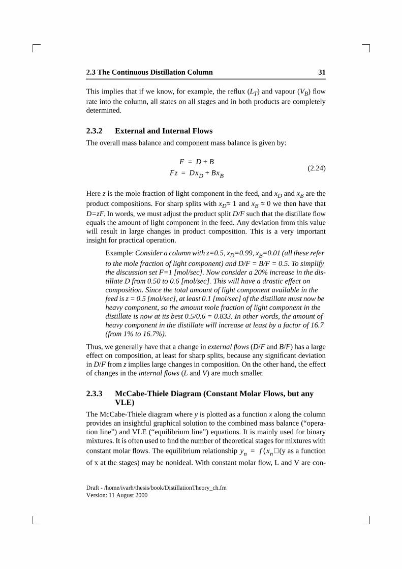
For ideal mixtures, this usually give an estimate which is a bit higher than the realtemperature, however, similar approximation may be done by using the vapourcompositions (y), which will usually give a lower temperature estimate. Thisleads to a good estimate when we use the average of x and y, i.e:

(2.64)

Alternatively, if we are using relative volatilities we may find the temperature viathe vapour pressure of the reference component. If we use the Antoine equation,then we have an explicit equation:

where (2.65)

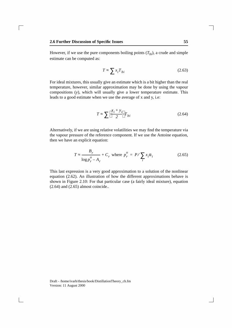
This last expression is a very good approximation to a solution of the nonlinearequation (2.62). An illustration of how the different approximations behave isshown in Figure 2.10: For that particular case (a fairly ideal mixture), equation(2.64) and (2.65) almost coincide..

T xiTbi∑≈

Txi yi+

2---------------

Tbi∑≈

TBr

pro

log Ar–-------------------------- Cr+≈ pr

oP xiαi

i∑⁄=

56


Figure 2.10: Temperature profile for the example in Figure 2.7 (solid line)compared with various linear boiling point approximations.

In a rigorous simulation of a distillation column, the mass and energy balancesand the vapour liquid equilibrium (VLE) have to be solved simultaneously for allstages. The temperature is then often used as an iteration parameter in order tocompute the vapour-pressures in VLE-computations and in the enthalpy compu-tations of the energy balance.

2.6.3 Discussion and Caution

Most of the methods presented in this article are based on ideal mixtures and sim-plifying assumptions about constant molar flows and constant relative volatility.Thus there are may separation cases for non-ideal systems where these methodscannot be applied directly.

However, if we are aware about the most important shortcomings, we may stilluse these simple methods for shortcut calculations, for example, to gain insight orcheck more detailed calculations.

0 5 10 15 20 25 30 35 40300

301

302

303

304

305

306

307

308

309

310

Bottom Stages Top

Tem

pera

ture

[K] α=1.50

z=0.50q=1.00N=40N

F=21

xDH

=0.1000x

BL=0.0020

T=Σ xiT

bi

T=Σ yiT

bi

T=Σ (yi+x

i)T

bi/2

T=f(x,P)

2.7 Bibliography 57


2.7 Bibliography

[1] Franklin, N.L. Forsyth, J.S. (1953), The interpretation of Minimum RefluxConditions in Multi-Component Distillation.Trans IChemE,Vol 31,1953. (Reprinted in Jubilee Supplement -Trans IChemE,Vol 75, 1997).

[2] King, C.J. (1980), second Edition, Separation Processes.McGraw-Hill,Chemical Engineering Series, ,New York.

[3] Kister, H.Z. (1992), Distillation Design.McGraw-Hill, New York.

[4] McCabe, W.L. Smith, J.C. Harriot, P. (1993), Fifth Edition, Unit Opera-tions of Chemical Engineering.McGraw-Hill, Chemical EngineeringSeries,New York.

[5] Shinskey, F.G. (1984), Distillation Control - For Productivity and EnergyConservation.McGraw-Hill, New York.

[6] Skogestad, S. (1997), Dynamics and Control of Distillation Columns - ATutorial Introduction.Trans. IChemE,Vol 75, Part A, p539-562.

[7] Stichlmair, J. James R. F. (1998), Distillation: Principles and Practice.Wiley,

[8] Underwood, A.J.V. (1948), Fractional Distillation of Multi-ComponentMixtures.Chemical Engineering Progress,Vol 44, no. 8, 1948

58


Distillation Theory

Documents

Transcript of Distillation Theory