Technological University Dublin Technological University Dublin

ARROW@TU Dublin ARROW@TU Dublin

Doctoral Science

2019

Distance,Time and Terms in First Story Detection Distance,Time and Terms in First Story Detection

Fei Wang Technological University Dublin

Follow this and additional works at: https://arrow.tudublin.ie/sciendoc

Part of the Computer Engineering Commons

Recommended Citation Recommended Citation Wang, F. (2019) Distance,Time andTerms in First Story Detection, Doctoral Thesis, Technological University Dublin. doi:10.21427/spp0-zx14

This Theses, Ph.D is brought to you for free and open access by the Science at ARROW@TU Dublin. It has been accepted for inclusion in Doctoral by an authorized administrator of ARROW@TU Dublin. For more information, please contact arrow.admin@tudublin.ie, aisling.coyne@tudublin.ie.

This work is licensed under a Creative Commons Attribution-Noncommercial-Share Alike 4.0 License

Distance, Time and Terms in FirstStory Detection

by

Fei Wang

Supervisors: Dr. Robert J. RossProf. John D. Kelleher

SCHOOL OF COMPUTER SCIENCE

Technological Universi ty Dublin

Thesis submitted for the degree of

Doctor of Philosophy

November 2019

Declaration

I certify that this thesis which I now submit for examination for the

award of Doctor of Philosophy, is entirely my own work and has not

been taken from the work of others, save and to the extent that such

work has been cited and acknowledged within the text of my work.

This thesis was prepared according to the regulations for postgraduate

study by research of the Technological University Dublin and has not

been submitted in whole or in part for an award in any other Institute or

University.

The work reported on in this thesis conforms to the principles and re-

quirements of the TU Dublin’s guidelines for ethics in research.

TU Dublin has permission to keep, to lend or to copy this thesis in whole

or in part, on condition that any such use of the material of the thesis be

duly acknowledged.

Signature: Date:

i

Acknowledgements

I would like to express my deepest appreciation to my supervisors,

Dr. Robert J. Ross and Prof. John D. Kelleher for their continuous guid-

ance and encouragement during my study. Robert, who gave me the

opportunity to start this, has always been there with patience and optim-

ism when I met any problem in research and life; John, who impressed

me with his immense knowledge again and again, can always provide

me with new perspectives of thinking. It was both of them who made

me a qualified researcher, and I have no doubt that without them I could

never have obtained all these achievements.

Besides my supervisors, I would like to thank Technological Univer-

sity Dublin for providing me with the excellent research environment in

Focas institute. I also would like to thank CeADAR and ADAPT for

funding my study in the first year and the following three years respect-

ively.

My sincere thanks also goes to Prof. Sarah Jane Delany, who led me

to the opportunity to start my research, and Dr. Brian Mac Namee, who

supervised my first-year study and following whose work, I took the first

step in research.

In addition, I would like to thank all my colleagues in AIRC - Gian-

ii

carlo, Ivan, Eoin, Xinlu, Guanhong, Hao, Caroline, Alex, Hector, Jack,

Pierre, Lucas, Patricia, Patrick, Andrei, Senja, Elizabeth, Annika, Irene,

Tamara, André, Bojan, Abhijit, Vihanga, Filip, Xuehao, Kaiqiang, Pal-

lavi, and especially those who made the reading (and drinking) group so

enjoyable every Friday evening.

I also want to express a special thanks to Prof. Bing Wu and Cindy

Liu for their kindness and support to my family since I arrived here.

I will also forever be thankful to Yan, Jianhua, Zenan, Qian, Meng

and Modan for their friendship, and Yupeng, Haoran, Jing, Bomao and

Rongchen for their help when I was in difficulties.

Finally, and most importantly, I would like to thank my family for

their unconditional love. I owe it all to them.

iii

Abstract

First Story Detection (FSD) is an important application of online

novelty detection within Natural Language Processing (NLP). Given a

stream of documents, or stories, about news events in a chronological

order, the goal of FSD is to identify the very first story for each event.

While a variety of NLP techniques have been applied to the task, FSD

remains challenging because it is still not clear what is the most crucial

factor in defining the “story novelty”.

Given these challenges, the thesis addressed in this dissertation is that

the notion of novelty in FSD is multi-dimensional. To address this, the

work presented has adopted a three dimensional analysis of the relative

qualities of FSD systems and gone on to propose a specific method that

we argue significantly improves understanding and performance of FSD.

FSD is of course not a new problem type; therefore, our first dimen-

sion of analysis consists of a systematic study of detection models for

first story detection and the distances that are used in the detection mod-

els for defining novelty. This analysis presents a tripartite categorisa-

tion of the detection models based on the end points of the distance

calculation. The study also considers issues of document representation

explicitly, and shows that even in a world driven by distributed repres-

iv

entations, the nearest neighbour detection model with TF-IDF document

representations still achieves the state-of-the-art performance for FSD.

We provide analysis of this important result and suggest potential causes

and consequences.

Events are introduced and change at a relatively slow rate relative

to the frequency at which words come in and out of usage on a docu-

ment by document basis. Therefore we argue that the second dimen-

sion of analysis should focus on the temporal aspects of FSD. Here we

are concerned with not only the temporal nature of the detection pro-

cess, e.g., the time/history window over the stories in the data stream,

but also the processes that underpin the representational updates that

underpin FSD. Through a systematic investigation of static representa-

tions, and also dynamic representations with both low and high update

frequencies, we show that while a dynamic model unsurprisingly out-

performs static models, the dynamic model in fact stops improving but

stays steady when the update frequency gets higher than a threshold.

Our third dimension of analysis moves across to the particulars of

lexical content, and critically the affect of terms in the definition of story

novelty. We provide a specific analysis of how terms are represented for

FSD, including the distinction between static and dynamic document

representations, and the affect of out-of-vocabulary terms and the spe-

cificity of a word in the calculation of the distance. Our investigation

showed that term distributional similarity rather than scale of common

v

terms across the background and target corpora is the most important

factor in selecting background corpora for document representations in

FSD. More crucially, in this work the simple idea of the new terms

emerged as a vital factor in defining novelty for the first story.

Motivated by the findings from our multi-dimensional analysis, we

have also developed and contributed a New Term Rate (NTR) method

for FSD, which is based on the proportion of new terms in a candidate

story given a history window. We demonstrate how this NTR method

can significantly improve the performance of FSD systems with a variety

of detection models and document representations in different types of

target corpora. Moreover, and critically, we show that deep learning-

based distributed document representations can also be used to achieve

very good detection performance with the NTR method.

vi

Contents

1 Introduction 1

1.1 Research Hypotheses . . . . . . . . . . . . . . . . . . 6

1.2 Contributions . . . . . . . . . . . . . . . . . . . . . . 7

1.3 Chapter Structure . . . . . . . . . . . . . . . . . . . . 10

1.4 Publications . . . . . . . . . . . . . . . . . . . . . . . 12

2 First Story Detection 14

2.1 Online Novelty Detection . . . . . . . . . . . . . . . . 15

2.2 Topic Detection and Tracking Project Series . . . . . . 16

2.3 First Story Detection . . . . . . . . . . . . . . . . . . 19

2.3.1 Fundamental Concepts . . . . . . . . . . . . . 20

2.3.2 Novelty Score . . . . . . . . . . . . . . . . . . 21

2.4 Target Corpora . . . . . . . . . . . . . . . . . . . . . 22

2.4.1 TDT5 Corpus . . . . . . . . . . . . . . . . . . 22

2.4.2 Twitter Corpus . . . . . . . . . . . . . . . . . 24

2.5 Evaluation . . . . . . . . . . . . . . . . . . . . . . . . 26

2.5.1 Annotated Data for Evaluation . . . . . . . . . 26

2.5.2 Gold Standard for Evaluation . . . . . . . . . 27

2.5.3 False Alarm Rate and Miss Rate . . . . . . . . 28

2.5.4 Detection Error Trade-off Curve and Area Un-

der Curve Score . . . . . . . . . . . . . . . . . 29

vii

2.5.5 Detection Cost . . . . . . . . . . . . . . . . . 31

2.6 Detection Models . . . . . . . . . . . . . . . . . . . . 33

2.6.1 Information Retrieval-Based Detection Models 33

2.6.2 Nearest Neighbour-Based Detection Models . . 38

2.6.3 Other General Detection Models . . . . . . . . 41

2.6.4 Detection Models for Specific Purposes . . . . 44

2.6.5 Improving Methods . . . . . . . . . . . . . . . 45

2.7 Discussion . . . . . . . . . . . . . . . . . . . . . . . . 47

2.8 Summary . . . . . . . . . . . . . . . . . . . . . . . . 48

3 Detection Model Categorisation and Analysis 50

3.1 Three Categories of Detection Models . . . . . . . . . 51

3.2 Comparisons across Different Categories . . . . . . . . 56

3.2.1 Experimental Design . . . . . . . . . . . . . . 57

3.2.2 Experimental Results . . . . . . . . . . . . . . 59

3.3 Comparisons across Different Document Representations 60

3.3.1 Distributed Document Representations . . . . 61

3.3.2 Experiments . . . . . . . . . . . . . . . . . . 66

3.4 Discussion . . . . . . . . . . . . . . . . . . . . . . . . 70

3.5 Summary . . . . . . . . . . . . . . . . . . . . . . . . 72

4 Background Corpus Selection and Evaluation 73

4.1 Static TF-IDF Model for First Story Detection . . . . . 76

viii

4.2 Quantitatively Measuring Background Corpus

Suitability . . . . . . . . . . . . . . . . . . . . . . . . 79

4.2.1 Measuring the Scale of Common Terms . . . . 79

4.2.2 Measuring the Distributional Similarity . . . . 79

4.2.3 Comparison between Two Background Corpora

Relative to a Target Corpus . . . . . . . . . . . 82

4.3 Experimental Design . . . . . . . . . . . . . . . . . . 83

4.3.1 Corpora Used in the Experiments . . . . . . . 84

4.3.2 Metric Calculation . . . . . . . . . . . . . . . 86

4.3.3 Evaluation of Detection Performance . . . . . 86

4.4 Results and Analysis . . . . . . . . . . . . . . . . . . 88

4.4.1 Results of the Comparisons of Corpus Dissimil-

arity . . . . . . . . . . . . . . . . . . . . . . . 88

4.4.2 Results of the Relations between Background

Corpus and Model Performance . . . . . . . . 90

4.5 Discussion . . . . . . . . . . . . . . . . . . . . . . . . 90

4.6 Summary . . . . . . . . . . . . . . . . . . . . . . . . 92

5 Dynamic Model Updates for First Story Detection 94

5.1 Dynamic TF-IDF Models for First Story Detection . . 97

5.2 Experimental Design and Results . . . . . . . . . . . . 101

5.2.1 Experimental Design . . . . . . . . . . . . . . 101

ix

5.2.2 Comparisons across Different Update Frequen-

cies . . . . . . . . . . . . . . . . . . . . . . . 102

5.2.3 Comparisons across Different Background Cor-

pora . . . . . . . . . . . . . . . . . . . . . . . 104

5.2.4 Comparisons across Mini Corpora . . . . . . . 105

5.3 Discussion . . . . . . . . . . . . . . . . . . . . . . . . 107

5.3.1 Effect of Rough Terms in the Calculations . . . 107

5.3.2 Exploration on the Usage of Rough Terms . . . 112

5.4 Summary . . . . . . . . . . . . . . . . . . . . . . . . 114

6 The New Term Rate Method 116

6.1 Motivation . . . . . . . . . . . . . . . . . . . . . . . . 117

6.2 The New Term Rate Method . . . . . . . . . . . . . . 118

6.2.1 Newe Term Rate . . . . . . . . . . . . . . . . 119

6.2.2 The New Term Rate Method . . . . . . . . . . 119

6.2.3 Method Properties . . . . . . . . . . . . . . . 121

6.2.4 The Distinct New Term Rate Method . . . . . 123

6.3 Experimental Verification . . . . . . . . . . . . . . . . 125

6.3.1 Experimental Design . . . . . . . . . . . . . . 125

6.3.2 Results for Reference . . . . . . . . . . . . . . 126

6.3.3 Verification in Different Background Corpora . 128

6.3.4 Verification in Different Types of Document Re-

presentations . . . . . . . . . . . . . . . . . . 133

x

6.3.5 Verification in Different Types of Detection Mo-

dels . . . . . . . . . . . . . . . . . . . . . . . 135

6.3.6 Verification in Different Types of Target Corpora 137

6.4 Discussion . . . . . . . . . . . . . . . . . . . . . . . . 138

6.4.1 Selection of History k . . . . . . . . . . . . . 140

6.4.2 Selection of NTR Weight α . . . . . . . . . . 142

6.5 Summary . . . . . . . . . . . . . . . . . . . . . . . . 145

7 Conclusions 146

7.1 Summary of Contributions . . . . . . . . . . . . . . . 147

7.2 Directions for Future Work . . . . . . . . . . . . . . . 150

xi

List of Figures

2.1 Example DET curves . . . . . . . . . . . . . . . . . . 30

3.1 FSD performances across different categories of models 60

3.2 FSD performances across different document represent-

ations for P2P models . . . . . . . . . . . . . . . . . . 68

3.3 FSD performances across different document represent-

ations for P2C models . . . . . . . . . . . . . . . . . . 68

3.4 FSD performances across different document represent-

ations for P2A models . . . . . . . . . . . . . . . . . 69

4.1 Term sets within a background Corpus B and a target

Corpus T . . . . . . . . . . . . . . . . . . . . . . . . 77

4.2 Common Set among two background Corpus B1 and B2

and a target Corpus T . . . . . . . . . . . . . . . . . . 84

4.3 Comparisons of corpus dissimilarity . . . . . . . . . . 89

5.1 Comparisons across different update frequencies and b-

ackground corpora . . . . . . . . . . . . . . . . . . . 103

5.2 Comparisons across mini background corpora with the

update frequency set as every 500 stories . . . . . . . . 106

6.1 Two types of correspondences between the history k and

the FSD performance . . . . . . . . . . . . . . . . . . 142

xii

6.2 Two types of correspondences between the NTR weight

α and the FSD performance . . . . . . . . . . . . . . . 144

xiii

List of Tables

2.1 Confusion matrix . . . . . . . . . . . . . . . . . . . . 28

3.1 AUC scores across different document representations

in different categories of models . . . . . . . . . . . . 69

4.1 Comparisons between COCA and COHA . . . . . . 91

4.2 Comparisons between COCA and COCA_After_2003 91

4.3 Comparisons between COCA_News and COCA_Ex-

cept_News . . . . . . . . . . . . . . . . . . . . . . . 91

5.1 Two document representation vectors based on a dy-

namic TF-IDF model . . . . . . . . . . . . . . . . . . 98

5.2 Different situations when comparing an incoming story

with an existing story . . . . . . . . . . . . . . . . . . 111

6.1 The state-of-the-art FSD results for the TDT5 and Twit-

ter target corpora . . . . . . . . . . . . . . . . . . . . 127

6.2 Best results of pure NTR FSD system for different target

corpora. . . . . . . . . . . . . . . . . . . . . . . . . . 127

6.3 The effectiveness of the NTR method in the nearest ne-

ighbour model with the TF-IDF document representa-

tions for the TDT5 target corpus . . . . . . . . . . . . 130

6.4 The comparison between the effectiveness of the NTR

method and the distinct NTR method . . . . . . . . . . 133

xiv

6.5 The effectiveness of the NTR method in the nearest ne-

ighbour model with different types of document repres-

entations for the TDT5 target corpus . . . . . . . . . . 136

6.6 The effectiveness of the NTR method in different FSD

models for the TDT5 target corpus . . . . . . . . . . . 136

6.7 The effectiveness of the NTR method in Twitter target

corpus . . . . . . . . . . . . . . . . . . . . . . . . . . 139

xv

Chapter 1

Introduction

First Story Detection (FSD), also called New Event Detection, is a very

important application of online novelty detection within Natural Lan-

guage Processing (NLP) (Allan et al., 1999). Given a stream of docu-

ments, or stories, about news events in a chronological order, the goal

of FSD is to identify the very first story for each event (Fiscus and Dod-

dington, 2002). Each story is processed in sequence, and a decision is

made for a given candidate story on whether or not it discusses an event

that has not been seen in previous stories; crucially this decision is made

after processing the candidate document but before processing any sub-

sequent documents (Allan et al., 1998b; Yang et al., 1998).

As the fast-growing amount of digital content overwhelms human

attention, it becomes impossible for people to manually handle all the

information from news medias or social networks. From The Atlantic

(2016), it is reported that The Washington Post publishes an average

of 1,200 stories, graphics, and videos per day; NYTimes.com publishes

1

roughly 150-250 articles per day; while Times, The Wall Street Journal,

and BuzzFeed.com publish about 230, 240, and 222 pieces of content

daily. On social media meanwhile, the values are more staggering; take

for example Twitter, where on average 500 million tweets are sent per

day, according to the last time official statistics were released in 2014

(Business of Apps, 2019). In this situation, the need for an intelligent

detection system is all the more vital.

Standard topic detection and modelling methods take a retrospective

view on detection, i.e., they find topics after the full set of documents are

processed, and consequently, timeliness of the detection usually cannot

be achieved (Yang et al., 1998; Steyvers and Griffiths, 2007). However,

for certain organisations and people, there is a benefit to be first to learn

about new events, and thus the lagging retrospective detection methods

cannot satisfy their needs. For example, a news outlet always wants to

get the breaking news before their competitors, and a quantitative trading

firm expects to make decisions with the facilitation of real-time breaking

news. From this perspective, an online system to detect the first story for

each new event is essential.

In general, compared to other related tasks like topic detection or

topic tracking, FSD is widely considered to be the more difficult task

(Allan et al., 2000b). The challenges in building an acceptable FSD

system come from a variety of perspectives:

- Unsupervised. Unlike in supervised learning applications where

2

the learning process is based on labelled data, there is no labelled

training data available in FSD (Wayne, 1997). In other words, there

is not an explicit idea of what the next event, or its first story, is

like, and thus, FSD is normally considered to be an unsupervised

learning application, in which detection can only be made with the

intrinsic properties of the stories.

- Online. As an application of online novelty detection, FSD inherits

the online characteristic. In FSD, detection can only be implemen-

ted based on the stories that have already arrived, and the decision

making process must be fast, e.g., before the next story arrives

(Yang et al., 1998). Traditional topic modelling approaches, such

as latent semantic indexing (LSA) (Papadimitriou et al., 2000), lat-

ent Dirichlet allocation (LDA) (Blei et al., 2003), and clustering

algorithms like k-means (Hartigan, 1975) and agglomerative clus-

tering(Jain and Dubes, 1988), require the entire corpus to find the

latent topics in documents, and therefore are not suitable for FSD.

- Fine-grained. Within the context of NLP, the event to be detected

in FSD is limited to a specific scope - “something that happens at

a particular time and place” (Papka et al., 1998). For example, the

Boeing 737 MAX airplane crashes in Indonesia and Ethiopia are

two different events for FSD, although they are in the same gen-

eral topic, “airplane crash”. This fine-grained event scope makes it

3

impossible to pre-define target events from general topics, and also

brings in the difficulty of distinguishing events in the same general

topic that share similar words.

Given these challenges, many detection systems have been proposed

for FSD. Early research took this task as a special Information Retrieval

(IR) task, and applied traditional IR methods like filtering or tracking

systems to solve this problem (DeJong, 1979; Belkin and Croft, 1992;

Callan et al., 1996; Zhang et al., 2002). In UMass (Allan et al., 2000c)

and CMU (Yang et al., 1998), the two IR-based systems designed spe-

cifically for FSD, a query is built with a single existing story or a cluster

of existing stories, and the degree of mismatching between the incoming

story and its closest query is considered to be the novelty of the incom-

ing story.

Additionally, in both UMass and CMU systems, the way to build

queries based on a single existing story achieved better performance than

that based on a cluster of existing stories, which indicated that nearest

neighbour-based detection models outperform clustering-based model

for FSD. Thus, a series of following research chose the nearest neigh-

bour model as the research focus and designed a variety of methods to

improve the detection performance. Petrovic et al. (2010b) took the FSD

task as an approximate nearest neighbour problem and developed the

FSD model with locality sensitive hashing (LSH) (Indyk and Motwani,

1998; Lv et al., 2007) that improves the efficiency of FSD significantly

4

and thus makes it possible to apply FSD to very large social network

datasets like Twitter data. Then, Petrovic et al. (2012) and Moran et al.

(2016) extended the LSH FSD model by using paraphrases to alleviate

the lexical variation problem and achieved the state of the art in different

corpora.

In recent years, with the development of user generated content

(UGC), many FSD systems focused on the FSD application to social

media. Wurzer et al. (2015) and Wurzer and Qin (2018) proposed the

k-term hashing FSD model in which the incoming story is compared to

a look-up table of all the up-to-k terms from existing stories, and val-

idated its effectiveness in Twitter data. Qiu et al. (2015, 2016) used

special properties of Twitter data like the “@” and hashtag to build the

“nuggets” of events, and achieved very good FSD performance in Twit-

ter data.

Based on the research introduced above, we can see that although

a variety of solutions have been proposed for the FSD task, the vast

majority tend to apply different types of models and methods to get bet-

ter performance, but few focus on an analysis of the reason for which

a model or method might improve or harm detection. We believe the

key problem that underlies all these and makes FSD still challenging is

that it is not clear what is the most crucial factor in defining the “story

novelty”. Indeed, even outside of FSD, a transparent definition of the

research target is essential for any other typical unsupervised learning

5

application (Zaki et al., 2014).

1.1 Research Hypotheses

For this dissertation, we propose our hypotheses: 1) the clear exposition

of the definition of novelty should be the basis of designing a proper de-

tection model and enhancing its performance; 2) the notion of novelty is

multi-dimensional in FSD and thus a comprehensive analysis from the

perspectives of distance, time and terms can help with the understand-

ing of the task and also the design of new methods for improving the

performance of FSD systems.

In order to test these hypotheses, in this dissertation we present a

three dimensional analysis, and move on to propose a specific method

that we argue significantly improves our understanding and performance

of FSD. Our first dimension of analysis consists of a systematic study of

detection models for FSD and the distances that are used in the detection

models for defining novelty. A tripartite categorisation of the detection

models is proposed based on different types of distances used in defining

novelty scores. The second dimension of our investigation is focused on

the temporal nature of FSD, not only of the detection process but also

of the document representation models. Through a systematic investiga-

tion of static and dynamic representation models, we show that dynamic

models with high update frequencies outperform the static model and

6

dynamic models with low update frequencies, and the dynamic model

stops improving but stays steady when the update frequency gets higher

than a certain threshold. The third dimension of analysis moves across

to the specifics of lexical content, and critically the affect of terms in the

definition of story novelty. From this investigation, we found that new

terms are a vital factor in defining novelty for the first story.

Based on the findings from our multi-dimensional analysis, we are

able to propose an efficient and straightforward method based on the

proportion of new terms in a candidate story given a history window,

which we show significantly improves the performance of FSD systems

with a variety of detection models and document representations in dif-

ferent types of target corpora.

1.2 Contributions

This thesis makes the following contributions:

1. We propose a new categorisation of detection models for FSD ba-

sed on different definitions of novelty scores, and demonstrate that

the nearest neighbour-based Point-to-Point (P2P) models generally

outperform the Point-to-Cluster (P2C) models and the Point-to-All

(P2A) models.

2. We are the first to apply deep learning-based distributed document

representations to FSD. Additionally, we demonstrate that the tra-

7

ditional term vector document representation like the TF-IDF rep-

resentation, outperforms deep learning-based distributed document

representations, and argue that one potential reason for this may be

that the word specificity is well retained by the term vector repres-

entations.

3. We make elaborate theoretical analysis on the most effective FSD

system - the nearest neighbour models with the TF-IDF document

representations, and determine the factors of the TF-IDF models

that influence FSD performance: the scale of common terms and

the distributional similarity between the background and target cor-

pora for static TF-IDF models; and the update frequency for dy-

namic TF-IDF models.

4. We propose a set of metrics to quantitatively measure the scale of

common terms (i.e., inversion count and Manhattan distance) and

the distributional similarity (i.e., overlapping rate) between cor-

pora, and also provide a pairwise comparison scheme between two

different background corpora relative to a target corpus.

5. We apply our proposed metrics and comparison scheme to the com-

parisons between background corpora for static TF-IDF models,

and indicate that term distributional similarity is more predictive of

good FSD performance than the scale of common terms, and thus

a smaller recent domain-related corpus will be more suitable than a

8

very large-scale general corpus for the application of static TF-IDF

models to FSD.

6. We empirically validate that dynamic TF-IDF models with high up-

date frequencies outperform the static model and dynamic models

with low update frequencies. We also find that the FSD perform-

ance of dynamic models does not always improve but stays steady

as the update frequency goes beyond some threshold, and that the

background corpora have very limited influence on the dynamic

models with high update frequencies in terms of FSD performance.

Therefore, we make the conclusion that the effective term vector

model for FSD should be a dynamic model whose weights are ini-

tially calculated based on any small-size corpus but updated with a

reasonable high frequency, e.g., for our scenario we find an update

frequency of every 500 stories to result in good performance.

7. We set out some factors that may explain our findings in the TF-

IDF models, most importantly, the new terms with roughly-calcul-

ated large weights, which can help explain not only why the dy-

namic TF-IDF models perform best for FSD, but also why the FSD

performance of dynamic models does not always improve but stays

steady as the update frequency goes beyond some threshold.

8. We finally propose an efficient and straightforward New Term Rate

(NTR) method that can be generally applied to a wide range of

9

FSD systems without modification to the original detection models

but can improve their performances significantly. We demonstrate

that for the very large-scale Twitter corpus, with our proposed NTR

method the nearest neighbour model with the distributed document

representations achieves competitive or better FSD performance

compared to the state of the art.

We believe that the aforementioned contributions, especially our pro-

posed NTR method, can generally improve the overall level of FSD, and

can provide insights to researchers working in related novelty focused

domains.

1.3 Chapter Structure

The main body of this thesis is structured as follows:

- Chapter 2 illustrates the origin, definition, history and existing re-

search on the FSD task, and expands on the main research prob-

lem for our current research. Furthermore, the corpora, evaluation

methods and further matters needing attention in this thesis are also

presented in Chapter 2.

- Chapter 3 proposes our new categorisation of FSD models based

on different definitions of novelty scores, and provides experimen-

tal analysis of different categories of FSD models with different

types of document representations.

10

- Chapter 4 investigates how the nearest neighbour model with the

static TF-IDF document representation works for FSD, and ana-

lyses two key factors of background corpora for a static TF-IDF

model that influence the performance of FSD.

- Chapter 5 looks into the nearest neighbour model with dynamic

TF-IDF document representations to determine the proper way to

select update frequency and background corpus for the dynamic

TF-IDF models, and reveals the key factor that may lead to the

outstanding performance of the dynamic TF-IDF models: the new

terms with roughly-calculated large weights.

- Chapter 6 defines the new term rate for a candidate story and pro-

poses a generalisable method for improving FSD systems: the New

Term Rate (NTR) method. The experimental analysis in Chapter 6

also verifies the effectiveness of the NTR method in a wide range

of FSD systems.

- Chapter 7 draws conclusions by summarising our contributions in

this dissertation and pointing out some potential research directions

in which our work may be extended in the future.

11

1.4 Publications

The work presented in this dissertation has been published as a series of

papers. These are summarised below.

• Chapter 3. Wang, F., Ross, R. J., & Kelleher, J. D. (2018). Explor-

ing Online Novelty Detection Using First Story Detection Models.

In International Conference on Intelligent Data Engineering and

Automated Learning (pp. 107-116). Springer, Cham.

• Chapter 4. Wang, F., Ross, R. J., & Kelleher, J. D. (2019a). Big-

ger versus Similar: Selecting a Background Corpus for First Story

Detection based on Distributional Similarity. In Recent Advances

in Natural Language Processing.

• Chapter 5. Wang, F., Ross, R. J., & Kelleher, J. D. (2019b). Up-

date Frequency and Background Corpus Selection in Dynamic TF-

IDF Models for First Story Detection. In International Conference

of the Pacific Association for Computational Linguistics.

• Chapter 6. Wang, F., Ross, R. J., & Kelleher, J. D. (in prepara-

tion). New Terms: An Often Overlooked But Essential Factor for

Improving the Performance of First Story Detection.

In addition to the work presented here on FSD, preliminary work

for this dissertation was also conducted on categorical data clustering

12

and clustering evaluation. Two publications resulted from this work are

shown below.

• Wang, F., Franco-Penya, H. H., Pugh, J., & Ross, R. J. (2016). Em-

pirical Comparative Analysis of 1-of-K Coding and K-Prototypes

in Categorical Clustering. in Irish Conference on Artificial Intelli-

gence and Cognitive Science.

• Wang, F., Franco-Penya, H. H., Kelleher, J. D., Pugh, J., & Ross, R.

J. (2017). An Analysis of the Application of Simplified Silhouette

to the Evaluation of k-means Clustering Validity. In International

Conference on Machine Learning and Data Mining in Pattern Re-

cognition (pp. 291-305). Springer, Cham.

13

Chapter 2

First Story Detection

In order to explore the definition of story novelty for FSD, it is neces-

sary to have a comprehensive review of previous research as well as the

current state of the art. In this chapter, we review the origin of FSD, and

introduce the key research developments that have contributed to pro-

gress on this task. From this review, we identify a number of problems

that still exist in this research area and that limit the further progress of

FSD. This chapter can be considered as the background for all the fol-

lowing chapters that move on to make detailed analysis and discussion

of FSD from the perspectives of distance, time and terms.

The structure of this chapter is organised as follow: we start with

an introduction to online novelty detection and the Topic Detection and

Tracking (TDT) project series, the two sources where the FSD task ori-

ginated from, in Section 2.1 and 2.2, followed by the concept definitions

and key properties of the FSD task in Section 2.3. In Section 2.4 and

2.5, we present the corpora and evaluation methods commonly used for

14

FSD respectively. Then, in Section 2.6, we review a variety of previous

detection models for FSD, before discussing the existing problems in

previous research in Section 2.7. Finally, we present a summary of this

chapter in Section 2.8.

2.1 Online Novelty Detection

Novelty detection is the task of identifying data that are different in some

respect from training data (Pimentel et al., 2014). Novelty is the prop-

erty of abnormal data that usually indicates a defect (industry) (Marchi

et al., 2017; Cha and Wang, 2018; Liu et al., 2018), a fraud (business)

(Yamanishi et al., 2004; Dheepa and Dhanapal, 2009; Issa and Vasarhe-

lyi, 2011), an intrusion (security) (Yeung and Chow, 2002; Yeung and

Ding, 2003; Bivens et al., 2002), or a new topic in texts (media) (Markou

and Singh, 2003a,b; Conheady and Greene, 2017) . In most cases, there

is not an explicit definition for novelty or sufficient novel data to form

a class of novelty before detection. Instead, novelty detection is usually

treated as an unsupervised learning application, i.e., no labelled training

examples are available and the detection is implemented based on only

the intrinsic properties of the data (Pimentel et al., 2014).

Online novelty detection is a special case of novelty detection, in

which input data are time-ordered streams. The online characteristic

brings in two additional constraints (Ma and Perkins, 2003): 1) the de-

15

tection should be made quickly, e.g., before subsequent data arrives; and

2) looking forward is prohibited during detection, i.e., the detection can

only be made based on the data that has already arrived. The applic-

ation domains of online novelty detection range from sensor detection

(Gruhl et al., 2015) and automatic control system (Mounce et al., 2010)

to computer vision and robotics (Neto and Nehmzow, 2007; Sofman

et al., 2010; Ross et al., 2015). First Story Detection is the application

of online novelty detection within Natural Language Processing (NLP),

and has its own characteristics, which will be shown in the following

sections.

2.2 Topic Detection and Tracking Project Series

First Story Detection (FSD) was initially defined within Topic Detection

and Tracking (TDT), a project series funded by DARPA (Defense Ad-

vanced Research Projects Agency, U.S.)1 starting from 1996 (Wayne,

1997) and ending at 2004 (Connell et al., 2004). There are mainly five

phases in the TDT series:

- TDT1, i.e., TDT pilot study or TDT 1997 (Allan et al., 1998a);

- TDT2, i.e., TDT 1998 (Fiscus et al., 1999);

- TDT3, i.e., TDT 1999 and TDT 2000 (Fiscus and Doddington,

2000);1https://www.darpa.mil/

16

- TDT4, i.e., TDT 2001 (Braun and Kaneshiro, 2003);

- TDT5, i.e., TDT 2004 (Connell et al., 2004).

The division of TDT phases is based on different target corpora created

for use in the detection and tracking, that is, the corpora TDT1 to TDT5.

The overall goal of the TDT series is to explore technologies related

to event-based information organisation tasks in news stories (Wayne,

1997), and there are in total five specific tasks explored in it (Fiscus and

Doddington, 2002):

- Story Segmentation, which is defined to be the task of segmenting

a continuous stream of story texts into its constituent stories. The

story texts in the target corpus are concatenated as the input stream,

and the output of the segmentation system will be the locations of

the boundaries between adjacent stories for all stories in the target

corpus.

- Topic Tracking, which is the task of detecting stories discussing a

previously known event. An event is “known” by having a small

number of sample stories discussing it, and the detection is to find

all the following stories in the story stream that discuss the same

event.

- Topic Detection, which is defined as the task of identifying all the

events in the target corpus. This task requires detection systems to

17

group all the stories into topic clusters where each cluster repres-

ents a single event. The decision can be made after all the story

texts in the stream are processed.

- First Story Detection (FSD), which is the task of identifying the

very first story to discuss a new event. Given a stream of stories

in chronological order, the FSD system is required to make the

decision for each incoming candidate story whether it discusses a

previous unseen event or not.

- Story Link Detection, which is to detect whether a pair of stories are

topically linked. In other words, the goal of this task is to answer

the question: “do these two stories discuss the same topic?" The

decision needs to be made between all the story pairs in the target

corpus.

The focus of our dissertation is the First Story Detection (FSD) task,

which has close relations to other tasks (Papka, 1999): Story Segmenta-

tion and Topic Tracking are in practice the prerequisite and subsequent

task of FSD in a comprehensive topic detection and tracking process;

Topic Detection is a more general task, in which FSD is a special case

where the detection must be implemented in an online style; Topic Trac-

king and Story Link Detection can be considered as solutions to FSD, in

which the first story is identified if the incoming story cannot be tracked

by any previously known event or it does not topically link to any ex-

18

isting story. However, FSD is also considered to be more difficult than

other tasks in TDT (Allan et al., 2000b), e.g., an acceptable FSD per-

formance requires the Topic Tracking system to be almost perfect (Allan

et al., 2000a).

2.3 First Story Detection

As the application of online novelty detection to Natural Language Pro-

cessing (NLP), FSD has the common properties of online novelty de-

tection, but also some specific characteristics for NLP. On one hand,

FSD is implemented like other applications of online novelty detection,

where there is neither a clear idea of what the novel event is like, nor

sufficient information to build a class of first stories to implement super-

vised training. The detection can only be made based on the stories that

have already arrived before the candidate story arrives, and the two con-

straints for online novelty detection - “no looking forward” and “quick

decision”, also apply to FSD. On the other hand, the concept “novelty”

has special meaning for NLP. In this section, we introduce some specific

characteristics of FSD: the definitions of fundamental concepts and the

novelty scores in the detection.

19

2.3.1 Fundamental Concepts

“Event” and “story” are two fundamental but important concepts in FSD,

which restrict the target and object of detection, and thus, an explicit

definition is required for each of them.

At the beginning of the FSD research, an “event” was initially defined

as “something that happens at a particular time and place” (Papka et al.,

1998). This definition makes it differ from the concept “topic”, which

is normally considered to be a broader class of events, both in spa-

tial/temporal localisation and in specificity (Allan et al., 1998a). For

example, the Boeing 737 MAX airplane crash in Ethiopia on 10 March

2019 is an event, while airplane crash is a more general class of events

containing it, i.e., a topic. In order to reduce the confusion in definition,

the concept “topic” in TDT is modified and sharpened to be an “event”

(Allan et al., 1998a).

However, this initial definition of “event” is problematic in defining

an event like “the O.J. Simpson saga”, that may occur over years and

in many places (Allan et al., 1998b). Therefore, the definition of an

event was modified to be “a seminal event or activity, along with all

directly related events and activities” (Doddington, 1998). Stories will

be considered to be “on topic” when it is directly connected to an event.

Also taking the Boeing 737 MAX airplane crash as example, stories

about the search for survivors, or the funeral of the crash victims, will

20

all be considered to be part of the crash event; however, the following

investigation and banning of the airplane model probably would not be

considered to be part of the original crash event.

Based on this definition of “event”, the “story” in TDT is defined as

“a topically cohesive segment of news that includes two or more declar-

ative independent clauses about a single event” (Fiscus and Doddington,

2002). In this definition, there is an implicit assumption that a story only

discusses a single event.

These definitions have been accepted in the TDT project series and

all following research. In this dissertation, we also take them as the

definitions of these basic concepts.

2.3.2 Novelty Score

In true FSD systems, the output for each candidate story is not directly

“positive” or “negative”. Instead, a novelty score (or confidence score)

is normally required in the decision making process for each incoming

story, which corresponds to the probability of the story discussing a new

event. If the novelty score of the candidate story is higher than a given

threshold, we say it is a first story; otherwise, an old story. Unfortu-

nately, compared to providing a novelty score for each incoming story,

it is quite difficult to determine a good threshold before detection. Con-

sequently, the standard evaluation method for FSD systems is to apply

multiple thresholds to sweep through all the novelty scores and then find

21

out the threshold that leads to the best performance, the details of which

will be given in Section 2.5.

At this early point of the dissertation, there are two points in our re-

search that are very important to be noted: firstly, we always consider

the FSD task to be within the area of general NLP; secondly, the FSD

techniques that we investigate and develop must be able to be general-

ised to different situations rather than only for a specific case. Therefore,

in this work we focus primarily on traditional news data - because these

documents are in a more general/standard form of English - and use so-

cial media data to: (a) evaluate the generalisation ability of our systems

to different genres of English, or (b) enable direct comparison between

our results and previous research.

2.4 Target Corpora

In order to explore the satisfactory understanding of this task, some spe-

cific corpora have been proposed for FSD: the TDT corpora and the

Twitter corpus.

2.4.1 TDT5 Corpus

As mentioned in Section 2.2, five corpora were proposed during the TDT

project series, i.e., the corpora TDT1 to TDT5. All these corpora are

constituted by news stories that were collected from multiple sources

22

like newswires, radio programs and television programs within a time

window, normally, a few months (Allan et al., 1998a; Cieri et al., 1999;

Graff et al., 1999; Li et al., 2005; Connell et al., 2004). The collection

of stories and the subsequent cleaning, manipulation and annotation pro-

cesses are administrated by LDC (The Linguistic Data Consortium) (De

and Kontostathis, 2005)2.

The scale of corpus increases from only 15,863 stories in the TDT1

corpus (Allan et al., 1998a) to 407,505 stories in the TDT5 corpus (Lin-

guistic Data Consortium, 2006). From TDT3, TDT projects took into

account multilingual sources in Chinese (Cieri et al., 2000) and Arabic

(Yu et al., 2004), and evaluated the topic detection and tracking in dif-

ferent languages (Fiscus and Doddington, 2000; Wayne, 2000b,a) and

even in a cross-language way (Chen and Chen, 2002; Spitters and Kraaij,

2002; Larkey et al., 2004; Pouliquen et al., 2004).

In this dissertation, we adopt the TDT5 corpus (Linguistic Data Con-

sortium, 2006) as the main corpus for the evaluation of the performance

of FSD systems, which is the last corpus proposed in TDT and has been

widely taken as the benchmark corpus for FSD in the following research

(Kumaran and Allan, 2005; Petrovic et al., 2010b, 2012; Karkali et al.,

2013; Fu et al., 2015; Rao et al., 2017). As mentioned above, the TDT5

corpus consists of more than 400 thousand stories in English, Chinese

and Arabic. However, our research only focuses on FSD in English, so

2https://www.ldc.upenn.edu/

23

we ignore the parts of TDT5 in other languages, and only keep the Eng-

lish part, in which there are in total 278,108 English news stories col-

lected from April to September 20033. Similar to all the previous TDT

corpora, multiple-sources is also one characteristic of the TDT5 corpus.

The sources of the stories in TDT5 include Agence France Presse, As-

sociated Press, Central News Agency - Taiwan, LA Times/Washington

Post, New York Times, Ummah Press and Xinhua News Agency. All the

news stories in the corpus are ordered in the input stream by their time

stamps that were given when they were collected from these sources.

2.4.2 Twitter Corpus

Beyond its application to traditional news stories like in the TDT project

series, FSD has attracted considerable attentions in recent years with

the popularisation of social networks and user-generated content (UGC)

like Twitter. Compared with traditional news stories, the stories from

Twitter, i.e., the tweets, are also a very good fit for FSD (Petrovic et al.,

2010b): they cover far more events than would be possible in traditional

news sources; and they can be reported in almost real time, much sooner

than the news. Of course, there are also some extra problems that need

to be dealt with: the scale of data in Twitter is huge; the data is noisy

because of typos and non-standard grammars; the length of stories may

be extremely short; and the events may be very trivial (Petrovic et al.,3In the following parts of this dissertation, we will use “TDT5” or “the TDT5 corpus” to refer to

only the English part of the corpus rather than the entire corpus.

24

2012).

A specific Twitter corpus was published for FSD by researchers from

University of Edinburgh in 2010, i.e., the Edinburgh Twitter corpus (or

Twitter corpus for short) (Petrovic et al., 2010a). After removing non-

English tweets, this corpus consists of about 50 million tweets collected

from beginning of July to mid-September 2011, which is much larger

than TDT5 in terms of the number of stories. Although there are plenty

of Twitter corpora published in the area of NLP, the Edinburgh Twitter

corpus is the only one collected and annotated specifically for FSD, and

thus widely used as the benchmark corpus for FSD in Twitter (Petrovic

et al., 2012; Qiu et al., 2015; Moran et al., 2016; Wurzer and Qin, 2018).

In order to evaluate the generalisation ability of our FSD systems or

make comparison with results by previous research, we use this Twitter

corpus as a supplemental corpus.

It is worth mentioning that many Twitter-specific characteristics are

taken into account in this corpus, such as retweets, “@” tags and hasht-

ags, some of which can be naturally taken as good indicators of events

(Atefeh and Khreich, 2015). However, we only take the texts of the

tweets as plain English and do not take advantage of these special char-

acteristics of Twitter, because the decision processes based on these spe-

cial tokens can not be generalised to other types of data and thus are not

within our research focus. When we collected the texts of the Twitter

corpus in 2017, one issue came out: because in 2010 the corpus was

25

published only with the tweet IDs rather than the texts of tweets, when

we tried to download all the texts through the API provided by Twitter

with the tweet IDs, a large amount of tweets have already been deleted

or set as inaccessible. In the end, it was only possible to get 32,363,398

of 51,879,318 tweets (about 62.38% of all) in the corpus, which is nev-

ertheless still a usable large Twitter corpus for FSD. Therefore, in the

following part of the dissertation, we use the term “Twitter corpus” to

refer to this incomplete corpus.

2.5 Evaluation

In this section, we firstly explain the annotated data for evaluation in

each FSD corpora, and then introduce the evaluation methods commonly

used in this research area.

2.5.1 Annotated Data for Evaluation

The evaluation of FSD systems in this dissertation is based on the two

corpora described in the last section, i.e., the TDT5 and Twitter corpora.

However, although all the stories in each corpus are processed in detec-

tion, not all of them are used for evaluation. In fact, only a small portion

of each corpus is annotated for the evaluation: 6,636 stories, about 126

events, in the TDT5 corpus; and 2,160 stories, about 27 events, in the

Twitter corpus. The annotation of stories starts from the selection of a

26

set of target events, followed by the search for all the stories discussing

the selected target events throughout the entire corpus. Therefore, there

are stories about other events in each corpus which are considered to be

background stories and which are not taken into account in the evalu-

ation. However, the information for the evaluation is not available in the

detection process, and thus decisions need to be made for all the stories

in the corpus, but only the results for the labelled stories are used for

evaluation. Because the goal of FSD is to identify only the very first

story of each event, the number of stories with the label “positive” is the

same as the number of total target events. For example, in TDT5 there

are 126 target events and thus 126 first stories with label “positive” as

the detection targets.

2.5.2 Gold Standard for Evaluation

For the evaluation of an NLP task, people’s judgements on the detection

are normally taken as the gold standard. In FSD, the annotated labels

are taken to represent a typical persons judgements on whether a given

story is a first story or not. Consequently, we take these annotations as

the gold standard and compare the detection results with the labels for

evaluation.

It is worth noting that people sometimes struggle to make judgements

on first stories because the boundary between the “event” and “general

topic” is sometimes blurred (as discussed in Section 2.3). In the an-

27

notation process, some stories get an additional label of “hard”, which

means it is even hard for annotators to make the decision, so an addi-

tional adjudication is required for this situation. From this perspective,

the annotators’ labels are just the best choice that we can have as the

gold standard for the evaluation of FSD, and a very small number of

mistakes in the labels should be expected and tolerated.

2.5.3 False Alarm Rate and Miss Rate

As introduced in Section 2.3.2, a novelty score is calculated for each

candidate story, and if the novelty score is higher than a given threshold,

we say this candidate story is a first story and the output for this story is

“positive”. Therefore, based on the output labels of an FSD system with

a single given threshold as well as the ground-truth labels for the tar-

get corpus, we can evaluate the detection performance in the same way

as we do for supervised learning applications, i.e., in a 2×2 confusion

matrix, as shown in Table 2.1.

Table 2.1Confusion matrix

Ground TruthPositive Negative

SystemOutputs

Positive True Positive(TP)

False Positive(FP)

Negative False Negative(FN)

True Negative(TN)

where the False Positive (FP) and False Negative (FN) are the False

Alarm (Type I) error and the Miss (Type II) error that good FSD systems

28

are supposed to reduce. Specifically, two corresponding metrics, False

Alarm (FA) rate and Miss rate, are adopted for the evaluation of FSD

system performance, which are defined as follows:

False_Alarm_Rate = FP

FP + TN(2.1)

Miss_Rate = FN

FN + TP(2.2)

2.5.4 Detection Error Trade-off Curve and Area Under Curve Sc-

ore

One thing that needs to be noted here is that for an FSD system, a False

Alarm rate and a Miss rate correspond to only one threshold. As the

threshold value gets bigger, the number of detected first stories will

get smaller, and consequently the False Alarm rate gets smaller but the

Miss rate gets larger. Thus, there is a trade-off between these two met-

rics. As it is too difficult to find a good threshold before detection, the

standard evaluation method for FSD is, as mentioned earlier, to apply

multiple thresholds to sweep through all the novelty scores. For each

threshold, a False Alarm rate and a Miss rate are calculated, and then for

all thresholds, all the False Alarm and Miss rates calculated are used to

generate a Detection Error Trade-off (DET) curve (Martin et al., 1997),

which shows the trade-off between the False Alarm error and the Miss

error in the detection results. The closer the DET curve is to the origin,

29

the better the FSD model is said to perform.

An example figure displaying DET curves is shown in Fig. 2.1:

Figure 2.1Example DET curves

where the False Alarm and Miss rates are represented in x-axis and y-

axis respectively. Each point on the curves corresponds to a pair of False

Alarm rate and Miss rate that are generated based on the detection result

with a given specific threshold. The line on the top through the points

(0,1) and (1,0) describes the performance of a random FSD system, i.e.,

every story gets a novelty score of 0.5. It is clear from the figure that

the curve of the example FSD system 1 is closer to the origin than the

example FSD system 2, which means the FSD system 1 outperforms the

example FSD system 2.

Using this method, the performance of different FSD systems can

30

be compared across the full range of thresholds, so the DET curves are

widely used as the standard evaluation method throughout TDT project

series and also in many other later FSD research. However, sometimes

when the FSD systems perform similarly, the DET curves may tangle

together, which results in the difficulty in precisely identifying the better

one. In order to make precise analysis of the DET curves, we calculate

the Area Under Curve (AUC) score for each single curve, i.e., the area

bounded by the DET curve and the two straight lines, “false alarm rate

= 0” and “miss rate = 0”. With this, comparisons can be easily made

between FSD systems with their corresponding AUC scores. Given what

the AUC score represents is also the degree of error occurring, the model

with the lowest AUC score corresponds to the DET curve closest to the

origin, and thus is judged to be the best.

2.5.5 Detection Cost

Apart from the comprehensive evaluation using the DET curves and

their AUC scores, there is another goal for the evaluation of FSD sys-

tems: to find out the threshold that leads to the best performance. An-

other evaluation metric used for this purpose, the detection cost Cdet,

is a linear combination of the False Alarm rate and the Miss rate, and

is defined as follows (Fiscus and Doddington, 2002; Manmatha et al.,

2002):

31

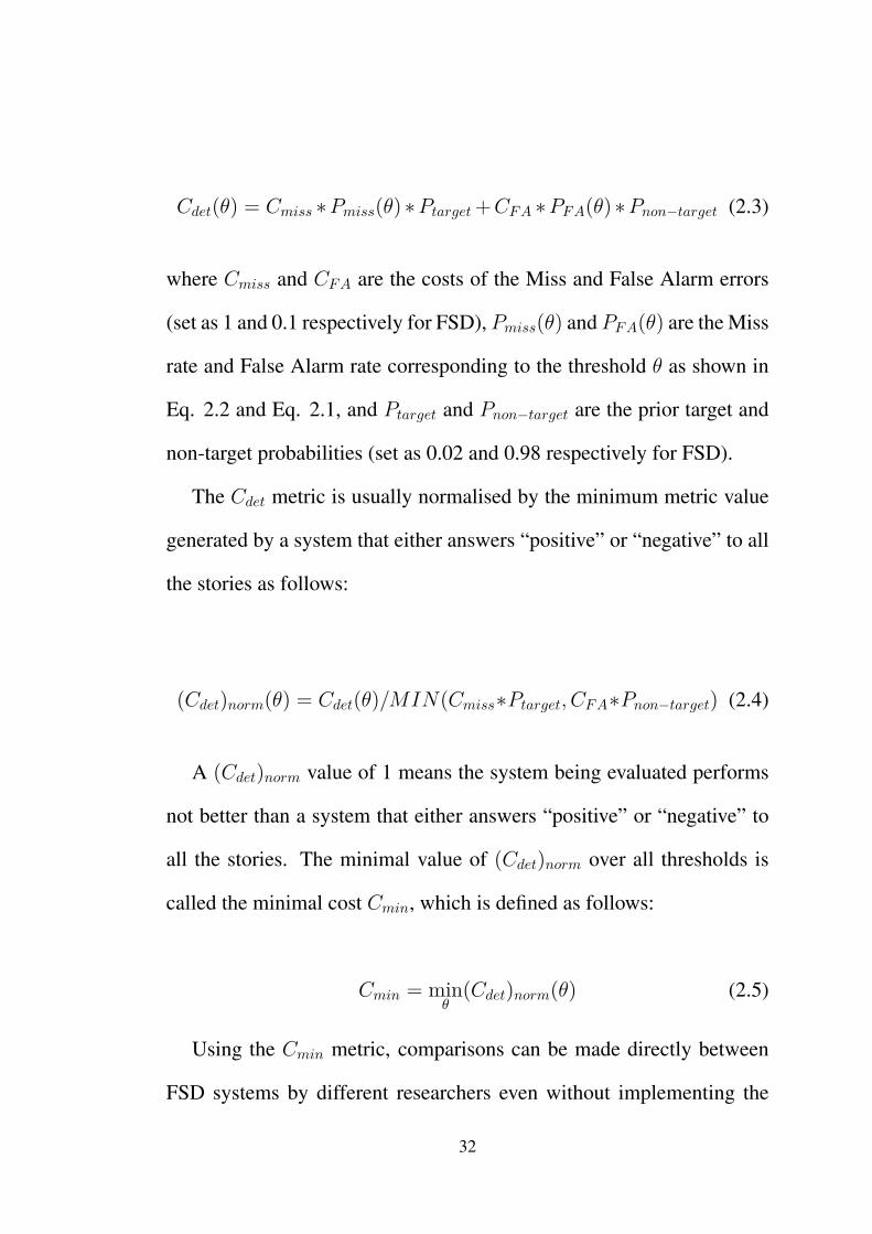
Cdet(θ) = Cmiss ∗Pmiss(θ) ∗Ptarget +CFA ∗PFA(θ) ∗Pnon−target (2.3)

where Cmiss and CFA are the costs of the Miss and False Alarm errors

(set as 1 and 0.1 respectively for FSD), Pmiss(θ) and PFA(θ) are the Miss

rate and False Alarm rate corresponding to the threshold θ as shown in

Eq. 2.2 and Eq. 2.1, and Ptarget and Pnon−target are the prior target and

non-target probabilities (set as 0.02 and 0.98 respectively for FSD).

The Cdet metric is usually normalised by the minimum metric value

generated by a system that either answers “positive” or “negative” to all

the stories as follows:

(Cdet)norm(θ) = Cdet(θ)/MIN(Cmiss∗Ptarget, CFA∗Pnon−target) (2.4)

A (Cdet)norm value of 1 means the system being evaluated performs

not better than a system that either answers “positive” or “negative” to

all the stories. The minimal value of (Cdet)norm over all thresholds is

called the minimal cost Cmin, which is defined as follows:

Cmin = minθ

(Cdet)norm(θ) (2.5)

Using the Cmin metric, comparisons can be made directly between

FSD systems by different researchers even without implementing the

32

systems, e.g., the current state-of-the-art FSD performances on the

TDT5 and Twitter corpora were reported respectively as 0.575 by Pet-

rovic et al. (2012) and 0.638 by Moran et al. (2016) with Cmin.

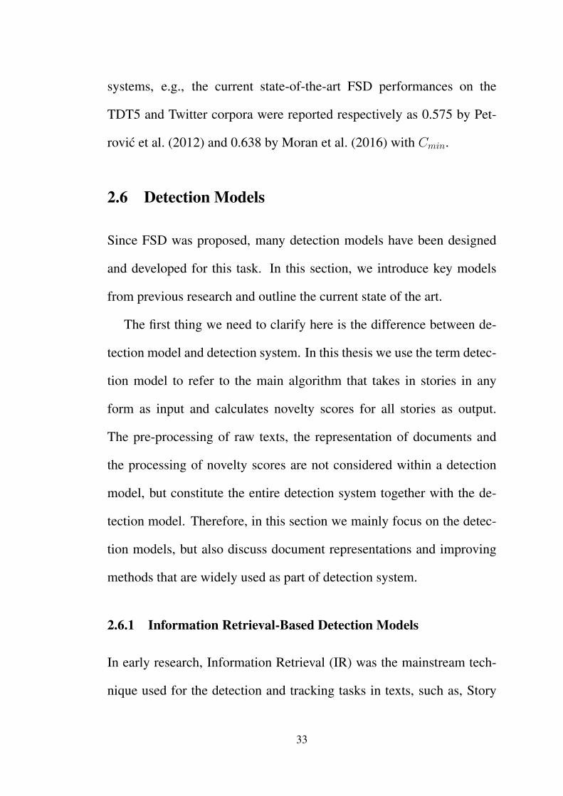
2.6 Detection Models

Since FSD was proposed, many detection models have been designed

and developed for this task. In this section, we introduce key models

from previous research and outline the current state of the art.

The first thing we need to clarify here is the difference between de-

tection model and detection system. In this thesis we use the term detec-

tion model to refer to the main algorithm that takes in stories in any

form as input and calculates novelty scores for all stories as output.

The pre-processing of raw texts, the representation of documents and

the processing of novelty scores are not considered within a detection

model, but constitute the entire detection system together with the de-

tection model. Therefore, in this section we mainly focus on the detec-

tion models, but also discuss document representations and improving

methods that are widely used as part of detection system.

2.6.1 Information Retrieval-Based Detection Models

In early research, Information Retrieval (IR) was the mainstream tech-

nique used for the detection and tracking tasks in texts, such as, Story

33

Segmentation (Ponte and Croft, 1997), Topic Detection (Willett, 1988)

and Topic Tracking (Voorhees and Harman, 1999). Typical IR problems

rely upon a user-defined query to specify what is “interesting” and find

documents that match the query. In contrast, FSD has no knowledge of

what the next new event is in the stream, so the IR-based FSD models

can only build queries based on existing stories and find the incoming

story that does not match any of the queries. The two most effective IR-

based FSD models, UMass (by the University of Massachusetts) (Allan

et al., 2000c) and CMU (by Carnegie Mellon University) (Yang et al.,

1998), are designed in this way.

UMass and CMU both tried building queries in two ways: by each

single previous story or by each centroid of previous story clusters, but

the implementation details were different from each other (Allan et al.,

1998b; Yang et al., 1998). Both systems initially adopted the single-

pass clustering algorithm to build clusters, in which, if the distance (or

dissimilarity) between the incoming story and its most similar existing

cluster (represented by the centroid of all the stories in the cluster) is

smaller than a consolidation threshold, the story is absorbed by its most

similar existing cluster; otherwise, a new cluster is generated and the in-

coming story is assigned to the new cluster as its first seed. The distance

(or mismatching) of the incoming story to the query built by its most

similar existing cluster is taken as the story’s novelty score. Although

their implementation details were different, the results of these two sys-

34

tems showed the same trend: the smaller the consolidation threshold is,

the better the FSD performance is. When the consolidation threshold is

so small that every incoming story forms a new cluster, the single-pass

clustering model becomes a nearest neighbour model, in which the nov-

elty score is defined as the distance from an incoming story to the query

built by its most similar existing story.

Given these models were based on different underlying IR systems,

UMass and CMU adopted different representations of queries and stor-

ies as well as different distance measures. Firstly, both models apply the

traditional term vector space model (Salton and Buckley, 1987) to rep-

resent queries and stories using a single element of the representation

vector for each term that occurs; though the term weights are calculated

with different weighting schemes: UMass adopted the term frequency-

inverse document frequency (TF-IDF) scheme from the INQUERY Re-

trieval system for the queries and the incoming stories (Callan et al.,

1992, 1996), while CMU, also adopted the TF-IDF representation, but

from a different IR system, SMART System (Salton, 1989), to repres-

ent both queries and stories. The weights in these weighting scheme

are initially calculated based on a background corpus such as the TREC

corpora (Harman, 1993), and remain the same in UMass (Papka et al.,

1999) but keep on being updated incrementally in CMU as the incom-

ing stories are taken into account for the calculation of inverse document

frequency in the detection (Carbonell et al., 1999). The static and dy-

35

namic properties of the TF-IDF representation will be fully discussed in

Chapter 4 and 5.

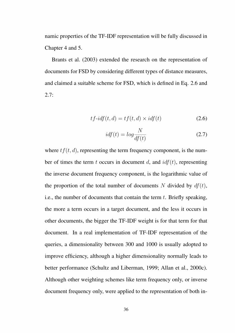
Brants et al. (2003) extended the research on the representation of

documents for FSD by considering different types of distance measures,

and claimed a suitable scheme for FSD, which is defined in Eq. 2.6 and

2.7:

tf -idf(t, d) = tf(t, d)× idf(t) (2.6)

idf(t) = logN

df(t) (2.7)

where tf(t, d), representing the term frequency component, is the num-

ber of times the term t occurs in document d, and idf(t), representing

the inverse document frequency component, is the logarithmic value of

the proportion of the total number of documents N divided by df(t),

i.e., the number of documents that contain the term t. Briefly speaking,

the more a term occurs in a target document, and the less it occurs in

other documents, the bigger the TF-IDF weight is for that term for that

document. In a real implementation of TF-IDF representation of the

queries, a dimensionality between 300 and 1000 is usually adopted to

improve efficiency, although a higher dimensionality normally leads to

better performance (Schultz and Liberman, 1999; Allan et al., 2000c).

Although other weighting schemes like term frequency only, or inverse

document frequency only, were applied to the representation of both in-

36

coming stories and queries (or only queries), they did not lead to as good

performance as TF-IDF (Allan et al., 1999).

For the measure of the distance between a query and an incoming

story, many different types of distance measures have been examined

for the FSD task, such as cosine distance, weighted sum (Turtle and

Croft, 1991), language model (Allan et al., 2000c) and KL divergence

(Lavrenko et al., 2002), and the experimental results showed that co-

sine distance outperforms other measures, especially for the TF-IDF

representation with a high dimensionality (Allan et al., 2000c), which

is defined in Eq. 2.8:

cosine_distance(~d, ~d′) = 1−~d · ~d′∣∣∣∣~d∣∣∣∣∣∣∣∣~d′∣∣∣∣ (2.8)

where ~d and ~d′ are the TF-IDF representation vectors that we are com-

paring.

As we introduced above, the TF-IDF representation in Eq. 2.6 and

2.7 and the cosine distance in Eq. 2.8 are the most effective combination

of representation and distance used in FSD (Petrovic et al., 2010b; Pet-

rovic, 2013; Moran et al., 2016), and thus, we take them as the standard

baseline approaches for FSD in this dissertation.

37

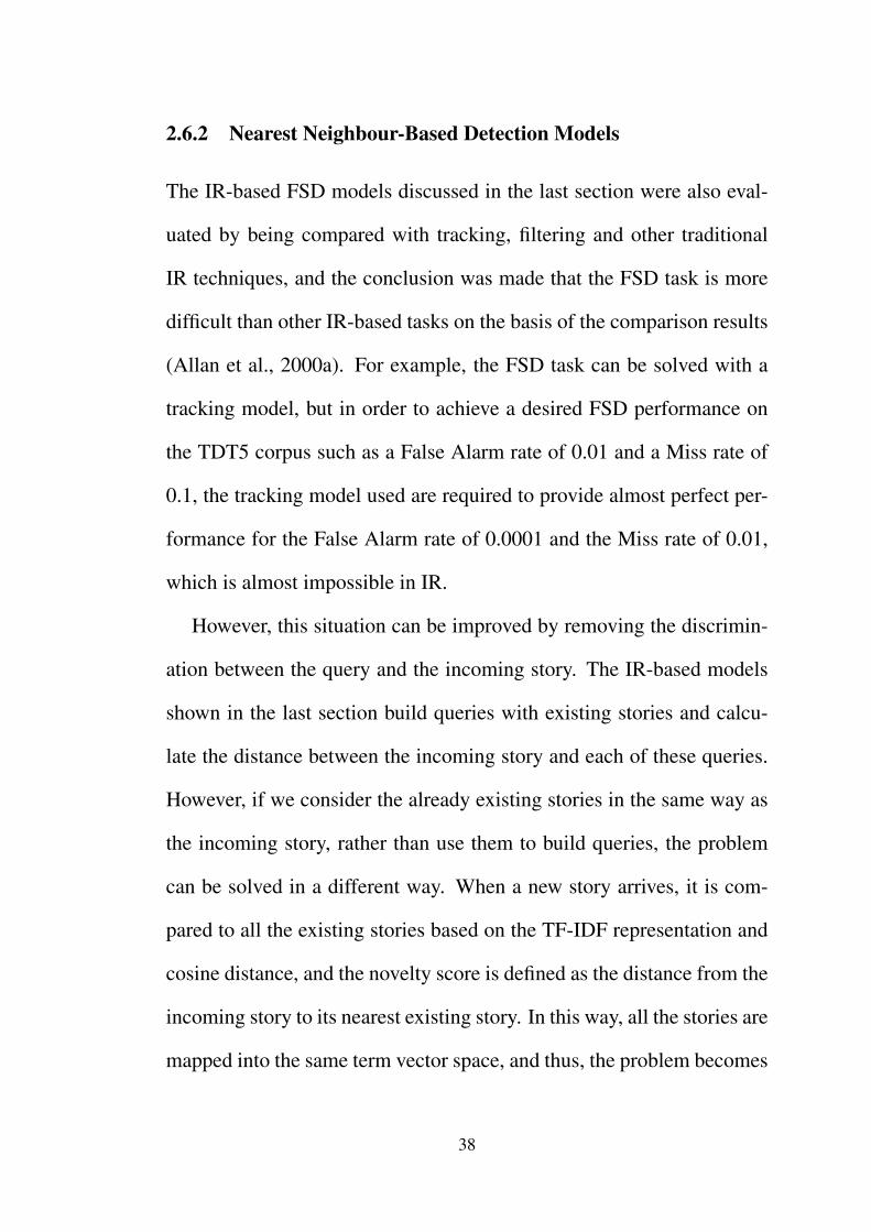
2.6.2 Nearest Neighbour-Based Detection Models

The IR-based FSD models discussed in the last section were also eval-

uated by being compared with tracking, filtering and other traditional

IR techniques, and the conclusion was made that the FSD task is more

difficult than other IR-based tasks on the basis of the comparison results

(Allan et al., 2000a). For example, the FSD task can be solved with a

tracking model, but in order to achieve a desired FSD performance on

the TDT5 corpus such as a False Alarm rate of 0.01 and a Miss rate of

0.1, the tracking model used are required to provide almost perfect per-

formance for the False Alarm rate of 0.0001 and the Miss rate of 0.01,

which is almost impossible in IR.

However, this situation can be improved by removing the discrimin-

ation between the query and the incoming story. The IR-based models

shown in the last section build queries with existing stories and calcu-

late the distance between the incoming story and each of these queries.

However, if we consider the already existing stories in the same way as

the incoming story, rather than use them to build queries, the problem

can be solved in a different way. When a new story arrives, it is com-

pared to all the existing stories based on the TF-IDF representation and

cosine distance, and the novelty score is defined as the distance from the

incoming story to its nearest existing story. In this way, all the stories are

mapped into the same term vector space, and thus, the problem becomes

38

a normal nearest neighbour problem in that space. Consequently, differ-

ent extensions for improving standard nearest neighbor models can also

be applied to FSD, and thereby improve the FSD performance.

Firstly, the normal nearest neighbour model is usually computation-

ally expensive. Because the comparisons are required to be made with

all existing stories, the calculation for each incoming story increases lin-

early as the detection process goes on, and thus becomes very inefficient

after a period. In order to solve this problem, Petrovic et al. (2010b)

considered the problem as an approximate nearest neighbour problem in

the term vector space, where the goal is to find any point that lies within

the distance of (1 + ε)r to the candidate point where ε is a very small

number and r is the distance to the nearest neighbour (Indyk and Mot-

wani, 1998). They then tried to solve this approximate nearest neighbour

problem in sublinear time using locality sensitive hashing (LSH) (Datar

et al., 2004) and finally proposed the LSH FSD model. This model

maps stories into different buckets as the stories arrive and ensures sim-

ilar stories are probably mapped into the same bucket. When a new

candidate story arrives, it is assigned to a bucket and then the search for

the (approximate) nearest neighbor is done by searching through just the

set of stories that are already in that bucket. In this way, it reduces the

processing time significantly but provides competitively good detection

performance. Thanks to this work, the FSD task can be extended to data

with much larger volume, such as social media datasets.

39

Another problem in FSD is that the high degree of lexical variation

in stories makes it very difficult to detect stories that discuss the same

event but use different words. In order to solve the kind of problem,

Petrovic et al. (2012) improved his LSH model by using paraphrases

to build a binary term-to-term matrix and applying this matrix to the

representation of stories and even the distance calculation. Although

more time and space are required in comparison to the original LSH

FSD model, this model set the state of the art of detection effectiveness

on the TDT5 corpus with aCmin of 0.575. Additionally in their research,

Petrovic et al. (2012) published the Twitter benchmark corpus for FSD,

which was introduced in Section 2.4.

Benefitting from the development of deep learning-based NLP tech-

niques, the LSH FSD with paraphrases model was extended by Moran

et al. (2016) by generating a paraphrase matrix with Word2Vec, a neural

networks model that learns distributed word embeddings by maximising

the probability of seeing specific words within a fixed context window

(Mikolov et al., 2013a,b). The paraphrases used by Petrovic et al. (2012)

are from existing lexical paraphrase sources, which only cover common

paraphrases in plain English. However, using word embeddings, Moran

et al. (2016) can automatically find good paraphrase pairs based on a

similar background corpus. This model claimed the enhancement of ef-

fectiveness of the LSH FSD model with paraphrases by approximately

9.5%, and pushed the state of the art on the Twitter target corpus to a

40

Cmin of 0.638.

It is worth noting that although the LSH FSD model by Petrovic et al.

(2012) has been considered the state of the art by by much of the sub-

sequent research on the topic (Qiu et al., 2015; Qin et al., 2017; Kannan

et al., 2018b), it is not possible to reproduce the LSH-based FSD now

because of the lack of algorithm details (Wurzer et al., 2015; Kannan

et al., 2018a; Qiu et al., 2016). We tried to reimplement the algorithm,

but could not achieve the same detection results as presented in the ori-

ginal papers, specifically because it is not clear what features are used

for building the LSH model and implementing the detection. Even so,

we still take the LSH FSD model as the state of the art to make compar-

isons with our experimental results.

2.6.3 Other General Detection Models

In addition to the (approximate) nearest neighbour-based FSD models,

there have been a number of different types of models proposed for the

FSD task.

The Dragon System (Allan et al., 1998a) built story and cluster rep-

resentations with only single term frequencies, and added a pre-process-

ing step in which a k-means clustering was used to build 100 background

clusters from a background corpus. In the detection process, a story is

considered to be discussing a new event when it is closer to a background

cluster than to an existing story cluster.

41

Stokes and Carthy (2001) investigated if the FSD performance can

be improved by taking into account both semantic (using lexical chain)

and syntactic (using proper nouns) information. However, their results

showed that only a marginal increase in system effectiveness is achieved.

Zhang et al. (2005) and Ahmed et al. (2011) used probabilistic mod-

els, specifically those based on non-parametric Bayesian approaches, to

handle an increasing number of clusters, and model the uncertainty to

match the story with clusters. However, they were computationally ex-

pensive and lagged behind non-probabilistic models in terms of effect-

iveness.

Osborne et al. (2012) evaluated whether Wikipedia can be used to im-

prove the detection performance by blocking spurious events. Their res-

ults showed that although it is a powerful filtering mechanism for mean-

ingful events, Wikipedia usually lags behind other medias, and thus has

limited usefulness in real-time event detection.

Wurzer et al. (2015) designed a new detection model for FSD, k-

term hashing, in which the incoming story is compared to a look-up

table that contains all the combinations of up-to-k terms occurring in

any existing story. This model was extended recently by assigning dif-

ferent weights to the term combinations with different characteristics,

and achieved good performance (Wurzer and Qin, 2018).

Some more traditional novelty detection models can also be applied

in an online style for FSD; these include the autoencoder and one class

42

classification models. An autoencoder (Thompson et al., 2002; Vincent

et al., 2008) is a neural network-based model which is trained to recon-

struct the input data on the output side but which is designed such that

the input data must pass through a representational bottleneck (often a

hidden layer with a smaller number of neurons than the input and outputs

layers) thereby ensuring that the autoencoder is not simply a copy func-

tion (Kelleher, 2019). Autoencoders are often used to generate low di-

mensional representations of inputs, by using the representations learned

at hidden layer to represent an input vector. In these scenarios the nov-

elty or dissimilarity of an input relative to existing data points is calcu-

lated in this lower dimensional feature space. Another way of using au-

thoencoders for FSD is to measure novelty in terms of the reconstruction

loss for an autoencoder for an input vector: the more similar an input is

to the data the autoencoder was trained on the lower the reconstruction

loss will be, and vice versa. The adversarial autoencoder (Makhzani

et al., 2015) is a variant of the autoencoder model that is inspired by

generative adversarial nets (GAN) (Goodfellow et al., 2014) and adds

distributional limitation onto the low-dimensional features. Using an

adversarial autoencoder model, Leveau and Joly (2017) built a recon-

struction model with all the existing stories, and input the new story

into the model. The mean square error (Chou and Juang, 2003) between

the input and output are taken as the novelty score. Additionally, many

novelty detection application can be solved as a one class classification

43

problem, where an overall model is built based on all existing data and

the output of the model for the incoming data is taken as the novelty

score. For example, the one class SVM model (Schölkopf et al., 2001;

Tax and Duin, 2004) generated a hyper-sphere based on all existing data,

and the distance of each incoming data points to the hyper-sphere was

considered to be the novelty score. However, both the autoencoder and

one class classification models lead to high computational complexity,

while their effectiveness has not been compared with other models.

2.6.4 Detection Models for Specific Purposes

All the FSD models that have been discussed to this point are general

detection models that are designed for stories in plain English and can

be applied to different corpora and application areas. However, there

are also some other FSD models designed especially for some specific

application situations.

Braun and Kaneshiro (2003) and Kumaran and Allan (2005) integ-

rated binary supervised classifiers to decide whether an incoming story

discusses a new event. Both models train the classifiers with previous

TDT corpora and test with the TDT5 corpus. Prior knowledge from the

training sets is also exploited in detection, e.g., the location features by

Braun and Kaneshiro (2003) and the topic terms by Kumaran and Allan

(2005). Although they achieved the highest evaluation score for TDT5

at that time, these supervised models are difficult to extend to other cor-

44

pora due to the limitation of insufficient training data.

Some other research works only explore FSD on the events in some

specific areas, e.g., the model proposed by Kannan et al. (2018a,b) used

prior knowledge of sport to detect only events in Cricket, and thus are

not within our research focus.

In recent years, in response to the growth of user generated content

(UGC) and social media, a number of FSD systems have been developed

that are specifically designed for social network data such as Twitter

(Li et al., 2012; Thurman et al., 2016; Zhang et al., 2017). Especially,

Qiu et al. (2015) proposed the Nugget-based model for FSD in Twitter,

which takes advantage of special properties of Twitter data like the “@”

and hashtag, and uses them to build the “nuggets” of events. When a

new tweet arrives, it only needs to be compared with these event nug-

gets rather than the tweets in events to make a decision. Using this

approach, Qiu et al. (2016) claimed very good performance with a Cmin

of only 0.280. However, as we mentioned in Section 2.3, our research

focuses on generalisable FSD systems, so the results of this specifically-

for-Twitter model is not taken into account as the state of the art.

2.6.5 Improving Methods

In addition to different detection models, there are many other methods

that have been designed for FSD to improve the detection performance.

From the very beginning of research on FSD, it was noticed that the

45

stories discussing the same event tend to be temporally focused, and a

time gap between bursts of topically similar stories is often an indication

of different events (Yang et al., 1998). This knowledge has been taken

advantage of in two ways: 1) discounting the distance of the incoming

story to the existing stories that arrived long ago or raising the novelty

threshold for the novelty scores generated by very old existing stories

(Allan et al., 1998b; Yang et al., 1998; Qin et al., 2017); and 2) Lim-

iting the nearest neighbour to the stories within a time window so that

old stories are excluded (Yang et al., 1998; Luo et al., 2007; Petrovic

et al., 2010b; Qiu et al., 2016), which is also a method commonly used

in online novelty detection (Zhang et al., 2008; Gupta et al., 2013). Both

methods improve the detection performance of original models. How-

ever, the first method brings in extra computations, while the second

method significantly reduces the computations, and therefore, the time-

sensitive method with a time window has become a standard method for

improving FSD.

An event can be considered to be the integration of “who”, “when”,

“where”, “what” and “how” (Papka and Allan, 2002). From this aspect,

named entities are intuitively considered to be helpful for FSD. How-

ever, in real use, the highlighting of named entities either makes only

slight improvement that can be ignored (Allan et al., 1999; Panagiotou

et al., 2016; Rao et al., 2017), or limits the model to some specific pur-

poses (Yang et al., 2002; Kumaran and Allan, 2004; Zhang et al., 2007;

46

Zhao et al., 2017; Li et al., 2017), and thus is usually not adopted in

general FSD.

In terms of the methods of stemming and removing stopwords, which

are issues for almost all NLP tasks, Allan et al. (1999) made compre-

hensive evaluation and provided credible results: stemming and remov-

ing stopwords can only slightly improve the detection performance; but

are still recommended for FSD for the sake of improving detection effi-

ciency. Consequently, the vast majority of subsequent research followed

this trend, including the state-of-the-art systems for both the TDT5 and

Twitter corpora (Petrovic et al., 2012; Moran et al., 2016).

2.7 Discussion

Based on the research introduced in this chapter, we can see that a vari-

ety of solutions have been proposed for the FSD task. However, the vast

majority of this research tends to apply different types of models and

methods to get better performance, but few focus on an analysis of the

reason for which a model or method might improve or harm the detec-

tion. There are also many open questions relating to the FSD task that

need to be answered: firstly, almost all the previous research detects first

stories based on the occurrences of different terms, but it is not clear that

this is the only way for people to make the decision, e.g., “a dog bites

a man” and “a man bites a dog” include the same terms but obviously

47

describe two different events, and the latter is more likely to be an inter-

esting event for people; secondly, it has been shown that the distance to a

single existing story can represent the novelty of a new story better than

the distance to a cluster of existing stories, but it is not clear why this is

the case; thirdly, most of previous research adopts the TF-IDF document

representation, but the details of how the TF-IDF models work for the

comparison between the incoming story and an existing story have not

been well discussed yet. All of these questions can be aggregated into

one research question for FSD: what is the most crucial factor in defin-

ing “story novelty”. To make progress on the FSD task, we argue that a

multi-dimensional analysis of this question is needed.

2.8 Summary

In this chapter, we started from the introduction of online novelty de-

tection and the TDT project series, the two sources where the FSD task

originated from, and then gave definitions for the basic concepts in the

task. After that, we presented the corpora specifically designed for the

FSD task, as well as the evaluation methods used in this research. We

also summarised the detection models for FSD based on IR-based mod-

els, nearest neighbour-based models, other general models, and models

for specific purposes; and went on to introduce some useful methods for

improving FSD. Finally, we stated the most important research problem

48

for FSD - it is still not clear what is the most crucial factor in defining

the “story novelty”.

This chapter outlines the current situation of the research on FSD,

and from the next chapter, we will start our three dimensional analysis

of the problem from the perspectives of distance, time and terms.

49

Chapter 3

Detection Model Categorisation and

Analysis

As discussed in the previous chapters, we believe that the most import-

ant research problem to be solved in this research is the question of

what is the most crucial factor in defining the “story novelty”. We also

argue that the clear exposition of the definition of novelty is the basis

of designing a proper detection model and enhancing its performance.

In our specific research area, the novelty score of each story plays the

role of the definition of novelty. The way to calculate the novelty score

varies in different detection models, which means that different models

effectively adopt different ways to define the story novelty.

To explore these issues further, in this chapter, we firstly identify

three main categories of detection models based on different types of

distances in the definition of novelty scores, and then verify the per-

formances of different categories of models with different document

50

representations, and try to find out the potential reasons that underlie

the performances of different models and document representations.

We organise the structure of the chapter as follow: we start from

our proposed categorisation method and the introduction to the three

categories of models in Section 3.1, followed by the empirical compar-

isons across these categories of models in Section 3.2. In Section 3.3,

we evaluate the performances of different types of document representa-

tions in each category of models, and then analyse the potential reasons

that may cause the different performances in Section 3.4. We summar-

ises in Section 3.5.

3.1 Three Categories of Detection Models

To date there is no systematic categorisation method for FSD detection

models. Only in the much broader research area, has there been a gen-

eral categorisation of novelty detection models proposed by Pimentel

et al. (2014), which included: probabilistic, distance-based, reconstruct-

ion-based, domain-based, and information-theoretic models. However,

this categorisation is established solely on the techniques used in the

detection model, and therefore does not naturally provide comparisons

across the categories, nor insights into how the different categories of

models define the concept of novelty.

In order to frame definitions of novelty in FSD, we propose (based on

51

our analysis of the FSD literature in Chapter 2) three categories of nov-

elty scores, and, three corresponding categories of FSD models, these

are: Point-to-Point (P2P) models, Point-to-Cluster (P2C) models, and

Point-to-All (P2A) models. This categorisation is based on different

distances used to define novelty scores in different models. The concept

of distance we are using here is a general expression that refers to the

difference or dissimilarity between two objects, which can be two stor-

ies, a story and a cluster, or a story and all other stories. Within these

three categories any mathematical definition of distance (e.g., cosine,

Euclidean, etc.) is usable, with the selection typically driven by the em-

pirical performance of the model. The three categories of models are

detailed as follows:

Point-to-Point (P2P) models, in which the novelty score is defined as

the distance from the incoming candidate story to an existing story:

Novelty_ScoreP2Pdef= distance(storynew, storyexisting) (3.1)

The nearest neighbour-based model is a typical example of a P2P

FSD model, in which the novelty score is defined as the distance from

the incoming story to the closest existing story to it. In order to improve

efficiency, P2P models usually accept an approximate nearest neighbour

to each candidate story, instead of the true nearest neighbour. For ex-

52

ample, the CMU model (Yang et al., 1998) only seeks the nearest neigh-

bour in the latest 2,000 stories; and, the LSH FSD model (Petrovic et al.,

2012; Moran et al., 2016), which achieves the state of the art in FSD,

allocates existing stories into a number of buckets and only seeks the

nearest neighbour in the bucket that the new story is assigned to. The dis-

tance between two stories could be in different forms, and as explained

in Section 2.6, cosine distance is usually a good option for FSD.

Point-to-Cluster (P2C) models, in which the novelty score is defined

as the distance from the incoming candidate data to a cluster of existing

stories:

Novelty_ScoreP2Cdef= distance(storynew, clusterexisting) (3.2)

Different from that in P2P models, the distance in defining the nov-

elty score in P2C models is between the incoming story and a sub-space

(or the union of sub-spaces) formed by a cluster of existing stories in

the feature space. In the calculation, the distance could be the distance

to a representative of the subspace, the distance to the range of the sub-

space, or even the distance to the output of a model trained by the cluster

of stories in the sub-space. In the context of FSD, a cluster can be in-

tuitively understood as a topic behind the texts. To make it simple, the

cluster is usually represented by some point within its range, e.g., the

53

centroid of the cluster, the furthest point or the closest point to the new

data point, and in this case, the P2C distance is simplified into a P2P

distance. The UMass and CMU clustering models (Allan et al., 2000c;

Yang et al., 1998) are both based on the single-pass clustering, which

is a typical P2C model based on the distance from the new story to the

centroid of the closest cluster to it.

Point-to-All (P2A) models, in which the novelty score is defined as the

distance from the incoming candidate story to all the existing stories:

Novelty_ScoreP2Adef= distance(storynew, all_storiesexisting)

(3.3)

Given all existing data, the detection of novelty can be considered

as a one class classification problem, in which the quantity of existing

normal data is large enough to build the “normality”, but the quantity

of abnormal data is insufficient to build the novelty class for classifica-

tion. One class SVM (Schölkopf et al., 2001) is a popular model in one

class classification, the basic idea of which is to generate a hyper-sphere

based on all existing data, and all the data outside the hyper-sphere are

considered to be novel data.

It is worth highlighting that any novelty detection model that is based

on a machine learning model trained on all the existing data can be

viewed as a type of P2A model. For example, the k-term hashing model

54

(Wurzer et al., 2015; Wurzer and Qin, 2018) compares all the combin-

ations of up-to-k terms in the incoming candidate story with a look-up

table created using all existing stories, and takes the proportion of new

combinations as the novelty score, and so it can be considered a P2A

model. Furthermore, there is a type of model, specific to novelty de-

tection, the reconstruction-based models (Pimentel et al., 2014), which

seems to be a class of Point-to-Itself models but are actually P2A mod-

els. For example, when an autoencoder (Leveau and Joly, 2017) is ap-

plied for FSD, the novelty score of an incoming candidate story is cal-

culated as the degree of reconstruction of itself through the autoencoder

neural network architecture. This is also a P2A model because the au-

toencoder architecture is trained with all the existing stories.

From these definitions, we can understand the relationships among

these three model groupings. When the clusters in a P2C model are

very small, the model can be approximately considered as equivalent

to a P2P model, with each data point (and a limited sub-space around

it) as a cluster. In contrast, when the cluster in a P2C model is big

enough to contain all the data points, the model becomes equivalent to

a P2A model. From this perspective, P2C is the general model form for

defining novelty scores, and P2P and P2A are special cases of P2C with

specific cluster size. As the detection of a first story always requires the

comparison between the candidate story and some cluster of existing

55

stories, any detection model can be categorised into one of these three

types of models, or any combination of them, e.g., our proposed method,

the New Term Rate (NTR) method, is a P2A or P2C method that can be

used with the combination of almost any other model.

Based on the descriptions given above, we can see that the differ-

ences between these three categories of models are actually dependent

on the target object from which the distance of the candidate story is

defined, rather than what domain theories and/or model architectures

are used. Using these three categories of models, we can analyse not

only the performance of a single detection model, but also the common

characteristics of models within a category, and furthermore, perform

cross category comparisons based on these general characteristics. As

a practical example of this we can compare the performances of FSD

in different document representations, and obtain deeper insights into

both the concept of story novelty and the appropriateness of particular

document representations. We now turn to this task.

3.2 Comparisons across Different Categories

In this section, we make comparisons across different categories of FSD

models in the standard benchmark corpus, TDT5, which was introduced

in Section 2.4. To do so, we select a typical model for each category of

our proposed classes, and apply them to FSD on the TDT5 corpus.

56

3.2.1 Experimental Design

For this experiment, in order to reduce the effect of useless terms and

different term forms, for all story texts we remove terms with very high

and very low document frequency (stopwords and typos), and stem all

terms into their roots using the Krovetz stemmer (Krovetz, 2000). This

text pre-processing method is implemented for all experiments in this

and all the following chapters. After that, all the stories are mapped

into the term vector space with the TF-IDF weighting scheme defined

in Eq. 2.6 and 2.7; thus the detection and analysis for the experiment in

this section are carried out with only the TF-IDF document representa-

tion. To improve efficiency, we limit the dimensionality of the TF-IDF

representation to 10,000.

For P2P, we adopt the traditional nearest neighbor model as the rep-

resentative model. The incoming story is compared to all existing stor-

ies to find the nearest neighbour. If the distance to the nearest neighbour

exceeds a threshold, the story is declared novel. Our implementation

adopts the cosine distance in Eq. 2.8, and only makes comparisons with

the 2,000 most recent existing stories, which are the stories within a time

window of approximate 30 hours in TDT5, the same as the time window

method used by Yang et al. (1998).

The P2C category is represented by a single pass clustering model

just like in the UMass and CMU clustering models (Allan et al., 2000c;

57

Yang et al., 1998). As discussed in the introduction of P2C, the clusters

represent topics behind the texts, and each cluster can be represented

by its centroid, which is calculated as the mean of the vector repres-

entations of the stories in that cluster. Similarly, the incoming story is

compared to the centroids of all the clusters to find the nearest cluster. If

the distance to the nearest cluster does not exceed a threshold, the story

is declared non-novel and assigned to the nearest cluster after which the

cluster centroid is updated; otherwise, we declare the story novel, and

create a new cluster with this new story as the only data point within the

cluster, and therefore, also the centroid. The fact that clusters are rep-

resented by centroids means that, once the cluster has been selected, the

calculation of distance within the P2C model is, essentially, transformed

into a P2P distance, so the cosine distance is also adopted in calculating

the distance from the new story to a cluster.

For P2A, we select a one class SVM model (Schölkopf et al., 2001)

as the representative model because using this model makes it easy to

interpret the distance from a story to all existing stories. Given a para-

meter V between 0 and 1, all data are mapped into a hyper-space using

a kernel function to generate a sphere that contains 1-V of the data in-

side it as normal data and V of the data outside it as novel data. In our

model, we do not take the label by the one class SVM model as the label

of novelty for a candidate story, but take the distance of the story to the

sphere as the novelty score, with a positive value if the data is outside

58

the sphere and negative value if the data inside it. Finally, to reduce the

computational cost associated with repeatedly rebuilding the one class

SVM, for each new story we only use the 2,000 most recent data points

to build the model.

3.2.2 Experimental Results

We present our evaluation in terms of DET curves and AUC scores as

introduced in Section 2.5. Because we attempt to only make analysis

across different categories of models rather than find the best threshold

or compare with results from other researchers, we do not need to set

Cmin in this evaluation.

Specifically for the one class SVM model (for the P2A class), we

implement a number of validation tests for the selection of parameters

and representation dimensionalities, and based on the validation results,

we select 0.1 as the value of V in this part of experiment, and limit

ourselves to a dimensionality of 1,000 for the TF-IDF representation.

The DET curves, shown in Figure 3.1, demonstrate that there is a

general trend that the performance gets worse as we move from P2P to

P2C and P2A, which is also clearly shown by the AUC scores of the

DET curves: 0.1094, 0.1441 and 0.2531 for P2P, P2C and P2A models

respectively.

These results also correspond with the results claimed in previous

FSD research that the performance of the single pass clustering gets

59

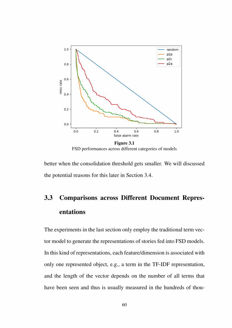
Figure 3.1FSD performances across different categories of models

better when the consolidation threshold gets smaller. We will discussed

the potential reasons for this later in Section 3.4.

3.3 Comparisons across Different Document Repres-

entations

The experiments in the last section only employ the traditional term vec-

tor model to generate the representations of stories fed into FSD models.

In this kind of representations, each feature/dimension is associated with

only one represented object, e.g., a term in the TF-IDF representation,

and the length of the vector depends on the number of all terms that

have been seen and thus is usually measured in the hundreds of thou-

60

sands. Therefore, for a representation of the story with hundreds or less

of terms, only the features that represent terms existing in the story are

set as non-zero values and all the other features are set as zero. Thus

the term vector document representations are usually sparse features. In

recent years a large number of deep learning-derived distributed doc-

ument representations have been proposed and achieved excellent per-

formance across many NLP tasks (Goldberg, 2017). Unlike the tradi-

tional term vector representations that capture one term independently

with one feature, distributed representations always represent each ob-

ject with multiple representational features, and each feature is associ-

ated with more than one represented object. Instead of representing ob-

jects, the features represent abstract characteristics of objects rather than

objects themselves. Therefore, distributed representations are usually

dense features with only a few hundred dimensions. In this section, we

first introduce different types of distributed document representations,

and then make comparisons to traditional term vector representations in

different categories of FSD models.

3.3.1 Distributed Document Representations

Distributed representations have been explored in NLP for many years

(Hinton et al., 1984), but have become the predominant document rep-

resentations in NLP recently due to the facilitation of deep learning

(LeCun et al., 2015). Specifically there are mainly two types of deep

61

learning-based distributed document representations based on the ways

they are generated:

Accumulated word embeddings, is the simple accumulation of the

word representations (or word embeddings) of all the words in the docu-

ment. Word embeddings attracted research attentions earlier than docu-

ment representations. Mikolov et al. (2013a,b) proposed the Word2Vec

word embeddings in 2013, the generation of which is based on two lan-

guage models with shallow neural network architectures: CBOW (con-

tinuous bag of words) and Skip-gram. The CBOW model takes the sur-

rounding words in a context as input to predict the central word in the

output side, while Skip-gram uses only the central word as input and

attempts to predict all its surrounding words.

The Word2Vec embeddings have been proved to be powerful and

have many properties that were never achieved by the research before

it, e.g., operations can be made between the Word2Vec embeddings

like vector(′′King′′)− vector(′′Man′′) + vector(′′Woman′′) ≈ vector

(′′Queen′′). Because they are trained on large unlabelled corpora, Word-

2Vec embeddings can be applied in a generalised way for many NLP

tasks. One limitation of Word2Vec embeddings is that a distinct vector

representation is assigned to each word, so it can not handle the out-

of-vocabulary (OOV) words (i.e., the words that did not appear in the

training data). In order to deal with this problem, Bojanowski et al.

62

(2017) proposed the FastText model, which is based on the Skip-gram

model but uses a bag of character n-grams to represent a word. Us-

ing the morphology of words, FastText can generate word embeddings

for the OOV words by finding the already-known n-grams in the OOV

words. It is very important to handle the OOV words for some spe-

cific tasks just like FSD, where the whole corpus is always unavailable.

Both Word2Vec and FastText are static word embedding models that

represent each word with a fixed vector. Very recently, Peters et al.

(2018) proposed a dynamic word embedding model, ELMo (Embed-

dings from Language Models), in which different word embeddings are

generated for the same word according to different contexts around the

word. This model is based on a multi-layer bidirectional sequential lan-

guage model, which takes the sentence as input. Each layer outputs

a context-dependent representation, and representations from different

layers represent different characteristics of word use, e.g., syntax and

semantics. The final word embedding output by the ELMo model is the

combination of representations from different layers, and thus, it is not

only context-dependent, but also integrates different characteristics of

word use.

Given these word embeddings, the document representation can be

calculated by accumulating the word embeddings of all the words in the

document, e.g., averaging, concatenation or summing. The averaged

word embeddings have been shown to be an effective document repres-

63

entation in many NLP tasks (Wieting et al., 2015; Arora et al., 2016).

Directly-generated document representations, are representations ge-

nerated directly from the neural networks for each document, rather than

the accumulation of word embeddings. The first well-known document

representation model of this kind is the Paragraph Vector proposed by

Le and Mikolov (2014), which follows the architectures of Word2Vec

but embeds a new input to train the document representation at the same

time. In this way, the Paragraph Vector can learn fixed-length docu-

ment representations from variable-length texts, regardless of whether

they are sentences or paragraphs. Some other models, also in an unsu-

pervised way, were however proposed only for sentences. Skip-thought

(Kiros et al., 2015), as well as its variants, Quick-thoughts (Logeswaran

and Lee, 2018) and FastSent (Hill et al., 2016), adopt the ideas from

Skip-gram, but use the central sentence to predict the surrounding sen-

tences. This training process is based on the order and inner relations of

sentences, therefore is not suitable for stories in FSD that are documents

independent of each other.

Although unsupervised learning is intuitively considered the way to

generate document representations for general use, supervised learn-

ing can also be applied to this purpose. Conneau et al. (2017) adop-

ted the Stanford Natural Language Inference corpus (Bowman et al.,

2015) to generate document representations from the task of Natural

64

Language Inference (NLI). The results showed that the document rep-

resentations trained for the NLI task can be transferred to many other

NLP tasks and achieve even better performance than the unsupervised

document representations like Paragraph Vector and Skip-thought. Sub-

sequently, Subramanian et al. (2018) extended the research of Conneau

et al. (2017), and trained the general document representation in su-

pervised learning with multiple tasks in NLP such as Neural Machine

Translation, Constituency Parsing and NLI. The very recent model pro-

posed by Devlin et al. (2018), BERT (Bidirectional Encoder Repres-

entations from Transformers), adopted the attention-based transformer

architecture (Vaswani et al., 2017) and combined unsupervised and su-

pervised learning tasks during training. The document representations

generated by BERT created the state of the art for a wide range of tasks,

such as question answering and NLI.

It is worth noting that the order of terms in a document is taken into

account in the generation of distributed representations. This is true irre-

spective of whether a sliding window, recurrent architecture or attention-

based architecture are used. Consequently, using a distributed represent-

ation generated by any of these methods “a dog bites a man” and “a man

bites a dog”, the examples used in Section 2.7, will have different rep-

resentations so that the distinction between the two events can be made

and so (assuming a normal story history) it is possible for the detection

65

model to find the latter to be a new event that has not happened before.

However, the distinction between these two stories would be lost using

a term vector model and so these models would not be able to identify

the novelty of one story in the context of the other.

Additionally, many of these distributed document representations ha-

ve pre-trained models published for general use, such as Word2Vec,

FastText and BERT. These models are normally pre-trained with a very

large scale of data so that they can be transferred well to other tasks,

e.g., Word2Vec is trained on roughly 100 billion words from a Google

News dataset. In Section 3.3.2, we adopt one typical distributed docu-

ment representation from each type, and empirically compare them with

the traditional TF-IDF representation for the FSD task. To the best of

our knowledge, our published paper in this work was the first research to

apply deep learning-based distributed document representations to this

specific task.

3.3.2 Experiments

For the comparisons between the TF-IDF representation and distributed

representations for the FSD task, we implement experiments in all three

categories of detection models. The typical model selected for each cat-

egory, the setting for the detection models and the implementation of

the TF-IDF representation are exactly the same as in Section 3.2. For

the distributed representations, we also selected one typical representa-

66

tion from each type, i.e., Word2Vec for accumulated word embeddings

and BERT for directly-generated document representations. For both

selected document representations, we adopt their published pre-trained

models rather than train them with any specific dataset, which is also for

the generalisation of our research results. Finally, the dimensionalities

of the Word2Vec and BERT document representations used in this ex-

periment are 300 and 768 respectively, which are of course much smaller

than the dimensionality of the TF-IDF representations.

The comparison of results are presented in Fig. 3.2, 3.3 and 3.4 re-

spectively, one for each category of models. Within each figure three

DET curves are plotted, one for each document representation: TF-IDF,

Word2Vec, and BERT. The corresponding AUC scores of all these DET

curves are shown in Table 3.1. Comparing the performances of the mod-

els across different document representations, the most important find-

ing is that for all three categories of models, the TF-IDF representation

outperforms distributed representations, and the accumulated word em-

beddings outperform directly-generated document representations. In-

deed, the performance of the models with BERT document representa-

tion is similar to random selection.

These results are somewhat surprising because the distributed docu-

ment representations, especially the BERT representation, have achieved

excellent performance in a wide range of NLP tasks. However, they in-

deed correspond with the results from previous research works that the

67

(a) P2P

Figure 3.2FSD performances across different document representations for P2P models

(a) P2C

Figure 3.3FSD performances across different document representations for P2C models

68

(a) P2A

Figure 3.4FSD performances across different document representations for P2A models

Table 3.1AUC scores across different document representations

in different categories of models

Document RepresentationsTF-IDF Word2Vec BERT

Categoriesof Models

P2P 0.1094 0.1473 0.4827P2C 0.1441 0.2255 0.4970P2A 0.2531 0.2788 0.4971

nearest neighbour-based model with the TF-IDF representation is the

state-of-the-art detection system for FSD. In the next section, we will

analyse the potential reasons and try to explain why these results hap-

pen.

69

3.4 Discussion

In terms of explaining why the performance becomes worse from P2P

to P2C and P2A, or from TF-IDF to Word2Vec and BERT, we claim one

potential reason could be that the specificity of a word in the calculation

of story novelty is diluted in a large number of documents or in the

distributed representations, which is an important loss of information

for novelty detection.

Our experimental results provide support for this hypothesis. For ex-

ample, for the event “Sweden rejected the euro”, the P2P model with the

TF-IDF representation finds the first story easily, but the P2C model, the

P2A model or the P2P model with distributed representations usually

fail because the first story is considered to be very similar to a previous

document that discusses another event “Portugal and the euro”. Firstly,

these two topics are within the same general topic, “monetary policy”,

and of course have many common terms. In the P2C and P2A models, as

a cluster of existing stories are taken as a whole in the comparisons, the

terms that indicate the difference like “Sweden” and “Portugal” are pos-

sibly contained by other irrelevant stories in the cluster, and thereby lose

their function for disentanglement. However, in story-to-story comparis-

ons in the P2P models, these terms can be effective indicators and make

stories from these two events distinguishable. Secondly, “Sweden” and

“Portugal” are two different words in the TF-IDF representations, how-

70

ever, in the Word2Vec representations, the words with common contexts

are located in close proximity to one another, that is, the two words make

little difference. Not to mention in the directly-generated document rep-

resentations like BERT, there is no explicit representation of words that

can be found. Consequently, the events in Sweden and Portugal can be

clearly distinguished from each other within the TF-IDF representation,

but it is difficult to find the novelty caused by the specificity of a word

in the distributed representations.

This, of course, is only a working hypothesis on the reason why the

P2P or nearest neighbour model with the TF-IDF representation outper-

forms other detection systems. Further research on the specificity of

a word in the calculation of story novelty requires detailed analysis on

how this detection system works for the FSD task.

On the other hand, we can see that the fact that a distributed docu-

ment representation is able to represent the order of words in a document

does not appear to be of significant benefit for the FSD task. This may

be because the specificity of words plays a more important role in FSD

than the order of terms, but it can also be because most of the events in

the TDT5 corpus happen to be about new things, rather than about old

things with new activities. In order to take advantage of both the spe-

cificity and the order of terms, the combination of different types of rep-

resentations might be a useful approach to improve model performance.

To test this we implemented extra experiments using the concatenation

71

of TF-IDF and distributed document representations, but the results of

these experiments showed little improvement on the results for models

using only the TF-IDF representations. We will design and test more

ways of combination of representations in the future work.

3.5 Summary

In this chapter, we firstly proposed a new categorisation method for FSD

models based on different distances in the definition of novelty, and then

implemented experiments to make comparisons across different categor-

ies of models with different document representations. From this we

observed that the nearest neighbour-based models with TF-IDF repres-

entation outperform other FSD systems, and found that one potential

reason for this could be that the specificity of a word in the calcula-

tion of story novelty is diluted in a large number of documents or in the

distributed representations. In order to make further analysis on this hy-

pothesis, we will look into the details of how the detection is processed

in the nearest neighbour model with the TF-IDF representation in the

next two chapters, and attempt to find the most crucial factor in defining

the story novelty.

72

Chapter 4

Background Corpus Selection and

Evaluation

As shown in previous research in Chapter 2 and our discussions of mod-

els and document representations in Chapter 3, the nearest neighbour

model with the TF-IDF representation outperforms other FSD systems,

and the potential reason might be that it preserves the specificity of a

word in the calculation of story novelty better than other systems. How-

ever, in order to deepen the research on this point, it is required to

look into the details of how this system operates for FSD. Motivated

by this, in this chapter we investigate the nearest neighbour model for

the FSD task with representations generated by the basic TF-IDF model,

the static TF-IDF model, which applies fixed vocabulary and IDF values

throughout the detection process, and analyse some key factors in the

static TF-IDF models that affect the performance of FSD, with respect

to terms and the corpora where the terms are from.

73

The majority of machine learning research assumes that the data gen-

eration process is stationary, i.e., the data used for building a model

and making inference are sampled from the same distribution. How-

ever, because of its online characteristic, one challenge faced by FSD

systems is that the system’s vocabulary (and hence document repres-

entation) cannot be derived from a target corpus, but must instead be

defined by the vocabulary of a background corpus. The resultant poten-

tial difference between the background and target corpora demonstrates

a non-stationary characteristic of FSD.

Inspecting a much broader research area than FSD and TF-IDF, we

can consider this issue as a transfer learning application. Transfer learn-

ing addresses the problems that labelled training data are unavailable or

insufficient to produce a high-performance model (Caruana, 1997). Typ-

ically, most transfer learning approaches use models from related tasks

(source tasks) for the current learning task (target data) (Pan and Yang,

2009). Therefore, the selection of the proper source (background) data

in building the model for transfer is very important and attracts much

attention (Lin et al., 2013; Kuzborskij et al., 2015; Khan et al., 2019).

Especially for an NLP target task, a key factor for the selection of back-

ground data is the domain of the background data, which ideally should

be similar to the domain of the target data (Xiang et al., 2011; Bowman

et al., 2015; Ruder and Plank, 2017).

Back to the TF-IDF model for FSD, to mitigate for potential differ-

74

ence between background and target data and generate better represent-

ations of the target data, the ideal background corpus should thus be

both large-scale, so as to ensure an adequate number of common terms

between the documents in the background and target stream, and sim-

ilar in the sense of language distribution (Allan et al., 1998b; Yang et al.,

1998; Petrovic, 2013). In many cases, these two factors cannot be sat-

isfied at the same time, and thus, the emphasis has to be placed on the

more informative one of the two, which leads to a question of “bigger or

similar?”. To the best of our knowledge however, there is little research

addressing this question empirically, and no metrics have been proposed

for the quantitative comparison of the scale and similarity between back-

ground corpora relative to a target corpus.

In this chapter we investigate whether the distributional similarity of

the background and target story stream is more important than the scale

of common terms for FSD. As a basis for our analysis we propose a set

of metrics to quantitatively measure the scale and the distributional sim-

ilarity of common terms between corpora. Using these metrics we rank

different background corpora relative to a target FSD corpus. Finally,

we apply the models based on different background corpora to the FSD

task to determine the relative utility of different assumptions about the

background corpus.

We organise the structure of this chapter as follow: firstly, we intro-

duce the static TF-IDF model and indicate the two key factors for FSD

75

modelling in Section 4.1. After that, we propose the quantitative met-

rics for the evaluation of these factors in Section 4.2. In Section 4.3, we

design experiments for the empirical analysis, and follow this by the the

illustration and discussion of the experimental results in Section 4.4 and

4.5. Finally, we make summary in Section 4.6.

4.1 Static TF-IDF Model for First Story Detection

In the context of FSD, the labelled target corpus is always unavailable

before detection because of the online characteristic of FSD, and thus

a background corpus is required to build the TF-IDF model, specific-

ally, the vocabulary and the IDF dictionary in the model. As shown in

Fig. 4.1, we assume that a TF-IDF model is built with a background

Corpus B and is applied to the FSD task for a target Corpus T. Set 2 is

the overlapping term set that contains the terms common to both Corpus

B and T, and Set 1 and 3 contain the terms that only exist in Corpus B or

T respectively. Consequently, Set 1 and 2 constitute all terms in Corpus

B, while Set 2 and 3 constitute all terms in Corpus T.

In a static TF-IDF model, all the terms in the vocabulary are from the

background Corpus B, i.e., the terms used to generate the term vector

space are those from Set 1 and 2, while those terms in Set 3 will not

appear in the TF-IDF model at all. In other words, the terms in Set 3

are all the unknown terms with respect to the TF-IDF model. However,

76

Figure 4.1Term sets within a background Corpus B and a target Corpus T

when the static TF-IDF model is applied to FSD, all the documents to

be analysed will be from the target Corpus T, which means that all the

terms in Set 1 will not appear at all in the process of FSD; as a result

the TF components for these terms are always zero and thus all the final

TF-IDF weights of these will always be zero as well. It should be noted

that we are now doing the analysis so that we can look at all the terms

of the target corpus here. However, during the real FSD process we will

never know whether a specific term from the background corpus appears

in the target corpus or not. Therefore, we have to keep all the terms from

the background corpus, i.e., the terms in Set 1 and 2, even though the

weights of all the terms in Set 1 are always zero.

As we know, the comparison between TF-IDF representations is usu-

ally based on the cosine distance for FSD. According to the definition

of cosine distance in Eq. 2.8, the terms whose weights are zero in both

document representations do not have any effect on the result of calcu-

77

lation, so they can be ignored when we analyse the calculation. Hence,

the valid terms that make sense for FSD are only those in Set 2, which

are the common terms in both the background and target corpora. Given

this, the effectiveness of the TF-IDF model only depends on Set 2, and

specifically, two factors of Set 2: the scale and the distributional similar-

ity between the background and target corpora. The scale describes the

number of common terms between the corpora. The larger the scale of

Set 2, the more informative terms are taken into account. For example,

in the comparison of the two events, “Sweden and the euro” and “Por-

tugal and the euro”, mentioned in Section 3.4, the words “Sweden” and

“Portugal” can be effective indicators and make stories from these two

events distinguishable only when they are contained in Set 2. The distri-

butional similarity of two corpora refers to similarity of the frequencies

of common terms. As the IDF components of these common terms are

calculated only based on the background corpus, the more similar the

background corpus is to the target corpus in terms of the language dis-

tribution, the better the generated weights can represent the common

terms for FSD in the target corpus.

78

4.2 Quantitatively Measuring Background Corpus

Suitability

To order to evaluate the relative importance of the quantity of shared

terms versus the similarity of language distributions between a back-

ground corpus and a target corpus, in this section we outline a set of

quantitative metrics to make pairwise comparisons between different

background corpora relative to the target FSD corpus.

4.2.1 Measuring the Scale of Common Terms

The scale of common terms relative to the target Corpus T, as shown in

Fig. 4.1, can be quantitatively measured using the proportion of common

terms in Set 2 relative to all the terms of Corpus T; we refer to this as the

overlapping rate of the background Corpus B relative to the target Cor-

pus T. Given any specific target corpus, the bigger the overlapping rate is

for a background corpus, the more informative terms are available to be

taken into account for the generation of document representations, and

hence the less document information is discarded in the FSD process.

4.2.2 Measuring the Distributional Similarity

While measuring the scale of common terms is relatively straightfor-

ward, the assessment of distributional similarity is somewhat more in-

volved.

79

As we focus on the TF-IDF model, the distribution similarity between

corpora is supposed to be based on the document frequencies of the

terms. If we order the terms by document frequency for different cor-

pora, each term will likely have a different rank within each corpus,

which makes it possible to measure the dissimilarity between two cor-

pora if we only look at the ranks of common terms in both corpora (i.e.,

the terms in Set 2 shown in Fig. 4.1).

Before making rank-based similarity measurements, some prepara-

tion is required. Firstly, the common terms in both background and

target corpora are extracted as the basis for the comparisons. For each

corpus, these common terms are ordered in a descending order based on

their document frequencies calculated with only this corpus, and then

each term is assigned an index from 1 to n, where n is the number of

common terms that are being taken into account. For different corpora,

the order of terms will be different, as well as the index of each term.

If there are no terms with the same document frequency in an ordered

term list, the index of each term can be reasonably considered as its

rank in this corpus. However, the fact is that many terms have the same

document frequency in a corpus, so they should have the same rank.

Instead of assigning different ranks to the neighbouring terms with the

same document frequency, we implement some extra operations to make

their ranks the same. Specifically, for the terms with the same document

frequency, e.g., the terms with indices from i to j, we assign the same

80

average rank i+j2 to all of these, such that this does not affect the rank

of any other term. For example, if the 1st to the 4th terms in the ordered

term list have the same document frequency, all of them will be assigned

a rank (1 + 4)/2 = 2.5.

After pre-processing, we count the number of inversions or calculate

the distance between two ordered same-length term lists to present the

dissimilarity between these two corpora:

1. Inversion count If the order of two different terms in one corpus

is not the same as that in the other corpus, e.g., in one corpus, term

X has a rank smaller than term Y, while in the other corpus, term

X has a rank larger or equal to term Y, we call this situation an

inversion. The inversion count metric is defined as the count of all

the inversions between two different ordered rank lists.

2. Manhattan distance To calculate the dissimilarity between two

same-length rank lists we subtract the rank of each term in one list

from the rank of the same term in the other list and sum the absolute

value of each of these differences (Kelleher et al., 2015).

As both these dissimilarity metrics show the degree to which a back-

ground corpus is different from the target corpus, we expect that the

greater the metric the worse the subsequent model is expected to perform

on the FSD task. We only evaluate the distributional similarity based on

the frequency ranks of the common terms, rather than the quantitative

81

frequency values, because the comparison based on the quantitative fre-

quency values usually leads to more emphasis on the terms with high

frequency values, which should be avoided. It is worth noting that in

real use both of these metrics are normalised to between 0 and 1 by be-

ing divided by n2, where n is the length of the rank lists, i.e., the number

of common terms. The calculation of these two metrics requires time

complexity of O(n2) and O(n) respectively.

4.2.3 Comparison between Two Background Corpora Relative to

a Target Corpus

Using the metrics we just proposed above, we can make comparisons

between different background corpora relative to a target FSD corpus.

For the comparison of the scale of common terms, the overlapping rate

can be applied to multiple background corpora to rank them based on

their rate values. However, the situation for the comparison of the dis-

tributional similarity is more involved.

As explained in their definitions, both two dissimilarity metrics pro-

posed above are calculated based on the common terms of one back-

ground corpus and one target corpus. If we want to compare among

multiple background corpora relative to a target corpus, the calculation

should be based on the common terms of all the background corpora and

the target corpus to ensure the rank list for each background corpus in

82

the same length1. The situation of two background corpora and a target

corpus is depicted in Fig. 4.2, in which the calculation of dissimilarity

metrics would be based on the Common Set. Generally, the common

terms shared by the three corpora will be less than those shared by only

any two of them. For each background corpus, the terms used for the

comparison of dissimilarity (i.e., the terms in the Common Set) will be

less than those used for the detection in FSD (i.e., the terms in the Com-

mon Set and Set 1 for Corpus B1, and the terms in the Common Set

and Set 2 for Corpus B2). This will lead to errors in the measures and

comparisons, and the more background corpora are being compared, the

greater the errors will be. In order to limit this kind of error, we restrict

to pairwise comparison between background corpora so that the number

of terms used for comparisons are relatively large in comparison to the

terms used in FSD.

4.3 Experimental Design

In this section, we present our experiments for comparing the scale of

common terms and the distributional similarity between different back-

ground corpora relative to a target FSD corpus, and apply the TF-IDF

models based on different background corpora to the FSD task in an

1We also tried designing metrics that can be generated based on different terms, i.e., for each back-ground corpus using the terms shared only by the target corpus and itself, rather than common termsshared by all corpora, but we failed because we could not find any valid method to normalise the metricsgenerated based on different terms.

83

Figure 4.2Common Set among two background Corpus B1 and B2 and a target Corpus T

attempt to determine which factor is more predictive of good FSD per-

formance.

4.3.1 Corpora Used in the Experiments

The target corpus we use for FSD detection is still the benchmark TDT5

corpus. The background corpora we are making use of for the cur-

rent investigation are subsets of COCA (The Corpus of Contemporary

American English) (Davies, 2010) and COHA (Corpus of Historical

American English) (Davies, 2012). The former covers comprehensive

contemporary English documents from 1990 to present in different do-

mains such as news, fiction, academia and so on, and the latter is sim-

ilar to COCA in themes but covers the historical contents from 1810

to 2009. The numbers of documents in COCA and COHA are about

190,000 and 115,000 respectively. As mentioned we make use of subsets

ofCOCA andCOHA; specifically we mostly include data that predates

84

2003, i.e., the year of TDT5 collection, unless otherwise stated.

In order to answer our underlying research question, whether bigger

or similar background corpora provide the clearer benefit, we carried

out three sets of experiments. In the first set, comparisons are made

between COCA and COHA with the assumption that a contemporary

corpus will be more similar to the target corpus than a historical one.

The second set of experiments supplement the first set and focus on

corpus temporality. Comparisons are made between two subsets of the

entire COCA corpus, COCA and COCA_After_2003, that respect-

ively include only the documents before and after 2003, the year when

the target corpus was collected. We assume that a corpus with future

data is more similar to a target corpus than that with prior data only.

Of course, we are aware that in a real FSD scenario it is not possible

to get a corpus that contains future stories: e.g., if we were actually

implementing an FSD system in 2003 it would not be possible for us

to get a corpus that includes stories after 2003 supposing that we are

implementing detection in 2003, because future data is always unavail-

able. So, the set of experiments presented here should be understood

as solely designed to test the assumption relating to future data and to

analyse the implications of this assumption. The last set of experiments

establish comparisons between two subsets of COCA, COCA_News

and COCA_Except_News, in which COCA_News contains only the

documents in the domain of news, the domain of the target TDT5 corpus,

85

while COCA_Except_News contains the documents in other domains

except news. We also assume that the domain-related corpus is more

similar to the target corpus than those in different domains.

4.3.2 Metric Calculation

In the implementation, we apply all the metrics to each corpus men-

tioned above, and then make comparisons in each pair of background

corpora. In addition, for the comparison of corpus similarity, we ex-

amine whether the two proposed metrics, inversion count and Manhat-

tan distance, are consistent with each other in deciding which corpus in

each pair is more similar to the target corpus, i.e., whether two metric

values for a corpus are both smaller or greater than those for the other

corpus in the comparison pair. We also verify whether the results of

comparisons correspond with our assumptions about corpus similarity

in Section 4.3.1.

4.3.3 Evaluation of Detection Performance

Following background corpus metric calculation, we build TF-IDF mod-

els based on the background corpora being compared and apply these

models to the FSD task.

The implementation of FSD follows the nearest neighbour model

with the TF-IDF representation we described in Section 3.2, and also

adopts the cosine distance. For both the background corpora and the tar-

86

get corpus, we remove stopwords and typos, and stem all terms to their

roots. For detection, comparisons are also implemented within a time

window of 2,000 stories, and the detection performances are evaluated

with DET curves. However, in this experiment, the DET curves are usu-

ally in a tangle, making it is difficult to figure out visually which system

performs better. Moreover, the FSD performances of the systems are

evaluated together with two factors, the scale of common terms and the

distributional similarity between corpora, therefore we need the AUC

score for each DET curve to show the comparison of results.

In order to achieve more comprehensive results for this evaluation,

we implement tests for set variants. Specifically, for each set of experi-

ments, we make comparisons not only between the two background cor-

pora being evaluated, but also between each corpus and the union of both

corpora; for example forCOCA vs. COHA, we not only implement the

comparison between COCA and COHA, but also between COCA and

COCA + COHA and between COHA and COCA + COHA, where

COCA + COHA is the union of COCA and COHA. In this way, we

have six more comparison results that can be used for the evaluation of

the relations between background corpus and detection performance for

FSD.

87

4.4 Results and Analysis

We first look at the comparisons between background corpora before

looking at FSD performance for these different background corpora.

4.4.1 Results of the Comparisons of Corpus Dissimilarity

We applied the two metrics, inversion count and Manhattan distance,

to the three sets of comparisons of the distributional similarity between

background corpora relative to the target corpus:

- COCA vs. COHA;

- COCA vs. COCA_After_2003;

- COCA_News vs. COCA_Except_News.

The results are shown in Fig. 4.3. We find firstly that in all com-

parison sets that the results of the two evaluation metrics are consist-

ent with each other, i.e., the metric values for COCA are both smal-

ler than COHA, but greater than COCA_After_2003, and those for

COCA_News are both smaller than COCA_Except_News. Secon-

dly, we also find that these comparison results all correspond with our

assumptions that more recent domain-related corpora are more similar to

the target corpus. Given this, we conclude that both metrics are effective

for the comparison of the distributional similarity between background

corpora relative to the target corpus, and for the sake of simplicity, we

88

(a) Metric Results for COCA vs. COHA

(b) Metric Results for COCA vs. COCA_After_2003

(c) Metric Results for COCA_News vs. COCA_Except_News

Figure 4.3Comparisons of corpus dissimilarity

judge Manhattan distance as the most useful metric due to its ease of

calculation and interpretation.

89

4.4.2 Results of the Relations between Background Corpus and

Model Performance

Results are shown in Tables 4.1, 4.2 and 4.3, where the values of the

overlapping rates and Manhattan distances are the values for one cor-

responding background corpus relative to the target corpus. The cells in

bold indicate the better results in the comparisons of the scale of com-

mon terms and the term distributional similarity between each pair of

background corpora relative to the target corpus, as well as the better

FSD performance. We find that all corpora that are more similar (in

terms of term distributions) to the target corpus lead to better perform-

ance in FSD, except in the case of very similar performance between

COCA and COCA + COHA. However, it is worth noting that only

six in nine corpora that have a larger scale of common terms correspond

with better FSD performance while the other three do not. For example,

in Table 4.3 although the corpus COCA has the much larger scale of

common terms, the FSD performance based on it is still worse than that

based on COCA_News, because COCA_News is more similar to the

target corpus in terms of language distribution.

4.5 Discussion

Based on these results, it can be argued that term distributional similar-

ity is more predictive of good FSD performance than the scale of com-

90

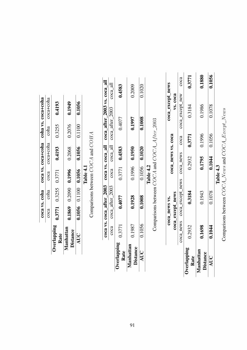
coca

vs.c

oha

coca

vs.c

oca+

coha

coha

vs.c

oca+

coha

coca

coha

coca

coca

+coh

aco

haco

ca+c

oha

Ove

rlap

ping

Rat

e0.

3771

0.32

550.

3771

0.41

930.

3255

0.41

93

Man

hatt

anD

ista

nce

0.18

690.

2090

0.19

960.

2068

0.20

760.

1949

AU

C0.

1056

0.11

000.

1056

0.10

560.

1100

0.10

56Ta

ble

4.1

Com

pari

sons

betw

eenCOCA

andCOHA

coca

vs.c

oca_

afte

r_20

03co

cavs

.coc

a_al

lco

ca_a

fter

_200

3vs

.coc

a_al

lco

caco

ca_a

fter

_200

3co

caco

ca_a

llco

ca_a

fter

_200

3co

ca_a

llO

verl

appi

ngR

ate

0.37

710.

4077

0.37

710.

4583

0.40

770.

4583

Man

hatt

anD

ista

nce

0.19

870.

1928

0.19

960.

1950

0.19

970.

2009

AU

C0.

1056

0.10

080.

1056

0.10

200.

1008

0.10

20Ta

ble

4.2

Com

pari

sons

betw

eenCOCA

andCOCA

_After_

2003

coca

_new

svs.

coca

_exc

ept_

new

sco

ca_n

ewsv

s.co

caco

ca_e

xcep

t_ne

ws

vs.c

oca

coca

_new

sco

ca_e

xcep

t_ne

ws

coca

_new

sco

caco

ca_e

xcep

t_ne

wco

caO

verl

appi

ngR

ate

0.29

320.

3184

0.29

320.

3771

0.31

840.

3771

Man

hatt

anD

ista

nce

0.16

980.

1943

0.17

950.

1996

0.19

860.

1880

AU

C0.

1044

0.10

780.

1044

0.10

560.

1078

0.10

56Ta

ble

4.3

Com

pari

sons

betw

eenCOCA

_News

andCOCA

_Except

_News

91

mon terms; and, thus we can give general guidance to the selection of

background corpus for FSD that a smaller recent domain-related corpus

will be more suitable than a very large-scale general corpus for FSD. Of

course, our research is directed only at the general situations, as the test

cases do not include extreme situations such as extremely large or small

scale of common terms. It is also worth noting that we are purposefully

focusing here on the case of a static background corpus and not on the

case of updates being made to the TF-IDF model as the FSD process

unfolds.

4.6 Summary

In this chapter, we looked into the details of the static TF-IDF mod-

els, and found two key factors relevant to terms and background cor-

pora that affect the FSD performance: the scale of common terms and

the distributional similarity between corpora. In order to evaluate these

factors, we proposed a set of metrics to quantitatively measure the scale

of common terms and the term distributional similarity of a background

corpus relative to a target corpus, and developed a pairwise comparison

scheme between two different background corpora. We also applied the

proposed metrics and comparison scheme to the comparisons between

background corpora relative to the target FSD corpus, and our results in-

dicate that term distributional similarity is more predictive of good FSD

92

performance than the scale of common terms. Finally, we answered the

research question of whether bigger or similar corpora are more useful

for FSD by showing that a smaller recent domain-related corpus will be

more suitable than a very large-scale general corpus to generate good

representations for FSD.

From the theoretical and empirical analysis in this chapter, we can

also find that terms play a very important role in the detection of a

new event, which corresponds with our findings in Chapter 3. In the

next chapter, we move on from the static TF-IDF models with the fixed

vocabulary and IDF dictionary to dynamic models, in which the vocabu-

lary and IDF dictionary are updated incrementally as the detection goes

on, and specifically investigate how the new terms in the target corpus

influence the performance of FSD.

93

Chapter 5

Dynamic Model Updates for First

Story Detection

As discussed in the last chapter, the static TF-IDF model can only take

advantage of the common terms between the background and target cor-

pus, and all the new terms from the target corpus that are unseen in the

background corpus will be ignored, which obviously causes a loss of

information.

This issue is also known as the out-of-vocabulary (OOV) problem,

which is a common problem in NLP (Manning et al., 1999), and there

are a few methods that can be used to alleviate it: 1) A simple method to

deal with it is to introduce a special token (e.g., <unk>) into the vocabu-

lary to represent all terms that are very rare in training, and then use the

special token to represent the OOV words encountered after the training

process (Jurafsky, 2000; Habash, 2008; Wołk and Marasek, 2015). 2)

Smoothing is another widely used method for handling OOV words, in

94

which the weights of OOV words are calculated based on a pre-defined

scheme (Gale and Sampson, 1995; Chen and Goodman, 1999; Valcarce

et al., 2016). For example, the add-one smoothing just assumes the oc-

currence of each OOV word to be 1 in training data (Schütze et al.,

2008). 3) Another method to mitigate the OOV problem in NLP is us-

ing subwords (e.g., character-level n-grams) to represent texts, and any

OOV word can be represented by the combination of multiple subwords

(Szoke et al., 2008; He et al., 2014; Kurniawan and Louvan, 2018).

However, specifically for the FSD task, these three methods are more

or less problematic. The method with the special token represents a

large range of terms with one single token, and thus makes it impossible

to distinguish different new terms that emerge during detection, which

is similar to a static TF-IDF model. The smoothing method normally

assumes a very low occurrence for each new term all the time, and

thus always leads to unreasonable large weights for the terms unseen in

the background corpus. Meanwhile, the subword-based models, which

hugely enlarge the vocabulary, has been shown to be neither efficient nor

effective for the FSD task (Callan et al., 1992; Allan et al., 1999). There-

fore, a dynamic TF-IDF model, in which the vocabulary and document

frequencies are incrementally updated during detection, is more suitable

for FSD and thus widely adopted (Yang et al., 1998; Brants et al., 2003;

Kannan et al., 2018a).

Very little previous research has investigated how a dynamic term

95

vector model works in practice for FSD, or has investigated how to select

hyper-parameters (such as the model update frequency) and background

corpora for such dynamic models. In this chapter, we first theoretically

analyse how a dynamic TF-IDF model works for FSD, and then em-

pirically evaluate the impact of different update frequencies and back-

ground corpora on FSD performance. Our results show that dynamic

models with high update frequencies outperform static models and dy-

namic models with low update frequencies; and, importantly, also show

that the FSD performance of dynamic models does not always increase

along with increases in the update frequency. Moreover, we demon-

strate that different background corpora have very limited influence on

the dynamic models with high update frequencies in terms of FSD per-

formance. Finally, we claim that one underlying reason that leads to all

these performances is that the new terms with large rough weights play

a more important role than the well-calculated weights and thus are a

key factor for the detection of a new event.

We organise the structure of this chapter as follow: we start from the

introduction to the dynamic TF-IDF models and how they operate for

FSD in Section 5.1. After that, we design and implement experiments to

make comparisons across different update frequencies and background

corpora in Section 5.2. Then, in Section 5.3, we analyse the reasons that

underlie the results. Finally, we draw a summary in Section 5.4.

96

5.1 Dynamic TF-IDF Models for First Story Detection

Different from the TF-IDF model in Eq. 2.6 and 2.7, for the dynamic

TF-IDF model we adjust the equations sightly. Specifically, we adopt

the following equations:

tf -idf(t, d) = tf(t, d)× idf(t)′ (5.1)

idf(t)′ = logN ′

df(t)′ (5.2)

where tf(t, d) remains the same as that in Equation 2.6, but the calcula-

tion of the IDF component idf(t)′ now makes use of an N ′ that captures

the total number of not only the documents in the background corpus

but also the stories in the target FSD corpus up to the present point, and,

similarly, df(t)′ refers to the number of documents across both the back-

ground corpus, and the portion of target corpus to the current point, that

contain the term t.

Due to the dynamic nature of this TF-IDF model, the length and fea-

ture types captured by a document vector now vary as we move through

events, and this has potential implications to the FSD process. To il-

lustrate, let us consider two documents (one being our target story and

the other some story that has already been processed by our model).

The comparison of these two documents is typically achieved with the

widely-used cosine distance in Eq. 2.8:

In order to better understand how a dynamic model performs for FSD,

97

in Table 5.1, we unfold these two document vectors to m term features

from t1 to tm, where m is the length of the current vocabulary. In a

dynamic model, the vocabulary includes both terms that were present in

the background corpus and new terms that are added during the updates

to the model. However, irrespective of whether a term is a new term or

not, the value for a term in the TF-IDF document representation is the

weight of the specific term based on the current dynamic TF-IDF model,

i.e., the vocabulary and the IDF values.

Table 5.1Two document representation vectors based on a dynamic TF-IDF model

Range A Range Bt1 ... ti ti+1 ... tm

~d v1 ... vi vi+1 ... vm

~d′ v′1 ... v′

i v′i+1 ... v′

m

In order to analyse how a TF-IDF representation treats both old and

new terms in a document representation we divide the features in our

document representation into two parts: Range A which includes terms

that have been present in the model for a substantial amount of time (be-

cause they were present in the background corpus or were added to the

model several updates previously); and Range B which includes terms

that have been added to the model recently.

In a static TF-IDF model there are only terms in Range A coming

from the background corpus, and no term in Range B since the target

corpus is not incorporated into the building of the TF-IDF model. Thus,

the performance of the TF-IDF model depends on how well the weights

98

from the background corpus represent the terms in the target corpus. As

the term weights are only calculated based on the background corpus,

the selection of the background corpus has a great impact on the static

TF-IDF model, and also influences the FSD performance just as shown

in Chapter 4. Thus, a large-scale domain-related background corpus is

normally adopted to generate realistic weights for the terms.

For a dynamic TF-IDF model, however, although it can use a large

background corpus initially, new terms that are unseen in the back-

ground corpus will emerge and be incorporated into the model as de-

tection proceeds – thus forming Range B. By definition these new terms

did not occur in the background corpus, this may be because the new

terms are genuinely rare in language, or else it may be because the se-

lected background corpus was not representative of the language in the

target data stream that the model is processing, or finally the new term

may be a true neologism in a language.

Whatever the true cause for why a particular term is a new term for a

model, the weights of these new terms may be not well calibrated with

respect to the weights for the terms in Range A. In Eq. 5.2, df(t)′ denotes

the number of documents that contain the term t not only in the already-

processed target stories, but also in the documents of the background

corpus. However, by definition new terms in Range B will not have

appeared in the background corpus and will only have appeared in the

most recent documents in the target data stream. Therefore, the value of

99

df(t)′ of a new term in Range B will be very small compared to N ′ in

Eq. 5.2, and thus the TF-IDF weights for these new terms are normally

very large, so we call these the rough weights with respect to the realistic

weights in Range A. In the calculations of cosine distance in Eq. 2.8,

more attention is focused on the features with larger values, and thus,

the terms in Range B have a bigger effect on comparison calculations

based on a dynamic TF-IDF model than they are expected to have based

on the language.1

From the analysis above, we find that a key difference between dy-

namic and static TF-IDF models, when making comparisons between

document vectors, is that dynamic models pay more attentions on the

new terms with large rough weights that emerge during detection, wher-

eas static models focus only on the existing terms whose weights are

calculated only based on the background corpus. In order to improve a

static model, or indeed the static elements of a dynamic model, we can

try to find a more suitable background corpus in order to generate real-

istic weights for the terms in the target data stream. However, for the

dynamic approach it is hard to improve performance from a theoretical

perspective due to the way in which weights are calculated for newly

encountered terms. To overcome this limitation and try to optimise the

1It is worth noting that if looking at the whole FSD process rather than the comparison between twospecific document vectors, new terms keep on being added into Range B as the updates are implemented.On the other hand, the terms already existing in Range B keep on being moved to Range A as more andmore new stories arrive and the number of stories since the term’s first appearance becomes large enoughto generate realistic weights.

100

dynamic aspects of TF-IDF modelling for FSD, in the next section we

present an experimental analysis to investigate the impact of update fre-

quency and background corpus on the model.

5.2 Experimental Design and Results

In the following, we present our experimental design and results for

evaluating the impact of the dynamic aspects of a TF-IDF model in the

context of the FSD task. We focus on the impact of different update

frequencies and the relevance of background corpora selection.

5.2.1 Experimental Design

In our experiments, we continue to use the benchmark TDT5 corpus as

target corpus for FSD detection, and COHA, COCA, COCA_News

and COCA_Except_News (introduced in Section 4.3) as the back-

ground corpora to be used as the basis of evaluation.

There is no standard update frequency for a dynamic TF-IDF model.

Typically, updates are implemented so as to be less frequent than every

100 documents (Kannan et al., 2018a), as the update process is very

expensive if the update frequency is higher than every 100 documents.

In our experiments, we evaluate a range of update frequencies - spe-

cifically, every 100, 500, 1000, 10000 and 100000 documents, and also

implement a static TF-IDF model as a baseline. The static model can be

101

interpreted as a dynamic model where updates are extremely infrequent.

For each update frequency we build TF-IDF models for all background

corpora.

Similarly to the experiments in Chapter 4, our implementation of

FSD here is also based on the nearest neighbour model with the cosine

distance adopted as the dissimilarity measure between documents. In

the pre-processing we remove stopwords and typos for all background

and target corpora, and subsequently stem all remaining terms. Align-

ing with previous research (Yang et al., 1998), comparisons are only

implemented with the time window of 2000 most recent stories for each

incoming story. The FSD results are evaluated using the AUC scores of

the DET curves as metrics for quantitative comparisons.

5.2.2 Comparisons across Different Update Frequencies

We begin by examining the FSD performance results as influenced by

update frequency. From the results shown in Figure 5.1, we firstly see a

trend that for each background corpus, the dynamic TF-IDF models with

very high update frequencies, i.e., every 100, 500 and 1000 documents,

generally outperform dynamic models with very low update frequencies,

i.e., every 100000 documents, and the static model, which can also be

considered as a dynamic model with a very high update frequency2.

2The results for the dynamic model with a medium update frequency, i.e., every 10,000 documents,show no clear trend, but the trend is very clear in the comparison between the dynamic models with veryhigh and very low update frequencies

102

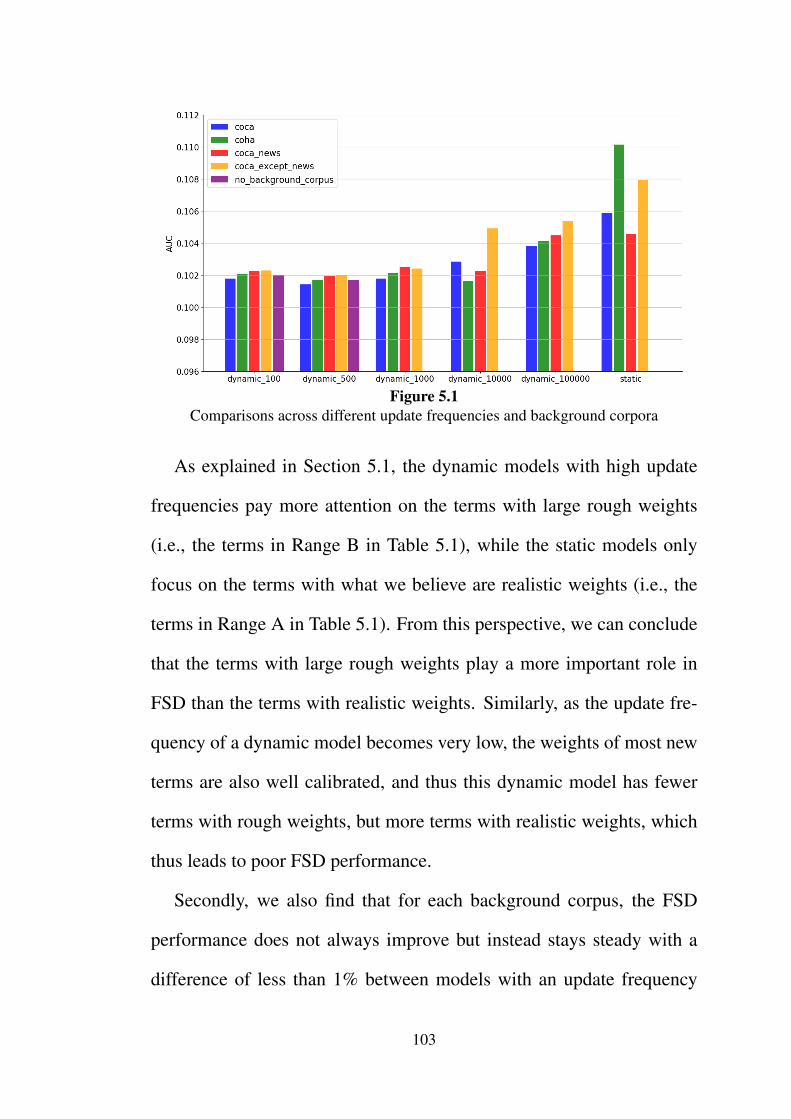
Figure 5.1Comparisons across different update frequencies and background corpora

As explained in Section 5.1, the dynamic models with high update

frequencies pay more attention on the terms with large rough weights

(i.e., the terms in Range B in Table 5.1), while the static models only

focus on the terms with what we believe are realistic weights (i.e., the

terms in Range A in Table 5.1). From this perspective, we can conclude

that the terms with large rough weights play a more important role in

FSD than the terms with realistic weights. Similarly, as the update fre-

quency of a dynamic model becomes very low, the weights of most new

terms are also well calibrated, and thus this dynamic model has fewer

terms with rough weights, but more terms with realistic weights, which

thus leads to poor FSD performance.

Secondly, we also find that for each background corpus, the FSD

performance does not always improve but instead stays steady with a

difference of less than 1% between models with an update frequency

103

higher than every 1000 documents. One potential reason for this may

be that as we increase the update frequency there are two counteracting

processes with respect to rough weights: (a) a high update frequency

means that new terms with rough weights are introduced into the model

frequently, but (b) a high update frequency also means that the already-

existing rough weights will themselves be updated incrementally and so

may be smoothed frequently, and, thus they do not stay rough for long.

5.2.3 Comparisons across Different Background Corpora

In order to facilitate the selection of background corpora for dynamic

TF-IDF models, we also analyse the results from a different perspective

by making comparisons across different background corpora. From Fig-

ure 5.1, it can also be seen that the differences caused by different back-

ground corpora are only noteworthy in the static model and dynamic

models with low update frequencies. In the dynamic models with high

update frequencies such as every 100, 500, 1000 stories, the influences

are minor (less than 1%). This raises the possibility that models with

high update frequencies are not affected by the choice of background

corpus, in which case it may be possible to achieve good performance

with a relatively small background corpus.

104

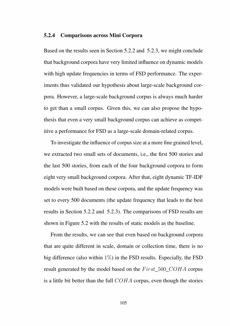
5.2.4 Comparisons across Mini Corpora

Based on the results seen in Section 5.2.2 and 5.2.3, we might conclude

that background corpora have very limited influence on dynamic models

with high update frequencies in terms of FSD performance. The exper-

iments thus validated our hypothesis about large-scale background cor-

pora. However, a large-scale background corpus is always much harder

to get than a small corpus. Given this, we can also propose the hypo-

thesis that even a very small background corpus can achieve as compet-

itive a performance for FSD as a large-scale domain-related corpus.

To investigate the influence of corpus size at a more fine grained level,

we extracted two small sets of documents, i.e., the first 500 stories and

the last 500 stories, from each of the four background corpora to form

eight very small background corpora. After that, eight dynamic TF-IDF

models were built based on these corpora, and the update frequency was

set to every 500 documents (the update frequency that leads to the best

results in Section 5.2.2 and 5.2.3). The comparisons of FSD results are

shown in Figure 5.2 with the results of static models as the baseline.

From the results, we can see that even based on background corpora

that are quite different in scale, domain or collection time, there is no

big difference (also within 1%) in the FSD results. Especially, the FSD

result generated by the model based on the First_500_COHA corpus

is a little bit better than the full COHA corpus, even though the stories

105

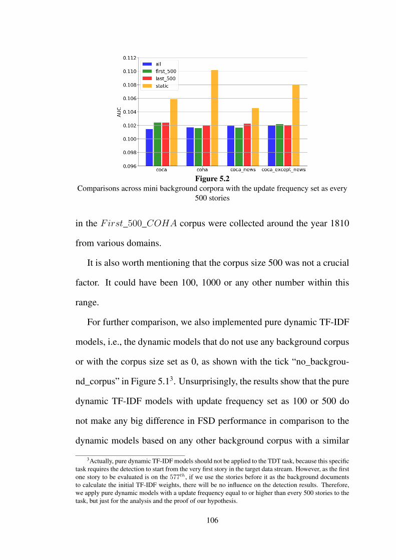
Figure 5.2Comparisons across mini background corpora with the update frequency set as every

500 stories

in the First_500_COHA corpus were collected around the year 1810

from various domains.

It is also worth mentioning that the corpus size 500 was not a crucial

factor. It could have been 100, 1000 or any other number within this

range.

For further comparison, we also implemented pure dynamic TF-IDF

models, i.e., the dynamic models that do not use any background corpus

or with the corpus size set as 0, as shown with the tick “no_backgrou-

nd_corpus” in Figure 5.13. Unsurprisingly, the results show that the pure

dynamic TF-IDF models with update frequency set as 100 or 500 do

not make any big difference in FSD performance in comparison to the

dynamic models based on any other background corpus with a similar

3Actually, pure dynamic TF-IDF models should not be applied to the TDT task, because this specifictask requires the detection to start from the very first story in the target data stream. However, as the firstone story to be evaluated is on the 577th, if we use the stories before it as the background documentsto calculate the initial TF-IDF weights, there will be no influence on the detection results. Therefore,we apply pure dynamic models with a update frequency equal to or higher than every 500 stories to thetask, but just for the analysis and the proof of our hypothesis.

106

update frequency, and this finding supports our conclusion that back-

ground corpora have very limited influence on dynamic models with

high update frequencies in terms of FSD performance.

5.3 Discussion

In order to explain the experimental results in the last section, we need

a deeper understanding of how the dynamic model works for FSD in the

nearest neighbour algorithm. Specifically, we need a deeper understand-

ing of the influence of the terms with large rough weights in Range B

from Table 5.1 in different situations of comparison between an incom-

ing story and an existing story. Furthermore, we need to explore how

we can better take advantage of the findings of this analysis. To simplify

the interpretation, we use "rough terms" in this section to refer to "terms

with large rough weights in Range B from Table 5.1"

5.3.1 Effect of Rough Terms in the Calculations

First of all, there are two main situations where an incoming story is

compared with an existing story: (1) the incoming story does NOT con-

tain any rough term that exists only in the incoming story but not in

any existing story; and (2) the incoming story DOES contain the kind

of terms in (1) (e.g., the brand new terms that emerge for this first time

in the incoming story). For each situation, there are four sub-situations

107

depending on whether the incoming story and the existing story being

compared contain any common rough term, and whether the existing

story contains rough terms that do not exist in the incoming story. We

summarise all these situations as follows:

1. The incoming story does not contain any rough term that only ex-

ists in the incoming story but not in any previous existing story.

Under this main situation, there are four sub-situations in the com-

parison between an incoming story and a existing story:

1.1. Nether the incoming story nor the existing story contains any

rough term. In this case, the cosine distance is calculated only

based on terms with reasonable weights (in Range A);

1.2. The existing story contains only common rough terms with the

incoming story, but does not contain any rough term that do not

exist in the incoming story. In this case, as the weights of rough

terms are relatively higher than the reasonably-calculated we-

ights, the calculation of the cosine distance mainly depends

on these common rough terms between the existing story and

the incoming story. However, because the rough weights are

calculated only based on a small number of documents, this

situation is difficult to investigate further;

1.3. The existing story does not contain any common rough term

with the incoming story, but contains rough terms that do not

108

exist in the incoming story. In this case, as the rough terms

only exist in the existing story, the weights of the rough terms

are large positive numbers for the existing story, but 0 for the

incoming story. Form the calculation of cosine distance, we

can see that this kind of term features does not affect the dot

product on the numerator at all, but results in a bigger denom-

inator. Therefore, the cosine distance from the existing story to

the incoming story will be relatively large. As we are looking

for the nearest neighbour, i.e., the existing story with the smal-

lest cosine distance to the incoming story, the existing story in

this situation will probably be less likely to be selected as the

nearest neighbour than the existing stories in situation 1.1 and

1.2;

1.4. The existing story contains not only common rough terms with

the incoming story, but also the rough terms that do not exists

in the incoming story. This situation is similar to situation 1.3,

and also results in a large cosine distance and thus reduces the

likelihood that the existing story will be selected as the nearest

neighbor.

2. The incoming story contains rough terms that only exist in the in-

coming story but not in any previous existing story. There are also

four similar sub-situations for this main situation just as from 1.1 to

109

1.4. However, because of the rough terms that only exist in the in-

coming story, all these four sub-situations results in a large cosine

distance just as the situations 1.3 and 1.4, and we just take them

together to be situation 2.

These situations are also summarised in Table 5.2.

If we assume that new terms are an important indicator of new events,

i.e., different events are associated with different terms and new terms

emerge in new events, it can be found that the dynamic models can help

FSD detection in (a) building more accurate TF-IDF weights by updat-

ing weights in Range A, so as to improve the general performance in

the situation 1.1; (b) distinguishing stories about different events in situ-

ation 1.3 and 1.4, so as to reduce the False Alarm rate; (c) indicating an

incoming story that discusses a new event in situation 2, so as to reduce

the Miss rate. Only in the situation 1.2, it is hard to say how the dynam-

ics works because the comparison depends on the roughly calculated

weights.

In terms of the selection of update frequency, when the update fre-

quency gets higher, we find: (a) the model updates the TF-IDF weights

in time, and thus improve the situation 1.1; (b) there are more rough

terms in the dynamic model with high frequency like f=100, than the

model with low frequency like f=100000, because when the model up-

dates infrequently, only the last small part of stories can cause roughly-

calculated weights, e.g., the last 100 stories in the dynamic model with

110

Tabl

e5.

2D

iffer

ents

ituat

ions

whe

nco

mpa

ring

anin

com

ing

stor

yw

ithan

exis

ting

stor

y

Situ

atio

nsW

heth

erth

ein

com

ing

stor

yco

ntai

nsro

ugh

term

sth

aton

lyex

isti

nth

ein

com

ing

stor

ybu

tnot

inan

ypr

evio

usex

istin

gst

ory

Whe

ther

the

inco

min

gst

ory

and

the

exis

ting

stor

ybe

ing

com

pare

dco

ntai

nan

yco

mm

onro

ugh

term

Whe

ther

the

exis

ting

stor

yco

ntai

nsro

ugh

term

sth

atdo

note

xist

inth

ein

com

ing

stor

y1.

1N

oN

oN

o1.

2N

oY

esN

o1.

3N

oN

oY

es1.

4N

oY

esY

es

2

Yes

No

No

Yes

Yes

No

Yes

No

Yes

Yes

Yes

Yes

111

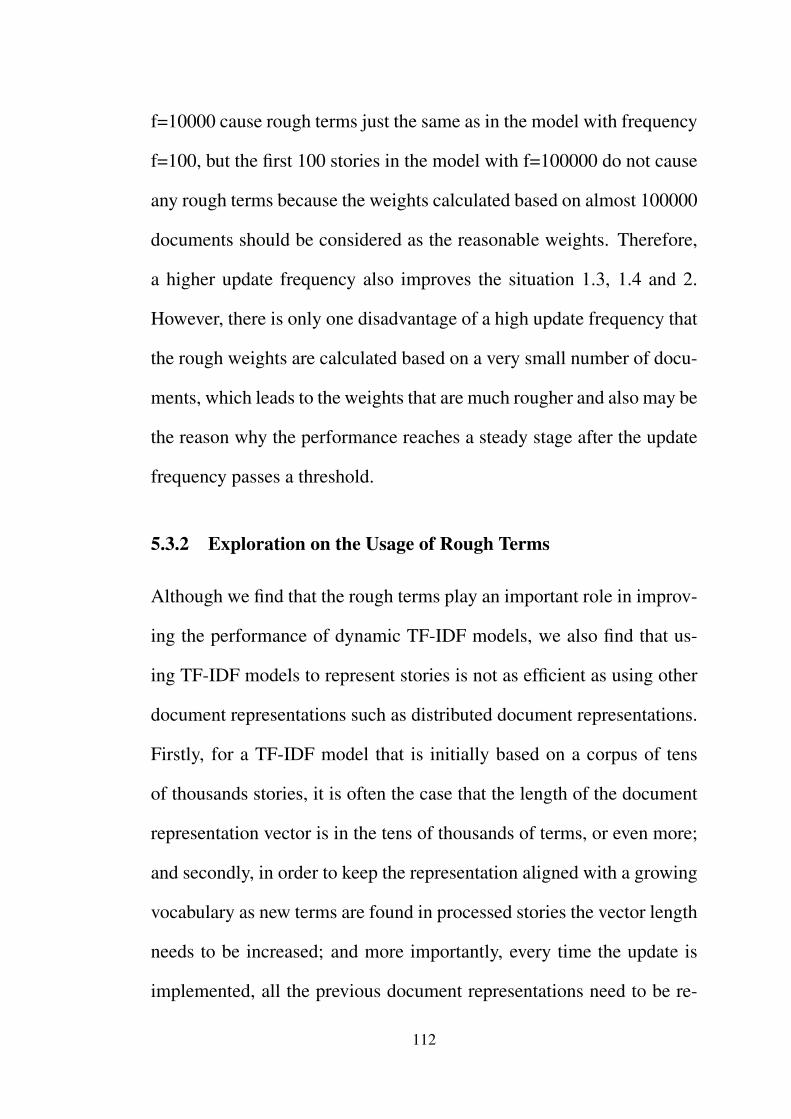
f=10000 cause rough terms just the same as in the model with frequency

f=100, but the first 100 stories in the model with f=100000 do not cause

any rough terms because the weights calculated based on almost 100000

documents should be considered as the reasonable weights. Therefore,

a higher update frequency also improves the situation 1.3, 1.4 and 2.

However, there is only one disadvantage of a high update frequency that

the rough weights are calculated based on a very small number of docu-

ments, which leads to the weights that are much rougher and also may be

the reason why the performance reaches a steady stage after the update

frequency passes a threshold.

5.3.2 Exploration on the Usage of Rough Terms

Although we find that the rough terms play an important role in improv-

ing the performance of dynamic TF-IDF models, we also find that us-

ing TF-IDF models to represent stories is not as efficient as using other

document representations such as distributed document representations.

Firstly, for a TF-IDF model that is initially based on a corpus of tens

of thousands stories, it is often the case that the length of the document

representation vector is in the tens of thousands of terms, or even more;

and secondly, in order to keep the representation aligned with a growing

vocabulary as new terms are found in processed stories the vector length

needs to be increased; and more importantly, every time the update is

implemented, all the previous document representations need to be re-

112

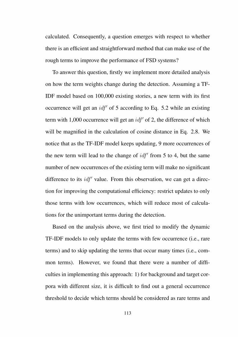
calculated. Consequently, a question emerges with respect to whether

there is an efficient and straightforward method that can make use of the

rough terms to improve the performance of FSD systems?

To answer this question, firstly we implement more detailed analysis

on how the term weights change during the detection. Assuming a TF-

IDF model based on 100,000 existing stories, a new term with its first

occurrence will get an idf ′ of 5 according to Eq. 5.2 while an existing

term with 1,000 occurrence will get an idf ′ of 2, the difference of which

will be magnified in the calculation of cosine distance in Eq. 2.8. We

notice that as the TF-IDF model keeps updating, 9 more occurrences of

the new term will lead to the change of idf ′ from 5 to 4, but the same

number of new occurrences of the existing term will make no significant

difference to its idf ′ value. From this observation, we can get a direc-

tion for improving the computational efficiency: restrict updates to only

those terms with low occurrences, which will reduce most of calcula-

tions for the unimportant terms during the detection.

Based on the analysis above, we first tried to modify the dynamic

TF-IDF models to only update the terms with few occurrence (i.e., rare

terms) and to skip updating the terms that occur many times (i.e., com-

mon terms). However, we found that there were a number of diffi-

culties in implementing this approach: 1) for background and target cor-

pora with different size, it is difficult to find out a general occurrence

threshold to decide which terms should be considered as rare terms and

113

need to be updated; 2) as the detection goes on for a long time, the

amount of stories that arrived during the detection becomes compar-

able with or even larger than the amount of stories used initially for the

weight calculation, and in this situation, the weight updates on the com-

mon terms also cannot be neglected; 3) even we can find a reasonable

way to update only the rare terms, all the previous document representa-

tions still need to be re-calculated every time the update is implemented,

and thus the detection process is still computational expensive. There-

fore, we need to look at this problem from a different perspective, and

try to find out an efficient way to take advantage of our findings relat-

ing to TF-IDF models. We will introduce our proposed New Term Rate

(NTR) method in the next chapter.

5.4 Summary

In this chapter we empirically validated that the dynamic TF-IDF mod-

els with high update frequencies outperform the static model and the dy-

namic models with low update frequencies, and found that the FSD per-

formance of dynamic models does not always improve but stays steady

as the update frequency goes beyond some threshold, and that the back-

ground corpora have very limited influence on the dynamic models with

high update frequencies in terms of FSD performance. Consequently,

we claim that the best TF-IDF model for FSD should be a dynamic

114

model whose weights are initially calculated based on any small-size

corpus but updated with a reasonable high frequency, e.g., for our scen-

ario we found an update frequency of every 500 stories results in good

performance. Based on this, we set out some factors that may explain

these findings. However, a key element of these explanations is the ob-

servation that a high update frequency can result in new terms with large

rough weights being introduced into the TF-IDF representations. In the

next chapter, we will explore an efficient and straightforward way to

exploit the new terms to improve the FSD performance.

115

Chapter 6

The New Term Rate Method

As discussed in last chapter, the nearest neighbour model with the dy-

namic TF-IDF representations outperforms other FSD systems poten-

tially because the new terms with roughly-calculated large weights play

an important role. However, we also notice that the cost of taking ad-

vantage of the new terms is very high using the dynamic TF-IDF doc-

ument representations: as the detection proceeds, more and more new

terms are taken into account, which ultimately results in a very large

vocabulary. This is also why most previous research has adopted a fixed

vocabulary. We thus tried to find some way to implement the updat-

ing efficiently, e.g., only update the rare terms rather than all the terms.

However, even if we could overcome the difficulties highlighted in the

previous chapter and realise this idea, the method would still be com-

putational expensive because all the previous representations need to

be re-calculated as long as the update is implemented. Consequently,

we need to find an efficient and straightforward method that can make

116

use of the rough terms to improve the performance of FSD systems. In

this chapter, we propose the New Term Rate (NTR) method that can

be implemented efficiently but makes significant improvement on the

performance of most FSD systems with different detection models and

document representations for different types of target corpora.

We organise the structure of this chapter as follow: we first introduce

the motivation of the idea before proposing the new term rate metric

and the NTR method in Section 6.2, and then present the verification of

the effectiveness of the NTR method in Section 6.3. In Section 6.4, we

discuss the selection of the parameters in the method, followed by the

summary in Section 6.5.

6.1 Motivation

As discuss in Section 5.3, although we have identified the importance

of rough terms in the dynamic TF-IDF models, we believe that in order

to keep our models efficient during updates we shoudl keep the TF-IDF

model stable, and explore a new ways to extend the TF-IDF model that

enables the model to make the best use of the rough terms. Specifically,

we make exploration from two perspectives:

- Focusing on only the new terms: since it is difficult to find out

a threshold to distinguish rare terms from common terms and un-

reasonable to always keep the weights of common terms fixed, we

117

simplify this problem by only focusing on the new terms that have

never occured before or at least did not occur within a history of k

stories. In this way, we do not need an occurrence threshold, and

instead make the decision of whether to update a terms based on

whether it has been seen recently;

- Using an independent factor: we know it is computational ex-

pensive to use TF-IDF models because they can only represent

a term with a single feature/dimension. We explore the efficient

exploitation of new terms by designing an independent factor to

represent this information and merging it with the novelty scores

generated by normal FSD models.

In the following sections, we will present how our proposed method

works and verify its effectiveness in a variety of situations.

6.2 The New Term Rate Method

Based on our analysis in Sections 5.3 and 6.1, we aim to design a factor

to evaluate the scale of the new terms in a candidate story. With this

factor integrated into the novelty scores generated by normal FSD mod-

els, new novelty scores can be generated that include the information of

the new terms but still retain the original information of previous FSD

systems.

118

6.2.1 Newe Term Rate

Intuitively, we define a new metric, the new term rate, to represent the

proportion of new terms in a story d given a history of k stories. This is

expressed as follows:

new_term_rate(d, k) = nnew(d, k)N(d) (6.1)

where d denotes the candidate story and k refers to the number of most

recent stories for which the new terms are defined, i.e., if a term does not

occur in the most recent k stories, we say this term is a new term, and

nnew(d, k) and N(d) are respectively the number of new terms given a

history of k stories and the number of all the terms of the story d. The

new term has a range of [0,1].

Our assumption is that a large new term rate can help indicate a first

story. However, the new term rate itself is too simple to be used as the

novelty score for the FSD detection, which will be shown in Section

6.3.2; on the other hand, if applied with other FSD systems, the new

term rate can be used to weight the novelty scores normally generated

by other FSD models.

6.2.2 The New Term Rate Method

Based on the new term rate, we further propose the New Term Rate

(NTR) method for FSD. After a baseline FSD system has generated a

119

novelty score for the candidate story, we weight the original novelty

score by multiplying by a factor formed by the new term rate, and gen-

erate a new novelty score for each candidate story as follows:

new_novelty_score(d) = original_novelty_score(d)

∗ (1 + α ∗ new_term_rate(d, k))(6.2)

where original_novelty_score(d) and new_novelty_score(d) are the

novelty score of the candidate story d before and after applying the NTR

method, and new_term_rate(d, k) is the new term rate we just defined

in Eq. 6.1, and α is a positive parameter to adjust the weight of the

application of new_term_rate(d, k). We give names to the two para-

meters of the NTR method, k and α, as the “history” and “NTR weight”

respectively, and will discuss the selection of them in Section 6.4.

With this method, we expect a large new term rate can magnify the

original novelty score so as to make the candidate story more compel-

ling to be detected as a first story, and a small new term rate, by contrast,

will make the candidate story unobtrusive during the detection. Con-

sequently, there is one limitation in the application of the NTR method -

the original novelty scores that the FSD systems generate must be non-

negative or can be converted into non-negative, and otherwise, the effect

of the new term rate will be opposite to expected for the negative values.

We take a simple case for example to explain this limitation. Given

120

two stories, the original novelty scores of which are −0.3 and −0.4 re-

spectively based on some specific FSD system and the corresponding

new term rates of which are 0.5 and 0.1 respectively, as it has a big-

ger original novelty score as well as a bigger new term rate, the former

story is more probably a first story than the latter one. However, be-

cause the original novelty scores are negative, the new novelty score of

the former story after applying the NTR method (e.g., α = 1) becomes

−0.3 ∗ (1 + 1 ∗ 0.5) = −0.45, which is even smaller than that of the

latter story, −0.4 ∗ (1 + 1 ∗ 0.1) = −0.44. This is obviously not what

we expect. Fortunately, in most FSD systems, the novelty scores are

calculated using measures whose results are always positive (e.g., the

Euclidean distance) or have definite scope (e.g., the cosine distance), so

this limitation rarely restricts the application of the NTR method, ex-

cept in some special cases like the one class SVM detection model we

discussed in Chapter 3.

6.2.3 Method Properties

Based on Eq. 6.1 and Eq. 6.2, we can also find some explicit properties

of the NTR method as follows:

1. Non-invasive. As it multiplies the factor to the novelty scores that

are already generated by the FSD systems, the NTR method does

nothing with the original systems, and thus the original systems can

generate novelty scores just as they used to do. Therefore, we say

121

the NTR method is non-invasive to the original FSD systems.

2. Generalisable. As discussed in Chapter 2, in both previous re-

search and practical use, FSD systems are required to generate a

novelty score for each story in the stream rather than to only label

each story as novel or old. Therefore, we can just multiply the ori-

ginal novelty score with a factor (1 + α ∗ new_term_rate(d, k))

and take their product as the new novelty score, no matter how the

novelty score is calculated for a candidate story in the original FSD

system. Therefore, the NTR method is a generalisable method that

can be applied to a large variety of FSD systems.

3. Efficient and Straightforward. It is also easily found from the Eq.

6.1 that the time complexity of the calculation of the new term rate

is estimated as O(N(d)), where N(d) is the number of all terms of

a candidate story d as mentioned above, so the NTR method only

brings in lightweight extra computation and thus is computation-

ally cheap. Additionally, from Eq. 6.2 we can also find that given

the original novelty score and the new term rate the implementa-

tion of the NTR method is very simple to make only three times of

basic addition or multiplication operations. Therefore, we say the

NTR method is both efficient and straightforward.

In spite of these good properties, there is one point that are note-

worthy in the implementation of the NTR method: although the NTR

122

method is non-invasive with respect to the original FSD systems, the

value of a proper threshold probably differs from that of the original

FSD model after the NTR method is applied, because the selection of

the proper threshold is made after the generation of the final novelty

score and thus the range of the final novelty scores changes after the

multiplication of the factor (1 + α ∗ new_term_rate(d, k)).

6.2.4 The Distinct New Term Rate Method

As shown above, we design the new term rate and the NTR method

based on the number of new terms and all the terms in a candidate doc-

ument. However, during the research process, we also tried a different

approach in which the new term rate and the method are calculated based

on the number of distinct new terms and all the distinct terms in the can-

didate document. In this way, we focus only on the occurrence of terms

but ignore the frequency of the occurrence. Specifically, the new term

rate metric in Eq. 6.1 is modified to:

distinct_new_term_rate(d, k) = distinct_nnew(d, k)distinct_N(d) (6.3)

where the distinct_nnew(d, k) and distinct_N(d) are respectively the

number of distinct new terms given a history of k stories and the number

of all the distinct terms of the story d, and the NTR method in Eq. 6.2 is

123

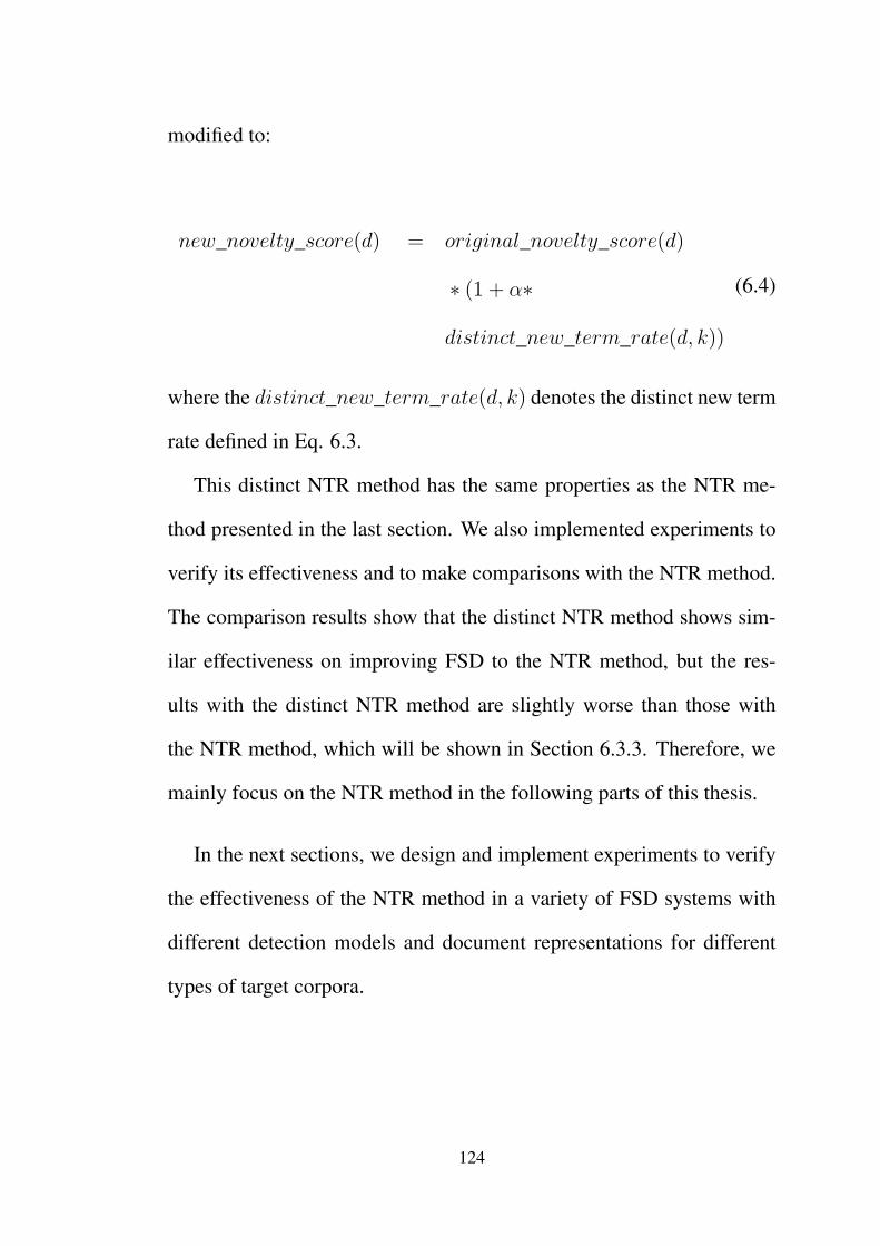
modified to:

new_novelty_score(d) = original_novelty_score(d)

∗ (1 + α∗

distinct_new_term_rate(d, k))

(6.4)

where the distinct_new_term_rate(d, k) denotes the distinct new term

rate defined in Eq. 6.3.

This distinct NTR method has the same properties as the NTR me-

thod presented in the last section. We also implemented experiments to

verify its effectiveness and to make comparisons with the NTR method.

The comparison results show that the distinct NTR method shows sim-

ilar effectiveness on improving FSD to the NTR method, but the res-

ults with the distinct NTR method are slightly worse than those with

the NTR method, which will be shown in Section 6.3.3. Therefore, we

mainly focus on the NTR method in the following parts of this thesis.

In the next sections, we design and implement experiments to verify

the effectiveness of the NTR method in a variety of FSD systems with

different detection models and document representations for different

types of target corpora.

124

6.3 Experimental Verification

In this section, we design and implement experiments to verify our pro-

posed NTR method.

6.3.1 Experimental Design

In total we implement four sets of experiments for the verification of

the application of the NTR method to different FSD systems and target

corpora as follows:

- Exp. 1: verification in different background corpora for TF-IDF

document representations;

- Exp. 2: verification in different types of document representations;

- Exp. 3: verification in different types of FSD models;

- Exp. 4: verification in a different type of target corpora.

The main target corpora used in these experiments is the standard

benchmark target corpus - the TDT5 corpus. However, in the case of

Exp. 4 we also make use of the Twitter target corpus. Before detection,

all data, in both the background and target corpora, is pre-processed

just as in previous chapters to reduce the influence of some unnecessary

factors like stopwords and typos.

For parameter selection, we investigate a range of values for each

of the two parameters of the NTR method - the history k and the NTR

125

weight α, and select the set of parameters that leads to the best result

for a detection system and a target corpus. The details of the parameter

selection will be discussed in Section 6.4.

The evaluation of FSD results is a bit different from that in previous

chapters, i.e., we not only use the DET curves and the AUC scores to

make comparisons between the performance of FSD systems with and

without the NTR method, but also use the Cmin metric in Eq. 2.5 to

compare our results against the current state-of-the-art results for differ-

ent target corpora.

6.3.2 Results for Reference

Although our results with the NTR method that will be shown in this

section are competitive or better than the state-of-the-art FSD system for

different target corpora, the main aim of our experiments is not to claim

the new state of the art, but to verify the effectiveness of our proposed

NTR method, in terms of improving a range of systems. Therefore, the

results of the FSD system without the NTR method are naturally taken

as the baselines, and the results with the NTR method are compared with

the corresponding baseline to find out the improvement between them as

the effect of the NTR method.

However, for general reference, we still present the state-of-the-art

FSD result for the two different types of target corpus in Table 6.1. Both

state-of-the-art results are achieved by the nearest neighbour-based LSH

126

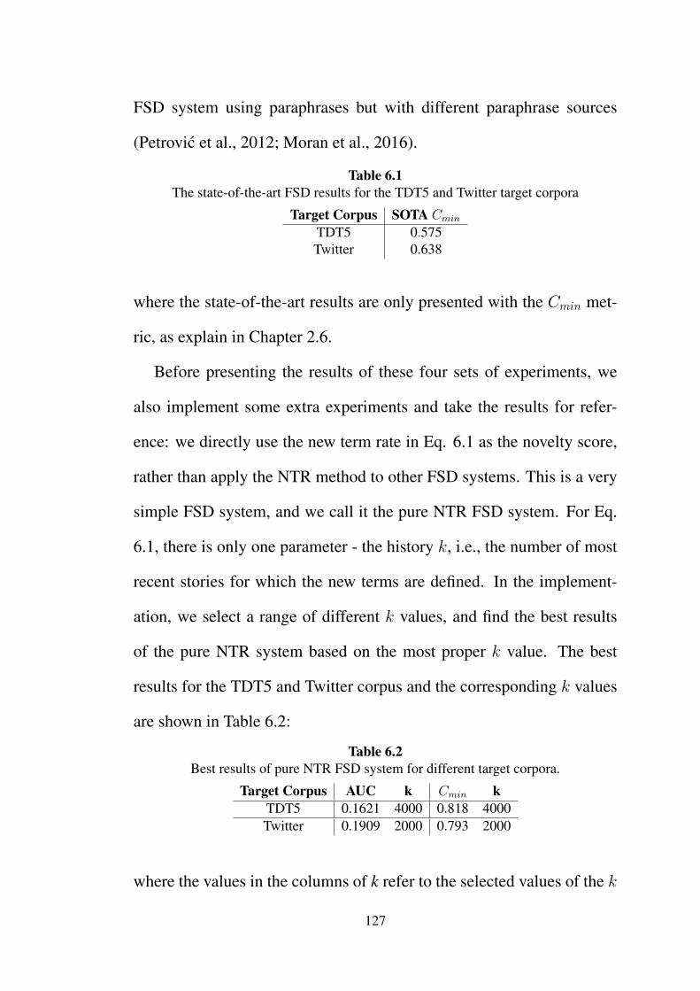
FSD system using paraphrases but with different paraphrase sources

(Petrovic et al., 2012; Moran et al., 2016).

Table 6.1The state-of-the-art FSD results for the TDT5 and Twitter target corpora

Target Corpus SOTA Cmin

TDT5 0.575Twitter 0.638

where the state-of-the-art results are only presented with the Cmin met-

ric, as explain in Chapter 2.6.

Before presenting the results of these four sets of experiments, we

also implement some extra experiments and take the results for refer-

ence: we directly use the new term rate in Eq. 6.1 as the novelty score,

rather than apply the NTR method to other FSD systems. This is a very

simple FSD system, and we call it the pure NTR FSD system. For Eq.

6.1, there is only one parameter - the history k, i.e., the number of most

recent stories for which the new terms are defined. In the implement-

ation, we select a range of different k values, and find the best results

of the pure NTR system based on the most proper k value. The best

results for the TDT5 and Twitter corpus and the corresponding k values

are shown in Table 6.2:

Table 6.2Best results of pure NTR FSD system for different target corpora.

Target Corpus AUC k Cmin kTDT5 0.1621 4000 0.818 4000Twitter 0.1909 2000 0.793 2000

where the values in the columns of k refer to the selected values of the k

127

parameter in the pure NTR FSD system that result in the best results in

the cells on their left. For example, the k value of 4,000 corresponding

to the AUC score 0.1621 for the TDT5 target corpus means that the best

performance of the pure NTR FSD system - 0.1621 in terms of the AUC

score, was achieved when the value of the history parameter k was set

as 4,000, i.e., the new terms were defined with the most recent 4,000

stories. It is clear that the performance of the pure NTR FSD system is

much worse than the state of the art shown in Table 6.1, which indicates

that the new term rate is not suitable to be applied on its own.

We can also find that for each target corpus the best AUC and Cmin

are achieved by the same parameter setting, i.e., k = 4000 for the TDT5

target corpus and k = 2000 for the Twitter target corpus. It is a usual

situation that both the best AUC and Cmin are achieved by the same FSD

system and parameter setting, but it is not always the case, because the

Cmin metric evaluates only one specific point on the DET curve, and thus

cannot guarantee exactly the same trend as the AUC score that evaluates

the whole DET curve.

6.3.3 Verification in Different Background Corpora

As the nearest neighbour-based model with the TF-IDF document rep-

resentation outperforms other FSD systems, we first implement the veri-

fication of the effectiveness of the NTR method in different background

corpora for TF-IDF document representations for the TDT5 target cor-

128

pus.

Specifically, we evaluate the results of the nearest neighbour model

with both static and dynamic TF-IDF representations based on different

basic background corpora: COCA, COHA, COCA_News,

COCA_Except_News, and their subsets. All these systems are imple-

mented with and without the NTR method with the goal to investigate

the effect of the NTR method.

In the implementation, there is no length limit for the TF-IDF repres-

entations, and the update frequencies for the dynamic TF-IDF models

are all set as every 500 stories, which is shown in Chapter 5 as a good

setting. The detection with the nearest neighbour model still uses the

time window method and only make comparisons with the most recent

2000 stories, which is the same as in previous chapters.

The results are shown in Table 6.3, in which each line shows the

comparison between results of one FSD system with and without the

NTR method.

The first four lines of results are generated by the static TF-IDF doc-

ument representations while the next four lines by the dynamic repres-

entations. The first column describes the FSD systems, specifically the

TF-IDF representations, with the background corpus denoted inside the

brackets. The next five columns present the results based on the AUC

scores, while the last five columns show the results based on the Cmin

metric. The columns with the names "without NTR" and "with NTR"

129

Tabl

e6.

3T

heef

fect

iven

ess

ofth

eN

TR

met

hod

inth

ene

ares

tnei

ghbo

urm

odel

with

the

TF-

IDF

docu

men

trep

rese

ntat

ions

fort

heT

DT

5ta

rget

corp

us

AU

CC

min

(SO

TA:0

.575

)w

ithou

tN

TR

with

NT

RIm

prov

.(%

)k

αw

ithou

tN

TR

with

NT

RIm

prov

.(%

)k

α

Stat

ic(C

OC

A)

0.10

590.

1001

5.48

%27

8108

70.

635

0.60

44.

97%

2781

0811

Stat

ic(C

OH

A)

0.11

020.

1034

6.14

%40

007

0.62

20.

606

2.66

%40

005.

2St

atic

(CO

CA

New

s)0.

1046

0.09

816.

17%

2781

087

0.63

60.

600

5.69

%27

8108

7.1

Stat

ic(C

OC

Aex

cept

New

s)0.

1079

0.10

185.

66%

2781

086

0.63

40.

605

4.50

%40

003

Dyn

amic

(CO

CA

)0.

1014

0.09

605.

37%

2781

084

0.64

10.

601

6.21

%27

8108

3D

ynam

ic(C

OH

A)

0.10

170.

0961

5.50

%27

8108

50.

654

0.59

88.

60%

2781

0812

Dyn

amic

(CO

CA

New

s)0.

1019

0.09

635.

47%

2781

084

0.62

80.

598

4.80

%27

8108

11D

ynam

ic(C

OC

Aex

cept

New

s)0.

1020

0.09

605.

91%

2781

084

0.62

80.

599

4.66

%27

8108

1

Dyn

amic

(CO

CA

New

sFi

rst5

00)

0.10

170.

0954

6.14

%27

8108

3.8

0.63

80.

584

8.43

%27

8108

4D

ynam

ic(C

OH

AFi

rst5

00)

0.10

160.

0957

5.82

%27

8108

40.

629

0.57

48.

75%

2781

082.

6

130

show the quantitative metric values of the FSD results without and with

the NTR method respectively based on the corresponding evaluation

metric. The columns with the name "Improv. (%)" shows the differ-

ence between the system with and without NTR, i.e., the improvement

by the NTR method, which is presented in percentage. The columns of k

and α indicate the corresponding parameter setting for the NTR method

that leads to the specific largest improvement in the columns on their

left.

From these results, we can firstly find that all the results with NTR are

better than those without NTR, so the improvement by the NTR method

is statistically significant. Secondly, all the improvement is noteworthy,

i.e., above 5.37% and 4.50% based on AUC and Cmin respectively, ex-

cept the only case - the improvement of 2.66% for Static (COHA) based

on Cmin.

As we discussed in Chapter 5, for the dynamic TF-IDF model with

a high update frequency, the background corpus has very little effect on

FSD results, which can also be seen from the results. However, in or-

der to set baselines for future work and make general comparisons with

other systems, we implement extra experiments for dynamic TF-IDF

models based on some very small corpora, i.e., corpora formed by the

first or the last 500 stories of the corpus COCA or COHA as in Chapter

5. The last two lines of Table 6.3 show the best results from all the sys-

tems with NTR based on AUC and Cmin respectively: the system with

131

the dynamic TF-IDF document representation based on the very small

corpus formed by the first 500 stories of COCA_News achieves the

best result based on the AUC - 0.0954; and the system with the dynamic

TF-IDF document representation based on the very small corpus formed

by the first 500 stories of COHA achieves the best result based on Cmin

- 0.574, which is competitive to and a little bit better than the current

state-of-the-art result based on Cmin - 0.575, by the LSH FSD system

using paraphrases (Petrovic et al., 2012).

The best results for the systems with and without NTR based on

either AUC or Cmin are all denoted in bold. The best results without

and with NTR based on AUC are 0.1014 and 0.0954 respectively, and

the best results based on Cmin are 0.622 and 0.574 respectively. The

improvement is 5.92% and 7.72%, which can be considered as the gen-

eral improvement by the NTR method on the systems with the nearest

neighbour model and the TF-IDF document presentation.

As mentioned in Section 6.2.4, we also implemented experiments for

the distinct NTR method and made comparisons between the effective-

ness of these two types of NTR methods. The comparison results for

TF-IDF models with different background corpora are shown in Table

6.4, and the results in bold are the better ones in comparison. From the

results, we can see that in most cases the NTR method outperforms the

distinct NTR method, including the best results for both AUC (0.0954

132

vs. 0.0959) and Cmin (0.0574 vs. 0.0579). Therefore, in the following

sections of the thesis we only focus on the NTR method and do not show

the results with the distinct NTR method.

Table 6.4The comparison between the effectiveness of the NTR method and the distinct NTR

method

AUC Cmin

d-NTR NTR d-NTR NTRStatic (COCA) 0.0999 0.1001 0.619 0.604Static (COHA) 0.1040 0.1034 0.614 0.606

Static (COCA News) 0.0984 0.0981 0.605 0.600Static (COCA except News) 0.1021 0.1018 0.615 0.605

Dynamic (COCA) 0.0963 0.0960 0.608 0.601Dynamic (COHA) 0.0965 0.0961 0.610 0.598

Dynamic (COCA News) 0.0968 0.0963 0.596 0.598Dynamic (COCA except News) 0.0964 0.0960 0.606 0.599

Dynamic (COCA News First 500) 0.0959 0.0954 0.579 0.584Dynamic (COHA First 500) 0.0962 0.0957 0.594 0.574

6.3.4 Verification in Different Types of Document Representations

In order to evaluate the ability of generalisation of the NTR method, we

attempt to verify the effectiveness of the method in different situations.

In this set of experiments, we still focus on the nearest neighbour model

and the TDT5 target corpus, but apply the NTR method to the nearest

neighbour model with different types of document representations.

In addition to the full-dimensional TF-IDF document representations

in last section, in this section we also verify the effectiveness of the

NTR method in the fixed-length static TF-IDF document representa-

133

tions, i.e., TF-IDF representations with only the most frequent 300, 1000

and 10000 terms. All the TF-IDF document representations are all static

representations based on the background corpora COCA_News, which

performs best for the static TF-IDF models for FSD in Chapter 4.

For the distributed document representations, we also adopt one typ-

ical representation model from each type of distributed representation

models introduced in Chapter 3, i.e., FastText for average word embed-

dings and BERT for document embeddings1, the representation length

of which are 300 and 768 respectively.

The results are shown in Table 6.5, where the numbers within the

brackets in the first column refer to the length of the representations.

Again we see that the NTR method always leads to improvement on the

performance of FSD systems with different types of document repres-

entations. In addition, although their performances are much worse than

the performance of the systems with high dimensional TF-IDF repres-

entations (e.g., 10000-dimensional), the systems with low dimensional

TF-IDF representations (e.g., 300- and 1000-dimensional) and distrib-

uted representations are improved much more significantly by the NTR

method, i.e., from 17.42% to 42.03% for the AUC score, and from

15.65% to 21.46% for the Cmin metric. Based on these results, we can

1In this and all the following sets of experiments, we also implement experiments with theWord2Vec document representation, the representative representation of accumulated word embeddingsused in the experiments of Chapter 3. Although the Word2Vec representation leads to the same trendin showing the effectiveness of the NTR method as the FastText representation, we present the resultswith the FastText representation in this and all the following sections just because the FSD performancebased on it is a little better.

134

see that the NTR method can be generalised to different types of docu-

ment representations.

6.3.5 Verification in Different Types of Detection Models

Similarly, in order to evaluate the NTR method’s generalisability, in this

section we extend the verification to more situations. Specifically, we

verify the effectiveness of the NTR method for the TDT5 target corpus in

different FSD models, i.e., the nearest neighbour model, the single pass

clustering model and the one class SVM model, the representatives of

the three categories of models defined in Chapter 3. We implement these

three models in the same way as in Chapter 3, but only present the best

results of the TF-IDF representations and the distributed representations

for each FSD model.

As the one class SVM model generates both negative and positive

novelty scores that cannot be normalised to non-negative, it is an ex-

ample detection model that the NTR method cannot be applied to, which

is explained in the definition of the NTR method in Section 6.2.2. How-

ever, if only for analysis rather than real use, we can assemble all the

novelty scores generated by the one class SVM model in advance, and

normalise them by subtracting the minimum value of all the novelty

scores. Then the normalised scores are all non-negative so that the NTR

method can be applied to the model.

The results are shown in Table 6.6. The first three lines of results are

135

Tabl

e6.

5T

heef

fect

iven

ess

ofth

eN

TR

met

hod

inth

ene

ares

tnei

ghbo

urm

odel

with

diff

eren

ttyp

esof

docu

men

trep

rese

ntat

ions

fort

heT

DT

5ta

rget

corp

us

AU

CC

min

(SO

TA:0

.575

)w

ithou

tN

TR

with

NT

RIm

prov

.(%

)k

αw

ithou

tN

TR

with

NT

RIm

prov

.(%

)k

α

TF-

IDF

(CO

CA

New

s30

0)0.

2583

0.15

5539

.81%

4000

500

0.99

80.

784

21.4

6%40

0070

TF-

IDF

(CO

CA

New

s10

00)

0.18

060.

1355

24.9

4%40

0030

0.91

20.

744

18.3

6%40

0060

TF-

IDF

(CO

CA

New

s10

000)

0.10

940.

1009

7.76

%40

005

0.63

60.

599

5.93

%27

8108

4

Fast

Text

(300

)0.

1410

0.11

6417

.42%

4000

500.

857

0.68

819

.77%

4000

30B

ER

T(7

68)

0.48

290.

2799

42.0

3%40

0050

01.

000

0.84

415

.65%

4000

500

Tabl

e6.

6T

heef

fect

iven

ess

ofth

eN

TR

met

hod

indi

ffer

entF

SDm

odel

sfo

rthe

TD

T5

targ

etco

rpus

AU

CC

min

(SO

TA:0

.575

)w

ithou

tN

TR

with

NT

RIm

prov

.(%

)k

αw

ithou

tN

TR

with

NT

RIm

prov

.(%

)k

α

Nea

rest

Nei

ghbo

ur(T

F-ID

F10

000)

0.10

940.

1009

7.76

%40

005

0.63

60.

599

5.93

%27

8108

4C

lust

erin

g(T

F-ID

F10

000)

0.14

410.

1211

15.9

5%40

0020

0.73

50.

689

6.34

%40

009

One

Cla

ssSV

M(T

F-ID

F10

00)

0.25

270.

1429

43.4

6%40

002

0.98

50.

789

19.9

1%40

001

Nea

rest

Nei

ghbo

ur(F

astT

ext3

00)

0.14

100.

1164

17.4

2%40

0050

0.85

70.

688

19.7

7%40

0030

Clu

ster

ing

(Fas

tTex

t300

)0.

2214

0.14

0336

.64%

4000

110

0.95

00.

783

17.6

0%40

0050

One

Cla

ssSV

M(F

astT

ext3

00)

0.28

930.

1372

52.5

9%40

0060

1.00

00.

778

22.1

7%40

0060

136

generated by different FSD models with fixed-length TF-IDF repres-

entations, and the last three lines are generated by the models with the

FastText representations. Likewise, the FSD systems are all improved

significantly by the NTR method. The results show that the NTR method

are also generalisable in different types of FSD models.

6.3.6 Verification in Different Types of Target Corpora

Finally, we apply the NTR method to FSD in a different type of target

corpus i.e., the Twitter target corpora introduced in Section 2.4. As the

Twitter corpus is too big to be processed with some FSD models and

document representations, we only verify the application to the nearest

neighbour model with the 1000-dimensional TF-IDF and the FastText

document representations, and moreover, the time window for compar-

ison applied for the Twitter corpus is 300,000 stories, which is approx-

imately the number of stories generated within 17 hours.

It is also worth noting that for the Twitter data, we do not imple-

ment any operation to take advantage of the special characteristics of

the data type, e.g., the terms starting with a hashtag are likely indicators

of events and probably very useful for the detection of first stories, but

we just remove the hashtag and take the remaining part of the term as a

normal term. Although much previous research benefits from the special

characteristics of Twitter data like the nugget-based model (Qiu et al.,

2016), we just ignore these special characteristics because our goal is

137

on the FSD systems for general use rather than for any specific target

corpora. In this case, we also do not take these specially-targeted FSD

systems as the competing systems in our evaluation.

The results are shown in Table 6.7. It is clear that the NTR method

can improve all the FSD systems by more than 20%. In particular, the

nearest neighbour model with the FastText document representation us-

ing the NTR method achieves a very good result based on Cmin - 0.479,

which improves the original FSD system without using NTR by 27.57%,

and more importantly, also improves the state-of-the-art result based on

Cmin - 0.638, by 24.92%. These results verify the effectiveness of the

NTR method in different types of target corpora.

6.4 Discussion

Based on the verification results in Section 6.3.3 to 6.3.6, we can con-

clude that the proposed NTR method is a generalisable method that can

be applied to a large variety of FSD systems. Moreover, we also believe

that the NTR method can improve the performance of the state-of-the-art

FSD model, i.e., the LSH FSD model with paraphrases (Petrovic et al.,

2012; Moran et al., 2016). As mentioned in Section 2.6, the LSH FSD

model could not be reproduced by us or other researchers now because

of lack of algorithm details, especially the details about the features used

in building the model. However, it is very clear in the original papers

138

Tabl

e6.

7T

heef

fect

iven

ess

ofth

eN

TR

met

hod

inTw

itter

targ

etco

rpus

AU

CC

min

(SO

TA:0

.638

)w

ithou

tN

TR

with

NT

RIm

prov

.(%

)k

αw

ithou

tN

TR

with

NT

RIm

prov

.(%

)k

α

Nea

rest

Nei

ghbo

ur(T

F-ID

F10

00)

0.26

220.

1814

30.8

2%20

0020

01.

000

0.77

622

.43%

2000

200

Nea

rest

Nei

ghbo

ur(F

astT

ext3

00)

0.05

860.

0459

21.6

9%20

000.

90.

662

0.47

927

.57%

2000

1.1

139

that the TF-IDF document representations in the LSH FSD model al-

ways keep the same length, i.e., using a fixed vocabulary, so the model

does not exploit any information embedded in the new terms. It is be-

cause the LSH FSD model does not consider new terms that we believe

it is reasonable to infer that the NTR method can also improve the per-

formance of the state-of-the-art model by taking into account important

information of the new terms.

To make best use of this method, we must discuss the selection of

the two parameters of NTR - the history k and the NTR weight α. As

mentioned in Section 6.3.1, in the experiments we investigate a range of

values for each of the two parameters, and select the set of parameters

that leads to the best result for a detection system in a target corpus.

From the detailed experimental results, we find some trends with respect

to the parameters’ influence on FSD performance, which will help make

the selection of these parameters more transparent.

6.4.1 Selection of History k

Firstly, given a fixed NTR weight α, we find two types of correspond-

ences between the value of the history k and the improvement of the

FSD performance by the NTR method in terms of the AUC scores. We

show an example of each type in Figure 6.12. In the first type of corres-

pondence which is shown in Figure 6.1 (a), the history k corresponding2The results shown in Figure 6.1 are for the TDT5 target corpus, and thus, the k value is no more

than the size of the corpus, 278,108, and we take 250,000 as the maximum value in the figures for clarity.

140

to the largest FSD improvement can be found as the highest point in

the curve with the value around a few thousands. Moreover, the results

show that the exact k value corresponding to the best result in the NTR

method is approximately the same as the k value that leads to the best

performance of the pure NTR FSD system for the same target corpus

shown in Section 6.3.2, i.e., 4,000 for the TDT5 corpus and 2,000 for

the Twitter corpus from Table 6.2. On the other hand, in the second type

of correspondence shown in Figure 6.1 (b), the history k that leads to the

largest improvement is usually found at the value of hundreds of thou-

sands, even though the improvement does not make much difference

when the k value is bigger than a threshold of a few thousands.

Generally speaking, the second type of correspondence occurs when

the dimensionality of the document representation used in the FSD sys-

tem is very high, e.g., using the TF-IDF representations without a limit

of representation length, while the correspondence follows the first type

when the representation dimensionality is not so high, e.g., using the TF-

IDF representations with a limit of representation length or using distrib-

uted document representations. Therefore, based on these two types of

correspondences, we use the following two methods in our experiments

to select the k value: (1) to directly adopt the best k value from the pure

NTR FSD system in each corpus for systems with low-dimensional doc-

ument representations; and (2) to set k value as the number of stories of

the corpus for systems with very high-dimensional document represent-

141

(a)

(b)

Figure 6.1Two types of correspondences between the history k and the FSD performance

ations3.

6.4.2 Selection of NTR Weight α

Similarly, for a given history k, there are two types of correspondences

between the α value and the improvement in the FSD performance,

which are shown in Figure 6.2. The first type of correspondence shown

3This situation only exists in the TDT5 corpus, and thus the k value is set as 278,108 for this case.

142

in Figure 6.2 (a) is the common situation for most reasonably-good de-

tection systems, in which the α value corresponding to the largest im-

provement can be found around or less than 10. However, when the

performance of the FSD system is very bad, i.e., even worse than the

pure NTR FSD system, the correspondence between the α value and the

improvement usually follows the second type shown in Figure 6.2 (b),

in which the improvement always gets larger as the α value becomes

bigger. This is because using the NTR method with a very large α value

makes the detection system completely rely on the new term rate accord-

ing to the Eq. 6.2, and then the larger the α value is, the more similar

the system is to a pure NTR FSD system. In this situation, the best

performance that can be achieved using the NTR method is the similar

performance of the pure NTR FSD system.

Therefore, if we focus on only FSD systems that are significantly

better than the pure NTR FSD system, an α value around or less than

10 is a reasonable choice. Of course, the best way for the parameter

selection in real detection is using a similar corpus to make validation,

e.g., the TDT5 corpus for news stories and the Twitter corpus for social

media stories.

The selection of parameters we discussed above is only based on the

evaluation metric, the AUC score. Although the best performance of an

FSD system is usually achieved based on different sets of parameters

143

(a)

(b)

Figure 6.2Two types of correspondences between the NTR weight α and the FSD performance

for different evaluation metrics, the process of selecting the appropriate

parameters is similar for both the Cmin metric and the AUC score, and

thus we do not need to repeat for the Cmin metric. Actually, the set of

parameters that leads to the best FSD performance in terms of the the

Cmin metric is usually similar to that in terms of the AUC scores.

144

6.5 Summary

In this chapter, based on the new terms, the crucial factor we found in

the last chapter for defining the story novelty, we proposed an efficient

and straightforward method for improving the performance of FSD sys-

tems - the New Term Rate (NTR) method. In order to verify its effect-

iveness and the ability to generalise, we verified the use of the NTR

method in a variety of detection models and document representations

for different types of target corpora. The verification results showed that

the NTR method significantly improves the performance of almost all

FSD systems and thus is a generalisable method for FSD improvement.

Furthermore, we also showed that deep learning-based distributed doc-

ument representations can also be used to achieve very good detection

performance with the NTR method.

145

Chapter 7

Conclusions

Throughout the last six chapters, we presented the state of the art in

First Story Detection (FSD) and also illustrated our work in some detail.

The basic hypothesis underpinning this research is that the concept of

novelty is multi-dimensional, and thus, research that addresses the FSD

task needs to take a variety of factors into account.

In this dissertation, we verified our hypothesis by implementing a

three dimensional analysis from the perspectives of:

- Distance: as defined both by the choice of the end points of the

distance calculation (P2P, P2C, or P2A) and the similarity measures

used to calculate the distance.

- Time: as it relates to the window over the chronological order of

the stories in the data stream, and the temporal similarity between

the background and target corpora.

- Terms: how they are represented, the importance of the specificity

146

of a word in the calculation of the distance, the affect of OOV

terms, the distinction between static and dynamic model vocabu-

laries, and the usefulness of explicitly modelling the new term rate.

On one hand, we looked into the details of good FSD systems to

determine a better way for the selection of parameters and background

corpora; on the other hand, we investigated the factors that are found

crucial in identifying “story novelty” that in turn result in good perform-

ance. Finally, based on the new terms, a key factor we found from the

analysis, we proposed the New Term Rate (NTR) method that we argue

significantly improves the understanding and performance of FSD.

The reminder of this chapter summarises the concrete contributions

made in this dissertation in Section 7.1, and makes some suggestions for

research directions in which our work may be expanded in Section 7.2.

7.1 Summary of Contributions

In this section, we briefly summarise our contributions made in this dis-

sertation as follows:

- In Chapter 3, we proposed a new tripartite categorisation of FSD

models based on different types of distances used in defining the

novelty scores, and empirically analysed the performance of differ-

ent categories of models with different types of document repres-

entations. Based on the analysis results, we demonstrated that the

147

nearest neighbour-based P2P models outperform the P2C and P2A

models, and that the TF-IDF document representation outperforms

deep learning-based distributed document representations for FSD.

Additionally, we investigated the detailed experimental results and

found one potential reason that may lead to these results: the spe-

cificity of a word in the calculation of story novelty is well retained

in the nearest neighbour-based models and the term vector docu-

ment representations, which helps better identify new events for

FSD.

- In Chapter 4, we looked into the details of how a nearest neigh-

bour model with the static TF-IDF representation works for FSD,

and found two factors in the static TF-IDF model that influence the

FSD performance, i.e., the scale of common terms and the term dis-

tributional similarity between the background and target corpora.

In order to quantitatively measure these two factors, we proposed

a set of evaluation metrics and a pairwise scheme for the com-

parison between different background corpora relative to a target

corpus for FSD. Using these metrics and the comparison scheme,

we indicated that the distributional similarity is more predictive of

good FSD performance than the scale of common terms, and thus

a smaller recent domain-related corpus will be more suitable than a

very large-scale general corpus for the application of static TF-IDF

148

models to FSD.

- In Chapter 5, we firstly validated that dynamic TF-IDF models with

high update frequencies outperform the static model and dynamic

model with low update frequencies. Meanwhile, we also found

that the FSD performance of dynamic models does not always im-

prove but stays steady as the update frequency goes beyond some

threshold, and that the background corpora have very limited influ-

ence on the dynamic models with high update frequencies in terms

of FSD performance. More importantly, we found that the new

terms are a key factor in dynamic TF-IDF models, which helped us

better understand the FSD task.

- Finally, based on the findings in the last chapter, in Chapter 6 we

proposed an efficient and straightforward method for improving the

performance of FSD systems based on the new terms - the New

Term Rate (NTR) method, and verified its effectiveness in a vari-

ety of detection models and document representations for different

types of target corpora. With the verification results, we demon-

strated that the NTR method can significantly improve the per-

formance of almost all kinds of FSD systems for different types of

target corpora, and thus is generalisable for FSD. In particular we

saw that with the NTR method, the deep learning-based distributed

document representations can also achieve very good detection per-

149

formance for FSD.

7.2 Directions for Future Work

In this section, we outline some potential research directions in which

our research work in this dissertation may be expanded in the future.

Firstly, our proposed NTR method may be enhanced for FSD by extend-

ing the following points:

- Filtered terms. The NTR method treats all terms occurring in de-

tection in the same way for the calculation of the new term rate,

however, some terms are more important to describe an event in a

story, e.g., the named entities. An NTR method that only focuses

on the filtered terms may lead to better performance than the ori-

ginal NTR method.

- Time factor. The time window method has been shown to improve

the efficiency and effectiveness of a FSD system in Chapter 2, and

thus, we adopted it in the implementation of detection models in

this dissertation, e.g., we only made comparisons to the most re-

cent 2,000 stories in the nearest neighbour model for the TDT5

corpus. We believe that taking into account the explicit time factor

in the design of the NTR method will bring in the important time

information and thus enhance the effectiveness of the NTR method.

150

- Cluster-based new terms. Cluster-based P2C detection models

were shown to be a little worse than nearest neighbour-based P2A

models in Chapter 3. However, the application of the NTR method

to cluster-based models may be modified by using a variant of the

NTR method, in which the new term rate of the incoming story var-

ies for different clusters based on the cluster-based new terms, i.e.,

the terms that are considered to be new for some specific cluster.

- New evaluation metrics. Throughout this thesis we have followed

the standard practice in FSD research of using DET curves and

AUC to evaluate model performance. However, relatively recent

work has argued that in a context where a model is used to filter a

large stream for later processing by a human expert that other met-

rics, such as cumulative gain and lift, may be preferable because

this metric consider the cost associated with the human expert pro-

cessing the filtered results (Klubicka et al., 2018). This scenario is

very similar to the FSD deployment scenario where an FSD sys-

tem is used to filter a real-time social media stream (such as Twit-

ter) for news and media departments in traditional media outlets.

Consequently, in future work it could be useful to evaluated FSD

models using these alternative evaluation metrics.

In addition to the extensions to our proposed NTR method, there are

also some other research directions in which the FSD performance may

151

be enhanced:

- The pure NTR method is a P2C/P2A detection model, and thus

the application of the NTR method to a nearest neighbour model

can be considered to be a combination of P2P an P2C/P2A models.

However, there may be other ways to combine different types of

detection models so as to integrate different types of novelty into

the detection system.

- The event in FSD is different from the general topic in other NLP

tasks, and actually, it may be considered to be the sub-topic under a

general topic. It is probably helpful to exploit this for the design of

FSD models. For example, as general topics are easier to identify

than their sub-topics, a two-level detection model can be designed

based on the sub-topic information, i.e., to detect sub-topics after

detecting the general topics.

- As mentioned in Chapter 2 and 3, distributed document represent-

ations take into account the order of terms in a document, while

TF-IDF representations do not. Although our preliminary experi-

mental results have shown that the concatenation of both types of

representations does not lead to better results, it is still promising

to design new ways of combination of them to take advantage of

different types of information in the detection.

- It is a specific requirement for FSD to detect the target events from

152

the corpus that includes much more background events. Especially

in the Twitter corpus, the vast majority of the events are entirely

uninteresting background events. Methods to distinguish more in-

teresting target events from background events are likely to help

improve the usefulness of FSD.

Moreover, many research ideas and methods for the FSD task in this

dissertation can be generalised to other research areas:

- The distance-based tripartite categorisation method we proposed

in Chapter 3 is not limited to the FSD models, but also naturally

applies to general online novelty detection models (Wang et al.,

2018). Any online novelty detection model can be categorised to

one of the P2P, P2C and P2A models so that comparisons within

and across categories can be implemented.

- The idea underlying the NTR method is to exploit the novelty of

basic elements (i.e., terms) to help better detection, which may

be extended to other novelty detection areas. For example, in on-

line novelty detection in computer vision and robotics (Neto and

Nehmzow, 2007; Sofman et al., 2010), the difference in basic pix-

els can also be investigated with the evaluation of more abstract

features computed by PCA or LDA to get a comprehensive under-

standing of novelty for this task.

- As we highlighted a lot in the dissertation, the definition of the re-

153

search task is essential not only for the FSD task, but also for any

unsupervised learning application. For example, before design-

ing clustering, a typical unsupervised learning application, it is re-

quired to have a clear idea of what type of clusters are needed for

the specific clustering task (Zaki et al., 2014); and even when there

is an explicit need for a specific clustering algorithm, some hyper-

parameters or thresholds are also required to bound the task defin-

ition, e.g., when a centroid-based k-means clustering algorithm is

in need, the exact number of clusters or the range of the cluster

numbers is essential for the task (Wang et al., 2017).

Finally, we believe that the emphasis on the most essential research

question and the analysis from multiple dimensions on the essential

question will result in better performance for a wide range of research

including, but not limited to, NLP and novelty detection.

154

Bibliography

Ahmed, A., Ho, Q., Eisenstein, J., Xing, E., Smola, A. J., and Teo, C. H.(2011). Unified analysis of streaming news. In Proceedings of the 20thinternational conference on World wide web, pages 267–276. ACM.

Allan, J., Carbonell, J. G., Doddington, G., Yamron, J., and Yang, Y.(1998a). Topic detection and tracking pilot study final report.

Allan, J., Jin, H., Rajman, M., Wayne, C., Gildea, D., Lavrenko, V.,Hoberman, R., and Caputo, D. (1999). Topic-based novelty detection:1999 summer workshop at clsp, final report.

Allan, J., Lavrenko, V., and Jin, H. (2000a). Comparing effectiveness intdt and ir. Technical report, MASSACHUSETTS UNIV AMHERSTCENTER FOR INTELLIGENT INFORMATION RETRIEVAL.

Allan, J., Lavrenko, V., and Jin, H. (2000b). First story detection intdt is hard. In Proceedings of the ninth international conference onInformation and knowledge management, pages 374–381. ACM.

Allan, J., Lavrenko, V., Malin, D., and Swan, R. (2000c). Detections,bounds, and timelines: Umass and tdt-3. In Proceedings of topic de-tection and tracking workshop, pages 167–174. sn.

Allan, J., Papka, R., and Lavrenko, V. (1998b). On-line new event de-tection and tracking. In Sigir, volume 98, pages 37–45. Citeseer.

Arora, S., Liang, Y., and Ma, T. (2016). A simple but tough-to-beatbaseline for sentence embeddings.

Atefeh, F. and Khreich, W. (2015). A survey of techniques for eventdetection in twitter. Computational Intelligence, 31(1):132–164.

Belkin, N. J. and Croft, W. B. (1992). Information filtering and inform-ation retrieval: two sides of the same coin. In Communications of theACM. Citeseer.

155

Bivens, A., Palagiri, C., Smith, R., Szymanski, B., Embrechts, M., et al.(2002). Network-based intrusion detection using neural networks.Intelligent Engineering Systems through Artificial Neural Networks,12(1):579–584.

Blei, D. M., Ng, A. Y., and Jordan, M. I. (2003). Latent dirichlet alloca-tion. Journal of machine Learning research, 3(Jan):993–1022.

Bojanowski, P., Grave, E., Joulin, A., and Mikolov, T. (2017). Enrichingword vectors with subword information. Transactions of the Associ-ation for Computational Linguistics, 5:135–146.

Bowman, S. R., Angeli, G., Potts, C., and Manning, C. D. (2015). Alarge annotated corpus for learning natural language inference. arXivpreprint arXiv:1508.05326.

Brants, T., Chen, F., and Farahat, A. (2003). A system for new eventdetection. In Proceedings of the 26th annual international ACMSIGIR conference on Research and development in informaion re-trieval, pages 330–337. ACM.

Braun, R. K. and Kaneshiro, R. (2003). Exploiting topic pragmaticsfor new event detection in tdt-2003. Technical report, STOTTLERHENKE ASSOCIATES INC SAN MATEO CA.

Business of Apps (2019). Twitter revenue and usage statist-ics (2018). https://www.businessofapps.com/data/twitter-statistics/, Last accessed on 2019-08-18.

Callan, J. et al. (1996). Document filtering with inference networks. InSIGIR, volume 96, pages 262–269.

Callan, J. P., Croft, W. B., and Harding, S. M. (1992). The inqueryretrieval system. In DEXA.

Carbonell, J., Yang, Y., Lafferty, J., Brown, R. D., Pierce, T., and Liu, X.(1999). Cmu report on tdt-2: Segmentation, detection and tracking. InProceedings of the DARPA broadcast news workshop, pages 117–120.

Caruana, R. (1997). Multitask learning. Machine learning, 28(1):41–75.

156

Cha, Y.-J. and Wang, Z. (2018). Unsupervised novelty detection–basedstructural damage localization using a density peaks-based fast clus-tering algorithm. Structural Health Monitoring, 17(2):313–324.

Chen, S. F. and Goodman, J. (1999). An empirical study of smoothingtechniques for language modeling. Computer Speech & Language,13(4):359–394.

Chen, Y.-J. and Chen, H.-H. (2002). Nlp and ir approaches to mono-lingual and multilingual link detection. In COLING 2002: The 19thInternational Conference on Computational Linguistics.

Chou, W. and Juang, B.-H. (2003). Pattern recognition in speech andlanguage processing. CRC Press.

Cieri, C., Graff, D., Liberman, M., Martey, N., Strassel, S., et al. (1999).The tdt-2 text and speech corpus. In Proceedings of the DARPA Broad-cast News workshop, pages 57–60.

Cieri, C., Graff, D., Liberman, M., Martey, N., and Strassel, S. M.(2000). Large, multilingual, broadcast news corpora for cooperativeresearch in topic detection and tracking: The tdt-2 and tdt-3 corpusefforts. In LREC.

Conheady, G. and Greene, D. (2017). Finding niche topics using semi-supervised topic modeling via word embeddings. In AICS, pages 36–48.

Conneau, A., Kiela, D., Schwenk, H., Barrault, L., and Bordes,A. (2017). Supervised learning of universal sentence repres-entations from natural language inference data. arXiv preprintarXiv:1705.02364.

Connell, M., Feng, A., Kumaran, G., Raghavan, H., Shah, C., and Al-lan, J. (2004). Umass at tdt 2004. In Topic Detection and TrackingWorkshop Report, volume 19.

Datar, M., Immorlica, N., Indyk, P., and Mirrokni, V. S. (2004).Locality-sensitive hashing scheme based on p-stable distributions. InProceedings of the twentieth annual symposium on Computationalgeometry, pages 253–262. ACM.

157

Davies, M. (2010). The corpus of contemporary american english asthe first reliable monitor corpus of english. Literary and linguisticcomputing, 25(4):447–464.

Davies, M. (2012). Expanding horizons in historical linguistics withthe 400-million word corpus of historical american english. Corpora,7(2):121–157.

De, I. and Kontostathis, A. (2005). Experiments in first story detection.In Proceedings of the 2005 National Conference on UndergraduateResearch (NCUR).

DeJong, G. (1979). Prediction and substantiation: A new approach tonatural language processing. Cognitive Science, 3(3):251–273.

Devlin, J., Chang, M.-W., Lee, K., and Toutanova, K. (2018). Bert: Pre-training of deep bidirectional transformers for language understand-ing. arXiv preprint arXiv:1810.04805.

Dheepa, V. and Dhanapal, R. (2009). Analysis of credit card fraud de-tection methods. International journal of recent trends in engineering,2(3):126.

Doddington, G. (1998). The topic detection and tracking phase 2 (tdt-2) evaluation plan: Overview & perspective. In Proceedings of theBroadcast News Transcription and Understanding Workshop.

Fiscus, J., Doddington, G., Garofolo, J., and Martin, A. (1999). Nist’s1998 topic detection and tracking evaluation (tdt2). In Proceedings ofthe 1999 DARPA Broadcast News Workshop, pages 19–24.

Fiscus, J. G. and Doddington, G. R. (2000). Results of the 1999 topicdetection and tracking evaluation in mandarin and english. In SixthInternational Conference on Spoken Language Processing.

Fiscus, J. G. and Doddington, G. R. (2002). Topic detection and trackingevaluation overview. In Topic detection and tracking, pages 17–31.Springer.

Fu, X., Ch’ng, E., Aickelin, U., and Zhang, L. (2015). An improvedsystem for sentence-level novelty detection in textual streams.

158

Gale, W. A. and Sampson, G. (1995). Good-turing frequency estimationwithout tears. Journal of quantitative linguistics, 2(3):217–237.

Goldberg, Y. (2017). Neural network methods for natural languageprocessing. Synthesis Lectures on Human Language Technologies,10(1):1–309.

Goodfellow, I., Pouget-Abadie, J., Mirza, M., Xu, B., Warde-Farley, D.,Ozair, S., Courville, A., and Bengio, Y. (2014). Generative adversarialnets. In Advances in neural information processing systems, pages2672–2680.

Graff, D., Cieri, C., Strassel, S., and Martey, N. (1999). The tdt-3 textand speech corpus. In Proceedings of DARPA Broadcast News Work-shop, pages 57–60.

Gruhl, C., Sick, B., Wacker, A., Tomforde, S., and Hähner, J. (2015).A building block for awareness in technical systems: Online noveltydetection and reaction with an application in intrusion detection. In2015 IEEE 7th International Conference on Awareness Science andTechnology (iCAST), pages 194–200. IEEE.

Gupta, M., Gao, J., Aggarwal, C. C., and Han, J. (2013). Outlier detec-tion for temporal data: A survey. IEEE Transactions on Knowledgeand Data Engineering, 26(9):2250–2267.

Habash, N. (2008). Four techniques for online handling of out-of-vocabulary words in arabic-english statistical machine translation. InProceedings of the 46th Annual Meeting of the Association for Com-putational Linguistics on Human Language Technologies: Short Pa-pers, pages 57–60. Association for Computational Linguistics.

Harman, D. K. (1993). The first text retrieval conference (TREC-1),volume 500. US Department of Commerce, National Institute ofStandards and Technology.

Hartigan, J. A. (1975). Clustering algorithms.

He, Y., Hutchinson, B., Baumann, P., Ostendorf, M., Fosler-Lussier, E.,and Pierrehumbert, J. (2014). Subword-based modeling for handling

159

oov words inkeyword spotting. In 2014 IEEE International Confer-ence on Acoustics, Speech and Signal Processing (ICASSP), pages7864–7868. IEEE.

Hill, F., Cho, K., and Korhonen, A. (2016). Learning distributedrepresentations of sentences from unlabelled data. arXiv preprintarXiv:1602.03483.

Hinton, G. E., McClelland, J. L., Rumelhart, D. E., et al. (1984). Dis-tributed representations. Carnegie-Mellon University Pittsburgh, PA.

Indyk, P. and Motwani, R. (1998). Approximate nearest neighbors: to-wards removing the curse of dimensionality. In Proceedings of thethirtieth annual ACM symposium on Theory of computing, pages 604–613. ACM.

Issa, H. and Vasarhelyi, M. A. (2011). Application of anomaly detectiontechniques to identify fraudulent refunds. Available at SSRN 1910468.

Jain, A. K. and Dubes, R. C. (1988). Algorithms for clustering data.Englewood Cliffs: Prentice Hall, 1988.

Jurafsky, D. (2000). Speech & language processing. Pearson EducationIndia.

Kannan, J., Shanavas, A. M., and Swaminathan, S. (2018a). Real timeevent detection adopting incremental tf-idf based lsh and event sum-mary generation. International Journal of Computer Applications,975:8887.

Kannan, J., Shanavas, A. M., and Swaminathan, S. (2018b). Sports-buzzer: Detecting events at real time in twitter using incremental clus-tering. Transactions on Machine Learning and Artificial Intelligence,6(1):01.

Karkali, M., Rousseau, F., Ntoulas, A., and Vazirgiannis, M. (2013).Efficient online novelty detection in news streams. In Internationalconference on web information systems engineering, pages 57–71.Springer.

Kelleher, J. D. (2019). Deep Learning. The MIT Press.

160

Kelleher, J. D., Mac Namee, B., and D’arcy, A. (2015). Fundamentalsof machine learning for predictive data analytics: algorithms, workedexamples, and case studies. MIT Press.

Khan, N. M., Abraham, N., and Hon, M. (2019). Transfer learning withintelligent training data selection for prediction of alzheimer’s disease.IEEE Access, 7:72726–72735.

Kiros, R., Zhu, Y., Salakhutdinov, R. R., Zemel, R., Urtasun, R., Tor-ralba, A., and Fidler, S. (2015). Skip-thought vectors. In Advances inneural information processing systems, pages 3294–3302.

Klubicka, F., Salton, G. D., and Kelleher, J. D. (2018). Is it worth it?budget-related evaluation metrics for model selection. In Proceedingsof the Eleventh International Conference on Language Resources andEvaluation (LREC-2018).

Krovetz, R. (2000). Viewing morphology as an inference process. Arti-ficial intelligence, 118(1-2):277–294.

Kumaran, G. and Allan, J. (2004). Text classification and named en-tities for new event detection. In Proceedings of the 27th annual in-ternational ACM SIGIR conference on Research and development ininformation retrieval, pages 297–304. ACM.

Kumaran, G. and Allan, J. (2005). Using names and topics for newevent detection. In Proceedings of the conference on Human Lan-guage Technology and Empirical Methods in Natural Language Pro-cessing, pages 121–128. Association for Computational Linguistics.

Kurniawan, K. and Louvan, S. (2018). Empirical evaluation ofcharacter-based model on neural named-entity recognition in indone-sian conversational texts. arXiv preprint arXiv:1805.12291.

Kuzborskij, I., Orabona, F., and Caputo, B. (2015). Transfer learningthrough greedy subset selection. In International Conference on Im-age Analysis and Processing, pages 3–14. Springer.

Larkey, L. S., Feng, F., Connell, M., and Lavrenko, V. (2004).Language-specific models in multilingual topic tracking. In Pro-ceedings of the 27th annual international ACM SIGIR conference on

161

Research and development in information retrieval, pages 402–409.ACM.

Lavrenko, V., Allan, J., DeGuzman, E., LaFlamme, D., Pollard, V., andThomas, S. (2002). Relevance models for topic detection and track-ing. In Proceedings of the second international conference on HumanLanguage Technology Research, pages 115–121. Morgan KaufmannPublishers Inc.

Le, Q. and Mikolov, T. (2014). Distributed representations of sentencesand documents. In International conference on machine learning,pages 1188–1196.

LeCun, Y., Bengio, Y., and Hinton, G. (2015). Deep learning. nature,521(7553):436.

Leveau, V. and Joly, A. (2017). Adversarial autoencoders for noveltydetection.

Li, Q., Nourbakhsh, A., Shah, S., and Liu, X. (2017). Real-time novelevent detection from social media. In 2017 IEEE 33rd InternationalConference on Data Engineering (ICDE), pages 1129–1139. IEEE.

Li, R., Lei, K. H., Khadiwala, R., and Chang, K. C.-C. (2012). Tedas: Atwitter-based event detection and analysis system. In 2012 IEEE 28thInternational Conference on Data Engineering, pages 1273–1276.IEEE.

Li, Z., Wang, B., Li, M., and Ma, W.-Y. (2005). A probabilistic modelfor retrospective news event detection. In Proceedings of the 28thannual international ACM SIGIR conference on Research and devel-opment in information retrieval, pages 106–113. ACM.

Lin, D., An, X., and Zhang, J. (2013). Double-bootstrapping sourcedata selection for instance-based transfer learning. Pattern Recogni-tion Letters, 34(11):1279–1285.

Linguistic Data Consortium (2006). Tdt5 multilingual text. https://catalog.ldc.upenn.edu/LDC2006T18/, Last accessed on2019-10-06.

162

Liu, M., Yong, J., Wang, X., and Lu, J. (2018). A new event detectiontechnique for residential load monitoring. In 2018 18th InternationalConference on Harmonics and Quality of Power (ICHQP), pages 1–6.IEEE.

Logeswaran, L. and Lee, H. (2018). An efficient framework for learningsentence representations. arXiv preprint arXiv:1803.02893.

Luo, G., Tang, C., and Yu, P. S. (2007). Resource-adaptive real-time newevent detection. In Proceedings of the 2007 ACM SIGMOD interna-tional conference on Management of data, pages 497–508. ACM.

Lv, Q., Josephson, W., Wang, Z., Charikar, M., and Li, K. (2007). Multi-probe lsh: efficient indexing for high-dimensional similarity search. InProceedings of the 33rd international conference on Very large databases, pages 950–961. VLDB Endowment.

Ma, J. and Perkins, S. (2003). Online novelty detection on temporalsequences. In Proceedings of the ninth ACM SIGKDD internationalconference on Knowledge discovery and data mining, pages 613–618.ACM.

Makhzani, A., Shlens, J., Jaitly, N., Goodfellow, I., and Frey, B. (2015).Adversarial autoencoders. arXiv preprint arXiv:1511.05644.

Manmatha, R., Feng, A., and Allan, J. (2002). A critical examination oftdt’s cost function. In SIGIR, volume 2, pages 403–404.

Manning, C. D., Manning, C. D., and Schütze, H. (1999). Foundationsof statistical natural language processing. MIT press.

Marchi, E., Vesperini, F., Squartini, S., and Schuller, B. (2017). Deeprecurrent neural network-based autoencoders for acoustic novelty de-tection. Computational intelligence and neuroscience, 2017.

Markou, M. and Singh, S. (2003a). Novelty detection: a review—part1: statistical approaches. Signal processing, 83(12):2481–2497.

Markou, M. and Singh, S. (2003b). Novelty detection: a re-view—part 2:: neural network based approaches. Signal processing,83(12):2499–2521.

163

Martin, A., Doddington, G., Kamm, T., Ordowski, M., and Przybocki,M. (1997). The det curve in assessment of detection task perform-ance. Technical report, National Inst of Standards and TechnologyGaithersburg MD.

Mikolov, T., Chen, K., Corrado, G., and Dean, J. (2013a). Efficientestimation of word representations in vector space. arXiv preprintarXiv:1301.3781.

Mikolov, T., Sutskever, I., Chen, K., Corrado, G. S., and Dean, J.(2013b). Distributed representations of words and phrases and theircompositionality. In Advances in neural information processing sys-tems, pages 3111–3119.

Moran, S., McCreadie, R., Macdonald, C., and Ounis, I. (2016). Enhan-cing first story detection using word embeddings. In Proceedings ofthe 39th International ACM SIGIR conference on Research and De-velopment in Information Retrieval, pages 821–824. ACM.

Mounce, S. R., Mounce, R. B., and Boxall, J. B. (2010). Novelty de-tection for time series data analysis in water distribution systems us-ing support vector machines. Journal of hydroinformatics, 13(4):672–686.

Neto, H. V. and Nehmzow, U. (2007). Visual novelty detectionwith automatic scale selection. Robotics and Autonomous Systems,55(9):693–701.

Osborne, M., Petrovic, S., McCreadie, R., Macdonald, C., and Ounis,I. (2012). Bieber no more: First story detection using twitter andwikipedia. In Sigir 2012 workshop on time-aware information access.

Pan, S. J. and Yang, Q. (2009). A survey on transfer learning. IEEETransactions on knowledge and data engineering, 22(10):1345–1359.

Panagiotou, N., Akkaya, C., Tsioutsiouliklis, K., Kalogeraki, V., andGunopulos, D. (2016). First story detection using entities and rela-tions. In Proceedings of COLING 2016, the 26th International Con-ference on Computational Linguistics: Technical Papers, pages 3237–3244.

164

Papadimitriou, C. H., Raghavan, P., Tamaki, H., and Vempala, S. (2000).Latent semantic indexing: A probabilistic analysis. Journal of Com-puter and System Sciences, 61(2):217–235.

Papka, R. (1999). On-line new event detection, clustering, and tracking.Technical report, MASSACHUSETTS UNIV AMHERST DEPT OFCOMPUTER SCIENCE.

Papka, R. and Allan, J. (2002). Topic detection and tracking: Event clus-tering as a basis for first story detection. In Advances in InformationRetrieval, pages 97–126. Springer.

Papka, R., Allan, J., et al. (1998). On-line new event detection usingsingle pass clustering. University of Massachusetts, Amherst, pages37–45.

Papka, R., Allan, J., and Lavrenko, V. (1999). Umass approaches todetection and tracking at tdt2. In Proceedings of the 1999 DARPABroadcast News Workshop, pages 111–116.

Peters, M. E., Neumann, M., Iyyer, M., Gardner, M., Clark, C., Lee,K., and Zettlemoyer, L. (2018). Deep contextualized word represent-ations. arXiv preprint arXiv:1802.05365.

Petrovic, S. (2013). Real-time event detection in massive streams.

Petrovic, S., Osborne, M., and Lavrenko, V. (2010a). The edinburghtwitter corpus. In Proceedings of the NAACL HLT 2010 Workshop onComputational Linguistics in a World of Social Media, pages 25–26.

Petrovic, S., Osborne, M., and Lavrenko, V. (2010b). Streaming firststory detection with application to twitter. In Human language tech-nologies: The 2010 annual conference of the north american chapterof the association for computational linguistics, pages 181–189. As-sociation for Computational Linguistics.

Petrovic, S., Osborne, M., and Lavrenko, V. (2012). Using paraphrasesfor improving first story detection in news and twitter. In Proceedingsof the 2012 conference of the north american chapter of the associ-ation for computational linguistics: Human language technologies,pages 338–346. Association for Computational Linguistics.

165

Pimentel, M. A., Clifton, D. A., Clifton, L., and Tarassenko, L. (2014).A review of novelty detection. Signal Processing, 99:215–249.

Ponte, J. M. and Croft, W. B. (1997). Text segmentation by topic. InInternational Conference on Theory and Practice of Digital Libraries,pages 113–125. Springer.

Pouliquen, B., Steinberger, R., Ignat, C., Käsper, E., and Temnikova, I.(2004). Multilingual and cross-lingual news topic tracking. In Pro-ceedings of the 20th international conference on Computational Lin-guistics, page 959. Association for Computational Linguistics.

Qin, Y., Wurzer, D., Lavrenko, V., and Tang, C. (2017). Counteractingnovelty decay in first story detection. In European Conference onInformation Retrieval, pages 555–560. Springer.

Qiu, Y., Li, S., Li, R., Wang, L., and Wang, B. (2015). Nugget-basedfirst story detection in twitter stream. In Chinese National Conferenceon Social Media Processing, pages 74–82. Springer.

Qiu, Y., Li, S., Yang, W., Li, R., Wang, L., and Wang, B. (2016). Time-aware first story detection in twitter stream. In 2016 IEEE First In-ternational Conference on Data Science in Cyberspace (DSC), pages608–613. IEEE.

Rao, Y., Li, Q., Wu, Q., Xie, H., Wang, F. L., and Wang, T. (2017). Amulti-relational term scheme for first story detection. Neurocomput-ing, 254:42–52.

Ross, P., English, A., Ball, D., Upcroft, B., and Corke, P. (2015). On-line novelty-based visual obstacle detection for field robotics. In 2015IEEE International Conference on Robotics and Automation (ICRA),pages 3935–3940. IEEE.

Ruder, S. and Plank, B. (2017). Learning to select data for transfer learn-ing with bayesian optimization. arXiv preprint arXiv:1707.05246.

Salton, G. (1989). Automatic text processing: The transformation, ana-lysis, and retrieval of. Reading: Addison-Wesley, 169.

Salton, G. and Buckley, C. (1987). Term weighting approaches in auto-matic text retrieval. Technical report, Cornell University.

166

Schölkopf, B., Platt, J. C., Shawe-Taylor, J., Smola, A. J., and Willi-amson, R. C. (2001). Estimating the support of a high-dimensionaldistribution. Neural computation, 13(7):1443–1471.

Schultz, J. M. and Liberman, M. (1999). Topic detection and trackingusing idf-weighted cosine coefficient. In Proceedings of the DARPAbroadcast news workshop, pages 189–192. San Francisco: MorganKaufmann.

Schütze, H., Manning, C. D., and Raghavan, P. (2008). Introduction toinformation retrieval. In Proceedings of the international communic-ation of association for computing machinery conference, page 260.

Sofman, B., Bagnell, J. A., and Stentz, A. (2010). Anytime online nov-elty detection for vehicle safeguarding. In 2010 IEEE InternationalConference on Robotics and Automation, pages 1247–1254. IEEE.

Spitters, M. and Kraaij, W. (2002). Unsupervised event clustering inmultilingual news streams. In Proceedings of the LREC2002 Work-shop on Event Modeling for Multilingual Document Linking, pages42–46.

Steyvers, M. and Griffiths, T. (2007). Probabilistic topic models. Hand-book of latent semantic analysis, 427(7):424–440.

Stokes, N. and Carthy, J. (2001). Combining semantic and syntacticdocument classifiers to improve first story detection. In Proceedingsof the 24th annual international ACM SIGIR conference on Researchand development in information retrieval, pages 424–425. ACM.

Subramanian, S., Trischler, A., Bengio, Y., and Pal, C. J. (2018). Learn-ing general purpose distributed sentence representations via largescale multi-task learning. arXiv preprint arXiv:1804.00079.

Szoke, I., Burget, L., Cernocky, J., and Fapso, M. (2008). Sub-wordmodeling of out of vocabulary words in spoken term detection. In2008 IEEE Spoken Language Technology Workshop, pages 273–276.IEEE.

Tax, D. M. and Duin, R. P. (2004). Support vector data description.Machine learning, 54(1):45–66.

167

The Atlantic (2016). How many stories do newspapers pub-lish per day? https://www.theatlantic.com/technology/archive/2016/05/how-many-stories-do-newspapers-publish-per-day/483845/, Last ac-cessed on 2019-08-18.

Thompson, B. B., Marks, R. J., Choi, J. J., El-Sharkawi, M. A., Huang,M.-Y., and Bunje, C. (2002). Implicit learning in autoencoder nov-elty assessment. In Proceedings of the 2002 International JointConference on Neural Networks. IJCNN’02 (Cat. No. 02CH37290),volume 3, pages 2878–2883. IEEE.

Thurman, N., Schifferes, S., Fletcher, R., Newman, N., Hunt, S., andSchapals, A. K. (2016). Giving computers a nose for news: Explor-ing the limits of story detection and verification. Digital Journalism,4(7):838–848.

Turtle, H. R. and Croft, W. B. (1991). Inference networks for documentretrieval. PhD thesis, University of Massachusetts at Amherst.

Valcarce, D., Parapar, J., and Barreiro, Á. (2016). Additive smoothingfor relevance-based language modelling of recommender systems. InProceedings of the 4th Spanish Conference on Information Retrieval,page 9. ACM.

Vaswani, A., Shazeer, N., Parmar, N., Uszkoreit, J., Jones, L., Gomez,A. N., Kaiser, Ł., and Polosukhin, I. (2017). Attention is all you need.In Advances in neural information processing systems, pages 5998–6008.

Vincent, P., Larochelle, H., Bengio, Y., and Manzagol, P.-A. (2008). Ex-tracting and composing robust features with denoising autoencoders.In Proceedings of the 25th international conference on Machine learn-ing, pages 1096–1103. ACM.

Voorhees, E. M. and Harman, D. K. (1999). Overview of the seventhtext retrieval conference (trec-7). Nist Special Publication Sp, pages1–24.

Wang, F., Franco, H., Pugh, J., and Ross, R. (2016). Empirical compar-ative analysis of 1-of-k coding and k-prototypes in categorical cluster-ing.

168

Wang, F., Franco-Penya, H.-H., Kelleher, J. D., Pugh, J., and Ross, R.(2017). An analysis of the application of simplified silhouette to theevaluation of k-means clustering validity. In International Conferenceon Machine Learning and Data Mining in Pattern Recognition, pages291–305. Springer.

Wang, F., Ross, R. J., and Kelleher, J. D. (2018). Exploring onlinenovelty detection using first story detection models. In InternationalConference on Intelligent Data Engineering and Automated Learning,pages 107–116. Springer.

Wang, F., Ross, R. J., and Kelleher, J. D. (2019a). Bigger versus similar:Selecting a background corpus for first story detection based on dis-tributional similarity. In Recent Advances in Natural Language Pro-cessing.

Wang, F., Ross, R. J., and Kelleher, J. D. (2019b). Update frequency andbackground corpus selection in dynamic tf-idf models for first storydetection. In 16th International Conference of the Pacific Associationfor Computational Linguistics.

Wayne, C. L. (1997). Topic detection and tracking (tdt). In On Workshopheld at the University of Maryland, volume 27, pages 28–30. Citeseer.

Wayne, C. L. (2000a). Multilingual topic detection and tracking: Suc-cessful research enabled by corpora and evaluation. In LREC.

Wayne, C. L. (2000b). Topic detection and tracking in english andchinese. In Proceedings of the fifth international workshop on on In-formation retrieval with Asian languages, pages 165–172. ACM.

Wieting, J., Bansal, M., Gimpel, K., and Livescu, K. (2015). To-wards universal paraphrastic sentence embeddings. arXiv preprintarXiv:1511.08198.

Willett, P. (1988). Recent trends in hierarchic document clustering: acritical review. Information processing & management, 24(5):577–597.

Wołk, K. and Marasek, K. (2015). Polish-english speech statist-ical machine translation systems for the iwslt 2013. arXiv preprintarXiv:1509.09097.

169

Wurzer, D., Lavrenko, V., and Osborne, M. (2015). Twitter-scale newevent detection via k-term hashing. In Proceedings of the 2015 Con-ference on Empirical Methods in Natural Language Processing, pages2584–2589.

Wurzer, D. and Qin, Y. (2018). Parameterizing kterm hashing. In The41st International ACM SIGIR Conference on Research & Develop-ment in Information Retrieval, pages 945–948. ACM.

Xiang, E. W., Pan, S. J., Pan, W., Su, J., and Yang, Q. (2011). Source-selection-free transfer learning. In Twenty-Second International JointConference on Artificial Intelligence.

Yamanishi, K., Takeuchi, J.-I., Williams, G., and Milne, P. (2004). On-line unsupervised outlier detection using finite mixtures with discount-ing learning algorithms. Data Mining and Knowledge Discovery,8(3):275–300.

Yang, Y., Pierce, T., and Carbonell, J. G. (1998). A study on retrospect-ive and on-line event detection.

Yang, Y., Zhang, J., Carbonell, J., and Jin, C. (2002). Topic-conditionednovelty detection. In Proceedings of the eighth ACM SIGKDD inter-national conference on Knowledge discovery and data mining, pages688–693. ACM.

Yeung, D.-Y. and Chow, C. (2002). Parzen-window network intrusiondetectors. In Object recognition supported by user interaction for ser-vice robots, volume 4, pages 385–388. IEEE.

Yeung, D.-Y. and Ding, Y. (2003). Host-based intrusion detectionusing dynamic and static behavioral models. Pattern recognition,36(1):229–243.

Yu, M.-Q., Luo, W.-H., Zhou, Z.-T., and Bai, S. (2004). Ict’s approachesto htd and tracking at tdt2004. In Topic Detection and Tracking Work-shop Report.

Zaki, M. J., Meira Jr, W., and Meira, W. (2014). Data mining and ana-lysis: fundamental concepts and algorithms. Cambridge UniversityPress.

170

Zhang, C., Liu, L., Lei, D., Yuan, Q., Zhuang, H., Hanratty, T., andHan, J. (2017). Triovecevent: Embedding-based online local eventdetection in geo-tagged tweet streams. In Proceedings of the 23rdACM SIGKDD International Conference on Knowledge Discoveryand Data Mining, pages 595–604. ACM.

Zhang, J., Gao, Q., and Wang, H. (2008). Spot: A system for detectingprojected outliers from high-dimensional data streams. In 2008 IEEE24th International Conference on Data Engineering, pages 1628–1631. IEEE.

Zhang, J., Ghahramani, Z., and Yang, Y. (2005). A probabilistic modelfor online document clustering with application to novelty detection.In Advances in neural information processing systems, pages 1617–1624.

Zhang, K., Zi, J., and Wu, L. G. (2007). New event detection basedon indexing-tree and named entity. In Proceedings of the 30th annualinternational ACM SIGIR conference on Research and development ininformation retrieval, pages 215–222. ACM.

Zhang, Y., Callan, J., Callan, J., and Minka, T. (2002). Novelty and re-dundancy detection in adaptive filtering. In Proceedings of the 25thannual international ACM SIGIR conference on Research and devel-opment in information retrieval, pages 81–88. ACM.

Zhao, S., Gao, Y., Ding, G., and Chua, T.-S. (2017). Real-time mul-timedia social event detection in microblog. IEEE transactions oncybernetics, 48(11):3218–3231.

171