Distance-Two Interpolation for Parallel Algebraic …...UCRL-JRNL-230844 Distance-Two Interpolation...
26
UCRL-JRNL-230844 Distance-Two Interpolation for Parallel Algebraic Multigrid H. De Sterck, R. Falgout, J. Nolting, U. M. Yang May 10, 2007 Numerical Linear Algebra with Applications
Transcript of Distance-Two Interpolation for Parallel Algebraic …...UCRL-JRNL-230844 Distance-Two Interpolation...
UCRL-JRNL-230844
Distance-Two Interpolation forParallel Algebraic Multigrid
H. De Sterck, R. Falgout, J. Nolting, U. M. Yang
May 10, 2007
Numerical Linear Algebra with Applications
Disclaimer
This document was prepared as an account of work sponsored by an agency of the United States Government. Neither the United States Government nor the University of California nor any of their employees, makes any warranty, express or implied, or assumes any legal liability or responsibility for the accuracy, completeness, or usefulness of any information, apparatus, product, or process disclosed, or represents that its use would not infringe privately owned rights. Reference herein to any specific commercial product, process, or service by trade name, trademark, manufacturer, or otherwise, does not necessarily constitute or imply its endorsement, recommendation, or favoring by the United States Government or the University of California. The views and opinions of authors expressed herein do not necessarily state or reflect those of the United States Government or the University of California, and shall not be used for advertising or product endorsement purposes.
DISTANCE-TWO INTERPOLATION FOR PARALLEL ALGEBRAIC
MULTIGRID
HANS DE STERCK∗§ , ROBERT D. FALGOUT†¶, JOSHUA W. NOLTING‡‖, AND
ULRIKE MEIER YANG†∗∗
Abstract. Algebraic multigrid (AMG) is one of the most efficient and scalable parallel algo-rithms for solving sparse linear systems on unstructured grids. However, for large three-dimensionalproblems, the coarse grids that are normally used in AMG often lead to growing complexity in termsof memory use and execution time per AMG V-cycle. Sparser coarse grids, such as those obtainedby the Parallel Modified Independent Set coarsening algorithm (PMIS) [7], remedy this complexitygrowth, but lead to non-scalable AMG convergence factors when traditional distance-one interpo-lation methods are used. In this paper we study the scalability of AMG methods that combinePMIS coarse grids with long distance interpolation methods. AMG performance and scalability iscompared for previously introduced interpolation methods as well as new variants of them for avariety of relevant test problems on parallel computers. It is shown that the increased interpolationaccuracy largely restores the scalability of AMG convergence factors for PMIS-coarsened grids, andin combination with complexity reducing methods, such as interpolation truncation, one obtains aclass of parallel AMG methods that enjoy excellent scalability properties on large parallel computers.
Key words. Algebraic multigrid, long range interpolation, parallel implementation, reducedcomplexity, truncation
AMS subject classifications. 65F10, 65N55, 65Y05
1. Introduction. Algebraic multigrid (AMG) [2, 5] is an efficient potentiallyscalable algorithm for sparse linear systems on unstructured grids. However, whenapplied to large three-dimensional problems, the classical algorithm often generatesunreasonably large complexities with regard to memory use as well as computationaloperations. Recently, we suggested a new parallel coarsening algorithm, called theParallel Modified Independent Set algorithm (PMIS) [7], which is based on a parallelindependet set algorithm suggested in [10]. The use of this coarsening algorithm incombination with a slight modification of Ruge and Stueben’s classical interpolationscheme [11], leads to significantly lower complexities as well as significantly lowersetup and cycle times. For various test problems, such as isotropic and grid alignedanisotropic diffusion operators, one obtains scalable results, particularly when AMGis used in combination with Krylov methods. However, AMG convergence factorsare severely impacted for more complicated problems, such as problems with ro-tated anisotropies or highly discontinuous material properties. Since we realized thatclassical interpolation methods, which use only distance-one neighbors for their in-terpolatory set, were not sufficient for these coarse grids, we decided to investigateinterpolation operators which also include distance-two neighbors. In this paper wefocus on the following distance-two interpolation operators: we study three methodsproposed in [12], namely, standard interpolation, multipass interpolation, and the
∗Department of Applied Mathematics, University of Waterloo, Waterloo, ON N2L 3G1, Canada†Center for Applied Scientific Computing, Lawrence Livermore National Laboratory, PO Box
808, Livermore, CA 94551, USA‡Department of Applied Mathematics, Campus Box 526, University of Colorado at Boulder,
Boulder, CO 80302, USA§[email protected]¶[email protected]‖[email protected]
1

2 De Sterck, Falgout, Nolting, and Yang
use of Jacobi interpolation to improve other interpolation operators, and we investi-gate two extensions of classical interpolation, which we denote with ‘extended’ and‘extended+i’ interpolation.
Our investigation shows that all of the long-distance interpolation strategies,except for multipass interpolation, significantly improve AMG convergence factorscompared to classical interpolation. Multipass interpolation shows poor numericalscalability, which, however, can be improved with a Krylov accelerator, but it hasvery small computational complexity. All other long-distance interpolation operatorsshowed increased complexities. While the increase is not very significant for two-dimensional problems, it is of concern in the three-dimensional case. Therefore wealso investigated complexity reducing strategies, such as the use of smaller sets ofinterpolation points and interpolation truncation. The use of these strategies led toAMG methods with significantly improved overall scalability.
The paper is organized as follows. In Section 2 we briefly describe AMG. In Sec-tion 3 distance-one interpolation operators are presented, and Section 4 describes longrange interpolation operators. In Section 5 the computational cost of the interpola-tion strategies is investigated, and in Section 6 some sequential numerical results aregiven, which motivate the following sections. Section 7 presents various complexityreducing strategies. Section 8 investigates the parallel implementation of the methods.Section 9 presents parallel scaling results for a variety of test problems, and Section10 contains the conclusions.
2. Algebraic Multigrid. In this section we give an outline of the basic prin-ciples and techniques that comprise AMG, and we define terminology and notation.Detailed explanations may be found in [4, 11, 12]. Consider a problem of the form
Au = f, (2.1)
where A is an n×n matrix with entries aij . For convenience, the indices are identifiedwith grid points, so that ui denotes the value of u at point i, and the grid is denoted byΩ = 1, 2, . . . , n. In any multigrid method, the central idea is that “smooth error,” e,that is not eliminated by relaxation must be removed by coarse-grid correction. Thisis done by solving the residual equation Ae = r on a coarser grid, then interpolatingthe error back to the fine grid and using it to correct the fine-grid approximation.
Using superscripts to indicate level number, where 1 denotes the finest level sothat A1 = A and Ω1 = Ω, AMG needs the following components: “grids” Ω1 ⊃ Ω2 ⊃. . . ⊃ ΩM , grid operators A1, A2, . . . , AM , interpolation operators P k, restrictionoperators Rk (often Rk = (P k)T ), and smoothers Sk, where k = 1, 2, . . .M − 1.
Most of these components of AMG are determined in a first step, known as thesetup phase. During the setup phase, on each level k, k = 1, . . .M − 1, Ωk+1 isdetermined using a coarsening algorithm, P k and Rk are defined and the Ak+1 isdetermined using the Galerkin condition Ak+1 = RkAkP k. Once the setup phase iscompleted, the solve phase, a recursively defined cycle, can be performed as follows:
Distance-two interpolation for parallel AMG 3
Algorithm: MGV (Ak, Rk, P k, Sk, uk, fk).If k = M , solve AMuM = fM with a direct solver.Otherwise:
Apply smoother Sk µ1 times to Akuk = fk.Perform coarse grid correction:
Set rk = fk −Akuk.Set rk+1 = Rkrk .Apply MGV (Ak+1, Rk+1, P k+1, Sk+1, ek+1, rk+1).Interpolate ek = P kek+1.Correct the solution by uk ← uk + ek.
Apply smoother Sk µ2 times to Akuk = fk.
In the remainder of the paper, index k will be dropped for simplicity. The algorithmabove describes a V(µ1, µ2)-cycle; other more complex cycles such as W-cycles aredescribed in [4]. In every V-cycle, the error is reduced by a certain factor, which iscalled the convergence factor. A sequence of V-cycles is executed until the error isreduced below a specified tolerance. For a scalable AMG method, the convergencefactor is bounded away from one as a function of the problem size n, and the computa-tional work in both the setup and solve phases is linearly proportional to the problemsize n. While AMG was originally developed in the context of symmetric M-matrixproblems, AMG has been applied successfully to a much wider class of problems. Weassume in this paper that A has positive diagonal elements.
3. Distance-One Interpolation Strategies. In this section, we first give somedefinitions as well as some general remarks, and then recall the possibly simplestinterpolation strategy, the so-called direct interpolation strategy [12]. This is followedby a description of the classical distance-one AMG interpolation method that wasintroduced by Ruge and Stuben [11].
3.1. Definitions and Remarks. One of the concepts used in the followingsections is strength of connection. A point j strongly influences a point i or i stronglydepends on j if
−ai,j > α maxk 6=i
(−ai,k), (3.1)
where 0 < α < 1. We set α = 0.25 in the remainder of the paper.We define the measure of a point i as the number of points which strongly depend
on i. When PMIS coarsening is used, a positive random number that is smaller than1 is added to the measure to distinguish between neighboring points that stronglyinfluence the same number of points. In the PMIS coarsening algorithm, points thatdo not strongly influence any other points are initialized as F -points.
Using this concept of strength of connection we define the following sets:
Ni = j|aij 6= 0,
Si = j ∈ Ni|j strongly influences i,
F si = F ∩ Si,
Csi = C ∩ Si,
Nwi = Ni \ (F s
i ∩ Csi ).
In classical AMG [11], the interpolation of the error at the F -point i takes the

4 De Sterck, Falgout, Nolting, and Yang
form
ei =∑
j∈Ci
wijej , (3.2)
where wij is an interpolation weight determining the contribution of the value ej to ei,and Ci ⊂ C is the coarse interpolatory set of F -point i. In most classical approachesto AMG interpolation, Ci is a subset of the nearest neighbors of grid point i, i.e.Ci ⊂ Ni, and longer-range interpolation is not considered.
The points to which i is connected, comprise three sets: Csi , F s
i and Nwi . Based
on assumptions on small residuals for smooth error [2, 4, 11, 12], an interpolationformula can be derived as follows. The assumption that algebraically smooth errorhas small residuals after relaxation
A e ≈ 0,
can be rewritten as
aiiei ≈ −∑
j∈Ni
aijej , (3.3)
or
aiiei ≈ −∑
j∈Csi
aijej −∑
j∈F si
aijej −∑
j∈Nwi
aijej . (3.4)
From this expression, various interpolation formulae can be derived. We use theterminology of [12] for the various interpolation strategies.
3.2. Direct Interpolation. The so-called ‘direct interpolation’ strategy [12]has one of the most simple interpolation formulae. The coarse interpolatory set ischosen as Ci = Cs
i , and
wij = −aij
aii
∑
k∈Niaik
∑
k∈Csiaik
, j ∈ Csi . (3.5)
This leads to an interpolation, which is often not accurate enough. Nevertheless,we mention this approach here, since various other interpolation operators which weconsider are based on it. This method is denoted by ‘direct’ in the tables presentedbelow. In [12] it is also suggested to separate positive and negative coefficients whendetermining the weights, a strategy which can help when one encounters large positiveoff-diagonal matrix coefficients. We do not consider this approach here, since thestrategy did not lead to an improvement for the problems we consider here.
3.3. Classical Interpolation. A generally more accurate distance-one interpo-lation formula is the interpolation suggested by Ruge and Stuben in [11], which we call‘classical interpolation’ (‘clas’). Again, Ci = Cs
i , but the contribution from stronglyinfluencing F -points (the points in F s
i ) in (3.3) is taken into account more carefully.An appropriate approximation for the errors ej of those strongly influencing F -pointsmay be defined as
ej ≈
∑
k∈Ciajkek
∑
k∈Ciajk
. (3.6)

Distance-two interpolation for parallel AMG 5
This approximation can be justified by the observation that smooth error varies slowlyin the direction of strong connection. The denominator simply ensures that constantsare interpolated exactly. Replacing the ej with a sum over the elements k of the coarseinterpolatory set Ci corresponds to taking into account strong F−F connections usingC-points that are common between the F-points. Note that, when the two F -points iand j do not have a common C-point in Cs
i and Csj , the denominator in (3.6) is small
or vanishing. Weak connections (from the points in Nwi ) are generally not important
and errors ej , j ∈ Nwi are replaced by ei. This leads to the following formula for the
interpolation weights:
wij = −1
aii +∑
k∈Nwi
aik
aij +∑
k∈F si
aikakj∑
m∈Csi
akm
, j ∈ Csi . (3.7)
In our experiments this interpolation is further modified as proposed in [9] toavoid extremely large interpolation weights that can lead to divergence.
Now the interpolation above was suggested based on a coarsening algorithm thatensured that two strongly connected F -points always have a common coarse neighbor.Since this condition is no longer guaranteed when using PMIS coarsening [7], it mayhappen that the term
∑
m∈Csiak,m in Eq. (3.7) vanishes. In our previous paper on
the PMIS coarsening method [7], we modified interpolation formula (3.7) such thatif this case occurs, aik is added to the diagonal term (the term aii +
∑
k∈Nwi
aik in
Eq. (3.7)), i.e., the strongly influencing neighbor point k of i is treated like a weakconnection of i. In what follows, we denote the set of strongly connected neighborsk of i that are F -points but do not have a common C-point, i.e. Cs
i ∩ Csk = ∅, by
F s∗i . Combining this with the modification suggested in [9] we obtain the following
interpolation formula:
wij = −1
aii +∑
k∈Nwi∪F s∗
i
aik
aij +∑
k∈F si\F s∗
i
aikakj∑
m∈Csi
akm
, j ∈ Csi (3.8)
where
aij =
0 if sign(aij) = sign(aii)aij otherwise.
In this paper we refer to formula (3.8) as ‘classical interpolation’. The numericalresults that were presented in [7] showed that this interpolation formula, which isbased on Ruge and Stuben’s original distance-one interpolation formula [11], resultedin AMG methods with acceptable performance when used with PMIS-coarsened gridsfor various problems, but only when the AMG cycle is accelerated by a Krylov sub-space method. Without such acceleration, interpolation formula (3.8) is not accurateenough on PMIS-coarsened grids: AMG convergence factors deteriorate quickly as afunction of problem size, and scalability is lost. For various problems, such as prob-lems with rotated anisotropies or problems with large discontinuities, adding Krylovacceleration did not remedy the scalability problems.
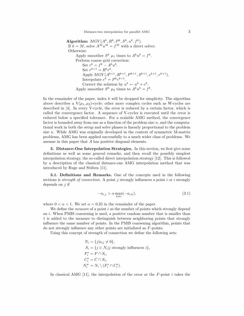
One of the issues is that distance-one interpolation schemes do not treat situationslike the one illustrated in Figure 3.1 correctly. Here we have an F -point with measure
6 De Sterck, Falgout, Nolting, and Yang
smaller than 1 that has no coarse neighbors. This situation can occur for example ifwe have a fairly large strength threshold. Both for classical and direct interpolation,the interpolated error in this point will vanish, and coarse grid correction will not beable to reduce the error in this point.
k i l
Fig. 3.1. Example illustrating a situation occurring with PMIS coarsening, which will notcorrectly be treated by direct or classical interpolation. Black points denote C-points, white pointsdenote F -points, and the arrow from i to l denotes that i strongly depends on l.
A major topic of this paper is to investigate whether distance-two interpolationmethods are able to restore grid-independent convergence to AMG cycles that usePMIS-coarsened grids, without compromising scalability in terms of memory use andexecution time per AMG V-cycle.
4. Long-Range Interpolation Strategies. In this section, various long-distanceinterpolation methods are described. Parallel implementation of some of these interpo-lation methods and parallel scalability results on PMIS-coarsened grids are discussedlater in this paper.
4.1. Multipass Interpolation. Multipass interpolation (‘mp’) is suggested in[12], and is useful for low complexity coarsening algorithms, particularly so-calledaggressive coarsening [12]. We suggested it in [7] as a possible interpolation schemeto fix some of the problems that we saw when using our classical interpolation scheme(3.8). Multipass interpolation proceeds as follows:
1. Use direct interpolation for all F -points i, for which Csi 6= ∅. Place these
points in set F ∗.2. For all i ∈ F \ F ∗ with F ∗ ∩ F s
i 6= 0, replace, in Equation (3.3), for allj ∈ F s
i ∩ F ∗, ej by∑
k∈Cjwjkek, where Cj is the interpolatory set for ej .
Apply direct interpolation to the new equation. Add i to F ∗. Repeat step 2until F ∗ = F .
Multipass interpolation is fairly cheap. However, it is not very powerful, sinceit is based on direct interpolation. If applied to PMIS, it still ends up being directinterpolation for most F -points. However, it fixes the situation illustrated in Figure3.1. If we apply multipass interpolation, the point i will be interpolated by the coarseneighbors (black points) of F -points k and l.
4.2. Jacobi Interpolation. Another approach that remedies convergence is-sues caused by distance-one interpolation formulae is Jacobi interpolation [12]. Thisapproach uses an existing interpolation formula and applies one or more Jacobi it-eration steps to the F -point portion of the interpolation operator leading to a moreaccurate interpolation operator.
Assuming that A and the interpolation operator P (n) are reordered according tothe C/F -splitting and can be written in the following way:
A =
(
AFF AFC
ACF ACC
)
, P (n) =
(
P(n)FC
ICC
)
, (4.1)
then Jacobi iteration on AFF eF +AFCeC = 0, with initial guess e(0)F = P
(0)FCeC , leads
Distance-two interpolation for parallel AMG 7
to
P(n)FC = (IFF −D−1
FF AFF )P(n−1)FC −D−1
FF AFC , (4.2)
where DFF is the diagonal matrix containing the diagonal of AFF , and IFF and ICC
are identity matrices.
If we apply this approach to a distance-one interpolation operator like classi-cal interpolation, we obtain an improved long distance interpolation operator. Thisapproach is also recommended to be used to improve multipass interpolation. Weinclude results where classical interpolation is used followed by one step of Jacobiinterpolation in our numerical experiments and denote them by ‘clas+j’.
4.3. Standard Interpolation. Standard interpolation (‘std’) extends the in-terpolatory set that is used for direct interpolation [12]. This is done by extend-ing the stencil obtained through (3.3) via substitution of every ej with j ∈ F s
i by1/ajj
∑
k∈Njajkek. This leads to the following formula
aiiei +∑
j∈Ni
aijej ≈ 0 (4.3)
with the new neighborhood Ni = Ni ∪⋃
j∈F si
Nj and the new coarse point set Ci =
Ci ∪⋃
j∈F si
Cj . This can greatly increase the size of the interpolatory set.
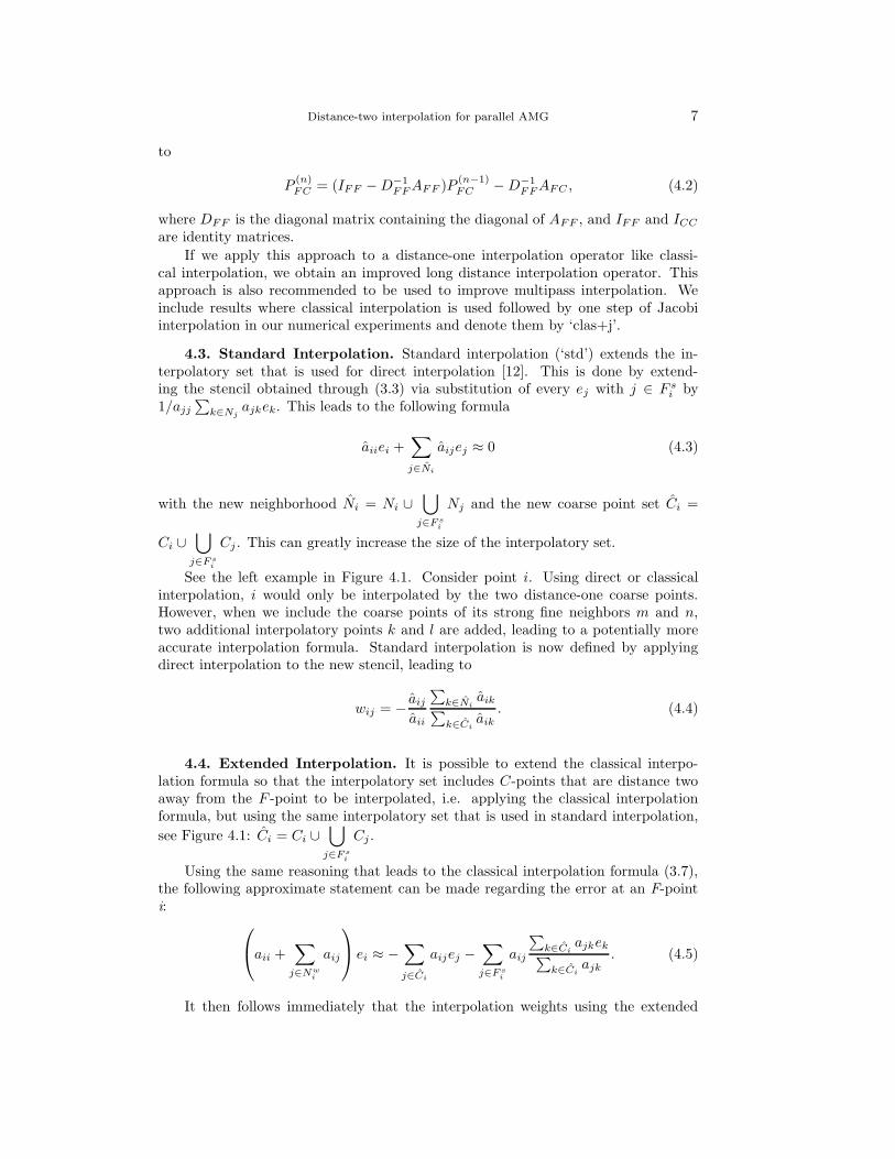
See the left example in Figure 4.1. Consider point i. Using direct or classicalinterpolation, i would only be interpolated by the two distance-one coarse points.However, when we include the coarse points of its strong fine neighbors m and n,two additional interpolatory points k and l are added, leading to a potentially moreaccurate interpolation formula. Standard interpolation is now defined by applyingdirect interpolation to the new stencil, leading to
wij = −aij
aii
∑
k∈Niaik
∑
k∈Ciaik
. (4.4)
4.4. Extended Interpolation. It is possible to extend the classical interpo-lation formula so that the interpolatory set includes C-points that are distance twoaway from the F -point to be interpolated, i.e. applying the classical interpolationformula, but using the same interpolatory set that is used in standard interpolation,
see Figure 4.1: Ci = Ci ∪⋃
j∈F si
Cj .
Using the same reasoning that leads to the classical interpolation formula (3.7),the following approximate statement can be made regarding the error at an F-pointi:
aii +∑
j∈Nwi
aij
ei ≈ −∑
j∈Ci
aijej −∑
j∈F si
aij
∑
k∈Ciajkek
∑
k∈Ciajk
. (4.5)
It then follows immediately that the interpolation weights using the extended

8 De Sterck, Falgout, Nolting, and Yang
k l
n
m
i
i m
n k
l
Fig. 4.1. Example of the interpolatory points for a 5-point stencil (left) and a 9-point stencil(right). The gray point is the point to be interpolated, black points are C-points and white pointsare F -points.
0 2 1 3
-1 -1 -1
2 2
Fig. 4.2. Finite difference 1D Laplace example.
coarse interpolatory set Ci can be defined as
wij = −1
aii +∑
k∈Nwi
aik
aij +∑
k∈F si
aikakj∑
m∈Ci
akm
, j ∈ Ci. (4.6)
This new interpolation formula deals efficiently with strong F − F connectionsthat do not share a common C-point. We call this interpolation strategy ‘extendedinterpolation’ (‘ext’).
4.5. Extended+i Interpolation. While extended interpolation remedies manyproblems that occur with classical interpolation, it does not always lead to the desiredweights. Consider the case given in Figure 4.2. Here we have a 1-dimensional Laplace-problem generated by finite differences. Points 1 and 2 are strongly connected F -points, and points 0 and 3 are coarse points. Clearly 0, 3 is the interpolatory setfor point 1 for the case of extended interpolation. If we apply formula (4.6) to thisexample to calculate w1,0 and w1,3, we obtain
w1,0 = 0.5, w1,3 = 0.5.
This is a better result than we would obtain for direct interpolation (3.5) and classicalinterpolation (3.8):
w1,0 = 1, w1,3 = 0,
Distance-two interpolation for parallel AMG 9
but worse than standard interpolation (4.4), for which we get the intuitively bestinterpolation weights:
w1,0 = 2/3, w1,3 = 1/3. (4.7)
This can be remedied if we include not only connections ajk from strong fineneighbors j of i to points k of the interpolatory set but also connections aji from jto point i itself. An alternative to expression (3.6) for the error in strongly connectedF -points, is then given by
ej ≈
∑
k∈Ci∪i ajkek∑
k∈Ci∪i ajk
. (4.8)
This can be rewritten as
ej ≈
∑
k∈Ciajkek
∑
k∈Ci∪i ajk
+aji ei
∑
k∈Ci∪i ajk
, (4.9)
which then, in a similar way as before, leads to interpolation weights
wij =1
aii
aij +∑
k∈F si
aik
akj∑
l∈Ci∪i akl
, j ∈ Ci, (4.10)
with now
aii = aii +∑
n∈Dwi
ain +∑
k∈F si
aik
aki∑
l∈Ci∪i akl
. (4.11)
We call this modified extended interpolation ‘extended+i’, and refer to it by‘ext+i’ (or sometimes ‘e+i’ to save space) in the tables below. If we apply it to theexample illustrated in Figure 4.2 we obtain weights (4.7).
5. Computational Cost of Interpolation Strategies. In this section we con-sider the cost of some of the interpolation operators described in the previous sections.We use the following notations:
Nc total number of coarse pointsNf total number of fine pointsnk average number of distance-k neighbor pointsck average number of distance-k interpolatory pointsfk average number of strong fine distance-k neighborswk average number of weak distance-k neighborssk average number of common distance-k interpolatory pointsfw average number of strong neighbors treated weakly
Here fw indicates the number of strong F -neighbors that are treated weakly, whichoccur only for classical interpolation (3.7). Also, sk denotes the average number ofC-points which are distance-one neighbors of j ∈ F s
i and also distance-k interpolatorypoints for i, the point to be interpolated. Note that sk is usually smaller than ck andat most equal to ck. Note also that nk = fk + ck + wk.
10 De Sterck, Falgout, Nolting, and Yang
In our considerations we assume a compressed sparse row data format, i.e. threearrays are used to store the matrix: a real array that contains the coefficients of thematrix, an integer array that contains the column indices for each coefficient and aninteger array that contains pointers to the beginning of each row for the other twoarrays. We also assume an additional integer array which indicates whether a pointis an F - or a C-point.
For all interpolation operators mentioned before, it is necessary to determine atfirst the interpolatory set. At the same time the data structure for the interpolationoperator can be determined. This can be accomplished by sweeping through each rowthat belongs to an F -point: coarse neighbors are identified via integer comparisons,and the pointer array for the interpolation operator is generated. For the distance-twointerpolation schemes, it is also necessary to check neighbors of strong fine neighbors.This requires n1 comparisons for direct and classical interpolation, and (f1 + 1)n1
comparisons for extended, extended+i and standard interpolation. The final datastructure contains Nc + Nfc1 coefficients for classical and direct interpolation, andNc + Nf (c1 + c2) coefficients for extended(+i) and standard interpolation.
Next, the interpolation data structure is filled.For direct interpolation, all that is required is to sweep through a whole row
once to compute αi = −∑
k∈Niaik/
(
aii
∑
k∈Csiaik
)
and then multiply the relevant
matrix elements aij with αi. The sum in the denominator requires an additional n1
comparisons, and the two summations require n1 + 1 additions.For classical, extended and extended+i interpolation one needs to first compute
for each point k ∈ F si \ F s∗
i , αik = aik/(
∑
m∈Dsiakm
)
with the appropriate set Dsi ,
which is different for each operator. For example, for classical interpolation, thisrequires f1n1 comparisons. After this step, all these coefficients need to be processedagain in order to add αijakj to the appropriate weights. This requires an additionalf1n1 comparisons. The number of additions, multiplications and divisions can bedetermined similarly.
For standard interpolation, at first the new stencil needs to be computed, leadingto f1n1 additions and multiplications. After this one proceeds just as for directinterpolation with a much larger stencil of size n1 + n2.
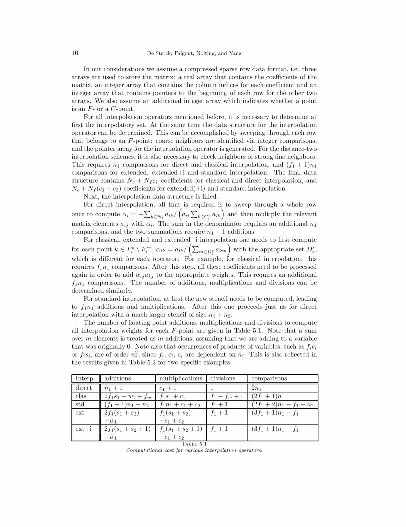
The number of floating point additions, multiplications and divisions to computeall interpolation weights for each F -point are given in Table 5.1. Note that a sumover m elements is treated as m additions, assuming that we are adding to a variablethat was originally 0. Note also that occurrences of products of variables, such as fici
or fisi, are of order n2i , since fi, ci, si are dependent on ni. This is also reflected in
the results given in Table 5.2 for two specific examples.
Interp. additions multiplications divisions comparisons
direct n1 + 1 c1 + 1 1 2n1
clas 2f1s1 + w1 + fw f1s1 + c1 f1 − fw + 1 (2f1 + 1)n1
std (f1 + 1)n1 + n2 f1n1 + c1 + c2 f1 + 1 (2f1 + 2)n1 − f1 + n2
ext 2f1(s1 + s2) f1(s1 + s2) f1 + 1 (3f1 + 1)n1 − f1
+w1 +c1 + c2
ext+i 2f1(s1 + s2 + 1) f1(s1 + s2 + 1) f1 + 1 (3f1 + 1)n1 − f1
+w1 +c1 + c2
Table 5.1
Computational cost for various interpolation operators.

Distance-two interpolation for parallel AMG 11
Let us look at some examples to get an idea about the actual cost involved. Firstconsider a 5-point stencil as in Figure 4.1. Here, we have the following parameters:c1 = f1 = 2, w1 = w2 = 0, n1 = 4, fw = 2, s1 = 0, c2 = 2, f2 = 3, n2 =5, s2 = 1.5. Table 5.2 shows the resulting interpolation cost. Next, we look at anexample with a bigger stencil, see Figure 4.1 and Table 5.2. The parameters are nowc1 = 2, f1 = 6, w1 = w2 = 0, n1 = 8, fw = 1, s1 = 1, c2 = 3, f2 = 12, n2 =15, s2 = 1. We clearly see that a larger stencil significantly increases the ratio ofclassical over direct interpolation, as well as that of distance-two over distance-oneinterpolations.
Left example in Fig. 4.1 Right example in Fig. 4.1Interpol. adds mults divs comps adds mults divs comps
direct 5 3 1 8 9 3 1 16clas 2 2 1 20 13 8 6 104std 17 12 3 19 71 53 7 73ext 6 7 3 26 24 17 7 146ext+i 10 9 3 26 36 23 7 146
Table 5.2
Cost for examples in Figure 4.1.
Table 5.3 shows the times for calculating these interpolation operators for matriceswith stencils of various sizes. Two two-dimensional examples, one with a 5-pointand one with a 9-point stencil, were examined on a 1000 × 1000 grid. The three-dimensional examples, with a 7-point and a 27-point stencil, were examined for an80× 80× 80 grid. We have also included actual measurements of the average numberof interpolatory points for these examples. As expected, larger stencils lead to a largernumber of operations for each interpolation operator, with a much more significantincrease for distance-two interpolation operators, particularly for the 3-dimensionalproblems. These effects are significant, especially since on coarser levels the stencilsbecome larger and, thus, impact the total setup time.
InterpolationStencil c1 c2 direct clas std ext ext+i
5-pt 2.3 1.9 0.27 0.35 0.64 0.51 0.549-pt 1.8 2.8 0.36 1.11 2.16 2.09 2.48
7-pt 2.7 4.1 0.19 0.31 0.80 0.73 0.8127-pt 2.3 7.2 0.40 3.72 8.00 7.43 8.32
Table 5.3
Average number of distance-one (c1) and distance-two (c2) interpolatory points and times forvarious interpolation operators.
6. Sequential Numerical Results. While the previous section examined thecomputational cost for the interpolation operator, we are of course mainly interested inthe performance of the complete solver, which also includes coarsening, the generationof the coarse grid operator as well as the solve phase. We apply the new and oldinterpolation operators here to a variety of test problems from [7] to compare theirefficiency. We did not include results using direct interpolation, since it performsworse than classical and multipass interpolation for the problems considered, nor
12 De Sterck, Falgout, Nolting, and Yang
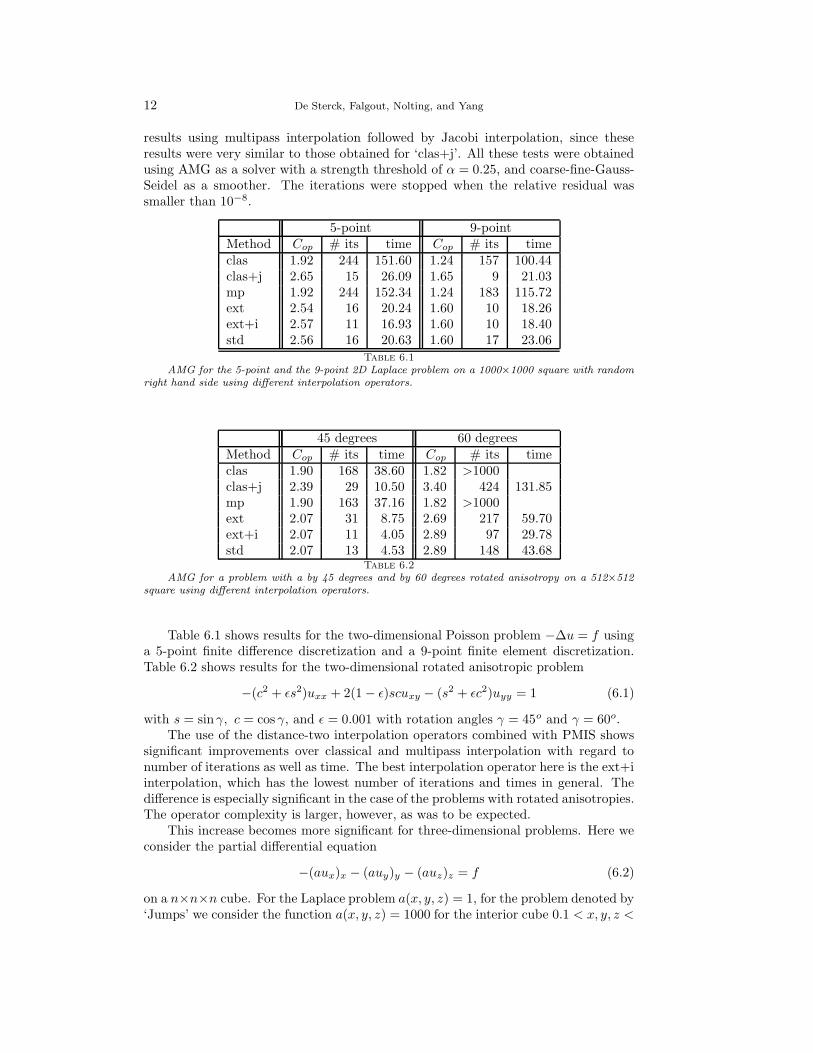
results using multipass interpolation followed by Jacobi interpolation, since theseresults were very similar to those obtained for ‘clas+j’. All these tests were obtainedusing AMG as a solver with a strength threshold of α = 0.25, and coarse-fine-Gauss-Seidel as a smoother. The iterations were stopped when the relative residual wassmaller than 10−8.
5-point 9-pointMethod Cop # its time Cop # its timeclas 1.92 244 151.60 1.24 157 100.44clas+j 2.65 15 26.09 1.65 9 21.03mp 1.92 244 152.34 1.24 183 115.72ext 2.54 16 20.24 1.60 10 18.26ext+i 2.57 11 16.93 1.60 10 18.40std 2.56 16 20.63 1.60 17 23.06
Table 6.1
AMG for the 5-point and the 9-point 2D Laplace problem on a 1000×1000 square with randomright hand side using different interpolation operators.
45 degrees 60 degreesMethod Cop # its time Cop # its timeclas 1.90 168 38.60 1.82 >1000clas+j 2.39 29 10.50 3.40 424 131.85mp 1.90 163 37.16 1.82 >1000ext 2.07 31 8.75 2.69 217 59.70ext+i 2.07 11 4.05 2.89 97 29.78std 2.07 13 4.53 2.89 148 43.68
Table 6.2
AMG for a problem with a by 45 degrees and by 60 degrees rotated anisotropy on a 512×512square using different interpolation operators.
Table 6.1 shows results for the two-dimensional Poisson problem −∆u = f usinga 5-point finite difference discretization and a 9-point finite element discretization.Table 6.2 shows results for the two-dimensional rotated anisotropic problem
−(c2 + εs2)uxx + 2(1− ε)scuxy − (s2 + εc2)uyy = 1 (6.1)
with s = sin γ, c = cos γ, and ε = 0.001 with rotation angles γ = 45o and γ = 60o.The use of the distance-two interpolation operators combined with PMIS shows
significant improvements over classical and multipass interpolation with regard tonumber of iterations as well as time. The best interpolation operator here is the ext+iinterpolation, which has the lowest number of iterations and times in general. Thedifference is especially significant in the case of the problems with rotated anisotropies.The operator complexity is larger, however, as was to be expected.
This increase becomes more significant for three-dimensional problems. Here weconsider the partial differential equation
−(aux)x − (auy)y − (auz)z = f (6.2)
on a n×n×n cube. For the Laplace problem a(x, y, z) = 1, for the problem denoted by‘Jumps’ we consider the function a(x, y, z) = 1000 for the interior cube 0.1 < x, y, z <

Distance-two interpolation for parallel AMG 13
7-point 27-point JumpsMethod Cop # its time Cop # its time Cop # its timeclas 2.34 45 10.21 1.09 28 10.58 2.50 >1000clas+j 5.12 11 20.35 1.34 8 17.10 5.37 15 20.99mp 2.35 47 10.40 1.10 30 9.39 2.50 80 17.37ext 4.93 11 16.70 1.35 8 21.32 5.27 15 16.89ext+i 4.27 9 14.48 1.35 8 21.55 5.10 11 15.96std 4.20 10 12.78 1.38 10 18.58 5.21 18 17.47
Table 6.3
AMG for a 7-point 3D Laplace problem, a problem with a 27-point stencil and a 3D structuredPDE problem with jumps on a 60 × 60 × 60 cube with a random right hand side using differentinterpolation operators.
0.9, a(x, y, z) = 0.01 for 0 < x, y, z < 0.1 and the other cubes of size 0.1× 0.1× 0.1that are located at the corners of the unit cube and a(x, y, z) = 1 elsewhere. The27-point problem is a matrix with a 27-point stencil with the value 26 in the interiorand -1 elsewhere and is being tested because we also wanted to consider a problemwith a larger stencil.
While for these problems AMG convergence factors for distance-two interpolationimprove significantly compared to classical and multipass interpolation, as can beseen in Table 6.3, overall times are worse for the 7pt 3D Laplace problem as well asthe 27-point problem on a 60 × 60 × 60 grid. The only problem on the 60 × 60 ×60 grid that benefits from distance-two interpolation operators also with regard totime is the problem with jumps, which requires long-distance interpolation to evenconverge. Using distance-two interpolation operators leads to complexities abouttwice as large as those obtained when using classical or multi-pass interpolation,which work relatively well for the 7- and 27-point problem on the 60× 60× 60 grid.However, when we scale up the problem sizes, they show very good scalability interms of AMG convergence factors, as can be seen in Figure 6.1, which shows thenumber of iterations for a 3D 7-pt Laplace problem on a n×n×n grid for increasingn. The anticipated large differences in numbers of iterations between distance-oneand distance-two interpolations show up in the 2D results of Tables 6.1 and 6.2 ongrids with 1000 points per direction, but are not particularly significant yet in the 3Dresults of Table 6.3 with only 60 points per direction. It is expected, however, thatfor the large problems that we want to solve on a parallel computer, distance-twointerpolation operators will lead to overall better times than classical or multi-passinterpolation due to scalable AMG convergence factors, if the operator complexitycan be kept under control. See Section 9 for actual test results.
7. Reducing Operator Complexity. While the methods described in the pre-vious section largely restore grid-independent convergence to AMG cycles that usePMIS-coarsened grids, they also lead to much larger operator complexities for theV-cycles. Therefore, it is necessary to consider ways to reduce these complexitieswhile (hopefully) retaining the improved convergence. In this section we describe afew ways of achieving this.
7.1. Choosing Smaller Interpolatory Sets. It is certainly possible to con-sider other interpolatory sets, which are larger than Cs
i , but smaller than Ci. Par-ticularly, it appears that a good interpolatory set would be one that only extends Cs
i
for strong F − F connections without a common C-point, since in the other cases

14 De Sterck, Falgout, Nolting, and Yang
0
10
20
30
40
50
60
70
20 40 60 80 100
n
no
. of
its.
clas
mp
clas+j
std
ext
ext+i
Fig. 6.1. Number of iterations for PMIS with various interpolation operators for a 3D 7-pointLaplace problem on a n × n × n-grid.
point i is likely already surrounded by interpolatory points and an extension is notnecessary. If we look at the right example in Figure 4.1, we see that neighbor k of i isthe only fine neighbor that does not share a C-point with i. Consequently, it may besufficient to only include points n and l in the extended interpolatory set. Applyingthis approach to the extended interpolation leads to so-called F −F interpolation [3].The size of the interpolatory set can be further decreased if we limit the number ofC-points added when an F -point is encountered that does not have common coarseneighbors. This has been done in the so-called F − F1 interpolation [3], where onlythe first C-point is added. For the right example in Figure 4.1 this means that onlypoint n or point l would be added to the interpolatory set for i.
Choosing a smaller interpolatory set decreases c2 and with it s2, leading to fewermultiplications and additions for the extended interpolation methods. On the otherhand, additional operations are needed to determine which coarse neighbors of strongF -points are common C-points. This means that the actual determination of theinterpolation operator might not be faster than creating the extended interpolationoperators. The real benefit, however, is achieved by the fact that the use of smallerinterpolatory sets leads to smaller stencils for the coarse grid operator and hence tosmaller overall operator complexities.
Applying these methods to some of our previous test problems, we get the resultsshown in Tables 7.1 and 7.2. Here, ‘x-cc’ denotes that interpolation ‘x’ is used, butthe interpolatory set is only extended when there are no common C-points. Similarly,‘x-ccs’ is just like ‘x-cc’, except that for every strong F -point without a commonC-point only a single C-point is added.
The results show that 2-dimensional problems do not benefit from this strategy,since operator complexities are only slightly decreased, while the number of iterationsincreases. Therefore total times increase. However, 3-dimensional problems can besolved much faster due to significantly decreased setup times leading to only halfthe total times when the ‘ccs’-strategy is employed. Again, these beneficial effectsare expected to be stronger on larger grids. Indeed, additional numerical tests (notpresented here, see [3]) also show that the ‘x-cc’ and ‘x-ccs’ distance-two interpolationsresult in algorithms that are highly scalable as a function of problem size: Cop tends
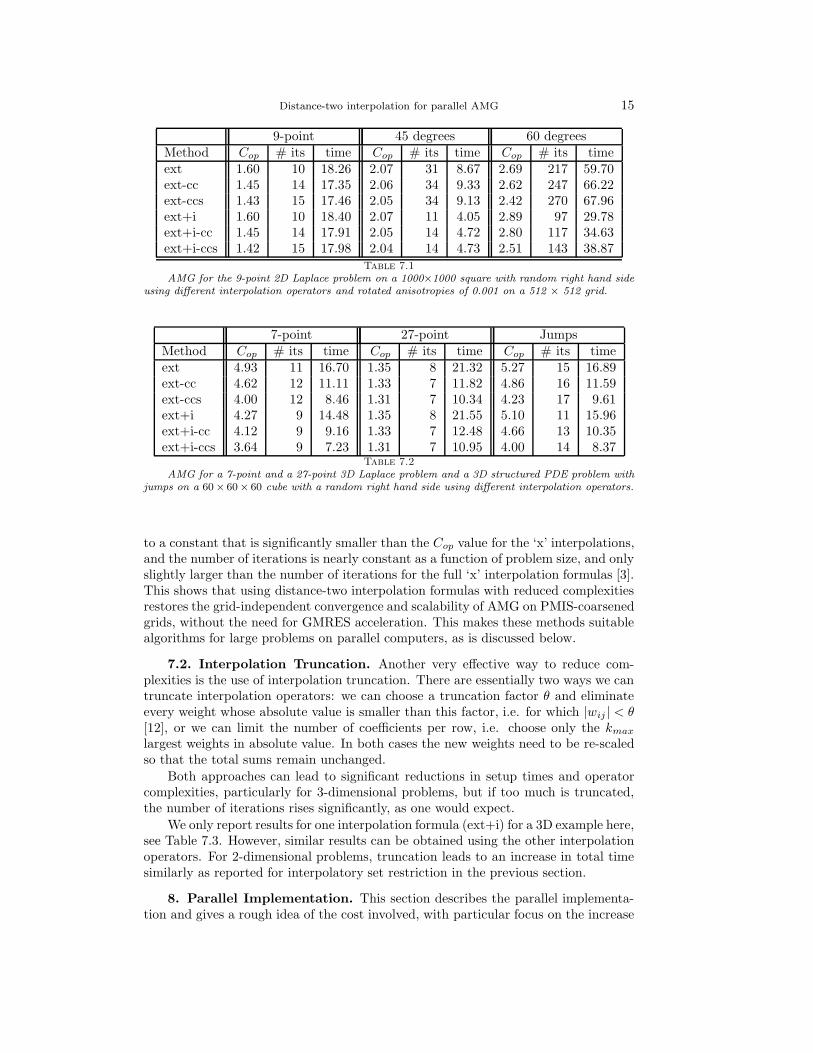
Distance-two interpolation for parallel AMG 15
9-point 45 degrees 60 degreesMethod Cop # its time Cop # its time Cop # its timeext 1.60 10 18.26 2.07 31 8.67 2.69 217 59.70ext-cc 1.45 14 17.35 2.06 34 9.33 2.62 247 66.22ext-ccs 1.43 15 17.46 2.05 34 9.13 2.42 270 67.96ext+i 1.60 10 18.40 2.07 11 4.05 2.89 97 29.78ext+i-cc 1.45 14 17.91 2.05 14 4.72 2.80 117 34.63ext+i-ccs 1.42 15 17.98 2.04 14 4.73 2.51 143 38.87
Table 7.1
AMG for the 9-point 2D Laplace problem on a 1000×1000 square with random right hand sideusing different interpolation operators and rotated anisotropies of 0.001 on a 512 × 512 grid.
7-point 27-point JumpsMethod Cop # its time Cop # its time Cop # its timeext 4.93 11 16.70 1.35 8 21.32 5.27 15 16.89ext-cc 4.62 12 11.11 1.33 7 11.82 4.86 16 11.59ext-ccs 4.00 12 8.46 1.31 7 10.34 4.23 17 9.61ext+i 4.27 9 14.48 1.35 8 21.55 5.10 11 15.96ext+i-cc 4.12 9 9.16 1.33 7 12.48 4.66 13 10.35ext+i-ccs 3.64 9 7.23 1.31 7 10.95 4.00 14 8.37
Table 7.2
AMG for a 7-point and a 27-point 3D Laplace problem and a 3D structured PDE problem withjumps on a 60× 60× 60 cube with a random right hand side using different interpolation operators.
to a constant that is significantly smaller than the Cop value for the ‘x’ interpolations,and the number of iterations is nearly constant as a function of problem size, and onlyslightly larger than the number of iterations for the full ‘x’ interpolation formulas [3].This shows that using distance-two interpolation formulas with reduced complexitiesrestores the grid-independent convergence and scalability of AMG on PMIS-coarsenedgrids, without the need for GMRES acceleration. This makes these methods suitablealgorithms for large problems on parallel computers, as is discussed below.
7.2. Interpolation Truncation. Another very effective way to reduce com-plexities is the use of interpolation truncation. There are essentially two ways we cantruncate interpolation operators: we can choose a truncation factor θ and eliminateevery weight whose absolute value is smaller than this factor, i.e. for which |wij | < θ[12], or we can limit the number of coefficients per row, i.e. choose only the kmax
largest weights in absolute value. In both cases the new weights need to be re-scaledso that the total sums remain unchanged.
Both approaches can lead to significant reductions in setup times and operatorcomplexities, particularly for 3-dimensional problems, but if too much is truncated,the number of iterations rises significantly, as one would expect.
We only report results for one interpolation formula (ext+i) for a 3D example here,see Table 7.3. However, similar results can be obtained using the other interpolationoperators. For 2-dimensional problems, truncation leads to an increase in total timesimilarly as reported for interpolatory set restriction in the previous section.
8. Parallel Implementation. This section describes the parallel implementa-tion and gives a rough idea of the cost involved, with particular focus on the increase

16 De Sterck, Falgout, Nolting, and Yang
truncation factor max.# of weightsθ Cop # its time kmax Cop # its time0 4.27 9 14.48
0.1 4.13 9 10.72 7 3.75 9 8.630.2 3.88 9 8.52 6 3.42 9 7.410.3 3.39 10 6.82 5 3.01 10 6.420.4 3.02 13 6.60 4 2.73 14 6.300.5 2.75 20 7.67 3 2.48 24 7.41
Table 7.3
Effect of truncation on AMG with ext+i interpolation for a 7-point 3D Laplace problem on a60× 60 × 60 cube with a random right hand side. (Note that ‘ass’ denotes the average stencil size.)
in communication required for the distance-two interpolation formulae compared todistance-one interpolation. Since the core computation for the interpolation routinesis approximately the same as in the sequential case, we only focus on the additionalcomputations that are required for inter-communication between processors.
In parallel, each matrix is stored using a parallel data format, the ParCSR ma-trix data structure, which is described and analyzed in detail in [8]. Matrices aredistributed across processors by contiguous blocks of rows, which are stored via twocompressed sparse row matrices, one storing the local entries and the other one storingthe off-processor entries. There is an additional array containing a mapping for theoff-processor neighbor points. The data structure also contains the information nec-essary to retrieve information from distance-one off-processor neighbors. It howeverdoes not contain information on off-processor distance-two neighbors, which com-plicates the parallel implementation of distance-two interpolation operators. Whendetermining these neighbors, there are four scenarios that need to be considered, seeFigure 8.1. Consider point i, which is the point to be interpolated to, and is residingon Processor 0. A distance-two neighbor can reside on the same processor as i, likepoint j; it can be a distance-one neighbor to another point on Proc. 0, like pointl, and therefore be already contained in the off-processor mapping; it can be a newpoint on a neighbor processor, like point k, or it can be located on a processor, whichis currently not a neighbor processor to Proc. 0, like point m.
i
j
k
m l
Proc. 0 Proc. 1
Proc. 2
Proc. 3
Fig. 8.1. Example of off-processor distance-two neighbors of point i. Black points are C-points,and white points are F -points.
There are basically five additional parts that are required for the parallel im-plementation, and for which we give rough estimates of the cost involved below.
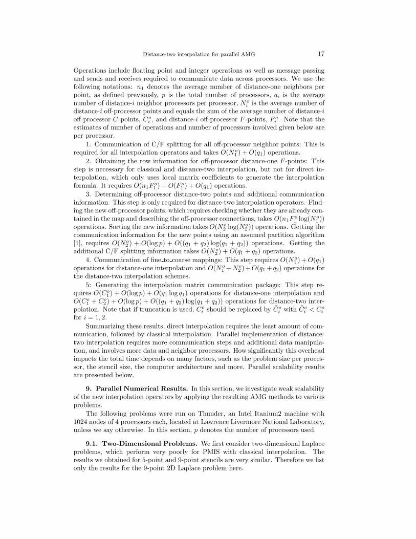
Distance-two interpolation for parallel AMG 17
Operations include floating point and integer operations as well as message passingand sends and receives required to communicate data across processors. We use thefollowing notations: n1 denotes the average number of distance-one neighbors perpoint, as defined previously, p is the total number of processors, qi is the averagenumber of distance-i neighbor processors per processor, N o
i is the average number ofdistance-i off-processor points and equals the sum of the average number of distance-ioff-processor C-points, Co
i , and distance-i off-processor F -points, F oi . Note that the
estimates of number of operations and number of processors involved given below areper processor.
1. Communication of C/F splitting for all off-processor neighbor points: This isrequired for all interpolation operators and takes O(N o
1 ) + O(q1) operations.
2. Obtaining the row information for off-processor distance-one F -points: Thisstep is necessary for classical and distance-two interpolation, but not for direct in-terpolation, which only uses local matrix coefficients to generate the interpolationformula. It requires O(n1F
o1 ) + O(F o
1 ) + O(q1) operations.
3. Determining off-processor distance-two points and additional communicationinformation: This step is only required for distance-two interpolation operators. Find-ing the new off-processor points, which requires checking whether they are already con-tained in the map and describing the off-processor connections, takes O(n1F
o1 log(No
1 ))operations. Sorting the new information takes O(N o
2 log(No2 )) operations. Getting the
communication information for the new points using an assumed partition algorithm[1], requires O(No
2 ) + O(log p) + O((q1 + q2) log(q1 + q2)) operations. Getting theadditional C/F splitting information takes O(N o
2 ) + O(q1 + q2) operations.
4. Communication of fine to coarse mappings: This step requires O(N o1 ) + O(q1)
operations for distance-one interpolation and O(N o1 +No
2 )+O(q1 + q2) operations forthe distance-two interpolation schemes.
5: Generating the interpolation matrix communication package: This step re-quires O(Co
1 ) + O(log p) + O(q1 log q1) operations for distance-one interpolation andO(Co
1 + Co2 ) + O(log p) + O((q1 + q2) log(q1 + q2)) operations for distance-two inter-
polation. Note that if truncation is used, Coi should be replaced by Co
i with Coi < Co
i
for i = 1, 2.
Summarizing these results, direct interpolation requires the least amount of com-munication, followed by classical interpolation. Parallel implementation of distance-two interpolation requires more communication steps and additional data manipula-tion, and involves more data and neighbor processors. How significantly this overheadimpacts the total time depends on many factors, such as the problem size per proces-sor, the stencil size, the computer architecture and more. Parallel scalability resultsare presented below.
9. Parallel Numerical Results. In this section, we investigate weak scalabilityof the new interpolation operators by applying the resulting AMG methods to variousproblems.
The following problems were run on Thunder, an Intel Itanium2 machine with1024 nodes of 4 processors each, located at Lawrence Livermore National Laboratory,unless we say otherwise. In this section, p denotes the number of processors used.
9.1. Two-Dimensional Problems. We first consider two-dimensional Laplaceproblems, which perform very poorly for PMIS with classical interpolation. Theresults we obtained for 5-point and 9-point stencils are very similar. Therefore we listonly the results for the 9-point 2D Laplace problem here.
18 De Sterck, Falgout, Nolting, and Yang
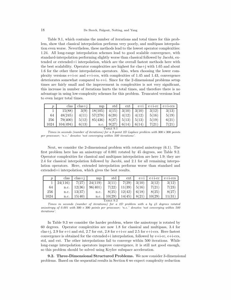
Table 9.1, which contains the number of iterations and total times for this prob-lem, show that classical interpolation performs very poorly, and multipass interpola-tion even worse. Nevertheless, these methods lead to the lowest operator complexities:1.24. All long-range interpolation schemes lead to good scalable convergence, withstandard-interpolation performing slightly worse than classical followed by Jacobi, ex-tended or extended+i interpolation, which are the overall fastest methods here withthe best scalability. Operator complexities are highest for clas+j with 1.65 and about1.6 for the other three interpolation operators. Also, when choosing the lower com-plexity versions e+i-cc and e+i-ccs, with complexities of 1.45 and 1.43, convergencedeteriorates somewhat compared to e+i. Since for the 2-dimensional problems setuptimes are fairly small and the improvement in complexities is not very significant,this increase in number of iterations hurts the total times, and therefore there is noadvantage in using low-complexity schemes for this problem. Truncated versions leadto even larger total times.
p clas clas+j mp std ext e+i e+i-cc e+i-ccs1 15(88) 3(9) 18(105) 4(15) 3(10) 3(10) 3(12) 3(13)
64 48(245) 4(11) 57(278) 6(20) 4(12) 4(12) 5(16) 5(19)256 79(400) 5(12) 85(436) 8(27) 5(13) 5(13) 5(19) 6(21)
1024 104(494) 6(13) n.c. 9(27) 6(14) 6(14) 7(21) 7(21)Table 9.1
Times in seconds (number of iterations) for a 9-point 2D Laplace problem with 300×300 pointsper processor; ‘n.c.’ denotes ‘not converging within 500 iterations’.
Next, we consider the 2-dimensional problem with rotated anisotropy (6.1). Thefirst problem here has an anisotropy of 0.001 rotated by 45 degrees, see Table 9.2.Operator complexities for classical and multipass interpolation are here 1.9; they are2.4 for classical interpolation followed by Jacobi, and 2.1 for all remaining interpo-lation operators. Here, extended interpolation performs worse than standard andextended+i interpolation, which gives the best results.
p clas clas+j mp std ext e+i e+i-cc e+i-ccs1 24(116) 7(27) 24(119) 3(11) 7(29) 3(10) 3(12) 3(12)
64 n.c. 12(36) 96(401) 7(22) 11(39) 5(16) 7(21) 7(23)256 n.c. 13(37) n.c. 8(25) 12(42) 6(18) 8(25) 8(27)
1024 n.c. 15(40) n.c. 10(29) 14(45) 8(21) 10(29) 11(31)Table 9.2
Times in seconds (number of iterations) for a 2D problem with a by 45 degrees rotatedanisotropy of 0.001 with 300 × 300 points per processor; ‘n.c.’ denotes ‘not converging within 500iterations’.
In Table 9.3 we consider the harder problem, where the anisotropy is rotated by60 degrees. Operator complexities are now 1.8 for classical and multipass, 3.4 forclas+j, 2.9 for e+i and std, 2.7 for ext, 2.8 for e+i-cc and 2.5 for e+i-ccs. Here fastestconvergence is obtained for the extended+i interpolation, followed by e+i-cc, e+i-ccs,std, and ext. The other interpolations fail to converge within 500 iterations. Whilelong-range interpolation operators improve convergence, it is still not good enough,so this problem should be solved using Krylov subspace acceleration.
9.2. Three-Dimensional Structured Problems. We now consider 3-dimensionalproblems. Based on the sequential results in Section 6 we expect complexity reduction
Distance-two interpolation for parallel AMG 19
p clas clas+j mp std ext e+i e+i-cc e+i-ccs1 n.c. 105(342) n.c. 30(107) 45(172) 22(79) 24(87) 28(112)
64 n.c. n.c. n.c. 79(256) 96(330) 47(152) 59(196) 70(254)256 n.c. n.c. n.c. 95(305) 110(374) 56(176) 70(227) 84(299)
1024 n.c. n.c. n.c. 113(357) 123(408) 62(193) 82(263) 100(347)Table 9.3
Times in seconds (number of iterations) for a 2D problem with a by 60 degrees rotatedanisotropy of 0.001 with 300 × 300 points per processor; ‘n.c.’ denotes ‘not converging within 500iterations’.
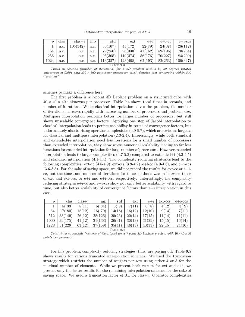
schemes to make a difference here.The first problem is a 7-point 3D Laplace problem on a structured cube with
40 × 40 × 40 unknowns per processor. Table 9.4 shows total times in seconds, andnumber of iterations. While classical interpolation solves the problem, the numberof iterations increases rapidly with increasing number of processors and problem size.Multipass interpolation performs better for larger number of processors, but stillshows unscalable convergence factors. Applying one step of Jacobi interpolation toclassical interpolation leads to perfect scalability in terms of convergence factors, butunfortunately also to rising operator complexities (4.9-5.7), which are twice as large asfor classical and multipass interpolation (2.3-2.4). Interestingly, while both standardand extended+i interpolation need less iterations for a small number of processorsthan extended interpolation, they show worse numerical scalability leading to far lessiterations for extended interpolation for large number of processors. However extendedinterpolation leads to larger complexities (4.7-5.3) compared to extended+i (4.2-4.5)and standard interpolation (4.1-4.4). The complexity reducing strategies lead to thefollowing complexities: ext-cc (4.5-4.9), ext-ccs (3.9-4.2), e+i-cc (4.0-4.3), and e+i-ccs(3.6-3.8). For the sake of saving space, we did not record the results for ext-cc or e+i-cc, but the times and number of iterations for these methods was in between thoseof ext and ext-ccs, or e+i and e+i-ccs, respectively. Interestingly, the complexityreducing strategies e+i-cc and e+i-ccs show not only better scalability with regard totime, but also better scalability of convergence factors than e+i interpolation in thiscase.
p clas clas+j mp std ext e+i ext-ccs e+i-ccs1 5( 33) 8(11) 6( 34) 5( 9) 7(11) 6( 8) 4(12) 3( 9)
64 17( 80) 18(12) 16( 79) 14(18) 16(12) 12(10) 9(14) 7(11)512 33(149) 26(12) 28(126) 20(26) 20(14) 17(15) 11(14) 11(11)
1000 39(175) 41(12) 31(138) 26(31) 30(13) 31(39) 15(15) 16(14)1728 51(229) 63(12) 37(159) 35(41) 46(13) 40(33) 22(15) 24(16)
Table 9.4
Total times in seconds (number of iterations) for a 7 point 3D Laplace problem with 40×40×40points per processor.
For this problem, complexity reducing strategies, thus, are paying off. Table 9.5shows results for various truncated interpolation schemes. We used the truncationstrategy which restricts the number of weights per row using either 4 or 5 for themaximal number of elements. While we present both results for ext and e+i, wepresent only the faster results for the remaining interpolation schemes for the sake ofsaving space. We used a truncation factor of 0.1 for clas+j. Operator complexities

20 De Sterck, Falgout, Nolting, and Yang
p ext4 ext5 e+i4 e+i5 ext-cc5 e+i-cc5 std5 clas+j0.11 3(13) 3(11) 3(12) 3(9) 3(11) 3(9) 4(12) 3(13)
64 6(19) 7(15) 7(19) 7(13) 6(14) 6(13) 9(25) 9(23)512 9(25) 8(18) 11(28) 10(19) 8(17) 8(17) 15(39) 13(36)
1000 10(25) 11(18) 11(30) 12(20) 10(18) 9(17) 17(39) 15(37)1728 12(29) 12(21) 13(35) 14(24) 11(21) 11(20) 28(46) 19(45)
Table 9.5
Total times in seconds (number of iterations) for a 7 point 3D Laplace problem with 40×40×40points per processor.
were fairly consistent here across increasing numbers of processors: we obtained 2.9for ext4, 3.2 for ext5, 2.8 for e+i4, 3.1 for e+i5, 3.2 for ext-cc5, 3.1 for e+i-cc5, 3.2for std5 and 3.0 for clas+j0.1. Clearly, using four compared to five weights leads tolower complexities, but larger number of iterations. Total times are not significantlydifferent. Comparing the fastest method, e+i-cc5, on 1728 processors to PMIS withclassical interpolation, we see a factor of 11 in improvement with regard to numberof iterations and a factor of 5 in improvement with regard to total time with a slightincrease in complexity.
Table 9.6 shows results for the problem with jumps (6.2), for which PMIS withclassical interpolation was shown to completely fail. Multipass interpolation convergeshere with highly degrading scalability but good complexities of 2.4. Applying Jacobiinterpolation to classical interpolation leads to very good convergence, but, due tooperator complexities between 5.1 and 5.7, it leads to a much more expensive setupand solve cycle. Applying a truncation factor of 0.1 as in the previous example leads toextremely bad convergence and is not helpful here. Standard interpolation convergesvery well for small number of processors, but diverges if p is greater or equal to 64.Interestingly enough std4 converges, albeit not very well.
p mp clas+j ext e+i ext-ccs e+i-ccs std4 ext-cc51 11( 64) 8(14) 7(14) 6(10) 5(18) 4(15) 6( 26) 5(17)
64 35(176) 20(17) 17(17) 15(14) 11(21) 9(19) 18( 71) 11(24)512 58(280) 31(20) 24(24) 21(20) 15(24) 13(21) 27( 98) 11(30)
1000 65(306) 35(21) 27(20) 26(21) 19(24) 18(22) 33(113) 14(33)1728 77(350) 60(21) 73(70) 43(26) 25(29) 29(23) 53(169) 17(36)
Table 9.6
Total times in seconds (number of iterations) for a structured 3D problem with jumps with40 × 40 × 40 points per processor.
9.3. Unstructured Problems. In this section, we consider various linear sys-tems on unstructured grids that have been generated by finite element discretizations.All of these problems were run on an Intel Xeon Linux cluster at Lawrence LivermoreNational Laboratory. The first problem is the three-dimensional diffusion problem−a1(x, y, z)uxx − a2(x, y, z)uyy − a3(x, y, z)uzz = f with Dirichlet boundary condi-tions on an unstructured cube. The material properties are discontinuous, and thereare approximately 90,000 degrees of freedom per processor. See Figure 9.1 for anillustration of the grid used. There are five regions: four layers and the thin stickin the middle of the domain. This grid is further refined when larger number ofprocessors are used. The functions ai(x, y, z), i = 1, 2, 3 are constant within each of
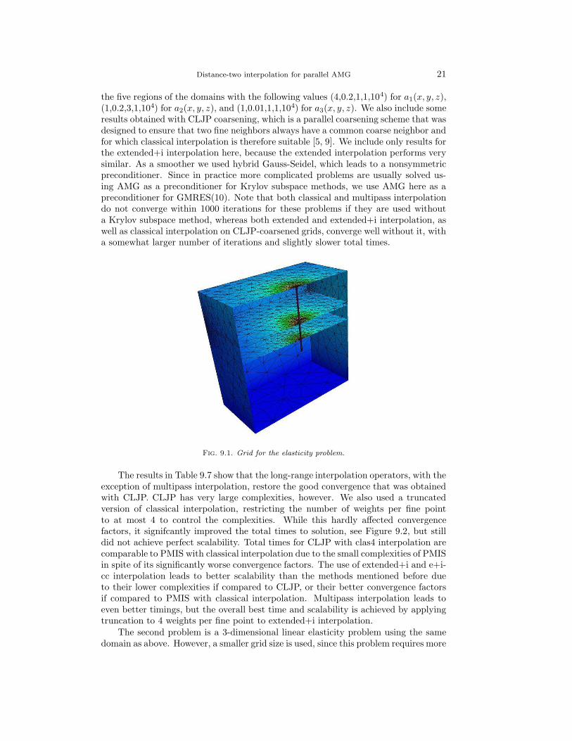
Distance-two interpolation for parallel AMG 21
the five regions of the domains with the following values (4,0.2,1,1,104) for a1(x, y, z),(1,0.2,3,1,104) for a2(x, y, z), and (1,0.01,1,1,104) for a3(x, y, z). We also include someresults obtained with CLJP coarsening, which is a parallel coarsening scheme that wasdesigned to ensure that two fine neighbors always have a common coarse neighbor andfor which classical interpolation is therefore suitable [5, 9]. We include only results forthe extended+i interpolation here, because the extended interpolation performs verysimilar. As a smoother we used hybrid Gauss-Seidel, which leads to a nonsymmetricpreconditioner. Since in practice more complicated problems are usually solved us-ing AMG as a preconditioner for Krylov subspace methods, we use AMG here as apreconditioner for GMRES(10). Note that both classical and multipass interpolationdo not converge within 1000 iterations for these problems if they are used withouta Krylov subspace method, whereas both extended and extended+i interpolation, aswell as classical interpolation on CLJP-coarsened grids, converge well without it, witha somewhat larger number of iterations and slightly slower total times.
Fig. 9.1. Grid for the elasticity problem.
The results in Table 9.7 show that the long-range interpolation operators, with theexception of multipass interpolation, restore the good convergence that was obtainedwith CLJP. CLJP has very large complexities, however. We also used a truncatedversion of classical interpolation, restricting the number of weights per fine pointto at most 4 to control the complexities. While this hardly affected convergencefactors, it signifcantly improved the total times to solution, see Figure 9.2, but stilldid not achieve perfect scalability. Total times for CLJP with clas4 interpolation arecomparable to PMIS with classical interpolation due to the small complexities of PMISin spite of its significantly worse convergence factors. The use of extended+i and e+i-cc interpolation leads to better scalability than the methods mentioned before dueto their lower complexities if compared to CLJP, or their better convergence factorsif compared to PMIS with classical interpolation. Multipass interpolation leads toeven better timings, but the overall best time and scalability is achieved by applyingtruncation to 4 weights per fine point to extended+i interpolation.
The second problem is a 3-dimensional linear elasticity problem using the samedomain as above. However, a smaller grid size is used, since this problem requires more
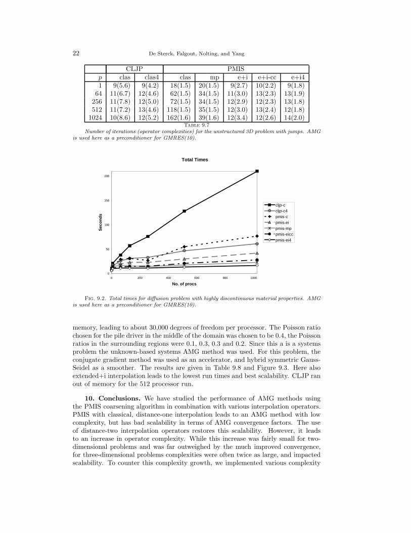
22 De Sterck, Falgout, Nolting, and Yang
CLJP PMISp clas clas4 clas mp e+i e+i-cc e+i41 9(5.6) 9(4.2) 18(1.5) 20(1.5) 9(2.7) 10(2.2) 9(1.8)
64 11(6.7) 12(4.6) 62(1.5) 34(1.5) 11(3.0) 13(2.3) 13(1.9)256 11(7.8) 12(5.0) 72(1.5) 34(1.5) 12(2.9) 12(2.3) 13(1.8)512 11(7.2) 13(4.6) 118(1.5) 35(1.5) 12(3.0) 13(2.4) 12(1.8)
1024 10(8.6) 12(5.2) 162(1.6) 39(1.6) 12(3.4) 12(2.6) 14(2.0)Table 9.7
Number of iterations (operator complexities) for the unstructured 3D problem with jumps. AMGis used here as a preconditioner for GMRES(10).
Total Times
0
50
100
150
200
0 200 400 600 800 1000
No. of procs
Sec
on
ds
cljp-ccljp-c4pmis-cpmis-eipmis-mppmis-eiccpmis-ei4
Fig. 9.2. Total times for diffusion problem with highly discontinuous material properties. AMGis used here as a preconditioner for GMRES(10).
memory, leading to about 30,000 degrees of freedom per processor. The Poisson ratiochosen for the pile driver in the middle of the domain was chosen to be 0.4, the Poissonratios in the surrounding regions were 0.1, 0.3, 0.3 and 0.2. Since this a is a systemsproblem the unknown-based systems AMG method was used. For this problem, theconjugate gradient method was used as an accelerator, and hybrid symmetric Gauss-Seidel as a smoother. The results are given in Table 9.8 and Figure 9.3. Here alsoextended+i interpolation leads to the lowest run times and best scalability. CLJP ranout of memory for the 512 processor run.
10. Conclusions. We have studied the performance of AMG methods usingthe PMIS coarsening algorithm in combination with various interpolation operators.PMIS with classical, distance-one interpolation leads to an AMG method with lowcomplexity, but has bad scalability in terms of AMG convergence factors. The useof distance-two interpolation operators restores this scalability. However, it leadsto an increase in operator complexity. While this increase was fairly small for two-dimensional problems and was far outweighed by the much improved convergence,for three-dimensional problems complexities were often twice as large, and impactedscalability. To counter this complexity growth, we implemented various complexity

Distance-two interpolation for parallel AMG 23
CLJP PMISp clas clas4 clas mp e+i e+i-cc e+i-ccs e+i41 64 63 94 93 68 69 72 728 83 84 159 131 89 95 96 90
64 92 96 210 179 97 105 112 107512 - 112 319 247 108 109 123 123Cop 4.5-7.3 3.6-5.4 1.5 1.5 2.5-3.0 2.1-2.4 1.9-2.1 1.9-2.0
Table 9.8
Number of iterations for the 3D elasticity problem; range of operator complexities. AMG isused here as a preconditioner for conjugate gradient.
0
50
100
150
200
250
300
350
400
0 100 200 300 400 500
no. of procs
tim
es in
sec
on
ds cljp-c
cljp-c4
pmis-c
pmis-mp
pmis-ei
pmis-eicc
pmis-eicc1
pmis-ei4
Fig. 9.3. Total times for the 3D elasticity problem. AMG is used here as a preconditioner forconjugate gradient.
reducing strategies, such as the use of smaller interpolatory sets and interpolationtruncation. The resulting AMG methods, particularly the extended and extended+iinterpolation in combination with truncation, lead to very good scalability for a vari-ety of difficult PDE problems on large parallel computers.
Acknowledgments. We thank Tzanio Kolev for providing the unstructured prob-lem generator and Jeff Painter for the Jacobi interpolation routine. This work wasperformed under the auspices of the U.S. Department of Energy by University of Cal-ifornia Lawrence Livermore National Laboratory under contract No. W-7405-Eng-48.
REFERENCES
[1] A. Baker, R. D. Falgout, U. M. Yang, An assumed partition algorithm for determining processorinter-communication, Parallel Computing 32 (2006), 394–414.
[2] A. Brandt, S. F. McCormick, and J. W. Ruge, Algebraic multigrid (AMG) for sparse matrixequations, in Sparsity and Its Applications, D. J. Evans, ed., Cambridge University Press,Cambridge, 1984.
[3] J. Butler, Improving coarsening and interpolation for algebraic multigrid, Master’s thesis inApplied Mathematics, University of Waterloo (2006).
24 De Sterck, Falgout, Nolting, and Yang
[4] W. L. Briggs, V. E. Henson, and S. F. McCormick, A Multigrid Tutorial (SIAM, Philadelphia,PA, second ed., 2000).
[5] A. J. Cleary, R. D. Falgout, V. E. Henson, and J. E. Jones, Coarse grid selection for parallel al-gebraic multigrid, in Proceedings of the fifth international symposium on solving irregularlystructured problems in parallel (Springer-Verlag, New York, 1998).
[6] A. J. Cleary, R. D. Falgout, V. E. Henson, J. E. Jones, T. A. Manteuffel, S. F. McCormick,G. N. Miranda, and J. W. Ruge, Robustness and scalability of algebraic multigrid, SIAMJournal on Scientific Computing, 21 (2000), 1886–1908.
[7] H. De Sterck, U. M. Yang, and J. J. Heys, Reducing Complexity in Parallel Algebraic MultigridPreconditioners, SIAM Journal on Matrix Analysis and Applications 27 (2006) 1019–1039.
[8] R. D. Falgout, J.E. Jones, and U.M. Yang, Pursuing scalability for hypre’s conceptual inter-faces, ACM Trans. Math. Softw. 31 (2005) 326–350.
[9] V. E. Henson and U. M. Yang, BoomerAMG: a parallel algebraic multigrid solver and precon-ditioner, Applied Numerical Mathematics 41 (2002) 155–177.
[10] M. Luby, A simple parallel algorithm for the maximal independent set problem, SIAM Journalon Computing 15 (1986) 1036–1053.
[11] J. W. Ruge and K. Stuben, Algebraic multigrid (AMG), in : S. F. McCormick, ed., MultigridMethods, vol. 3 of Frontiers in Applied Mathematics (SIAM, Philadelphia, 1987) 73–130.
[12] K. Stuben, Algebraic multigrid (AMG): an introduction with applications, in : U. Trottenberg,C. Oosterlee and A. Schuller, eds., Multigrid (Academic Press, 2000).


![New Iterative Methods for Interpolation, Numerical ... · and Aitken’s iterated interpolation formulas[11,12] are the most popular interpolation formulas for polynomial interpolation](https://static.fdocuments.in/doc/165x107/5ebfad147f604608c01bd287/new-iterative-methods-for-interpolation-numerical-and-aitkenas-iterated-interpolation.jpg)


![New INTERPOLATION OF EISENSTEIN-KRONECKER NUMBERS … · 2008. 2. 2. · arXiv:math/0610163v4 [math.NT] 11 Dec 2007 ALGEBRAIC THETA FUNCTIONS AND THE p-ADIC INTERPOLATION OF EISENSTEIN-KRONECKER](https://static.fdocuments.in/doc/165x107/6067a04aa3c18e5a0c0d62c6/new-interpolation-of-eisenstein-kronecker-numbers-2008-2-2-arxivmath0610163v4.jpg)