Distance-based accessibility indices∗

Laszlo Csato†

Department of Operations Research and Actuarial SciencesCorvinus University of Budapest

MTA-BCE ”Lendulet” Strategic Interactions Research GroupBudapest, Hungary

October 27, 2017

Abstract

The paper attempts to develop a suitable accessibility index for networks whereeach link has a value such that a smaller number is preferred like distance, cost, ortravel time. A measure called distance sum is characterized by three independentproperties: anonymity, an appropriately chosen independence axiom, and dominancepreservation, which requires that a node not far to any other is at least as accessible.

We argue for the need of eliminating the independence property in certainapplications. Therefore generalized distance sum, a family of accessibility indices,will be suggested. It is linear, considers the accessibility of vertices besides theirdistances and depends on a parameter in order to control its deviation from distancesum. Generalized distance sum is anonymous and satisfies dominance preservationif its parameter meets a sufficient condition. Two detailed examples demonstrate itsability to reflect the vulnerability of accessibility to link disruptions.

JEL classification number: D85, Z13

AMS classification number: 15A06, 91D30

Keywords: Network; geography; accessibility; distance sum; axiomatic approach

1 IntroductionSection 1 aims to confirm the importance of accessibility indices. Some applications of themare presented in Subsection 1.1 together with a detailed literature review in Subsection 1.2.Finally, Subsection 1.3 gives an outline of our approach and main results.∗ We are grateful to Dezso Bednay for useful advices.

The research was supported by OTKA grant K 111797 and MTA-SYLFF (The Ryoichi Sasakawa YoungLeaders Fellowship Fund) grant ’Mathematical analysis of centrality measures’, awarded to the author in2015.† e-mail: laszlo.csato@uni-corvinus.hu

1

arX

iv:1

507.

0146

5v3

[cs

.SI]

26

Oct

201

7

1.1 MotivationA key and basic concept in network analysis that researchers want to capture is centrality.The well-known classification of Freeman (1979) distinguishes three conceptions, measuredby degree, closeness, and betweenness, respectively. However, there is a frequent need forother centrality models. One of them, mainly used in theoretical geography for analysingsocial activities and regional economies, can be called accessibility. Accessibility indexprovides a numerical answer to questions such as ’How accessible is a node from othernodes in a network?’ or ’What is its relative geographical importance?’.

Accessibility measures have a number of interesting ways of utilization:

1. Knowledge of which nodes have the highest accessibility could be of interest in itself(e.g. by revealing their strategic importance);

2. The accessibility of vertices could be statistically correlated to other economic,sociological or political variables;

3. Accessibility of the same nodes (e.g. urban centres) in different (e.g. transportation,infrastructure) networks could be compared;

4. Proposed changes in a network could be evaluated in terms of their effect on theaccessibility of vertices;

5. Networks (e.g. empires) could be compared by their propensity to disintegrate. Forexample, it may be difficult to manage from a unique centre if the most accessiblenodes are far from each other.

Practical application of accessibility involve, among others, an analysis of the medievalriver trade network of Russia (Pitts, 1965, 1979), of the medieval Serbian oecumene(Carter, 1969), of the interstate highway network for cities in the southeastern UnitedStates (Garrison, 1960; Mackiewicz and Ratajczak, 1996), of the inter-island voyagingnetwork of the Marshall islands (Hage and Harary, 1995), or of the global maritimecontainer transportation network (Wang and Cullinane, 2008). Accessibility indices canbe used in operations research, too, where a typical problem is that of choosing a site fora facility on the basis of a specific criterion (Slater, 1981).

1.2 Some methods for measuring accessibilityThe adjacency matrix C of the network graph is given by cij = 1 if and only if nodes iand j are connected and cij = 0 otherwise.

One of the first accessibility indices, sometimes called connection array, was introducedby Garrison (1960). It is based on powering of matrix C such that

T = C + C2 + C3 + · · ·+ Cm =m∑i=1

Ci.

The accessibility of a node comes from summing the corresponding column of matrix T ,i.e. the total number of at most m-long paths to other nodes. It was used by Pitts (1965)and Carter (1969) despite two significant shortcomings:

• The increase of m distorts reality as some redundant paths (i.e. longer thanthe shortest path in a topological sense) are included in the calculation ofaccessibility.

2

• It is not obvious what is the appropriate value of m. The usual choice is thediameter, the maximum number of edges in the shortest path between thefurthest pair of nodes, which provides that T has only positive elements (ifm ≥ 2).

The first problem may be addressed by introducing a multiplier for Ci showing exponentialdecay in the calculation of matrix T , as suggested by Garrison (1960) following Katz(1953). However, it is still not able to completely overcome the inherent failures of themethod (Mackiewicz and Ratajczak, 1996).

In order to improve the comparability of results achieved for various m, Stutz (1973)proposed a formula to determine the relative accessibility of nodes.

Naturally, one can focus only on the shortest paths between the nodes. Then a plausiblemeasure is the total length of them to all other nodes (Shimbel, 1951, 1953; Harary, 1959;Pitts, 1965; Carter, 1969), which is called shortest-path array.

Betweenness measures how many shortest paths pass through the given node (Shimbel,1953; Freeman, 1977). It was also applied as an accessibility index (Pitts, 1979).

Eccentricity concentrates on the maximum distance to all other nodes. Sometimes it isthe suitable concept for predicting the politically and symbolically important nodes in anetwork (Hage and Harary, 1995).

A whole branch of literature, initiated by (Gould, 1967), propagates the use of eigen-vectors for measuring accessibility (Carter, 1969; Tinkler, 1972; Straffin, 1980; Mackiewiczand Ratajczak, 1996; Wang and Cullinane, 2008). It is based on the Perron-Frobeniustheorem (Perron, 1907; Frobenius, 1908, 1909, 1912) for nonnegative square matrices:matrix C has a unique (up to constant multiples) positive eigenvector corresponding tothe principal eigenvalue. It have been proposed that the non-principal eigenvectors mightalso have geographical meaning, however, its use remains controversial (Carter, 1969; Hay,1975; Tinkler, 1975; Straffin, 1980).

Finally, Amer et al. (2012) construct accessibility indices to the nodes of directedgraphs using methods of game theory.

1.3 Aims and toolsThe focus on the adjacency matrix has no sense in some applications, where the networkgraph is closely complete (Wang and Cullinane, 2008). However, as Taaffe and Gauthier(1973) claim, it is not necessary to restrict the concept to a purely topological one. Value oflinkages may be given as a distance between the nodes in actual mileage as well as the costof movement or the time required to travel between them. Actually, it was implementedby Carter (1969) and Pitts (1979) using the distance as a value.

We will call the edge values distance throughout the paper. It may be any measuresatisfying triangle inequality such that a smaller value is better. It can be assumed withoutloss of generality that the network is complete, i.e. a value is available for each link. Whilethe extension of shortest-path array to this domain, said to be the distance sum, is obvious,the applicability of other measures – presented in Subsection 1.2 – is ambiguous, despitethe use of the principal eigenvector by Wang and Cullinane (2008).

The paper aims to analyse accessibility indices in these networks. For this purposethe axiomatic approach, a standard path in game and social choice theory will be applied.Distance sum will be characterized, that is, a set of properties will be given such that it isthe only accessibility index satisfying them, but eliminating any axiom allows for othermeasures. According to our knowledge, no axiomatizations of accessibility indices exist.

3

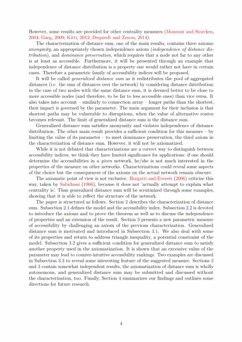
However, some results are provided for other centrality measures (Monsuur and Storcken,2004; Garg, 2009; Kitti, 2012; Dequiedt and Zenou, 2014).

The characterization of distance sum, one of the main results, contains three axioms:anonymity, an appropriately chosen independence axiom (independence of distance dis-tribution), and dominance preservation, which requires that a node not far to any otheris at least as accessible. Furthermore, it will be presented through an example thatindependence of distance distribution is a property one would rather not have in certaincases. Therefore a parametric family of accessibility indices will be proposed.

It will be called generalized distance sum as it redistributes the pool of aggregateddistances (i.e. the sum of distances over the network) by considering distance distribution:in the case of two nodes with the same distance sum, it is deemed better to be close tomore accessible nodes (and therefore, to be far to less accessible ones) than vice versa. Italso takes into account – similarly to connection array – longer paths than the shortest,their impact is governed by the parameter. The main argument for their inclusion is thatshortest paths may be vulnerable to disruptions, when the value of alternative routesbecomes relevant. The limit of generalized distance sum is the distance sum.

Generalized distance sum satisfies anonymity and violates independence of distancedistribution. The other main result provides a sufficient condition for this measure – bylimiting the value of its parameter – to meet dominance preservation, the third axiom inthe characterization of distance sum. However, it will not be axiomatized.

While it is not debated that characterizations are a correct way to distinguish betweenaccessibility indices, we think they have limited significance for applications: if one shoulddetermine the accessibilities in a given network, he/she is not much interested in theproperties of the measure on other networks. Characterizations could reveal some aspectsof the choice but the consequences of the axioms on the actual network remain obscure.

The axiomatic point of view is not exclusive. Borgatti and Everett (2006) criticize thisway, taken by Sabidussi (1966), because it does not ’actually attempt to explain whatcentrality is’. Thus generalized distance sum will be scrutinized through some examples,showing that it is able to reflect the structure of the network.

The paper is structured as follows. Section 2 describes the characterization of distancesum. Subsection 2.1 defines the model and the accessibility index. Subsection 2.2 is devotedto introduce the axioms and to prove the theorem as well as to discuss the independenceof properties and an extension of the result. Section 3 presents a new parametric measureof accessibility by challenging an axiom of the previous characterization. Generalizeddistance sum is motivated and introduced in Subsection 3.1. We also deal with someof its properties and return to address triangle inequality, a potential constraint of themodel. Subsection 3.2 gives a sufficient condition for generalized distance sum to satisfyanother property used in the axiomatization. It is shown that an excessive value of theparameter may lead to counter-intuitive accessibility rankings. Two examples are discussedin Subsection 3.3 to reveal some interesting feature of the suggested measure. Sections 2and 3 contain somewhat independent results, the axiomatization of distance sum is whollyautonomous, and generalized distance sum may be submitted and discussed withoutthe characterization, too. Finally, Section 4 summarizes our findings and outlines somedirections for future research.

4

2 A characterization of distance sumIn this section, some natural conditions will be conceived for accessibility indices, similarlyto centrality measures (Sabidussi, 1966; Chien et al., 2004; Landherr et al., 2010; Boldi andVigna, 2014). Distance sum, an obvious solution for our problem, will be characterized,that is, a set of properties will be given such that it is the only accessibility index satisfyingthem, while eliminating any axiom allows for other measures.

2.1 The modelDefinition 1. Transportation network: Transportation network is a pair (N,D) such that

• N = {1, 2, . . . , n} is a finite set of nodes;

• D ∈ Rn×n+ is a symmetric distance matrix satisfying triangle inequality, namely,

dij ≤∑m−1`=0 dk`k`+1 where (i = k0, k1, . . . , km = j) is a path between the nodes i

and j. dii = 0 for all i = 1, 2, . . . , n.

D can be the adjacency matrix of a complete, weighted, undirected graph (withoutloops and multiple edges) with the set of nodes N .1

Notation 1. N n is the class of all transportation networks (N,D) with |N | = n.

Definition 2. Accessibility index: Let (N,D) ∈ N n be a transportation network. Ac-cessibility index f is a function that assigns an n-dimensional vector of real numbers to(N,D) with fi(N,D) showing the accessibility of node i.

Notation 2. f : N n → Rn is an accessibility index.Node i is said to be at least as accessible as node j in the transportation network (N,D)

if and only if fi(N,D) ≤ fj(N,D), so a smaller value of accessibility is more favourable.

Definition 3. Order equivalence: Let f, g : N n → Rn be two accessibility indices. Theyare called order equivalent if and only if fi(N,D) ≤ fj(N,D)⇔ fi(N,D) ≤ fj(N,D) forany transportation network (N,D) ∈ N n. .

Notation 3. f ≈ g means that accessibility measures f, g : N n → Rn are order equivalent.Since we focus on accessibility rankings, order equivalent accessibility indices are not

distinguished. For example, an accessibility index is invariant under multiplication bypositive scalars.

Throughout the paper, vectors are denoted by bold fonts and assumed to be columnvectors. Let e ∈ Rn be the column vector such that ei = 1 for all i = 1, 2, . . . , n andI ∈ Rn×n be the matrix with Iij = 1 for all i, j = 1, 2, . . . , n.

The first, almost trivial idea to measure accessibility can be the sum of distances to allother nodes. In fact, it is extensively used in the literature (Shimbel, 1951, 1953; Harary,1959; Pitts, 1965; Carter, 1969).

Definition 4. Distance sum: dΣ : N n → Rn such that dΣi = ∑

j∈N dij for all i ∈ N .1 Assumption of completeness is not restrictive in the case of connected graphs since the distance of

any pair of nodes can be measured by the shortest path between them.

5

2.2 Axioms and characterizationThe first condition is independence of the labelling of the nodes.

Definition 5. Anonymity (ANO): Let (N,D), (σN, σD) ∈ N be two transportationnetworks such that (σN, σD) is given by a permutation of nodes σ : N → N from (N,D).Accessibility index f : N n → Rn is called anonymous if fi(N,D) = fσi(σN, σD) for alli ∈ N .

Property ANO implies that two symmetric nodes are equally accessible. It also ensuresthat all nodes have the same accessibility in a transportation network with the samedistance between any pair of nodes.

Lemma 1. Distance sum satisfies ANO.

While distance sum is usually a good baseline to approximate accessibility, it does notconsider the distribution of distances.

Definition 6. Independence of distance distribution (IDD): Let (N,D) ∈ N n be atransportation network and i, j, k, ` ∈ N be four distinct nodes. Let f : N n → Rn be anaccessibility index such that fi(N,D) ≤ fj(N,D) and (N,D′) ∈ N n be a transportationnetwork identical to (N,D) except for d′ik 6= dik and d′i` 6= di` but d′ik + d′i` = dik + di`.f is called independent of distance distribution if fi(N,D′) ≤ fj(N,D′).

Property IDD implies that the accessibility ranking does not change if the distancesum of each node remains the same.

Lemma 2. Distance sum satisfies IDD.

Definition 7. Dominance: Let (N,D) ∈ N n be a transportation network and i, j ∈ Nbe two distinct nodes such that dik ≤ djk for all k ∈ N \ {i, j} with a strict inequality (<)for at least one k.Then it is said that node i dominates node j.

A natural requirement for accessibility indices can be that the accessibility of ’obviously’more external nodes is worse.

Definition 8. Dominance preservation (DP ): Let (N,D) ∈ N n be a transportationnetwork and i, j ∈ N be two distinct nodes such that node i dominates node j.Accessibility index f : N n → Rn preserves dominance if fi(N,D) < fj(N,D).

Property DP demands that if node j is at least as far from all nodes as node i, thenit has a larger accessibility value provided that they could not be labelled arbitrarily. Asimilar axiom called self-consistency has been suggested by (Chebotarev and Shamis, 1997)for preference aggregating methods.

Lemma 3. Distance sum satisfies DP .

Requirements ANO, IDD and DP still give a characterization of distance sum.

Theorem 1. If an accessibility index f : N n → Rn is anonymous, independent of distancedistribution and preserves dominance, then f is the distance sum.

6

Proof. Consider a transportation network (N,D) ∈ N n and three nodes i, j, k ∈ N . It canbe assumed that ∑m∈N dim ≤

∑m∈N djm. Define the transportation network (N,D′) ∈ N n

such that d′im = dim for all m ∈ N , d′jk = d′ik+(∑m∈N djm −∑m∈N dim) ≤ d′ik and d′j` = d′i`

for all ` ∈ N \ {i, j, k}. Two cases can be distinguished:

• ∑m∈N dim <∑m∈N djm

Then d′ik < d′jk, so fi(N,D′) < fj(N,D′) due to DP and fi(N,D) < fj(N,D)because of IDD as ∑m∈N d

′im = ∑

m∈N dim and ∑m∈N d′jm = ∑

m∈N djm.

• ∑m∈N dim = ∑m∈N djm

Then d′ik = d′jk, so fi(N,D′) = fj(N,D′) due to ANO and fi(N,D) = fj(N,D)because of IDD as ∑m∈N d

′im = ∑

m∈N dim and ∑m∈N d′jm = ∑

m∈N djm.

It implies that f ≈ dΣ.

Remark 1. The proof of Theorem 1 requires at least three nodes. However, IDD has ameaning only for four nodes. It can be seen that ANO and DP are enough to characterizedistance sum if n = 3 since dik < djk ⇒ fi(N,D) < fj(N,D) because of dominancepreservation and dik = djk ⇒ fi(N,D) = fj(N,D) due to anonymity. Note that dij ≤dik ⇔

∑m∈N dim ≤

∑m∈N djm by definition.

Now the independence of the axioms is addressed.

Proposition 1. Anonymity, independence of distance distribution and domination preser-vation are logically independent conditions.

Proof. As usual, an example will be given that satisfies all the axioms mentioned inTheorem 1 except for the one under consideration. Consider the following three functions:Definition 9. Distance sum without ties: dΣ< : N n → Rn such that dΣ<

i = ∑j∈N dij +

(i− 1) min {∑`∈N (dj` − dk`) : j, k ∈ N} /n for all i ∈ N .Definition 10. Inverse distance sum: d−Σ : N n → Rn such that d−Σ

i = −∑j∈N dij forall i ∈ N .Definition 11. Distance product: dΠ : N n → Rn such that dΠ

i = ∏j 6=i dij for all i ∈ N .

Distance sum without ties satisfies IDD and DP but violates ANO as in the case ofequal distance sums, the node with a lower index becomes more accessible.

Inverse distance sum satisfies ANO and IDD but violates DP .Distance product satisfies ANO and DP but it is not equivalent to distance sum.

Figure 1: Transportation network of Example 1

1

2 3

4

3

6

3

1

3 5

7

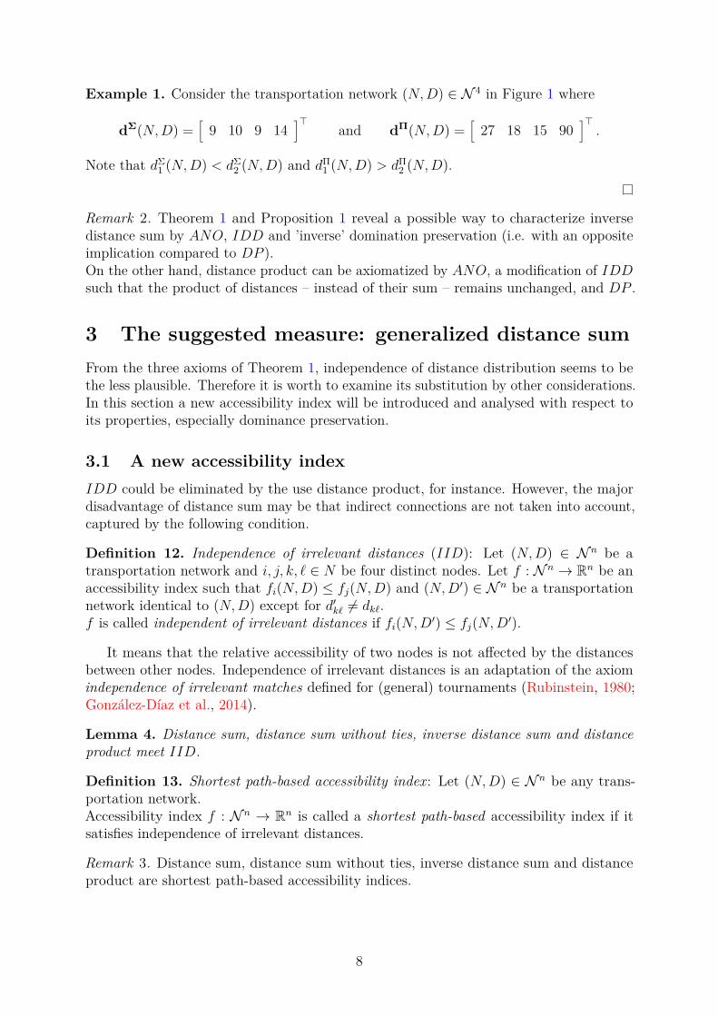
Example 1. Consider the transportation network (N,D) ∈ N 4 in Figure 1 where

dΣ(N,D) =[

9 10 9 14]>

and dΠ(N,D) =[

27 18 15 90]>.

Note that dΣ1 (N,D) < dΣ

2 (N,D) and dΠ1 (N,D) > dΠ

2 (N,D).

Remark 2. Theorem 1 and Proposition 1 reveal a possible way to characterize inversedistance sum by ANO, IDD and ’inverse’ domination preservation (i.e. with an oppositeimplication compared to DP ).On the other hand, distance product can be axiomatized by ANO, a modification of IDDsuch that the product of distances – instead of their sum – remains unchanged, and DP .

3 The suggested measure: generalized distance sumFrom the three axioms of Theorem 1, independence of distance distribution seems to bethe less plausible. Therefore it is worth to examine its substitution by other considerations.In this section a new accessibility index will be introduced and analysed with respect toits properties, especially dominance preservation.

3.1 A new accessibility indexIDD could be eliminated by the use distance product, for instance. However, the majordisadvantage of distance sum may be that indirect connections are not taken into account,captured by the following condition.

Definition 12. Independence of irrelevant distances (IID): Let (N,D) ∈ N n be atransportation network and i, j, k, ` ∈ N be four distinct nodes. Let f : N n → Rn be anaccessibility index such that fi(N,D) ≤ fj(N,D) and (N,D′) ∈ N n be a transportationnetwork identical to (N,D) except for d′k` 6= dk`.f is called independent of irrelevant distances if fi(N,D′) ≤ fj(N,D′).

It means that the relative accessibility of two nodes is not affected by the distancesbetween other nodes. Independence of irrelevant distances is an adaptation of the axiomindependence of irrelevant matches defined for (general) tournaments (Rubinstein, 1980;Gonzalez-Dıaz et al., 2014).

Lemma 4. Distance sum, distance sum without ties, inverse distance sum and distanceproduct meet IID.

Definition 13. Shortest path-based accessibility index: Let (N,D) ∈ N n be any trans-portation network.Accessibility index f : N n → Rn is called a shortest path-based accessibility index if itsatisfies independence of irrelevant distances.

Remark 3. Distance sum, distance sum without ties, inverse distance sum and distanceproduct are shortest path-based accessibility indices.

8

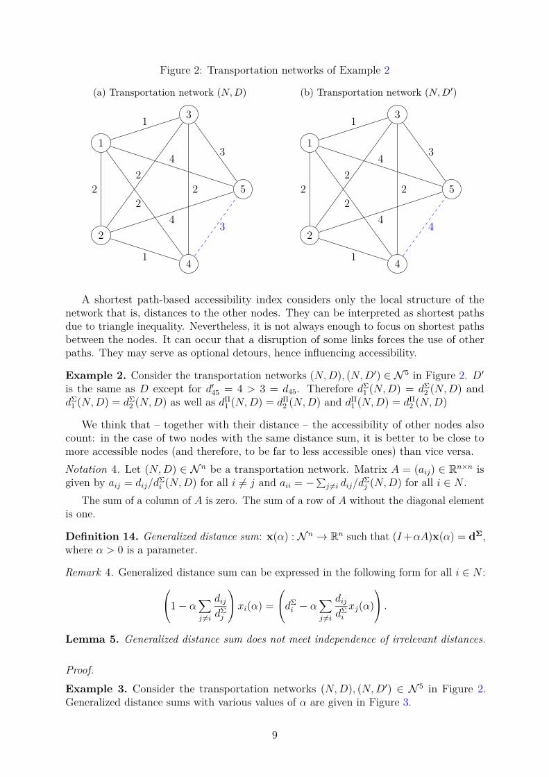
Figure 2: Transportation networks of Example 2

(a) Transportation network (N,D)

1

2

3

4

5

1

1

2

2

3

3

4

4

2 2

(b) Transportation network (N,D′)

1

2

3

4

5

1

1

2

2

3

4

4

4

2 2

A shortest path-based accessibility index considers only the local structure of thenetwork that is, distances to the other nodes. They can be interpreted as shortest pathsdue to triangle inequality. Nevertheless, it is not always enough to focus on shortest pathsbetween the nodes. It can occur that a disruption of some links forces the use of otherpaths. They may serve as optional detours, hence influencing accessibility.

Example 2. Consider the transportation networks (N,D), (N,D′) ∈ N 5 in Figure 2. D′is the same as D except for d′45 = 4 > 3 = d45. Therefore dΣ

1 (N,D) = dΣ2 (N,D) and

dΣ1 (N,D) = dΣ

2 (N,D) as well as dΠ1 (N,D) = dΠ

2 (N,D) and dΠ1 (N,D) = dΠ

2 (N,D)

We think that – together with their distance – the accessibility of other nodes alsocount: in the case of two nodes with the same distance sum, it is better to be close tomore accessible nodes (and therefore, to be far to less accessible ones) than vice versa.Notation 4. Let (N,D) ∈ N n be a transportation network. Matrix A = (aij) ∈ Rn×n isgiven by aij = dij/d

Σi (N,D) for all i 6= j and aii = −∑j 6=i dij/d

Σj (N,D) for all i ∈ N .

The sum of a column of A is zero. The sum of a row of A without the diagonal elementis one.

Definition 14. Generalized distance sum: x(α) : N n → Rn such that (I+αA)x(α) = dΣ,where α > 0 is a parameter.

Remark 4. Generalized distance sum can be expressed in the following form for all i ∈ N :1− α∑j 6=i

dijdΣj

xi(α) =dΣ

i − α∑j 6=i

dijdΣi

xj(α) .

Lemma 5. Generalized distance sum does not meet independence of irrelevant distances.

Proof.Example 3. Consider the transportation networks (N,D), (N,D′) ∈ N 5 in Figure 2.Generalized distance sums with various values of α are given in Figure 3.

9

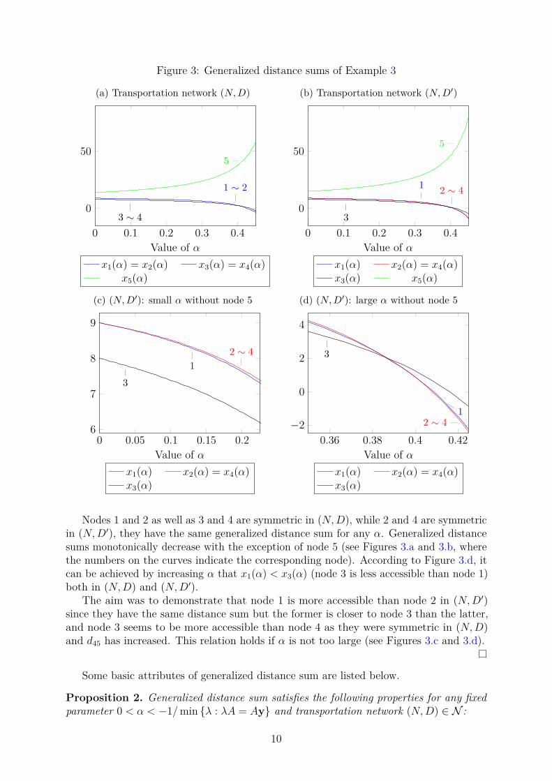
Figure 3: Generalized distance sums of Example 3

(a) Transportation network (N,D)

0 0.1 0.2 0.3 0.4

0

50

1 ∼ 2

3 ∼ 4

5

Value of αx1(α) = x2(α) x3(α) = x4(α)

x5(α)

(b) Transportation network (N,D′)

0 0.1 0.2 0.3 0.4

0

50

1 2 ∼ 4

3

5

Value of αx1(α) x2(α) = x4(α)x3(α) x5(α)

(c) (N,D′): small α without node 5

0 0.05 0.1 0.15 0.26

7

8

9

12 ∼ 4

3

Value of αx1(α) x2(α) = x4(α)x3(α)

(d) (N,D′): large α without node 5

0.36 0.38 0.4 0.42−2

0

2

4

12 ∼ 4

3

Value of αx1(α) x2(α) = x4(α)x3(α)

Nodes 1 and 2 as well as 3 and 4 are symmetric in (N,D), while 2 and 4 are symmetricin (N,D′), they have the same generalized distance sum for any α. Generalized distancesums monotonically decrease with the exception of node 5 (see Figures 3.a and 3.b, wherethe numbers on the curves indicate the corresponding node). According to Figure 3.d, itcan be achieved by increasing α that x1(α) < x3(α) (node 3 is less accessible than node 1)both in (N,D) and (N,D′).

The aim was to demonstrate that node 1 is more accessible than node 2 in (N,D′)since they have the same distance sum but the former is closer to node 3 than the latter,and node 3 seems to be more accessible than node 4 as they were symmetric in (N,D)and d45 has increased. This relation holds if α is not too large (see Figures 3.c and 3.d).

Some basic attributes of generalized distance sum are listed below.

Proposition 2. Generalized distance sum satisfies the following properties for any fixedparameter 0 < α < −1/min {λ : λA = Ay} and transportation network (N,D) ∈ N :

10

1. Existence and uniqueness: a unique vector of x(α) exists;

2. Anonymity (ANO);

3. Homogeneity (HOM): the relation

xi(α)(N,D) ≤ xi(α)(N,D)⇒ xi(α)(N, βD) ≤ xi(α)(N, βD)

holds for all i, j ∈ N and β > 0;

4. Distance sum conservation: ∑i∈N xi(α) = ∑i∈N d

Σi ;

5. Agreement: limα→0 x(α) = dΣ;

6. Flatness preservation (FP ): if dΣi = dΣ

j for all i, j ∈ N , then xi(α) = xj(α) for alli, j ∈ N .

Proof. We prove the statements above in the corresponding order.

1. Matrix (I + αA) is positive definite if 0 < α < −1/min {λ : λA = Ay}.

2. Generalized distance sum is invariant under isomorphism, it depends just on thestructure of the transportation network and not on the labelling of the nodes.

3. The identities dΣ(N, βD) = βdΣ(N,D) and A(N, βD) = A(N,D) implyx(α)(N, βD) = βx(α)(N,D).

4. ∑i∈N xi(α) = ∑i∈N

[xi(α) +∑

j∈N aijxj(α)]

= ∑i∈N d

Σi since ∑i∈N aij = 0 for all

j ∈ N .

5. limα→0 αAx(α) = 0.

6. xi(α) = dΣi satisfies (I + αA)x(α) = dΣ in the case of dΣ

i = dΣj for all i, j ∈ N .

Regarding ANO, it remains an interesting question whether the opposite of symmetryis valid, i.e., two nodes have the same generalized distance sum for any α > 0 only if theyare symmetric.

Homogeneity means that the accessibility ranking is invariant under the multiplicationof all distances by a positive scalar (i.e. the choice of measurement scale). Note thattriangle inequality is preserved when distances are multiplied by a positive scalar.

The name of this accessibility index comes from the property distance sum conservation:it can be interpreted as a way to redistribute the sum of distances among the nodes. Thisaxiom contributes to the comparability of calculated accessibilities across different networks.According to agreement, its limit is distance sum.

FP requires that generalized distance sum results in a tied accessibility between anynodes if distance sum also gives this result. The other direction (whether the flatness ofgeneralized distance for a given α implies the flatness of distance sum) requires furtherresearch.Remark 5. Distance sum also satisfies the properties listed in Proposition 2 (with theobvious exception of agreement). Distance product does not meet distance sum conservationand flatness preservation.

11

Figure 4: Transportation network of Example 4

1

2

3

4

5

10

9

8

7

6

Triangle inequality is essential for an accessibility index satisfying FP .

Example 4. Consider the transportation network (N,D) ∈ N 10 in Figure 4 such that

• dij = 1 if and only if nodes i and j are connected;

• dij = 10 if and only if nodes i and j are not connected.

Then dΣi = 3× 1 + 6× 10 = 63 for all i ∈ N , but nodes 5 and 6 seems to be more accessible

than the others. It is the case until dij > 2 in the case of not connected nodes i and jsince then there exists more shortcuts for nodes 5 and 6 than for the others.

It can be seen (e.g. from Example 3) that generalized distance sum is better able todistinguish the accessibility of nodes than distance sum. In other words, there are far lessnodes of equal generalized distance sum than there are for standard distance sum. It maybe important in some applications (Lindelauf et al., 2013).

3.2 Connection to domination preservationGeneralized distance sum was constructed in order to eliminate independence of distancedistribution. Proposition 2 shows that anonymity is preserved in the process. Now we turnto the third axiom in the characterization of distance sum by Theorem 1, and investigatewhether the suggested accessibility index meets domination preservation.Notation 5. mink{S} and maxk{S} are the kth smallest and largest element of a set S,respectively.

Theorem 2. Generalized distance sum satisfies DP if

α < min

min2{dΣi : i ∈ N

}max {xi(α) : i ∈ N} ;

min{dΣi : i ∈ N

}max {dΣ

i : i ∈ N}

.Proof. Consider a transportation network (N,D) ∈ N and two distinct nodes i, j ∈ Nsuch that dik ≤ djk for all k ∈ N \ {i, j} with a strict inequality (<) for at least one k.Then

xi(α) =1− α

∑k 6=i

dikdΣk

−1 ∑k 6=i

dik

(1− αxk(α)

dΣi

) and

12

xj(α) =1− α

∑k 6=j

djkdΣk

−1 ∑k 6=j

djk

(1− αxk(α)

dΣj

) .The following two conditions are sufficient for xi(α) < xj(α):

• αxk(α)/dΣj < 1 for any k ∈ N \ {i, j}, that is, α < dΣ

j /xk(α), which providesthat the ’contribution’ of djk to xj(α) is positive;

• α∑k 6=i dik/dΣk ≤ α

∑k 6=j djk/d

Σk ≤ αdΣ

j /min{dΣ` : ` ∈ N

}< 1, namely, α <

min{dΣ` : ` ∈ N

}/dΣ

j .

Note also that dΣj ≥ min2

{dΣ` : ` ∈ N

}.

Remark 6. According to the proof of Theorem 2, the condition

α < min{dΣi : i ∈ N

}/max {xi(α) : i ∈ N}

provides that the ’contribution’ of any distance to any node’s generalized distance sum ispositive, therefore it is positive, too (look at Figure 3.d).Remark 7. Due to the continuity of x(α), min2

{dΣi : i ∈ N

}> min

{dΣi : i ∈ N

}implies

min2{dΣi : i ∈ N

}max {xi(α) : i ∈ N} >

min{dΣi : i ∈ N

}max {dΣ

i : i ∈ N} ,

for small α, so the second expression is effective for small α. Nevertheless, usually the firstexpression limits the value of the parameter α.

In a certain sense, the result of Theorem 2 is not surprising because distance sum meetsDP and x(α) is ’close’ to it when α is small.2 The main contribution is the calculation ofa sufficient condition. It is not elegant since it depends on x(α), which excludes to checkthe requirement before the calculation,. However, ex post check is not difficult.Definition 15. Reasonable upper bound: Parameter α is reasonable if it satisfies thecondition of Theorem 2 for a transportation network (N,D) ∈ N . The largest α with thisproperty is the reasonable upper bound of the parameter.Notation 6. The reasonable upper bound of generalized distance sum’s parameter is α.Remark 8. Generalized degree satisfies DP for any reasonable α > 0.

It is analogous to the (dynamic) monotonicity of a preference aggregation methodcalled generalized row sum (Chebotarev, 1994, Property 13) as well as to the adding rankmonotonicity of a centrality measure generalized degree (Csato, 2015).

Violation of domination preservation may be a problem in practice.Example 5. Consider the transportation network (N,D′) ∈ N 5 in Figure 2, where node3 dominates node 1 since d3k ≤ d1k for k = 2, 4 and d35 < d15. However, x3(0.4) > x1(0.4)according to Figure 3.d.

Theorem 2 gives the reasonable upper bound as α ≈ 0.2686 from

α <min2

{dΣi : i ∈ N

}max {xi(α) : i ∈ N} .

Here min{dΣi : i ∈ N

}/max

{dΣi : i ∈ N

}= 8/15. However, Theorem 2 does not give a

necessary condition for DP since, for example, x3(0.36) < x1(0.36) in Figure 3.d.2 There always exists an appropriately small α satisfying the condition of Theorem 2.

13

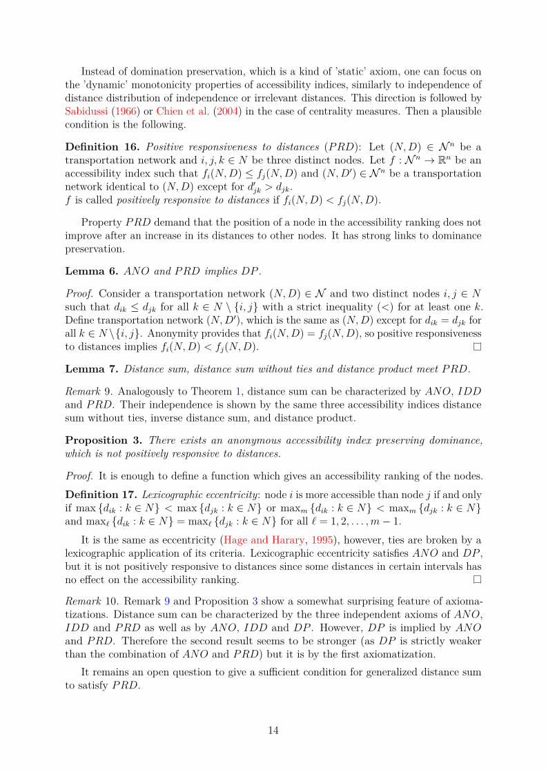
Instead of domination preservation, which is a kind of ’static’ axiom, one can focus onthe ’dynamic’ monotonicity properties of accessibility indices, similarly to independence ofdistance distribution of independence or irrelevant distances. This direction is followed bySabidussi (1966) or Chien et al. (2004) in the case of centrality measures. Then a plausiblecondition is the following.

Definition 16. Positive responsiveness to distances (PRD): Let (N,D) ∈ N n be atransportation network and i, j, k ∈ N be three distinct nodes. Let f : N n → Rn be anaccessibility index such that fi(N,D) ≤ fj(N,D) and (N,D′) ∈ N n be a transportationnetwork identical to (N,D) except for d′jk > djk.f is called positively responsive to distances if fi(N,D) < fj(N,D).

Property PRD demand that the position of a node in the accessibility ranking does notimprove after an increase in its distances to other nodes. It has strong links to dominancepreservation.

Lemma 6. ANO and PRD implies DP .

Proof. Consider a transportation network (N,D) ∈ N and two distinct nodes i, j ∈ Nsuch that dik ≤ djk for all k ∈ N \ {i, j} with a strict inequality (<) for at least one k.Define transportation network (N,D′), which is the same as (N,D) except for dik = djk forall k ∈ N \{i, j}. Anonymity provides that fi(N,D) = fj(N,D), so positive responsivenessto distances implies fi(N,D) < fj(N,D).

Lemma 7. Distance sum, distance sum without ties and distance product meet PRD.

Remark 9. Analogously to Theorem 1, distance sum can be characterized by ANO, IDDand PRD. Their independence is shown by the same three accessibility indices distancesum without ties, inverse distance sum, and distance product.

Proposition 3. There exists an anonymous accessibility index preserving dominance,which is not positively responsive to distances.

Proof. It is enough to define a function which gives an accessibility ranking of the nodes.Definition 17. Lexicographic eccentricity: node i is more accessible than node j if and onlyif max {dik : k ∈ N} < max {djk : k ∈ N} or maxm {dik : k ∈ N} < maxm {djk : k ∈ N}and max` {dik : k ∈ N} = max` {djk : k ∈ N} for all ` = 1, 2, . . . ,m− 1.

It is the same as eccentricity (Hage and Harary, 1995), however, ties are broken by alexicographic application of its criteria. Lexicographic eccentricity satisfies ANO and DP ,but it is not positively responsive to distances since some distances in certain intervals hasno effect on the accessibility ranking.

Remark 10. Remark 9 and Proposition 3 show a somewhat surprising feature of axioma-tizations. Distance sum can be characterized by the three independent axioms of ANO,IDD and PRD as well as by ANO, IDD and DP . However, DP is implied by ANOand PRD. Therefore the second result seems to be stronger (as DP is strictly weakerthan the combination of ANO and PRD) but it is by the first axiomatization.

It remains an open question to give a sufficient condition for generalized distance sumto satisfy PRD.

14

3.3 Two detailed examplesIn the previous discussion, generalized distance sum was only a ’tie-breaking rule’ ofdistance sum in the reasonable interval of the parameter α. Therefore, it remains to beseen whether the choice of a reasonable α may lead to significant changes in the accessibilityranking. The following examples reveal some interesting features of the measure, too.

Figure 5: Accessibility in the Ralik chain (see Example 6)

(a) The voyaging network graphof Marshall Islands’ Ralik chain

BikiniRongelap

Wotho

UjaeKwajalein

Lae

LibNamu

Ailinglaplap

Namorik Jaluit

Ebon

(b) Generalized distance sums

0 0.05 0.1 0.15 0.2 0.25 0.315

20

25

30

35

40

Bikini

Rongelap

Wotho

Ujae

LaeLib

Ailinglaplap

Jaluit

α

Value of αBikini Rongelap WothoUjae Lae Lib

Ailinglaplap Jaluit ∼ Namorik

Example 6. The Marshall Islands in eastern Micronesia are divided into two atoll chains,one of them is Ralik. Figure 5.a shows the graph of the voyaging network of this islandchain, constructed by Hage and Harary (1995). The distances of islands are measuredby the shortest path between them. For instance, the distance of Bikini and Jaluit is 5through Rongelap, Kwajalein, Namu and Ailinglaplap.

Note that Jaluit and Namorik are structurally equivalent in the network. Furthermore,Wotho dominates Rongelap and Ujae (it has extra links to Ujau and Lae, and to Bikiniand Rongelap, respectively); Wotho and Rongelap dominate Bikini; Lae dominates Ujae;Ailinglaplap, Namorik and Jaluit dominate Ebon.

Generalized distance sums are presented in Figure 5.b. The reasonable upper bound isα ≈ 0.2607, indicated by a (black) vertical line. However, the accessibility ranking doesnot violate DP for any α in Figure 5.b.

Kwajalein (with a distance sum of 20) and Namu (21) are the first and second nodesin the accessibility ranking for any α. The difference between their generalized distancesums monotonically increases. Ebon (34) is ’obviously’ the least accessible node for any α.These nodes do not appear in Figure 5.b.

Compared to the distance sum, the following changes can be observed in the reasonableinterval of α:

15

• The tie between Ailinglaplap and Wotho (25) is broken for Wotho. It makessense since the nodes around Wotho have more links among them.

• The tie between Rongelap and Ujae (27) is broken for Ujae. It is justified byUjae’s direct connection to Lae instead of Bikini as the former is more accessiblethan the latter.

• Lae (26) overtakes Ailinglaplap (25). The cause is that the network has essen-tially two components: the link between Ailinglaplap and Namu is a cut-edge,and the above part around Kwajalein (where Lae is located) is bigger and hasmore internal links.

Some other changes occur outside the reasonable interval of α: Rongelap and Ujau overtakeAilinglaplap as well as Bikini (34) overtakes Jaluit and Namorik (32). The reasoningapplied for the case of Ailinglaplap and Lae is relevant here, too, and it is difficult to argueagainst these modifications of the ranking.

Example 6 verifies that the analysis of accessibility rankings should not automaticallylimit to the reasonable interval of parameter α, sometimes it is worth to consider valuesoutside it. Remember that the condition of Theorem 2 is only sufficient, but not necessaryfor dominance preservation.

Example 7. Consider the network in Figure 6.a. The transportation network (N,D) ∈N 12 is such that the distances of nodes are measured by the shortest path between them.For example, d1,12 = 3 due to the path (1, 2)− (2, 11)− (11, 12).

Here node 1 dominates nodes 3, 8 and 9, node 2 dominates node 11, node 3 dominatesnode 9, node 5 dominates node 10 and node 11 dominates node 12.

Generalized distance sums are presented in Figure 6.b. The reasonable upper bound isα ≈ 0.279, indicated by a (black) vertical line. However, the accessibility ranking does notviolate DP for any α in Figure 6.b.

Node 1 (dΣ1 = 17) is ’obviously’ the most accessible node for any α. Nodes 11 (dΣ

11 = 29)and 12 (dΣ

12 = 37) are the last in the accessibility ranking for any reasonable value of α.The difference between their generalized distance sums monotonically increases. Thesenodes do not appear in Figure 6.b.

Note that x10(α) is not monotonic, it has a maximum around α = 0.145.Compared to the distance sum, the following changes can be observed in the reasonable

interval of α:

• The tie between nodes 3, 4, 5 and 7 (dΣ = 22) is broken in this order. Node3 is more accessible than node 5 since node 9 is more accessible than node 10.Node 3 is more accessible than node 7 since node 4 is more accessible than node8 (and it has an extra link to node 9). Node 4 is more accessible than node 5since node 3 is more accessible than node 6. Node 4 is more accessible thannode 7 as its neighbours are more accessible. Node 5 is more accessible thannode 7 since node 4 is more accessible than node 8 (and it has an extra link tonode 10). The tie breaks are highlighted in Figure 6.c.

• The relation of nodes 3 and 4 (dΣ = 22) is uncertain: both are connected tonode 1, while node 5 is more accessible than node 6 (favouring node 4) andnode 9 is more accessible than node 10 (favouring node 3). Node 3 benefitsfrom a small α as shown in Figure 6.d. However, one can see the negligible

16

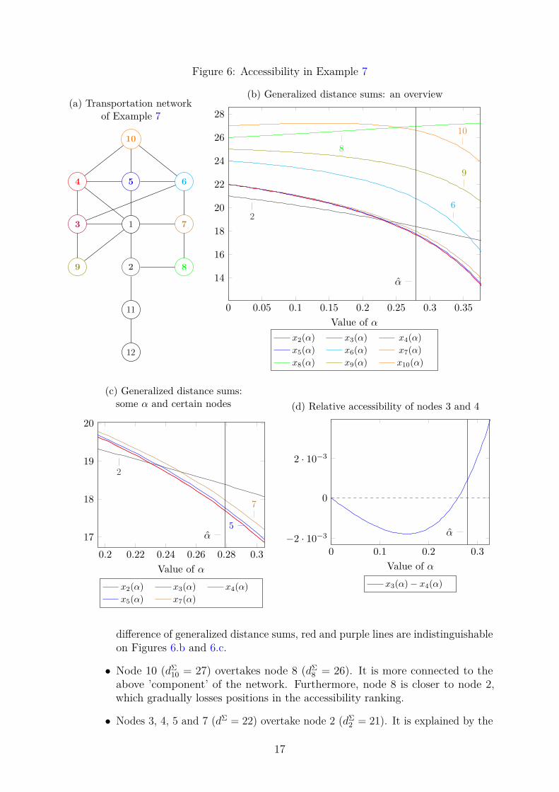
Figure 6: Accessibility in Example 7

(a) Transportation networkof Example 7

1

8

3

10

12

6

11

4 5

9 2

7

(b) Generalized distance sums: an overview

0 0.05 0.1 0.15 0.2 0.25 0.3 0.35

14

16

18

20

22

24

26

28

26

8

9

10

α

Value of αx2(α) x3(α) x4(α)x5(α) x6(α) x7(α)x8(α) x9(α) x10(α)

(c) Generalized distance sums:some α and certain nodes

0.2 0.22 0.24 0.26 0.28 0.317

18

19

20

2

5

7

α

Value of αx2(α) x3(α) x4(α)x5(α) x7(α)

(d) Relative accessibility of nodes 3 and 4

0 0.1 0.2 0.3−2 · 10−3

0

2 · 10−3

α

Value of αx3(α)− x4(α)

difference of generalized distance sums, red and purple lines are indistinguishableon Figures 6.b and 6.c.

• Node 10 (dΣ10 = 27) overtakes node 8 (dΣ

8 = 26). It is more connected to theabove ’component’ of the network. Furthermore, node 8 is closer to node 2,which gradually losses positions in the accessibility ranking.

• Nodes 3, 4, 5 and 7 (dΣ = 22) overtake node 2 (dΣ2 = 21). It is explained by the

17

latter’s vulnerable connections: if the link to node 1 is eliminated, then node 2suffers severe deterioration in its accessibility.

For larger α, node 6 (and even nodes 9 and 10) become(s) more accessible than node 2,too.

Example 7 illustrates that generalized distance sum may grab the vulnerability of somenodes’ accessibility to link disruptions. It can also reveal – analogously to the non-principaleigenvectors of the adjacency matrix – geographical subsystems of the network.

It is essential that any changes of the accessibility ranking in Examples 6 and 7 maybe attributable to the structure of the network graph.

4 Concluding remarksMeasuring accessibility is an important issue in network analysis. This paper has aimedto explore the methodological background of some accessibility indices for networksrepresented by a complete graph, where each link has a value such that a smaller numberis preferred (e.g. distance, cost, or travel time) and triangle inequality holds.

The obvious solution of distance sum is characterized by three independent axioms,anonymity, independence of distance distributions and dominance preservation. General-ized distance sum, a parametric family of linear accessibility indices, is suggested in orderto eliminate independence of distance distribution, a condition one would rather not havein certain applications. It considers the accessibility of vertices besides their distances (andgives an infinite depth to this argument) and depends on a parameter in order to controlits deviation from distance sum. Generalized distance sum seems to be promising withrespect to its properties, has a good level of differentiation, and gives acceptable resultson several transportation networks by making accessibility responsive to link disruptions.

Generalized distance sum – similarly to connection array – may get criticism fordepending on a seemingly arbitrary value. While it certainly causes some difficultiesin applications, parametrization is necessary to ensure the flexibility of the method.Alternative rankings should be regarded as revealing the uncertainty of accessibility. Aresearch pursuing normative goals could not assume the complex task of making decisions,

Although the suggested accessibility index offers a new way in the analysis of trans-portation networks, some issues have remained unanswered. The choice of parameterrequires further investigation and the characterization of generalized distance sum is wortha try. The behaviour of this index should be tested on other networks. Generalizeddistance sum may provide a basis for measuring the total accessibility of the network bya single number. Possible domain extensions include networks where the importance ofnodes is different, or the distance matrix is not symmetric. They will be considered forfuture research.

ReferencesAmer, R., Gimenez, J. M., and Magana, A. (2012). Accessibility measures to nodes of

directed graphs using solutions for generalized cooperative games. Mathematical Methodsof Operations Research, 75(1):105–134.

Boldi, P. and Vigna, S. (2014). Axioms for centrality. Internet Mathematics, 10(3-4):222–262.

18

Borgatti, S. P. and Everett, M. G. (2006). A graph-theoretic perspective on centrality.Social Networks, 28(4):466–484.

Carter, F. W. (1969). An analysis of the medieval Serbian oecumene: a theoreticalapproach. Geografiska Annaler. Series B, Human Geography, 51(1):39–56.

Chebotarev, P. (1994). Aggregation of preferences by the generalized row sum method.Mathematical Social Sciences, 27(3):293–320.

Chebotarev, P. and Shamis, E. (1997). A matrix-forest theorem and measuring relationsin small social groups (in Russian). Avtomatika i Telemekhanika, 58(9):125–137.

Chien, S., Dwork, C., Kumar, R., Simon, D. R., and Sivakumar, D. (2004). Link evolution:analysis and algorithms. Internet Mathematics, 1(3):277–304.

Csato, L. (2015). Measuring centrality by a generalization of degree. Corvinus EconomicsWorking Papers 2/2015, Corvinus University of Budapest, Budapest.

Dequiedt, V. and Zenou, Y. (2014). Local and consistent centrality measures in networks.Manuscript. https://www.gate.cnrs.fr/IMG/pdf/Dequiedt2015.pdf.

Freeman, L. C. (1977). A set of measures of centrality based on betweenness. Sociometry,40(1):35–41.

Freeman, L. C. (1979). Centrality in social networks: conceptual clarification. SocialNetworks, 1(3):215–239.

Frobenius, G. (1908). Uber Matrizen aus positiven Elementen I. Sitz.-Ber. Preuss. Akad.Wiss., Berlin:471–476.

Frobenius, G. (1909). Uber Matrizen aus positiven Elementen II. Sitz.-Ber. Preuss. Akad.Wiss., Berlin:514–518.

Frobenius, G. (1912). Uber Matrizen aus nicht negativen Elementen. Sitz.-Ber. Preuss.Akad. Wiss., Berlin:456–477.

Garg, M. (2009). Axiomatic foundations of centrality in networks. Manuscript. http://papers.ssrn.com/sol3/papers.cfm?abstract_id=1372441.

Garrison, W. L. (1960). Connectivity of the interstate highway system. Papers in RegionalScience, 6(1):121–137.

Gonzalez-Dıaz, J., Hendrickx, R., and Lohmann, E. (2014). Paired comparisons analysis:an axiomatic approach to ranking methods. Social Choice and Welfare, 42(1):139–169.

Gould, P. R. (1967). On the geographical interpretation of eigenvalues. Transactions ofthe Institute of British Geographers, (42):53–86.

Hage, P. and Harary, F. (1995). Eccentricity and centrality in networks. Social Networks,17(1):57–63.

Harary, F. (1959). Status and contrastatus. Sociometry, 22(1):23–43.

Hay, A. (1975). On the choice of methods in the factor analysis of connectivity matrices:a comment. Transactions of the Institute of British Geographers, (66):163–167.

19

Katz, L. (1953). A new status index derived from sociometric analysis. Psychometrika,18(1):39–43.

Kitti, M. (2012). Axioms for centrality scoring with principal eigenvectors. Manuscript.http://www.ace-economics.fi/kuvat/dp79.pdf.

Landherr, A., Friedl, B., and Heidemann, J. (2010). A critical review of centrality measuresin social networks. Business & Information Systems Engineering, 2(6):371–385.

Lindelauf, R. H. A., Hamers, H. J. M., and Husslage, B. G. M. (2013). Cooperative gametheoretic centrality analysis of terrorist networks: the cases of Jemaah Islamiyah and AlQaeda. European Journal of Operational Research, 229(1):230–238.

Mackiewicz, A. and Ratajczak, W. (1996). Towards a new definition of topologicalaccessibility. Transportation Research Part B: Methodological, 30(1):47–79.

Monsuur, H. and Storcken, T. (2004). Centers in connected undirected graphs: anaxiomatic approach. Operations Research, 52(1):54–64.

Perron, O. (1907). Zur Theorie der Matrices. Mathematische Annalen, 64(2):248–263.

Pitts, F. R. (1965). A graph theoretic approach to historical geography. The ProfessionalGeographer, 17(5):15–20.

Pitts, F. R. (1979). The medieval river trade network of Russia revisited. Social Networks,1(3):285–292.

Rubinstein, A. (1980). Ranking the participants in a tournament. SIAM Journal onApplied Mathematics, 38(1):108–111.

Sabidussi, G. (1966). The centrality index of a graph. Psychometrika, 31(4):581–603.

Shimbel, A. (1951). Applications of matrix algebra to communication nets. The Bulletinof Mathematical Biophysics, 13(3):165–178.

Shimbel, A. (1953). Structural parameters of communication networks. The Bulletin ofMathematical Biophysics, 15(4):501–507.

Slater, P. J. (1981). On locating a facility to service areas within a network. OperationsResearch, 29(3):523–531.

Straffin, P. D. (1980). Linear algebra in geography: eigenvectors of networks. MathematicsMagazine, 53(5):269–276.

Stutz, F. P. (1973). Accessibility and the effect of scalar variation on the poweredtransportation connection matrix. Geographical Analysis, 5(1):61–66.

Taaffe, E. J. and Gauthier, H. L. (1973). Geography of Transportation. Prentice-Hall, NewYersey.

Tinkler, K. J. (1972). The physical interpretation of eigenfunctions of dichotomous matrices.Transactions of the Institute of British Geographers, (55):17–46.

Tinkler, K. J. (1975). On the choice of methods in the factor analysis of connectivitymatrices: a reply. Transactions of the Institute of British Geographers, (66):168–171.

20

Wang, Y. and Cullinane, K. (2008). Measuring container port accessibility: an applicationof the principal eigenvector method (PEM). Maritime Economics & Logistics, 10(1):75–89.

21