Pricing Options through the Trinomial Tree

Ciaran Cox

Mathematical Sciences,

School of Information Systems, Computing and Mathematics,

Brunel University

Supervisor: Jacques-Elie Furter

2014

December 15, 2014

Abstract

I begin by a basic definition of option contracts and the pricing of these options through the

Black-Scholes model, which is based upon the Geometric Brownian Motion (GBM). Using this

model, one can solve for the implied volatility on an option through Newton’s iteration for find-

ing a root of a function. Binomial and trinomial lattice methods are alternate ways of pricing

options, but still assume that the stock price follows the GBM and constant volatility throughout

the option. European, American, Barrier and double barrier knockout options are priced using

the trinomial tree. Delta, Theta and Gamma Greeks are calculated through the Black-Scholes

model, with a comparison of prices on the Delta and Gamma through the trinomial tree. Using

these greeks, I move on to the delta-hedge rule and a delta tolerance applied practically to mar-

ket data from the Bloomberg terminals, with comparison of different strike prices on different

companies, concluding with a brief overview in to transaction costs.

Acknowledgements

A special thanks to my supervisor Jacques-Elie Furter for his increased support throughout my

project. Also like to thank my mum, dad and my sister for inspirational motivation throughout

my university studies, along with all my friends and a special thanks to Joel Johnson for excellent

support during the project.

Contents

1 Introduction 61.1 Geometric Brownian Motion (GBM) . . . . . . . . . . . . . . . . . . . . . . . 7

1.2 Black-Scholes Model . . . . . . . . . . . . . . . . . . . . . . . . . . . . . . . 8

1.2.1 Implied Volatility by the Black-Scholes Equation . . . . . . . . . . . . 10

2 Lattice models 112.1 Formulation of the Binomial Option Pricing Model by replicating portfolios . . 14

2.2 Binomial model to the Trinomial model . . . . . . . . . . . . . . . . . . . . . 15

3 Trinomial Tree 173.1 Pricing a European option through the Trinomial Tree . . . . . . . . . . . . . . 17

3.2 Pricing an American option through the Trinomial Tree . . . . . . . . . . . . . 19

3.3 Pricing a Barrier option through the Trinomial Tree . . . . . . . . . . . . . . . 20

3.4 Pricing a Double Barrier Knockout option through the Trinomial Tree . . . . . 23

4 The Greeks 254.1 Greeks via the Black-Scholes Model . . . . . . . . . . . . . . . . . . . . . . . 26

4.2 Delta and Gamma through the Trinomial Tree . . . . . . . . . . . . . . . . . . 29

5 Hedging Strategies 305.1 Delta-hedging rule . . . . . . . . . . . . . . . . . . . . . . . . . . . . . . . . 31

5.1.1 Delta-hedge rule across different companies . . . . . . . . . . . . . . . 32

5.2 Rebalancing under delta tolerance . . . . . . . . . . . . . . . . . . . . . . . . 34

5.3 Delta-hedging including Transaction Costs . . . . . . . . . . . . . . . . . . . . 35

6 Conclusion 36

1

7 Recommendations and Further Work 377.1 Implied Trinomial Tree . . . . . . . . . . . . . . . . . . . . . . . . . . . . . . 37

7.2 Further Hedging Techniques . . . . . . . . . . . . . . . . . . . . . . . . . . . 38

A my impvol.m Matlab file 39

B t treesize.m Matlab file 40

C tree barrier upcall.m Matlab file 41

D t double bar.m Matlab file 43

E g com.m Matlab file 44

F delta rebalance.m Matlab file 45

G delta rebalance tol.m Matlab file 47

H Background and Project Plan 49

Bibliography 57

Bibliography 59

2

List of Tables

3.1 Indicator Variables for Barrier Options . . . . . . . . . . . . . . . . . . . . . . 20

3.2 Indicator Variables Double Barrier Knockout Option . . . . . . . . . . . . . . 23

5.1 Delta-hedging rule comparison of companies . . . . . . . . . . . . . . . . . . 32

3

List of Figures

2.1 Non-Recombining Binomial Tree and a Recombining Binomial Tree . . . . . . 12

2.2 Multi Step Binomial Tree . . . . . . . . . . . . . . . . . . . . . . . . . . . . . 13

2.3 Binomial to Trinomial Formulation . . . . . . . . . . . . . . . . . . . . . . . . 15

2.4 Implied Google Call Option prices through the trinomial tree compared with

market prices . . . . . . . . . . . . . . . . . . . . . . . . . . . . . . . . . . . 16

3.1 European Call and Put Option Prices against Share price . . . . . . . . . . . . 18

3.2 Barrier Option Prices with varying barrier value . . . . . . . . . . . . . . . . . 21

3.3 Double Barrier Knockout Option . . . . . . . . . . . . . . . . . . . . . . . . . 24

4.1 Delta, Theta and Gamma Greeks via the Black-Scholes model varying time till

maturity . . . . . . . . . . . . . . . . . . . . . . . . . . . . . . . . . . . . . . 27

4.2 Delta, Theta and Gamma Greeks via the Black-Scholes model varying Strike Price 27

4.3 Delta, Theta and Gamma Greeks via the Black-Scholes model up to maturity . 28

4.4 Delta and Gamma Greeks via the Trinomial tree and the Black-Scholes model . 29

5.1 Delta-hedge rule, rebalancing every day . . . . . . . . . . . . . . . . . . . . . 32

5.2 Delta-hedging rule while varying Delta tolerance . . . . . . . . . . . . . . . . 34

7.1 Trinomial tree and an Implied trinomial tree ([22]) . . . . . . . . . . . . . . . 37

A.1 my impvol.m . . . . . . . . . . . . . . . . . . . . . . . . . . . . . . . . . . . 39

B.1 t treesize.m . . . . . . . . . . . . . . . . . . . . . . . . . . . . . . . . . . . . 40

C.1 tree barrier upcall.m (part a) . . . . . . . . . . . . . . . . . . . . . . . . . . . 41

C.2 tree barrier upcall.m (part b) . . . . . . . . . . . . . . . . . . . . . . . . . . . 42

D.1 t double bar.m, leaf vector discounted back through trinomial tree . . . . . . . 43

4

E.1 g com.m . . . . . . . . . . . . . . . . . . . . . . . . . . . . . . . . . . . . . . 44

F.1 delta rebalance.m (part a) . . . . . . . . . . . . . . . . . . . . . . . . . . . . . 45

F.2 delta rebalance.m (part b) . . . . . . . . . . . . . . . . . . . . . . . . . . . . . 46

G.1 delta rebalance tol.m (part a) . . . . . . . . . . . . . . . . . . . . . . . . . . . 47

G.2 delta rebalance tol.m (part b) . . . . . . . . . . . . . . . . . . . . . . . . . . . 48

H.1 Non-Recombining Binomial Tree(Left) and a Recombining Binomial Tree(Right) 52

H.2 Multi-Step Binomial Tree . . . . . . . . . . . . . . . . . . . . . . . . . . . . . 53

H.3 Trinomial Tree Example . . . . . . . . . . . . . . . . . . . . . . . . . . . . . 55

H.4 Volatility Smile . . . . . . . . . . . . . . . . . . . . . . . . . . . . . . . . . . 56

5

Chapter 1

Introduction

An option is a type of contract that gives the holder the right to, but not obligation to buy (call),

or sell (put) an underlying asset or instrument at a specified strike price on or before a specified

date. A European option can only be exercised at the maturity date while an American option

can be exercised at any point up to and including maturity. Pricing of these options, has been

around for a while, but in 1973 Fisher Black and Myron Scholes published a paper, ’The Pricing

of Options and Corporate Liabilities’([4]). They had an idea to hedge the option by buying or

selling the underlying asset in such a way to eliminate risk. With this they derived a stochastic

partial differential equation which estimates the price of the option over time. The Black-Scholes

equation led to a boom in finance and more specifically option trading around the world ([8]).

6

1.1 Geometric Brownian Motion (GBM)

A Geometric Brownian Motion is a continuous-time stochastic process where the logarithm of

the randomly varying quantity, follows a Wiener process with drift ([9]). A stochastic process St

is said to follow the GBM, if the process satisfies the following stochastic differential equation

(SDE);

dSt = µStdt +σStdWt , (1.1)

where,

• Wt is a Wiener process,

• σ is the percentage volatility,

• µ is the percentage drift,

solving equation (1.1) under Ito’s interpretation leads to ([10]),

St = S0e(µ−σ22 )t+σWt . (1.2)

The GBM assumes constant volatility when realistically in practice the volatility changes over

time, maybe stochastic ([13]). Further Extensions of the GBM are ”Stochastic Volatility models

in which the variance of a stochastic process is itself randomly distributed ([12]).” Below are

some stochastic volatility models ([13]);

• Heston Model.

• Constant Elasticity of Variance Model, CEV Model.

• Stochastic Alpha, Beta, Rho, (SABR Volatility model)

7

1.2 Black-Scholes Model

This model was first published by Fisher Black and Myron Scholes in their paper ”The Pricing

of Options and Corporate Liabilities”. (1973,[4]). Pricing of European options is based upon

there should not be any opportunities for risk-free profit in the market, (no-arbitrage principle).

Black and Scholes showed that ”it is possible to create a hedged position, consisting of a long

position in the stock and a short position in the option, whose value will not depend on the price

of the stock” ([4]). The Black-Scholes model is based upon the following assumptions;

• the stock price follows a Geometric Browian Motion,

• buying and selling any amount of stock with no transaction costs incurred,

• borrowing and lending takes place at the risk-free interest rate,

• non-dividend paying stock.

Under these assumptions the dynamic hedging strategy by Black and Scholes leads to the fol-

lowing partial differential equation;

∂V∂ t

+12

σ2S2 ∂ 2V

∂S2 + rs∂V∂S− rV = 0. (1.3)

This equation is solved with boundary conditions depending on the characteristics of the options.

For the standard European vanilla options we find explicit solutions leading to the Black-Scholes

formulas. The values of the European vanilla call and put options, respectively, are:

C(S, t) = N(d1)S−N(d2)Ke−r(T−t), (1.4)

P(S, t) = Ke−r(T−t)−S+C(S, t),

= N(−d2)Ke−r(T−t)−N(−d1)S, (1.5)

where

d1 =1

σ√

T − t[ln(

SK)+(r+

σ2

2)(T − t)], (1.6)

d2 =1

σ√

T − t[ln(

SK)+(r− σ2

2)(T − t)],

= d1−σ√

T − t. (1.7)

The quantities appearing in (1.4-1.7) are

8

• T − t being the time left till maturity,

• S is the stock price,

• K is the strike price,

• r is the risk-free rate,

• σ is the volatility of the underlying stock,

• N(·) being the cumulative normal distribution.

9

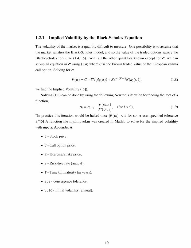
1.2.1 Implied Volatility by the Black-Scholes Equation

The volatility of the market is a quantity difficult to measure. One possibility is to assume that

the market satisfies the Black-Scholes model, and so the value of the traded options satisfy the

Black-Scholes formulae (1.4,1.5). With all the other quantities known except for σ , we can

set-up an equation in σ using (1.4) where C is the known traded value of the European vanilla

call option. Solving for σ

F(σ) =C−SN(d1(σ))+Ke−r(T−t)N(d2(σ)), (1.8)

we find the Implied Volatility ([5]).

Solving (1.8) can be done by using the following Newton’s iteration for finding the root of a

function,

σi = σi−1−F(σi−1)

F ′(σi−1), (for i > 0), (1.9)

”In practice this iteration would be halted once |F(σi)| < ε for some user-specified tolerance

ε .”[5] A function file my impvol.m was created in Matlab to solve for the implied volatility

with inputs, Appendix A;

• S - Stock price,

• C - Call option price,

• E - Exercise/Strike price,

• r - Risk-free rate (annual),

• T - Time till maturity (in years),

• eps - convergence tolerance,

• vol0 - Initial volatility (annual).

10

Chapter 2

Lattice models

Another method for pricing a stock option is, a lattice model. Which divides time from now up

to expiration into N discrete time points with each point going to two possible states (Binomial)

or three possible states (Trinomial) all the way up to expiration date where the expected payoffs

are calculated. Taking these payoffs and iteratively discounting the values back to the present by

the continuously discounted risk-free interest rate, applying risk-neutral probabilities through a

series of one-step trinomial trees until back with one node being the option price.

The first lattice model was the Binomial Option Pricing Model (BOPM) By Cox, Ross and

Rubinstein (CRR)(1979,[1]). From the source node the underlying asset either goes up with

probability p or down with probability 1− p. This process repeats until you reach the expiration

date with all the possible stock outcomes. The expected payoffs are then calculated at expiration

by:

Call Option = max{ST −K,0},

Put Option = max{K−ST ,0}.

ST being the stock price at expiration (T ) with K being the strike price on the option. Expected

payoffs are then discounted back through the tree by risk-neutral probabilities until you are back

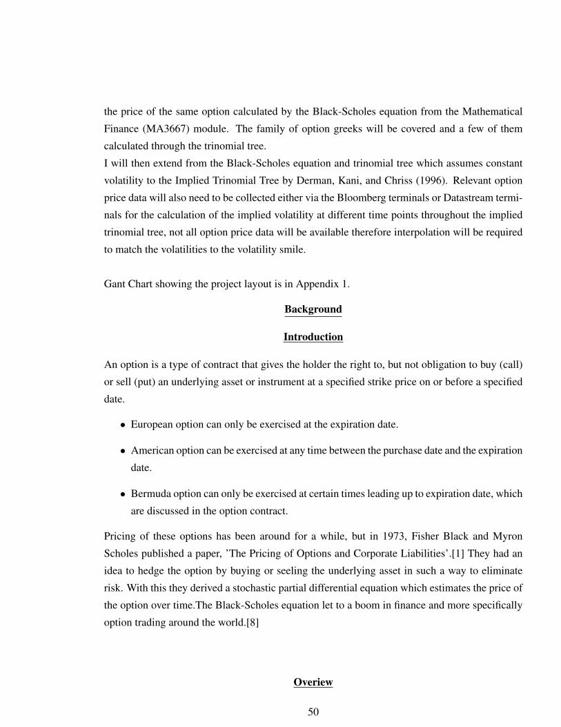
at the source node and reach the option price. Figure 2.1 below shows the Binomial Tree.

It is computationally efficient to have a recombining tree over a non-recombining tree, because

if the tree recombines, there are only N +1 nodes at stage N, whereas there will be 2N nodes at

stage N on a non-recombining tree. To make the tree recombine CRR ([1]) made ud = 1. There

are three parameters in Binomial model u,d, and p, we therefore need three equations to solve

uniquely for the parameters. First equation comes from matching the expectation of return on

11

Figure 2.1: Non-Recombining Binomial Tree and a Recombining Binomial Tree

http://www.mathworks.co.uk/help/fininst/overview-of-interest-rate-tree-models.html

the asset in a risk-neutral world. The second from matching the variance. We get

pu+(1− p)d = er∆t ,

pu2 +(1− p)d2− (er∆t)2

= σ2∆t.

The third equation comes from making the tree recombine ([1]),

u =1d.

After some rearranging and solving for the three parameters in the three equations above, results

showed[3]:

p =er∆t−du−d

,

u = eσ√

∆t ,

d = e−σ√

∆t ,

where σ is the assets volatility and r being the risk-free interest rate. When the Binomial tree

has been created shown in Figure 2.2[17] with the expected future payoffs (leaf nodes), these

need to be continuously discounted back to earlier nodes by the risk-free interest rate, taking

into account the risk-neutral probabilities.

The formula for calculating each node,

Cn, j = e−r∆t(pCn+1, j+1 +(1− p)Cn+1, j−1).

12

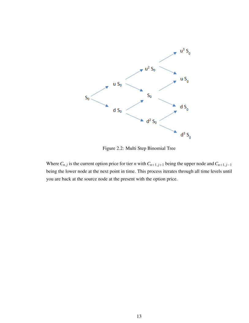
Figure 2.2: Multi Step Binomial Tree

Where Cn, j is the current option price for tier n with Cn+1, j+1 being the upper node and Cn+1, j−1

being the lower node at the next point in time. This process iterates through all time levels until

you are back at the source node at the present with the option price.

13

2.1 Formulation of the Binomial Option Pricing Model by

replicating portfolios

Let a portfolio contain ∆ shares of the stock and an amount B invested in risk-free bonds with

a present value of ∆s+B. We want the option payoff equal to the portfolio payoff ([6]). Value

of replicating portfolio at time h with stock price Sh is ∆Sh + erhB. At the two possible states,

Su = uS and Sd = dS the replicating portfolio must satisfy ([7]):

(∆uSeδh)+(Berh) = Cu,

(∆dSeδh)+(Berh) = Cd,

with δ being the dividend yield, Cu being the upper option node and Cd being the lower option

node. Then solving for ∆ and B:

Cu−∆uSeδh = Cd−∆dSeδh,

∆ = eδh(Cu−Cd

uS−dS), (2.1)

Berh = Cu−∆uSeδh, (2.2)

substituting (2.1) into (2.2) yields

Berh = Cu−uS(Cu−Cd)

uS−dS,

B = e−rh(uCd−dCu

u−d.

The cost of creating the option is the cash flow required to buy the shares and bonds ([7]):

∆S+B = e−rh[uCd−dCu

u−d+ e(r−δ )hCu−Cd

u−d],

= e−rh[Cue(r−δ )h−d

u−d+Cd

u− e(r−δ )h

u−d],

= e−rh[Cu p+Cd(1− p)],

arriving at the required equation.

14

2.2 Binomial model to the Trinomial model

One step in the trinomial tree can be seen as a combination of two steps of the binomial model,

either two up or down jumps or one of each. Taking equations from the binomial model and

applying two steps, Figure 2.3 shows the probabilities and the jump sizes for the Trinomial

model.

Figure 2.3: Binomial to Trinomial Formulation

Option prices were calculated using the trinomial tree with different values for the jump sizes

and probabilities depending on either CRR, RB and JR, and the equal probability tree for Google

between 23/04/2013 up to 20/12/2013 on a Call option with a strike price=1000. The volatility

used is the average of all the implied volatilities over the time of the contract at each discrete

daily time step. Plotted below in figure 2.4 are the trinomial trees calculated prices compared

to the market prices in the first row and the corresponding difference between the two on the

second row.

By figure 2.4, we can see that the equal-probability tree is closer to the market price than the

CRR and the RB and JR tree with an average difference of 2, compared to an average of 14 for

the CRR and RB and JR. Also on the difference plots of CRR and RB and JR, we notice the

15

Figure 2.4: Implied Google Call Option prices through the trinomial tree compared with market

prices

closer the option reaches maturity, the difference is approximately increasing. This could be due

to the increasing volatility over the time of the contract and only calculating the prices with a

constant volatility.

16

Chapter 3

Trinomial Tree

3.1 Pricing a European option through the Trinomial Tree

Solving the trinomial tree with the initial stock price (S0), number of time steps up to maturity

(n), strike price on the option (K), t treesize.m computes the option price with the choice of a

equal-probability tree, RB and JR tree and finally the CRR tree, Appendix (B).

The payoffs on the trinomial tree will be the leaf nodes comprising of 2n+1 elements as shown

below;

max(S0un−K,0)

max(S0un−1−K,0)...

max(S0u−K,0)

max(S0mn−K,0)

max(S0d−K,0)...

max(S0dn−1−K,0)

max(S0dn−K,0)

,

The values of u,m and d are pre-calculated along with the probabilities depending on what

trinomial tree is being solved. To discount these option payoffs back to present, two vectors

A and B with lengths 2n+ 1 and 2n− 1 respectively are created with assigning the payoffs to

vector A, then dynamically iterating back through n time steps with the calculation of each of

the nodes at each time level, while simultaneously making the vector shorter until we are back at

the present with one node being the option price. For each time level the vector B is computed

17

by;

Bi−1 = er·dt(puAi−1 + pmAi + pdAi+1)

dt = T/n,

pu + pm + pd = 1,

with k representing the time level and n being the number of iterations back to the present.

Clearing vector A with length 2(n−k)+1 and setting this vector equal to vector B. The current

vector B is not needed, so is cleared and a new vector B is created two elements shorter than the

previous vector A. These elements of B are computed again one time step closer to the present

being the option price at k equal to n. Plotted below in Figure 3.1 are the option prices, against

share price with a strike price of 25, σ being 0.25, time till maturity being a year with a risk-free

interest rate of 0.005.

Figure 3.1: European Call and Put Option Prices against Share price

When the stock price is equal to strike price, Figure 3.1 shows the option price for a call and a

put option are the same, also known as ’at the money’. When S > K the call option becomes ’in

the money’ with the put option becoming ’out of the money’, therefore the price of a call option

is increasing as the share price becomes deeper in the money. Vice versa for S < K as the put

option is now ’in the money’ and a call option being ’out of the money’.

18

3.2 Pricing an American option through the Trinomial Tree

American option contracts can be exercised at any point up to and including maturity, therefore

the iteration sequence back to the present needs to be modified by re-defining the payoff at every

node of the tree ([14]);

Calloptionpayo f f = max(Si, j−K,0),

Putoptionpayo f f = max(K−Si, j,0),

where,

Si, j = S0uNudNd mNm

with Nu +Nd +Nm = n, n being the time level in between the present and maturity. Each node

for each time level is computed by,

Cn, j = max(optionpayo f f ,e−r∆t [puCn+1, j+1 + pmCn+1, j + pdCn+1, j−1].

To solve for these changes we modify the matlab m file t treesize.m (Appendix B) by creating

a vector C the same size as vector A after transferring the values from vector B in the iteration.

The initial payoffs are calculated the same way, and then computing the stock prices for the

corresponding point in time by the up, middle and down jumps applied to the initial stock price.

This vector’s length will change with the point of time by 2(n− k)+1, with k representing the

point in time.

max(S0un−k−K,0)

max(S0un−k−1−K,0)...

max(S0u−K,0)

max(S0mn−k−K,0)

max(S0d−K,0)...

max(S0dn−k−1−K,0)

max(S0dn−k−K,0)

, (3.1)

the elements of vector A will be,

Ai = max(Ci,Ai).

The process repeats again one step closer to the present.

19

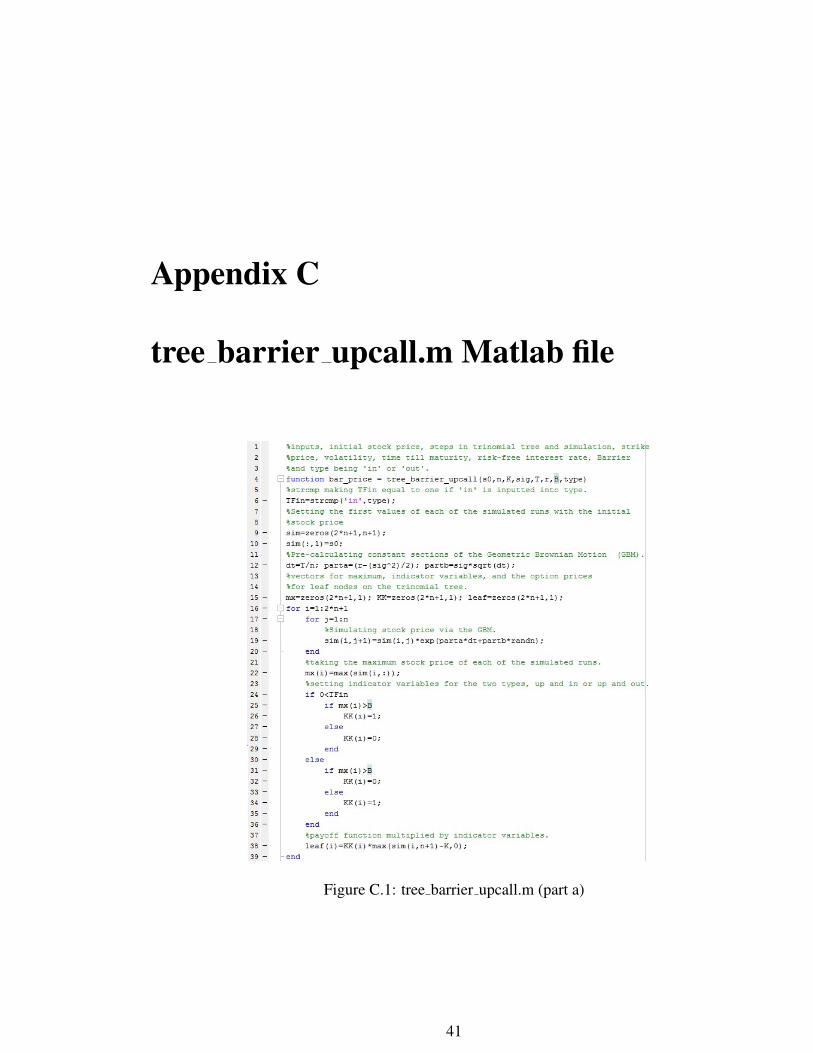
3.3 Pricing a Barrier option through the Trinomial Tree

A barrier option is a path-dependent option whose price is equal to that of a European option,

depending if the price crosses or doesn’t cross a barrier up to maturity, otherwise the payoff is

equal to zero. This is represented by an indicator variable ’I’ taking values 1 or 0 and multiplying

this variable by the payoff function for a European option. To use the trinomial tree to price such

an option, we simulate 2n+1 runs through the Geometric Brownian Motion (GBM), matching

the required leaf nodes on the trinomial tree;

Si = Si−1e∆t(µ−σ22 )+σ

√∆tε(i−1), i≥ 1.

∆t =Tn

Once the runs have been simulated the maximum or minimum of each run is taken depending on

whether the option is an up version or a down version with B > S0 or B < S0 respectively, with

the indicator variables. Once the indicator variables have been configured for each simulated

Table 3.1: Indicator Variables for Barrier Options

Up and Inmax0<S≤ST >B I=1

max0<S≤ST <B I=0

Up and Outmax0<S≤ST >B I=0

max0<S≤ST <B I=1

Down and Inmin0<S≤ST >B I=0

min0<S≤ST <B I=1

Down and Outmin0<S≤ST >B I=1

min0<S≤ST <B I=0

run, the payoffs of each run are computed by,

call payo f f s = I·max(ST −K,0),

put payo f f s = I·max(K−ST ,0),

20

ST being the final value of the corresponding simulated run. The payoffs being 2n+1 in length

these are simply plugged into the initial vector A from the Trinomial tree and iteratively dis-

counted back to the source node giving the final option price. Matlab file tree barrier upcall.m

is shown in Appendix (C). Plotted below in Figure 3.2 are the option prices of the different

barrier options while varying the barrier value, with inputs,

• S0 = 50,

• n = 250,

• K = 50,

• σ = 0.25,

• T = 1

• r = 0.005,

• dB = 0.1,m = 250.

Figure 3.2: Barrier Option Prices with varying barrier value

Two separate barrier vectors were used in Figure 3.2, one for the up version (top row of Figure

3.2) with the first barrier value being 50, increasing by 0.1 up to 75. The second still starting at

50 but decreasing by 0.1 down to 25 (bottom row of figure 3.2). One can see that for a up and out

21

option the price of the option is increasing as the barrier value increases, due to less simulated

runs crossing the barrier due to the volatility remaining constant. If the volatility was to increase

proportional to the increase in the barrier value, the option price would expect to approximately

maintain the same price. For the up and in barrier option, the price is decreasing due to the same

reasons. The put options on all barrier options increase or decrease more dramatically, than the

call option of the barrier values. This could be the time value of money in the call’s favour

against the put, therefore incorporating higher charges on put options as barrier value varies.

For the down and in, as the barrier moves further away from the initial stock price the option

becomes cheaper, again due to the constant volatility. Vice versa for the down and out barrier

option.

22

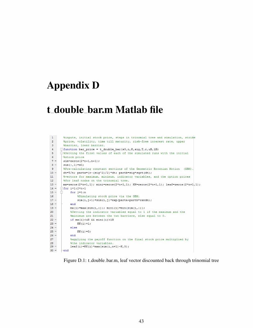
3.4 Pricing a Double Barrier Knockout option through the

Trinomial Tree

Extending the single barrier option to a double barrier can be beneficial for informed investors

betting on the price-movements of the security while still maintaining the same strike price on

a cheaper option[14]. A double barrier knockout option payoff is equal to that of a European

option payoff, if the maximum and the minimum of the underlying asset over the life of the

contract is between the two barriers. A slight modification on the calculation of the indicator

variables is needed to incorporate these double barriers. The payoffs are computed the same way

Table 3.2: Indicator Variables Double Barrier Knockout Option

Double Barrier Knockout Optionmax<uB and min>lB I=1

else I=0

as before and then discounted back through the trinomial tree to the source node giving the price

of the option contract. Plotted below in Figure 3.3 are the option prices against the difference

between the two barriers on the knockout option with inputs,

• S0 = 50,

• n = 250,

• K = 50,

• σ = 0.2,

• T = 1,

• r = 0.005,

• dB = 0.1 up to 25 away from S0 in both directions.

Figure 3.3 shows as the difference between the two barriers is increasing from the initial stock

price, the option price is increasing. This would be expected as the maximum and minimum

of each of the simulated runs up to maturity, are not breaching either of the two barriers giving

the European option payoff. Matlab file t double bar.m computes the price of a double barrier

knockout, Appendix (D).

23

Figure 3.3: Double Barrier Knockout Option

24

Chapter 4

The Greeks

The Greeks are partial derivatives with respect to the underlying parameter to see the sensitivity

of small changes in that parameter. Delta measures the rate of change of the option price with

respect to the underlying security ([15]), ∆ =∂V∂S

. Delta being between 0 and 1 for long position

and 0 and -1 for a short position, signifying the amount of stock to hold with respect to number

of option contracts in the portfolio. This idea is known as the Delta-Hedging rule. Delta can also

be seen as the probability of that option being ’in the money’ at maturity ([16]). Theta measures

the sensitivity of the value of option price given the passage of time, commonly divided by the

number of days in a year ([15]),θ =∂V∂ t

. Gamma measures the rate of change in the delta with

respect to the underlying security, therefore being a second order derivative, Γ =∂∆

∂S=

∂ 2V∂S2

([15]). Gamma is commonly used as an extension of the delta hedging rule allowing for a wider

range of movements in the underlying security, known as Delta-Gamma-Hedging rule.

25

4.1 Greeks via the Black-Scholes Model

The solution of the Black-Scholes model for a call option at a point in time till maturity (t) for

an underlying security (x) given by [18](p159-160),

c(t,x) = xN(d+(T − t,x))−Ke−r(T−t)N(d−(T − t,x)),

d±(τ,x) =1

σ√

τ[log(

xK)+(r± σ2

2)τ],

N(y) =1√2π

∫ y

−∞

e−Z22 dZ =

1√2π

∫∞

−ye−

Z22 dZ.

Taking partial derivatives of the above equation to show the value of the required Greek under

the input parameters of current stock price (x), time till expiration (τ), strike price (K), risk-free

interest rate (r) and the stocks volatility (σ ).

Delta

Cx(t,x) = N(d+(T − t,x)),

Theta

Ct(t,x) =−rKe−r(T−t)N(d−(T − t,x))− σx2√

T − tN′(d+(T − t,x)),

Gamma

Cxx(t,x) = N′(d+(T − t,x))∂

∂xd+(T − t,x),

=1

σx√

T − tN′(d+(T − t,x)).

Plotting the above equations in figure 4.1 for share prices between 0 up to 50 in increments of

0.1 and the time till maturity of a year in increments of 0.2. Strike price of 30 with a risk-free

interest rate of 0.005 and a σ of 0.2.

More than half of the shares are shown to be purchased when the share price crosses the strike

price, with holding all the shares with a delta of 1 when the option contract is ’deep in the

money’. Reflecting a less riskier portfolio and incurring a cheaper cost of buying shares if

the share price holds around the strike price, reflecting an uncertainty of the option maintain-

ing ’in the money’. Theta showing the option looses more value per the passage of time the

closer the option reaches maturity around the share price equalling the strike price. While loos-

ing less value as time reaches maturity with the option being ’in the money’ or ’out of the

money’. Gamma showing the rate of range of Delta being the greatest nearer maturity concen-

trated around the strike price on the option. This is seen with Delta’s biggest change when the

26

Figure 4.1: Delta, Theta and Gamma Greeks via the Black-Scholes model varying time till

maturity

share price crosses the strike price. Plotted in figure 4.2 are the same three Greeks but taking

a range of strike price values from 5 in increments of 5 up to 45 with all other variables kept

constant.

Figure 4.2: Delta, Theta and Gamma Greeks via the Black-Scholes model varying Strike Price

27

Can see that the option contract looses more value when crossing the strike price with the pas-

sage of time (Theta), however is proportional to the current share price. Also delta clearly show-

ing the greatest change when the share price goes through the strike price, shown by Gamma.

Figure 4.3 shows how the Greeks change up to maturity with all other variables kept constant,

with either the option being ’out of the money’, ’at the money’ or ’in the money’. Time till

maturity of a year, risk-free interest rate of 0.05, and a σ of 0.1 were used for figure 4.3.

Figure 4.3: Delta, Theta and Gamma Greeks via the Black-Scholes model up to maturity

Keeping all other variables constant, one can see that the delta decreases closer the option reach-

ing maturity. This is expected due to less time for the share price to vary, possibly coming ’out

of the money’. A lower probability of the option maturing ’in the money’ being represented by

the Delta. Option contracts still with a significant time till maturity loose more value over the

passage of time when they are ’out of the money’ than option contracts being ’in the money’.

However gradually gets reversed closer the option reaches maturity ending with ’in the money’

options loosing greater value than ’out of the money’ options. Gamma, again showing the rate

of change of Delta with respect to the underlying asset, has the greatest change with ’out of the

money’ options linked to a decreased probability (Delta) of the option maturing ’in the money’

the closer the option reaches maturity.

28

4.2 Delta and Gamma through the Trinomial Tree

Creating a function and denoting my trinomial tree by f (S,n,K,σ ,T,r), Delta and Gamma

Greek’s are calculated through the tree by[14](p8-9),

∆ =f (S+dS,n,K,σ ,T,r)− f (S,n,K,σ ,T,r)

dS,

Γ =f (S+dS,n,K,σ ,T,r)−2 f (S,n,K,σ ,T,r)+ f (S−dS,n,K,σ ,T,r)

dS2 ,

dS = Sσ√

T ,

• dS is chosen such that the amount is proportional to the volatility and the current share

price, while taking into consideration time till maturity.

Plotted in Figure 4.4 are the Delta and Gamma values against share price, via the trinomial tree

and the Black-Scholes model. From the figure we can clearly see the trinomial tree approxi-

mately follows the same values as the Black-Scholes model. This would be expected as both

methods are built on the assumption the stock price follows the Geometric Brownian Motion

(GBM), with assumed constant volatility up to maturity.

Figure 4.4: Delta and Gamma Greeks via the Trinomial tree and the Black-Scholes model

Done using matlab file g com.m, Appendix (E).

29

Chapter 5

Hedging Strategies

Investors like to diversify their risk against stock movements by going short on European call

options, while at the same time being long on the underlying asset. Or long on European put

option, while going short on the underlying asset. The amount of stock held is equal to the

Delta of the option multiplied by the number of option contracts purchased in the portfolio,

along with the multiple of lot size, (number of share’s the option contract gives right to buy/sell

at strike price at maturity). A portfolio with this characteristic is known to be delta-neutral,

the share price will vary leading up to maturity and in turn the Delta will change value. To

keep the portfolio delta-neutral, the underlying asset needs to be bought or sold appropriately

on the change of the delta leading up to maturity. Rebalancing the portfolio keeps the portfolio

more risk averse to small changes in the stock price. Ideally the number of rebalances would be

continuous, called self-financing portfolio but in practice is impossible due to transaction costs.

A high Gamma showing a high rate of change of Delta, indicates the portfolio becomes more

riskier the longer the time interval becomes between the portfolio rebalancing. The stock price

moving from S to S′ indicates the option price to move from C to C′, however moves to C′′, the

difference between C′′−C′ is the hedging error[19](p361). Fixing this error will allow for larger

price jumps in the share price, making the portfolio less riskier than just the delta-hedging rule,

extending on to the delta-gamma-hedging rule.

30

5.1 Delta-hedging rule

To begin the delta-hedging rule, an initial cost is incurred of setting up the portfolios positions.

Going long on the shares with a short European call option (lot size being a 100 shares), therefore

borrowing the initial cost minus the cost of the option contracts,

C0 = ∆0N100S0,

B0 = C0−N f0.

C and B being the cost an amount borrowed respectively, N the number of option contracts

and f being the price of the call option with ∆ being calculated via the trinomial tree. At each

rebalancing point (i) the cumulative cost and borrowed money being ([21]),

Ci = Ci−1er

252 +N100(∆i−∆i−1)Si,

Bi = N100∆iSi−N fi.

At maturity the option can be exercised if ST≥K giving the replication cost,

repcost = CT −N100K,

leading on to the gain after taking in to account the initial price of the option contracts,

netgain = f0Nerx

252 − repcost,

x being number days between initial purchase of option contract and maturity.

Call Option price data and stock price data was taken from the Bloomberg Terminals for Mi-

crosoft (MSFT) between 19/08/2013 up to 20/12/2013 with a strike price of 34, the delta-hedge

rule was applied to the data while rebalancing every day. The volatility used for the calculations

was the average of all the Implied Volatilities leading up to maturity. 10 option contracts were

purchased with a lot size of a 100 and a risk-free interest rate of 0.005, plotted in Figure 5.1 is

the cumulative cost, delta, stock price and the amount of money needed to borrow up to maturity

on the contract. Matlab file delta rebalance.m was used for calculations, Appendix (F).

The option matured in the money with a final stock price of 36.8 making the European call op-

tion ’in the money’, therefore exercisable with a strike price of 34. The cumulative cost of the

hedge was 34011 resulting in a replication cost of 11.0826. Giving final net value of -2.77. Such

a small loss in size, in comparison to the cost showing the delta-hedge rule eliminates more risk,

but in turn giving a lower return.

31

Figure 5.1: Delta-hedge rule, rebalancing every day

5.1.1 Delta-hedge rule across different companies

The same process was run again on Microsft (MSFT), Google (GOOG) and Apple (AAPL) each

with a variety of three strike prices, 10 option contracts with a risk-free interest rate of 0.005.

Following table shows key results along with net loss/gain.

Table 5.1: Delta-hedging rule comparison of companies

MSFT AAPL

ST 36.8 549.02

K 34 35 36 450 500 550

CT 34,027 34,723 29,446 513,770 525,280 245,330

Rep Cost 26.7219 -277.419 6,553.5 63,774 2528.1 -257,030

Net Value -18.4073 285.5298 6557.2 -63,085 -24,924 257,200

Net Value/CT -0.054 0.822 22.27 -12.28 -4.74 104.83

Table 5.1 showing the delta-hedge rule eliminating a lot of potential loss when ST hasn’t crossed

the strike price, while taking a nice return on options maturing ’in the money’. Seen with MSFT

with strike price of 36 and GOOG with a strike price of 1100, taking returns of 22.27% and

32

GOOG

ST 1100.6

K 900 1000 1100

CT 922,310 998,240 329,040

Rep cost 22,310 -1759.2 -770,960

Net value -21,994 1836.3 770,980

Net value/CT -2.38 0.184 234.311

234.311% respectively. Compared with loss return of 0.054% and 2.38% for MSFT and GOOG

respectively for the lower strike prices. Signifying option contracts with higher strike price in

the future become cheaper, reflecting a lower probability that the contract will mature ’in the

money’. This is shown by a small difference between the replication cost and net value for the

higher strike prices.

33

5.2 Rebalancing under delta tolerance

Instead of rebalancing every data point (daily), modifying the delta rebalance.m (Appendix F),

with an additional input for delta tolerance. Only rebalancing if the absolute value of the change

between the delta of the previous rebalance, and the current delta is greater than the delta toler-

ance. If the tolerance is not met, leave the holding of shares the same. Doing this will reduce

the amount of transaction costs incorporated over the life of the option, however may not give

a higher gain due to the increased volatility closer to the option reaching maturity. More fre-

quent rebalancing would be required to hedge more of the investors risk, this could be done by

the delta tolerance decreasing closer the option reaches maturity. Better still make the decrease

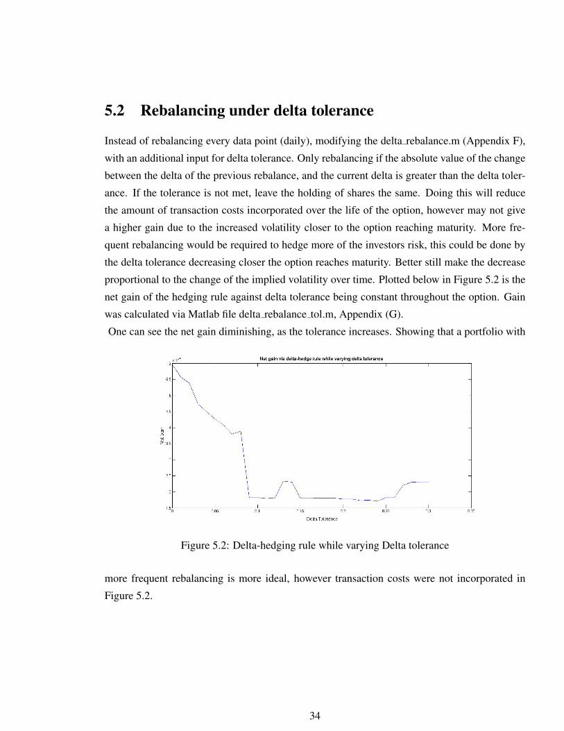
proportional to the change of the implied volatility over time. Plotted below in Figure 5.2 is the

net gain of the hedging rule against delta tolerance being constant throughout the option. Gain

was calculated via Matlab file delta rebalance tol.m, Appendix (G).

One can see the net gain diminishing, as the tolerance increases. Showing that a portfolio with

Figure 5.2: Delta-hedging rule while varying Delta tolerance

more frequent rebalancing is more ideal, however transaction costs were not incorporated in

Figure 5.2.

34

5.3 Delta-hedging including Transaction Costs

Buying and selling stocks on the market to rebalance the portfolio incurs transaction costs.

Either a fixed charge per share, a percentage of shares bought or sold, or just a flat fee regardless

of the number of shares ([20]). At each rebalancing point, additional charges are included in the

cumulative cost of the delta-hedge,

Ci = Ci−1er

252 +N100(∆i−∆i−1)Si + pSiN100(∆i−∆i−1),

where (p) is the percentage charge of the transaction, only being applied to number of shares

purchased keeping the portfolio delta-neutral. More additional costs occur in practice, the dif-

ference between buying and selling from the broker, known as the bid-ask spread. Stamp duty,

tax and other over night financing costs occur with the holding of your securities. More so-

phisticated pricing techniques of these options are required to give a more accurate and realistic

option price, with additional extension on to allowing the volatility to vary up to maturity on the

option contract.

35

Chapter 6

Conclusion

The equal probability trinomial tree being the most accurate against market prices, even with

assumed constant volatility with an average difference of 2 between the trinomial tree option

price and the market prices. Using the equal probability tree throughout for further calculations

due to the increased accuracy compared to CRR and JR. Using this trinomial tree for the calcu-

lation of the delta and gamma of an option, allows us to rebalance an option contract with the

underlying asset to minimize the risk to the market. This is known as the delta-hedge rule where

rebalancing is carried out on the portfolio to eliminate risk, however continuous rebalancing is

infeasible due to additional transaction costs. Further extension of the delta-hedging rule would

be the delta-gamma hedging rule, rebalancing the holding of the traded option with respect to

the delta on the underlying asset. Therefore a delta-gamma hedging rule allows for a larger

price movement in the underlying asset between rebalancing points. Extending this again by a

delta-gamma-vega hedging rule, incorporating an additional option in the portfolio taking ad-

vantage of the volatility between rebalancing points. Additionally transaction cost are incurred

from the broker, bid-ask spread. Buying and selling of the underlying asset are not of the same

value. So two share price vectors will need to be included in the calculations, one for buying the

underlying asset and one for selling. Doing this will include the brokers transaction cost as well

as adding the fixed charge percentage on the rebalancing transaction.

36

Chapter 7

Recommendations and Further Work

7.1 Implied Trinomial Tree

The trinomial tree assumes constant volatility throughout, an extension of this being the implied

trinomial tree. Where the implied volatilities are computed through the market prices, and the

volatility smile is interpolated across the tree varying the size of the jumps and time between the

jumps. Figure 7.1 shows a constant trinomial tree and an implied trinomial tree.

Figure 7.1: Trinomial tree and an Implied trinomial tree ([22])

37

7.2 Further Hedging Techniques

Delta-Gamma hedging rule rebalances the holding of option contracts between the delta-rebalance

points. ”What is required is a position in an instrument such as an option that is not linearly de-

pendent on the underlying asset” ([19],p363). Letting Γ being the Gamma of a delta-neutral

portfolio and Γτ be the Gamma of a traded option, then the the overall Gamma of the portfolio

with wτ holding of the option contract being ([19],p363),

wτΓτ +Γ (7.1)

holding − Γ

Γτof the option contract will in turn make the portfolio gamma-neutral, but the port-

folio may not be delta-neutral anymore, so a rebalancing of the underlying asset is needed.

Vega is an another partial derivative of the Black-Scholes equation with respect to volatility,

ν = ∂V∂σ

([15]). Having a holding of − ν

ντin a traded option will make the portfolio Vega neu-

tral, a portfolio cant be gamma and Vega neutral unless another traded option is bought into the

portfolio ([19],p365). Solving simultaneously the amount of options to hold for the Gamma and

Vega making the respective partial derivative equal to zero on the portfolio. Correspondingly

buying or selling the underlying asset to maintain delta neutrality, in turn made the portfolio

delta-gamma-vega neutral.

38

Appendix A

my impvol.m Matlab file

Figure A.1: my impvol.m

39

Appendix B

t treesize.m Matlab file

Figure B.1: t treesize.m

40

Appendix C

tree barrier upcall.m Matlab file

Figure C.1: tree barrier upcall.m (part a)

41

Figure C.2: tree barrier upcall.m (part b)

42

Appendix D

t double bar.m Matlab file

Figure D.1: t double bar.m, leaf vector discounted back through trinomial tree

43

Appendix E

g com.m Matlab file

Figure E.1: g com.m

44

Appendix F

delta rebalance.m Matlab file

Figure F.1: delta rebalance.m (part a)

45

Figure F.2: delta rebalance.m (part b)

46

Appendix G

delta rebalance tol.m Matlab file

Figure G.1: delta rebalance tol.m (part a)

47

Figure G.2: delta rebalance tol.m (part b)

48

Appendix H

Background and Project Plan

Ciaran Cox (1115773)Jacques Furter

Pricing options with trinomial trees

Aims and Objectives

• To understand the pricing of options and implement algorithms in Matlab programming.

• To compute prices of barrier options by trinomial trees and compare the price with the

Black-Scholes equation from Mathematical Finance (MA3667) module assignment.

• To understand the concepts of an Implied Trinomial Tree (ITT).

• Use trinomial trees to calculate the option greeks.

Project Plan

I will begin my project with a brief history of option pricing and some of the key breakthroughs

in mathematical finance, along with the definition of an option contract along with its features

and properties. Then I will talk about the binomial option pricing model by Cox,Ross and Ru-

binstein (CRR)(1979) and its variant by Rendleman-Barter (RB) and Jarrow-Rudd (JR)(1979).

Then extending the idea of a binomial model to a trinomial model by Boyle (1986) and imple-

ment algorithms in Matlab to formulate a trinomial tree and calculate the price of barrier options.

I will also mention the trinomial tree with a diffusion parameter by Kamrad and Ritchken (1991).

Black-Scholes equation by Black and Scholes (1973) will be covered and compared with trino-

mial trees. Also comparing the price a barrier option valued by the trinomial tree along with

49

the price of the same option calculated by the Black-Scholes equation from the Mathematical

Finance (MA3667) module. The family of option greeks will be covered and a few of them

calculated through the trinomial tree.

I will then extend from the Black-Scholes equation and trinomial tree which assumes constant

volatility to the Implied Trinomial Tree by Derman, Kani, and Chriss (1996). Relevant option

price data will also need to be collected either via the Bloomberg terminals or Datastream termi-

nals for the calculation of the implied volatility at different time points throughout the implied

trinomial tree, not all option price data will be available therefore interpolation will be required

to match the volatilities to the volatility smile.

Gant Chart showing the project layout is in Appendix 1.

Background

Introduction

An option is a type of contract that gives the holder the right to, but not obligation to buy (call)

or sell (put) an underlying asset or instrument at a specified strike price on or before a specified

date.

• European option can only be exercised at the expiration date.

• American option can be exercised at any time between the purchase date and the expiration

date.

• Bermuda option can only be exercised at certain times leading up to expiration date, which

are discussed in the option contract.

Pricing of these options has been around for a while, but in 1973, Fisher Black and Myron

Scholes published a paper, ’The Pricing of Options and Corporate Liabilities’.[1] They had an

idea to hedge the option by buying or seeling the underlying asset in such a way to eliminate

risk. With this they derived a stochastic partial differential equation which estimates the price of

the option over time.The Black-Scholes equation let to a boom in finance and more specifically

option trading around the world.[8]

Overiew

50

In the following I cover a brief overview of where I’m taking my project and what areas of

option pricing I’ll be covering. Firstly looking at the binomial option pricing model which was

the first of its kind by Cox, Ross and Rubinstein (CRR)(1979)[1], followed by the formulation

of the model by replicating portfolios. With an extension of the model to 3 states (trinomial)

first introduced by Boyle (1986)[5]. Concluding on Implied Trinomial Trees which is a further

extension by allowing for changing volatility over the time period of the asset by matching the

implied volatilities with the volatility smile.[10]

Binomial Option Pricing Model

Another method for a pricing a stock option is a lattice model, which divides time from now up

to expiration into N discrete time periods with each point going to 2 possible states (Binomial)

or 3 possible states (Trinomial) all the way up to expiration date where the expected payoff’s are

calculated. Then discounting yourself back through the tree until you reach the option price at

the source node.

The first lattice model was the Binomial Option Pricing Model (BOPM) By Cox, Ross and

Rubinstein (CRR)(1979)[1]. From the source node the underlying asset either goes up with

probability p or down with probability 1− p. This process repeats until you reach the expiration

date with all the possible stock outcomes. The expected payoffs are then calculated at expiration

by:

CallOption = max{ST −K,0},

PutOption = max{K−ST ,0}.

ST being the stock price at expiration (T ) with K being the strike price on the option. Expected

payoffs are then discounted back through the tree by risk-neutral probabilities until your back at

the source node and reached the option price. Figure 1 below shows the Binomial Tree.

Figure 1 shows a non-recombining tree and a recombining tree. It is computationally efficient to

have a recombining tree over a non-recombining tree, because if the tree recombines, there are

only N + 1 nodes at stage N, whereas there will be 2N nodes at stage N on a non-recombining

tree. To make the tree recombine CRR[1] made ud = 1, making an up jump followed by a down

jump equal to your original position. There is 3 parameters in Binomial model u,d, and p, we

therefore need 3 equations to solve for the parameters. First equation comes from matching

the expectation of return on the asset in a risk-neutral world. The Second from matching the

51

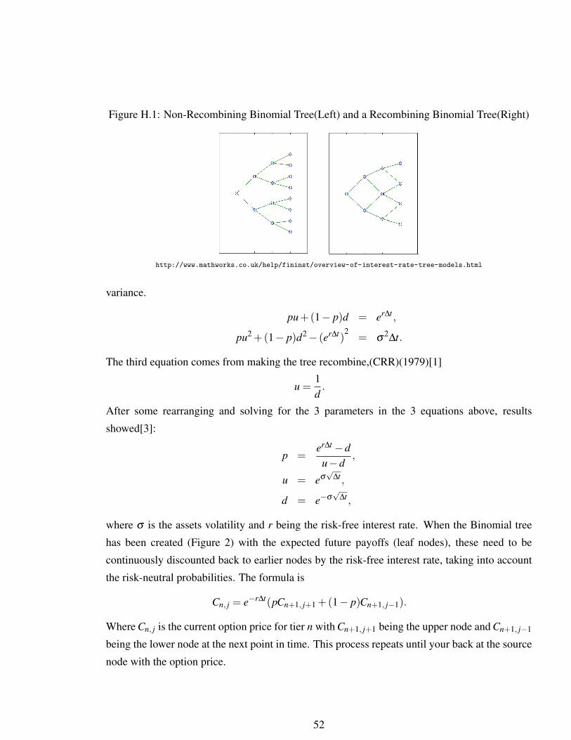
Figure H.1: Non-Recombining Binomial Tree(Left) and a Recombining Binomial Tree(Right)

http://www.mathworks.co.uk/help/fininst/overview-of-interest-rate-tree-models.html

variance.

pu+(1− p)d = er∆t ,

pu2 +(1− p)d2− (er∆t)2

= σ2∆t.

The third equation comes from making the tree recombine,(CRR)(1979)[1]

u =1d.

After some rearranging and solving for the 3 parameters in the 3 equations above, results

showed[3]:

p =er∆t−du−d

,

u = eσ√

∆t ,

d = e−σ√

∆t ,

where σ is the assets volatility and r being the risk-free interest rate. When the Binomial tree

has been created (Figure 2) with the expected future payoffs (leaf nodes), these need to be

continuously discounted back to earlier nodes by the risk-free interest rate, taking into account

the risk-neutral probabilities. The formula is

Cn, j = e−r∆t(pCn+1, j+1 +(1− p)Cn+1, j−1).

Where Cn, j is the current option price for tier n with Cn+1, j+1 being the upper node and Cn+1, j−1

being the lower node at the next point in time. This process repeats until your back at the source

node with the option price.

52

Figure H.2: Multi-Step Binomial Tree

http://investexcel.net/binomial-option-pricing-excel/

Formulation of the Binomial Option Pricing Model by replicating portfolios

Let a portfolio contain ∆ shares of the stock and an ammount B invested in risk-free bonds with

a present value of ∆s+B. We want the option payoff = portfolio payoff.[6] Value of replicating

portfolio at time h with stock price Sh is ∆Sh + erhB. At Sh = uS and Sh = dS the replicating

portfolio must satisfy[7]:

(∆uSeδh)+(Berh) = Cu,

(∆dSeδh)+(Berh) = Cd,

with δ being the dividend yield, Cu being the upper option node and Cd being the lower option

node. Then solving for ∆ and B:

Cu−∆uSeδh = Cd−∆dSeδh,

∆ = eδh(Cu−Cd

uS−dS), (H.1)

Berh = Cu−∆uSeδh, (H.2)

substituting eq(1) into eq(2) yields:

Berh = Cu−uS(Cu−Cd)

uS−dS,

B = e−rh(uCd−dCu

u−d.

53

The cost of creating the option is the cash flow required to buy the shares and bonds[7]:

∆S+B = e−rh[uCd−dCu

u−d+ e(r−δ )hCu−Cd

u−d],

= e−rh[Cue(r−δ )h−d

u−d+Cd

u− e(r−δ )h

u−d],

= e−rh[Cu p+Cd(1− p)].

Trinomial Model

The Trinomial model is an extension of the Binomial model. but taking an additional path at

each node of the stock price staying the same. This was first introduced by Boyle (1986) [5].

The foundations of the model are similar in the fact that the first two moments are matched

but with the first two moments of the Geometric Brownian Motion (GBM)[14], which behaves

similar to stock price movements.

E[S(ti+1)|S(ti)] = er∆tS(ti),

Var[S(ti+1)|S(ti)] = ∆tS(ti)2σ

2,

ud = 1.

The last constraint is needed to make the tree recombine, solving for the above equations

yields[14]:

u = eσ√

2∆t ,

v = e−σ√

2∆t ,

with the transition probabilities being:

pu = (e

r∆t2 − e−σ

√∆t2

eσ

√∆t2 − e−σ

√∆t2

)2,

pd = (eσ

√∆t2 − e

r∆t2

eσ

√∆t2 − e−σ

√∆t2

)2,

pm = 1− pu− pd.

The same discounting method is used from the Binomial model just extended to the trinomial

model:

Cn, j = e−r∆t(puCn+1, j+1 + pmCn+1, j + pdCn+1, j−1).

54

Figure H.3: Trinomial Tree Example

http:

//www.24-something.com/2011/03/07/how-to-create-trinomial-option-pricing-trees-with-excel-applescripts/

This process keeps repeating until back at the source node just like the Binomial Model. Figure

3 below shows an example of a trinomial tree with the blue being the stocks price with the option

price beneath.

Implied Trinomial Trees (ITT)

Implied trees allows for changing volatility between nodes by extracting an implied evolution

for the stock prices in equilibrium from market prices of liquid standard options on the underly-

ing stock.[2] Making implied trees an extension to the Black-Scholes equation which assumes

volatility is constant. A couple of new concepts are needed for the calculation of ITT, Arrow-

Debreu prices and the volatility smile.

Arrow-Debreu prices are the sum of the product of the risklessly discounted transition proba-

bilities over all paths starting in the root of the tree and leading to node (n, i), with n being the

nth time level and i being the highest node on that level. [10]

The Volatility Smile is the plot of implied volatility against varying strike prices as shown in

figure 4 below. ‘In the money’ meaning the option is worth something, ‘at the money’ being the

option is at the strike price and ‘out of the money’ meaning the option is worthless.

There is also a reverse skew and forward skew also known as the volatility smirk. In the reverse

skew pattern the implied volatility’s are higher at lower strike prices than the implied volatility at

higher strike prices. More frequently appears for longer term equity options and index options.

[11] In the forward skew pattern, the implied volatility for lower strike prices are lower than the

implied volatility at higher strike prices, commonly seen for options in the commodities market.

55

Figure H.4: Volatility Smile

http://www.investopedia.com/terms/v/volatilitysmile.asp

[11]

The Implied trinomial tree desires the following properties to model the underlying price cor-

rectly [10].

1. Reproduces correctly the volatility smile.

2. Is risk neutral.

3. Uses transition probabilities from the interval (0,1).

The study of implied trinomial trees is currently a work in progress.

56

Bibliography

[1] Black, Fischer; Myron Scholes (1973). The Pricing of Options and Corporate Liabilities.

Journal of Political Economy 81 (3): 637654. doi:10.1086/260062. [1] (Black and Scholes’

original paper.)

[2] MacKenzie, Donald (2006). An Engine, Not a Camera: How Financial Models Shape

Markets. Cambridge, MA: MIT Press. ISBN 0-262-13460-8.

[3] John C. Cox, Stephen A. Ross, and Mark Rubinstein. 1979. Option Pricing: A Simplified

Approach. Journal of Financial Economics 7: 229-263.

[4] http://www.goddardconsulting.ca/option-pricing-binomial-index.html

[5] P. Boyle, Option Valuation Using a Three-Jump Process, International Options Journal 3,

7-12 (1986).

[6] Professor P.A.Spindt Binomial Option Pricing

[7] https://www.google.co.uk/url?sa=t&rct=j&q=&esrc=s&source=web&cd=

3&ved=0CDgQFjAC&url=http%3A%2F%2Fwww2.fiu.edu%2F~dupoyetb%2FAdvanced_

Risk_Mgt%2Flectures%2Fweek%25201.ppt&ei=IPWDUu-gMMXIhAev8oCQDg&usg=

AFQjCNEOr7-1rmnXwdsiVze2JeAMszww2A&bvm=bv.56343320,d.ZG4&cad=rja

[8] P. Clifford, O. Zaboronski. Pricing Options Using Trinomial Trees (2008)

[9] E. Derman, I. Kani, N.Chriss. Implied Trinomial Trees of the Volatility Smile (1996)

[10] P.Cizek, K.Komorad Implied Trinomial Trees SFB 649 Discussion Paper (2005-007)

[11] http://www.theoptionsguide.com/volatility-smile.aspx

57

Appendix 1: Gant Chart for Pricing Options with Trinomial Trees Major Project

58

Bibliography

[1] John C. Cox, Stephen A. Ross, and Mark Rubinstein. 1979. Option Pricing: A Simplified

Approach. Journal of Financial Economics 7: 229-263.

[2] E. Derman, I. Kani, N.Chriss. Implied Trinomial Trees of the Volatility Smile (1996)

[3] http://www.goddardconsulting.ca/option-pricing-binomial-index.html

[4] F.Black and M.Scholes. The Pricing of Options and Corporate Liabilities The Journal of

Political Economy, Vol. 81, No. 3 (May - Jun., 1973), pp. 637-654

[5] P.Date and S.Virmani MA3667:Mathematical and Computational Finance Assignment

[6] Professor P.A.Spindt Binomial Option Pricing

[7] https://www.google.co.uk/url?sa=t&rct=j&q=&esrc=s&source=web&cd=

3&ved=0CDgQFjAC&url=http%3A%2F%2Fwww2.fiu.edu%2F~dupoyetb%2FAdvanced_

Risk_Mgt%2Flectures%2Fweek%25201.ppt&ei=IPWDUu-gMMXIhAev8oCQDg&usg=

AFQjCNEOr7-1rmnXwdsiVze2JeAMszww2A&bvm=bv.56343320,d.ZG4&cad=rja

[8] MacKenzie, Donald (2006). An Engine, Not a Camera: How Financial Models Shape

Markets. Cambridge, MA: MIT Press. ISBN 0-262-13460-8.

[9] Ross, Sheldon.M (2007). ”10.3.2”. Introduction to Probability Models

[10] http://en.wikipedia.org/wiki/Geometric_Brownian_motion

[11] Wilmott, Paul (2006). ”16.4”. Paul Wilmott on Quantitative Finance (2 ed.).

[12] Gatheral, J, (2006). The volatility surface: a practitioners guide, Wiley.

[13] http://en.wikipedia.org/wiki/Stochastic_volatility

59

[14] P. Clifford, O. Zaboronski. Pricing Options Using Trinomial Trees (2008)

[15] Haug, Espen Gaardner (2007). The Complete Guide to Option Pricing Formulas. McGraw-

Hill Professional. ISBN 9780071389976. ”ISBN 0-07-138997-0”

[16] http://en.wikipedia.org/wiki/Greeks_(finance)

[17] http://investexcel.net/binomial-option-pricing-excel/

[18] Shreve, Steven.E Stochastic Calculus for Finance 2, Continious Time models

[19] John.C.Hull Options, Futures, and other derivatives, (7th ed.)

[20] Chi Lee Option Pricing in the Presence of Transaction Costs

[21] Prof. Yuh-Dauh Lyuu, National Taiwan University (2007) Delta Hedge

[22] E. Derman, I. Kani and N. Chriss Implied Trinomial Trees of the Volatility Smile (1996).

60