DISSIPATIVE QUANTUM MOLECULAR DYNAMICS IN GASES AND CONDENSEDMEDIA: A DENSITY MATRIX TREATMENT

By

ANDREW S. LEATHERS

A DISSERTATION PRESENTED TO THE GRADUATE SCHOOLOF THE UNIVERSITY OF FLORIDA IN PARTIAL FULFILLMENT

OF THE REQUIREMENTS FOR THE DEGREE OFDOCTOR OF PHILOSOPHY

UNIVERSITY OF FLORIDA

2009

1

c© 2009 Andrew S. Leathers

2

To my grandfather,

William F. Leathers

3

ACKNOWLEDGMENTS

I would like to thank my advisor, Dr. David Micha, for his guidance and great

patience. I would also like to thank both the Department of Chemistry and the Quantum

Theory Project for providing a wonderful environment for study for the past years.

I would like to thank my parents, Steven and Marilyn Leathers for their support.

4

TABLE OF CONTENTS

page

ACKNOWLEDGMENTS . . . . . . . . . . . . . . . . . . . . . . . . . . . . . . . . . 4

LIST OF TABLES . . . . . . . . . . . . . . . . . . . . . . . . . . . . . . . . . . . . . 8

LIST OF FIGURES . . . . . . . . . . . . . . . . . . . . . . . . . . . . . . . . . . . . 9

ABSTRACT . . . . . . . . . . . . . . . . . . . . . . . . . . . . . . . . . . . . . . . . 12

CHAPTER

1 INTRODUCTION . . . . . . . . . . . . . . . . . . . . . . . . . . . . . . . . . . 14

1.1 The Reduced Density Matrix . . . . . . . . . . . . . . . . . . . . . . . . . 141.2 Alternative Methods . . . . . . . . . . . . . . . . . . . . . . . . . . . . . . 161.3 Our Method . . . . . . . . . . . . . . . . . . . . . . . . . . . . . . . . . . . 161.4 Two State Vibrational Relaxation . . . . . . . . . . . . . . . . . . . . . . . 161.5 Vibrational and Electronic Relaxation . . . . . . . . . . . . . . . . . . . . 171.6 Direct and Indirect Electron Transfer . . . . . . . . . . . . . . . . . . . . . 171.7 Outline of Dissertation . . . . . . . . . . . . . . . . . . . . . . . . . . . . . 17

2 DENSITY MATRIX EQUATION WITH DELAYED DISSIPATION . . . . . . 20

2.1 Introduction . . . . . . . . . . . . . . . . . . . . . . . . . . . . . . . . . . . 202.2 Liouville Equation for Reduced Density Matrix . . . . . . . . . . . . . . . 202.3 A Master Equation . . . . . . . . . . . . . . . . . . . . . . . . . . . . . . . 22

2.3.1 The Interaction Picture . . . . . . . . . . . . . . . . . . . . . . . . . 222.3.2 Projection Operator Formalism . . . . . . . . . . . . . . . . . . . . 232.3.3 A Master Equation . . . . . . . . . . . . . . . . . . . . . . . . . . . 252.3.4 Fast Dissipation Limits . . . . . . . . . . . . . . . . . . . . . . . . . 262.3.5 Diadic Formulation . . . . . . . . . . . . . . . . . . . . . . . . . . . 27

2.4 Quantum-Classical Treatment . . . . . . . . . . . . . . . . . . . . . . . . . 272.4.1 The Wigner Transform . . . . . . . . . . . . . . . . . . . . . . . . . 272.4.2 Partial Wigner Transform . . . . . . . . . . . . . . . . . . . . . . . 292.4.3 Quantum-Classical Treatment with Dissipation . . . . . . . . . . . . 31

3 QUANTUM-CLASSICAL TREATMENT . . . . . . . . . . . . . . . . . . . . . 32

3.1 Introduction . . . . . . . . . . . . . . . . . . . . . . . . . . . . . . . . . . . 323.2 Dissociation of NaI . . . . . . . . . . . . . . . . . . . . . . . . . . . . . . . 323.3 Effect of Initial Conditions . . . . . . . . . . . . . . . . . . . . . . . . . . . 34

4 NUMERICAL METHOD . . . . . . . . . . . . . . . . . . . . . . . . . . . . . . 44

4.1 A Runge-Kutta Method for Integro-Differential Equations . . . . . . . . . 444.1.1 Volterra Integral Equations . . . . . . . . . . . . . . . . . . . . . . . 454.1.2 Volterra Integro-Differential Equations . . . . . . . . . . . . . . . . 47

5

4.1.3 Order Conditions . . . . . . . . . . . . . . . . . . . . . . . . . . . . 504.2 Implicit Formulation . . . . . . . . . . . . . . . . . . . . . . . . . . . . . . 524.3 Test System . . . . . . . . . . . . . . . . . . . . . . . . . . . . . . . . . . . 534.4 Scaling and Limitations . . . . . . . . . . . . . . . . . . . . . . . . . . . . 564.5 The Memory Time . . . . . . . . . . . . . . . . . . . . . . . . . . . . . . . 574.6 Conclusion . . . . . . . . . . . . . . . . . . . . . . . . . . . . . . . . . . . . 59

5 VIBRATIONAL RELAXATION OF ADSORBATES ON METAL SURFACES 64

5.1 Introduction . . . . . . . . . . . . . . . . . . . . . . . . . . . . . . . . . . . 645.2 Model Details . . . . . . . . . . . . . . . . . . . . . . . . . . . . . . . . . . 645.3 The Correlation Function . . . . . . . . . . . . . . . . . . . . . . . . . . . 675.4 Results . . . . . . . . . . . . . . . . . . . . . . . . . . . . . . . . . . . . . . 685.5 Conclusions . . . . . . . . . . . . . . . . . . . . . . . . . . . . . . . . . . . 69

6 ELECTRONIC AND VIBRATIONAL RELAXATION . . . . . . . . . . . . . . 80

6.1 Introduction . . . . . . . . . . . . . . . . . . . . . . . . . . . . . . . . . . . 806.2 Model Details . . . . . . . . . . . . . . . . . . . . . . . . . . . . . . . . . . 806.3 Primary Region . . . . . . . . . . . . . . . . . . . . . . . . . . . . . . . . . 816.4 Secondary Region . . . . . . . . . . . . . . . . . . . . . . . . . . . . . . . . 846.5 Unperturbed Dynamics . . . . . . . . . . . . . . . . . . . . . . . . . . . . . 866.6 Results With a Pulse . . . . . . . . . . . . . . . . . . . . . . . . . . . . . . 866.7 Conclusion . . . . . . . . . . . . . . . . . . . . . . . . . . . . . . . . . . . . 87

7 ELECTRONICALLY NON-ADIABATIC DYNAMICS OF AG3SI(111):H . . . . 92

7.1 Introduction . . . . . . . . . . . . . . . . . . . . . . . . . . . . . . . . . . . 927.2 Model Details . . . . . . . . . . . . . . . . . . . . . . . . . . . . . . . . . . 927.3 Correlation Function . . . . . . . . . . . . . . . . . . . . . . . . . . . . . . 957.4 Direct Excitation . . . . . . . . . . . . . . . . . . . . . . . . . . . . . . . . 95

7.4.1 Initial Dynamics . . . . . . . . . . . . . . . . . . . . . . . . . . . . . 957.4.2 Photoinduced Dynamics . . . . . . . . . . . . . . . . . . . . . . . . 96

7.5 Indirect Excitation . . . . . . . . . . . . . . . . . . . . . . . . . . . . . . . 977.5.1 Initial Dynamics . . . . . . . . . . . . . . . . . . . . . . . . . . . . . 987.5.2 Photoinduced Dynamics . . . . . . . . . . . . . . . . . . . . . . . . 997.5.3 Memory Time . . . . . . . . . . . . . . . . . . . . . . . . . . . . . . 99

7.6 Conclusions . . . . . . . . . . . . . . . . . . . . . . . . . . . . . . . . . . . 101

8 CONCLUSION . . . . . . . . . . . . . . . . . . . . . . . . . . . . . . . . . . . . 118

8.1 Vibrational Relaxation . . . . . . . . . . . . . . . . . . . . . . . . . . . . . 1188.2 Electronic and Vibrational Relaxation . . . . . . . . . . . . . . . . . . . . 1198.3 Program Development . . . . . . . . . . . . . . . . . . . . . . . . . . . . . 1198.4 Future Work . . . . . . . . . . . . . . . . . . . . . . . . . . . . . . . . . . . 119

APPENDIX

6

A PROGRAM DETAILS . . . . . . . . . . . . . . . . . . . . . . . . . . . . . . . . 121

A.1 Overview . . . . . . . . . . . . . . . . . . . . . . . . . . . . . . . . . . . . 121A.2 Model Specific Functions . . . . . . . . . . . . . . . . . . . . . . . . . . . . 121A.3 Input And Output Files . . . . . . . . . . . . . . . . . . . . . . . . . . . . 122

REFERENCES . . . . . . . . . . . . . . . . . . . . . . . . . . . . . . . . . . . . . . . 124

BIOGRAPHICAL SKETCH . . . . . . . . . . . . . . . . . . . . . . . . . . . . . . . . 128

7

LIST OF TABLES

Table page

3-1 Parameters for the NaI model. . . . . . . . . . . . . . . . . . . . . . . . . . . . 35

4-1 Number of equalities to be satisfied for a given order of the Runge-Kutta method 59

4-2 Highest attainable order of an explicit Runge-Kutta method for a given m . . . 59

4-3 Minimum m needed to attain a given order p . . . . . . . . . . . . . . . . . . . 59

4-4 Example coefficients . . . . . . . . . . . . . . . . . . . . . . . . . . . . . . . . . 63

5-1 Frequencies and coupling parameters . . . . . . . . . . . . . . . . . . . . . . . . 70

6-1 Parameters for the ground and excited state potentials . . . . . . . . . . . . . . 89

6-2 Parameters for secondary region . . . . . . . . . . . . . . . . . . . . . . . . . . . 89

6-3 Parameters for the heat diffusion equations . . . . . . . . . . . . . . . . . . . . . 89

7-1 Parameters for the chosen transitions in Ag3Si(111):H . . . . . . . . . . . . . . . 101

8

LIST OF FIGURES

Figure page

1-1 Delayed dissipation between the primary region (P) and the secondary region(S). There is an excitation from the ground state (g) in the P region, then thereare interactions between the excited states (e) and the secondary region duringtimes t and t′ . . . . . . . . . . . . . . . . . . . . . . . . . . . . . . . . . . . . . 19

3-1 Potential curves for the NaI model . . . . . . . . . . . . . . . . . . . . . . . . . 36

3-2 Populations for the orbit and grid initial conditions . . . . . . . . . . . . . . . . 37

3-3 Real part of the coherence for the orbit and grid initial conditions . . . . . . . . 38

3-4 Imaginary part of the coherence for the orbit and grid initial conditions . . . . . 38

3-5 Initial form of the phase space for the grid initial conditions . . . . . . . . . . . 39

3-6 Initial form of the phase space for the orbit initial conditions . . . . . . . . . . . 39

3-7 Final form of the phase space for the grid initial conditions . . . . . . . . . . . . 40

3-8 Final form of the phase space for the orbit initial conditions . . . . . . . . . . . 41

3-9 Average P and σP for orbit and grid initial conditions, along with full quantumresults. . . . . . . . . . . . . . . . . . . . . . . . . . . . . . . . . . . . . . . . . . 42

3-10 Average R and σR for orbit and grid initial conditions, along with full quantumresults. . . . . . . . . . . . . . . . . . . . . . . . . . . . . . . . . . . . . . . . . . 43

4-1 〈σz〉t, Model 1: our results (solid curve) and selected points from Grifoni et al.(points) . . . . . . . . . . . . . . . . . . . . . . . . . . . . . . . . . . . . . . . . 60

4-2 〈σx〉t, Model 1: our results (solid curve) and selected points from Grifoni et al.(points) . . . . . . . . . . . . . . . . . . . . . . . . . . . . . . . . . . . . . . . . 60

4-3 〈σz〉t, Model 2: of our results (solid curve) and selected points from Grifoni etal. (points) . . . . . . . . . . . . . . . . . . . . . . . . . . . . . . . . . . . . . . 61

4-4 〈σx〉t, Model 2: our results (solid curve) and selected points from Grifoni et al.(points) . . . . . . . . . . . . . . . . . . . . . . . . . . . . . . . . . . . . . . . . 61

4-5 〈σz〉t, Model 1: the high temperature limit. Exact results (solid curve) and calculatedresults (dashed curve) . . . . . . . . . . . . . . . . . . . . . . . . . . . . . . . . 62

4-6 〈σz〉t, Model 2: the high temperature limit. Exact results (solid curve) and calculatedresults (dashed curve) . . . . . . . . . . . . . . . . . . . . . . . . . . . . . . . . 62

4-7 〈σz〉t, Model 1 : delayed dissipation (solid curve), instantaneous dissipation (dashedcurve), and the Markoff limit (dotted curve) . . . . . . . . . . . . . . . . . . . . 63

9

5-1 Upper: Real part of C(t) for CO/Cu(001) at 150K, 300K, and 450K. Lower:Imaginary part of C(t) for CO/Cu(001) at 150K . . . . . . . . . . . . . . . . . . 71

5-2 Population of the ground state (ρ00) for CO/Cu(001) at 150K and 300K . . . . 72

5-3 Population of the ground state (ρ00) for Na/Cu(001) at 150K and 300K . . . . . 73

5-4 Population of the ground state (ρ00) for CO/Pt(111) at 150K and 300K . . . . . 74

5-5 Population of the ground state (ρ00) for CO/Cu(001) at 150K for normal couplingstrength and at 0.8 times the coupling strength . . . . . . . . . . . . . . . . . . 75

5-6 Population of the ground state (ρ00) for CO/Cu(001) at 150K for normal couplingstrength and at 1.2 times the coupling strength . . . . . . . . . . . . . . . . . . 76

5-7 Population of the ground state (ρ00) for CO/Cu(001) at 150K using delayeddissipation, the instantaneous dissipation limit , and the Markoff limit . . . . . . 77

5-8 Real part of the quantum coherence ρ01 for CO/Cu(001) at 150K (solid line)and 300K (dashed line) . . . . . . . . . . . . . . . . . . . . . . . . . . . . . . . . 78

5-9 Imaginary part of the quantum coherence ρ01 at short times for CO/Cu(001) at150K and 300K (upper) and long times (lower) . . . . . . . . . . . . . . . . . . 79

6-1 Energy diagram for CO/Cu(001) . . . . . . . . . . . . . . . . . . . . . . . . . . 88

6-2 CO/Cu(001), reprinted with permission from A. Santana and D. A. Micha, Chem.Phys. Lett. 369, 459 (2003) . . . . . . . . . . . . . . . . . . . . . . . . . . . . 88

6-3 Populations without a pulse of the ground electronic ground vibrational (g0)state, along with the coherence between the ground electronic ground vibrationalstate and the ground electronic second vibrational state (g02) at 300K . . . . . 90

6-4 Population differences at 300K with a pulse, for the three vibrational states inthe ground electronic state . . . . . . . . . . . . . . . . . . . . . . . . . . . . . . 91

7-1 Ag3Si(111):H, reprinted with permission from D. S. Kilin and D. A. Micha, J.Phys. Chem. C 113, 3530 (2009) . . . . . . . . . . . . . . . . . . . . . . . . . . 102

7-2 Energy diagram for Ag3Si(111):H, direct excitation . . . . . . . . . . . . . . . . 103

7-3 Energy diagram for Ag3Si(111):H, indirect excitation . . . . . . . . . . . . . . . 103

7-4 Spectral density of Ag3Si(111):H . . . . . . . . . . . . . . . . . . . . . . . . . . 104

7-5 Real part of the correlation function of Ag3Si(111):H . . . . . . . . . . . . . . . 105

7-6 Imaginary part of the correlation function of Ag3Si(111):H . . . . . . . . . . . . 106

7-7 The g0 population and g02 coherence without a pulse . . . . . . . . . . . . . . . 107

10

7-8 Total population of the ground and excited electronic states with and withoutdelayed dissipation, τel = 200 fs . . . . . . . . . . . . . . . . . . . . . . . . . . . 108

7-9 Total population of the ground and excited electronic states with and withoutdelayed dissipation, τel = 1 ps . . . . . . . . . . . . . . . . . . . . . . . . . . . . 109

7-10 Population of the e4 state, with and without delayed dissipation . . . . . . . . . 110

7-11 Quantum coherence between states e0 and e1 . . . . . . . . . . . . . . . . . . . 111

7-12 Population of the vibrational states of the ground electronic state for the indirectcase without a pulse . . . . . . . . . . . . . . . . . . . . . . . . . . . . . . . . . 112

7-13 Total population of the ground, excited, and final electronic states with and withoutdelayed dissipation, τel = 200 fs . . . . . . . . . . . . . . . . . . . . . . . . . . . 113

7-14 Populations of the g3 and g4 states without a light pulse, using either the fullmemory kernel or the memory time . . . . . . . . . . . . . . . . . . . . . . . . . 114

7-15 Vibrational populations of the ground electronic state with the full memory (dashedcurve) and using a memory time of 50000 au (solid curve) . . . . . . . . . . . . 115

7-16 Vibrational populations of the excited electronic state, e, with the full memory(dashed curve) and using a memory time of 50000 au (solid curve) . . . . . . . . 116

7-17 Vibrational populations of the final electronic state, f , with the full memory(dashed curve) and using a memory time of 50000 au (solid curve) . . . . . . . . 117

11

Abstract of Dissertation Presented to the Graduate Schoolof the University of Florida in Partial Fulfillment of theRequirements for the Degree of Doctor of Philosophy

DISSIPATIVE QUANTUM MOLECULAR DYNAMICS IN GASES AND CONDENSEDMEDIA: A DENSITY MATRIX TREATMENT

By

Andrew S. Leathers

August 2009

Chair: David A. MichaMajor: Chemistry

We present a study of dissipative quantum molecular dynamics, covering several

different methods of treating the dissipation. We use a reduced density matrix framework,

which leads to coupled integro-differential equations in time. We then develop a numerical

algorithm for solving these equations. This algorithm is tested by comparing the results to

a solved model.

The method is then applied to the vibrational relaxation of adsorbates on metal

surfaces. We also use this model to test approximations which transform the integro-differential

equations into simpler integral equations. Our results compare well to experiment, and

demonstrate the need for a full treatment without approximations. This model is then

expanded to allow for electronic relaxation, as well as excitation by a light pulse. The

electronic relaxation occurs on a different time scale, and is treated differently than the

vibrational relaxation. Our method is shown to be general enough to handle both cases.

Our next model is light-induced electron transfer in a metal cluster on a semiconductor

surface. We consider both direct electronic excitation causing electron transfer, as well as

indirect transfer, where there is excitation to an intermediate state which is coupled to the

electron transferred state. Our results indicate vibrational relaxation plays a small role in

the direct transfer dynamics, but is still important in the indirect case.

12

Finally, we present a mixed quantum-classical study of the effect of initial conditions,

with the goal of moving towards a method capable of treating dissipation in both quantum

and mixed quatum-classical systems.

13

CHAPTER 1INTRODUCTION

The main aim of this work is a study of dissipative relaxation. We are interested

in the dynamics of molecular systems which are embedded in a larger whole. Focusing

computational effort on the region of interest, while treating the rest of the system in

a less rigorous way allows us to extract the properties of interest without facing the

challenge of calculating dynamics for the entire system. This separation is achieved using a

reduced density matrix formulation.1,2

A molecule on a surface naturally lends itself to this kind of partitioning. We are

interested in the dynamics of the molecule and perhaps some of the nearby surface atoms.

The rest of the surface could be treated in an average way. The photodesorption of

molecules from surfaces has been the subject of much experimental3–6 and theoretical

study,7–20 as has the vibrational relaxation of molecules on surfaces.21–24 In this work, we

expand on a model of photodesorption of CO/Cu(001), adding vibrational relaxation.

Another application of molecules on a surface is metal clusters on a semiconductor

surface. When the surface is exposed to a light pulse, electronic excitation occurs which

may lead to charge rearrangement and a surface photovoltage.25,26 This process is relevant

to the creation of solar energy cells. In this work we study different mechanisms for this

charge rearrangement.

1.1 The Reduced Density Matrix

The evolution of the reduced density matrix is governed by the Liouville-von

Neumann equation of motion.27,28 When we consider energy dissipation between regions,

this becomes a coupled integro-differential equation. This equation can be used directly,

or treated with various approximations which may reduce it to simpler differential or

integral equations. These approximations often involve the assumption of short correlation

times, which is not always valid when dealing with vibrational relaxation. In this work,

14

we use the integro-differential equation directly, and compare our results to the different

approximations when possible.

Energy dissipation can occur on different time scales in the same system. Electronic

relaxation is a fast process, while vibrational relaxation is often much slower. These

differences lead to different treatments of the dissipation, which must both be handled

by our method. It may be the case that the electronic dissipation can be treated with

a simplifying approximation, while the vibrational dissipation still requires the full

integro-differential equation to be solved. We call the full integro-differential treatment

the delayed dissipation case, because the current state of the system depends on previous

states of the system.

We are concerned with the dynamics of a part of the system, which we call the

primary region, coupled to the rest of the system, which we call the secondary region.

If the secondary region is large enough to be considered unchanging throughout the

simulation, we will refer to it as the reservoir. Separating the whole system this way allows

us to focus computational effort on the primary region. The choice of the primary region

can be verified by choosing a primary region of increasing size. Figure 1-1 shows delayed

dissipation from the primary region to the secondary region. There are interactions

between the primary and secondary regions during times t and t′.

The physical systems considered here are molecules and clusters adsorbed on surfaces,

and we study the vibrational relaxation of the frustrated translation (T-mode).29 Initially,

we consider only two vibrational states bound in a single excited state. This simple

case allows us to compare results from using the delayed dissipation treatment to those

obtained by using simplifying approximations.

We then proceed to add more vibrational states, which increases the number of

couplings. We also allow for additional electronic states; this leads to electronic dissipation

as well as vibrational dissipation. Our numerical method is shown to be capable of

handling both types simultaneously. In the case of very strong coupling, the vibrational

15

states may not settle into an equilibrium state during a computationally reasonable time

frame. In this case, we modify our method to account for these long lasting effects.

1.2 Alternative Methods

There have been several approaches put forth for propagating the Liouville-von

Neumann equation with a memory kernel. One of these methods30 relies on a specific

parameterization of the spectral density of the reservoir. This leads to coupled differential

equations for the density matrix and special ‘auxiliary’ density matrices. Another

approach31,32 expands the equation in terms of Laguerre polynomials. In addition,

there are also methods based on path-integral frameworks.33–35 These methods can lead to

exact solutions under certain conditions.

1.3 Our Method

We choose to solve the full integro-differential equation, without the need for any

approximations or expansions. The Runge-Kutta method for differential equations can be

expanded for use in integro-differential equations36. We have chosen this method because

of its simplicity - the only operations required are addition and multiplication, so it should

be readily applicable to matrix equations. This method is used to solve the Liuoville-von

Neumann equation, but is robust enough to solve general matrix-valued integro-differential

equations. This method also has the benefit of being self-starting: the only required

knowledge of the system is the initial state, along with the equations which govern the

time evolution.

1.4 Two State Vibrational Relaxation

The first application involves the vibrational relaxation of molecules adsorbed on

surfaces. Specifically, CO/Cu(001), CO/Pt(111), and Na/Cu(001), with model parameters

from electronic structure calculations.37,38 We restrict the system to a single electronic

state and consider only relaxation from the first excited vibrational state down to the

ground state. This simple model allows us to test our numercial method. We compare

the results from solving the full integro-differential equation to those obtained from

16

approximations which lead to simpler expressions.21 The validity of these approximations

depends on the temperature of the system, as well as the strength of the coupling between

the molecule and the surface. We vary the temperature and coupling strength to test the

effect on the results.

1.5 Vibrational and Electronic Relaxation

Focusing only on CO/Cu(001), we expand our model to include additional vibrational

states, as well as an excited electronic state. Our electronic states come from previous

studies of photodesorption.7,39 The system begins in the ground state, then a light

pulse is added to induce electronic and vibrational excitation. In addition to the slow

vibrational relaxation, there is also a fast electronic relaxation, which we treat as a

Lindblad dissipation. There is a very strong vibrational coupling between the molecules

and the surface.

1.6 Direct and Indirect Electron Transfer

We consider Ag3Si(111):H, a cluster of three silver atoms on a silicon surface, to

study two mechanisms of electron transfer. In the first case, there is direct excitation

by a light pulse from the initial state to the electron-transferred state. This case is very

similar to the previous study of CO/Cu(001), in that there is again competing fast and

slow dissipation. Here, however, the vibrational coupling of the adsorbate to the surface is

much weaker, leading to different dynamics.

To study indirect electron transfer, we add an additional electronic state. This state

is an intermediate - the pulse excites to this state, which can then relax either back to the

ground state or to the electron transferred state.

1.7 Outline of Dissertation

Chapter 2 explores the theoretical background behind this work, and gives the

equations to be solved. The Liouville-von Neumann equation for the reduced density

matrix is presented. We then present several approximations for dealing with dissipation.

17

In chapter 3 we use a mixed quantum-classical approach to study the photodissociaton

of NaI. We focus here on the effects of initial conditions.

The numerical method for solving these equations is derived in chapter 4. A

Runge-Kutta scheme for integrating matrix equations is proposed. We test this numerical

method with a previously solved model system. We then discuss the scaling of the

method, along with some limitations.

Chapter 5 uses the method to study the vibrational dissipation of molecules on metal

surfaces. Here we have only one electonic state, with two vibrational states. We compare

our delayed dissipation treatment with the instantaneous dissipation and markovian limits.

Chapter 6 focuses on the CO/Cu(001)system, now adding more vibrational states,

along with an excited electronic state. We now have electronic dissipation, as well as

vibrational. We present a method for dealing with slow vibrational relaxations, which may

not decay.

In chapter 7 we study the system Ag3Si(111):H, a system with fast vibrational

relaxation. In this case, we do not have the long-lived, slow decay as in the previous

chapter. We study two possible mechanisms of electon transfer. In the first case, there

is direct excitation from the inital state to the final. In the second case, we allow for

excitation to an intermediate state.

Chapter 8 presents the conclusions of this work, along with some suggestions for

future study.

Appendix A gives an overview of the computer program we have developed, along

with descriptions of the input files needed and output files generated.

18

ε

t

’’

ε

g

t

S

e

P

Figure 1-1. Delayed dissipation between the primary region (P) and the secondary region(S). There is an excitation from the ground state (g) in the P region, thenthere are interactions between the excited states (e) and the secondary regionduring times t and t′

19

CHAPTER 2DENSITY MATRIX EQUATION WITH DELAYED DISSIPATION

2.1 Introduction

We are primarily concerned in this work with molecular systems coupled to metal

surfaces or other large systems. It is not practical to calculate the complete dynamics

of the molecular system of interest along with the entirety of its surroundings. Instead,

we partition the total system into a primary region of interest (called the P-region)

and a reservoir. This allows us to focus computational effort on the primary region,

while including the effects of the reservoir in an average way. It may be the case that a

small portion of the reservoir also deserves special attention - in this case we can further

partition into a primary region, a secondary region (called the S-region), and the reservoir.

It may also be the case that we can perform an additional partitioning of the

system - this time into portions which must be treated quantum mechanically, as well

as portions whcih can be treated with classical mechanics. This situation calls for a mixed

quantum-classical treatment.

In this chapter we outline the numerical framework for these partitionings. We use a

reduced density matrix approach, with several different methods for dealing with energy

dissipation from the primary region to the reservoir. These methods include delayed

dissipation, instantaneous dissipation, and markovian dissipation. When there are classical

variables in the system, we use a partial Wigner transform.

2.2 Liouville Equation for Reduced Density Matrix

When dealing with a system which may be in a mixture of states, it is useful to

employ a density matrix formulation. If the system is in a mixture of states |Φn〉, with the

probability of being in state n as Pn, we can define the density operator as

Γ =∑

n

Pn|Φn〉〈Φn|, (2–1)

20

with∑

n Pn = 1. These states evolve over time according to the Schrodinger equation,

∂

∂t|Φn〉 = − i

~H|Φn〉, (2–2)

where H is the hamiltonian for the entire system. The equation of motion for the density

operator is then

∂Γ

∂t= − i

~

[H, Γ

]. (2–3)

The brackets denote a commutator, [A, B] = AB − BA. The expectation value for any

operator O can be determined by taking the trace with the density operator,

〈O〉 = tr(ΓO

). (2–4)

It is generally not feasable to calculate the entire density operator of the system.

In what follows, we consider the system as a primary region coupled to a reservoir.

The primary region contains the part of the system which is of the most interest. The

hamiltonian for the whole system is broken up into a primary part, a reservoir part, and

the coupling between them, as

H = HP + HR + HPR. (2–5)

We can take the trace over the reservoir variables to give the reduced density operator,

ρ = trRΓ. This reduced density operator describes only the primary region. The equation

of motion for the reduced density operator is

∂ρ

∂t= − i

~

[HP , ρ

]− i

~trR

[HPR, Γ

], (2–6)

which is not yet a usable equation for ρ, as it still contains the complete Γ. If there is no

coupling HPR, then this equation is similar to Equation 2–3, with a formal solution

ρ(t) = UP (t, t0)ρ(t0)U†P (t, t0) (2–7)

21

with the time evolution operator

UP (t, t0) = e−i~ HP (t−t0). (2–8)

However, it is the last term in Equation 2–6 that governs energy dissipation from the

primary region to the reservoir. It can be treated through various approximations.

2.3 A Master Equation

2.3.1 The Interaction Picture

It will be convenient in our derivation to switch to the interaction picture. We assume

that the total hamiltonian is broken up as H = H0 + V , where V is a small perturbation

and H0 is the hamiltonian for a simpler, possibly solvable system. A state vector in the

interaction picture comes from

|Φn(t)〉 = U0(t, t0)|Φ(I)n 〉. (2–9)

The time evolution operator here is based on the Hamiltonian with no perturbation,

U0(t, t0) = e−i~ H0(t−t0). (2–10)

The equation of motion has a similar form as the Schrodinger equation,

∂

∂t|Φ(I)

n (t)〉 = − i~V (I)|Φ(I)

n (t)〉, (2–11)

where V (I) is the perturbation in the interaction picture. An operator O in the interaction

picture is

O(I)(t) = U †0(t, t0)OU0(t, t0). (2–12)

Turning now to our hamiltonian in Equation 2–5, we set V = HPR and H0 = HP +HR,

so that

U0(t, t0) = e−i~ (HP +HR)(t−t0). (2–13)

22

We then have an equation of motion similar to Equation 2–3,

∂Γ(I)(t)

∂t= − i

~

[H

(I)PR(t), Γ(I)(t)

]. (2–14)

Taking the trace over reservoir variables leads to an expression for the reduced density

matrix in the interaction picture,

∂ρ(I)(t)

∂t= − i

~trR

([H

(I)PR(t), Γ(I)(t)

]). (2–15)

2.3.2 Projection Operator Formalism

Our goal is to develop an equation for the reduced density operator which only

depends on variables in the primary region. It is then useful to define projection operators

which take an operator in the full system subspace and separates it into operators in the

primary region variables and operators in the reservoir variables. We define the operator Pas

PO = RtrR(O), (2–16)

where O is an arbitrary operator in both primary and reservoir variables and R is a

reservoir operator, with trR(R) = 1. In what follows, we will assume that the reservoir is

large enough that it stays in thermal equilibrium, which means setting R = Req. We also

define the operator Q as

Q = 1− P , (2–17)

so that

O = PO + QO. (2–18)

It is also worth noting that P2 = P , Q2 = Q, and PQ = QP = 0. Returning to the

density operator in the interaction picture, we have

Γ(I)(t) = PΓ(I)(t) + QΓ(I)(t)

= Reqρ(I)(t) + QΓ(I)(t). (2–19)

23

We can then insert this expression for Γ(I)(t) into Equation 2–15, giving

∂ρ(I)(t)

∂t= − i

~trR

([H

(I)PR(t), Reqρ

(I)(t) + QΓ(I)(t)]). (2–20)

Doing the same for Equation 2–14 gives

∂Γ(I)(t)

∂t= − i

~

[H

(I)PR(t), Reqρ

(I)(t) + QΓ(I)(t)]. (2–21)

Applying Q to each side gives

∂QΓ(I)(t)

∂t= − i

~Q

[H

(I)PR(t), Reqρ

(I)(t) + QΓ(I)(t)], (2–22)

which is an equation of motion for QΓ(I)(t). Along with Equation 2–20, these are a

coupled set of equations for the primary region, ρ(I)(t), and the rest of the density

operator, QΓ(I)(t).

The second-order solution for the equation for the reduced density operator is

obtained by using the first-order solution for QΓ(I)(t). The first-order solution of Equation

2–22 comes from neglecting the QΓ(I)(t) term on the right side. This gives

QΓ(I)(t) = QΓ(I)(t0)− i

~

∫ t

t0

dt′Q[H

(I)PR(t′), Reqρ

(I)(t′)]. (2–23)

Using this expression in Equation 2–20 gives

∂ρ(I)(t)

∂t= − i

~trR

([H

(I)PR(t), Reqρ

(I)(t)])

− i

~2

∫ t

t0

dt′trR

([H

(I)PR(t), Q

[H

(I)PR(t′), Reqρ

(I)(t′)]])

, (2–24)

which is an integro-differential equation for the reduced density matrix, to second order

with respect to HPR. It is possible to formulate higher-order equations; reinserting

Equation 2–23 into Equation 2–22 would give a second-order result for QΓ(I)(t),

which could then be used to get a third-order equation for the reduced density matrix.

This method can be iterated to give any order desired. In this work we will use the

second-order expression.

24

2.3.3 A Master Equation

If we have a primary region-reservoir coupling which can be factored as

HPR =∑

j

Aj(P )Bj(R), (2–25)

where Aj depends only on the primary region and Bj depends only on the reservoir, we

can define the reservoir correlation function as

Cjk(t) = 〈Bj(t)Bk(0)〉R − 〈Bj〉R〈Bk〉R, (2–26)

where 〈Bj〉R = trR(ReqBj). Equation 2–24 then reduces to40

∂ρ

∂t= − i

~[HP +

∑j

〈Bj〉Aj, ρ]

− 1

~2

∑

j,k

∫ t

0

dt′(Cjk(t− t′)[Aj, UP (t− t′)Akρ(t

′)U †P (t− t′)]

− C∗jk(t− t′)[Aj, UP (t− t′)ρ(t′)AkU

†P

]). (2–27)

This can be expressed as an integro-differential equation with a memory kernel,

leading to the general form

∂ρ(t)

∂t= − i

~

[H ′, ρ(t)

]+

∫ t

0

K(t, t′)ρ(t′)dt′, (2–28)

where K is a memory kernel superoperator, and H ′ = HP +∑

j〈Bj〉Aj.

In the examples to follow, we solve this equation in the energy representation. We

have basis states φa so that HP |φa〉 = Ea|φa〉, which allows us to define the elements of

the reduced density matrix as

ρab = 〈φa|ρ|φb〉. (2–29)

25

The master equation in the energy representation becomes

d

dtρab = −iωabρab +

i

~∑

c

∑j

〈Bj〉(A(j)cb ρac − A(j)

ac ρcb)

−∑

cd

∫ t

0

dt′[Mcd,db(−(t− t′))eiωda(t−t′)ρac(t′) +Mac,cd(t− t′)eiωbc(t−t′)ρdb(t

′)

− Mdb,ac(−(t− t′))eiωbc(t−t′)ρcd(t′)−Mdb,ac(t− t′)eiωda(t−t′)ρcd(t

′)], (2–30)

with ~ωab = (Ea − Eb), and

Mab,cd(t) =1

~2

∑

j,k

Cjk(t)A(j)ab A

(k)cd , (2–31)

A(j)ab = 〈φa|Aj|φb〉. (2–32)

2.3.4 Fast Dissipation Limits

The integral term in Equation 2–28 involves previous states of the system, from the

current time t back to the beginning (t = 0), and we call it the delayed dissipation case.

In this section, we consider two approximations which can reduce the integro-differential

equation to simpler equations, greatly reducing computation time. The first approximation

is what we call the instantaneous dissipation limit. The assumption is that the dissipation

occurs much faster than changes in the density matrix. When this is the case, we can

make the approximation ρ(t′) = ρ(t); we can then move ρ outside the integral. Applying

this to Equation 2–28 gives

dρ(t)

dt= − i

~

[H ′, ρ(t)

]+ ρ(t)

∫ t

0

K(t, t′)dt′, (2–33)

which is a differential equation. This approximation will be valid when K(t, t′) is large

around t = t′, but negligible otherwise. The dissipative part of the master equation will

have terms like

−∑

cd

ρac(t)

∫ t

0

dt′Mcd,db(−(t− t′))eiωda(t−t′). (2–34)

If we make the further assumption that the dissipation is so fast that the correlation

function can be described by a delta function, Cmn(t) = δ(t)Cmn, the dissipative part of

26

the master equation becomes

(dρab

dt

)

diss

= −∑

cd

∑mn

Cmn

(A

(m)cd A

(n)db ρac(t) + A(m)

ac A(n)cd ρdb(t)− 2A

(m)db A(n)

ac ρcd(t)), (2–35)

which can be recognized in terms of matrices (in boldface)as

(dρab

dt

)

diss

=∑mn

Cmn

(ρA(m)A(n)

)ab

+(A(m)A(n)ρ

)ab− 2

(A(n)ρA(m)

)ab

(2–36)

= Cmn

([A(m)A(n), ρ]+ − 2A(n)ρA(m)

)ab, (2–37)

where [, ]+ indicates an anticommutator. We call this form Lindblad dissipation.41,42

If the upper limit of the integral in the instantaneous case can be entended, we have

what we call the markovian limit. In this case, the integral term becomes a constant, and

it may be possible to solve the equations exactly.

2.3.5 Diadic Formulation

It may be convenient to work in the diadic formulation, where the square matrix ρ is

transformed to a column matrix, ρD. If ρ is dimension n× n, then ρD will have dimension

n2 × 1 It is then possible to transform Equation 2–28 into a linear form,

∂ρD(t)

∂t= − i

~H ′Dρ+

∫ t

0

KD(t, t′)ρ(t′)dt′. (2–38)

The matrices H ′D and KD will have dimension n2 × n2; the form of these matrices will

depend on the method of transforming ρ to ρD.

2.4 Quantum-Classical Treatment

2.4.1 The Wigner Transform

We use a partial Wigner transform to treat mixed quantum-classical mechanics. To

begin our derivation of this method, we first dicuss the full Wigner transform. The Wigner

transform is used to create a phase space representation of the density operator, through a

Fourier transform of an operator in coordinate space,43–46

ΓW (P,R) =

(1

~π

)n ∫dny〈Q− y|Γ|Q+ y〉e2ipy/~, (2–39)

27

where P and R are momentum and position variables respectively, and n is the number

of degrees of freedom. It should be noted that the 1/~π factor is specific to the density

operator; it is chosen to allow for a symmetry with the classical Liouville equation, as well

as the Liouville-von Neumann equation. For a generic operator O, the Wigner transform

is

OW (P,R) =

∫dy〈Q− y|O|Q+ y〉e2ipy/~. (2–40)

Analagous to Equation 2–4, the expectation value of an operator in the Wigner representation

is

〈O〉 =

∫ΓW (P,R)OW (P,R)dpdq. (2–41)

The transform of the product of two operators is

(AB)W = AW e~←→Λ /2iBW , (2–42)

where←→Λ is a bidirectional operator defined as

←→Λ =

←−∂

∂P

−→∂

∂R−←−∂

∂R

−→∂

∂P, (2–43)

so that

A←→Λ B =

∂A

∂P

∂B

∂R− ∂A

∂R

∂B

∂P. (2–44)

This is often abbreviated using the Poisson bracket,

A, B = −A←→Λ B. (2–45)

We use this definition for the product to give the transform of the commutator of two

operators

[A, B]W = AW e~←→Λ /2iBW −BW e

~←→Λ /2iAW . (2–46)

The transformed density operator is not itself a probability distribution, but it does

have many useful properties. The distribution in one variable comes from integrating out

28

the other, as

|ψ(R)|2 =

∫ΓW (P,R)dP, (2–47)

|ψ(P )|2 =

∫ΓW (P,R)dR. (2–48)

For any function of R or P , we can obtain the expectation value of the function the same

way as for operators

〈A(R)〉 =

∫ΓW (P,R)A(R)dRdP, (2–49)

〈B(P )〉 =

∫ΓW (P,R)B(P )dRdP. (2–50)

2.4.2 Partial Wigner Transform

We begin by separating the system into a set of quantum variables, q = (q1, . . . , qn),

and quasi-classical variables, Q = (Q1, . . . , Qn). These quasiclassical variables exhibit

classical motions in terms of trajectories.47 The density operator is then expanded in the

basis of Q as

Γ(t) =

∫dQ

∫dQ′|Q〉Γ(Q,Q′, t)〈Q′|. (2–51)

We now define new coordinates, R = (Q+Q′)/2 and S = Q−Q′, which allows us to define

the partial Wigner transform,

ΓW (P,R, t) =

(1

~π

)n ∫dnS〈R− S/2|Γ|R + S/2〉e2iPS/~. (2–52)

This is a partial transform, as ΓW (P,R, t) is still an operator in the quantal variables,

q. For the equation of motion, we take the partial Wigner transform of Equation 2–3 to

give48–50

∂Γ

∂t= − i

~HW e

~←→Λ /2iΓW +i

~ΓW e

~←→Λ /2iHW . (2–53)

To first order in ~←→Λ this expression can be approximated as47,55

∂Γ

∂t= − i

~[HW , ΓW ] +

1

2

(HW , ΓW − ΓW , HW

). (2–54)

29

This approximation will be valid when the quantum variables have much smaller masses

than those of the quasi-classical.52–54

The hamiltonian for the entire system is broken up, as

H = Hcl(Q) + Hqu(q) + Hqu−cl(Q, q), (2–55)

where Hcl(Q) is the hamiltonian for the classical part, Hqu(q) is the hamiltonian for the

quantum part, and Hqu−cl(Q, q) is the coupling between them. The classical hamiltonian

consists of kinetic and potential terms,

Hcl =P 2

2MI + V (Q)I , (2–56)

where P is the classical momentum operator and V (Q) is the potential. Taking the partial

Wigner transform over the classical variables gives

HW =P 2

2M+ V (R) + Hqu(q) + Hqu−cl(R, q) (2–57)

We now define

H′qu = Hqu(q) + Hqu−cl(R, q), (2–58)

V′

= V (R) + Hqu−cl(R, q), (2–59)

which leads to the equation of motion

∂ΓW

∂t= − i

~[H

′qu, ΓW ]− P

M· ∂ΓW

∂R+

1

2

(∂V

′

∂R· ∂ΓW

∂P+∂ΓW

∂P· ∂V

′

∂R

). (2–60)

This expression can be simplified47,55 by introducing the Hellmann-Feynman force (FHF ),

FHF = −tr[ΓW∂V′/∂R]

tr[ΓW ](2–61)

where the trace is over the quantum variables. This leads to

∂ΓW

∂t= − i

~[H

′qu, ΓW ]− P

M· ∂ΓW

∂R− FHF · ∂ΓW

∂P. (2–62)

30

This equation has been solved previously using a relax and drive algorithm.47,55

2.4.3 Quantum-Classical Treatment with Dissipation

If there are no classical terms, Equation 2–62 reduces to Equation 2–3. If we again

partition the quantum section into a primary region and a reservoir, the first term on the

right hand side of Equation 2–62 will be replaced with an expression like the right side of

Equation 2–27, with ρ replaced by ρW . If there were a coupling between the quantum and

classical sections which leads to dissipation, more complicated expressions would ensue.

31

CHAPTER 3QUANTUM-CLASSICAL TREATMENT

3.1 Introduction

Full quantum treatments can be challenging and computationally time consuming for

even moderately sized systems. It is often possible to separate a system into a part which

can be treated with classical mechanics, along with a part that must be treated quantum

mechanically.

In this chapter, we explore a mixed quantum-classical method, and apply it to the

dissociation of a diatomic molecule. This system has been studied previously, and here we

focus on the effects of choosing different initial conditions.

In previous work47,55, the initial phase space is a uniform square grid. We call this

case grid initial conditions. We consider an initial phase space consisting of a classical

harmonic orbit. We call this case orbit initial conditions. The orbit phase space consists of

points along an elipse.

3.2 Dissociation of NaI

We consider here the dissociation of NaI, a process which has been previously

studied using the quantum-classical treatment47,55, as well as quantum mechanically using

wavepackets.56 It has also been studied experimentally.57 Here we focus on the effect of

initial conditions.

We consider two electronic states, the neutral state and the ionic. Expanding

Equation 2–62 in this 2× 2 basis, and discretizing P and R gives the matrix equation

∂ΓW (P,R)

∂t= − i

~[H

′qu,ΓW (P,R)]− P

M· ∂ΓW (P,R)

∂R− FHF · ∂ΓW (P,R)

∂P. (3–1)

The phase space, made up of the set of discretized Pi, Ri, also evolves in time, following

classical trajectories according to

dRi

dt=

Pi

M, (3–2)

dPi

dt= −FHF (Pi, Ri). (3–3)

32

These expressions, along with Equation 3–1 are a coupled set of differential equations

which must be solved together for each point in phase space.

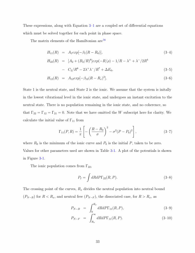
The matrix elements of the Hamiltonian are56

H11(R) = A1exp[−β1(R−R0)], (3–4)

H22(R) = [A2 + (B2/R)8]exp(−R/ρ)− 1/R− λ+ + λ−/2R4

− C2/R6 − 2λ+λ−/R7 + ∆E0, (3–5)

H12(R) = A12exp[−β12(R−Rx)2]. (3–6)

State 1 is the neutral state, and State 2 is the ionic. We assume that the system is initally

in the lowest vibrational level in the ionic state, and undergoes an instant excitation to the

neutral state. There is no population remaining in the ionic state, and no coherence, so

that Γ22 = Γ12 = Γ21 = 0. Note that we have omitted the W subscript here for clarity. We

calculate the initial value of Γ11 from

Γ11(P,R) =1

π

[−

(R−R0

σ

)2

− σ2(P − P0)2

], (3–7)

where R0 is the minimum of the ionic curve and P0 is the initial P , taken to be zero.

Values for other parameters used are shown in Table 3-1. A plot of the potentials is shown

in Figure 3-1.

The ionic population comes from Γ22,

PI =

∫dRdPΓ22(R,P ). (3–8)

The crossing point of the curves, Rx divides the neutral population into neutral bound

(PN−B) for R < Rx, and neutral free (PN−F ), the dissociated case, for R > Rx, as

PN−B =

∫ Rx

0

dRdPΓ11(R,P ), (3–9)

PN−F =

∫ ∞

Rx

dRdPΓ11(R,P ). (3–10)

33

3.3 Effect of Initial Conditions

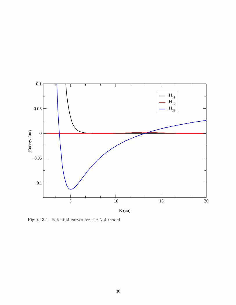
In the previous work, the initial phase space was a uniform grid, shown in Figure 3-5.

Here, we choose an orbit for the initial phase space, shown in Figure 3-6. These points

evolve in time according to Equations 3–2 and 3–3.

The results for the populations are shown in Figure 3-2. The populations of the

neutral bound and ionic states are qualitatively similar, with the orbit method showing

sharper oscillations. The population of the neutral free (dissociated) state are very similar.

If we were only concerned with the yield of the photoinduced dissociation, it would not

matter which initial conditions we chose.

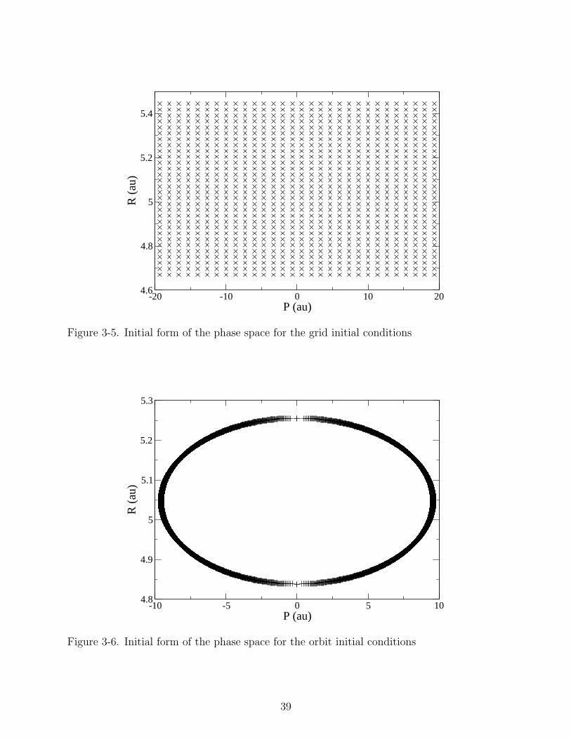
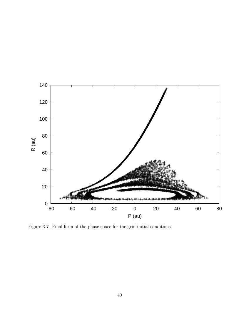
Figures 3-3 and 3-4 show the real and imaginary parts of the quantum coherence for

both the orbit and grid initial conditions. The grid method shows a larger coherence at

early times, but the two methods do not give very different results. Figures 3-7 and 3-8

show the final conformation of the phase space for the grid and orbit initial conditions.

The swirling nature of the phase space is similar to the phase space of classical particles

in a harmonic well, like the ionic potential. The free motion, which is evident in the phase

space of the grid initial conditions, does not appear here. In Figures 3-9 and 3-10 we show

the average P and R, as well as their dispersions for orbit and grid initial conditions, along

with full quantum results.

34

Table 3-1. Parameters for the NaI model.

Parameter Value (au)

R0 5.047λ+ 2.756P0 0.0λ− 43.442σ 0.12462ρ 0.660A1 0.02988∆E0 0.07626A2 101.43β1 2.158A12 0.00202β12 0.194B2 3.000Rx 13.24C2 18.950M 35,482

V . Engel and H. Metiu, J. Chem. Phys. 90, 6116 (1989)

35

5 10 15 20

R (au)

−0.1

−0.05

0

0.05

0.1

Ene

rgy

(au)

H11

H12

H22

Figure 3-1. Potential curves for the NaI model

36

0 20000 40000 60000 80000 100000 120000

t (au)

0

0.2

0.4

0.6

0.8

1

Popu

latio

n

Neutral BoundNeutral FreeNeutral Bound (grid)

Neutral Free (grid)IonicIonic (grid)

Figure 3-2. Populations for the orbit and grid initial conditions

37

0 20000 40000 60000 80000 100000 120000

t (au)

0

0.1

0.2

0.3

Coh

eren

ce

real part (grid)real part (orbit)

Figure 3-3. Real part of the coherence for the orbit and grid initial conditions

0 20000 40000 60000 80000 100000 120000

t (au)

0

0.05

0.1

0.15

0.2

Coh

eren

ce

imaginary (grid)imaginary (orbit)

Figure 3-4. Imaginary part of the coherence for the orbit and grid initial conditions

38

-20 -10 0 10 20P (au)

4.6

4.8

5

5.2

5.4

R (

au)

Figure 3-5. Initial form of the phase space for the grid initial conditions

-10 -5 0 5 10P (au)

4.8

4.9

5

5.1

5.2

5.3

R (

au)

Figure 3-6. Initial form of the phase space for the orbit initial conditions

39

0

20

40

60

80

100

120

140

-80 -60 -40 -20 0 20 40 60 80

R (

au)

P (au)

Figure 3-7. Final form of the phase space for the grid initial conditions

40

-60 -40 -20 0 20 40 60P (au)

0

10

20

30

40

50

R (

au)

Figure 3-8. Final form of the phase space for the orbit initial conditions

41

0 20000 40000 60000 80000 100000 120000

t (au)

-20

0

20

40

P

average P (orbit)average P (quantum)sigma P (orbit)sigma P (quantum)average P (grid)sigma P (grid)

Figure 3-9. Average P and σP for orbit and grid initial conditions, along with fullquantum results.

42

0 20000 40000 60000 80000 100000 120000

t (au)

0

10

20

30

<R

>

average R (orbit)

sigma R (orbit)

average R (grid)

sigma R (grid)

average R (quantum)

sigma R (quantum)

Figure 3-10. Average R and σR for orbit and grid initial conditions, along with fullquantum results.

43

CHAPTER 4NUMERICAL METHOD

4.1 A Runge-Kutta Method for Integro-Differential Equations

We begin with a general differential equation

y′(t) = f(t, y(t)). (4–1)

or, equivalently, the integrated form

y(t) = y(t0) +

∫ t

t0

f(t′, y(t′))dt′. (4–2)

A Runge Kutta method for this equation from tn to tn+1 has the following form58

k1 = f(tn, y(tn)),

k2 = f(tn + c2h, y(tn) + ha21k1),

k3 = f(tn + c3h, y(tn) + h(a31k1 + a32k2)),

... (4–3)

km = f(tn + cmh, y(tn) + h(am1k1 + . . .+ ham,m−1km−1)),

y(tn+1) = y(tn) + h(b1k1 + b2k2 + . . .+ bmkm), (4–4)

where m (an integer) is the number of stages of the method required to achieve a desired

accuracy, and the aij, bi, and ci are real coefficients. For an example set of coefficients, see

Table 4-4. The ci satisfy the relation

ci =m∑

j=1

aij. (4–5)

We can express the ki in a more compact form,

ki = f

[tn + cih, y(tn) + h

m∑j=1

aijkj

], (4–6)

44

with the constraint

aij = 0, j ≥ i, (4–7)

so that c1 = 0. We can also write the expression for y(tn+1) as

y(tn+1) = y(tn) + h

m∑i=1

biki +O(hp+1), (4–8)

where p is the order of the method. The conditions for a Runge-Kutta method to be

of order p will be discussed later. We can consider the second argument of ki as an

approximation to y(tn + cih),59 which we will call Y n

i

Y ni = y(tn) + h

m∑j=1

aijkj, (4–9)

which means

ki = f(tn + cih, Yni ), (4–10)

and the final expression for Y ni is

Y ni = y(tn) + h

m∑j=1

aijf(tn + cjh, Ynj ). (4–11)

This leads us to

y(tn+1) = y(tn) + h

m∑i=1

bif(tn + cih, Yni ) +O(hp+1). (4–12)

4.1.1 Volterra Integral Equations

Before we apply Runge-Kutta techniques to our integro-differential problem, we first

consider the integral case. A Volterra integral equation of the second kind has the form

y(t) = g(t) +

∫ t

t0

K(t, t′, y(t′))dt′. (4–13)

Here we will restrict the discussion to the linear case

y(t) = g(t) +

∫ t

t0

K(t, t′)y(t′)dt′. (4–14)

45

If we wish to propagate this equation from tn to tn+1, it is broken into two parts,36 as

y(tn+1) = qn(tn+1) + rn(tn+1), (4–15)

qn(t) = g(t) +

∫ tn

t0

K(t, t′)y(t′)dt′, (4–16)

rn(t) =

∫ t

tn

K(t, t′)y(t′)dt′ (4–17)

=

∫ t

tn

K(t, t′) [rn(t′) + qn(t′)] dt′. (4–18)

Note that qn, called the lag term, only depends on known values of y(t) (those up to

y(tn)), while rn, called the increment function, satisfies an integral equation, or an

equivalent differential equation.

If we apply the foregoing Runge-Kutta method to the expression for r, we obtain

rn(tn+1) = rn(tn) + h

m∑i=1

biK(tn+1, tn + cih) [Rni + qn(tn + cih)] , (4–19)

Rni = rn(tn) + h

m∑j=1

aijK(tn + cih, tn + cjh)[Rn

j + qn(tn + cjh)]. (4–20)

The first term, rn(tn), is zero. If we now choose the Y ni according to

Y ni = Rn

i + qn(tn + cih), (4–21)

we have

rn(tn+1) = h

m∑i=1

biK(tn+1, tn + cih)Yni , (4–22)

Y ni = qn(tn + cih) + h

m∑j=1

aijK(tn + cih, tn + cjh)Ynj . (4–23)

We can rewrite q as

qn(t) = g(t) +n−1∑

l=0

∫ tl+1

tl

K(t, t′)y(t′)dt′. (4–24)

If we apply the Runge-Kutta method for integral equations, we obtain

qn(t) = g(t) + h

n−1∑

l=0

m∑j=1

bjK(t, tl + cjh)Ylj . (4–25)

46

We can now calculate y(tn+1), according to

y(tn+1) = qn(tn+1) + rn(tn+1). (4–26)

4.1.2 Volterra Integro-Differential Equations

We now focus on the problem of the integro-differential equation

dρ(t)

dt= H(t)ρ(t) +

∫ t

t0

K(t, t′)ρ(t′)dt′, (4–27)

which is a first order Volterra integro-differential equation. To begin, we define

z(t) =

∫ t

t0

K(t, t′)ρ(t′)dt′, (4–28)

this gives

dρ(t)

dt= H(t)ρ(t) + z(t). (4–29)

The integrated form is then

ρ(t) = ρ(t0) +

∫ t

t0

(H(t′)ρ(t′) + z(t′)) dt′. (4–30)

If we also define

y(t) =

ρ(t)

z(t)

, (4–31)

M(t, t′) =

H(t) 1

K(t, t′) 0

, (4–32)

we will have an equation similar to Equation 4–30,

y(t) = y(t0) +

∫ t

t0

M(t, τ)y(τ)dτ. (4–33)

This equation is the same form as the Volterra integral equation considered earlier, with

the exception that we are now dealing with matrices.

47

The matrix y(t) contains both ρ(t) and z(t), which have integral equations that must

be solved simultaneously. If we apply the method given above, we obtain

Yni = qn(tn + cih) + h

m∑j=1

aijM(tn + cih, tn + cjh)Ynj , (4–34)

rn(t) = h

m∑i=1

biM(t, tn + cih)Yni , (4–35)

qn(t) = y(t0) + h

n−i∑

l=0

m∑j=1

bjM(t, tl + cjh)Ylj, (4–36)

y(tn+1) = rn(tn+1) + qn(tn+1). (4–37)

If we make the definitions

Yni =

P ni

Zni

, (4–38)

rn(t) =

r(ρ)n (t)

r(z)n (t)

, (4–39)

qn(t) =

q(ρ)n (t)

q(z)n (t)

, (4–40)

we have

r(ρ)n (t) =

m∑i=1

bi[H(tn + cih)Pni + Zn

i ], (4–41)

r(z)n (t) =

m∑i=1

biK(t, tn + cih)Pni , (4–42)

q(ρ)n (t) = ρ(t0) + h

n−1∑

l=0

m∑j=1

bj[H(tn + cjh)Plj + Z l

j], (4–43)

q(z)n (t) = z(t0) + h

n−1∑

l=0

m∑j=1

bjK(t, tn + cjh)Plj , (4–44)

48

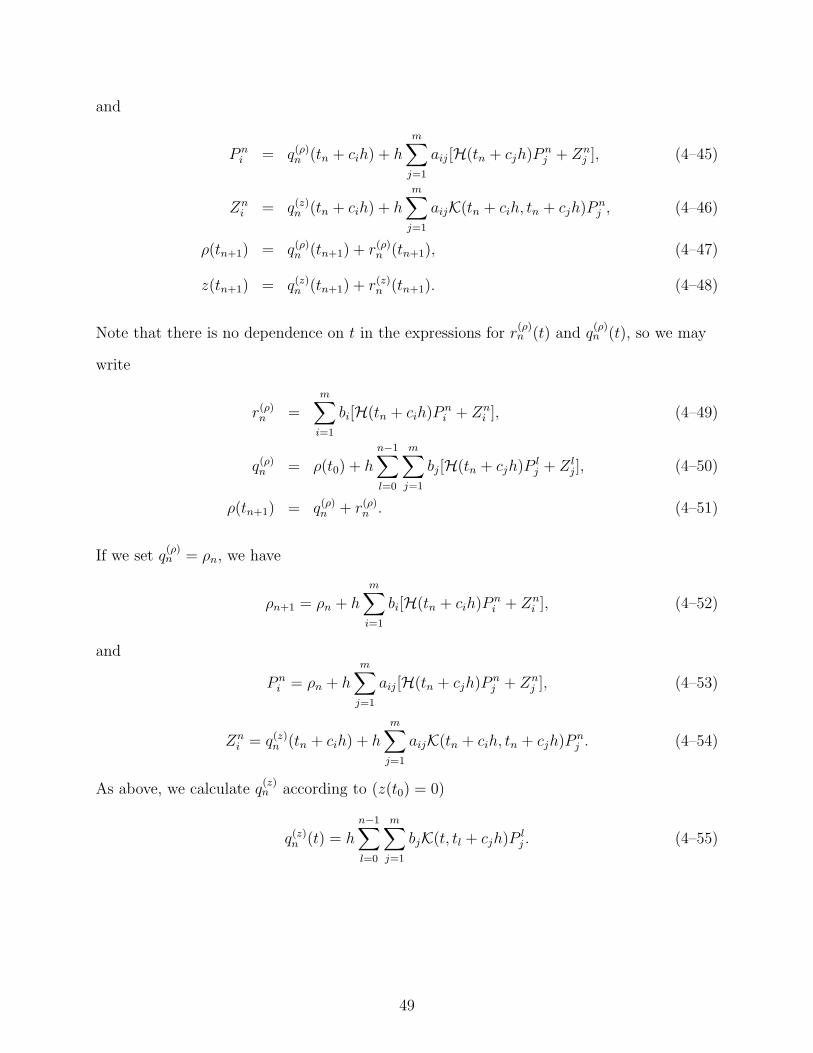
and

P ni = q(ρ)

n (tn + cih) + hm∑

j=1

aij[H(tn + cjh)Pnj + Zn

j ], (4–45)

Zni = q(z)

n (tn + cih) + h

m∑j=1

aijK(tn + cih, tn + cjh)Pnj , (4–46)

ρ(tn+1) = q(ρ)n (tn+1) + r(ρ)

n (tn+1), (4–47)

z(tn+1) = q(z)n (tn+1) + r(z)

n (tn+1). (4–48)

Note that there is no dependence on t in the expressions for r(ρ)n (t) and q

(ρ)n (t), so we may

write

r(ρ)n =

m∑i=1

bi[H(tn + cih)Pni + Zn

i ], (4–49)

q(ρ)n = ρ(t0) + h

n−1∑

l=0

m∑j=1

bj[H(tn + cjh)Plj + Z l

j], (4–50)

ρ(tn+1) = q(ρ)n + r(ρ)

n . (4–51)

If we set q(ρ)n = ρn, we have

ρn+1 = ρn + h

m∑i=1

bi[H(tn + cih)Pni + Zn

i ], (4–52)

and

P ni = ρn + h

m∑j=1

aij[H(tn + cjh)Pnj + Zn

j ], (4–53)

Zni = q(z)

n (tn + cih) + h

m∑j=1

aijK(tn + cih, tn + cjh)Pnj . (4–54)

As above, we calculate q(z)n according to (z(t0) = 0)

q(z)n (t) = h

n−1∑

l=0

m∑j=1

bjK(t, tl + cjh)Plj . (4–55)

49

4.1.3 Order Conditions

Here we will derive some of the formulas which determine the constraints on the

aij,bj, and cj for a given order p. We begin again with the simple differential equation

y′(t) = f(t, y(t)). (4–56)

If our method agrees with the Taylor series of the true solution up to the terms including

hp, then our method is of order p. The Taylor expansion of this expression, up to second

order, at t = t0 + h, is

y(t0 + h) = y(t0) + hy′(t0) + h2y′′(t0)2

+O(h3). (4–57)

We now consider the Taylor series of the approximate solution at t1 = h ,

y1(h) = y1(t0) + hy′1(t0) + h2y′′1(t0)

2+O(h3). (4–58)

The derivatives of the true solution at t0 are

y′(t)|t=t0 = f(t0, y(t0)), (4–59)

y′′(t)|t=t0 =df(t0, y(t0))

dt+ f(t0, y(t0))

df(t0, y(t0))

dy; (4–60)

and for the approximate solution

dy1

dh=

m∑i=1

biY0i + h

m∑i=1

bidY 0

i

dh, (4–61)

d2y1

dh2= 2

m∑i=1

bidY 0

i

dh+ h

m∑i=1

bid2Y 0

i

dh2. (4–62)

We now set h = 0 and note that

Y 0i |h=0 = f(t0, y0), (4–63)

dY 0i

dh|h=0 = ci

df(t0, y0)

dh+ cif(t0, y0)

df(t0, y0)

dy, (4–64)

50

which leads to

y1(t0)|h=0 = y0, (4–65)

dy1

dh|h=0 =

m∑i=1

bif(t0, y0), (4–66)

d2y1

dh2 h=0= 2

m∑i=1

bici

[df(t0, y0))

dh+ f(t0, y0)

df(t0, y0)

dy

]. (4–67)

Note that y0 = y(t0). For the two Taylor series to agree to first order in h (p = 1), the first

derivatives must agree, and we have

m∑j=1

bj = 1. (4–68)

For second order in h (p = 2), we must equate the second derivatives, and obtain

m∑j=1

bjcj =1

2. (4–69)

This method can be repeated for higher derivatives. Up to order p = 4, we have

p = 3,m∑

j=1

bjc2j =

1

3, (4–70)

m∑j=1

m∑

k=1

bjajkck =1

6, (4–71)

51

and

p = 4,m∑

j=1

bjc3j =

1

6, (4–72)

m∑j=1

m∑

k=1

bjajkcjck =1

8, (4–73)

m∑j=1

m∑

k=1

bjajkc2j =

1

12, (4–74)

m∑j=1

m∑

k=1

m∑

k=1

bjajkaklcl =1

24. (4–75)

In Table 4-1 we see the total number of equalities to be satisfied, Np, for a given order p.

For a given m, there are (m2 +m)/2 coefficients. At m = 5 it is not possible to attain

a method of order p = m = 5; there are 17 order conditions, but only 15 coefficients. In

Tables 4-2 and 4-3 we see the attainable order of a Runge-Kutta method for a given m,

and the minimum m need to obtain order p.

In Table 4-4 we see an example set of coefficients for a Runge-Kutta method with

m = p = 4.

4.2 Implicit Formulation

The previous method is an explicit formulation. However, for some cases it may be

necessary to use an implicit method.

If we adopt the diadic form, we can cast the integro-differential equation as

y′(t) = V (t)y(t) +

∫ t

0

M(t, t′)y(t′)dt′, (4–76)

52

where the dimensions of y are n2 × 1, and V and M are both n2 × n2. For a two-step

method, we can now define

Aj = hnaj1V (tn,j) + h2naj1M(tn,j, tn + dj1hn)λ1(dj1)

+ h2naj2M(tn,j, tn + dj2hn)λ1(dj2), (4–77)

Bj = hnaj2V (tn,j) + h2naj1M(tn,j, tn + dj1hn)λ2(dj1)

+ h2naj2M(tn,j, tn + dj2hn)λ2(dj2), (4–78)

Cj = Φn,j + yn[V (tn,j) + hnaj1M(tn,jtn + dj,1hn)

+ hnaj2M(tn,jtn + dj,2hn)], (4–79)

which leads to

Yn,1 = A1Yn,1 +B1Yn,2 + C1, (4–80)

Yn,2 = A2Yn,1 +B2Yn,2 + C2, (4–81)

where the dimensions of C are n2 × 1, and A and B are both n2 × n2.

4.3 Test System

To test our numerical procedure, we turn to a solved system,60,61 which is a two-state

system coupled to a bath of harmonic oscillators. The hamiltonian is

H(t) = −1

2[∆(t)σx + ε(t)σz + ζ(t)σz], (4–82)

where ∆ is an energy transfer matrix element, ε(t) is the biasing energy which may include

a driving field, and ζ(t) is a stochastic factor which contains system-bath coupling. The

σx,z are Pauli matrices. The expectation values of these matrices, 〈σi〉t, are defined as

〈σi〉t = Tr[ρ(t)σi]. These expectation values give the population difference,

〈σz〉t = ρ11 − ρ22, (4–83)

53

the real part of the coherence

1

2〈σx〉t =

1

2(ρ12 + ρ21), (4–84)

and the imaginary part

1

2〈σy〉t =

i

2(ρ12 − ρ21). (4–85)

Using these expectation values, and the fact that ρ11 + ρ22 = 1, we can express the

density matrix as

ρ(t) =1

2

1 + 〈σz〉t 〈σx〉t − i〈σy〉t〈σx〉t + i〈σy〉t 1− 〈σz〉t

. (4–86)

To account for the system bath coupling, we start with a bath at a constant

temperature T , so that

〈ζ(t)〉T = 0, (4–87)

and

〈ζ(t)ζ(0)〉T =1

π

∫ ∞

0

J(ω)cosh( ω

2T− iωt)

sinh ω2T

dω, (4–88)

where J(ω) is the spectral density of the bath, in this case taken to have an ohmic density,

as

J(ω) = 2παωe−ω/ωc . (4–89)

Here α is a dimensionless coupling parameter, and ωc is the cutoff frequency.

The time evolution of the expectation value of the Pauli matrices is governed by a set

of coupled equations,60,61

d

dt〈σz〉t =

∫ t

0

dt′[Ka(t, t′)−Ks(t, t

′)〈σz〉t′ ], (4–90)

〈σx〉t =

∫ t

0

dt′[Ys(t, t′) + Ya(t, t

′)〈σz〉t′ ], (4–91)

〈σy〉t = − 1

∆(t)

d

dt〈σz〉t, (4–92)

54

where Ks(a) and Ys(a) are symmetric (antisymmetric) memory kernels. These kernels are

Ks(t, t′) = ∆(t)∆(t′)e−Q′(t−t′) cos[Q′′(t− t′)] cos[Θ(t, t′)], (4–93)

Ys(t, t′) = ∆(t′)e−Q′(t−t′) sin[Q′′(t− t′)] cos[Θ(t, t′)], (4–94)

with

Q′(τ) = 2α ln[(ωc/πT ) sinh(πTτ)], (4–95)

Q′′(τ) = παsgn(τ), (4–96)

Θ(t, t′) =

∫ t

t′ε(τ)dτ, (4–97)

where T is the temperature of the reservoir. The antisymmetric kernels, Ka and Ya, are

similar to the symmetric ones, except with every sine replaced by a cosine, and cosines

replaced by sines. It should be noted that these kernels use the noninteracting-blip

approximation (NIBA).62 In the case of high temperatures, the approximation

Q′(τ) = 2α ln(ωc/πT ) + 2απT |τ | (4–98)

can be used. in this approximation, the equations can be solved exactly.

The equations for 〈σx〉t and 〈σz〉t are the ones chosen to test the computational

method. Note that while the expression for 〈σz〉t is an integro-differential equation, 〈σx〉t is

governed by an integral equation. Our method should work in either case.

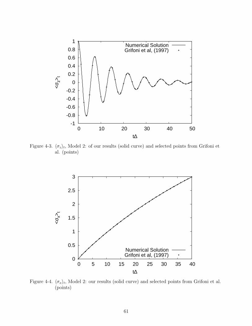
We calculate 〈σx〉t and 〈σz〉t for two models; in Model 1 α = 0.1, T = 0.5∆, ε =

−0.5∆, ωc = 30∆, and in Model 2 α = 0.05, T = 0.05∆, ε = 0, ωc = 30∆. For convenience,

we have set ∆ = 1. Model 1 is a high temperature case for which the markovian limit

may be applicable. Model 2 is a lower temperature, unbiased case. The initial state is

one in which the population is in the state 1, with no coherence, so that 〈σz〉0 = 1, and

〈σx〉0 = 〈σy〉0 = 0.

In Figures 4-1 and 4-2 we compare results using the Runge-Kutta method with those

found in a previous study60 for Model 1. Results for Model 2 are presented in Figures 4-3

55

and 4-4. There is very good agreement in all cases. As a further test, we calculate 〈σz〉t in

the high temperature limit, where exact results are available, presented in Figures 4-5 and

4-5. At short times the results agree very well, but there are some small deviations at long

times. These deviations are small enough to consider our method to be a reliable one.

Finally, we calculate 〈σz〉t for Model 1 in two approximations - the instantaneous

dissipation limit, and the markovian limit. In the instantaneous dissipation limit, we

assume the kernels are rapidly changing relative to 〈σz〉. We then assume 〈σz〉t′ = 〈σz〉t so

that

d

dt〈σz〉ID

t =

∫ t

0

dt′Ka(t, t′)− 〈σz〉ID

t

∫ t

0

dt′Ks(t, t′). (4–99)

In the Markoff limit, we assume the integral in 4–99 can be extended to infinity, giving

d

dt〈σz〉ID

t =

∫ ∞

0

dt′Ka(t, t′)− 〈σz〉ID

t

∫ ∞

0

dt′Ks(t, t′). (4–100)

The results are shown in Figure 4-7. All three methods give the same value at long

(equilibrium) times, however neither method fully describes the short time dynamics.

The Markoff limit yields an exponential decay, while in the instantaneous case there are

oscillations that are damped compared to the delayed dissipation case.

4.4 Scaling and Limitations

The majority of the computer processing time in this method is devoted to calculating

the q(z)n term, which grows more expensive as more steps are taken. The methods scales in

processing time as (number of steps)2. As we are dealing with matrices, it also scales as

(number of states)2. However, q(z)n requires quantities that have already been calculated -

values from previous steps. It is easy to divide q(z)n into chunks which do not depend on

each other, so this process can be split among several processors. The program has been

designed with this feature, and scales linearly with the number of processors allotted; e.g.

it will run twice as fast if twice as many processors are allotted. We have used both the

OpenMP standard,63 as well as the MPI standard.64 It should be noted that either one

56

standard or the other is used, not both. The program must be compiled with different

options for each standard.

The memory required for the program to run may also become an issue as larger and

longer runs are considered. As written, the numerical method requires the storage of all of

the previous values of the density matrix, along with the intermediate values within each

time step (m of them at each step).

4.5 The Memory Time

By default, the memory term involves all previous states, back to the beginning of

the simulation. As more steps are taken, the process becomes more expensive. It may,

however, be possible to reduce the running time with the concept of a memory time

(tmem). In this case, correlations longer then tmem are neglected. This means setting

z(t) =

∫ t

t−tmem

K(t, t′)ρ(t′)dt′ (4–101)

for t > tmem. For a fixed step size, tstep, the method scales as (tmem/tstep)2, but will scale

linearly with t once t > tmem.

The option of using a memory time will depend on the system being studied. The

memory time depends on the kernel, K(t, t′); it will be the cutoff time after which the

kernel is negligible,

K(t, t′) ≈ 0,

t− t′ > tmem. (4–102)

In the case of Equation 2–30, the memory time will depend on the correlation function,

C(t). If the correlation function is small enough to be neglected after tmem, then the entire

kernel will be small enough to be neglected, since each term is multiplied by C(t). The

57

dissipative part of the master equation is then

(d

dtρab

)

diss

= −∑

cd

∫ t

tmem

dt′[Mcd,db(−(t− t′))eiωda(t−t′)ρac(t′) +Mac,cd(t− t′)eiωbc(t−t′)ρdb(t

′)

− Mdb,ac(−(t− t′))eiωbc(t−t′)ρcd(t′)−Mdb,ac(t− t′)eiωda(t−t′)ρcd(t

′)]. (4–103)

Note that the minimum value of t′ is t − tmem, which means that we can discard any

previous values of ρ(t′) where t′ < t − tmem, potentially reducing computational memory

overhead.

The idea of a memory time also leads to a different way of treating the initial state

of a system. Often the initial state of a system is assumed to be in thermal equilibrium

at a specified temperature. It is then natural to assume that the system will remain in

that state in the absence of any external driving force. However, the memory kernel at

early times in general will not vanish, leading to changes in the populations. Beginning

the simulation has the effect of switching on the correlations between the primary region

and the medium. One approach to dealing with this is to run the simulation without

any external driving forces until the system returns to equilibrium and then apply any

nonequilibrium influences, such as a light pulse.

Using the memory time allows for a different approach. We consider the system to

be in thermal equilibrium, and to have been in that equilibrium for the duration of tmem.

This means setting

ρ(−tmem < t < 0) = ρ(0) = ρeq, (4–104)

where ρeq is the equilibrium density matrix. Doing so allows us to account for correlations

occuring before the beginning of the simulation, without actually calculating any dynamics

for those previous times. Returning to Equation 2–28, at t = 0 we will have

∂ρ(0)

∂t= − i

~

[H ′, ρ(0)

]+

∫ 0

−tmem

K(t, t′)ρ(t′)dt′, (4–105)

58

and at the first step in the simulation, t1 ,

∂ρ(t1)

∂t= − i

~

[H ′, ρ(t1)

]+

∫ t1

t1−tmem

K(t, t′)ρ(t′)dt′. (4–106)

Negative values of ρ are handled according to Equation 4–104. If we choose our memory

time properly, there should be no inital dynamics - the system will be in a true equilibrium.

4.6 Conclusion

In this chapter we have developed a method for solving integro-differential equations

based on the Runge-Kutta algorithm. The order of the method depends on the number

of steps in each iteration, along with a set of constants chosen. The order requirements,

along with the conditions that the constants must fulfill, have been discussed.

We then tested this method on a solved example found in the literature, using a

fourth-order four step explicit method. Our method gives excellent agreement, for both

integral and integro-differential equations. This method can be used with matrices, so it is

applicable to the second-order equation of motion for the reduced density matrix.

Table 4-1. Number of equalities to be satisfied for a given order of the Runge-Kuttamethod

p 1 2 3 4 5 6 7 8 9 10Np 1 2 4 8 17 37 85 200 486 1205

Table 4-2. Highest attainable order of an explicit Runge-Kutta method for a given m

m 1 2 3 4 5 6 7 8 9 10p 1 2 3 4 4 5 6 6 7 7

Table 4-3. Minimum m needed to attain a given order p

p 1 2 3 4 5 6 7 8 9 10m 1 2 3 4 6 7 9 11 12 13

59

-0.6

-0.4

-0.2

0

0.2

0.4

0.6

0.8

1

0 5 10 15 20 25 30

<σ z

>t

t∆

Numerical SolutionGrifoni et al, (1997)

Figure 4-1. 〈σz〉t, Model 1: our results (solid curve) and selected points from Grifoni et al.(points)

-0.1

0

0.1

0.2

0.3

0.4

0.5

0.6

0 5 10 15 20 25 30

<σ x

>t

t∆

Numerical SolutionGrifoni et al, (1997)

Figure 4-2. 〈σx〉t, Model 1: our results (solid curve) and selected points from Grifoni et al.(points)

60

-1

-0.8

-0.6

-0.4

-0.2

0

0.2

0.4

0.6

0.8

1

0 10 20 30 40 50

<σ z

>t

t∆

Numerical SolutionGrifoni et al, (1997)

Figure 4-3. 〈σz〉t, Model 2: of our results (solid curve) and selected points from Grifoni etal. (points)

0

0.5

1

1.5

2

2.5

3

0 5 10 15 20 25 30 35 40

<σ x

>t

t∆

Numerical SolutionGrifoni et al, (1997)

Figure 4-4. 〈σx〉t, Model 2: our results (solid curve) and selected points from Grifoni et al.(points)

61

-0.6

-0.4

-0.2

0

0.2

0.4

0.6

0.8

1

0 10 20 30 40 50

<σ z

>t

t∆

Exact SolutionNumerical Solution

Figure 4-5. 〈σz〉t, Model 1: the high temperature limit. Exact results (solid curve) andcalculated results (dashed curve)

-1

-0.5

0

0.5

1

0 10 20 30 40 50

<σ z

>t

t∆

Exact SolutionNumerical Solution

Figure 4-6. 〈σz〉t, Model 2: the high temperature limit. Exact results (solid curve) andcalculated results (dashed curve)

62

Table 4-4. Example coefficients

c A = aij0 0 0 0 012

12

0 0 012

0 12

0 01 0 0 1 0bT 1

613

13

16

-0.6

-0.4

-0.2

0

0.2

0.4

0.6

0.8

1

0 10 20 30 40 50

<σ z

>t

t∆

Delayed DissipationInstantaneous Dissipation

Markoff Limit

Figure 4-7. 〈σz〉t, Model 1 : delayed dissipation (solid curve), instantaneous dissipation(dashed curve), and the Markoff limit (dotted curve)

63

CHAPTER 5VIBRATIONAL RELAXATION OF ADSORBATES ON METAL SURFACES

5.1 Introduction

We now have a general numerical method for integro-differential equations, which can

be used to study dissipative dynamics of molecular systems. In this chapter, we consider

the vibrational relaxation of adsorbates on metal surfaces - specifically CO/Cu(001),

CO/Pt(111), and Na/Cu(001). Previous work on these systems8,15,18 considered only

electronic dissipation. Here we focus on vibrational dissipation.

We consider the frustrated translation of the adsorbate, and examine the effects of

different coupling strengths and temperatures. We also demonstrate the instantaneous and

markovian limits. We consider only the ground and first excited vibrational state, which

leads to relatively simple expressions for the populations and coherences. In later chapters,

we will study the complex dynamics which arises from adding more states.

5.2 Model Details

Here we are concerned with the frustrated translation (T-mode) of an adsorbate

on a metal surface. The T-modes are low energy vibrations, and are populated at the

temperatures studied. The specific systems studied are CO/Cu(001), CO/Pt(111),

and Na/Cu(001) which have been the subject of much experimental and theoretical

work.29,37,65–68 We consider the frustrated T-mode (the P or primary region) as a

harmonic oscillator coupled to a bath of harmonic oscillators69 (the R or reservoir)

with the Hamiltonian

H = HP + HR + HPR, (5–1)

HP = ~ω0a†a, (5–2)

HR =∑

j

~ωj b†j bj, (5–3)

HPR = ~∑

j

κj(a†b†j + a†bj + ab†j + abj), (5–4)

64

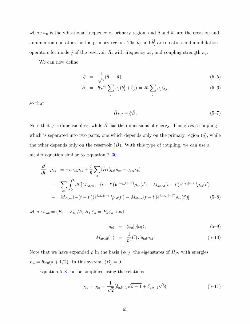
where ω0 is the vibrational frequency of primary region, and a and a† are the creation and

annihilation operators for the primary region. The bj and b†j are creation and annihilation

operators for mode j of the reservoir R, with frequency ωj, and coupling strength κj.

We can now define

q =1√2(a† + a), (5–5)

B = ~√

2∑

j

κj(b†j + bj) = 2~

∑j

κjQj, (5–6)

so that

HPR = qB. (5–7)

Note that q is dimensionless, while B has the dimensions of energy. This gives a coupling

which is separated into two parts, one which depends only on the primary region (q), while

the other depends only on the reservoir (B). With this type of coupling, we can use a

master equation similar to Equation 2–30

∂

∂tρab = −iωabρab +

i

~∑

c

〈B〉(qcbρac − qacρcb)

−∑

cd

∫ t

0

dt′[Mcd,db(−(t− t′))eiωda(t−t′)ρac(t′) +Mac,cd(t− t′)eiωbc(t−t′)ρdb(t

′)

− Mdb,ac(−(t− t′))eiωbc(t−t′)ρcd(t′)−Mdb,ac(t− t′)eiωda(t−t′)ρcd(t

′)], (5–8)

where ωab = (Ea − Eb)/~, HPφa = Eaφa, and

qab = 〈φa|q|φb〉, (5–9)

Mab,cd(τ) =1

~2C(τ)qabqcd. (5–10)

Note that we have expanded ρ in the basis φa, the eigenstates of HP , with energies

Ea = ~ω0(a+ 1/2). In this system, 〈B〉 = 0.

Equation 5–8 can be simplified using the relations

qab = qba =1√2(δa,b+1

√b+ 1 + δa,b−1

√b), (5–11)

65

and

qaa = 0. (5–12)

If we consider only the ground (0) and first excited state (1), we have, after some

rearrangement, and setting ~ = 1,

d

dtρ00 = −1

2

∫ t

0

[4 cos(ω0(t− t′))ReC(t− t′)ρ00(t′)

−(C(−(t− t′))e−iω0(t−t′) + C(t− t′)eiω0(t−t′)

)]dt′, (5–13)

d

dtρ11 = −1

2

∫ t

0

[4 cos(ω0(t− t′))ReC(t− t′)ρ11(t′)

−(C(−(t− t′))eiω0(t−t′) + C(t− t′)e−iω0(t−t′

)]dt′, (5–14)

d

dtρ01 = iω0ρ01 − i

∫ t

0

2ReC(t− t′)Imρ01(t′)dt′, (5–15)

d

dtρ10 = −iω0ρ10 − i

∫ t

0

2ReC(t− t′)Imρ10(t′)dt′. (5–16)

For a two-state case, with this choice of qab, there is no coupling between the states. This

is because we are dealing with only a 2×2 matrix, and we can simplify the equations using

the relations ρ00 + ρ11 = 1 and ρ01 = ρ∗10, where the ∗ superscript indicates the complex

conjugate. However, as we will see in later chapters, for three or more states, couplings do

appear.

If we assume the instantaneous dissipation limit, we can take ρ outside of the integral,

and for the ground state population we have

d

dtρ

(ID)00 = −1

2ρ

(ID)00

∫ t

0

4 cos(ω0(t− t′))ReC(t− t′)dt′

−∫ t

0

(C(−(t− t′))e−iω0(t−t′) + C(t− t′)eiω0(t−t′)

)dt′, (5–17)

which is an integral equation. Extending the integral to infinity gives the markoff limit,

d

dtρ

(ID)00 = −1

2ρ

(ID)00

∫ ∞

0

4 cos(ω0(t− t′))ReC(t− t′)dt′

−∫ ∞

0

(C(−(t− t′))e−iω0(t−t′) + C(t− t′)eiω0(t−t′)

)dt′. (5–18)

66

5.3 The Correlation Function

We yet need the time correlation function C(t), which can be obtained from the

spectral function J(ω) from40

C(t) =

∫ ∞

0

[cos(ωt) coth

(~ω

2kBT

)− i sin(ωt)

]ω2J(ω)dω. (5–19)

The spectral function can be derived from the spectral density, g(ω), and the coupling

strength, κ(ω), through ω2J(ω) = 2g(ω)|κ(ω)|2. We use a Debye model, so that

g(ω) = 18πNω2/ω3D, (5–20)

where ωD is the Debye phonon cutoff frequency, so g(ω) = 0 for ω > ωD, and N is the

number of lattice atoms. For the couplings, we follow38 and use

|κ(ω)|2 = [p+ q(ω − ω0)]/N, (5–21)

which gives

J(ω) = 36π[p+ q(ω − ω0)]/ω3D, (5–22)

where p and q are parameters which depend on the system. The values of these and other

parameters used in the calculations are given in Table 5-1.

The imaginary part of the correlation function, which is temperature independent,

can be integrated exactly. For t = 0, the real part can be integrated exactly as well.

For t 6= 0, however, this is not the case. For large enough temperatures, we can use the

approximation

coth

(~ω

2kBT

)≈ 2kBT

~ω+

~ω6kBT

. (5–23)

This leads to an expression that can be integrated exactly. This approximation has been

tested, and shown to give excellent agreement down to temperatures as low as 100K.

The correlation functions that arise from these parameters are shown in Figure 5-1 for

temperatures of 150K, 300K, and 450K.

67

Increasing the temperature increases the magnitude of the real part of the correlation

function, but has no effect on the frequency of the oscillations. This frequecy is about

9.6 × 10−4 au−1, which is close to the Debye frequency. The correlation function is largest

at short times, showing a 1/t type decay at long times.

5.4 Results

For each system, we have the initial conditions of the population entirely in the

excited state with no coherence, so that ρ11 = 1, ρ00 = 0, and ρ01 = ρ10 = 0. We

then follow the relaxation towards thermal equilibrium, for temperatures of 150K and

300K. The results are shown in Figures 5-2, 5-3, and 5-4. In each case, we see large initial

oscillations, which relax towards equilibium within 30,000 to 50,000 au. Increasing the

temperature seems to damp the oscillations, with relaxation to equilibrium coming sooner.

This increase is in qualtitative agreement with experiment.67

We have also repeated the runs for CO/Cu(001)with different coupling strengths, to

test the effect on the relaxation. In Figure 5-5 we see the effect of reducing the coupling

to 80% of normal, while in Figure 5-6 the coupling has increased to 120%. The coupling

is linear in p and q, so multiplying each by 0.8 has the effect of decreasing it to 80% of

normal. To increase to 120%, we multiply by 1.2. Decreasing the coupling means weaker

interactions with the reservoir, leading to more oscillations and an increase in relaxation

time. Increasing the coupling has the reverse effect. In each case, the final equilibrium

values are the same.

We have also tested the applicability of the instantaneous and markovian limits.

Results for CO/Cu(001) at 150K are shown in Figure 5-7. The instantaneous dissipation

limit shows very strong oscillations, even surpassing 1 (full population). This shows

that instantaneous dissipation does not work in this case. That is to be expected, as the

correlation function does not decay rapidly enough. The markovian limit shows a very fast

exponential rise to the equilibrium value. The markovian limit thus gives correct values at

68

long times, but cannot capture the short time dynamics like the full delayed dissipation

treatment can.

Finally, we present results for the quantum coherences for CO/Cu(001) in Figures 5-8

and 5-9. The coherences are not coupled to the populations, so if they are zero initially,

then they will remain zero. For these runs, the initial conditions are ρ01 = 0.1 + 0.1i.

Both the real and imaginary parts of the coherence decay over longer periods of time than

the populations, showing oscillations on the order of ω0, gradually going to zero. At short

times, the imaginary part has a similar pattern to the populations.

Our initial conditions are that the population begins entirely in the excited state,

with no coherence. This would be achieved by a very rapid transition from the ground

state to the excited state. In fact, experimental studies have shown that there is a very

fast excitation, followed by a slow relaxation.22 The relaxation time from experiment for

CO/Cu(001) at 150K is a few picoseconds.22,67 Our calculations show relaxation in about

one picosecond (1 ps = 41,300 au), which is a good qualitative agreement. In addition,

experiments have shown a decrease in the relaxation time at higher temperatures, which

is the trend seen here. Only the delayed dissipation treatment gives this good agreement.

The relaxation shown in the markovian limit is much too rapid.

5.5 Conclusions

We have studied the dissipative dynamics of a two state system coupled to a reservoir,

however the method laid out in this chapter can be used in systems with more states.

Here we have calculated the reduced density matrix for the evolution of the frustrated

T-mode vibration of an adsorbate on a metal surface. The system began in the excited

state, and the relaxation over time was calculated. Our calculated relaxation times are in

good agreement with experiment.

We have repeated the calculations using the markovian and instantaneous dissipation

limits. Each limit gives the correct results at long times, but the short time dynamics

69

are only properly described by the delayed dissipation method. The instantaneous limit

appears to be invalid in this case, giving results that exceed 1 (100% population).

There are two trends shown in the results. Increasing the temperature decreases

the oscillations, and leads to a faster relaxation to equilibrium. Increasing the coupling

strength has a similar effect. The markovian limit, which shows no oscillations and a very

fast relaxation, will be the most useful in high temperature/large coupling situations.

However, when these criteria are not met, or when detailed short time dynamics are

important, the delayed dissipation treatment is required.

Table 5-1. Frequencies and coupling parameters

Na/Cu CO/Cu CO/Ptω0 2.205× 10−4au−1 1.448× 10−4au−1 2.183× 10−4au−1

ωD 1.013× 10−3au−1 1.013× 10−3au−1 7.283× 10−4au−1

p 2.31× 10−7au−2 6.44× 10−8au−2 1.10× 10−8au−2

q −5.80× 10−5au−1 1.58× 10−5au−1 3.98× 10−6au−1

J . L. Vega, R. Guantes, S. Miret-Artes, and D. A. Micha, J. Chem. Phys. 121, 8580 (2004)

70

0 50000 100000

t (au)

−5e−06

0

5e−06

Im C

(t)

0 20000 40000

t (au)

−2e−05

0

2e−05R

eal C

(t)

150K300K450K

Figure 5-1. Upper: Real part of C(t) for CO/Cu(001) at 150K, 300K, and 450K. Lower:Imaginary part of C(t) for CO/Cu(001) at 150K

71

0 20000 40000

t (au)

−0.5

0

0.5

1

ρ 00

ρ00 , (150Κ, upper)ρ00− 0.6, (300K, lower)

Figure 5-2. Population of the ground state (ρ00) for CO/Cu(001) at 150K and 300K

72

0 10000 20000 30000

t

−0.5

0

0.5

1

ρ 00 ρ00 , (150K, upper)ρ00 − 0.6, (300K, lower)

Figure 5-3. Population of the ground state (ρ00) for Na/Cu(001) at 150K and 300K

73

0 50000 100000

t

−0.5

0

0.5

1

ρ 00

ρ00 , (150K, upper)ρ00 − 0.6, (300K, lower)

Figure 5-4. Population of the ground state (ρ00) for CO/Pt(111) at 150K and 300K

74

0 20000 40000

t (au)

−0.5

0

0.5

1

ρ 00

ρ00 , (1.0x coupling, upper)ρ00 − 0.6, (0.8x coupling, lower)

Figure 5-5. Population of the ground state (ρ00) for CO/Cu(001) at 150K for normalcoupling strength and at 0.8 times the coupling strength

75

0 20000 40000

t (au)

−0.5

0

0.5

1

ρ 00

ρ00 , (1.0x coupling, upper)ρ00 − 0.6, (1.2x coupling, lower)

Figure 5-6. Population of the ground state (ρ00) for CO/Cu(001) at 150K for normalcoupling strength and at 1.2 times the coupling strength

76

0 20000 40000 60000t (au)

0

0.5

1

ρ 00

Instantaneous DissipationDelayed DissipationMarkovian Dissipation

Figure 5-7. Population of the ground state (ρ00) for CO/Cu(001) at 150K using delayeddissipation, the instantaneous dissipation limit , and the Markoff limit

77

0 1000000 2000000 3000000

t (au)

−0.1

−0.05

0

0.05

0.1

Rea

l(ρ01

)

150K300K

Figure 5-8. Real part of the quantum coherence ρ01 for CO/Cu(001) at 150K (solid line)and 300K (dashed line)

78

1000000 2000000

t (au)

−0.02

−0.01

0

0.01

0.02

Im(ρ

01)

150K300K

0 20000 40000 60000t (au)

−0.2

−0.1

0

0.1

Im(ρ

01)

Im(ρ01

), (150K, upper)Im(ρ

01) − 0.1, (300K, lower)

Figure 5-9. Imaginary part of the quantum coherence ρ01 at short times for CO/Cu(001)at 150K and 300K (upper) and long times (lower)

79

CHAPTER 6ELECTRONIC AND VIBRATIONAL RELAXATION

6.1 Introduction

In the previous chapter, we studied the dissipative dynamics of adsorbates on metal

surfaces, considering only two vibrational states in a single electronic state. For that

model considered, there are no couplings between states. In this chapter, we explore what

happens when more vibrational states are considered, which does lead to couplings. We

also consider two electronic states, which adds electronic dissipation to our equations,

allowing for electronic relaxation. This also allows us to add a laser pulse to cause

excitation from the ground state to an excited electronic state. Here we will consider only

the system CO/Cu(001). Previous work on this system7,8,39 has included only electronic

dissipation; here we consider vibrational dissipation as well.

6.2 Model Details

Adding a light pulse to the system requires consideration of the interaction between

the pulse (L) with the primary region and with the reservoir. We now have the hamiltonian

H(t) = H0 + HPL(t) + HRL(t), (6–1)

where H0 was our hamiltonian in the absence of a pulse, and HPL and HRL are the

interaction of the regions with light, which in the dipole approximation are

HPL(t) = −DPEP (t), (6–2)

HRL(t) = −∫d3rEext(t)PR, (6–3)

where DP is the electric dipole of the primary region and PR is the dipole per unit volume

in the reservoir. The external field is described by Eext, and EP is the local value inside the

primary region.

To describe the electronic states, we divide the system into a primary region which

includes the adsorbate and adjacent metal atoms, and the reservoir, which includes the

80

rest of the system39 as shown in Figure 6-2. This model has been used previously for

studies of photodesorption. Here, we will restrict the distance from the surface to the

adsorbate, Z, to its equilibrium value in the ground excited state, Zg. The angles θ and φ

are set to zero.

6.3 Primary Region

The parameters for the primary region come from a ZINDO parameterization.70,71

This is a semiempirical method, which is applicable to transition metals. There are two

versions of ZINDO: ZINDO/1 is used for calculating ground state properties, such as bond

distances, and ZINDO/S is used for calculating excited electronic state properties.72 Six

copper atoms were included, and ZINDO/1 calculations were carried out for the ground

electronic state. The results were then rescaled to fit available experimental results for the

equilibrium distance from the surface to the adsorbate, as well as the binding energy.73–76

The electronic excited state was parameterized using ZINDO/S calculations, along with

the transition dipole between the electronic states.

The ground and excited state potentials are7

Vg(Z, x, θ, φ) = V 0g (θ)e

−2αg(θ)h√

x2+(Z−γdCO)2−Zg(θ)+γdCO

i

− 2V 0g (θ)e

−αg(θ)h√

x2+(Z−γdCO)2−Zg(θ)+γdCO

i+

1

2MCOΩg(Z)2x2, (6–4)

Ve(Z, x, θ, φ) = ∆Ve + V 0e (θ)e

−2αe(θ)h√

x2+(Z−γdCO)2−Ze(θ)+γdCO

i

− 2V 0e (θ)e

−αe(θ)h√

x2+(Z−γdCO)2−Ze(θ)+γdCO

i+

1

2MCOΩe(Z)2x2, (6–5)

where V 0g,e(θ) are potential well depths, αg,e(θ) are the widths of the wells, γ = MO/(MC +

MO, with MO,MC , and MCO are the masses of oxygen, carbon, and carbon monoxide. The

C-O bond distance is dCO, here taken to be constant; Zg,e(θ) is the equilibrium distance

from the center of mass of CO to the copper surface. The frequency of the frustrated

translation is ωg,e. The potentials were found to be only weakly dependent on φ, and its

contribution here has been neglected.

81

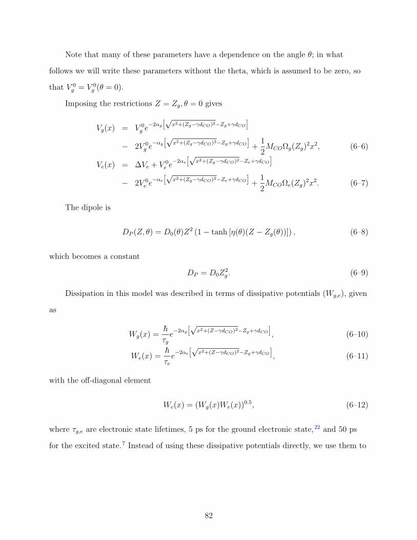
Note that many of these parameters have a dependence on the angle θ; in what

follows we will write these parameters without the theta, which is assumed to be zero, so

that V 0g = V 0

g (θ = 0).

Imposing the restrictions Z = Zg, θ = 0 gives

Vg(x) = V 0g e−2αg

h√x2+(Zg−γdCO)2−Zg+γdCO

i

− 2V 0g e−αg

h√x2+(Zg−γdCO)2−Zg+γdCO

i+

1

2MCOΩg(Zg)

2x2, (6–6)

Ve(x) = ∆Ve + V 0e e−2αe

h√x2+(Zg−γdCO)2−Ze+γdCO

i

− 2V 0e e−αe

h√x2+(Zg−γdCO)2−Ze+γdCO

i+

1

2MCOΩe(Zg)

2x2. (6–7)

The dipole is

DP (Z, θ) = D0(θ)Z2 (1− tanh [η(θ)(Z − Zg(θ))]) , (6–8)

which becomes a constant

DP = D0Z2g . (6–9)

Dissipation in this model was described in terms of dissipative potentials (Wg,e), given

as

Wg(x) =~τge−2αg

h√x2+(Z−γdCO)2−Zg+γdCO

i, (6–10)

We(x) =~τee−2αe

h√x2+(Z−γdCO)2−Zg+γdCO

i, (6–11)

with the off-diagonal element

Wc(x) = (Wg(x)We(x))0.5, (6–12)

where τg,e are electronic state lifetimes, 5 ps for the ground electronic state,22 and 50 ps

for the excited state.7 Instead of using these dissipative potentials directly, we use them to

82

build Lindblad operators41,42 for the electronic dissipation

(∂ρ

∂t

)el

diss

= − 1

2~([W,ρ(t)]+ − 2W 0.5ρ(t)W 0.5

). (6–13)

Values of the constants used are shown in Table 6-1. The electronic dissipation is done

with the Lindblad operators, while the vibrational dissipation is done using the delayed

dissipation treatment outlined in Chapter 5.

These potentials are functions of x and must be expanded in a harmonic oscillator

basis set φi(x) to include the vibrational states. The potentials for the ground and excited

state are cast in matrix form, as

V =

Vg Vc

Vc Ve

, (6–14)

where

(Vg)ij =

∫dxφ∗i (x)Vg(x)φj(x), (6–15)

with s similar expression for Ve. The coupling between the states depends on the dipole,

and the secondary region, discussed later. The Lindblad matrices are

W =

Wg Wc

Wc We

, (6–16)

with

(Wg)ij =

∫dxφ∗i (x)Wg(x)φj(x), (6–17)

and similar expressions for We and Wc. The equation for the density matrix is then

dρ(t)

dt= − i

~[V, ρ(t)]− 1

2~([W, ρ(t)]+ − 2W0.5ρ(t)W0.5

)−∫ t

0

K(t, t′)ρ(t′)dt′ (6–18)

where K(t, t′) is a supermatrix containing all of the elements from Equation 5–8.

83

6.4 Secondary Region

The secondary region contains the rest of the copper surface. Here we make a two

band approximation, leading to a 2 × 2 density matrix. To distinguish it from the density

matrix of the primary region, we will call the secondary region density matrix γ. The two

states here are the conduction band (c) and the unoccupied band (u), and we consider

only vertical transitions between the two levels.39 We cast the density matrix in terms of

the Pauli matrices,

γ(t) =1

2I +

3∑i

γiσi, (6–19)

with

γ1 = Re(γcu), (6–20)

γ2 = −Im(γcu), (6–21)

γ3 =1

2(γcc − γuu). (6–22)

These components evolve in time according to the optical Bloch equations2,8,77

∂γ1

∂t= ω2f(t)γ3 − γ1

τcoh

, (6–23)

∂γ2

∂t= −ω1f(t)γ3 − γ1

τcoh

, (6–24)

∂γ3

∂t= (ω1γ2 − ω2γ1)− γ3 − γ3

τpop

, (6–25)

where τcoh is the coherence time, τpop is the population difference decay time, and γ3 is the

long time equilibrium value of γ3. These terms are related to the excitation rate, κ+, the

deexcitation rate, κ−, and the decoherence rate, κ0, according to

τcoh = 2(κ+ + κ− + κ0)−1, (6–26)

τpop = (κ+ + κ−)−1, (6–27)

γ3 =τpop

2(κ− − κ+). (6–28)

84

The Ω are given by

Ω1 = −2

~Re(d(el)

cu E0), (6–29)

Ω2 =2

~Im(d(el)

cu E0), (6–30)

where d(el)cu is the electronic dipole between the bands. The f(t) term is the laser field

envelope, chosen here to be

f(t) = e−4(t−t0)/τ2p cos(ω0t), (6–31)

where t0 is the center of the pulse, τp is the width, and ω0 is the frequency. The excitation

and deexcitation rates can be calculated from the state to state energy transfer rate, Rtr

as

κ+ = guRtr, (6–32)

κ− = gcRtr, (6–33)

where gc,u are the density of states of bands c and u. Values of the parameters used on the

optical Bloch equations are given in Table 6-2.

The value of the electric field inside the primary region depends on properties of the

secondary region, and is given by

EP = −2N∗el(t)d(el)cu γ2

|zs − zp|3 , (6–34)

where N∗el is excited electron density in the metal, given by

N∗el = N0 +N∗(t), (6–35)

where N0 is the number of electrons always available for excitation and N∗(t) is the

number of inflowing electrons. This evolves over time according to

dN∗(t)dt

= S(t)BsN0 −Kd(t)N∗(t), (6–36)

85

where Bs is a parameter related to the size of the S region, S(t) is a source term, and Kd

is the rate at which hot electrons decay to the deexcited gas state. This rate is calculated

from

Kd =gep

γelTel(t), (6–37)

where gep is the electron-phonon coupling constant, Tel is the electronic temperature, and

the elecronic specific heat is Cel = γelTel. The electronic temperature and the lattice

temperature, Tlat, are calculated from the heat diffusion equations22,78

dTel

dt=

gep(Tlat − Tel) + S(t)

γelTel

, (6–38)

dTlat

dt=

gep(Tlat − Tel)

Clat

, (6–39)

where Clat is the specific heat of the lattice. Parameters for the heat diffusion equations

are given in Table 6-3.

6.5 Unperturbed Dynamics

We first consider the system with no external pulse. The initial state is a Boltzmann

thermal distribution. In Figure 6-3 we have the results showing the population of the

ground electronic ground vibrational state, along with the coherence between the ground

vibrational state and the second excited vibrational state. After 20,000 au, the system

settles into a repeating beat pattern. The oscillations are large, and the effects of adding

a light pulse would be difficult to determine. This behavior is dictated by the correlation

function, which describes the coupling of the medium to the system. In this case, the

correlation function is large, indicating a strong coupling. This accounts for the large

oscillations. In addition, the correlation function does not decay rapidly; it falls off as

time−1. This may be the cause of the long-lived oscillations.

6.6 Results With a Pulse

To account for the oscillations that occur in the unperturbed case, we run our

calculations twice. The first is the unperturbed case, which gives an idea of how long

86

it takes the system to settle into a repeating pattern. Once that time is known, we run

the calculations again, adding the light pulse only after the system has settled. We then

subtract the unperturbed population, ρ0(t), from the populations with the pulse to get the

change,

∆ρ(t) = ρ(t)− ρ0(t) (6–40)

which shows the overall effect of the pulse.

The pulse is similar to that used in the previous chapter, a gaussian of width 100

fs, fluence of 3.0 mJ/cm2, and frequency 620 nm. In figure 6-4 we see the population

differences. The pulse causes an excitation to the excited state, which decays to the

ground state. The overall shape of the decay is due to the electronic dissipation. There is

a beat pattern of oscillations in the populations; this is due to the vibrational dissipation.

The coherences show this beat pattern as well, decaying to zero as the populations return

to equilibrium. This same beat pattern is seen in the unperturbed dynamics.

6.7 Conclusion

When the correlation function is large and long lived, the system may not settle into

a stable thermal equilibrium state. Long-lived oscillations in the populations need to be

accounted for, to see the effects of a pulse. In the case of CO/Cu(001), we have added a

laser pulse after a long simulation time, then subtracted the results from the no-pulse case

in order to see the effects of the pulse. The pulse populates the excited electronic state,

which then relaxes to the ground electronic state. The vibrational populations show a

beat pattern as they are populated by the pulse and then gradually are depleted by the

electronic dissipation.

87

Figure 6-1. Energy diagram for CO/Cu(001)

Cu

Cu Cu

CuCu Cu

C

O

Zx

θ

φ

Figure 6-2. CO/Cu(001), reprinted with permission from A. Santana and D. A. Micha,Chem. Phys. Lett. 369, 459 (2003)

88

Table 6-1. Parameters for the ground and excited state potentials

Parameter Value (atomic units)Vg 2.68× 10−2

Ve 4.45× 10−2

αg 1.52αe 2.02Zg 4.83Ze 5.16γ 0.572dCO 2.17MCO 5.22× 104

ωTg 1.45× 10−4

γ 0.572D0 1.12× 10−2

Table 6-2. Parameters for secondary region

Parameter Value (atomic units)dcu 0.02gc 20.0Ry−1

gu 1.0Ry−1

zs 1.0zp 4.83τpop 620.1τcoh 1157κ0 8.959× 104

Rtr 3.83× 10−5

Table 6-3. Parameters for the heat diffusion equations

Parameter Value (atomic units)gep 8.22× 10−14

γel 3.283× 10−12

Clat 1.190× 107

89

0 50000 1e+05t (au)

0

0.1

0.2

0.3

0.4

0.5

Popu

latio

n

g0real g02

Figure 6-3. Populations without a pulse of the ground electronic ground vibrational (g0)state, along with the coherence between the ground electronic groundvibrational state and the ground electronic second vibrational state (g02) at300K

90

1e+05 1.5e+05 2e+05t (au)

-0.02

0

g0

-0.02

0

Den

sity

Cha

nges

g1

-0.02

0

g2

-0.01

0real g02im g02

Figure 6-4. Population differences at 300K with a pulse, for the three vibrational states inthe ground electronic state

91

CHAPTER 7ELECTRONICALLY NON-ADIABATIC DYNAMICS OF Ag3Si(111):H

7.1 Introduction

We now turn our attention to the system of a small cluster of silver atoms on a silicon

surface, Ag3Si(111):H. Here we are interested in electronic and vibrational dissipation as

they relate to possible pathways of electron transfer induced by a laser pulse. This pulse

may cause a transition directly from the initial state to the final, electron-transferred

state. We call this direct excitation. Alternatively, the pulse may cause a transition to an

intermediate state, or perhaps a series of intermediate states, which then relax into the

electron-transferred state. This is indirect excitation.

In this chapter we consider both direct excitation and indirect excitation with one

intermediate state. For indirect excitation, we now have three electronic states, with

vibrational relaxation within each state, along with electronic couplings and relaxation

between them. The direct excitation case is a two-electronic-state case, similar to that in

the previous chapter. However, the correlation function for Ag3Si(111):H is very different,

and the differencing method used previously is not needed.

7.2 Model Details

As in the previous chapter, we will treat electronic dissipation and vibrational

dissipation separately. The general equation of motion for the density matrix is

∂ρ

∂t= − i

~[H

′, ρ] +

(∂ρ

∂t

)

el,diss

+

(∂ρ

∂t

)

vib,diss

. (7–1)

Each of the three terms is defined below. The Hamiltonian H′contains elements for each

state as well as couplings between them. For direct excitation, we expand in a basis of two

electronic states, the ground state, g, and the final excited state, e, so that

H′dir =

Hgg Hge

Heg Hee

. (7–2)

92

For indirect excitation, we have a basis of three electronic states, the ground state g, an

intermediate excited state e, and the final state f , so that

H′indir =

Hgg Hge Hgf

Heg Hee Hef

Hfg Hfe Hff

. (7–3)

The off diagonal elements are the couplings between the states, and will include the effects

of the light pulse and any other non-dissipative couplings.

Each electronic state is then expanded in a basis of harmonic oscillator states, φi,vi,

where i = g, e, f is the electronic state and vi = 0, 1, 2 . . . is the vibrational state. The

density matrix is solved in this basis of vibronic states, so that

ρI,J = 〈φI |ρ|φJ〉, (7–4)

where we use the capital letters I and J to denote a vibronic state, so that φI = φi,vi.

The g electronic state is coupled to the e and f states through the light pulse. We use

the dipole to calculate the effect of the light pulse (l) on the system,

H(l)ij = −DijE(t), (7–5)

where E(t) is the light pulse and Dij is the dipole between electronic states i and j. We

calculate the full vibronic couplings through the Franck-Condon overlap79,80

SI,J = 〈i, vi|j, vj〉, (7–6)

where SI,J is the overlap between electronic state i in vibrational state vi and electonic

state j in vibrational state vj. The coupling due to light in the full vibronic basis is then

H(l)I,J = H

(l)ij SI,J . (7–7)

The physical parameters of our model are taken from a recent ab initio density

functional study25 using periodic boundary conditions81. The model has four layers of

93

silicon; each layer is 4 × 6 atoms. The surface bonds unoccupied by the adsorbed silver

cluster are saturated by hydrogen atoms, giving a total composition of Ag3Si96H21. A

picture of the system is shown in Figure 7-1. The transition dipoles (Dij) were calculated

using Kohn-Sham orbitals generated from augmented plane-wave density functional

calculations, using fixed atomic positions82. The transition dipoles were then used to

calculate the transition oscillator strengths (fij), according to

fij =2mωij

~D2

ij. (7–8)

There are many transitions in this system. Here we choose specific transitions

according to two criteria: the transition must have a large oscillator strength and a large

change in the electronic population in the silver cluster (∆n Ag3). The parameters for the

chosen transitions are shown in Table 7-1.

The primary region is the silver cluster, along with the adjacent silicon and hydrogen

atoms. We again consider both electronic relaxation and vibrational relaxation of the

primary region.

Electronic relaxation is calculated using Lindblad dissipation41,42,

(∂ρ

∂t

)

el,diss

= −1

2[L†L, ρ]+ + LρL†, (7–9)

where [, ]+ denotes the anticommutator, and L is a matrix derived from the relaxation

rates as

LIJ = r(I → J)0.5, (7–10)

where r(I → J) is the transition rate from state I to state J . The transition rate

from the excited state (e) to the ground state (g), r(e → g), is approximated from

experiment83,84. Here we have chosen two values for the relaxation time, τeg, 200 fs and 1

ps. The transition rate is the inverse of the relaxation time, r(e→ g) = τ−1eg

94

To get the rate between different vibrational states, we use Franck-Condon factors79,80,

r(e, ve → g, vg) = r(e→ g)S2

eve,gvg∑i,j S

2evi,gvj

. (7–11)

The reverse rate is calculated by detailed balance, as

r(g, vg → e, ve) = r(e, ve → g, vg)exp (− [E(e, ve)− E(g, vg)] /2kbT ) , (7–12)

where E(e, ve) is the energy of the excited electronic state in the ve vibrational state, T is

the temperature, and kb is the Boltzmann constant. In this case, the energy differences are

so large that there are essentially no transitions from the ground state up to the excited

state via Lindblad dissipation.

Vibrational relaxation is calculated using delayed dissipation, Equation 2–30. We

assume there are no interactions via delayed dissipation across electronic states, meaning

the vibrational states in the ground electronic state are coupled to each other, but not to

the vibrational states in the excited electronic state, and vice versa.

7.3 Correlation Function

We calculate the correlation function according to Equation 5–19. The spectral

density coming from the ab initio treatment is shown in Figure 7-4. There is a single

large peak near 70 meV that dominates the spectral density. This is in the area of surface

vibrations; bulk modes do not couple strongly to the vibrations of the silver cluster.

The correlation function is shown in Figures 7-5 and 7-6. The magnitude of the

correlation function is much smaller than that for CO/Cu(001). It also has a nearly

gaussian shape, and decays exponentially. This fast decay should lead to shorter lived

oscillations.

7.4 Direct Excitation

7.4.1 Initial Dynamics

In the case of direct excitation, shown in Figure 7-2, the pulse excites the system

directly from the initial ground state to the final state. The final state chosen here has

95

a strong oscillator strength, as well as a large charge transfer. The minima of the two

potentials, qg and qe are not the same, and the overlap between the states depends on the

difference between the two, ∆q.

We first consider the system without the addition of a light pulse, to determine if

there are any initial dynamics which must be accounted for. The initial state is entirely in

the ground electronic state, with a thermal distribution of vibrational states, at 300 K. At

this temperature, the excited electronic state is not significantly populated. We consider

five vibrational states in each electronic state, for a total of ten vibronic states. The

populations of the ground state, g0, and the coherence between the ground and second

excited vibrational state, g02, are shown in Figure 7-7. When there is no pulse, the only

driving force is the delayed dissipation. In this case, the dissipation is weak, and has little

effect on the population. There is some change in the populations, shown in the upper

panel of Figure 7-7, however, the changes are not nearly as strong as in CO/Cu(001),

and a differencing method is not required. We can assume the system begins in a stable

thermal equilibrium.

7.4.2 Photoinduced Dynamics

We repeat the simulation, this time adding a pulse. The pulse parameters are the

same as those used in the previous chapters. Because the dissipation is weak, we have also

repeated the simulation including the pulse and Lindblad dissipation, but not the delayed

dissipation. The total ground and electronic populations are shown in Figures 7-8 and 7-9.

The pulse causes a large transfer of population from the ground state to the excited state,

which then decays smoothly back to the ground state. This decay is due to the Lindblad

dissipation. As the transition rate is decreased (by increasing the time from 200 fs to 1

ps), the decay takes longer. The electronic relaxation dominates the dynamics. There is

some change in the populations at early times when delayed dissipation is added, but this

effect disappears as time goes on.

96

In Figure 7-10 we focus on only the highest energy state to see the effects of delayed

dissipation. While there is some effect, the population oscillates around the case without

delayed dissipation. The other populations show a similar pattern. It may be that these

effects are important early in the dynamics, however the light pulse and the electronic

relaxation are the dominant factors. In this case, the dynamics are largely captured by

including only the electronic dissipation.

The quantum coherence between states e0 and e1 is shown in Figure 7-11. The

coherence peaks early, around 2500 au, just as the e state is being populated by the pulse.

The coherence has disappeared by 40,000 au.

7.5 Indirect Excitation

In the case of indirect excitation, depicted in Figure 7-3, the light pulse excites from

the initial ground state (g) to an excited state (e), which then relaxes into the final state

(f). This final state is the electron-transferred state. The intermediate excited state has a

large oscillator strength, but small charge transfer. The final state couples strongly to the

intermediate state, but weakly to the ground state, so there is little direct excitation. The

final state has a large charge transfer.

The strong coupling between the g and e states leads to electronic relaxation, which is

again treated with the Lindblad form. Here we have chosen to use only the 200 fs rate for

the relaxation. The coupling between the g and f states is so small that the relaxation is

very slow, and has been neglected in our calculations. The vibrational coupling is treated

with delayed dissipation, with no vibrational coupling across electronic states.

The e and f electronic states are are coupled through momentum,85,86 as

Vef = −~2

m〈e| ∂∂q|f〉 ∂

∂q, (7–13)

where m is the mass of the silver cluster. We need the coupling not just between electronic

states, but also the vibrational states, so we expand this expression in terms of harmonic

97

oscillator states to give

〈ve|Vef |vf〉 = −~2

m

∑

v′f

〈e, ve| ∂∂q|fv′f〉〈v

′f |∂

∂q|vf〉. (7–14)

In our notation |e, ve〉 is the e electronic state in the ve = 0, 1, 2 . . . vibrational state.

The first term can be expressed as a Franck-Condon overlap and a coupling factor, cef ,

which depends only on the electronic states, to give

〈ve|Vef |vf〉 = −~2

2

∑

v′f

〈e, ve|fv′f〉cef〈v′f |∂

∂q|vf〉, (7–15)

The last term can be expressed in terms of the creation and annihilation operators a† and

a as

〈v′f |∂

∂q|vf〉 = − 1

~√

2〈v′f |(a† − a)|vf〉

= − 1

~√

2(√vf + 1δv′f ,vf+1 −

√vfδv′f ,vf−1). (7–16)

Inserting this into Equation 7–15 gives

〈ve|Vef |vf〉 = cef~m

(√vf + 1

2〈e, ve|fvf+1〉 −

√vf

2〈e, ve|fvf−1〉

), (7–17)

which is the expression used to calculate the coupling. The cef term comes from the ab

inito study, and is 1.764× 10−4 au.

7.5.1 Initial Dynamics

We again test the initial equilibrium by considering the system in the absence of a

light pulse. We add five vibrational states in the f electronic state, for a total of fifteen

states. The initial state is in a thermal distribution of vibrational states in the ground

electronic state at 300 K. The intermediate electronic state is lower in energy than the

final electronic state, but is not low enough to be populated at this initial temperature.

98

The populations at 300 K without a pulse are shown in Figure 7-12. The results

are similar to the direct case, with small oscillations that rapidly decay. There is no

population in either the e or f states.

7.5.2 Photoinduced Dynamics

The pulse used here is the same as for the direct case. We assume that, as before,

there are no initial dynamics which must be accounted for. The populations are shown

in Figure 7-13, for results with and without delayed dissipation. In each case, the

Lindblad dissipation is included. While the delayed dissipation has little effect on the

total population of the intermediate state, there is a noticeable increase in the population

of the final, charge transferred state. In this case, the electronic dissipation is still the

dominant driving force, but the delayed dissipation does have an effect and should be

included. Vibrational relaxation enhances the transfer into the final state. The final

population of the charge transferred state is aout 3.5%. In this model, this population is

long-lived, and could lead to surface photovoltage.

7.5.3 Memory Time

The delayed dissipation in this model is weak, and its effects decay after a short

period of time. This model then is a good test for use of the memory time concept, as

detailed in Section 4.4. If our results with a memory time are the same as those obtained

using the full memory kernel, then we may be able to use the memory time to speed up

our simulations, and overcome some of the computational problems which can arise when

large systems or long simulation times are considered.

The memory time approach also changes our initial state. In the previous simulations

we begin with the system in a thermal distribution at t = 0. In this case, the system is

not only in a thermal distribution at time t = 0, but it has also been in that state for

the duration of tmem. This should change the dynamics for the different states in different

ways, depending on whether or not they are initially populated. For the g states, which

are all initially populated, we expect the initial oscillations to either disappear, or at

99

least be reduced. We should see a more stable initial state. For initially unpopulated

states, we should see no change in the dynamics. At the beginning of the simulation, there

should be no change; the initial population is zero, so any memory terms involving these

populations will also be zero. If we have chosen a long enough memory time, we should see

no deviations later in the simulation either, since we are only discarding very small values

of the memory kernel.

Returning to Figure 7-12, we see that most of the oscillations in the g0 population

have largely subsided by 50,000 au. We then take this value for the memory time,

tmem, and truncate the memory term as shown in Equation 4–103. We then repeat

the simulation with the same parameters as before.

In the absence of a light pulse, we expect more stable initial dynamics. The

populations of the g3 and g4 states are shown in Figure 7-14 for the full memory

kernel, and using the memory time cutoff. There are some very slight oscillations in

the populations when using the memory time, but overall it is much more stable initially

than in the full memory kernel case. The initial state of the system more closely resembles

a stationary thermal equilibrium.

When a pulse is added, the dynamics should be similar between the two approaches.

Results for the g electronic state populations are shown in Figure 7-15, along with the

previous results which include the entire memory kernel. The populations of the g states

are very similar, although there are some small differences in them. The g0 state has the

largest difference, with the memory time approach giving a smaller value at long times.

However, these differences are small, and one can consider the memory time approach

effective.

The populations of the e and f electronic states are shown in Figures 7-16 and

7-17. These states are not populated initially, so we expect to see no difference in the

populations. This is exactly what is seen - the memory time approach gives the same

results.

100

7.6 Conclusions

In the case of Ag3Si(111):H, the correlation function is small, and decays rapidly. This

leads to delayed dissipation having little effect on the dynamics. Initially, the system can

be considered to be in a stable thermal equilibrium, there is no reason to extend the initial

part of the simulation to account for any correlations.

In the case of direct excitation, when a pulse is added, there are transitions to the

excited states, then a relaxation dominated by the electronic terms. The vibrational

(delayed) dissipation plays a very small role. In the case of indirect excitation, including

the delayed dissipation does have an effect on the dynamics - there is an increase in the

final population of the final state.

We have also tested our memory time approach and achieved good results. There

are some small diferences for initially populated states, but the results for initially

unpopulated states are the same as those obtained using the full memory kernel. The

memory time approach would be very well suited for a system which has relatively few

initally populated states, with many initially unpopulated states. This approach can also

give an initial state which is close to a stable thermal equilibrium.

Table 7-1. Parameters for the chosen transitions in Ag3Si(111):H

System Transition ω, au ∆E, au fij ∆q, au ∆nAg3Si - 1.0858 × 10−3 0 0 0 0

Ag+3 Si− HOMO-4 → LUMO+3 9.9410 × 10−4 7.3965 × 10−2 0.1067 -6.4407 × 10−2 -0.2816

Ag3Si∗ HOMO → LUMO+15 9.1339 × 10−4 7.2359 × 10−2 0.6442 -3.9081 × 10−2 0.0145Ag−3 Si+ HOMO → LUMO+12 1.1270 × 10−3 6.8163 × 10−2 0.0036 -2.3497 × 10−2 0.3542

101

Figure 7-1. Ag3Si(111):H, reprinted with permission from D. S. Kilin and D. A. Micha, J.Phys. Chem. C 113, 3530 (2009)

102

Figure 7-2. Energy diagram for Ag3Si(111):H, direct excitation

Figure 7-3. Energy diagram for Ag3Si(111):H, indirect excitation

103

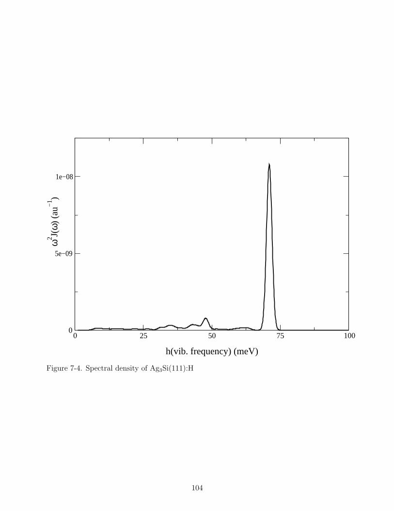
0 25 50 75 100

h(vib. frequency) (meV)

0

5e−09

1e−08

ω2 J(

ω)

(au−

1 )

Figure 7-4. Spectral density of Ag3Si(111):H

104

0 20000 40000 60000 80000

t (au)

−4e−08

−2e−08

0

2e−08

4e−08

Rea

l C(t

) (a

u−2 )

Figure 7-5. Real part of the correlation function of Ag3Si(111):H

105

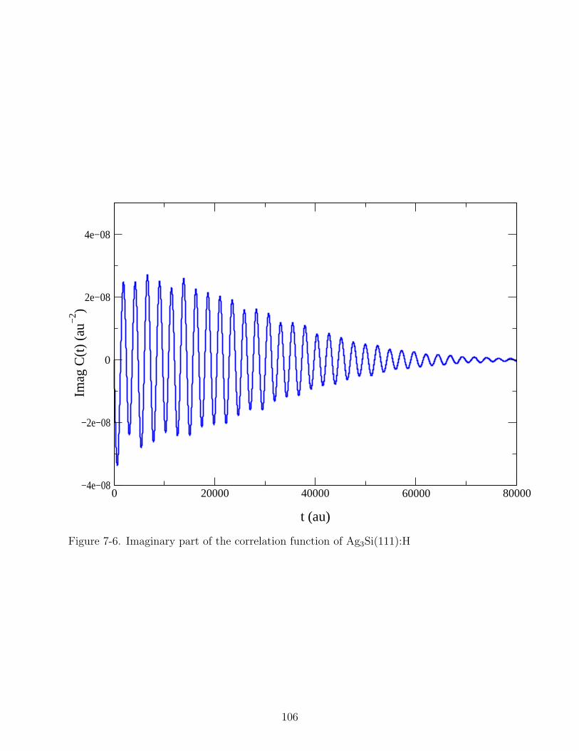
0 20000 40000 60000 80000

t (au)

−4e−08

−2e−08

0

2e−08

4e−08

Imag

C(t

) (a

u−2 )

Figure 7-6. Imaginary part of the correlation function of Ag3Si(111):H

106

0 20000 40000 60000t (au)

0

0.1

0.2

0.3

0.4

0.5

0.6

Popu

latio

n

g0g02

0.682

0.684

0.686

g0

Figure 7-7. The g0 population and g02 coherence without a pulse

107

0 20000 40000 60000t (au)

0

0.5

1

Popu

latio

n

Pg, DD

Pe, DD

Pg, no DD

Pe,no DD

Figure 7-8. Total population of the ground and excited electronic states with and withoutdelayed dissipation, τel = 200 fs

108

0 20000 40000 60000t (au)

0

0.5

1

Popu

latio

n

Pg, DD

Pe, DD

Pg,no DD

Pe, no DD

Figure 7-9. Total population of the ground and excited electronic states with and withoutdelayed dissipation, τel = 1 ps

109

0 20000 40000 60000t (au)

0

0.02

0.04

0.06

Popu

latio

n

e4, no DDe4, DD

Figure 7-10. Population of the e4 state, with and without delayed dissipation

110

0 20000 40000 60000t (au)

-0.05

0

0.05

0.1

Coh

eren

ce

real e01im e01

Figure 7-11. Quantum coherence between states e0 and e1

111

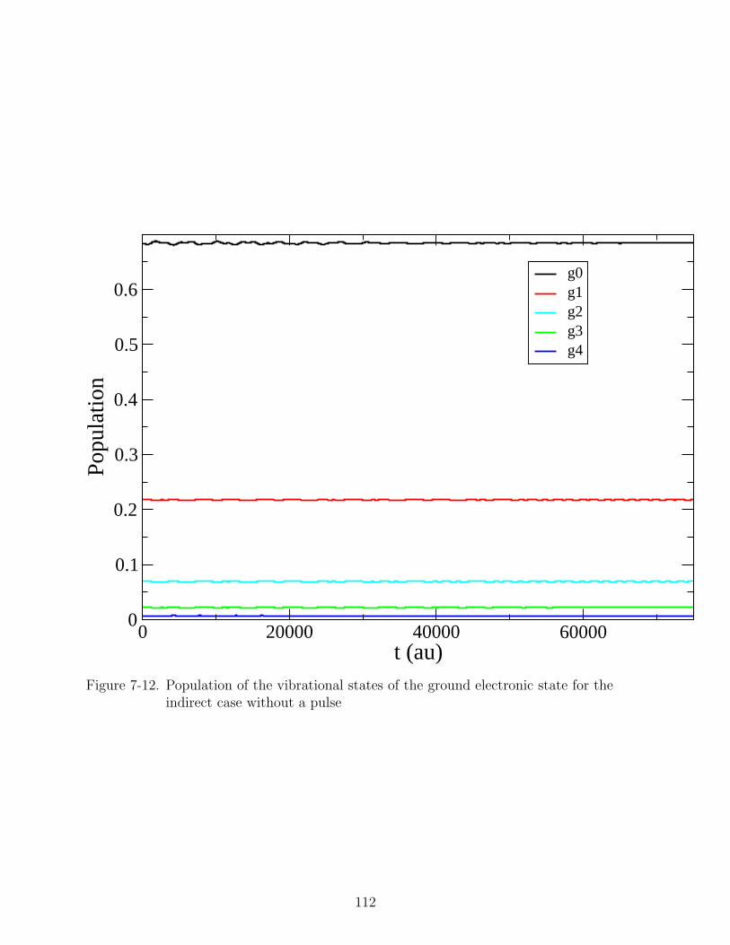
0 20000 40000 60000t (au)

0

0.1

0.2

0.3

0.4

0.5

0.6

Popu

latio

n

g0g1g2g3g4

Figure 7-12. Population of the vibrational states of the ground electronic state for theindirect case without a pulse

112

0 20000 40000 60000t (au)

0

0.2

0.4

0.6

0.8

1

Popu

latio

n

Pg, DD

Pe, DD

Pf, DD

Pg, no DD

Pe, no DD

Pf, no DD

Figure 7-13. Total population of the ground, excited, and final electronic states with andwithout delayed dissipation, τel = 200 fs

113

0 20000 40000t (au)

0

0.01

0.02

Popu

latio

n

g3g4g3, t

mem

g4, tmem

Figure 7-14. Populations of the g3 and g4 states without a light pulse, using either the fullmemory kernel or the memory time

114

0 20000 40000 60000t (au)

0

0.1

0.2

0.3

0.4

0.5

0.6

Popu

latio

n

g0g1g2g3g4

Figure 7-15. Vibrational populations of the ground electronic state with the full memory(dashed curve) and using a memory time of 50000 au (solid curve)

115

0 20000 40000 60000t (au)

0

0.05

0.1

0.15

0.2

0.25

Popu

latio

n

e0e1e2e3e4

Figure 7-16. Vibrational populations of the excited electronic state, e, with the fullmemory (dashed curve) and using a memory time of 50000 au (solid curve)

116

0 20000 40000 60000t (au)

0

0.005

0.01

0.015

0.02

Popu

latio

n

f0f1f2f3f4

Figure 7-17. Vibrational populations of the final electronic state, f , with the full memory(dashed curve) and using a memory time of 50000 au (solid curve)

117

CHAPTER 8CONCLUSION

In this work, we have laid out the theoretical framework for studying different forms

of energy dissipation in quantum-mechanical systems. We have also developed a numerical

method for propagating the integro-differential equations which come out of the theory.

We have also shown how this approach may be extended to quantum-classical systems.

We have tested our method on physical systems which include dissipation due to

both vibrational and electronic relaxation. Our method also allows for the excitation

of the system by a light pulse. These systems have both fast dissipation, and slow

(delayed) dissipation. We have seen that the correlation function, which describes the

coupling between the primary region and the reservoir, determines the effect of the delayed

dissipation.

In the case of adsorbates on metal surfaces, our calculated relaxation times agree

well with available experimental results. We have also studied two mechanisms of electron

transfer induced by a light pulse in a metal cluster on a semiconductor surface. Both

direct and indirect excitation can lead to charge transfer; the indirect excitation case

produces a long lived charge transfer state.

8.1 Vibrational Relaxation

Initially, we focused on only vibrational relaxation. We have shown, in the case

of a strong coupling to the medium, only the full delayed dissipation treatment can

fully describe the dynamics. The instantaneous and markovian limits do give correct

equilibrium values, but do not capture the short-time dynamics.

The delayed dissipation may have such a strong effect that there are oscillations at

the beginning of the simulation, before any pulse is added. When this is the case, we have

used a differencing method to determine the effects of an added pulse. This effect occurs

when the correlation function is large and long-lived. When the correlation function is

118

small and decays rapidly, these inital effects do not appear, and no differencing method is

required.

8.2 Electronic and Vibrational Relaxation

Our method is capable of handling different types of dissipation at the same time.

We have used a Lindblad formalism to treat electronic dissipation, while treating the

vibrational dissipation with a memory kernel. In the systems studied, we have seen that

the electronic relaxation tends to dominate the overall dynamics. Including the vibrational

relaxation is necessary to obtain the correct long-time results, and to see fine structure in

the short-time dynamics.

8.3 Program Development

Our program has been applied to studies of dissipation in quantum mechanical

systems, but it is not limited to these. It has been designed to solve integral and

integro-differential equations of a general form. In addition, it has been designed to run on

systems with parallel processors; we have used both the OpenMP and MPI standards to

give the program the widest use on different systems.

The core of the program, which handles the numerical algorithms, is very general, and

is kept separate from the modules which handle system-specific functions. This allows for

the program to be applied easily to many different systems, with a minimum of recoding.

8.4 Future Work

We have focused on small systems - no more than fifteen states. However, our

program is general enough to handle larger systems. Adding more states adds computer

time, but this effect can be mitigated somewhat by allowing additional processors to run

the code. We can also implement the idea of a memory time, where correlations that occur

before a specified time are ignored. This allows the method to scale better, and allow

for more states to be considered. Doing so could allow for more complex systems to be

studied.

119

We have also shown how dissipation could be handled in a quantum-classical

treatment. The programs which handle dissipation and the quantum-classical treatment

are separate; however it should be possible to combine them into one program capable of

dealing with dissipation in both quantum and quantum-classical systems.

120

APPENDIX APROGRAM DETAILS

A.1 Overview

Our program is designed to solve matrix-valued integro-differential equations,

using Runge-Kutta integration schemes. It has been applied to Liouville-von Neumann

equations, but its use is not limited to these. There are two types of equations considered.

The first, which is the more general, is

∂ρ(t)

∂t= f [t, ρ(t), z(t)] (A–1)

with

z(t) =

∫ t

0

K [t, t′, ρ(t′)] dt′ (A–2)

This must be solved using an explicit method. There is also the linear case, where

∂ρ(t)

∂t= V (t)ρ(t) +

∫ t

0

M(t, t′)ρ(t′)dt′ (A–3)

This special case of the first equation can be solved using either an explicit or implicit

method.

There are two separate modules of the program. The first, StoreAll.f90, contains

the Runge-Kutta propagation code. This module is independent of the system being

solved, and should not be altered. The second module, funcs.f90, contains the

model-specific details. This section handles the calculation of f and z, and also controls

the output format. The program is written completely in Fortran 90.

A.2 Model Specific Functions

The file funcs.f90 contains the following functions and subroutines, all of which are

required by the program.

• init funcs This subroutine handles any operations that must happen in the

beginning of the simulation. These may include reading parameters, initializing

variables, or opening required input or output files.

121

• final funcs This subroutine is called at the end of the simulation. Possible

operations performed here are recording end values or averages, and closing files.

• rho0 This subroutine sets the inital value of the density matrix, ρ(0).

• do f This subroutine calculates f as in equation A–1, where t, ρ(t) and z(t) are

assumed to be given.

• do V This subroutine calculates V as in equation A–3. This subroutine is only called

when implicit integration is used.

• do k This subroutine calculates K as in equation A–1, where t, t′, and ρ(t′) are

assumed to be given.

• do M This subroutine calculates M as in equation A–3. This subroutine is only called

when implicit integration is used.

• write rho This subroutine is called at the end of each propagation step. It controls

the output. In the simplest case, it can record the current t and ρ(t) to an output

file. However, it could be used for more detailed output if desired. The output files

needed should be opened during init funcs, and closed in final funcs.

A.3 Input And Output Files

The program uses the following input files:

• PVDRK.in - this file contains all of the constants required. These include those

relevant to the model system, as well as calculation parameters (stepsize, etc.). The

constants are enumerated in a simple variable = value format.

• mX.in - Here ’X’ is the order of the integration, for a fourth-order calculation,

the program will open m4.in. This file contains the parameters for the a, b, and c

matrices in the Runge-Kutta algorithm. This is only required currently for explicit

methods. For implicit methods currently only one fourth-order method is supported,

and the constants for it are stored in the program itself.

• Others - it may be required to add additional input files to be read by the system

module, funcs.f90. For example, in the case of Ag3Si(111):H we have also used

122

nElec.in, which specifies the number of electronic and vibrational states as well as

parameters for each state.

123

REFERENCES

[1] U. Fano, Rev. Modern Phys. 29, 74 (1957).

[2] K. Blum, Density Matrix Theory and Applications, Plenum, New York, 1996.

[3] J. A. Prybyla, T. F. Heinz, J. A. Misewich, M. M. T. Loy, and J. H. Glownia, Phys.Rev. Lett. 64, 1537 (1990).

[4] J. A. Prybyla, H. W. K. Tom, and G. D. Aumiller, Phys. Rev. Lett. 68, 503 (1992).

[5] L. Cai, X. D. Xiao, and M. M. T. Loy, Surf. Sci. 464, L727 (2000).

[6] L. Cai, X. D. Xiao, and M. M. T. Loy, J. Chem. Phys. 115, 9490 (2001).

[7] Z. Yi, D. A. Micha, and J. Sund, J. Chem. Phys. 110, 10562 (1999).

[8] D. A. Micha, A. Santana, and A. Salam, J. Chem. Phys. 116, 5173 (2002).

[9] C. Springer, M. Head-Gordon, and J. C. Tully, Surf. Sci. 320, L57 (1994).

[10] C. Springer and M. Head-Gordon, Chem. Phys. 205, 73 (1996).

[11] P. Saalfrank, R. Baer, and R. Kosloff, Chem. Phys. Lett. 230, 463 (1994).

[12] P. Saalfrank and R. Kosloff, J. Chem. Phys. 105, 2441 (1996).

[13] P. Saalfrank, Chem. Phys. 211, 265 (1996).

[14] O. Kuhn and V. May, Chem. Phys. 208, 117 (1996).

[15] Z. G. Yi, D. Beksic, and D. A. Micha, Intern. J. Quantum Chem. 64, 71 (1997).

[16] D. A. Micha and Z. G. Yi, J. Chem. Soc., Faraday Trans. 93, 969 (1997).

[17] D. A. Micha and Z. G. Yi, Chem. Phys. Lett. 298, 250 (1998).

[18] D. A. Micha and A. Santana, J. Phys. Chem. A 105, 2468 (2001).

[19] D. A. Micha, J. Phys. Chem. 107, 7311 (2003).

[20] A. Santana and D. A. Micha, Chem. Phys. Lett. 369, 459 (2003).

[21] A. Leathers and D. A. Micha, J. Phys. Chem. A 110, 749 (2006).

[22] T. A. Germer, J. C. Stephenson, E. J. Heilweil, and R. R. Cavanagh, J. Chem. Phys.101, 1704 (1994).

[23] J. C. Owrutsky, J. P. Culver, and M. Li, J. Chem. Phys. 97, 4421 (1992).

[24] T. A. Germer, J. C. Stephenson, E. J. Heilweil, and R. R. Cavanagh, J. Chem. Phys.98, 9986 (1993).

124

[25] D. S. Kilin and D. A. Micha, J. Phys. Chem. C 113, 3530 (2009).

[26] D. S. Kilin and D. A. Micha, Chem. Phys. Lett. 461, 266 (2008).

[27] R. C. Tolman, The Principles of Statistical Mechanics, Clarendon Press, Oxford,England, 1938.

[28] J. von Neumann, Mathematical Foundations of Quantum Mechanics, Princeton Univ.Press, Princeton, New Jersey, 1955.

[29] F. Hofmann and J. P. Toennies, Chem. Rev. 96, 1307 (1996).

[30] C. Meier and D. J. Tannor, J. Chem. Phys. 111, 3365 (1999).

[31] T. Mancal and V. May, Eur. Phys. J. B. 18, 633 (2000).

[32] T. Mancal and V. May, J. Chem. Phys. 114, 1510 (2001).

[33] N. Makri, J. Phys. Chem. A 102, 4414 (1998).

[34] J. Stockburger and C. H. Mak, J. Chem. Phys. 110, 4983 (1999).

[35] A. A. Golosov, R. A. Friesner, and P. Pechukas, J. Chem. Phys. 112, 2095 (2000).

[36] H. Brunner and P. J. van der Houwen, The Numerical Solution of Volterra Equations,North-Holland, New York, 1986.

[37] S. P. Lewis and A. M. Rappe, Phys. Rev. Lett. 77, 5241 (1996).

[38] J. L. Vega, R. Guantes, S. Miret-Artes, and D. A. Micha, J. Chem. Phys. 121, 8580(2004).

[39] D. A. Micha and A. Santana, J. Phys. Chem. A 107, 7311 (2003).

[40] V. May and O. Kuhn, Charge and Energy Transfer Dynamics in Molecular Systems,Wiley-VCH, Berlin, 2004.

[41] G. Lindblad, Commun. math. Phys. 48, 119 (1976).

[42] V. Gorini, A. Kossakowski, and E. C. G. Sudarshan, J. Math. Phys. 17, 821 (1976).

[43] E. Wigner, Phys. Rev. 40, 749 (1932).

[44] M. Hillery, R. F. O’Connell, M. O. Scully, and E. P. Wigner, Phys. Reports 106, 121(1984).

[45] B. R. McQuarrie, T. A. Osborn, and G. C. Tabisz, Phys. Rev. A 58, 2944 (1998).

[46] D. Kohen and D. J. Tannor, Adv. Chem. Phys. 111, 219 (2000).

[47] D. A. Micha and B. Thorndyke, Adv. Quantum Chem. 47, 293 (2004).

125

[48] S. John and E. A. Remler, An. Phys. 180, 152 (1987).

[49] K. Singer and W. Smith, Chem. Phys. Lett. 167, 298 (1990).

[50] S. John and J. W. Wilson, Phys. Rev. E 49, 145 (1994).

[51] B. Thorndyke and D. A. Micha, Chem. Phys. Lett. 403, 280 (2005).

[52] A. Donoso and C. C. Martens, J. Phys. Chem. A 102, 4291 (1998).

[53] R. Kapral and G. Ciccotti, J. Chem. Phys. 110, 8919 (1999).

[54] C. Wan and J. Schofield, J. Chem. Phys. 113, 7047 (2000).

[55] B. Thorndyke and D. A. Micha, Chem. Phys. Lett. 403, 280 (2005).

[56] V. Engel and H. Metiu, J. Chem. Phys. 90, 6116 (1989).

[57] T. S. Rose, M. J. Rosker, and A. H. Zewail, J. Chem. Phys. 91, 7415 (1989).

[58] E. Hairer, S. P. Nørsett, and G. Wanner, Solving Ordinary Differential Equations I,Springer-Verlag, New York, 1987.

[59] L. M. Delves and J. L. Mohamed, Computational Methods for Integral Equations,Cambridge University Press, Cambridge, England, 1985.

[60] M. Grifoni, M. Winterstetter, and U. Weiss, Phys. Rev. E 56, 334 (1997).

[61] M. Grifoni, E. Paladino, and U. Weiss, Eur. Phys. J. B. 10, 719 (1999).

[62] A. J. Leggett et al., Rev. Modern Phys. 59, 1 (1987).

[63] B. Chapman, G. Jost, and R. van der Pas, Using OpenMP: Portable Shared MemoryParallel Programming, MIT Press, Cambridge, 2008.

[64] W. Gropp, E. Lusk, and A. Skjellum, Using MPI, MIT Press, Cambridge, 1999.

[65] A. P. Graham, F. Hofmann, and J. P. Toennies, J. Chem. Phys. 104, 5311 (1996).

[66] A. P. Graham, F. Hofmann, and J. P. Toennies, J. Chem. Phys. 105, 2093 (1996).

[67] J. Braun, A. P. Graham, F. Hofmann, and J. P. Toennies, J. Chem. Phys. 105, 3258(1996).

[68] J. C. Tully, Ann. Rev. Phys. Chem. 51, 153 (2000).

[69] K. Lindenberg and B. J. West, The Nonequilibrium Statistical Mechanics of Open andClosed Systems, VCH, New York, 1990.

[70] M. C. Zerner, Review of Computational Chemistry, VCH, New York, 1991.

[71] M. C. Zerner, Metal-Ligand Interactions, Kluwer, Dordrecht, 1992.

126

[72] M. C. Zerner, Reviews in Computational Chemistry, volume 2, VCH, New York, 1991.

[73] J. C. Tracy, J. Chem. Phys. 56, 2748 (1972).

[74] S. Andersson and J. B. Pendry, Phys. Rev. Lett. 43, 363 (1979).

[75] C. J. Hirschmugl, G. P. Williams, F. M. Hoffman, and Y. J. Chabal, Phys. Rev. Lett.65, 480 (1990).

[76] J. Ellis, G. White, and J. P. Toennies, J. Chem. Phys. 102, 5059 (1995).

[77] S. Mukamel, Principles of Nonlinear Optical Spectroscopy, Oxford Univ. Press,Oxford, England, 1995.

[78] S. I. Anisimov, B. L. Kapeliovich, and T. L. Perel’man, Sov.Phys.-JETP 39, 375(1974).

[79] J. Franck, Trans. Faraday Soc. 21, 536 (1926).

[80] E. Condon, Phys. Rev. 28, 1182 (1926).

[81] G. Kresse and J. Furtmueller, Phys. Rev. B 54, 11169 (1996).

[82] D. S. Kilin, K. Tsebechman, O. V. Prezhdo, E. I. Zenkevich, and C. vonBorczyskovski, Photochem Photobiol. A 190, 342 (2007).

[83] M. Lisowski, P. A. Loukakos, U. Bovensiepen, and M. Wolf, Appl. Phys. A 79, 739(2004).

[84] C. Kennerkencht et al., Surf. Sci. 600, 4269 (2006).

[85] J. M. Cohen and D. A. Micha, J. Chem. Phys. 97, 1038 (1992).

[86] M. S. Child, Molecular Collision Theory, Dover, New York, 1996.

127

BIOGRAPHICAL SKETCH

Andrew Leathers was born in Lexington, Kentucky. His family would later move to

Virginia, where his brother Mattthew was born, and a few years later return to Kentucky,

settling in Louisville. In 1994, Andrew would begin attending the University of Kentucky,

the alma mater of his parents Steven and Marilyn. After his junior year, he became a

teaching assistant for the physical chemistry laboratory, and became a research assistant

in the field of quantum chemistry under Dr. Roger Grev. He graduated cum laude in 1999

with bachelors degrees in both chemistry and mathematics.

Shortly after graduation, Andrew moved south to Atlanta where he spent a few years

working in an environmental laboratory. During this time, he taught himself some basic

programming to automate data collection and reporting in the lab. As he learned, he

discovered he enjoyed programming, and decided to return to the field of chemistry, with

an emphasis on computational work.

In the summer of 2003, he moved south again to Gainesville, Florida to enroll in

graduate school and join the Quantum Theory Project at the University of Florida. He

took an interest in density matrix theory, and began to work under Dr. David Micha.

128