Dissertation Draft ii - Unnati Ojha - NEW

ABSTRACT

OJHA, UNNATI. A Lego-NXT Based Fast Prototyping Platform for Distributed Energy

Management in Smart Grid. (Under the direction of Dr. Mo-Yuen Chow).

Smart grid is an integration of a variety of controllable energy devices such as

distributed generators, distributed energy storage devices, as well as controllable loads and

responsive demands that communicate among each other to coordinate optimal energy

production. This distributed nature of smart grid has stirred up the research community to

shift from centralized supervisory control and data acquisition based systems and study

distributed solutions for energy management. In this scenario, it is very important to have an

economic and flexible platform in R&D setting to test and validate the convergence,

robustness, sensitivity, resilience and self healing capacity of such distributed control

algorithms for energy management in smart grid under various operating conditions.

This dissertation presents design, implementation and validation of Green City, a

Lego NXT based platform in R&D setting to test and validate control algorithms for

distributed energy management in smart grid under various operating conditions such as

network topology, communication constraints, security threats etc. Green City is designed to

be (i) simple and economical so that it can be easily developed in a laboratory setting, (ii)

modular so that it is easy to manage, and (iii) reconfigurable and flexible so that it supports

fast prototyping of new algorithms. In Green City, easily available, inexpensive, modular,

and off the shelf Lego NXT Bricks are used to emulate the distributed controllers in smart

grid. The availability of various open source firmware (LeJOS, BricxCC, etc) and online

support forums makes it easy to develop a Lego based laboratory platform. Furthermore,

Green City uses a three-layered agent-based design by identifying entities in physical, cyber

and control layers in order to increase modularity and decrease the dependency between the

agents of separate layers. Standard interfaces are defined in each layer to integrate new

algorithms, communication channels and energy devices to make it a readily expandable fast

prototyping platform.

In order to validate the fast prototyping capability of the Green City, three distributed

energy management algorithms – (i) Incremental Welfare Consensus (IWC), (ii) Leader-

Follower Incremental Cost Consensus (LFICC), and (iii) Secure LFICC are implemented.

Several case studies involving dynamic network topology changes, communication

constraints, security threats and changes in algorithm parameters are presented to validate

simplicity, flexibility, reconfigurability, and real-time monitoring capability of the Green

City.

A Lego-NXT Based Fast Prototyping Platform for Distributed

Energy Management in Smart Grid

by

Unnati Ojha

A dissertation submitted to the Graduate Faculty of

North Carolina State University

in partial fulfillment of the

requirements for the Degree of

Doctor of Philosophy

Electrical Engineering

Raleigh, North Carolina

2013

APPROVED BY:

_______________________________ ______________________________ Mo-Yuen Chow Mihail Sichitiu

Chair of Advisory Committee

________________________________ ________________________________ Huiyang Zhou Ralph Smith

ii

DEDICATION

To my mother

Saradha Ojha

iii

BIOGRAPHY

Unnati Ojha was born and raised in Kaski, Nepal. After finishing his high school, he

went to Los Banos, Philippines for his undergraduate study. He received his Bachelor of

Science degree in Electrical Engineering from University of the Philippines at Los Banos in

2004. He then returned to Nepal and worked as an instructor in Electrical and Computer

Engineering Department at Kathmandu Engineering College until 2007. He joined Electrical

and Computer Engineering (ECE) department of North Carolina State University (NCSU) as

a Master’s student in 2007. He is currently a PhD candidate in Electrical Engineering in the

ECE Department NCSU.

Unnati joined the Advanced Diagnosis, Automation and Control (ADAC) Laboratory

under the direction of Dr. Mo-Yuen Chow since spring 2008. His research interest includes

networked control system, and distributed control of large scale networked systems such as

Smart Grid and Intelligent Transportation System.

iv

ACKNOWLEDGMENTS

First, I would like to extend the most sincere gratitude to my advisor, Dr. Mo-Yuen

Chow. Dr. Chow has provided me with great guidance, inspiration and encouragement on my

research. He has always been very patient, understanding and supportive during my research

at ADAC lab.

I am grateful to my committee members, Dr. Mihail Sichitiu, Dr. Huiyang Zhou, and

Dr. Ralph Smith for being on my committee and supporting me. Your feedback in my

qualifying and preliminary examinations has provided me with valuable insights in my

research.

I would like to thank my dear friends in the ADAC lab, who have always helped me

get a deeper understanding of my research work through countless discussions and feedback.

I would like to thank Wente Zeng for his insightful comments about my research. I would

like to thank Navid Rahbari-Asr for our discussions on the gene library project as well as on

the Green City. Thank you to Ziang Zhang, Habiballah Rahimi-Eichi, Yuan Zhang, and

Bharat Balagopal for providing me with constructive criticisms on the design of the Green

City Platform. I would also like to thank ECE 756 students from 2010, 2011 and 2012 for

their preliminary work on iSpace and Green City Platform. I have been very fortunate to

work with you all.

I would like to thank my parents Gana Pati Ojha and Bijaya Ojha for their endless

love, support, and trust in me for all these years. I would also like to thank my brothers

Pragati Ojha and Jagrit Ojha for your encouragement and morale boost.

v

Finally, I would like to thank my dear wife Biva for the love you give me, your

patience during the ups and downs and the strength you have shown through these 4 years of

staying apart.

vi

TABLE OF CONTENTS

LIST OF TABLES ……………………………………………………………………………xi

LIST OF FIGURES …………………………………………………………………………..xii

Chapter 1 Introduction ......................................................................................................... 1

1.1 Motivation ...........................................................................................................1

1.2 Recent Distributed Algorithms for Smart Grid ...................................................3

1.3 Research Platforms for Smart Grid .....................................................................4

1.4 Software Architecture for Smart Grid Platforms ................................................5

1.5 Green City Platform ............................................................................................6

1.6 Dissertation Organization ....................................................................................8

Chapter 2 Green City Hardware Description .................................................................... 10

2.1 Introduction .......................................................................................................10

2.2 Lego NXT Controller ........................................................................................12

2.3 Energy Meter/Energy Storage Device ...............................................................13

2.3.1 Directional Control Switch................................................................... 16

2.4 Generation Units ................................................................................................17

2.4.1 Wind Turbine ....................................................................................... 17

2.4.2 Solar Panel............................................................................................ 19

2.4.3 Conventional Generators ...................................................................... 22

vii

2.5 Load units ..........................................................................................................26

2.5.1 Household............................................................................................. 26

2.5.2 Charging Station ................................................................................... 28

2.6 Electric Vehicle .................................................................................................33

2.6.1 Battery Fuel Gauge............................................................................... 36

2.6.2 Discharging Circuit .............................................................................. 37

Chapter 3 Distributed Controllers...................................................................................... 41

3.1 Introduction .......................................................................................................41

3.2 The Distributed Controllers ...............................................................................43

3.2.1 Physical Layer ...................................................................................... 47

3.2.2 Communication/Cyber Layer ............................................................... 49

3.2.3 Control Layer ....................................................................................... 57

Chapter 4 Graphical User Interface ................................................................................... 63

4.1 Introduction .......................................................................................................63

4.2 Software Architecture ........................................................................................63

4.3 Model Components in Green City GUI ............................................................66

4.3.1 The Algorithm Data Model .................................................................. 66

4.3.2 The Parameter Panel Model ................................................................. 69

4.3.3 The Network Model ............................................................................. 71

viii

4.3.4 The Node Model................................................................................... 72

4.4 View Components in Green City GUI ..............................................................73

4.4.1 Setup Window ...................................................................................... 74

4.4.2 Display Window ................................................................................... 82

4.5 Controllers/Agents in Green City GUI ..............................................................85

4.5.1 Simulation Agent.................................................................................. 85

4.5.2 Network Agent ..................................................................................... 87

4.5.3 Algorithm Agent .................................................................................. 90

4.5.4 Display Agent ....................................................................................... 93

4.5.5 Parameter Panel Agent ......................................................................... 95

4.5.6 Data Logging Agent ............................................................................. 97

4.5.7 Communication Agent ......................................................................... 98

Chapter 5 Router .............................................................................................................. 101

5.1 Introduction .....................................................................................................101

5.2 The Communication Module ...........................................................................102

5.2.1 Bluetooth Class .................................................................................. 102

5.2.2 TCP_IPSocket Class .......................................................................... 105

5.3 The Network Management Module ................................................................107

ix

5.3.1 GUICommandHandler Class.............................................................. 108

5.3.2 NetworkAgent Class .......................................................................... 109

5.3.3 Node Class.......................................................................................... 111

Chapter 6 Fast Prototyping of Incremental Welfare Consensus Algorithm in Green City

Platform .......................................................................................................... 112

6.1 Description of IWC Algorithm ........................................................................112

6.1.1 Distributed Estimation of Power Imbalance ...................................... 112

6.1.2 Local Price Update ............................................................................. 113

6.1.3 Power Regulation ............................................................................... 113

6.2 Fast Prototyping of IWC Algorithm ................................................................114

6.3 Experimental Results .......................................................................................116

6.3.1 Experimental Setup ............................................................................ 116

6.3.2 Case Study 1: Reconfigurability ........................................................ 118

6.3.3 Case Study 2: Flexibility .................................................................... 119

6.3.4 Case Study 3: Performance Study under Communication Constraints

........................................................................................................... 124

6.3.5 Case Study 4: Real-time Monitoring under Dynamic Scenarios ....... 128

Chapter 7 Testing Distributed Energy Management Algorithms under Security

Constraints in Green City ............................................................................... 132

7.1 Implementation Details ...................................................................................132

x

7.1.1 Leader-Follower Incremental Cost Consensus Algorithm ................. 132

7.1.2 Secured Distributed Control Algorithm ............................................. 135

7.1.3 Attack Models .................................................................................... 137

7.2 Experiments and Results .................................................................................139

7.2.1 Experimental Setup ............................................................................ 139

7.2.2 Case Study 1: Performance of Algorithms under Fault Attack .......... 142

7.2.3 Case Study 2: Performance of Algorithms under False Data Injection

Attack ................................................................................................ 145

Chapter 8 Conclusion and Future Work .......................................................................... 149

8.1 Summary .........................................................................................................149

8.2 Future Work ....................................................................................................150

8.2.1 Power Hardware-in-the-Loop Capability ........................................... 150

8.2.2 Expansion in Other Application Areas for Distributed Control ......... 151

REFERENCES …………...…………………………………………………………….… 152

xi

LIST OF TABLES

Table 2-I: Wind turbine connections to NXT Brick ............................................................... 18

Table 2-II: Solar panel connections to NXT Brick ................................................................. 21

Table 2-III: Small capacity generator connections to NXT Brick .......................................... 24

Table 2-IV: Large capacity generator connections to NXT Brick .......................................... 25

Table 2-V: Household connections to NXT Brick ................................................................. 27

Table 2-VI: Pin-out of the display matrix ............................................................................... 31

Table 2-VII: Display matrix connections to NXT Brick ........................................................ 32

Table 2-VIII: Charging station connections to NXT Brick .................................................... 32

Table 2-IX: Electric vehicle connections to NXT Brick ........................................................ 35

Table 2-X: LED combination for different modes of discharge ............................................. 38

Table 3-I: Message types currently used in the Green City platform ..................................... 52

Table 3-II: The set of sensors and actuators used by each node type ..................................... 60

Table 5-I: List of valid destination points for data packets in Router .................................. 104

Table 5-II: Priorities defined in the Bluetooth Class ............................................................ 104

Table 6-I: Generation/Demand Unit Parameters .................................................................. 118

Table 7-I: Parameters of the generation units for LFICC ..................................................... 140

Table 7-II: Parameters of the Power Network ...................................................................... 140

Table 7-III: Parameters used for Secure LFICC ................................................................... 141

xii

LIST OF FIGURES

Figure 2.1: Components of the Green City platform at ADAC lab, Raleigh ......................... 11

Figure 2.2: Lego NXT brick and the components within ....................................................... 13

Figure 2.3: Lego Energy Meter/ Energy Storage Device (ESD) ............................................ 15

Figure 2.4: ESD display .......................................................................................................... 15

Figure 2.5: Automated actuation system of directional control switch .................................. 16

Figure 2.6: Wind turbine in Green City .................................................................................. 17

Figure 2.7: Wind turbine component connections .................................................................. 19

Figure 2.8: Solar panel in Green City ..................................................................................... 20

Figure 2.9: Solar panel component connections ..................................................................... 22

Figure 2.10: Power functions e-motor (left) and XL motor (right) ........................................ 23

Figure 2.11: Small capacity generators in Green City ............................................................ 23

Figure 2.12: Large capacity generator in Green City ............................................................. 24

Figure 2.13: Conventional generator component connections ............................................... 25

Figure 2.14: Household unit in Green City ............................................................................. 26

Figure 2.15: Household component connections .................................................................... 27

Figure 2.16: Charging station in Green City ........................................................................... 28

Figure 2.17: Charging pad and mat connection ...................................................................... 29

Figure 2.18: Electrical vehicle docked in the charging station ............................................... 30

Figure 2.19: Charging station component connections........................................................... 33

Figure 2.20: Front view of electric vehicle ............................................................................. 33

Figure 2.21: Electric vehicle component connections ............................................................ 36

xiii

Figure 2.22: Battery fuel gauge components .......................................................................... 37

Figure 2.23: Discharging circuit components ......................................................................... 38

Figure 2.24: Discharging circuit schematic ............................................................................ 39

Figure 2.25: Actual components on the electric vehicle and their connections...................... 40

Figure 3.1: Green City platform structure ............................................................................... 42

Figure 3.2: Distributed controllers in the future power system .............................................. 45

Figure 3.3: Three layered software architecture for distributed controllers ........................... 46

Figure 3.4: Sensing agent and the sensor class ....................................................................... 47

Figure 3.5: Actuator agent and actuator class ......................................................................... 49

Figure 3.6: Data packaging agent and data packet class ......................................................... 51

Figure 3.7: Routing agent ....................................................................................................... 53

Figure 3.8: Data sending agent and the communication channel class ................................... 54

Figure 3.9: The data packet structure in green city ................................................................. 55

Figure 3.10: Data receiving agent and the communication channel class .............................. 56

Figure 3.11: Disturbance agent ............................................................................................... 57

Figure 3.12: Configuration agent and node class.................................................................... 59

Figure 3.13: Functional agent and related classes ................................................................. 62

Figure 4.1: Software architecture for GUI .............................................................................. 64

Figure 4.2: Model-View-Controller architecture .................................................................... 65

Figure 4.3: Universal data type ............................................................................................... 67

Figure 4.4: Algorithm data model ........................................................................................... 68

Figure 4.5: Parameter panel model ......................................................................................... 70

Figure 4.6: Network model ..................................................................................................... 72

xiv

Figure 4.7: Node model .......................................................................................................... 73

Figure 4.8: Green City GUI setup window ............................................................................. 75

Figure 4.9: Menu items in menu bar ....................................................................................... 78

Figure 4.10: Green City GUI display window ........................................................................ 83

Figure 4.11: Simulation agent’s interaction with the rest of GUI........................................... 85

Figure 4.12: Structure of simulation agent ............................................................................. 87

Figure 4.13: Network agent relationship with rest of the GUI ............................................... 88

Figure 4.14: Structure of network agent ................................................................................. 90

Figure 4.15: Relationship of algorithm agent to the rest of GUI ............................................ 91

Figure 4.16: Structure of algorithm agent ............................................................................... 91

Figure 4.17: Relationship of display agent with the rest of the GUI ...................................... 93

Figure 4.18: Structure of display agent ................................................................................... 95

Figure 4.19: Relationship of parameter panel agent with the rest of the GUI ........................ 96

Figure 4.20: Structure of parameter panel agent ..................................................................... 97

Figure 4.21: Relationship of data logging agent to the rest of GUI ........................................ 97

Figure 4.22: Structure of data logging agent .......................................................................... 98

Figure 4.23: Relationship of communication agent with the rest of the GUI ......................... 99

Figure 4.24: Structure of communication agent ..................................................................... 99

Figure 5.1: Structure of CommunicationChannel abstract class ........................................... 103

Figure 5.2: GUI related servers in Router ............................................................................. 106

Figure 5.3: Class structure of the network management module.......................................... 109

Figure 6.1: Class diagram of the functional agent and the distributed algorithm class ........ 115

Figure 6.2: Different functions implemented by IWC algorithm ......................................... 116

xv

Figure 6.3: Distributed controllers in a Garver power network ............................................ 117

Figure 6.4: Class diagram of configuration agent and NodeType class ............................... 119

Figure 6.5: Process involved in changing parameters in Green City .................................... 120

Figure 6.6: Snapshot of network topologies (left to right: (Top) Chain, Star Fully Connected

and (bottom) Garver Power based) created in Green City .................................................... 121

Figure 6.7: Evolution of price for different network topologies (From left to Right - Top:

Chain, Star; Bottom: Fully Connected, Garver Power based) .............................................. 122

Figure 6.8: Evolution of price at different values of step size, η (Top: Left – η = 0.001, Right

– η = 0.005; Bottom: Left – η = 0.01, Right – η = 0.1) ........................................................ 124

Figure 6.9: Evolution of price at delay=100ms (Left) & delay=600ms (Right) ................... 125

Figure 6.10: Power imbalance at delay=100ms (Left) and delay = 600ms (Right) .............. 126

Figure 6.11: Evolution of price when adding Gaussian noise with 0.01 mean and 0.001

variance (Left) and with 0.1 mean and 0.01 variance (Right) .............................................. 127

Figure 6.12: Evolution of power imbalance estimations when adding Gaussian noise with

0.01 mean and 0.001 variance (Left) and with 0.1 mean and 0.01 variance (Right) ............ 127

Figure 6.13: Real-time monitoring in green city under dynamic scenario ........................... 129

Figure 6.14: Evolution of power imbalance (Left) and welfare (Right) ............................... 130

Figure 6.15: Evolution of demand (Left) and generation (Right) ......................................... 131

Figure 7.1: Flowchart for LFICC algorithm ......................................................................... 134

Figure 7.2: Implementation of LFICC in Green City ........................................................... 134

Figure 7.3: Implementation of Secure distributed control methodology in Green City ....... 137

Figure 7.4: Network topology used for case studies ............................................................. 139

Figure 7.5: (a) Evolution of incremental cost value and, (b) evolution of power imbalance

when there are no malicious nodes ....................................................................................... 142

Figure 7.6: (a) Evolution of incremental cost value and, (b) evolution of power imbalance for

LFICC with single malicious node with fault attack ............................................................ 143

xvi


Secure LFICC with single malicious node with fault attack ................................................ 144

Figure 7.8: (a) Evolution of reputation and, (b) evolution of weight for Secure LFICC with

single malicious node with fault attack ................................................................................. 145


LFICC with single malicious node with false data injection attack ..................................... 146

Figure 7.10: (a) Evolution of incremental cost value and, (b) evolution of power imbalance

for Secure LFICC with single malicious node with false data injection attack .................... 147

Figure 7.11: (a) Evolution of reputation and, (b) evolution of weight for Secure LFICC with

single malicious node with false data injection attack .......................................................... 148

1

Chapter 1 Introduction

1.1 Motivation

The “Smart-Grid” concept is revolutionizing the power grid. Smart grid refers to

technologies used to update utility electricity systems with computer-based automation and

control through two-way communication structures[1]. Recently, power generation system

has shifted from relying solely on generators to incorporating clean and renewable energy

sources such as solar farms, wind farms etc. Some of the contributing factors for this shift are

the increase in global energy demand caused due to recent increase in the electric vehicles

[2], increased awareness of global warming, Carbon emission and increased fuel prices [3].

Furthermore, government has also encouraged the installation of photovoltaic cells, small

scale wind turbines, battery banks in household and communities [4] to encourage the use of

renewable energy in consumer level. As such, smart grid integrates a variety of controllable

energy devices such as Distributed Generators (DG), Distributed Energy Storage Devices

(DESD), as well as controllable loads and responsive demands that communicate among

each other to coordinate optimal energy production[5]. This Cyber-Physical Energy System

(CPES) is inherently geographically distributed and does not have a fixed topology.

Managing the new power system with the variety of controllable devices and

availability of the communication networks, requires a paradigm shift in traditional Energy

Management Systems (EMS) which are operated centrally through Supervisory, Control and

Data Acquisition (SCADA) systems [6, 7]. This paradigm shift has stirred up the research

2

community to study distributed solutions that are scalable in terms of computational and

communicational efforts and robust enough to single points of failures to survive the

inevitable device/link failures of the complex system of the smart grid.

In this scenario, it is very important to have an economic and flexible platform in

R&D setting to test and validate the convergence, robustness, sensitivity, resilience and self

healing capacity of such distributed control algorithms [5, 8, 9] for energy management in

smart grid under various operating conditions such as plug-n-play type network topology,

communication constraints, security threats etc. Such platform needs to have the following

features:

• Simple and economical so that it can be easily developed in a laboratory

setting,

• Modular so that it is easy to manage, and

• Reconfigurable so that it can be tested with different types of distributed

energy devices

• Flexible so that it allows testing under different scenarios

• Distributed so that the computations can be performed in the local

controllers

• Should allow testing under communication constraints

• Security is another issue in smart grid, the platform should allow testing

algorithms under security threats

• Plug-n-play capability so allows dynamic adding and removing of nodes

3

1.2 Recent Distributed Algorithms for Smart Grid

A variety of novel distributed control algorithms have been gaining popularity in

smart grid because of their flexibility, communication features, and computational

performance compared to conventional centralized control strategies. In the literature of

energy management in the smart grid, the recent trend has been rapidly moving toward

distributed techniques [5, 9-19] . In [10] a distributed load shedding algorithm is introduced.

In [5, 11-13], distributed approaches are proposed to regulate the distributed energy resources

optimally. In [14], a distributed framework for controlling user demand is proposed which

requires a central coordinator to gather real-time demand information and update the price. A

game theoretical approach is proposed in [15] to optimize the energy cost by forming a game

among users on the demand side where the consumer units are required to be capable of two-

way communication with all the other nodes. In [16], a multi-player methodology is

considered where a set of independent players consisting of distributed energy sources and

responsive demands cooperate on common goals and compete on individual goals. This

approach also requires different players to be aware of the state of all the other players. In

[19] , Real-Time Pricing (RTP) algorithm is proposed to regulate the behaviour of several

subscribers and energy providers. The communication is between each subscriber and the

energy providers where the energy provider acts as a coordinator for setting the price.

Finally, [9] and [17] introduced distributed algorithms for the demand side management of

PHEV/PEVs.

4

1.3 Research Platforms for Smart Grid

Available literature in the architecture and design of platforms for smart grid can be

broadly classified into two categories – In the first category are the distributed platforms that

are tailored to test/verify a specific aspect of smart grid [20-24]. In [20], a location-centric

hybrid system architecture is presented to facilitate the realization of fault prevention,

detection and mitigation in smart grid. In [21], the architecture for plug-n-play type

autonomous micro-grid is proposed and performance of such a system under different types

of sudden transients is shown. A Matlab/Simulink platform for two-way communication

based distributed control for voltage regulation is presented in [22]. A simulation platform

for decentralized demand side management is presented in [23] to coordinate large

populations of autonomous agents representing smart meters. In [24], a smart grid security

test-bed is introduced including the set of control, communication and physical system

components required to provide accurate cyber-physical environment.

Second category includes SCADA based micro-grid platforms [25-28] that are used

to study different aspects of smart grid. These platforms are designed for centralized energy

management in power systems. In [25], SCADASim framework for building SCADA

simulation is presented. In [26] an older SCADA platform, Virtual Control System

Environment (VCSE) [29] is extended for study on power system security. A laboratory

hardware-in-the-loop (HiL) test-bed system emulating alternate sources and conventional

power plant emulators is presented in [27]. In [28] a real-time intelligent control laboratory

for smart grid technology development is presented. Both [27, 28] are HiL platforms and

5

integrate power electronics components along with costly Real-time Digital Simulator

(RTDS) to study transient behaviour and identify/mitigate hardware faults.

1.4 Software Architecture for Smart Grid Platforms

Software architecture is a important aspect of designing a research platform. There

are several different architectures suggested in the literature that focus on specific aspect of

the platform such as modularity, functionality, interoperability etc. In [30-32], a functional

division of the system is suggested in order to develop a scalable modular system. Similarly,

[33-35] describe a service oriented agent based system with focus on the core concepts of

autonomy and interoperability of a through providing and accessing read/write service. Most

of these studies [30-32, 36, 37] follow the FIPA standards for creating agents. In [26, 30, 37-

39], development of a standardized, clearly defined, possibly, open set of interface is

suggested despite the heterogeneity of devices composing the global automation system.

Different tasks have different real-time requirements. In [40], we can find constraints

given for such tasks. Several studies have also proposed real-time capability to be important

aspect and have provided evaluation criteria using execution times for tasks such as

read/write, round trip time, alarm tests (reaction time to set off alarms), connection tests

(number of connections that can be maintained)[34], service response time (time taken to

execute a service response) [33].

It should be possible for operators to have an easy and immediate access to the

monitoring and reconfiguration interfaces of each interconnected device. Thus [27, 30, 38,

6

41] have also looked into the user interface design especially into the appropriate amount of

information to provide situational awareness to the operator.

Finally some studies have pointed out that the developed platform needs to be

scalable in terms of the number of agents in the system, the communication requirements and

the data handling capability of the systems [32, 36, 38, 42].

1.5 Green City Platform

In this thesis, we present Green City (GC), a Lego NXT based platform in R&D

setting to test and validate distributed control algorithms for energy management in smart

grid. Below we compare GC with the existing platforms and highlight the uniqueness of GC:

• GC uses a modular three-layered agent-based design by identifying

entities in physical, cyber and control layers. Unlike platforms that are

tailored for a specific algorithm [20-24], GC provides standard interfaces

in each layer to integrate new algorithms, communication channels and

energy devices to make it a readily expandable fast prototyping platform.

• Unlike SCADA based platforms [25-28], GC implements distributed

controllers [5, 8, 9] which perform sensing, control and actuation on the

local energy devices and send/receive information only to their neighbors

thus eliminating the need for a supervisory controller.

• GC is designed using easily available, inexpensive, modular, and off-the-

shelf Lego NXT components. In comparison to costly platforms that use

7

RTDS [27, 28] or VCSE[26, 29], Lego components are simpler and more

economical. Furthermore, the availability of various open source firmware

(LeJOS [43], BricxCC [44], etc), codes, and online support forums

provides a mature development environment for Lego based laboratory

platform.

• RTDS based power HiL systems give accurate real-time measurements of

the power flow in the system thus allowing testing/validation of system

under transient behavior. However, it is equally important to test/validate

the distributed algorithms under different operating conditions for

parameters such as communication constraints [45] , network topology [5]

and security attacks [46] and GC is equipped to test algorithms under such

conditions.

Some other key aspects in designing a platform such as GC are modularity[36],

interoperability[33-35] and real-time monitoring capability[27, 41]. As such, major features

of the GC are:

• Modularity – allows proper management of distributed system through the

use of three layered, agent based design

• Fast Prototyping – allows prompt modification of existing algorithms and

easy integration, implementation and testing of new algorithms,

• Simplicity – uses simple, economic, standard and easily available Lego

based hardware,

8

• Real-time Monitoring – has a graphical user interface that provides real-

time access of data to the operator for monitoring and analysis,

• Integration of Communication Constraints – allows testing and

verification under different communication constrains such as delay,

communication noise etc,

• Reconfigurability/Heterogeneity – allows each distributed controller in GC

to be easily reconfigured to interface with heterogeneous distributed

energy devices to facilitate interoperability, and

• Flexibility – accommodates dynamic changes in the network topology,

such as plug-and-play capability. Also allows changes in the algorithm

parameters to test the algorithm under different operation conditions.

1.6 Dissertation Organization

In this dissertation we will present detail discussion on the design as well as testing of

the Green City Platform developed at Advanced Diagnosis, Automation, and Control

Laboratory at North Carolina State University.

Chapter 2 will discuss the hardware architecture for the Green City. Green City is

constructed using the modular Lego components and contains several laboratory prototypes

of generation and load unit. The construction and configuration of these devices is presented

in this chapter.

9

Chapter 3 will discuss the design of the distributed controller. The distributed

controllers are emulated using Lego NXT bricks that have sensing, actuating, communicating

and processing capability. The distributed controllers are designed using three layered

concept. Details on the design of agents in each layer are presented in this chapter.

Chapter 4 will discuss the design of the Graphical User Interface for the Green City

Platform. The GUI serves as an interface for monitoring of distributed controllers and

controlling the algorithm setup. The classes and agents in GUI are discussed in detail in this

chapter.

Chapter 5 will discuss the structure of the Router which is the third component of the

Green City Platform. The communication structure of the Green City is discussed in detail in

this chapter.

Chapter 6 will discuss the fast prototyping of Incremental Welfare Consensus

algorithm in Green City and present different case studies to showcase the simplicity,

modularity, flexibility, reconfigurability and real-time monitoring capability of the Green

City Platform.

Chapter 7 will demonstrate the use of Green City platform to evaluate a distributed

control algorithm under security constraints. Two algorithms (i) The Leader-Follower

Incremental Cost Consensus (LFICC) algorithm and (ii) The Secured LFICC algorithm will

be tested under different kinds of security attacks.

Chapter 8 will conclude the dissertation.

10

Chapter 2 Green City Hardware

Description

2.1 Introduction

The hardware infrastructure for Green City (GC) platform is constructed using Lego

Mindstorm NXT products. Easily available and modular Lego components allow simple

integration of several heterogeneous energy generation and load units in the GC platform.

These modules can be easily interfaced to and controlled by the Lego NXT Brick. Lego NXT

Brick contains an ARM7 based microcontroller and several I/O interfaces to communicate

with the Lego sensor and actuator modules. Figure 2.1 shows different components of the

Green City platform.

Green City consists of generation units as well as load units. Currently three types of

generation units are implemented in the Green City:

• Wind Turbine,

• Solar Panel and

• Conventional Generator.

Wind Turbine and Solar Panel are renewable energy generation units, whereas

Conventional Generator is non-renewable energy generation units. Similarly there are two

types of loads in the Green City.

• Household, and

11

• Charging Station

Figure 2.1: Components of the Green City platform at ADAC lab, Raleigh

Household and charging station can be configured as responsive load whose demand

changes according to the market or as constant load that does not respond to the rise and fall

of the energy price. Electric Vehicles are special types of components that can be considered

as load unit, generation unit or a storage unit. Electric Vehicles can be considered as loads

12

when they are being charged, as generators when they are giving the energy back to the grid

and as storage units at other times.

All generation as well as load units use two major Lego components:

• Lego NXT Controller and

• Lego Energy Meter.

In the following sections, we will briefly describe the Lego NXT controller and the

Energy meter before describing the construction and set up of the generation and load units.

2.2 Lego NXT Controller

In GC, Lego NXT Bricks are used to emulate the DCs. Lego Mindstorm is an

educational platform and it has recently been used in projects for data acquisition for smart

homes[47], distributed control of robots[48], sensor/actuator emulators in SCADA based

systems[49] etc. A Lego NXT Brick costs US $150 and can be programmed using Labview,

Matlab/Simulink, NXT-G, JAVA or C depending on the firmware installed in it. In GC, Lego

NXT Bricks have LeJOS (Lego Java Operating System) firmware and are programmed using

JAVA.

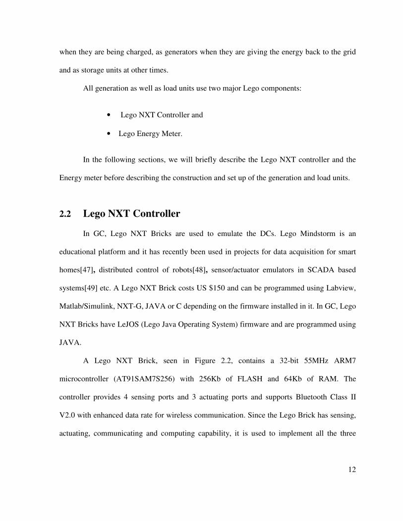
A Lego NXT Brick, seen in Figure 2.2, contains a 32-bit 55MHz ARM7

microcontroller (AT91SAM7S256) with 256Kb of FLASH and 64Kb of RAM. The

controller provides 4 sensing ports and 3 actuating ports and supports Bluetooth Class II

V2.0 with enhanced data rate for wireless communication. Since the Lego Brick has sensing,

actuating, communicating and computing capability, it is used to implement all the three

13

layers of the GC. Different software agents described below are introduced to carry out the

functions of each layer.

Output Ports

Input Ports

USB

Port

Interface Buttons

LCD Display

Figure 2.2: Lego NXT brick and the components within

2.3 Energy Meter/Energy Storage Device

Lego Energy Meter/Energy Storage Device (ESD) is a commercially available Lego

part that is used for sensing the voltage, current, power, and energy data. The ESD is

connected to one of the sensing ports of the NXT Brick and communicates the data at

specified rate using I2C communication protocol. The ESD also comes with a battery to act

as a temporary energy storage unit. The energy produced by the generation units is stored in

this buffer before being supplied to the grid. Figure 2.3 shows different parts of the Lego

Energy Meter:

14

• Mindstorm Output Port – Allows the ESD to be used with LEGO.

• Display – Shows input and output measurements, as well as power status

and error information. Figure 2.4 shows the details of the ESD Display.

• Directional control switch – Selects the output function. Set to the middle

position to turn the output function off. By controlling the switch, the ESD

can be used to charge or discharge the battery that is attached to the ESD.

More about this function is described in the following section.

• On/Off button – Turns the Energy Meter on and off. Press and hold for

two seconds to reset the joule counter.

• Output plug – Connect components, such as E-Motor and LED Lights, to

use the stored energy and measure the energy needed to power them.

• Input plug – Connect various power sources here to charge the Energy

Meter or Connect the Solar Panel or E-Motor, used as a generator and read

the Energy Meter measurements.

15

Figure 2.3: Lego Energy Meter/ Energy Storage Device (ESD)

Figure 2.4: ESD display

16

2.3.1 Directional Control Switch

The directional control switch can be controlled to charge or discharge the battery in

the ESD. In Green City, an automated switching mechanism is designed to either charge or

discharge the ESD battery. The automated actuation system is shown in Figure 2.5. This

actuation system helps to simulate a condition where a particular energy source needs to be

selected to supply the energy in the grid. For example, if at a particular moment the ESD on

the wind turbine has a full battery and the ESD on the conventional generators are running on

a low battery ideally we need to start charging the ESD’s on the conventional generators and

provide power to the grid from the ESD’s of the wind turbine. The electrical actuation system

allows for such flexibility in the system. We can control which energy source provides power

in the grid using the intelligent switching of energy source.

Figure 2.5: Automated actuation system of directional control switch

17

2.4 Generation Units

Three types of generation units are currently supported in the Green City – Wind

Turbine, Solar Panel and Conventional Generators.

2.4.1 Wind Turbine

Wind turbine is a renewable energy source. In Green City, a laboratory scale wind

turbine is emulated using components from Lego renewable energy package. Figure 2.6

shows a wind turbine in Green City.

Figure 2.6: Wind turbine in Green City

18

The wind turbines installed in Green City have the following components attached:

• Motor: To change the wind turbine blade direction so that they can face

the direction of wind.

• Generator: To generate the electricity.

• NXT: To control the actuation of the motor and read the data from the

ESD

• ESD: To store the electric energy generated by the wind turbine

Table 2-I shows the connections of the wind turbine to the NXT Brick. Two actuator

output ports and a sensor input port is utilized by the wind turbine.

Table 2-I: Wind turbine connections to NXT Brick

Parts Connected NXT Port No

Motor 1 (Orientation) Port A

Motor 2 (ESD Switching Motor) Port B

ESD Input 1

19

Figure 2.7 shows the schematic diagram of the components in wind turbine and their

connection to the NXT and other parts of Green City. A fan is used to generate the wind

which turns the blades of the wind turbine.

Wind Turbine

Generator

Figure 2.7: Wind turbine component connections

2.4.2 Solar Panel

Solar Panel is another renewable energy source. In Green City, a laboratory scale

solar panel is emulated using components from Lego renewable energy package. Figure 2.8

shows a solar panel in Green City.

20

Figure 2.8: Solar panel in Green City

The solar panels installed in Green City have the following components attached:

• Solar Panel: To generate the electricity.

• Motor: There are two motors installed on the Solar Panel.

o Motor 1: To control the pitch rotation of the panel.

o Motor 2: To control the tilt rotation of the panel.

• NXT: To control the actuation of the motors and read data from ESD.

21

• ESD: To store the electric energy generated by the solar panel.

Table 2-II shows the connections of the solar panel to the NXT Brick. Three actuator

output ports and a sensor input port is utilized by the solar panel. Two motors control the

pitch and the tilt of the solar panel to maximize the amount of electricity generated

Table 2-II: Solar panel connections to NXT Brick


Motor 1 (Tilt Angle) Port A

Motor 2 (Pitch Angle) Port B

Motor 3 (ESD Switching Motor) Port C

ESD Input 1

Figure 2.9 shows the schematic diagram of the components in solar panel and their

connection to the NXT and other parts of Green City. A lamp is used to emulate the sun that

supplies the light required by the solar panel to generate electricity.

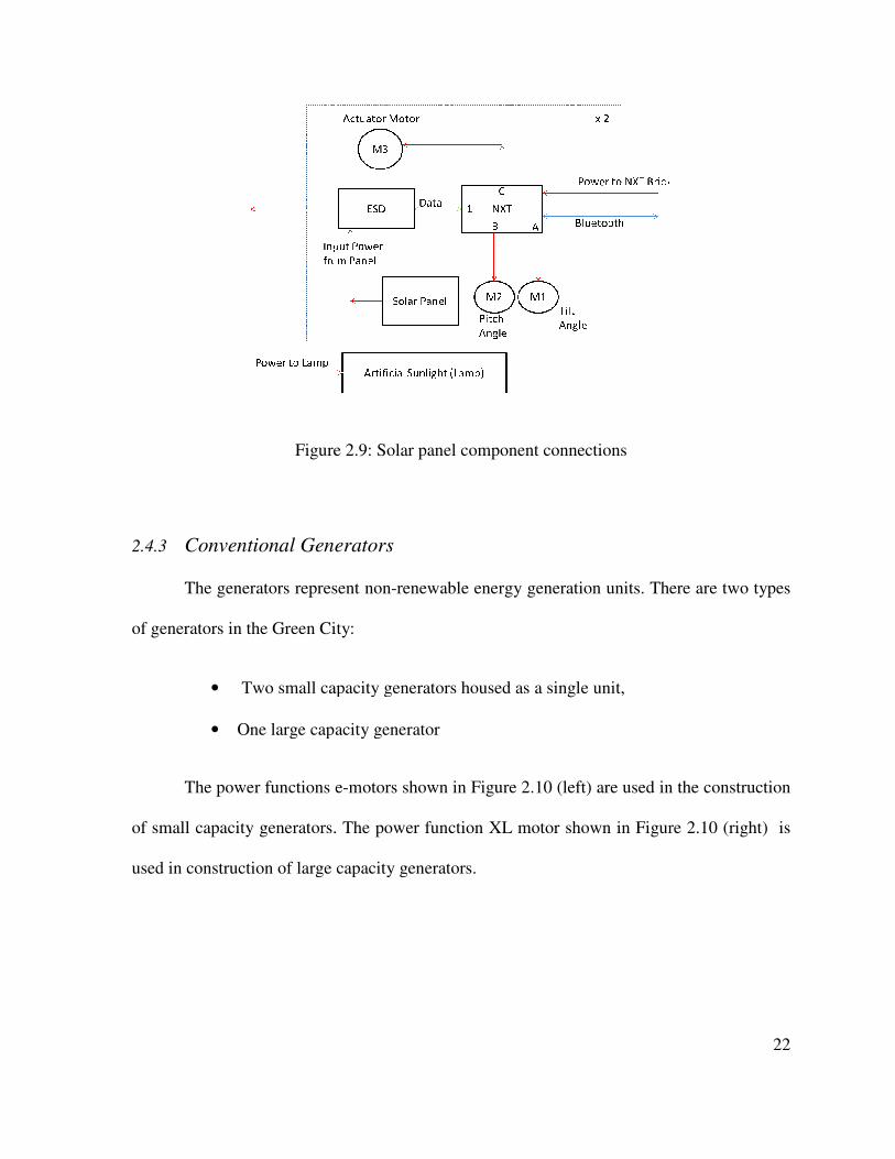
Figure

2.4.3 Conventional Generators

The generators represent non

of generators in the Green City:

• Two small capacity generators housed

• One large capacity generator

The power functions

of small capacity generators.

used in construction of large capacity generators

Figure 2.9: Solar panel component connections

Generators

The generators represent non-renewable energy generation units. There are two types

reen City:

Two small capacity generators housed as a single unit,

One large capacity generator

unctions e-motors shown in Figure 2.10 (left) are used in the construction

small capacity generators. The power function XL motor shown in Figure

used in construction of large capacity generators.

22

renewable energy generation units. There are two types

are used in the construction

Figure 2.10 (right) is

23

Figure 2.10: Power functions e-motor (left) and XL motor (right)

Figure 2.11: Small capacity generators in Green City

24

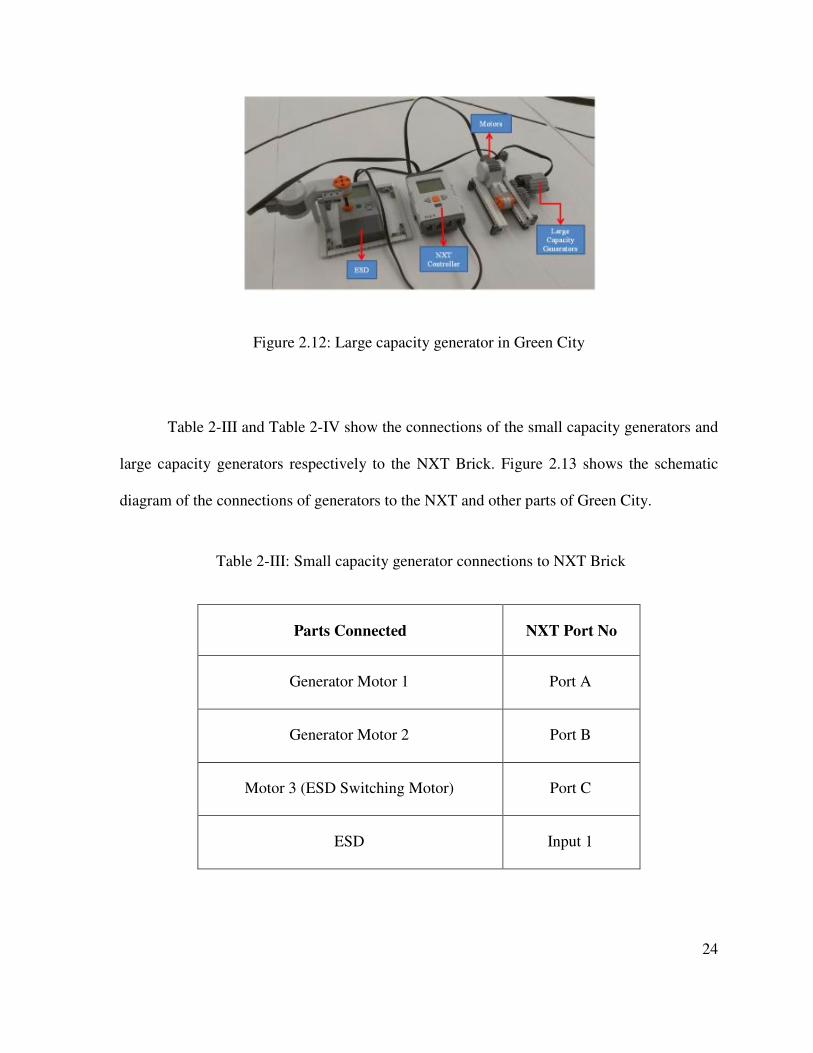
Figure 2.12: Large capacity generator in Green City

Table 2-III and Table 2-IV show the connections of the small capacity generators and

large capacity generators respectively to the NXT Brick. Figure 2.13 shows the schematic

diagram of the connections of generators to the NXT and other parts of Green City.

Table 2-III: Small capacity generator connections to NXT Brick


Generator Motor 1 Port A

Generator Motor 2 Port B


ESD Input 1

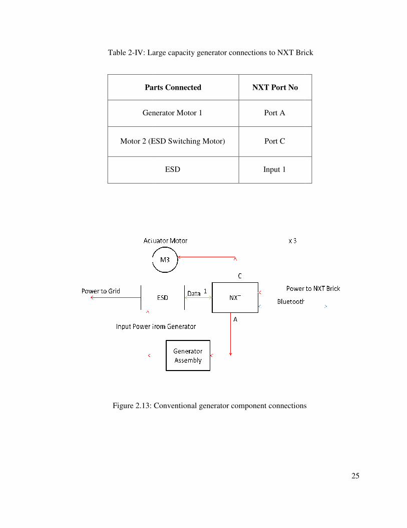
Table 2-IV: Large capacity generator connections to NXT Brick

Parts Connected

Generator Motor 1

Motor 2 (ESD Switching Motor)

Figure 2.13: Conventional

: Large capacity generator connections to NXT Brick


Generator Motor 1 Port A


ESD Input 1

: Conventional generator component connections

25

: Large capacity generator connections to NXT Brick

connections

26

2.5 Load units

Two types of loads are currently installed in the Green City platform – household and

charging stations.

2.5.1 Household

Figure 2.14 shows a household unit in the Green City. The household unit consists of

a NXT Brick which is connected to a series of LEDs through the sensor ports 1 and 2. The

amount of power consumed by the household unit depends on the number of LEDs that are

switched on. Currently two sensor ports are used to connect the LEDs to the NXT Brick.

Figure 2.14: Household unit in Green City

27

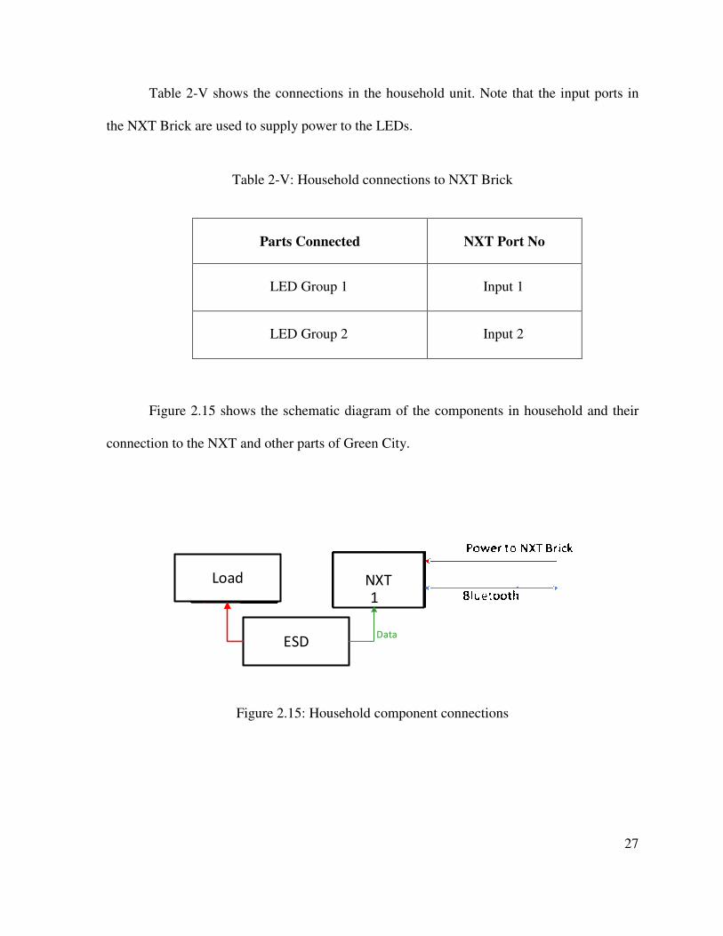
Table 2-V shows the connections in the household unit. Note that the input ports in

the NXT Brick are used to supply power to the LEDs.

Table 2-V: Household connections to NXT Brick


LED Group 1 Input 1

LED Group 2 Input 2

Figure 2.15 shows the schematic diagram of the components in household and their

connection to the NXT and other parts of Green City.

NXTLoad

ESD

1

Data

Figure 2.15: Household component connections

28

When the household unit needs to operate as a responsive load, the NXT controller

switches LED groups on or off according to the decision made in the control layer. When

household unit is used as a constant load, all LED units are switched on.

2.5.2 Charging Station

Charging station itself cannot act as a load. However, it acts as a load when electric

vehicles dock to the charging stations. Figure 2.16 shows a charging station in the Green

City. A charging station has the following major components:

• NXT: To connect to and get information about the electric vehicle being

charged in the charging station

Figure 2.16: Charging station in Green City

29

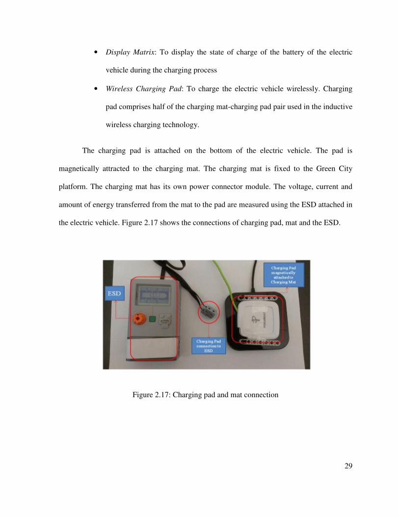
• Display Matrix: To display the state of charge of the battery of the electric

vehicle during the charging process

• Wireless Charging Pad: To charge the electric vehicle wirelessly. Charging

pad comprises half of the charging mat-charging pad pair used in the inductive

wireless charging technology.

The charging pad is attached on the bottom of the electric vehicle. The pad is

magnetically attracted to the charging mat. The charging mat is fixed to the Green City

platform. The charging mat has its own power connector module. The voltage, current and

amount of energy transferred from the mat to the pad are measured using the ESD attached in

the electric vehicle. Figure 2.17 shows the connections of charging pad, mat and the ESD.

Figure 2.17: Charging pad and mat connection

30

The display matrix is RGB LED Matrix with I2C Backpack which has an ATtiny

2313 to provide an I2Cinterface. This interface makes it possible for communication between

NXT and the LED Matrix. Table 2-VI shows the pin out connections of the display matrix.

Figure 2.18: Electrical vehicle docked in the charging station

31

Table 2-VI: Pin-out of the display matrix

Pin No Pin Name Pin Function

1,2,3 5V Logic and LED Power

4,6,8 GND Ground

5 SDA I2C Data

7 SCL I2C Clock

9-10 3V3 Not Connected

Communication with the board is done by sending 24 bytes to the board through I2C.

Each byte controls a single row of a single colour. First 8bytes control Red LED’s, next 8

bytes control Green LED’s and the final 8 bytes control Blue LED’s. Table 2-VII shows the

connections from NXT cable to the RGB LED Matrix.

32

Table 2-VII: Display matrix connections to NXT Brick

NXT Cable Wire LED Matrix Wire LED Matrix Pin

Ground (Black, Red) Grey, Blue, Yellow 4,6,8

+4.3 Supply (Green) Brown, Red, Orange 1,2,3

I2C Clock SCL (Yellow) Violet 7

I2C Data SDA (Blue) Green 5

Table 2-VIII shows the connections in the charging station unit. Note that the input

ports in the NXT Brick is configured as a I2C port to communicate with the display matrix.

Table 2-VIII: Charging station connections to NXT Brick


Display Matrix Input 1

Figure 2.19 shows the schematic diagram of the components in charging station and

their connection to the NXT and other parts of Green City.

33

NXT1Display Matrix

Figure 2.19: Charging station component connections

2.6 Electric Vehicle

Electric vehicle acts as a load in the Green City when it is docked in the charging

station. Figure 2.20 shows the electric vehicle constructed in the Green City platform. The

electric vehicle is also an automated ground vehicle that can go from one point to another

autonomously in the Green City. Thus the electric vehicle has components related to energy

monitoring as well as path tracking.

Figure 2.20: Front view of electric vehicle

34

The major components of the electric vehicle are:

• NXT: To control the motion of the robot, charging/discharging amount and

various other control tasks.

• Motors: To move the electric vehicle from one point to another (for

example to the charging station when the battery is low). The motors can

run up to a speed of 900 degrees/second when the battery is fully charged.

• Ultrasonic Sensor: To sense if there is an obstacle in from the the

automated electric vehicle. It can measures distance in centimeters ranging

from 0 to 255, with a precision of +/-3cm..

• Light Sensor: To provide the feedback when the electric vehicle is

tracking a black line. It measures the intensity of the reflected light. The

values range from 0 to 100 with 0 meaning darkness and 100 meaning

intense sunlight.

• Discharge Circuit: To simulate the a load for the electric vehicle. More is

described in the following sections.

• ESD: To simulate the battery of the electric vehicle and to monitor the

amount of charge/discharge of the battery.

• Battery Fuel Gauge: To display the SOC of the electric vehicle battery.

35

Table 2-IX: Electric vehicle connections to NXT Brick


Light Sensors (1-3) Input 1-3

Ultrasonic Sensor Input 4 (I2C)

Battery Fuel Gauge Input 4 (I2C)

Discharging Circuit Input 4 (I2C)

ESD Input 4 (I2C)

Motor 1 & 2 (Right and Left Wheel) Ports A and B

Motor 3 (Ultrasonic Sensor Movement) Port C

Table 2-IX shows the connections of the electric vehicle. Note that input port 4 is

used with four I2C devices. The nature of I2C communication allows multiple slaves to

connect to the master as long as the slaves have different address. NXT is acting as the

master in this scenario.

Figure 2.21 shows the schematic diagram of the manner in which the various

components were connected on the electric vehicle.

Figure 2.

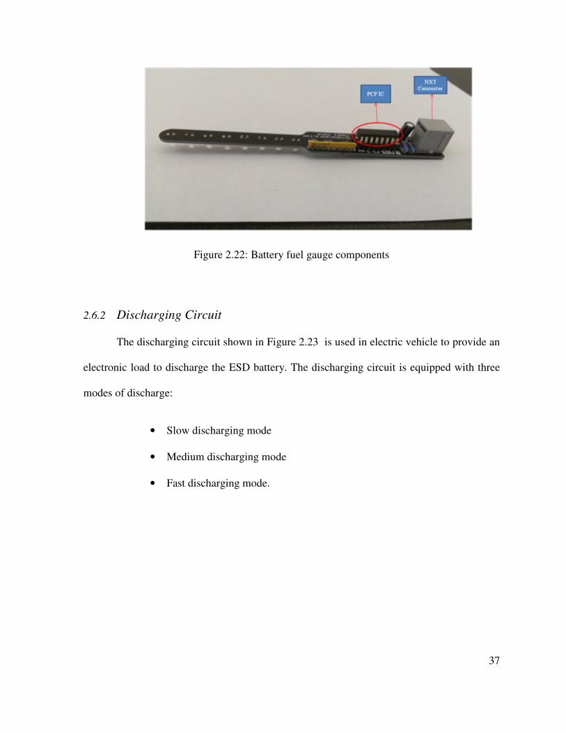
2.6.1 Battery Fuel Gauge

Figure 2.22 shows the battery fuel gauge

magic wand is to display the

PCF8574 chip. The PCF8574 provides general purpose remote I/O expansion for most

microcontroller families via the I2C interfa

using the user interface developed in the Le

control the output pins of the PCF8574

.21: Electric vehicle component connections

Battery Fuel Gauge

shows the battery fuel gauge in electric vehicle. The

magic wand is to display the state of charge of the ESD. It is constructed using LEDs and a

8574 provides general purpose remote I/O expansion for most

microcontroller families via the I2C interface. The communication with the PCF8574

using the user interface developed in the LeJOS software. We can send data in hex format to

trol the output pins of the PCF8574.

36

The function of the

It is constructed using LEDs and a

8574 provides general purpose remote I/O expansion for most

. The communication with the PCF8574 is done

software. We can send data in hex format to

37

Figure 2.22: Battery fuel gauge components

2.6.2 Discharging Circuit

The discharging circuit shown in Figure 2.23 is used in electric vehicle to provide an

electronic load to discharge the ESD battery. The discharging circuit is equipped with three

modes of discharge:

• Slow discharging mode

• Medium discharging mode

• Fast discharging mode.

38

Figure 2.23: Discharging circuit components

The discharging rate is controlled by using three LEDs in the discharging circuit.

PCF8574 is used to communicate with the NXT controller and control the LEDs. The LED

combination for different modes of discharge is given in Table 2-X.

Table 2-X: LED combination for different modes of discharge

Discharge Mode LEDs switched ON

Slow mode Green

Medium mode Orange & Red

Fast mode Green, Orange and Red

39

Figure 2.24 shows the schematic diagram of the discharging circuit. Figure 2.25

shows the physical layout of the actual components that are connected to the NXT controller

in the electric vehicle

VDD

PCF

8574

ORANGE LED GREEN LEDRED LED

R1 = 100 Ω

R1 = 150 Ω R1 = 150 Ω

R1 = 150 Ω

Nmos 1 Nmos 2 Nmos 3

R1 = 100 Ω

Figure 2.24: Discharging circuit schematic

40

Figure 2.25: Actual components on the electric vehicle and their connections

41

Chapter 3 Distributed Controllers

3.1 Introduction

Figure 3.1 shows the structure for the Green City (GC) platform. The Green City

consists of three major software components given below:

• Distributed Controller,

• The Router, and

• The Graphical User Interface (GUI),

In GC, smart grid is viewed as a multi-agent system where each energy device

interfaces and interacts with the power network through a distributed controller. Standard

interfaces/templates are defined for incorporating new algorithms, communication channels,

and energy devices to make GC a readily expandable fast-prototyping platform. The

integration of distributed controllers as well as the ability to perform tests under dynamic

communication and processing constraints separates GC from the existing platforms. Major

features of the GC are:

• Modularity – allows proper management of distributed system through the

use of three layered, agent based design for distributed controllers,

• Real-time Monitoring –has a graphical user interface that provides real-

time access of data to the operator, for monitoring and control tasks,

• Integration of Communication Constraints –allows testing and verification

42

under different communication constrains such as delay, communication

noise etc,

Graphical User Interface (PC)

Network/

Router Node n

...Node 2

Node 1

Setup Window Display Window

Distributed Controllers

Figure 3.1: Green City platform structure

43

• Fast Prototyping –allows user to promptly integrate changes in existing

algorithms and supports fast prototyping such that new algorithms can be

easily added into the system,

• Reconfigurability/Heterogeneity – allows each distributed controller in GC

to be easily reconfigured to interface with heterogeneous distributed

energy devices to facilitate interoperability,

• Flexibility –accommodates dynamic changes in network as well as

algorithm parameters, and

• Simplicity – uses simple, standard and easily available hardware.

Every architecture and design decision in GC platform is taken based on these seven

features. This chapter along with Chapter 4 will present the details about the architecture,

design and functional description of the software structure for the GC platform. While this

chapter will focus on the software design for the distributed controllers, chapter 4 will

discuss the details about graphical user interface and the router.

3.2 The Distributed Controllers

The future power system is a Cyber-Physical System (CPS) which is geographically

distributed and has a dynamic topology. It also integrates a variety of controllable energy

devices such as Distributed Generators (DG), Distributed Energy Storage Devices (DESD),

as well as controllable loads and responsive demands. This calls for a paradigm shift that

needs to consider the local intelligence of the distributed devices as well as their

44

communication capability [40]. As such each distributed generation, storage and load unit

needs to have a local controller which is capable of performing the following major tasks:

• Sense its own data such as voltage, current, power etc,

• Receive data from its neighbors,

• Perform simple computations to make control decisions based on its own

as well as its neighbor’s data,

• Actuate based control decisions taken, and

• Send information about its current state to its neighbors.

The distributed controller in the green city is designed to be the local controller for

the distributed generation, storage and load units. Figure 3.2 shows a conceptual diagram

showing the role of the distributed controller in the future power system. Each distributed

unit (generator, load, storage etc) is connected to the cyber network of the power system

through a distributed controller. The distributed controller should not only be able to perform

the tasks defined above but also provide a uniform interface between the heterogeneous

components in power system network.

45

Energy Storage

Device

Distributed

Controller

Distributed

Controller

Distributed

Controller

Distributed

Controller

Distributed

ControllerGenerator

Solar

Panel

Responsive

Load

Wind

Turbine

Figure 3.2: Distributed controllers in the future power system

The major tasks of the distributed controller can be functionally divided into three

categories:

• Sensing/Actuating

• Communication

• Control

The sensing/actuating functions concern with the distributed controller’s interaction

with the power system unit that it is physically connected to. The communication functions

concern with the distributed controller’s interaction with other distributed controllers. And

46

finally the Control functions concern with using the sensed and received data to make an

optimal decision for the power system unit.

This functional categorization of major tasks is an important factor in the design

decision for software architecture of the distributed controller in the Green City platform. In

order to make the platform modular, the software architecture of the distributed controller

consists of three layers - physical layer, communication/cyber layer, and control layer as

shown in Figure 3.3. Each layer communicates with other layer through the use of standard

data structure. This layered approach is used so that the modifications done in each layer are

independent of the other layers. Agents are used in each layer to further modularize the

Green City platform.

Sensing

Agent

Actuating

Agent

Data

Packaging

Agent

Routing

Agent

Disturbance

Agent

Data Receiving Agent

Configuration Agent

Functional Agent

Data Sending

Agent

Control

Decision

Neighbor

Data

Local

Sensor

Data

Physical Layer

Cyber/Communication Layer

Control Layer

Figure 3.3: Three layered software architecture for distributed controllers

47

3.2.1 Physical Layer

The physical layer of the system is responsible for providing the interface for sensing

and actuating processes. Two agents used in this layer are Sensing Agent and Actuating

Agent.

3.2.1.1 Sensing Agent

Each distributed controller has a sensing agent which acts as the interface between the

sensors and the rest of the system. The major task of the sensing agent is to add, remove,

initialize and read the data from the sensors. Figure 3.4 shows the class structure of the

sensing agent. SensorAgent can contain one or more Sensors.

SensorAgent

- SensorList[]

...

- setSampl ingInterval(int samplingInterval)

- addSensor(Sensor S, int portID)

- initializeSensor(int samplingInterval)

- getSensorReading(Sensor S)

- getAllSensorData()

...

Sensor

- name

- portID

- samplingInterval

- currentReading

...

- senseData()

- setSamplingInterval(int samplingInterval)

...

EnergyMonitor

- i2cAddress

...

- senseData()

...

AbsoluteEncoder

...

- senseData()

...

1..*

Figure 3.4: Sensing agent and the sensor class

48

Note that Sensor is designed as an abstract class. The methods those are invariant for

different sensor (such as setSamplingInterval() is already implemented in the Sensor class.

However, some methods such as senseData() are kept as abstract method because the process

of reading a sensor’s data may differ from one sensor to another. For example the method of

decoding the I2C data from energy sensor will be much different than the method for reading

the absolute encoder values from the motors. As such, senseData() method is uniquely

implemented by all the concrete classes that implement the abstract class.

3.2.1.2 Actuating Agent

Similar to the sensing agent, each distributed controller has an actuating agent. As

seen in Figure 3.5, the structure of the actuator agent is similar to the structure of the sensing

agent. Each ActuatorAgent can have one or more Actuators. Any set-up or control command

to the Actuator has to come through the ActuatorAgent. The setActuatorValue sets the

currentOutput for the Actuator which is used by the actuate method in the concrete Actuator

class. As with the Sensor class, the Actuator class is an abstract class which contains both

abstract as well as normal methods. Currently, only one actuator (Motor) has been set up in

the Green City platform. However, the standard template for the Actuator is designed such

that adding any other actuator can be done easily by implementing the actuate() method

along with any additional method that the new actuator may need. This supports modularity

in the system.

49

ActuatorAgent

- ActuatorList[]

...

- setActuatingInterval(int samplingInterval)

- addActuator(Actuator A, int portID)

- initializeActuator(int samplingInterval)

- setActuatorValue(Actuator A, double Val)

...

Actuator

- name

- portID

- samplingInterval

- currentOutput

...

- actuate()


...

Motor

...

- actuate()

...

1..*

Figure 3.5: Actuator agent and actuator class

3.2.2 Communication/Cyber Layer

The communication/cyber layer is responsible for sending and receiving data between

distributed controllers. In order to perform these tasks, four agents are introduced – Data

Packaging Agent, Routing Agent, Data Sending Agent, and Data Receiving Agent. Each

agent is described in detail in the following section. In addition to these four agents, another

agent called Disturbance Agent is also defined that allows the operator to inject

communication constraints such as delay, packet loss and noise.

3.2.2.1 Data Packaging Agent

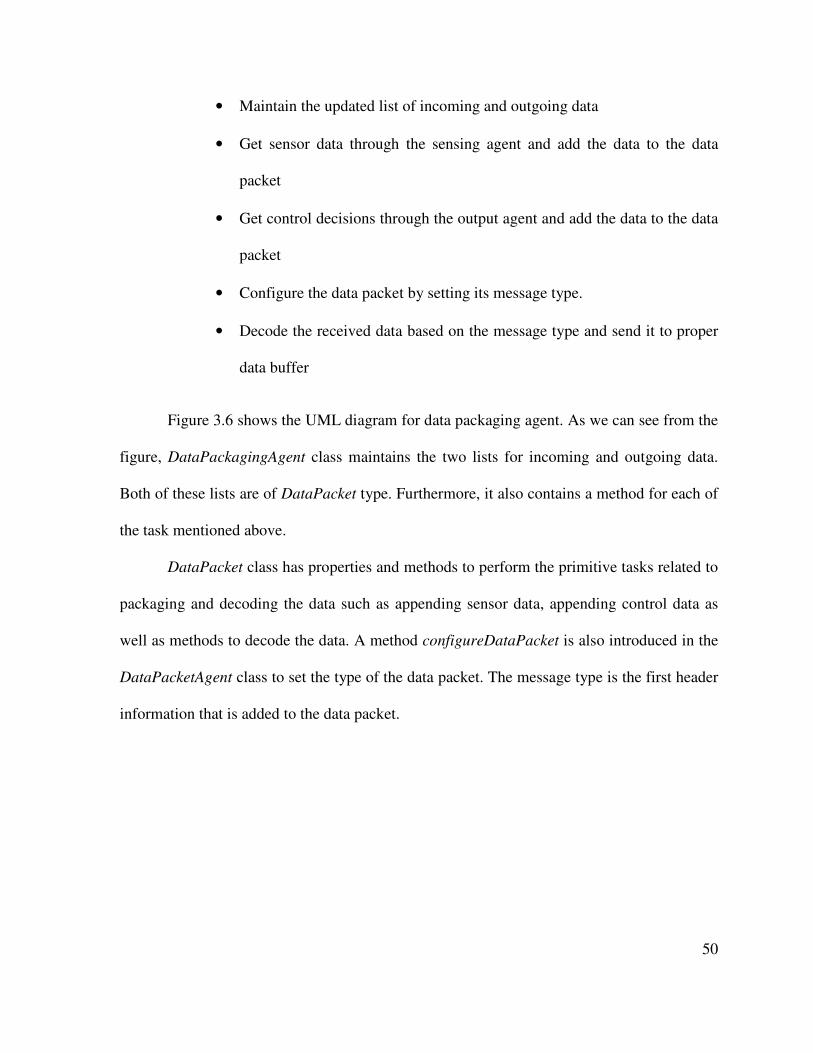
Data packaging agent has the following major tasks

50

• Maintain the updated list of incoming and outgoing data

• Get sensor data through the sensing agent and add the data to the data

packet

• Get control decisions through the output agent and add the data to the data

packet

• Configure the data packet by setting its message type.

• Decode the received data based on the message type and send it to proper

data buffer

Figure 3.6 shows the UML diagram for data packaging agent. As we can see from the

figure, DataPackagingAgent class maintains the two lists for incoming and outgoing data.

Both of these lists are of DataPacket type. Furthermore, it also contains a method for each of

the task mentioned above.

DataPacket class has properties and methods to perform the primitive tasks related to

packaging and decoding the data such as appending sensor data, appending control data as

well as methods to decode the data. A method configureDataPacket is also introduced in the

DataPacketAgent class to set the type of the data packet. The message type is the first header

information that is added to the data packet.

51

DataPackagingAgent

- incomingDataPacketList

- outgoingDataPacketList

...

- appendSensorData(SensingAgent S)

- appendControlData(OutputAgent O)

- configureMessageType(int messageID)

- decodeData(DataPacket d)

...

DataPacket

- destinationID

- sourceID

- messageType

- data

...

- appendData(String data)

- appendHeader()

...

1..*

Figure 3.6: Data packaging agent and data packet class

Different message types can be received or sent by a distributed controller. The

decoding/encoding process of the data packet differs based on the type of the message. Table

3-I shows the different types of messages that are currently used in the Green City platform.

Since Green City is a research platform, most of these messages are messages coming from

the GUI where the operator/researcher is setting the parameters related to the network

structure, algorithm initialization, algorithm selection, synchronization, leader identification

and initialization etc. After this initialization phase, the distributed controller receives

neighbour data whose message id is 6.

52

Table 3-I: Message types currently used in the Green City platform

Message Type Message ID

MESSAGE_DISCONNECT 0

MESSAGE_EXIT 1

MESSAGE_CONTROL 2

MESSAGE_ALGORITHMTYPE 3

MESSAGE_PARAMUPDATE 4

MESSAGE_STARTALGO 5

MESSAGE_NEIGHBORDATA 6

MESSAGE_REQALGODATA 7

MESSAGE_REQNODEDATA 8

MESSAGE_STOPALGO 9

MESSAGE_NODEPARAMS 10

MESSAGE_LEADERINFO 11

53

3.2.2.2 Routing Agent

Because of the distributed nature of the future power system, a distributed controller

needs to communicate only with its neighbours. In the Green City platform, the operator

decides the network topology. The up-to-date network topology information is stored by the

distributed controller using the Routing Agent. Figure 3.7 shows the routing agent. As we

can see, RoutingAgent contains routingTable and networkParams which contain the updated

parameters related to network topology and behaviour. Methods also exist to update the

network related parameters. RoutingAgent is used to set the source and destination ID for the

data packet that is to be sent from the distributed controller.

RoutingAgent

- routingTable

- networkParams

...

- configureDataPacket()

- updateRoutingTable(String d)

- updateNetworkParams(String s)

...

Figure 3.7: Routing agent

3.2.2.3 Data Sending Agent

Data sending agent is responsible for sending the data to the neighbours at specified

sampling interval. Depending on the communication medium that is being used, data sending

54

process could differ; therefore, a data sending agent should act as the standard interface

between the actual protocol used to send the data and the rest of the system. Even though the

Green City platform uses Bluetooth communication between the distributed controllers, the

data sending agent is designed such that it can be easily expanded to use other network

protocols. CommChannel is the abstract class that should be inherited by all the concrete

communication channel classes. Each of these classes should implement the three basic

operations in the commChannel class – connect(), sendData(), and receiveData().

DataSendingAgent

- communicationChannel

...


- appendHeader(DataPacket d)

- sendData(DataPacket d)

...

CommunicationChannel

- incomingBuffer

- outgoingBuffer

- samplingInterval

...

- connect()

- sendData(String s)

- receiveData()


...

Bluetooth

- btConnection

...

- connect()


- receiveData()

...

1

Figure 3.8: Data sending agent and the communication channel class

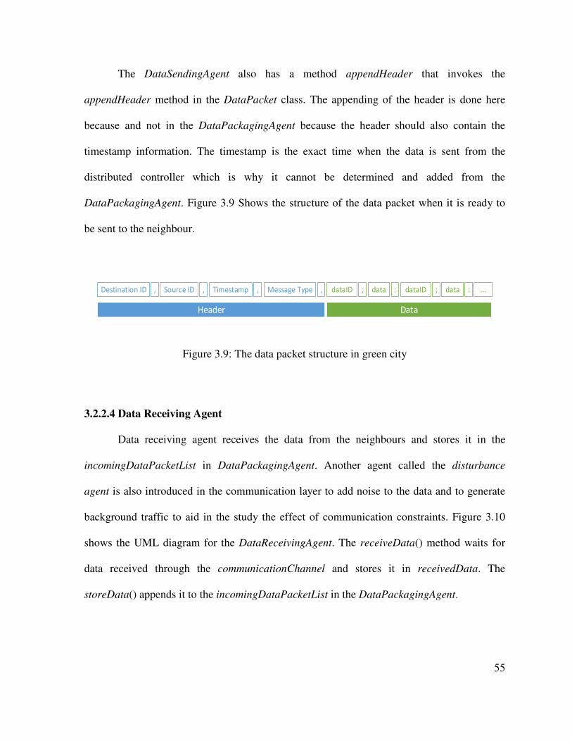
55

The DataSendingAgent also has a method appendHeader that invokes the

appendHeader method in the DataPacket class. The appending of the header is done here

because and not in the DataPackagingAgent because the header should also contain the

timestamp information. The timestamp is the exact time when the data is sent from the

distributed controller which is why it cannot be determined and added from the

DataPackagingAgent. Figure 3.9 Shows the structure of the data packet when it is ready to

be sent to the neighbour.

Destination ID Source ID dataID, Message Type, , ; data dataID: ; data : ...Timestamp ,

DataHeader

Figure 3.9: The data packet structure in green city

3.2.2.4 Data Receiving Agent

Data receiving agent receives the data from the neighbours and stores it in the

incomingDataPacketList in DataPackagingAgent. Another agent called the disturbance

agent is also introduced in the communication layer to add noise to the data and to generate

background traffic to aid in the study the effect of communication constraints. Figure 3.10

shows the UML diagram for the DataReceivingAgent. The receiveData() method waits for

data received through the communicationChannel and stores it in receivedData. The

storeData() appends it to the incomingDataPacketList in the DataPackagingAgent.

56

DataReceivingAgent

- communicationChannel

- receivedData

...


- storeData()

- receiveData()

...


- incomingBuffer

- outgoingBuffer

- samplingInterval

...

- connect()


- receiveData()


...

Bluetooth

- btConnection

...

- connect()


- receiveData()

...

1

Figure 3.10: Data receiving agent and the communication channel class

3.2.2.5 Disturbance Agent

Disturbance agent has three major tasks:

• To inject delay in the outgoing data packet by introducing background

traffic

• To emulate packet loss by dropping the data packet

• To inject noise based on the mean and variance set by the operator

As shown in Figure 3.11, the disturbance agent has properties to store the parameters

sent from the operator and has methods to inject the disturbance when necessary. The

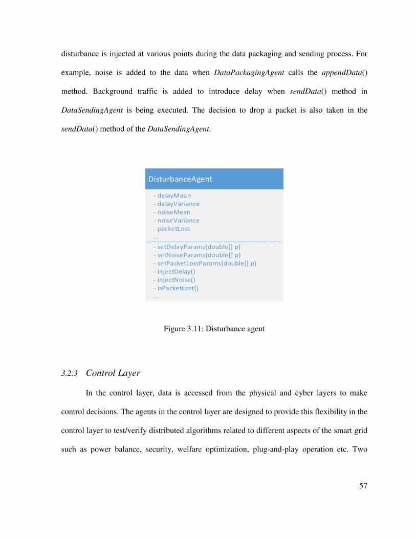
57

disturbance is injected at various points during the data packaging and sending process. For

example, noise is added to the data when DataPackagingAgent calls the appendData()

method. Background traffic is added to introduce delay when sendData() method in

DataSendingAgent is being executed. The decision to drop a packet is also taken in the

sendData() method of the DataSendingAgent.

DisturbanceAgent

- delayMean

- delayVariance

- noiseMean

- noiseVariance

- packetLoss

...

- setDelayParams(double[] p)

- setNoiseParams(double[] p)

- setPacketLossParams(double[] p)

- injectDelay()

- injectNoise()

- isPacketLost()

...

Figure 3.11: Disturbance agent

3.2.3 Control Layer

In the control layer, data is accessed from the physical and cyber layers to make

control decisions. The agents in the control layer are designed to provide this flexibility in the

control layer to test/verify distributed algorithms related to different aspects of the smart grid

such as power balance, security, welfare optimization, plug-and-play operation etc. Two

58

agents are defined for the functioning of the control layer – Configuration Agent and

Functional Agent.

3.2.3.1 Configuration Agent

Distributed controller should be designed such that it acts as the uniform, interface

between the generation/storage/load unit and the power system network. It should be

designed with the flexibility to work with any heterogeneous unit that is present in the power

system network. In order to do make the distributed controller flexible, ConfigurationAgent

is introduced in the Green City platform. Figure 3.12 shows the UML diagram of the

Configruration agent and the classes it is associated to. The major task of the

ConfiguraationAgent is to set up the types and ports for the sensors and actuators that a

specific distributed unit will use. An abstract Node class is introduced to standardize the

distributed unit type. The abstract Node class has defined a set of methods and properties to

properly set up the distributed controller. In addition to setting up sensors and actuators using

the setupSensors() and setupActuators() method, the functions to properly respond to the data

and control request is also defined in the abstract node class. Currently, five concrete classes

implement the Node class – WindTurbine, SolarPanel, Generator, ElectricVehicle, and Load.

59

ConfigurationAgent

- thisNode

...

- setupNode(int i)

...

Node

- nodeType

- nodeID

- sensingAgent

- actuatingAgent

...

- handleControlReq(String s)

- handleDataReq(String s)

- setupSensors(String s)

- setupActuators(String s)

...

WindTurbine

...





...

SolarPanel

...





...

1

Generator

...





...

ElectricVehicle

...





...

Load

...





...

Figure 3.12: Configuration agent and node class

Table 3-II shows the list of actuators and sensors for each type of node.

3.2.3.2 Functional Agent

Functional Agent is another agent in the control layer that is designed to make the

Green City platform flexible as well as generic. Since Green City platform is a laboratory

prototype for the smart grid, it should be designed to allow fast prototyping of the algorithms

related to different aspects of the smart grid such as optimal power generation, security, plug-

and-play capability etc. Figure 3.13 shows the UML diagram for the functional agent in the

Green City. The FunctionalAgent class itself is very simple which performs 3 major tasks

• Setup the algorithm to use

60

• Start the algorithm

• Stop the algorithm

Table 3-II: The set of sensors and actuators used by each node type

Node Sensor Actuator

WindTurbine

1 EnergyMeter (voltage, current)

1 AbsoluteEncoder(Motor position)

1 Motor (Orientation of the

Windmill)

SolarPanel

EnergyMeter (voltage, current)

Absolute Encoders (Motor position)

2 Motors (Yaw and pitch of

the Solar Panel)

Generator EnergyMeter(voltage, current) None

ElectricVehicle

EnergyMeter(voltage, current)

Absolute Encoders (position)

2 Motors (Left and Right

wheel)

Load

(Charging

Station)

EnergyMeter(voltage, current) None

61

setupAlgorithm() determines the algorithm that is to be run based on the choices made

by the operator. startAlgorithm() and stopAlgorithm() start or stop the algorithm based on the

operator’s choice.A standard is defined for the algorithms using the abstract

DistributedAlgorithm class. The DistributedAlgorithm class defines the following methods

• updateParameters() - update the parameters related to the algorithm. Data

is received from the operator. Different algorithms may have different sets

of parameters.

• updateNeighborData() - update the values of the neighbour’s data.

• updateLocalData() - update the values of the locally sensed data.

• compute() - perform the calculations to update the control data.

Five distributed algorithms have been implemented in the Green City –

• Consensus,

• Leader-Follower Incremental Cost Consensus,

• Secure Incremental Cost Consensus,

• Two Level Incremental Cost Consensus, and

• Incremental Welfare Algorithm.

62

DistributedAlgorithm

- algorithmType

- node

- localData

- neighborData

- controlData

...

- updateParameters(String s)

- updateNeighborData()

- updateLocalData()

- compute()

...

Consensus

...



- compute()

...

Leader-Follower Incremental Cost

Consensus (LFICC)

...



- compute()

...

1

Secure ICC

...



- compute()

...

Incremental Welfare Consensus (IWC)

...



- compute()

...

Two Level ICC

...


- - updateNeighborData()

- compute()

...

FunctionalAgent

- distributedAlgorithm

...

- setupAlgorithm(int i)

- startAlgorithm()

- stopAlgorithm()

...

Figure 3.13: Functional agent and related classes

63

Chapter 4 Graphical User Interface

4.1 Introduction

The graphical user interface (GUI) is another important component of the Green City

platform. It is through the use of GUI that real-time monitoring is made possible. GUI plays

an important role in setting up the system to run under specific scenarios chosen by the

operator. Since Green City is a laboratory platform used for R&D purpose, it is very

important that the operator/researcher has complete control and visibility of the Green City

environment. Using the GUI in Green City, the operator will be able to:

• Setup network topology,

• Setup/configure the distributed controllers (DCs)

• Setup algorithm parameters,

• Choose simulation/experimental platform,

• Setup communication constraints,

• Display states/control values of single DC or several DCs, and

• Log/save data for future analysis.

4.2 Software Architecture

Figure 4.1 shows the software architecture of the Green City GUI. Agent based

structure is used to implement the Model-View-Controller (MVC) design pattern. MVC

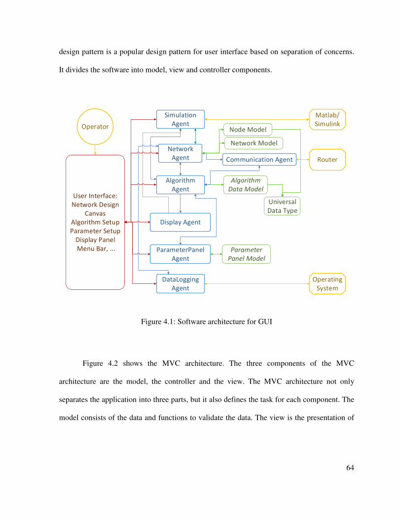
64

design pattern is a popular design pattern for user interface based on separation of concerns.

It divides the software into model, view and controller components.

User Interface:

Network Design

Canvas

Algorithm Setup

Parameter Setup

Display Panel

Menu Bar, ...

Network

Agent

Display Agent

Algorithm

Agent

Simulation

Agent

Communication Agent

DataLogging

Agent

Router

Algorithm

Data Model

Node Model

Universal

Data Type

ParameterPanel

Agent

Operating

System

Matlab/

Simulink

Parameter

Panel Model

Operator

Network Model

Figure 4.1: Software architecture for GUI

Figure 4.2 shows the MVC architecture. The three components of the MVC

architecture are the model, the controller and the view. The MVC architecture not only

separates the application into three parts, but it also defines the task for each component. The

model consists of the data and functions to validate the data. The view is the presentation of

65

the data. It can be in several forms such as text, plot or a diagram. A controller receives,

interprets and validates the input and updates/modifies the other components of the MVC

architecture. For e.g. it can send commands to its related view to change the plot or to update

the data in the model. A model can notify the controller when a change has occurred in its

state. This notification can trigger an update in the view or controller. In most cases, the

model does not actively notify the controller and/or view components but responds to

requests/queries from controller with appropriate data. The view requests the data from the

model through the controller for representation.

ModelData

representation,

storage, validation

ViewDisplay and

interface

ControllerReceive, interpret and

validate input,

create and update views,

query and modify models

User

operator

SeesUses

Manipulates,

Queries

UpdatesNotifies

Figure 4.2: Model-View-Controller architecture

66

4.3 Model Components in Green City GUI

The GUI in Green City maintains four models – algorithm data model, parameter

panel model, the network model and the node model.

4.3.1 The Algorithm Data Model

The algorithm data model is the warehouse for all the state/output data related to the

currently running algorithm. It is the repository for data from all distributed controllers. The

algorithm data model uses a universal data type to be able to store different types of data

related to different types of algorithms and distributed controllers. The structure of the

UniversalDataType class is given in Figure 4.3. UniversalDataType contains properties such

as the logical name of the data, its unit, the id that is used during communication, the

dimension of the data and a list containing the values of the data. It contains methods to get

and set the value of the data, to get the entire data in the form of an array or to copy another

array to the data type. Algorithm data model contains a list of UniversalDataType objects.

The size of the list depends on the algorithm in use and the number of active distributed

controllers.

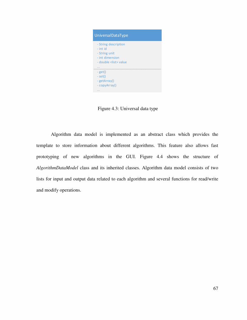
67

UniversalDataType

- String description

- int id

- String unit

- int dimension

- double <list> value

...

- get()

- set()

- getArray()

- copyArray()

...

Figure 4.3: Universal data type

Algorithm data model is implemented as an abstract class which provides the

template to store information about different algorithms. This feature also allows fast

prototyping of new algorithms in the GUI. Figure 4.4 shows the structure of

AlgorithmDataModel class and its inherited classes. Algorithm data model consists of two

lists for input and output data related to each algorithm and several functions for read/write

and modify operations.

68

AlgorithmDataModel

- UniversalDataType <list> inputData

- UniversalDataType <list> outputData

...

- initData()

- getParams()

- storeParams()

- sendParams()

- addRealTimeData()

- readParams()

...

ConsensusDataModel

...

- initData()

...

LFICCDataModel

...

- initData()

...

SecureICCDataModel

...

- initData()

...

IWCDataModel

...

- initData()

... TwoLevelICCDataModel

...

- initData()

...

Figure 4.4: Algorithm data model

• initData() – It is an abstract method that initializes the size, type, unit etc

of each state/output for an algorithm. Each algorithm will have different

types of parameters thus it is implemented as an abstract method.

• getParams()- This method is responsible for getting the algorithm input

parameters from the parameter panel.

• sendParams() – This method is sends the parameters to the controller for

further processing.

69

• addRealTimeData()- This method is used to add real-time data to the

universal data type list. It is called by the controller component whenever

new data is received from the distributed controllers

• readParams()- This is equivalent to addRealTimeData() except that it gets

the data from the Matlab workspace whenever a simulation is being run.

4.3.2 The Parameter Panel Model

The parameter panel model stores the information about the type and number of input

required by each algorithm. It cannot be changed during the run time; however, the operator

can however make changes to the model during compile time. The parameter panel is

populated based on this model. The parameter panel is composed of three different types of

input objects – the text input box, the selection box and the checkbox. The text input box

takes a numeric value, the selection box allows user to choose one among several distributed

controller (for e.g. choosing the leader node) and the checkbox input allows optional

properties to be set. Similar to the algorithm data model, the parameter model is also

implemented as an abstract class. This feature allows the model to be easily expandable to

incorporate new algorithms in the future. Figure 4.5 shows the structure of the

ParamPanelModel. The parameter panel model contains string lists to store the name and

description of the text fields, selection boxes and checkboxes. It also contains the list of

textfield, combobox and checkbox objects which are drawn in the parameter panel according

to the information stored in the textFields, selectionBoxes and checkBoxes. Several methods

are introduced to manage the parameter panel model.

70

ParamPanelModel

- String <list> textFields

- String <list> selectionBoxes

- String <list> checkBoxes

- JTextField <list> txtParams

-JComboBox <list> cmbParams

- JCheckBox <list> chkParams

- int[] varType

-...

- setTextFieldNames()

- setComboBoxNames()

- setCheckBoxNames()

- setDefaultValues()

- setupParamPanel()

-...

ConsensusPanelModel

...





LFICCPanelModel

...





SecureICCPanelModel

...





IWCPanelModel

...





TwoLevelICCPanelModel

...





Figure 4.5: Parameter panel model

• setTextFieldNames()- This is an abstract method that is implemented by

each algorithm to include the names of all the textbox type inputs to the

algorithm. All new algorithms should implement this method to notify the

application about the name and number of textbox type input to show in

the parameter settings panel.

• setComboBoxNames()- This is an abstract method which is implemented

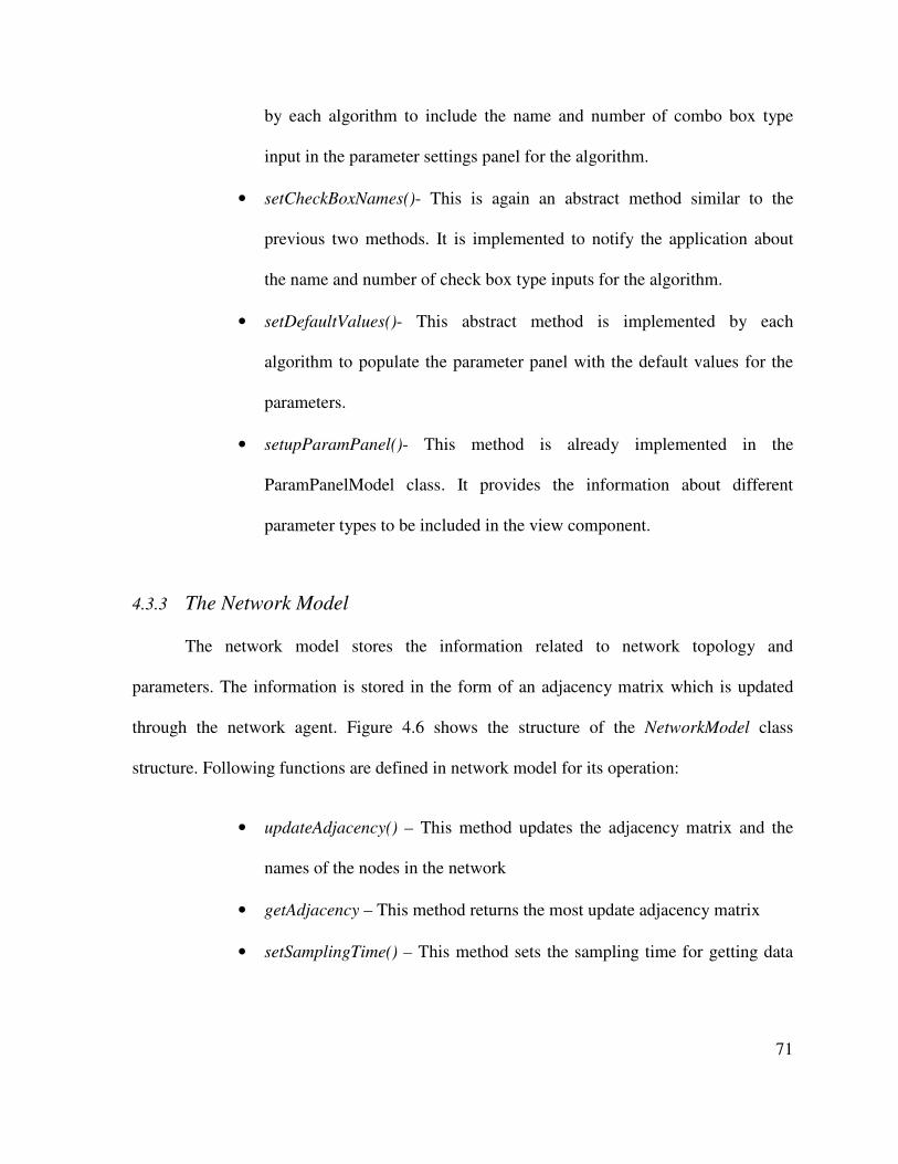
71

by each algorithm to include the name and number of combo box type

input in the parameter settings panel for the algorithm.

• setCheckBoxNames()- This is again an abstract method similar to the

previous two methods. It is implemented to notify the application about

the name and number of check box type inputs for the algorithm.

• setDefaultValues()- This abstract method is implemented by each

algorithm to populate the parameter panel with the default values for the

parameters.

• setupParamPanel()- This method is already implemented in the

ParamPanelModel class. It provides the information about different

parameter types to be included in the view component.

4.3.3 The Network Model

The network model stores the information related to network topology and

parameters. The information is stored in the form of an adjacency matrix which is updated

through the network agent. Figure 4.6 shows the structure of the NetworkModel class

structure. Following functions are defined in network model for its operation:

• updateAdjacency() – This method updates the adjacency matrix and the

names of the nodes in the network

• getAdjacency – This method returns the most update adjacency matrix

• setSamplingTime() – This method sets the sampling time for getting data

72

from diatributed controllers in the network

• getSamplingTime() – This method returns the current sampling time.

NetworkModel

- int [][] adjacencyMatrix

- String nodeNames

- int samplingTime

...

- updateAdjacency()

- getAdjacency()

- setSamplingTime()

- getSamplingTime

...

Figure 4.6: Network model

4.3.4 The Node Model

The node model stores the information about the node/distributed controller. It

includes the information about the type of energy device that the distributed controller is

connected to, the parameters of the energy device relevant to each algorithm; the status of the

node (active or inactive) etc. Figure 4.7 shows the NodeModel class structure.

73

NodeModel

- UniversalDataType <list> nodeParams

- String nodeID

- int nodeType

...

- updateNodeParams()

- getNodeParams()

...

Figure 4.7: Node model

Following functions are defined in the node model:

• updateNodeParams()- This method updates the properties related to the

node such as its type, parameters etc

• getNodeParams()- This method returns the desired parameter of the node.

4.4 View Components in Green City GUI

The GUI is developed using JAVA programming language and runs in the PC of the

operator/researcher. It has two parts:

• The setup window and

• The display window.

In the setup window, the operator can design/save/load network topology, select

simulation/experimental platform, select and setup algorithm parameters, and start running

74

the experiment/simulation. The setup window allows the operator to change the parameters

while the experiment is running thus allowing him to add/delete new nodes, inject faults,

introduce security threats, and change parameters during runtime. The display window

allows the user to monitor and save the state and control data of a single DC or a group of

DCs in real-time.

4.4.1 Setup Window

Figure 4.8 shows setup window of the GUI. There are eight major components in the

GUI - menu bar, distributed controller selection panel, network design canvas, command log,

network topology setup and display panel, algorithm and platform setup panel, action panel,

and algorithm parameter setup panel.

75

1

2

3

4

6

7

8

1 2 3 4

5 6 7

Menu Bar

Topology Setup/Display

Panel

Distributed Controller Selection Network Design Canvas Command Log

5

Algorithm/Platform Setup Panel

Action Panel 8 Parameter Setup Panel

Figure 4.8: Green City GUI setup window

4.4.1.1 Menu Bar

The menu bar consists of seven menu items. Figure 4.9 shows different menu items

and sub menu items in the menu bar.

76

• File – File menu contains commands to load data and network

configurations as well as commands to save current data and network

configuration for future use. Both loading and saving are done on a

sequential text file that contains the network, parameter and algorithm

information. The first section of the file contains the network topology

information saved as an adjacency matrix. The second section contains the

algorithm information and finally the third section of the file contains the

parameter information.

• Network – Network menu contains commands to load different kinds of

networks. Currently, 5 different kinds of network topology can be loaded

automatically – ring, star, chain, completely connect and randomly

generated topology. The menu also has a command to clear the currently

active network.

• Algorithms- Algorithms menu has two commands that allow the user to

use default parameters for each algorithm parameter or to set initial

parameters according to operator’s choice.

• Experiment – Experiment menu allows the operator to configure available

distributed controllers. Only the distributed controllers that are switched

on and within the range of the Bluetooth communication can be connected

to the PC thus it is important to set it up to notify which distributed

controllers are currently in range and active. This menu also allows the

operator to connect to the available nodes at any time during the run.

77

• Communication – Communication menu allows the operator to add

communication constraints such as noise, delay and packet loss to the

system. Furthermore, it also allows the operator to choose time based

setup or event based setup. In time-based setups, the distributed controllers

send data packets at a specified communication sampling time. In event

based setup, the controllers send the data when an event occurs. For

example receiving a data request can be a event which can trigger data

sending action.

• Display – Display menu allows the user to open the plots in the Matlab

figures

• Help- Help menu gives generic information about the Green City version

and copyrights.

78

Figure 4.9: Menu items in menu bar

4.4.1.2 Distributed Controller Selection Panel

Green City platform supports heterogeneous energy storage and generation units. The

distributed controller selection panel keeps record of currently active distributed controllers

(DCs) in the field. For example if a DC configured to be used with wind turbine is active on

the field, the wind turbine icon distributed controller selection panel is green, otherwise it is

gray. The operator can drag the wind turbine icon from the distributed controller selection

79

panel to the network design canvas to set up a network topology. If all the available DCs of a

particular type have been added to the network design canvas then the icon for that DC will

be gray.

4.4.1.3 Network Design Canvas

The network design canvas allows the operator to design and modify the network

topology. The operator can add edges DCs in the network design canvas to setup a

communication link between these two DCs in the actual physical world. The operator can

also modify individual properties of DCs by double clicking on the DCs. Double clicking the

DCs will open a popup window which allows changes in the DC properties. These properties

may change according to the algorithm that is currently in use. Right clicking on the DCs in

the network design canvas allows modification on the communication constraints for the DC.

A DC can be moved or deleted using the network design canvas. Every action done in the

network design canvas is logged in the command log. Changes in the network topology that

are done in the network design canvas are tracked/updated by using an adjacency matrix for

the network.

4.4.1.4 Command Log

Command log logs all the actions performed in the GUI. The actions include

adding/removing DC in network design canvas, adding/removing an edge from the network

design canvas, using any command from the menu bar, changing platform or algorithm,

80

updating or clearing the adjacency matrix, running/pausing or stopping an experiment,

updating algorithm parameters etc.

4.4.1.5 Network Topology Display/Setup Panel

This panel displays the updated adjacency matrix related to the network topology

designed using the network design canvas. It also allows the operator to upload an arbitrary

adjacency matrix for use in the experiment.

4.4.1.6 Algorithm and Platform Selection Panel

One of the major features of Green City GUI is that it not only facilitates real-time

control and monitoring of distributed controllers, but it also allows the operator to run

existing simulations in Matlab to compare the results from simulation and experiment. Thus,

in this panel, the operator will be allowed to choose the platform where he wants to run the

experiment. If he chooses simulation platform, GUI allows connection to Matlab and passes

the network topology and the algorithm parameters that have been set up in the GUI to

Matlab for execution. Upon completion of the execution the GUI gets a notification and

imports the results from Matlab for display. The operator can then run the same scenario

using the experimental platform by selecting experiment in the platform selection panel.

Once the results are received, the operator will be able to compare the results of the

simulation and experiment.

The algorithm selection panel allows the operator to choose between the algorithms

that have already been implemented in the distributed controllers. If new algorithms are

81

added to the Green City, this panel needs to be updated to reflect the newly added algorithm.

Currently the user can choose between consensus, leader follower incremental cost

consensus, two-level incremental consensus, secured distributed control, and incremental

welfare consensus algorithms.

4.4.1.7 Action Panel

The action panel contains the control buttons to start/pause/stop an execution, a

button to connect to Matlab (if simulation platform is selected) and a button to refresh the

parameter values. Once the operator sets up the network, platform and algorithm parameters

and is ready to run the experiment/simulation, he can use the Run button on the action panel.

If at any time during the run, the operator wishes to change the network or algorithm

parameter, he can use the pause button and modify the parameters. Pressing the refresh

button sends the new parameter list to the DCs. Pressing play button resumes the execution.

When running simulation, a connection needs to be established between GUI and

Matlab program. Connect to Matlab button allows the operator to establish this connection.

Once the connection is established this button is disabled.

4.4.1.8 Algorithm Parameter Setup Panel

Parameter setup panel allows the operator to modify the DC parameters related to the

currently active algorithm. This panel changes for every algorithm that operator chooses to

run. For example, when running a leader-follower incremental cost consensus algorithm,

there could a set of parameters such as leader, initial consensus value, sampling time etc,

82

however if you select incremental welfare consensus algorithm then the parameters would be

initial price, initial power mismatch, cost parameters etc. The operator can change the values

in the text box to change the parameters of the distributed controllers. Parameters can be

specified using textboxes, checkboxes or combo boxes. Textbox takes string or numeric

values, check box can set a certain parameter/property to true or false and combo-box can be

used to set-up properties that only one DC in the network is allowed (for e.g. choosing

leader). More details about the software design that facilitates this behaviour are explained

later in this chapter.

4.4.2 Display Window

Figure 3.2 shows the display window of the Green City GUI. The display window

contains three major components – distributed controller selection panel, plot

selection/modification panel and the plot area.

83

1

2

3

1 2 3Distributed Controller Selection Panel Plot Selection/Modification Panel Plot Area

Figure 4.10: Green City GUI display window

4.4.2.1 Distributed Controller Selection Panel,

The distributed controller selection panel contains two parts: distributed controller

(node) type selection panel and distributed controller selection panel. The operator can select

the DC type clicking on a specific icon on the select node type panel. Upon selecting the

icon, the textbox on the lower half of the panel will be populated with all the individual

84

nodes of that type. If no DCs of the selected type are currently active, the textbox will be

populated with the text N/A. If the operator is interested in looking at the real time states of a

specific DC, he can then select the DC in the text box to see the plot of its states.

The view all nodes check box shows all the active distributed controllers in the

textbox. The operator can select a single DC, a group of DCs or all the DCs to view the plot

about the state information.

4.4.2.2 Plot Selection/Modification Panel

There are three parts in this panel.

• Select Data – This listbox allows the operator to choose the data that he

wants to plot. The data is usually a state that is specified in the algorithm.

For example for all consensus based algorithm, the consensus value could

be a data that can be plotted. Different algorithms have different state

information.

• Plot Type- This listbox allows the user to choose the type of plot.

Currently, only X-Y plots are supported in the Green City.

• Edit- The edit button allows the user to modify the plot format. Using the

edit button, the user can modify the color, line type and markers for the

plots.

85

4.4.2.3 Plot Area

The plot area displays the plot as seen in Figure 3.2. The plot area is generated using

the JFreeChart library and thus allows formatting of the plot axes and background design

according to the features available in the JFreeChart library.

4.5 Controllers/Agents in Green City GUI

There are several controllers in the Green City GUI that are responsible for updating

models and views. The controllers are implemented as agents in the green city. Following

section describes each agent/controller in detail

4.5.1 Simulation Agent

Simulation agent handles tasks related to running simulation version of the algorithms

implemented in the Green City. Figure 4.11 shows the interaction of the simulation agent

with the rest of the system.

Algorithm

Agent

Simulation

Agent

Matlab/

SimulinkAction Panel

Display Agent

Figure 4.11: Simulation agent’s interaction with the rest of GUI

86

Figure 4.12 shows the class structure of SimulationAgent class. It contains several

objects that allow the connection between Matlab and JAVA. Matlabcontrol library is used

for this purpose. Simulation agent also has temporary storage for data that is written to

Matlab workspace and read from Matlab workspace. It is responsible for the following tasks:

• connectToMatlab() – This method establishes communication with Matlab

server upon receiving connect command from action panel and update the

settings panel to display the status of connectivity with Matlab.

• writeToWorkspace() –This method sends data to Matlab workspace.

Algorithm agent triggers this method when a new simulation is to be run.

• evalInWorkspace() - This method runs a valid Matlab command in Matlab

command window. It is used to run the simulation and display plots in

matlab. This method is also triggered by the algorithm agent.

• readFromWorkSpace() – This method receives the output data from

Matlab. This method is triggered after evalInWorkspace method and waits

for Matlab to complete execution of the simulation.

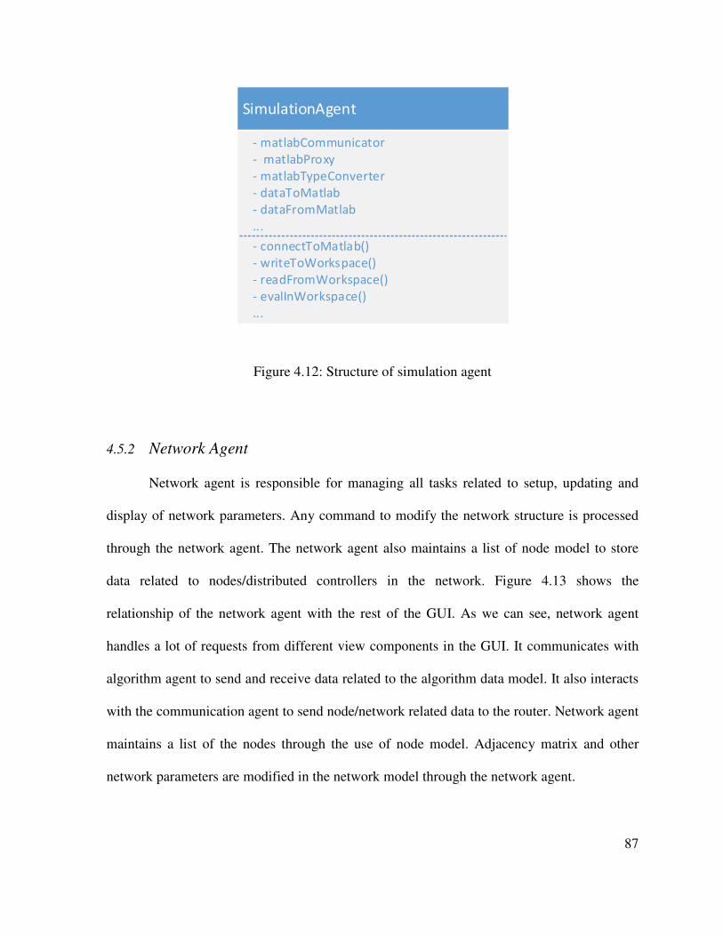
87

SimulationAgent

- matlabCommunicator

- matlabProxy

- matlabTypeConverter

- dataToMatlab

- dataFromMatlab

...

- connectToMatlab()

- writeToWorkspace()

- readFromWorkspace()

- evalInWorkspace()

...

Figure 4.12: Structure of simulation agent

4.5.2 Network Agent

Network agent is responsible for managing all tasks related to setup, updating and

display of network parameters. Any command to modify the network structure is processed

through the network agent. The network agent also maintains a list of node model to store

data related to nodes/distributed controllers in the network. Figure 4.13 shows the

relationship of the network agent with the rest of the GUI. As we can see, network agent

handles a lot of requests from different view components in the GUI. It communicates with

algorithm agent to send and receive data related to the algorithm data model. It also interacts

with the communication agent to send node/network related data to the router. Network agent

maintains a list of the nodes through the use of node model. Adjacency matrix and other

network parameters are modified in the network model through the network agent.

88

Algorithm

Agent

Network Agent

Command Log

Network Topology

Display Panel

Network

Design Canvas

DC Type Selection

Panel

Distributed Controller

Selection Panel

Communication

Agent

Node Model

Network Model

Menu Bar

Data Logging

Agent

Figure 4.13: Network agent relationship with rest of the GUI

Figure 4.14 shows the class structure of NetworkAgent. It contains a list of nodes and

an instantiation of network model to manage the models. Several functions are defined for

the operation of network agent:

• updateNetwork() – This method updates the network model based on the

actions performed in the view panel. This method is triggered when

network design canvas modifies the network topology or when a new

adjacency matrix is uploaded. It is also triggered when specific network

topology such as ring, star is created through the menu bar. Finally,

loading a saved network will also trigger this function.

• updateNode() – This method updated the number and type of nodes in the

89

network based on addition/deletion of nodes performed in the network

design canvas. This method can also be called when new networks of

specific topology are created from the menu bar. Sometimes, algorithm

agent also triggers this method to update the node parameters when a new

algorithm is selected or the parameters of the algorithm relevant to the

node are modified.

• updateView() – This method is gets the latest network structure and node

list from the network and node models and updates appropriate view

components related to the network/node. The tasks performed by this

method include update the display in network canvas, update the

distributed controller type selection panel, update nodes list in distributed

controller selection panel in display window, update the adjacency matrix

display, and update the command log.

• sendNetworkData() –This method sends the network data to the

communication agent which in turns sends it to the router. The network

data is accesses from the network model. This method is triggered by

algorithm agent when a user presses the refresh or run button in the action

panel.

• sendNodeData() – This method sends node data to the communication

agent. It is triggered similar to sendNetworkData().

• getNode()- This node returns the node data model.

90

• getNetwork – This method returns the network model.

NetworkAgent

- NodeModel <list> nodes

- NetworkModel network

...

- updateNetwork()

- updateNode()

- updateView()

- sendNetworkData()

- sendNodeData()

- getNode()

- getNetwork()

...

Figure 4.14: Structure of network agent

4.5.3 Algorithm Agent

Algorithm agent manages the algorithm data models and works as the middleman

between the rest of GUI and the algorithm data model. Since the GUI is a real-time

monitoring platform, algorithm data is accessed and modified from almost every agent.

Figure 4.14 shows the relationship of algorithm agent to the rest of the Green City GUI. As

we can see every other agent/controller interacts with the algorithm agent.

91

Action Panel

Network

Agent

Display Agent

Algorithm

Agent

Simulation

Agent

Communication

Agent

Algorithm

Data Model

ParameterPanel

Agent

Algorithm

Selection Panel

Command Log

Figure 4.15: Relationship of algorithm agent to the rest of GUI

Figure 4.16 shows the class structure of AlgorithmAgent. As we can see it maintains a

list of all the data models implemented in Green City. Currently Green City supports only

one instance of any data model. The list will be used in the future to concurrently record data

from different runs.

AlgorithmAgent

- ConsensusDataModel <list> consensus

- LFICCDataModel <list> lficc

- TwoLevelICCDataModel <list> tl icc

- SecureICCDataModel <list> sicc

- IWCDataModel <list> iwc

- ...

- getAlgorithmModel()

- updateAlgorithmModel()

- sendAlgorithmUpdates()

- updateDisplayPanel()

- runExperiment()

- runSimulation()

...

Figure 4.16: Structure of algorithm agent

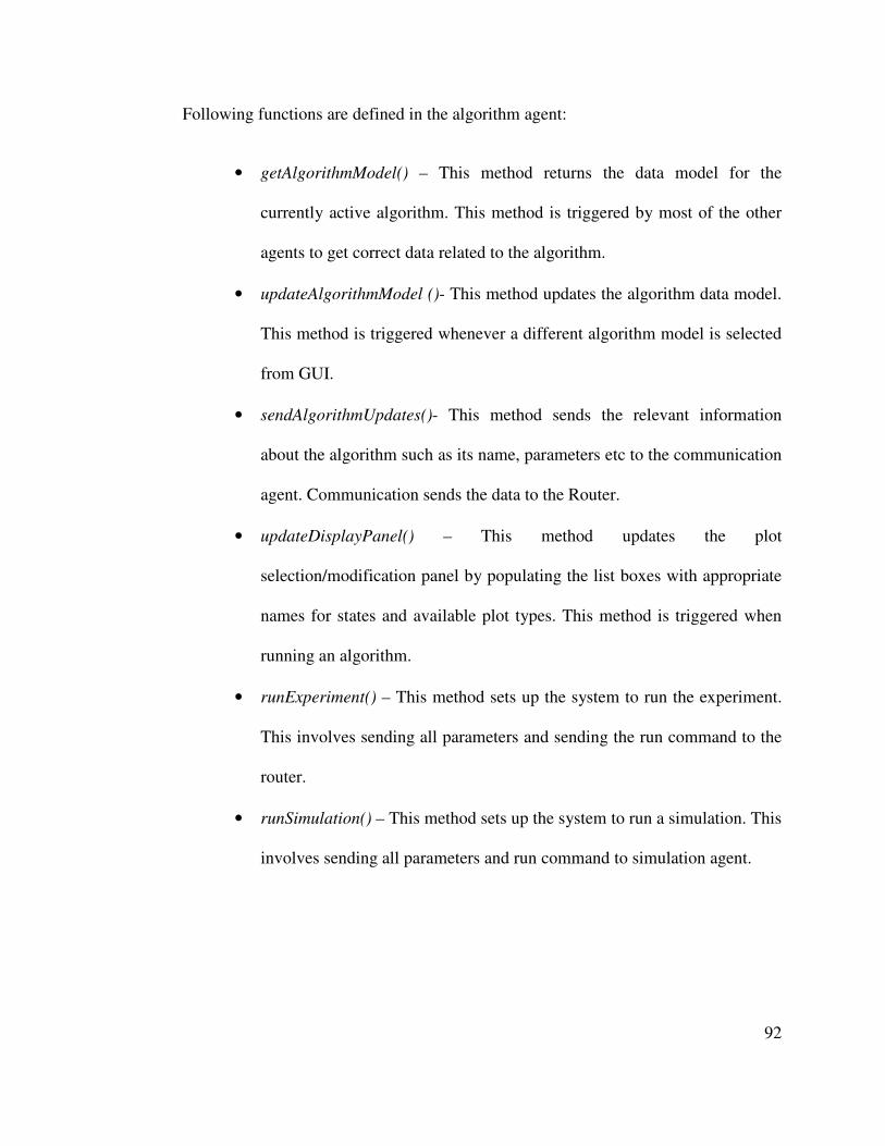
92

Following functions are defined in the algorithm agent:

• getAlgorithmModel() – This method returns the data model for the

currently active algorithm. This method is triggered by most of the other

agents to get correct data related to the algorithm.

• updateAlgorithmModel ()- This method updates the algorithm data model.

This method is triggered whenever a different algorithm model is selected

from GUI.

• sendAlgorithmUpdates()- This method sends the relevant information

about the algorithm such as its name, parameters etc to the communication

agent. Communication sends the data to the Router.

• updateDisplayPanel() – This method updates the plot

selection/modification panel by populating the list boxes with appropriate

names for states and available plot types. This method is triggered when

running an algorithm.

• runExperiment() – This method sets up the system to run the experiment.

This involves sending all parameters and sending the run command to the

router.

• runSimulation() – This method sets up the system to run a simulation. This

involves sending all parameters and run command to simulation agent.

93

4.5.4 Display Agent

Display agent handles the plot window. It is responsible to getting appropriate data

from algorithm model. The data to be retrieved could be any one of the states of single

node/distributed controller or multiple nodes. The process for plotting real-time data as they

are received is different from plotting existing data set. Display agent handles these and

many other scenarios to properly present the data to the operator. Figure 4.17 shows the

relationship of the data agent with the rest of the GUI

Plot Selection/

Modification Panel

Display Agent

Algorithm Agent

Plot Area

Distributed Controller

Selection Panel

Simulation Agent

Menu Bar

Figure 4.17: Relationship of display agent with the rest of the GUI

Figure 4.18 shows the structure of the DisplayAgent class. There are several functions

in the display agent:

• updateNodeList() – This method updates the list of nodes that are selected

in the distributed controller selection panel in display window. The plot

area will plot the state of the nodes that are selected.

94

• setPlotType() – This method determines whether the plot is a real-time

plot or a plot of existing data. It also determines the type of chart to plot.

Currently only XY-plot is available in Green City.

• createXYDataSet() – This method creates and formats the data set to be

plotted. A dataset can contain data series. Data from a single node goes to

a single series.

• createRealTimeDataSet()- This method creates and formats the data set

for plotting in real-time. The real-time window size and plot interval is

defined through this method.

• getNewRTDataPoint() – This method routinely scans the algorithm agent

to see if a new data point is available. If the data point is available, this

method adds the data to the data series.

• getData()- This method requests existing data from algorithm agent for

display.

• createChart() – This method prepares the chart to be displayed in the plot

area. It involves setting the names/units and tick marks in the axes, setting

the title and legend of the plot.

• updateDisplay()- This method updates the plot in the Plot Area.

• updatePlotProperties() – This method updates the properties of the plot

after the plot is already created.

• sendToMatlab() – This method communicates with the simulation agent to

95

send the currently selected data to be plotted in the Matlab window.

DisplayAgent

- double [][] selectedData

- double [] timeValues

- String <list> selectedNodes

- int plotType

- ...

- updateNodeList()

- setPlotType()

- createXYDataSet()

- createRealTimeDataSet()

- getNewRTDataPoint()

- getData()

- createChart()

- updateDisplay()

- updatePlotProperties()

- sendToMatlab()

...

Figure 4.18: Structure of display agent

4.5.5 Parameter Panel Agent

Parameter panel agent updates the changes in the parameter panel and sends relevant

data to the algorithm agent. Figure 4.19 shows the relationship of the parameter panel agent

to the rest of the GUI. Parameter panel takes in the commands from action panel and update

the parameter setup panel by getting the data from parameter panel model and from

algorithm agent. Data from parameter panel model constitute the type and number of inputs

required. Data from algorithm agent include the saved or default values of the inputs.

96

Action Panel

Algorithm

Agent

ParameterPanel

Agent

Parameter

Panel Model

Parameter

Setup Panel

Figure 4.19: Relationship of parameter panel agent with the rest of the GUI

Figure 4.20 shows the structure of the ParameterPanelAgent class. Three main

functions are implemented in the agent:

• initParams()- This method initializes the three types of objects based on

the values of textFields, selectionBoxes and checkBoxes

• updateParams() – Any change in the parameter value in the parameter

panel calls the associated controller to update the values which in turn

calls this method. It updates the parameter values in the model.

• saveParamData() – This method sends the values of the input parameters

to the algorithm agent to update the algorithm model.

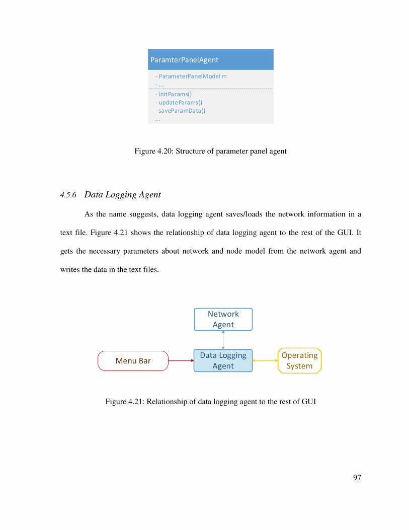
97

ParamterPanelAgent

- ParameterPanelModel m

- ...

- initParams()

- updateParams()

- saveParamData()

...

Figure 4.20: Structure of parameter panel agent

4.5.6 Data Logging Agent

As the name suggests, data logging agent saves/loads the network information in a

text file. Figure 4.21 shows the relationship of data logging agent to the rest of the GUI. It

gets the necessary parameters about network and node model from the network agent and

writes the data in the text files.

Menu Bar

Network

Agent

Data Logging

Agent

Operating

System

Figure 4.21: Relationship of data logging agent to the rest of GUI

98

DataLoggingAgent has a very simple structure as shown in Figure 4.22. It has two

methods to save and load the data.

• saveData() – This method gets the necessary data from network model

and node model and writes it in a text file.

• loadData() – This method reads a text file containing previously saved

network/node data and updates the models through network agent.

DataLoggingAgent

- Filewriter fw

- FileReader fr

- ...

- saveData()

- loadData()

...

Figure 4.22: Structure of data logging agent

4.5.7 Communication Agent

Communication agent relays the message to the Router for further processing and

communication. It uses a TCP socket to write the data from the GUI to the Router and

another socket to read data from the Router. Figure 4.23 shows the relationship of the

communication agent to the rest of the GUI. As we can see, it gets as well as writes

information from both the agents. Note that the Router is an external entity.

99

Network

Agent

Algorithm

Agent

Communication

AgentRouter

Figure 4.23: Relationship of communication agent with the rest of the GUI

Figure 4.24 shows the structure of the CommunicationAgent class. There are two

buffers to store the incoming and outgoing buffer. The port number specifies the address of

the data server which is the Router in this case.

CommunicationAgent

- String <list> incomingBuffer

- String <list> outgoingBuffer

- int portNumber

...

- connect()

- sendData()

- receiveData()

- processData()

...

Figure 4.24: Structure of communication agent

Following methods are defined and implemented in the communication agent:

100

• connect() – This method connects to the Router upon request. The network

agent method triggers this method.

• sendData() - This method sends a data string to the Router. Both

algorithm agent and network agent access this method.

• receiveData() – This method receives the data packets from the Router

and store it in the incoming buffer.

• processData() – This method gets the next data from the incoming buffer

and sends it to appropriate agent for processing.

This completes the discussion on model, view and controller components of the GUI.

The next chapter will discuss the Router.

101

Chapter 5 Router

5.1 Introduction

The Router acts as the middle-man between the graphical user interface and the

distributed controllers. The major functions of the Router are

• Receive setup and control commands from the graphical user interface and

send it to the distributed controllers

• Save and update network related properties such as the network topology,

sampling time for monitoring and make them available to the distributed

controllers upon request,

• Receive and forward messages about state information from distributed

controllers to the graphical user interface for display and monitoring

• Act as a routing agent to exchange messages between two distributed

controllers if the controllers cannot directly communicate with each other

Router program is developed using JAVA programming language. JAVA is used

because both graphical user interface and the distributed controllers are programmed using

JAVA. During the initialization of the network, the router takes the setup commands from the

graphical user interface and sends them to appropriate distributed controller. Once the

experiment is running, the router collects data from each node and sends them to the

graphical user interface for real-time monitoring and control. The router uses TCP/IP

102

protocol to exchange data with the graphical user interface and Bluetooth to send setup

parameters and receive/forward data from/to the distributed controllers. The router contains

two modules that function together to perform these tasks – The communication module and

the network management module.

5.2 The Communication Module

The communication module is a package that is responsible for performing the basic

communication functions of the router. It includes classes and libraries that facilitate sending

or receiving data packets through different communication protocols such as Bluetooth or

TCP/IP and classes to decode and verify the correctness of data packet format. An abstract

class called CommunicationChannel is introduced in the communication module that

contains the standard definition for the sending and receiving data through different

communication mediums. As seen in Figure 5.1, CommunicationChannel class is being

implemented by Bluetooth and TCP_IPSocket classes. Each of these class implements the

three main functions to connect, send and receive data from other communication nodes.

5.2.1 Bluetooth Class

Bluetooth class implements the functions to enable communication with the LEGO

Mindstorm microcontrollers. In-built functions from LeJOS library along with some

modifications are used in the Bluetooth class. The Bluetooth class also contains the table of

message type as shown in Table 3-I. In addition to the message types, the Bluetooth type also

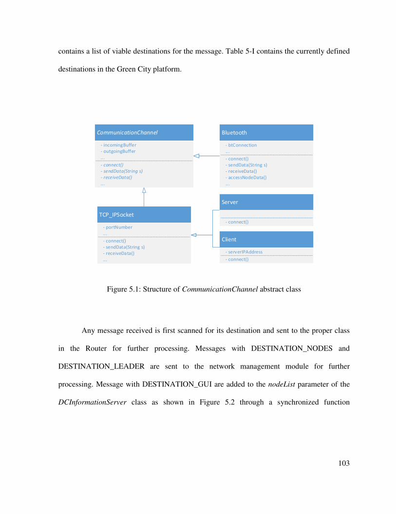
103

contains a list of viable destinations for the message. Table 5-I contains the currently defined

destinations in the Green City platform.


- incomingBuffer

- outgoingBuffer

...

- connect()


- receiveData()

...

Bluetooth

- btConnection

...

- connect()


- receiveData()

- accessNodeData()

...

TCP_IPSocket

- portNumber

...

- connect()


- receiveData()

...

Server

- connect()

Client

- serverIPAddress

- connect()

Figure 5.1: Structure of CommunicationChannel abstract class

Any message received is first scanned for its destination and sent to the proper class

in the Router for further processing. Messages with DESTINATION_NODES and

DESTINATION_LEADER are sent to the network management module for further

processing. Message with DESTINATION_GUI are added to the nodeList parameter of the

DCInformationServer class as shown in Figure 5.2 through a synchronized function

104

accessNodeData(). Messages from node that are sent just to create background traffic have

DESTINATION_NONE and are discarded once received.

Table 5-I: List of valid destination points for data packets in Router

Destination ID

DESTINATION_NODES 0

DESTINATION_GUI 1

DESTINATION_LEADER 2

DESTINATION_NONE 3

Bluetooth class also handles the priority of the data packet being received. Currently

any data packet can have the priorities listed in Table 5-II. Data packets with high priority are

added at the beginning and with low priority are at the end of the datapacket buffers (such as

the nodeList).

Table 5-II: Priorities defined in the Bluetooth Class

PRIORITY_LOW 0

PRIORITY_HIGH 1

105

5.2.2 TCP_IPSocket Class

TCP_IPSocket class implements the functions for sending and receiving data through

the TCP/IP protocol. This class is used in sending and receiving messages to the graphical

user interface. Two types of TCP/IP socket communication classes are defined – the server

and the client. These two classes are almost the same expect that a client needs an IP address

of the server it is going to connect to. Usually a server receives a request from the client and

replies to the request and the client sends a request and gets the server’s reply. Two servers

are defined in Router to handle the communication from the graphical user interface (GUI) as

shown in Figure 5.2.

NetworkSetupServer handles all the setup and control related data packets that are

received from the GUI. This server keeps on listening to the messages received from the

GUI. Once a message is received the server executes a parseCommand() function.

parseCommand() function is implemented through the use of CommandParser class.

106

Server

- connect()

DCInformationServer

- nodeDataList

- samplingInterval

- ...

- accessNodeData()

- ...

NetworkSetupServer

- commandParser

- ...

- waitForGUICommand()

- parseCommand()

- ...

CommandParser

- commandBuffer

- validCommandsList

- validParameters

- validModifiers

- validExpressions

- ...

- checkSyntax()

- checkLogic()

- updateCommandBuffer()

1

CommandBuffer

- commandList

- parameterList

- modifierList

- expressionsList

1

Figure 5.2: GUI related servers in Router

CommandParser class contains the definitions of all the valid commands in the Green

City architecture. It parses the command and checks its syntactic and logical validity. A

command is in the form

COMMAND <parameter> modifier1 (expression1)…modifier2…

There are four components to a command:

• Command: This field is used by the Router to determine the type of

command sent from the GUI, for example whether it is a algorithm setup

related command or a network setup related command etc.

107

• Parameter: This field is used by the Router to discern what needs to be

done (e.g.: establishing Bluetooth connectivity for a particular node)

• Modifier: These fields are used to denote any special characteristics that

the Router needs to know about the command.

• Expression: These fields follow modifiers and are the values that are

associated with a particular modifier.

The parsing algorithm is broken into two main components: syntax checking and

logic checking. Syntax checking is accomplished by checking the validity of a command’s

directives, command tag, parameter tag, and modifier/expression tags. This information is

checked against a list of valid options. The algorithm was defined in such a way as to be

easily modifiable; that is to say, the syntax checking can quickly be expanded to incorporate

new commands, modifiers, parameters, and/or directives. In addition to the syntax checker,

there is also a logic checker for each command. The logic checker is used as a final means to

verify the correctness of a command by eliminating commands that are syntactically correct,

but logically wrong. Logically and syntactically valid commands are then stored as a list in

the CommandBuffer class which is then accessed by the Network management module for

further processing.

5.3 The Network Management Module

The major functions of the network management module are

• Get valid commands from the command buffer and send it to appropriate

108

nodes

• Maintain a list of online nodes and notify the GUI

• Create and maintain a communication channel each for receiving data

from the nodes and sending data to the nodes

• Store common network related parameters such as the topology, sample

time, and parameters specific to different distributed algorithms such as

over all power demand, step-size (as in the case of Incremental Cost

Consensus (ICC) algorithm), reputation/similarity threshold (as in the case

of secure ICC) etc

In order to perform these functions, the network management module has three

classes as shown in Figure 5.3.

5.3.1 GUICommandHandler Class

GUICommandHandler class maintains a copy of the CommandBuffer class and

accesses valid commands from the command lists. It then proceeds to check the type of

command. The command can either be a network wide command such as the topology

change, sampling time change, algorithm parameter initialization for the entire network, etc

or it can be a node related command such as connect to a particular node, update specific

node parameter etc. GUICommandHandler identifies the command by the keywords in the

command and executes either processNodeRequest() or processNetworkRequest() command

109

to complete the task required by the command. This class maintains a static instance of

NetworkAgent class.

GUICommandHandler

- networkAgent

- commandBuffer

- getCommand()

- processNodeRequest()

- processNetworkRequest()

NetworkAgent

- nodeList

- adjacencyMatrix

-...

- connectNode()

- setNetworkParameters()

- setTopology()

- sendGlobalData()

- runExperiment()

Node

- btConnection

- ...

- establishConnection()

- startComm()

- stopComm()

- disconnect()

- runAlgorithm()

- stopAlgorithm()

- getData()

- sendData()

0..*

CommandBuffer

- commandList

- parameterList

- modifierList

- expressionsList

1

1

Figure 5.3: Class structure of the network management module

5.3.2 NetworkAgent Class

Network Agent class is perhaps the most important class in the Router. It carries out

most of the task related to the setup and control of the distributed controllers. It maintains a

list of Nodes. A new node is added to the list for every node that Router is connected to. As

110

such Router maintains a virtual copy of the every active node in the network. Since Network

agent is the only class that maintains the node list, all the commands to the node have to be

accessed through the NetworkAgent. The main functions in the NetworkAgent created to

setup and control the nodes are briefly described below

• connectNode() – this method scans through the list of available nodes and

connects to them. It is usually executed at the beginning of an experiment.

The operator can also execute this function if new nodes are being added

to the system.

• setNetworkParameters() – as the name implies, this function sets up the

parameters related to the network. Such parameters could be common to

all the algorithms such as topology, sampling time or specific to some

algorithms.

• setTopology() – this function sets up the topology of the network by

maintaining an adjacency matrix of the network nodes and the connections

between them. The adjacency matrix can be updated at any instance by the

operator upon which this function is executed. It also sends the related

data about the adjacency matrix to each individual nodes in the network

• sendGlobalData() – this function sends the global data specific to each

algorithm to the nodes/distributed controllers in the network

• runExperiment() – this is a thread that runs when a new experiment is

being run by the operator. It stops upon reaching the stopping condition

111

for the experiment. Stopping condition can either be defined as a time

limit or a limit in the number of iterations. The operator can also force

stop an experiment

5.3.3 Node Class

The Node class is a virtual copy of the distributed controller in the network. Through

the node class, the Network Agent can send and receive data to the distributed controller to

which the node is associated to. Node maintains na individual Bluetooth connection to the

distributed controller that it is associated to. Primary functions such as sending data, getting

data, connecting to the distributed controller, disconnecting from the distributed controller,

running or stopping an experiment on a distributed controller is done through the Node Class.

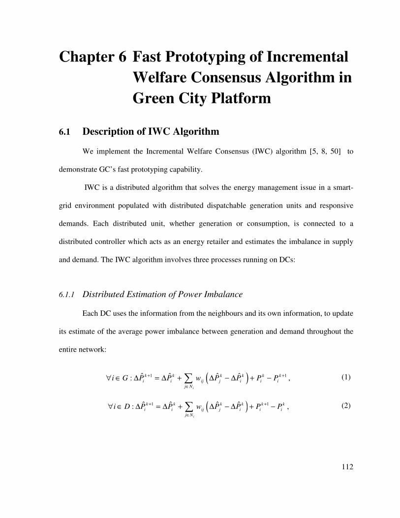
112

Chapter 6 Fast Prototyping of Incremental

Welfare Consensus Algorithm in

Green City Platform

6.1 Description of IWC Algorithm

We implement the Incremental Welfare Consensus (IWC) algorithm [5, 8, 50] to

demonstrate GC’s fast prototyping capability.

IWC is a distributed algorithm that solves the energy management issue in a smart-

grid environment populated with distributed dispatchable generation units and responsive

demands. Each distributed unit, whether generation or consumption, is connected to a

distributed controller which acts as an energy retailer and estimates the imbalance in supply

and demand. The IWC algorithm involves three processes running on DCs:

6.1.1 Distributed Estimation of Power Imbalance

Each DC uses the information from the neighbours and its own information, to update

its estimate of the average power imbalance between generation and demand throughout the

entire network:

( )1 1ˆ ˆ ˆ ˆ: ,i

k k k k k k

i i ij j i i i

j N

i G P P w P P P P+ +

∈

∀ ∈ ∆ = ∆ + ∆ − ∆ + −∑ (1)

( )1 1ˆ ˆ ˆ ˆ: ,i

k k k k k k

i i ij j i i i

j N

i D P P w P P P P+ +

∈

∀ ∈ ∆ = ∆ + ∆ − ∆ + −∑ (2)

113

where ˆ k

iP∆ is the estimate of the i-th unit from the value of the average power imbalance at

the k-th iteration, Ni is the set of neighbors of node i, wij = wji is the connectivity strength

between node i and node j and k

iP is the generated/consumed power of the i-th unit at the k-th

iteration. The set of indices of demand units is denoted by D, and the set of indices of

generation units is denoted by G.

6.1.2 Local Price Update

Based on the estimation of power imbalance between supply and demand, the local

price is updated at each distributed unit:

( )1 ˆ: ,i

k k k k k

i i ij j i i

j N

i G D w Pλ λ λ λ η+

∈

∀ ∈ ∪ = + − + ∆∑ (3)

where k

iλ is the price of energy of the i-th unit at the k-th iteration and η is the updating step-

size.

6.1.3 Power Regulation

Based on the updated price of energy, each unit updates the amount of power

consumption/generation to maximize its profit (or equivalently minimize its cost):

( ),max

1

0: arg min ( ) ,

i i

k k

i i i i iP P

i D P P U Pλ+

≤ ≤∀ ∈ = −

( ),min ,max

1: arg min ( ) ,i i i

k k

i i i i iP P P

i G P C P Pλ+

≤ ≤∀ ∈ = −

(4)

114

where Ui(.) and Ci(.) are the utility and cost functions of the i-th respectively and Pi,min and

Pi,max represent the minimum and maximum bounds for power consumption/generation. The

utility function for the i-th consumer unit is defined as:

2

2

/ 2( ) ,

/ 4 / 2

i i i i i i i

i i

i i i i i

P P PU P

P

ω α ω α

ω α ω α

− ≤=

≥ (5)

where ω and α are positive values differentiating the consumers. The cost function for the i-

th generation unit is considered as:

2( ) ,i i i i i i i

C P a P b P c= + + (6)

where ai , bi and ci are predetermined constants.

6.2 Fast Prototyping of IWC Algorithm

Figure 6.1 shows the class diagram of the functional agent in the control layer.

Functional agent performs tasks related to setting up, starting and stopping an algorithm. An

abstract class called DistributedAlgorithm serves as a template to create/add new distributed

algorithm into the GC platform. This abstract class contains the implementation of

updateLocalData() that gets the data from the local sensor data buffer and definition of three

other functions: updateParameters(), updateNeighborData() and compute(). In order to

successfully implement IWC algorithm in GC, the developer has to:

• Create an IncrementalWelfare object that inherits the properties and

methods of the DistributedAlgorithm class, and

• Implement the following three methods:

115

• updateParameters()– initialize/update parameters related to the algorithm.

Parameters are set/modified through the GUI by the operator

• updateNeighborData()– get updated data from neighbor data buffer at

every iteration.

• compute()– perform the algorithm tasks (for e.g. in IWC, implement the

distributed observer, price regulator and power regulator) and store the

data in control decisions buffer with appropriate data id.

FunctionalAgent

- DistributedAlgorithm d

-setUpAlgorithm(String name)- startAlgorithm()- stopAlgorithm()

DistributedAlgorithm

- String algorithmName- Arraylist localData, neighborData, controlData

- updateLocalData()- updateParameters(String s)


- compute()

IncrementalWelfare

1

Consensus ...

Figure 6.1: Class diagram of the functional agent and the distributed algorithm class

Figure 6.2 shows the block diagram showing different functions that are implemented

for fast prototyping of IWC algorithm.

116

Price

Regulator

Distributed

Observer

Generation/

Demand Unit

Neighbor

Data

Utility/Cost Function

Parameters

Generated/

Consumed Power

Energy Price at

Neighbors

To

Neighbors

Power

Regulator

Energy Price

Compute ()

Estimate of Power Imbalance

updateNeighbor

Data()

updateLocalData()

updateParameters()

Data

from

GUI

Figure 6.2: Different functions implemented by IWC algorithm

6.3 Experimental Results

6.3.1 Experimental Setup

A Garver Power Network [51] as shown in Figure 6.3 is used to demonstrate the

implementation results under different scenarios. The network is a 5-bus system that consists

of 2 generation units (CG1, CG2) and 5 demand units (LD1, LD2, LD3, LD4 and LD5).

Three (LD2, LD4, and LD5) out of the five demand units are responsive demands and the

rest (LD1 and LD3) are constant demands. Each unit is controlled using a DC.

117

Figure 6.3: Distributed controllers in a Garver power network

The parameters for the utility/cost functions for each unit are provided in Table 6-I.

The rest of this section discusses the results of IWC algorithm at different case studies to

showcase the features of the GC platform. All of these case studies use the parameters from

Table 6-I. The initial conditions for the consensus values were set to zero, the step-size, η,

was set to 0.005, and the experiments were run for 40s unless otherwise specified. The global

optimal price calculated for this scenario using centralized quadratic programming was 8.011

cents/KWH. The analysis of the behavior of the algorithm under different scenarios is not a

part of this paper.

118

Table 6-I: Generation/Demand Unit Parameters

Node Demand ω α Pmin(kW) Pmax(kW)

2 LD1 - - 20 20

3 LD2 15 0.0750 0 100

4 LD3 - - 30 30

6 LD4 12 0.1200 0 50

7 LD5 20 0.2000 0 50

Generation a b Pmin(kW) Pmax(kW)

1 CG1 0.0080 7 0 100

5 CG2 0.0096 6.4 0 80

6.3.2 Case Study 1: Reconfigurability

Note that DCs are configured as generator, non-responsive load or responsive load by

simply sending a configuration command to the DC from the GUI. Upon receiving the

configuration command and type, the DC configures itself by instantiating appropriate

Nodetype through the use of configuration agent. As shown in Figure 6.4, configuration

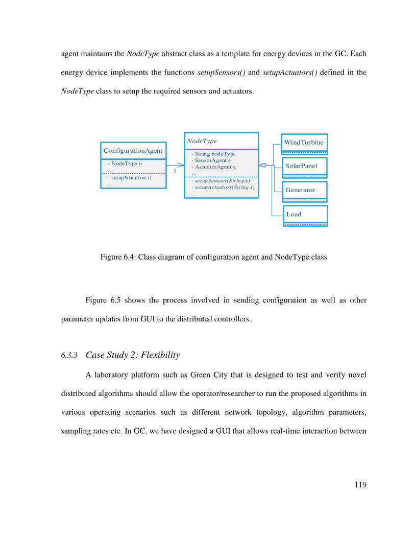
119

agent maintains the NodeType abstract class as a template for energy devices in the GC. Each

energy device implements the functions setupSensors() and setupActuators() defined in the

NodeType class to setup the required sensors and actuators.

ConfigurationAgent

- NodeType n

...

- setupNode(int i)

...

NodeType

- String nodeType

- SensorAgent s

- ActuatorAgent a

...



...

WindTurbine

SolarPanel1

Generator

Load

Figure 6.4: Class diagram of configuration agent and NodeType class

Figure 6.5 shows the process involved in sending configuration as well as other

parameter updates from GUI to the distributed controllers.

6.3.3 Case Study 2: Flexibility

A laboratory platform such as Green City that is designed to test and verify novel

distributed algorithms should allow the operator/researcher to run the proposed algorithms in

various operating scenarios such as different network topology, algorithm parameters,

sampling rates etc. In GC, we have designed a GUI that allows real-time interaction between

120

the operator and the power network. Different network and algorithm parameters can be

changed during the runtime using the set-up window.

Operator Change ParametersSend Update

Request

Send Data to DCs

Receive and Decode DataPacket

Notify

Configuration Agent

Set Node Type

Update Sensors/

Actuators

Configuration

Parameter?

Algorithm

Parameter?

Notify Functional

Agent

Verify Parameters

Update Parameters

GUI

Router

DC

Yes

No

Yes

Notify Routing

Agent

Verify Parameters

Update Routing

Table

Network

Parameter?

Disturbance

Parameter?

Notify Disturbance

Agent

Verify Parameters

Update Noise/Delay

Yes

No

Yes

No

Figure 6.5: Process involved in changing parameters in Green City

6.3.3.1 Case Study 2a - Network Topology

Figure 6.6 shows the snapshots of four common network topologies created using the

network design canvas of the GC platform. The Garver power based topology was created by

creating one-to-one correspondence between the power lines and the communication links in

121

the Garver Power Network. The green nodes represent the controllers for generation units

and the blue nodes represent the controllers for demand units. The blue dotted lines represent

communication link between two DCs. GC platform allows the flexibility to add/remove

nodes and communication links to study the effect of network topology on the convergence

of IWC.

Figure 6.6: Snapshot of network topologies (left to right: (Top) Chain, Star Fully Connected

and (bottom) Garver Power based) created in Green City

Figure 6.7 shows the evolution of price of the power for different units. We can

observe that the convergence time is the slowest (~32s) in the chain topology and fastest

(~20s) in fully connected topology. The dotted line represents the global optimal point for

price. The difference in price during the transient phase is the largest for star topology.

Figure 6.7: Evolution of price for different network topologies (From left to Right

Chain, Star; Bottom: Fully Connected, Garver Power based)


The difference in price during the transient phase is the largest for star topology.

: Evolution of price for different network topologies (From left to Right


122


The difference in price during the transient phase is the largest for star topology.

: Evolution of price for different network topologies (From left to Right - Top:


123

6.3.3.2 Case Study 2b - Algorithm Parameters

A fast prototyping platform should show allow easy integration of changes in the

algorithm. Green city supports fast prototyping by allowing the user to change existing

parameters on the run. In this case study, we demonstrate this feature by running IWC

algorithm under four different step-size (η) values. Figure 6.8 shows performance of IWC at

η = 0.001, 0.005, 0.01, and 0.1 respectively. Results show that step-size directly affects the

convergence of the IWC algorithm. The algorithm converges the slowest (~100s) when step-

size is smallest. High step-size implies a faster convergence up to a certain point. When step-

size is too high (0.1 in this case) IWC becomes unstable.

Figure 6.8: Evolution of price at different values of step size,

– η = 0.005;

6.3.4 Case Study 3: Performance Study under Communication Constraints

Testing distributed control algorithms under communication constraints is very

important for the study of their convergence behavior. In this case study, we show that using

ice at different values of step size, η (Top: Left –

= 0.005; Bottom: Left – η = 0.01, Right – η = 0.1)

Case Study 3: Performance Study under Communication Constraints


f their convergence behavior. In this case study, we show that using

124

η = 0.001, Right

Case Study 3: Performance Study under Communication Constraints


f their convergence behavior. In this case study, we show that using

the GC platform we were able to observe the behavior of the IWC algorithm under

communication delay and noise.

6.3.4.1 Case Study 3a - Communication Delay

Two scenarios were considered for testing under delay, where network wide constant

delay of 100ms (delay less than sampling time) and 600ms (delay greater than sampling

time) were added to the system. Green city generates dela

based on the current network load.

delay conditions. When the delay is less than the sampling time, the algorithm converges

the global optimum; however, algorithm converges to a sub

greater than the sampling time. In

converges to zero.

Figure 6.9: Evolution of price at delay=100ms (Left) & delay=600ms (Right)


communication delay and noise. The communication sampling time was set to be 500ms.

Communication Delay



time) were added to the system. Green city generates delay by injecting background traffic

based on the current network load. Figure 6.9 shows the consensus variable price under two

delay conditions. When the delay is less than the sampling time, the algorithm converges

the global optimum; however, algorithm converges to a sub-optimal point when the delay is

greater than the sampling time. In Figure 6.10, we see that the power imbalance in both cases

: Evolution of price at delay=100ms (Left) & delay=600ms (Right)

125


he communication sampling time was set to be 500ms.



y by injecting background traffic

shows the consensus variable price under two

delay conditions. When the delay is less than the sampling time, the algorithm converges to

optimal point when the delay is

the power imbalance in both cases

: Evolution of price at delay=100ms (Left) & delay=600ms (Right)

Figure 6.10: Power imbalance at delay=100ms (Left) and delay = 600ms (Right)

6.3.4.2 Case Study 3b - Communication Noise

Similarly, two scenarios were considered for testing under noise. In the first scenario,

Gaussian noise with mean 0.01 and variance of 0.001 was injected to the consensus variables

price and power imbalance. In the second

0.01. We can observe from

Furthermore, as we can see in

There is a negative power imbalance implying that the demand is greater than the supply.

This imbalance will cause the price to keep on increasing. These observations suggest that

the IWC is very sensitive to noise.

: Power imbalance at delay=100ms (Left) and delay = 600ms (Right)

Communication Noise



price and power imbalance. In the second scenario the mean was set to 0.1 with a variance of

0.01. We can observe from Figure 6.11 that the price fails to converge in both cases.

Furthermore, as we can see in Figure 6.12, power imbalance also does not converge to 0.



ive to noise.

126

: Power imbalance at delay=100ms (Left) and delay = 600ms (Right)



scenario the mean was set to 0.1 with a variance of

that the price fails to converge in both cases.

power imbalance also does not converge to 0.



Figure 6.11: Evolution of price when adding Gaussian noise with 0.01 mean and 0.001

variance (Left) and with 0.1 mean and 0.01 variance (Right)

Figure 6.12: Evolution of power imbalance estimations when adding Gaussian noise with

0.01 mean and 0.001 variance (Left) and with 0.1 mean and 0.01 variance (Right)

: Evolution of price when adding Gaussian noise with 0.01 mean and 0.001


: Evolution of power imbalance estimations when adding Gaussian noise with


127

: Evolution of price when adding Gaussian noise with 0.01 mean and 0.001


: Evolution of power imbalance estimations when adding Gaussian noise with


128

6.3.5 Case Study 4: Real-time Monitoring under Dynamic Scenarios

This final case study showcases the real-time monitoring capability of the green city

platform. In this case, the IWC algorithm is run in Garver power network based topology

with the initial conditions shown in Table 6-I at time t = 0s. Different events listed below

were introduced while the IWC was running. (E1 represents event 1, E2 – event 2 and so

on...)

• E1: At t =5s, CG2 gets disconnected from communication network

• E2: At t = 15s, the maximum power limit for LD5 increases from 50 to 100

• E3: At t = 25s, LD4 gets disconnected from the communication network.

• E4: At t =30s, maximum power limit for LD4 increases to 150 even though it

is not connected to the rest of the network.

• E5: At t =40s, LD4 and CG2 are both back online

• E6: At t = 50s, the maximum power constraint for LD4 and LD5 goes back to

50.

Figure 6.13 shows the evolution of the price in the IWC algorithm along this dynamic

scenario. The disconnection of CG2 can be observed in the plot where the price of CG2 as

well as LD3 deviates from the rest of the network. When the maximum power limit for LD5

is increased at E2, the rest of the controllers which are still intact in the original network

respond to the changes in the network by increasing the price due to an increase in demand.

After LD4 is disconnected at E3 and its maximum power limit is increased at E4, we can see

that LD4 itself is responding to the change in its parameters, however the rest of the network

is unresponsive to this change because of

responds to this change when LD4, CG2 and LD3 come online at

conditions become similar to the initial condition, the price starts to converge to the global

optimum point. In addition

flexibility of the green city platform in creating dynamic scenarios such as link failure, node

failure, parameter changes etc.

Figure 6.13: Real-


is unresponsive to this change because of LD4 being offline. The network immediately

responds to this change when LD4, CG2 and LD3 come online at E5. Finally at


. In addition to real-time monitoring, this case study also showcases the


failure, parameter changes etc.

-time monitoring in green city under dynamic scenario

129


LD4 being offline. The network immediately

. Finally at E6, since all


time monitoring, this case study also showcases the


time monitoring in green city under dynamic scenario

Using the green city platform we can also monitor other parameters of interest for the

IWC algorithm. For example

6.15 shows the demand and generation for different distributed controllers.

Figure 6.14: Evolution of power imbalance (Left) and welfare (Right)


IWC algorithm. For example Figure 6.14 shows the power imbalance and wel

shows the demand and generation for different distributed controllers.

: Evolution of power imbalance (Left) and welfare (Right)

130


shows the power imbalance and welfare, and Figure

: Evolution of power imbalance (Left) and welfare (Right)

Figure 6.15: Evolution of demand (Left) and generation (Right)

: Evolution of demand (Left) and generation (Right)

131

: Evolution of demand (Left) and generation (Right)

132

Chapter 7 Testing Distributed Energy

Management Algorithms under

Security Constraints in Green

City

This chapter will demonstrate the use of Green City platform to evaluate a distributed

control algorithm under security constraints. Two algorithms (i) The Leader-Follower

Incremental Cost Consensus (LFICC) algorithm[5] and (ii) The Secured LFICC algorithm

[46] will be tested under different kinds of security attacks.

7.1 Implementation Details

7.1.1 Leader-Follower Incremental Cost Consensus Algorithm

The leader-follower incremental cost consensus (LFICC) algorithm is a consensus

[52] based distributed algorithm for energy distribution problem (EDP). The objective of

solving the EDP is to minimize the total cost of operations. Traditionally, all of the generator

parameters have to be sent to the control centre. The control centre calculates the optimal

system operation point based on the information acquired from the entire system. By using

the consensus algorithm and selecting the incremental cost (IC) as the consensus variable,

the EDP can be solved in a distributed manner. The distributed controller (embedded in

each generation unit) will update its own IC based on its neighbours’ ICs. In addition, a

“leader unit” has to be selected, which will control whether to increase or decrease the

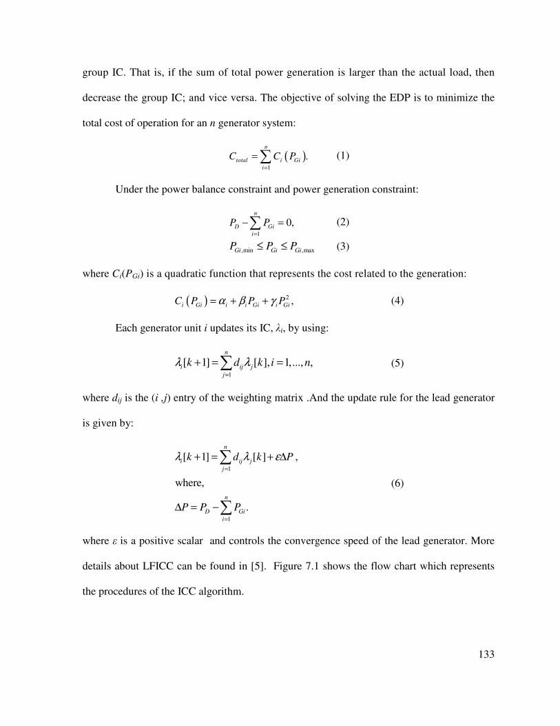
133

group IC. That is, if the sum of total power generation is larger than the actual load, then

decrease the group IC; and vice versa. The objective of solving the EDP is to minimize the

total cost of operation for an n generator system:

( )1

.n

total i Gi

i

C C P=

=∑ (1)

Under the power balance constraint and power generation constraint:

1

0,n

D Gi

i

P P=

− =∑ (2)

,min ,maxGi Gi GiP P P≤ ≤ (3)

where Ci(PGi) is a quadratic function that represents the cost related to the generation:

( ) 2 ,i Gi i i Gi i GiC P P Pα β γ= + + (4)

Each generator unit i updates its IC, λi, by using:

1

[ 1] [ ], 1,..., ,n

i ij j

j

k d k i nλ λ=

+ = =∑ (5)

where dij is the (i ,j) entry of the weighting matrix .And the update rule for the lead generator

is given by:

1

1

[ 1] [ ] ,

where,

.

n

i ij j

j

n

D Gi

i

k d k P

P P P

λ λ ε=

=

+ = + ∆

∆ = −

∑

∑

(6)

where ε is a positive scalar and controls the convergence speed of the lead generator. More

details about LFICC can be found in [5]. Figure 7.1 shows the flow chart which represents

the procedures of the ICC algorithm.

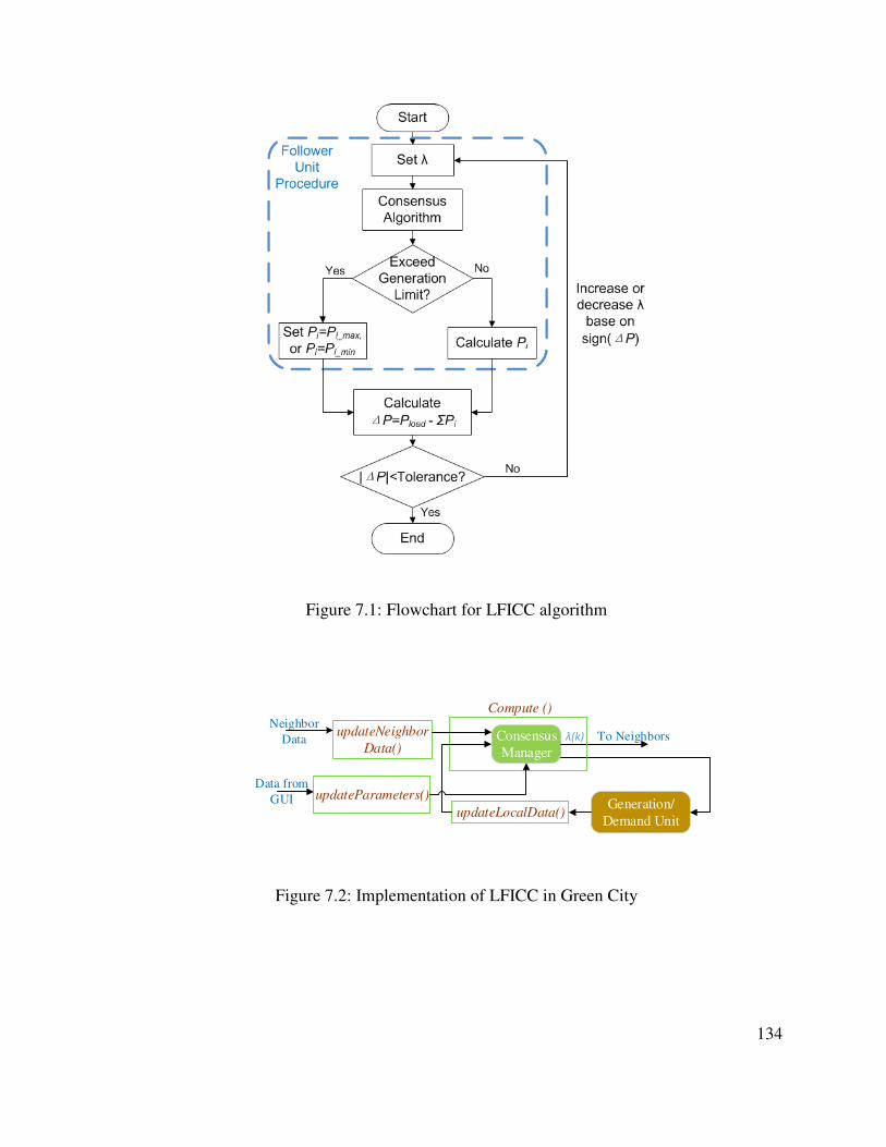
134

Figure 7.1: Flowchart for LFICC algorithm

Generation/Demand Unit

Neighbor

Data To NeighborsConsensus Manager

λ(k)

Compute ()

updateNeighbor

Data()

updateLocalData()

updateParameters()Data from

GUI

Figure 7.2: Implementation of LFICC in Green City

135

7.1.2 Secured Distributed Control Algorithm

The secure distributed control methodology embeds the following four phases into

each iteration of the consensus computation (i.e., reference state update) process: (1) Detect

the neighbours’ misbehaviours relying only on each distributed controller’s local

observations through Neighbourhood Monitor; (2) Adjust the consensus computation weights

according to neighbours’ reputation values via Local Reputation Manager; (3) Identify and

isolate the compromised distributed controller; and (4) Use the adjusted consensus

computation weights to calculate the updated reference state to ensure the convergence of the

well-behaving distributed controllers. The detailed description of each phase is given below.

7.1.2.1 Neighbourhood Monitor

In this Neighbourhood Monitor, the distributed controller carries out a real-time

anomaly detection mechanism for all its neighbours by redundantly calculating and storing

its neighbour’s j’s reference state rj and comparing it with the state value λj received from the

neighbour j in time step k. If rj[k] = λj[k], the neighbour is normal; if rj[k]≠λj[k], the

neighbour has potential anomaly.

[ 1] 1, [ ] [ ] 0[ ] ,

[ 1], [ ] [ ] 0

ij j j

ij

ij j j

G k r k kG k

G k r k k

λ

λ

− + − ==

− − ≠ (7)

where Gij is the total number of verifiably correct states of neighbour distributed controller j

up to time-step k monitored by distributed controller i.

136

7.1.2.2 Local Reputation Manager

The Local Reputation Manager is an onboard system that updates the reputation

values of the neighbour distributed controller using Bayesian reputation function and records

them in its local reputation table.

[ ] 1[ ] ,

2

ij

ij

G krep k

k

+=

+ (8)

where repij is the reputation value of neighbour distributed controller j up to time-step k in

distributed controller i’s Local Reputation Manager.

In the Local Reputation Manager, a misbehaviour or good behaviour as the result of

the Neighbourhood Monitor is used to update the neighbour robot’s reputation value. If the

reputation value falls below a certain level (malicious threshold repM), the neighbour robot is

identified as a compromised robot and will be isolated.

7.1.2.3 Adaptive Consensus Computation

In order to embed the above security mechanisms in the consensus computation

process, a method to adaptively update the consensus computation weights dij, which is the

(i, j) entry of the row-stochastic matrix D, based on the reputation values from the Local

Reputation Manager. The method is shown below:

1

[ ] [ ] [ ]n

ij ij ij

j

d k rep k rep k=

= ∑ . (9)

Thus, the robot reference state update rule in the consensus manager is

correspondingly changed to:

137

1

[ 1] [ ] [ ], 1,..., ,n

i ij j

j

k d k k i nλ λ=

+ = =∑ (10)

By implementing this method, a feedback loop from the output of the security

mechanism to the input of the distributed controller (consensus manager) is built, as shown in

Figure 7.3. More details about Secure Distributed Control algorithm is given in [46].

Reputation manager

Neighborhood Monitor

Generation/Demand Unit

Neighbor

Data

Rep threshold,

parameters

Generated/

Consumed Power

To

Neighbors

Consensus Manager λ(k)

Compute ()

G(k) d(k)r(k)

updateNeighbor

Data()

updateLocalData()

updateParameters()

Data

from

GUI

λ(k)

r(k)

Figure 7.3: Implementation of Secure distributed control methodology in Green City

7.1.3 Attack Models

A distributed controller under malicious cyber attack is called a misbehaving

controller. The misbehaving controller dynamics can be defined as:

1

[ 1] [ ] [ ],n

i ij j M M

j

k d k B u kλ λ=

+ = +∑ (11)

where uM is the malicious cyber attack that is modelled as an exogenous input to the

consensus manager.

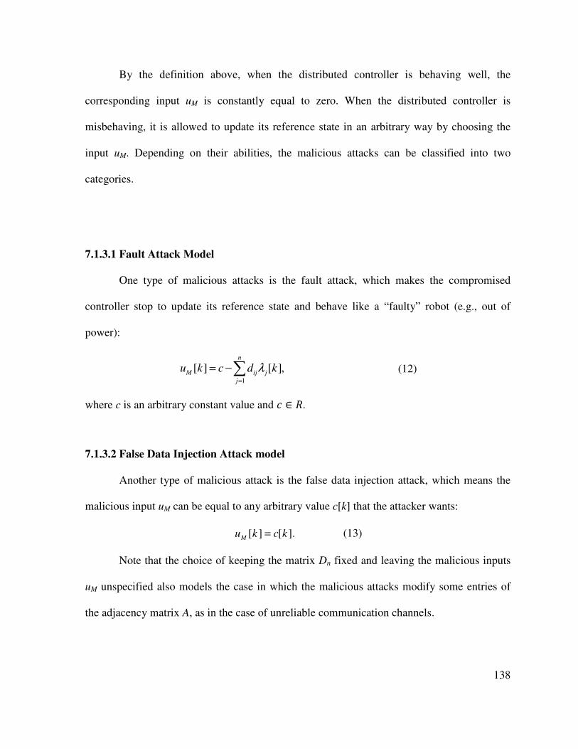
138

By the definition above, when the distributed controller is behaving well, the

corresponding input uM is constantly equal to zero. When the distributed controller is

misbehaving, it is allowed to update its reference state in an arbitrary way by choosing the

input uM. Depending on their abilities, the malicious attacks can be classified into two

categories.

7.1.3.1 Fault Attack Model

One type of malicious attacks is the fault attack, which makes the compromised

controller stop to update its reference state and behave like a “faulty” robot (e.g., out of

power):

1

[ ] [ ],n

M ij j

j

u k c d kλ=

= −∑ (12)

where c is an arbitrary constant value and ∈ .

7.1.3.2 False Data Injection Attack model

Another type of malicious attack is the false data injection attack, which means the

malicious input uM can be equal to any arbitrary value c[k] that the attacker wants:

[ ] [ ].Mu k c k= (13)

Note that the choice of keeping the matrix Dn fixed and leaving the malicious inputs

uM unspecified also models the case in which the malicious attacks modify some entries of

the adjacency matrix A, as in the case of unreliable communication channels.

139

7.2 Experiments and Results

7.2.1 Experimental Setup

Figure 7.4 shows the network topology used for demonstrating the effect of security

attacks on the network. The network consists of five generation units (CG0, CG1, CG2, CG3,

and CG4). The red node denotes the malicious node.

Figure 7.4: Network topology used for case studies

Table 7-I and Table 7-II show the parameters used for the experiments for the

generation units and the network respectively.

140

Table 7-I: Parameters of the generation units for LFICC

Unit αi βi γi

CG0 561 7.92 0.001562

CG1 310 7.85 0.00194

CG2 78 7.97 0.00482

CG3 561 7.92 0.001562

CG4 310 7.85 0.00194

Table 7-II: Parameters of the Power Network

Parameters Value

PD , (MWH) 500

ε 5e-4

Leader CG0

λ(0) 5

141

Table 7-III shows the values of the additional parameters required by the Secured

LFICC algorithm.

Table 7-III: Parameters used for Secure LFICC

Parameters Value

Similarity Threshold 0.1

Reputation Threshold 0.5

Reputation increase coefficient 1

Reputation decrease coefficient 1

Figure 7.5(a) shows the evolution of the consensus variable for an ideal system

running LFICC without any malicious node. Figure 7.5(b) shows the evolution of the power

imbalance.

(a)

Figure 7.5: (a) Evolution of incremental cost value and, (b)

7.2.2 Case Study 1: Performance of Algorithms under Fault Attack

In this case study, fault attack is injected on CG3 at time

the evolution of consensus variable using LFICC when attac

observe that the system fails to achieve consensus so each generator converges to its own

unique value. Figure 7.6(b) shows the power imbalance. As we can see, the imbalance in

power is non-zero thus indicating that generated power is not equal to the power demand. As

such system is not stable. Note that for CG3, the consensus value remains the constant

starting at t = 3s.

(b)

: (a) Evolution of incremental cost value and, (b) evolution of power imbalance

when there are no malicious nodes

Case Study 1: Performance of Algorithms under Fault Attack

In this case study, fault attack is injected on CG3 at time t ≥ 3s. Figure

the evolution of consensus variable using LFICC when attack was introduced. We can


(b) shows the power imbalance. As we can see, the imbalance in

ating that generated power is not equal to the power demand. As


142

volution of power imbalance

Case Study 1: Performance of Algorithms under Fault Attack

Figure 7.6(a) shows

k was introduced. We can


(b) shows the power imbalance. As we can see, the imbalance in

ating that generated power is not equal to the power demand. As


(a)


LFICC with single malicious node with fault attack

Figure 7.7 (a) shows the evolution of the consensus variable of Secure LFICC. With

the security mechanism in place, the Secure LFICC is able to isolate the malicious node CG3

and the rest of the system converges to an optimal point. The power imbalance as shown in

Figure 7.7 (b) converges to 0.

(b)

lution of incremental cost value and, (b) evolution of power imbalance for

LFICC with single malicious node with fault attack

(a) shows the evolution of the consensus variable of Secure LFICC. With

m in place, the Secure LFICC is able to isolate the malicious node CG3


(b) converges to 0.

143

volution of power imbalance for

(a) shows the evolution of the consensus variable of Secure LFICC. With

m in place, the Secure LFICC is able to isolate the malicious node CG3


(a)


Secure LFICC with single malicious node

Figure 7.8 (a) shows the reputation of different

value of CG3 starts decreasing immediately after the fault attack is introduced and goes to

zero once it crosses the reputation threshold.

weights. The weight for CG3 goes to zero as the reputation goes to zero. The isolation of the

malicious node is complete when the weight is set to zero.

(b)

: (a) Evolution of incremental cost value and, (b) evolution of power imbalance for

Secure LFICC with single malicious node with fault attack

(a) shows the reputation of different nodes in the network. The reputation


zero once it crosses the reputation threshold. Figure 7.8 (b) shows the evolution of the

e weight for CG3 goes to zero as the reputation goes to zero. The isolation of the

malicious node is complete when the weight is set to zero.

144


nodes in the network. The reputation


(b) shows the evolution of the

e weight for CG3 goes to zero as the reputation goes to zero. The isolation of the

(a)

Figure 7.8: (a) Evolution of reputation and, (b)

single malicious node with fault attack

7.2.3 Case Study 2: Performance of Algorithms under False Data Injection

Attack

In this case study, false data is injected to the consensus value of CG3 at time

Figure 7.9 (a) shows the evolution of consensus variable of LFICC when the false data was

injected. Similar to the fault attack scenario, the system fails to achieve consensus.

(b) shows that the power imbalance is also non

(b)

: (a) Evolution of reputation and, (b) evolution of weight for Secure LFICC with

single malicious node with fault attack

Case Study 2: Performance of Algorithms under False Data Injection

In this case study, false data is injected to the consensus value of CG3 at time

(a) shows the evolution of consensus variable of LFICC when the false data was

injected. Similar to the fault attack scenario, the system fails to achieve consensus.

that the power imbalance is also non-zero.

145

volution of weight for Secure LFICC with

Case Study 2: Performance of Algorithms under False Data Injection

In this case study, false data is injected to the consensus value of CG3 at time t ≥ 3s.

(a) shows the evolution of consensus variable of LFICC when the false data was

injected. Similar to the fault attack scenario, the system fails to achieve consensus. Figure 7.9

(a)


LFICC with single malicious node with false data inj

Figure 7.10 (a) shows the evolution of the evolution of consensus variable using

Secure LFICC. The algorithm identified the malicious node CG3 and isolates it from the rest

of the network. All the other nodes are abl

shown in Figure 7.10 (b) converges to 0.

(b)

: (a) Evolution of incremental cost value and, (b) evolution of power imbalance for

LFICC with single malicious node with false data injection attack

(a) shows the evolution of the evolution of consensus variable using


of the network. All the other nodes are able to reach consensus. The power imbalance as

(b) converges to 0.

146


ection attack

(a) shows the evolution of the evolution of consensus variable using


e to reach consensus. The power imbalance as

(a)


for Secure LFICC with single malicious node with false data injection attack

Figure 7.11 (a) shows the reputation of CG3 decreases immediately after the false

data is injected and goes to zero once it crosses the re

in Figure 7.11 (b) follow similar pattern.

that the Green City platform can be used to test distributed energy management algorithms

under different types of security threats.

(b)

: (a) Evolution of incremental cost value and, (b) evolution of power imbalance


(a) shows the reputation of CG3 decreases immediately after the false

data is injected and goes to zero once it crosses the reputation threshold. The weights as seen

(b) follow similar pattern. Through these case studies we have demonstrated


ferent types of security threats.

147

ower imbalance


(a) shows the reputation of CG3 decreases immediately after the false

putation threshold. The weights as seen

Through these case studies we have demonstrated


(a)

Figure 7.11: (a) Evolution of reputation and, (b)

single malicious node with false data injection attack

(b)

: (a) Evolution of reputation and, (b) evolution of weight for Secure LFICC with

single malicious node with false data injection attack

148

volution of weight for Secure LFICC with

149

Chapter 8 Conclusion and Future Work

8.1 Summary

This dissertation presented the design, implementation and validation of Green City, a

Lego NXT based platform in R&D setting to test and validate control algorithms for

distributed energy management in smart grid under various operating conditions such as

network topology, communication constraints, security threats etc.

Easily available, inexpensive, modular, and off the shelf Lego NXT Bricks were used

to emulate the distributed controllers in smart grid. A three-layered agent-based framework

was used as the basis for the design of the Green City by identifying entities in physical,

cyber and control layers. Standard interfaces were defined in each layer to integrate new

algorithms, communication channels and energy devices to make it a readily expandable fast

prototyping platform.

In order to validate the fast prototyping capability of the Green City, three distributed

energy management algorithms – (i) Incremental Welfare Consensus (IWC), (ii) Leader-

Follower Incremental Cost Consensus (LFICC), and (iii) Secure LFICC were implemented.

Several case studies involving dynamic network topology changes, communication

constraints, security threats and changes in algorithm parameters were presented to validate

simplicity, flexibility, reconfigurability, and real-time monitoring capability of the Green

City.

150

8.2 Future Work

Green City platform is a fast prototyping platform for Distributed Energy

Management algorithms in Smart Grid. It is currently equipped to perform tests under

communication, security and network topology constraints and allows user to observe the

different behaviours such as convergence, robustness, resilience, sensitivity, etc. of

distributed energy management algorithms. Since the research in smart grid energy

management has not yet reached its maturity, several new aspects/constraints and operating

conditions could come into play that haven’t been addressed in the design of the Green City

platform. Some possibilities for future extension of Green City platform are briefly

explained below.

8.2.1 Power Hardware-in-the-Loop Capability

As discussed in Chapter 1, Green City platform is currently not capable of real-time

monitoring of transient power in the distributed units. However, the knowledge of transient

behaviour of the distributed units during dynamic node and link failures is important to study

the stability of the power system [21]. Existing centralized platforms such as RTDS [27, 28]

and VCSE [29] also support real-time monitoring of power-hardware-in-the-loop to study

grid behaviour under security constraints [26]. As such, incorporating power-hardware-in-

the-loop capability is naturally the next step in extending the GC platform to allow deeper

power electronics level understanding of the grid behaviour. In order to do this, new sensors,

151

emulators for distributed units and data acquisition systems need to be integrated in the

Green City.

8.2.2 Expansion in Other Application Areas for Distributed Control

The three layered design for Green City platform is not unique to the applications in

smart grid. Other application areas such as formation control [53], intelligent transportation

systems [54-56] etc are also inherently distributed cyber-physical systems. New sensors (for

vehicle position, orientation), actuators (for moving the vehicles, ultrasonic sensors etc),

communication channels (e.g., Zigbee, wifi etc.) and algorithms (Trajectory planning,

tracking etc) may need to be added into the green city to make it usable with intelligent

transportation system application. The standard templates designed in physical, cyber and

control layer will aid in implementing the new algorithms for controlling vehicle trajectories

for formation control and intelligent transportation system. The electric vehicles in the Green

City can be used as the automated vehicles in the intelligent transportation system.

152

REFERENCES

[1] F. Xi, S. Misra, X. Guoliang, and Y. Dejun, "Managing smart grid information in the

cloud: opportunities, model, and applications," Network, IEEE, vol. 26, pp. 32-38,

2012.

[2] H. Rahimi-Eichi, U. Ojha, F. Baronti, and M.-Y. Chow, "Battery Management

System: An Overview of Its Application in the Smart Grid and Electric Vehicles,"

IEEE Industrial Electronics Magazine, vol. 7, pp. 4--16, 2013.

[3] W. Su, H. Rahimi-Eichi, W. Zeng, and M.-Y. Chow, "A Survey on the Electrification

of Transportation in a Smart Grid Environment," IEEE Transactions on Industrial

Informatics, vol. 8, pp. 1--10, 2012.

[4] B. P. Roberts and C. Sandberg, "The Role of Energy Storage in Development of

Smart Grids," Proceedings of the IEEE, vol. 99, pp. 1139-1144, 2011.

[5] Z. Zhang and M.-Y. Chow, "Convergence Analysis of the Incremental Cost

Consensus Algorithm Under Different Communication Network Topologies in a

Smart Grid," Power Systems, IEEE Transactions on, vol. 27, pp. 1761-1768, 2012.

[6] A. Q. Huang, M. L. Crow, G. T. Heydt, J. P. Zheng, and S. J. Dale, "The Future

Renewable Electric Energy Delivery and Management (FREEDM) System: The

Energy Internet," Proceedings of the IEEE, vol. 99, pp. 133--148, 2011.

[7] M. D. Ilic, "Dynamic Monitoring and Decision Systems for Enabling Sustainable

Energy Services," Proceedings of the IEEE, vol. 99, pp. 58--79, 2011.

153

[8] N. Rahbari-Asr, Z. Zhang, and M.-Y. Chow, "Consensus-based Distributed Energy

Management with Real-time Pricing," presented at the IEEE Power and Energy

Society General Meeting, 2013.

[9] N. Rahbari-Asr and M.-Y. Chow, "Network Distributed Demand Management for

Optimal Large-Scale Charging of PHEVs / PEVs,," presented at the IEEE Power and

Energy Society General Meeting, 2013.

[10] X. Yinliang, L. Wenxin, and G. Jun, "Stable Multi-Agent-Based Load Shedding

Algorithm for Power Systems," Power Systems, IEEE Transactions on, vol. 26, pp.

2006-2014, 2011.

[11] R. Mudumbai, S. Dasgupta, and B. B. Cho, "Distributed Control for Optimal

Economic Dispatch of a Network of Heterogeneous Power Generators," Power

Systems, IEEE Transactions on, vol. 27, pp. 1750-1760, 2012.

[12] A. D. Dominguez-Garcia, S. T. Cady, and C. N. Hadjicostis, "Decentralized optimal

dispatch of distributed energy resources," in Decision and Control (CDC), 2012 IEEE

51st Annual Conference on, 2012, pp. 3688-3693.

[13] S. Kar and G. Hug, "Distributed robust economic dispatch in power systems: A

consensus + innovations approach," in Power and Energy Society General

Meeting, 2012 IEEE, 2012, pp. 1-8.

[14] F. Zhong, "A Distributed Demand Response Algorithm and Its Application to PHEV

Charging in Smart Grids," Smart Grid, IEEE Transactions on, vol. 3, pp. 1280-1290,

2012.

154

[15] A. H. Mohsenian-Rad, V. W. S. Wong, J. Jatskevich, R. Schober, and A. Leon-

Garcia, "Autonomous Demand-Side Management Based on Game-Theoretic Energy

Consumption Scheduling for the Future Smart Grid," Smart Grid, IEEE Transactions

on, vol. 1, pp. 320-331, 2010.

[16] Z. A. Vale, H. Morais, and H. Khodr, "Intelligent multi-player smart grid

management considering distributed energy resources and demand response," in

Power and Energy Society General Meeting, 2010 IEEE, 2010, pp. 1-7.

[17] W. Chao-Kai, C. Jung-Chieh, T. Jen-Hao, and T. Pangan, "Decentralized Plug-in

Electric Vehicle Charging Selection Algorithm in Power Systems," Smart Grid, IEEE

Transactions on, vol. 3, pp. 1779-1789, 2012.

[18] A. J. Conejo, J. M. Morales, and L. Baringo, "Real-Time Demand Response Model,"

Smart Grid, IEEE Transactions on, vol. 1, pp. 236-242, 2010.

[19] P. Samadi, H. Mohsenian-Rad, R. Schober, and V. W. S. Wong, "Advanced Demand

Side Management for the Future Smart Grid Using Mechanism Design," Smart Grid,

IEEE Transactions on, vol. 3, pp. 1170-1180, 2012.

[20] H. Qi, X. Wang, L. M. Tolbert, F. Li, F. Z. Peng, P. Ning, et al., "A Resilient Real-

Time System Design for a Secure and Reconfigurable Power Grid," IEEE

Transactions on Smart Grid, vol. 2, pp. 770--781, 4 2011.

[21] S. Dasgupta, S. N. Mohan, and S. K. Sahoo, "A Plug and Play Operational Approach

for Implementation of an Autonomous-Micro-Grid System," IEEE Transactions on

Industrial Informatics, vol. 8, pp. 615--629, 2012.

155

[22] A. Sajadi, S. S. Sebtahmadi, M. Koniak, P. Biczel, and S. Mekhilef, "Distributed

Control Scheme for Voltage Regulation in Smart Grids," International Journal of

Smart Grid and Clean Energy, vol. 1, pp. 53-59, 2012.

[23] S. Ramchurn, P. Vytelingum, A. Rogers, and N. Jennings, "Agent-based Control for

Decentralized Demand Side Management in the Smart Grid," presented at the The

Tenth International Conference on Autonomous Agents and Multiagent Systems

(AAMAS 2011), 2011.

[24] A. Hahn, A. Ashok, S. Sridhar, and M. Govindarasu, "Cyber-Physical Security

Testbeds: Architecture, Application, and Evaluation for Smart Grid," Smart Grid,

IEEE Transactions on, vol. 4, pp. 847-855, 2013.

[25] C. Queiroz, A. Mahmood, and Z. Tari, "SCADASim-2014;A Framework for Building

SCADA Simulations," Smart Grid, IEEE Transactions on, vol. 2, pp. 589-597, 2011.

[26] D. Wei, Y. Lu, M. Jafari, P. M. Skare, and K. Rohde, "Protecting Smart Grid

Automation Systems Against Cyberattacks," IEEE Transactions on Smart Grid, vol.

2, pp. 782--795, 4 2011.

[27] O. A. Mohammed, M. A. Nayeem, and A. K. Kaviani, "A laboratory based microgrid

and distributed generation infrastructure for studying connectivity issues to

operational power systems," presented at the Power and Energy Society General

Meeting, 2010.

[28] J. Ostergaard, Q. Wu, and R. Garcia-Valle, "Real Time Intelligent Control Laboratory

( RT-ICL ) of PowerLabDK for Smart Grid Technology Development," in

Complexity in Engineering (COMPENG), 2012, pp. 1-4.

156

[29] M. J. McDonald, J. Mulder, B. T. Richardson, R. H. Cassidy, A. Chavez, N. D.

Pattengale, et al., "Modelling and Simulation of Cyber-Physical System Security

Research," Sandia National Laboratories2010.

[30] F. Y. S. Eddy and H. B. Gooi, "Multi-agent system for optimization of microgrids,"

in Power Electronics and ECCE Asia (ICPE & ECCE), 2011 IEEE 8th International

Conference on, 2011, pp. 2374-2381.

[31] M. Meiqin, D. Wei, and L. Chang, "Multi-agent based simulation for Microgrid

energy management," in IEEE 8th International Conference on Power Electronics

and ECCE Asia (ICPE & ECCE),, 2011, pp. 1219-1223.

[32] S. B. Ghosn, P. Ranganathan, S. Salem, J. Tang, D. Loegering, and K. E. Nygard,

"Agent-Oriented Designs for a Self Healing Smart Grid," presented at the IEEE

International Conference on Smart Grid Communications, 2010.

[33] T. Cucinotta, A. Mancina, G. F. Anastasi, G. Lipari, L. Mangeruca, R. Checcozzo, et

al., "A Real-Time Service-Oriented Architecture for Industrial Automation," IEEE

Transactions on Industrial Informatics, vol. 5, pp. 267--277, 3 2009.

[34] A. Girbea, C. Suciu, S. Nechifor, and F. Sisak, "Design and implementation of a

service-oriented architecture for the optimization of industrial applications," IEEE

Transactions on Industrial Informatics, vol. PP, pp. 1-10, 99 2013.

[35] M. U. Tariq, S. Grijalva, and M. Wolf, "Towards a Distributed, Service-Oriented

Control Infrastructure for Smart Grid," presented at the IEEE/ACM International

Conference Cyber-Physical Systems (ICCPS), 2011.

157

[36] H. N. Aung, K. A. M., S. D., and L. T., "Agent-based intelligent control for real-time

operation of a microgrid," presented at the Joint International Conference on Power

Electronics, Drives and Energy Systems (PEDES), India, 2010.

[37] S. Theiss, V. Vasyutynskyy, and K. Kabitzsch, "Software Agents in Industry: A

Customized Framework in Theory and Praxis," IEEE Transactions on Industrial

Informatics, vol. 5, pp. 147--156, 2 2009.

[38] Q. Wu, F.-Y. Wang, and Y. Lin, "A mobile-agent based distributed intelligent control

system architecture for home automation," presented at the IEEE International

Conference on Systems, Man, and Cybernetics, 2001.

[39] V. Vyatkin, "IEC 61499 as Enabler of Distributed and Intelligent Automation: State-

of-the-Art Review," IEEE Transactions on Industrial Informatics, vol. 7, pp. 768--

781, 4 2011.

[40] S. M. Amin and B. F. Wollenberg, "Toward a smart grid: power delivery for the 21st

century," Power and Energy Magazine, IEEE, vol. 3, pp. 34-41, 2005.

[41] M. Brox, S. Sanchez-solano, E. Toro, P. Brox, and F. J. Moreno-Velo, "CAD Tools

for Hardware Implementation of Embedded Fuzzy Systems on FPGAs," IEEE

Transactions on Industrial Informatics, vol. PP, pp. 1--10, 2011.

[42] D. B. Megherbi and P. Levesque, "A distributed multi-agent tracking, awareness, and

communication system architecture for synchronized real-time situational

understanding, surveillance, decision-making, and control," presented at the IEEE

International Conference on Technologies for Homeland Security (HST), 2010.

[43] LeJOS - Java for Lego Mindstorms. Available: http://lejos.sourceforge.net/

158

[44] Bricx Command Center 3.3. Available: http://bricxcc.sourceforge.net/

[45] F. Milano and M. Anghel, "Impact of Time Delays on Power System Stability," IEEE

Transactions on Circuits and Systems I, vol. 59, pp. 889--900, 4 2012.

[46] W. Zeng, M.-Y. Chow, and P. Ning, "Secure distributed control in unreliable D-

NCS," in Industrial Electronics (ISIE), 2012 IEEE International Symposium on,

2012, pp. 1858-1863.

[47] R. U. Pedersen and K. Morik, "Blueprinting a Smart Grid Automated Demand

Response System for Data Mining Research and Education " presented at the Next

Generation Data Mining Summit, NGDM 2011, Athens, Greece, 2011.

[48] D. Benedettelli, M. Casini, A. Garulli, A. Giannitrapani, and A. Vicino, "A LEGO

Mindstorms experimental setup for multi-agent systems," in Control Applications,

(CCA) & Intelligent Control, (ISIC), 2009 IEEE, 2009, pp. 1230-1235.

[49] T. Morris, A. Srivastava, B. Reaves, W. Gao, K. Pavurapu, and R. Reddi, "A control

system testbed to validate critical infrastructure protection concepts," International

Journal of Critical Infrastructure Protection, vol. 4, pp. 88-103, 8// 2011.

[50] N. Rahbari-Asr, U. Ojha, Z. Zhang, and M.-Y. Chow, "Incremental Welfare

Consensus Algorithm for Cooperative Distributed Generation/Demand Response in

Smart-Grid," submitted to IEEE Transactions on Smart Grid, 2013.

[51] L. L. Garver, "Transmission Network Estimation Using Linear Programming," Power

Apparatus and Systems, IEEE Transactions on, vol. PAS-89, pp. 1688-1697, 1970.

159

[52] R. Olfati-Saber, J. A. Fax, and R. M. Murray, "Consensus and Cooperation in

Networked Multi-Agent Systems," Proceedings of the IEEE, vol. 95, pp. 215-233,

2007.

[53] W. Zeng and M.-Y. Chow, "Convergence and recovery analysis of the secure

distributed control methodology for D-NCS," in Industrial Electronics (ISIE), 2013

IEEE International Symposium on, 2013, pp. 1-6.

[54] B. R. Klingenberg, U. Ojha, and M.-Y. Chow, "Predictive control of multiple UGVs

in a NCS with adaptive bandwidth allocation," in Industrial Electronics, 2009.

IECON '09. 35th Annual Conference of IEEE, 2009, pp. 3027-3032.

[55] U. Ojha and M.-Y. Chow, "Behavioral control based adaptive bandwidth allocation in

a system of Unmanned Ground Vehicles," in IECON 2010 - 36th Annual Conference

on IEEE Industrial Electronics Society, 2010, pp. 3123-3128.

[56] U. Ojha and M.-Y. Chow, "Gene libraries for a next generation warning system in

Intelligent Transportation," in IECON 2011 - 37th Annual Conference on IEEE

Industrial Electronics Society, 2011, pp. 2376-2381.

Dissertation Draft ii - Unnati Ojha - NEW

Documents

Transcript of Dissertation Draft ii - Unnati Ojha - NEW