Dispatch Optimizer for Concentrated Solar Power Plants1385912/... · 2020-01-15 · Dispatch...

MSc ET 20001

Examensarbete 30 hpJanuari 2020

Dispatch Optimizer for Concentrated Solar Power Plants

Gilda Miranda

Masterprogrammet i energiteknikMaster Programme in Energy Technology

Teknisk- naturvetenskaplig fakultet UTH-enheten Besöksadress: Ångströmlaboratoriet Lägerhyddsvägen 1 Hus 4, Plan 0 Postadress: Box 536 751 21 Uppsala Telefon: 018 – 471 30 03 Telefax: 018 – 471 30 00 Hemsida: http://www.teknat.uu.se/student

Abstract

Dispatch Optimizer for Concentrated Solar PowerPlants

Gilda Miranda

Concentrating solar power (CSP) plant is a promising technology that exploits directnormal irradiation (DNI) from the sun to be converted into thermal energy in thesolar field. One of the advantages of CSP technology is the possibility to store thermalenergy in thermal energy storage (TES) for later production of electricity. Theintegration of thermal storage allows the CSP plant to be a dispatchable system whichis defined as having a capability to schedule its operation using an innovative dispatchplanning tool. Considering weather forecast and electricity price profile in the market,dispatch planning tool uses an optimization algorithm. It aims to shift the schedule ofelectricity delivery to the hours with high electricity price. These hours are usuallyreflected by the high demand periods. The implementation of dispatch optimizer canbenefit the CSP plants economically from the received financial revenues. This studyproposes an optimization of dispatch planning strategies for the parabolic trough CSPplant under two dispatch approaches: solar driven and storage driven. The performedsimulation improves the generation of electricity which reflects to the increase offinancial revenue from the electricity sale in both solar and storage driven approaches.Moreover, the optimization also proves to reduce the amount of dumped thermalenergy from the solar field.

MSc ET 20001Examinator: Joakim MunkhammarÄmnesgranskare: Dennis van der MeerHandledare: Ana Carolina do Amaral Burghi

I

Declaration

I hereby declare that this Master thesis is originally and authentically the result of my own

work. This research work contains only the specified sources and aids. I also declare that the

material of this research and the sources are referenced appropriately at each step.

Stuttgart, 10 January 2020

Place, Date Signature

II

Acknowledgement

This thesis project was conducted as partial fulfillment of a Master of Science in Energy

Technology (ENTECH) at Uppsala University. The work was performed at Deutsches

Zentrum für Luft-und Raumfahrt (DLR) in Stuttgart, Germany.

The author is grateful for the various supports and contributions from colleagues involved in

this project. I want to express my sincere and special thanks to my supervisor in DLR, Ana

Carolina do Amaral Burghi, for giving me an opportunity to work on this project. Her

support, insightful advices, fruitful questions and discussion have nurtured my intellectual

and scientific aptitudes. In addition, her continual help and kindness in all circumstances

throughout this project have been very valuable. Big thanks to Kareem Noureldin for the

support and availability to answer all my questions, especially when Carol was away for

business trips, as well as the team leader, Tobias Hirsch and all the colleagues in STEP for

their sincere support.

Moreover, I want to thank Dennis van der Meer, my subject reader in Uppsala University for

the valuable suggestions, and Joakim Munkhammar, for answering all the administrative

matters regarding the thesis at Uppsala University. Also thank you to all of my friends and

the people from InnoEnergy for their continuous support throughout the two-years of

academic journey, the opportunity given to study in Lisbon, Portugal to Uppsala in Sweden,

and all the valuable and unforgettable knowledges and experiences that I would keep for the

future.

Special thanks go to my parents and family for their endless love, pray and encouragement.

And most of all, my ultimate praise and gratitude is to God, the Most Gracious and the Most

Merciful, who bless me to pursue the path of knowledge and give me strengths throughout

the journey.

Contents

III

Contents

LIST OF FIGURES ........................................................................................................................ V

LIST OF TABLES ...................................................................................................................... VIII

NOMENCLATURE ...................................................................................................................... IX

1 INTRODUCTION ...................................................................................................................1

Motivation ........................................................................................................................1

Study Objectives and Approach ....................................................................................2

DLR and Solar Energy .....................................................................................................3

2 CSP TECHNOLOGY...............................................................................................................4

Overview...........................................................................................................................4

Types of Concentrating Solar Technologies ................................................................5

Parabolic Trough CSP Plants .........................................................................................9

2.3.1 Overview .......................................................................................................................9

2.3.2 Solar Field Components ............................................................................................ 11

2.3.2.1 Piping layout .......................................................................................................... 11

2.3.2.2 Heat Collection Element ....................................................................................... 12

2.3.2.3 Thermal Oil as Heat Transfer Fluid ..................................................................... 13

Power Block .................................................................................................................... 14

Thermal Energy Storage................................................................................................ 15

2.5.1 Overview ..................................................................................................................... 15

2.5.2 Classification of TES according to the methods .................................................... 16

2.5.3 Classification of TES according to the storage concept ......................................... 17

2.5.4 Selection of thermal storage medium ...................................................................... 18

3 DESCRIPTION OF MODELING APPROACH................................................................. 19

Solar Field Model Description ..................................................................................... 20

3.1.1 Definition of Collector Characteristics ................................................................... 20

3.1.2 Calculation of Absorbed Power ............................................................................... 23

3.1.3 Calculation of Usable Thermal Power .................................................................... 23

3.1.4 Calculation of Corrected Thermal Power ............................................................... 24

Solar Field Model Validation ....................................................................................... 27

Calculation of Electrical Output from The Power Block .......................................... 28

4 DISPATCH STRATEGIES ................................................................................................... 29

Contents

IV

General Concept ............................................................................................................ 29

Basic Rules ...................................................................................................................... 32

4.2.1 Solar Driven Strategy ................................................................................................ 32

4.2.2 Storage Driven Strategy ............................................................................................ 35

Optimization Rules ....................................................................................................... 37

5 RESULTS AND REMARKS ................................................................................................. 42

Reference Data ............................................................................................................... 42

5.1.1 Weather Forecast Data ............................................................................................... 42

5.1.2 Solar Field Characteristics ........................................................................................ 44

5.1.3 Technical Properties of TES and the Power Block................................................. 45

Solar Field Simulation Results .................................................................................... 46

Solar Field Validation ................................................................................................... 52

Dispatch Strategies Implementation ........................................................................... 54

5.4.1 Solar Driven Strategy Analysis ................................................................................ 54

5.4.2 Storage Driven Strategy Analysis ............................................................................ 60

Power Block Electrical Output ..................................................................................... 66

5.5.1 Basic vs. Optimized Solar Driven Strategy............................................................. 67

5.5.2 Basic vs. Optimized Storage Driven Strategy ........................................................ 70

6 SUMMARY AND OUTLOOK............................................................................................. 74

7 REFERENCES ........................................................................................................................ 76

8 APPENDIX ............................................................................................................................. 80

List of Figures

V

List of Figures

Figure 1: Types of collector technologies in CSP plant: Fresnel reflector (a), solar tower (b),

parabolic dish (c) and parabolic trough (d), inspired by [15]. ......................................................5

Figure 2: Schematic of PTC collector, inspired by [18] ..................................................................6

Figure 3: Parabolic trough with single-axis tracking, inspired by [19]. .......................................7

Figure 4: Segmentation of parabolic trough with different rim angles, inspired by [18] ...........8

Figure 5: Parabolic trough plant scheme, inspired by [16]. ..........................................................9

Figure 6: Direct and reverse-return piping layout, inspired by [20]. ......................................... 11

Figure 7: Center-feed piping layout, inspired by [20]. ................................................................ 12

Figure 8: Active direct (left) and indirect (right) TES system, inspired by [25]......................... 18

Figure 9: Schematic thermal flow in the modeling of parabolic trough CSP plant................... 19

Figure 10: Block diagram of detailed modeling approach. ......................................................... 20

Figure 11: Schematic overview of solar field operation modes. ................................................. 25

Figure 12: Interface of the Greenius validation tool in the Collector Assembly. ...................... 28

Figure 13: Modeling scheme of the proposed dispatch planning strategies. ............................ 29

Figure 14: Scheme of solar driven basic operational strategy. ................................................... 30

Figure 15: Scheme of storage driven basic operational strategy ................................................ 31

Figure 16: Example scheme of time sequencing: real-time sequencing (a) and decreasing price

sequencing (b). ............................................................................................................................... 32

Figure 17: Scheme of basic rules application in solar driven strategy. ...................................... 34

Figure 18: Scheme of basic rules application in storage driven strategy. .................................. 36

Figure 19: The loop for implementation of optimization rule 1 and 2. ...................................... 37

Figure 20: Schematic of optimization rule 1 calculations. ........................................................... 39

Figure 21: Schematic of optimization rule 2 calculations. ........................................................... 41

Figure 22: DNI forecasts data. ....................................................................................................... 43

Figure 23: Ambient temperature forecasts data for the selected days. ...................................... 44

Figure 24: Absorbed thermal power in the collectors. ................................................................ 46

Figure 25: Receiver thermal losses for different selected months. ............................................. 47

List of Figures

VI

Figure 26: Pipe thermal losses for different selected months. .................................................... 47

Figure 27: Expansion vessel thermal losses for different selected months. ............................... 48

Figure 28: Solar field usable thermal power. ............................................................................... 49

Figure 29: Usable thermal power output under different operation modes from the

simulation on the 1st of July 2015 (a) and 5th of October 2015 (b)................................................ 50

Figure 30: Corrected thermal power............................................................................................. 51

Figure 31: Average HTF temperature for selected days. ............................................................ 51

Figure 32: Usable thermal power as results of Greenius and MATLAB simulation................. 52

Figure 33: Corrected thermal power as results of Greenius and MATLAB simulation. .......... 53

Figure 34: Average HTF temperature as results of Greenius and MATLAB simulation. ........ 53

Figure 35: Incidence angle as results of Greenius and MATLAB simulation. ........................... 54

Figure 36: Price forecasts data for day 1 and day 2 in July 2015................................................. 55

Figure 37: Results of solar driven basic rules implementation for day 1 and 2 in July 2015:

thermal flows in the systems (a), TES level (b) and solar field dumped energy (c). ................. 56

Figure 38: Optimization results for day 1 and 2 in July 2015 with solar driven strategy: price

forecast for day 1 and 2 in July 2015 in a decreasing sequence (a), thermal flows in the

systems (b), TES level (c) and solar field dumped energy (d). ................................................... 57

Figure 39: Price forecasts data for day 2 and day 3 in July 2015................................................. 58


thermal flows in the systems (a), TES level (b) and solar field dumped energy (c). ................. 59


forecast in a decreasing sequence (a) thermal flows in the systems (b), TES level (c) and solar

field dumped energy (d)................................................................................................................ 60

Figure 42: Results of storage driven basic rules implementation for day 1 and 2 in July 2015:

thermal flows in the systems (a), TES level (b), excess SF thermal outflow (c) and solar field

dumped energy (d). ....................................................................................................................... 62

Figure 43: Optimization results for day 1 and 2 in July 2015: thermal flows in the systems (a),

TES level (b) and solar field dumped energy (c). ........................................................................ 63

Figure 44: Results of basic rules implementation for day 2 and 3 in July 2015: thermal flows in

the systems (a), TES level (b), excess solar field thermal outflow (c) and solar field dumped

energy (d)........................................................................................................................................ 65

List of Figures

VII


TES level (b) and solar field dumped energy (c). ........................................................................ 66

Figure 46: Power block electrical output with the implementation of basic rules. ................... 67

Figure 47: Power block electrical output with the implementation of optimization rules. ...... 68

Figure 48: Overall results of basic and dispatch optimization rules considering the solar

driven approach: comparison between PB thermal power input and electricity generation (a),

financial income (b) and dumped thermal energy (c). ................................................................ 70

Figure 49: Power block electrical output with the implementation of basic rules. ................... 71

Figure 50: Power block electrical output with the implementation of optimization rules. ...... 71

Figure 51: Overall results of basic and dispatch optimization rules in storage driven model:

comparison between PB thermal power input and electricity generation (a), financial income

(b) and dumped thermal energy (c).............................................................................................. 73

Figure 52: Usable thermal power in January 2015. ...................................................................... 80

Figure 53: Corrected thermal power in January 2015.................................................................. 80

Figure 54: Actual HTF Temperature in January 2015.................................................................. 80

Figure 55: Usable thermal power in April 2015. .......................................................................... 81

Figure 56: Corrected thermal power in April 2015. ..................................................................... 81

Figure 57: Actual HTF Temperature in April 2015. ..................................................................... 81

Figure 58: Usable thermal power in October 2015. ..................................................................... 82

Figure 59: Corrected thermal power in October 2015. ................................................................ 82

Figure 60: Actual HTF Temperature in October 2015. ................................................................ 82

List of Tables

VIII

List of Tables

Table 1: Input data of solar field geometry. ................................................................................. 44

Table 2: Design and control parameters of TES and power block. ............................................ 45

Table 3: Reference thermal output data under different ranges of thermal input and ambient

conditions part 1 ............................................................................................................................ 83


conditions part 2 ............................................................................................................................ 84

Table 5: Comparative input and output power block data in solar driven scheme ................. 85

Table 6: Comparative results of financial revenue and SF dumped energy in solar driven

scheme ............................................................................................................................................ 85

Table 7: Comparative input and output power block data in storage driven scheme ............. 85

Table 8: Comparative results of financial revenue and SF dumped energy in storage driven

scheme ............................................................................................................................................ 86

Nomenclature

IX

Nomenclature

Abbreviations Description

PV Photovoltaic

CSP Concentrated Solar Power

GHI Global Horizontal Irradiation

DNI Direct Normal Irradiation

TES Thermal Energy Storage

FIT Feed-in Tariff

PPA Power Purchase Agreement

MILP Mixed Integer Linear Programming

HCE Heat Collection Element

HTF Heat Transfer Fluid

SEGS Solar Electric Generating Systems

PTC Parabolic Trough Technology

SCA Solar Collector Assembly

DSG Direct Steam Generation

PCM Phase Change Materials

EoT Equation of Time

IAM Incidence Angle Modifier

List of Symbols

Symbol Unit Description

𝑡solar - Solar time

𝑡zone correction - Daylight savings

𝐵 Angle for time correction

𝑁day - Number of day

Nomenclature

X

𝜃 - Incidence angle

𝛼𝑡 - Tilt angle of the tracking axis

𝛼 - Solar altitude angle

𝛼𝑠 - Solar azimuth angle

𝛼𝑐 - Collector azimuth angle

𝜃𝑓 - Incidence angle factor

𝑎𝑎 , 𝑎𝑏 , 𝑎0,1,2,3,4,5 - IAM coefficients

𝜂collector - Collector efficiency

𝑓cleanliness - Cleanliness factor

𝜂opt,0

- Collector optical efficiency at zero

incidence angle

𝜂row,shading - Row shading factor

𝑑mirror m Collector aperture width

𝑑row m Row spacing

𝛼tr - Tracking angle of the collectors

𝜂end gain - End gain factor

f m Focal length

𝑑collector m Distance between collectors

𝐿collector m Collector length

𝜂end loss - End-loss factor

𝐴eff,collector m2 Effective mirror area

�̇�avail MW/ m2 Available solar radiant power

�̇�abs MW Collector absorbed thermal power

Nomenclature

XI

�̇�absSF MW SF absorbed thermal power

𝑛row - Number of rows

𝑛collector - Number of collectors

∆𝑇 oC Temperature difference

�̇�lossrec MW Receiver thermal loss

𝑏0,1,2,3,4 W/m2K Heat loss coefficients

�̇�losspipe

MW Pipe thermal loss

�̇�lossves MW Vessel thermal loss

𝑝loss W/m2K Pipe loss coefficient

𝑣loss W/m2K Vessel loss coefficient

�̇�usableSF MW Usable thermal power

�̇�corrSF MW Corrected thermal power

𝑇freeze,protection oC Freeze protection temperature

𝑇meanfluid oC HTF mean temperature

𝑇normfluid oC Nominal HTF temperature

𝑡 Hour Time step

𝑐SF Wh/K Thermal inertia

𝑄startup 𝑆F MWh Theoretical solar field startup

thermal energy

𝑑𝑄startupSF MWh Actual solar field startup energy

𝑄avail,downSF MWh Theoretical solar field cool down

thermal energy

𝑑𝑄cooldownSF MWh Actual solar field cool down

energy

Nomenclature

XII

𝐼 € Expected financial income

𝑃out PB MWh Electricity generation

𝑝el €/MWh Electricity price

�̇�inPB MW Thermal input power of the power

block

�̇�max,inPB MW Design power block maximum

thermal input

ƞPB % PB gross efficiency

�̇�outSF MW Solar field thermal power outflow

�̇�excessSF MW Excessive solar field thermal power

�̇�max,inTES MW Maximum storage charge power

𝑄max,capTES MWh TES maximum capacity

�̇�max,outTES MW Maximum storage discharge power

�̇�dumpedSF MW Thermal energy dumped

𝑄min,capTES MWh TES minimum capacity

�̇�lossTES MWh TES heat losses

�̇�1 MW Additional power needed by the

power block

�̇�2 MW Possible power to be discharged

from TES

𝑄charge (𝑡0)TES MWh Initial TES level

�̇�in,possTES MW Possible power to be added to TES

INTRODUCTION

1

1 INTRODUCTION

Motivation

The depletion of fossil fuels and the increase of climate issues globally have been major

concerns and have pushed the transition of energy towards an alternative sources and

cleaner technologies [1]. Renewable energy sources exist in many forms, such as biomass,

hydro, wind, solar and geothermal. In the beginning of the twentieth century, biomass and

hydro power began to enter the energy markets and competed with the conventional fossil

fuels [1]. However, with a continuous research studies and technology advancements in the

research and development sector, wider technologies and applications governed by

renewable sources have become more realistic to provide clean and sustainable energy for

consumers.

Solar energy is one among several technologies that play a fundamental role in the present to

supplement fossil fuels, being the largest available renewable and carbon-neutral energy [2].

At present, there are two most mature technologies: solar photovoltaic (PV) systems and

concentrated solar power (CSP) plants for energy utilization from a small to large extent of

operating scales. With an adequate Global Horizontal Irradiation (GHI), the first technology

generates usable electricity directly from a semiconductor material. The absorbed sunlight

causes a movement of electrons with negative charge in the material which creates charge

disparity and electric current. Generally, the maximum power output of a PV system is

obtained at noon when the sun is up, while in the contrary, the most peak usage of electricity

takes place in the periods after the sunset. Furthermore, the mismatch can cause an

imbalance in the electricity grid due an extreme power influx fed-in during PV peak

generation hours and large distribution when the production of photovoltaics is not

available [3]. In order to solve this issue, an integration of storage systems is necessary.

Electricity, however, cannot be easily stored, especially at large power plants.

CSP plants, on the other hand, produce electricity in an indirect way. It exploits direct

normal irradiance (DNI), which is the solar irradiation on the surface perpendicular to the

sun beam and converts it into thermal energy to later produce electricity in the power cycle.

Likewise the photovoltaic systems, there is a lack of continuity on the electricity generation

from CSP plants due to a strong dependence on the intermittent availability of sunlight. This

non-dispatchable characteristic of CSP plants, however, has been under studies worldwide

to improve its operating performance and continuity, for which one of the important

accomplishments is the incorporation of thermal energy storage (TES).

Bringing the capability to be independent from the instantaneous solar resource, the

integration of TES in CSP allows the power plant to be a dispatchable system. This means

that CSP plants can schedule their operation to meet the electricity demand over the next

course of a day before participating in the electricity market. The plant production schedule

can be designed with a goal to maximize the revenue from selling the electricity in the

INTRODUCTION

2

markets, considering some constraints in the technology and solar source availability. The

scheduling can be planned according to specific dispatch planning strategies, considering

weather and load/price forecasts. Furthermore, the dynamic of electricity markets also

involves some sort of penalties which are set by the market operators. These penalties are

applied due to the non-fulfillment of electricity delivery as previously scheduled by the

power plants. Dispatch planning strategies, in this aspect, play a fundamental role to help

the CSP plant operators to avoid the penalties through accurately forecasting the electricity

production as well setting up the desired amount of electricity to be delivered mainly during

high price times (which usually reflect high demand periods).

Dispatch strategies can improve the financial benefit and, when accurately planned, the

reliability of concentrating solar power plants. It helps the plant operators to forecast the

performance of CSP plants under different weather conditions, plant operational modes and

flexible market constraints. Several researches on dispatch planning strategies of CSP plants

have been performed previously. Dominguez et al. [4] conducted a research on robust linear

optimization in the modeling of solar energy. Pousinho et al. [5] developed an optimization

strategy using mixed-integer linear programming (MILP) for the hybridization of CSP plant

with fossil-fuel power plant. Wagner et al. [6] also used MILP method to perform

optimization for the solar tower power plant. Burghi et al. [7] developed FRED to optimize

the dispatch of solar tower power plant for the day-ahead market.

Study Objectives and Approach

The focus of this thesis is on the development of dispatch planning strategies for parabolic

trough CSP plants combined with a simulation model that evaluates the performance of the

plant. The first scope of the work comprises of the model development of the solar field, to

achieve and analyze the transient thermal energy outputs and properties of the solar field for

the later use in dispatch strategies model. The next step is to validate the model with

Greenius, a software tool developed at DLR that allows the calculation of thermal and

electrical power as well as economic assessment of CSP plant projects. Lastly, thermal energy

storage and the power block models are developed in accordance with the algorithms in

dispatch planning. The work aims to obtain the dispatch planning strategy that gives

improved financial revenue to the CSP plant.

The structure of the thesis includes background of theory, description of modeling approach,

dispatch planning strategies, result and analysis as well as summary and conclusion. For an

in-depth introduction, Chapter 2 explains the concentrating solar power technology in

general and parabolic trough technology in more detail. A review in heating collection

element (HCE) and heat transfer fluid (HTF) as components of solar field are also described.

Chapter 3 presents a complete the proposed modeling approach of the solar field. This

chapter is organized according to the order of components available in the sub-system. It is

followed by solar field model validation method and the calculation of electrical output from

INTRODUCTION

3

the power block model. Chapter 4 is composed by general concept of the dispatching

strategy and the rules that defined the planning of electricity generation under two different

scenarios. Later, the results are presented in chapter 5. With regard to technical and

economic parameters, the results have been visualized and analyzed. Finally, chapter 6

summarizes the work and results and provides key takeaways from the work conducted as

well as the outlook.

DLR and Solar Energy

Deutsches Zentrum für Luft-und Raumfahrt (DLR or known in English as the German

Aerospace Center) is Germany’s national research center of aeronautics and space, firstly

established in 1907 and it currently employs 8.200 people in 20 different locations, with

headquarter in Cologne. It has 50 institutes and facilities that provide extensive research and

development in diverse fields, from aeronautics, space, energy, transport, security and

digitalization [8].

One of the subjects in the energy research field is the development of concentrating solar

system that is conducted under the Institute of Solar Research. The institute has several

workplaces in Germany at the sites in Stuttgart, Cologne, Jülich, as well as in Almeria, in

Spain, where the largest test facility in Europe for concentrating solar technology is located.

The research activities particularly include parabolic trough and solar tower systems,

efficiency improvement and cost reduction [9].

The structure of organization in the Institute of Solar research is composed by five research

departments Line Focus Systems, Solar Tower Systems, Qualification, Solar Chemical

Engineering and Solar Power Plant Technology. The Line Focus Systems department focuses

on improvement of technologies under several relevant areas concerning line focus systems

that cover the development of collectors’ performance, advancement of molten salt

applications as storage medium and heat transfer fluid in the solar field, development of

direct steam generation and process optimization [10]. Under the last research field is the

master thesis conducted, with emphasis in the planning of electricity generation.

CSP TECHNOLOGY

4

2 CSP TECHNOLOGY

Overview

Concentrating solar power plants are among the most promising technologies to replace

conventional fossil fuel-based and nuclear power plants [11]. It is based on reflectors which

redirect and concentrate solar irradiance into a receiver, having the capability to track the

sun throughout the day to harness the maximum solar flux at the focus system. The

collected solar energy is transferred as heat to the heat transfer fluid (HTF) to the power

system in order to generate electricity. Interest in concentrating solar power technologies has

been rising remarkably due to the viability of the plants to provide base load support

through hybridization or assimilation of thermal energy storage (TES) system.

The hybrid technology is often co-operating the CSP plants with conventional power plants

in parallel through a sharing power cycle [12]. The hybridization approaches diverse from

the use of fossil fuel backup system, coal-fired power plants and combined cycle plants with

the first one considered as the most mature solar-hybrid technology to overcome the

intermittent nature of solar energy. Fuel backup system has been applied in a commercial

and large installation of solar electric generating systems (SEGS) plants [13]. On the other

hand, TES system in CSP plants behave as a unit that stores produced thermal energy during

high solar irradiance. It has been proven to be a reliable option to increase of the capacity of

CSP plants [5], extends the production period during insufficient solar energy as well as

displaces the production periods towards high price times.

There are four commercial CSP technologies: linear Fresnel, parabolic trough, solar tower,

and parabolic dish, as shown in Figure 1. Two general categories of solar collection

technologies are available according to the mechanism of sun-tracking and focus geometry of

the concentrators. The sun-tracking system allows the solar collectors to utilize large

amounts of solar irradiance throughout a daily course. The first category consists of a single

axis sun-tracking, which follow the motion of the sun along the horizon and concentrates the

direct solar irradiance onto a focal line located in a linear receiver [12]. This is called line

focusing systems, consisting of parabolic trough and linear Fresnel technologies. The second

category allows the sun-tracking along the two axes. The irradiance that falls on the surface

of collectors is concentrated onto a single point of receiver. Solar tower and parabolic dish

technologies share common principles in the arrangement and are grouped into point

focusing systems. Two axes tracking benefits the system in the increase of optical efficiency

of the collectors as well as enable attaining higher temperature in the receiver aperture [14].

Moreover, CSP technologies can also be distinguished by fixed or mobile assemble receiver

criteria. A fixed type receiver has an independent collector facet that is detached from its

receiver. In contrast to that structure, a mobile type receiver is congregated with the collector

and moves along together to chase the sun [12]. From the aforementioned explanations, it is

understood that linear Fresnel reflector and solar tower are in the fixed receiver category,

CSP TECHNOLOGY

5

while the other two reflector types are the mobile assemble receiver. Each of these

concentrators can achieve different concentration ratios and operate under different

temperature ranges. Different characteristics of technologies in CSP are explained in the next

section.

Types of Concentrating Solar Technologies

There are presently four commercial technologies of CSP in the market as presented in

Figure 1.

(a)

(b)

(c)

(d)

Figure 1: Types of collector technologies in CSP plant: Fresnel reflector (a), solar tower (b),

parabolic dish (c) and parabolic trough (d), inspired by [15].

The first technology, Fresnel reflector shown in Figure 1a, was firstly invented by Augustin-

Jean Fresnel, a French-born physicist, for the function in lighthouses [16]. A wide commercial

development of Fresnel reflectors, however, only began in 2009. It was when Novatec Biosol,

the German manufacturing company, successfully supplied the Fresnel collectors to build up

CSP TECHNOLOGY

6

the solar field in CSP plant with 1.4 MW capacity of electrical production [17]. The general

arrangement of linear Fresnel collectors is to align long arrays of flat mirror stripes

horizontally to track the sun. These mirrors reflect the light onto a standalone linear receiver

that is mounted on a tower which is usually constructed in between 10 to 15 m high [17].

Another technology, solar tower in Figure 1b, is the most recent CSP technology to emerge

commercially that comprises of heliostat collectors. The collectors are designed in large array

of flat mirrors spread around the heat absorbing receiver located in the central of the solar

field [17]. The receiver is located on top of the tower that is mounted to the ground and each

heliostat lies on the two-axis tracking system. Furthermore, as seen in Figure 1c, parabolic

dish collector is the two-axis tracking systems. It concentrates the solar radiations to the

thermal receiver located on the focal point of the dish collector. Sunlight enters the collector

area as the result of normal incidence. Parabolic dishes exploit only the sun direct normal

irradiation.

The fourth type of solar collectors is the parabolic trough technology (PTC) as seen in Figure

1d which are composed by reflective parabolically curved mirrors assembled to form a long

trough that reflect the sun direct irradiance onto a fluid-carrying receiver tube. The

composition of parabolic trough collector is shown in Figure 2. To efficiently captivate and

reflect solar irradiation onto the receiver tube, the parabolic trough concentrator must have a

correct positioning with the changing apparent of sun position in the sky throughout the day

course. Therefore, the concentrator is equipped with a tracking system that is driven by a

motor (represented in Figure 3) to modify the position of concentrator on one-axis rotation.

Figure 2: Schematic of PTC collector, inspired by [18]

Parabolic trough collectors can be aligned either on east-west direction (Figure 3) or north-

south direction. Both orientations have been widely implemented in commercial parabolic

trough CSP plants, with different considerations when taking the decision of orientation.

Major aspects of deliberation are basically determined by the application of parabolic CSP

plant which consequently links a linear correlation with the annual demand of energy. The

north-south alignment follows the sun path from east to west and is reported to produce

CSP TECHNOLOGY

7

higher thermal energy. This literally means the alignment can maximize the annual energy

output compared to east-west alignment, which tracks the sun from south to north.

However, the installation of the parabolic troughs following the east-west alignment can

benefit from the harvesting of solar energy at solar noon in winter season [17].

Figure 3: Parabolic trough with single-axis tracking, inspired by [19].

The position of the collector is of a critical parameter that the sun vector, the focal line of

collector and the vector perpendicular to the aperture plane are on the same plan to reach the

right points and properly reflect the solar radiation onto the receiver tube. The sun vector

and the vector perpendicular to the aperture area possibly create the angle that affects the

amount of solar flux available on the parabolic trough collector plane, defined as the angle of

incidence, for which the higher its value gives a higher optical losses and reduces an amount

of incident solar flux converted into usable thermal energy in the receiver tube.

Geometry of parabolic trough collector is majorly characterized by its concentrator length,

aperture width, focal length and rim angle. The focal length determines the distance between

the focal point of parabola and the vertex, which highly related to the rim angle, the angle

between different incident rays on the mirror and the focal length [19]. The rim angles are

usually in the range of 70 o - 110o in order to have an ideal size of collector [20].

CSP TECHNOLOGY

8

Figure 4: Segmentation of parabolic trough with different rim angles, inspired by [18]

Figure 4 shows a correlation between different rim angles and aperture width (presented as d

in the figure) of parabolic curved mirror at fixed focal point (F). High rim angles, normally

above 110o, reduce the solar flux projected onto the receiver tube [21]. To enhance the flux,

these rim angles require a bigger reflecting surface and consequently increase the weight and

cost of collector. However, rim angles below 70o are also not advisable for the collector

because they give a relatively flat aperture and require a long focal line (f), otherwise solar

incident rays that fall at the edge of the collector cannot be reflected to the receiver tube [18].

The rim angle is an important parameter of collector, directly affecting the total irradiance

per meter on the receiver tube and the concentration ratio that is associated linearly to the

working temperature of parabolic trough plant. The concentration ratio is defined as the

ratio between the collector aperture area and receiver tube aperture area, or by means is the

ratio of solar flux at the focal line to the direct solar radiation at the collector aperture area

[19].

The solar resource that falls on the receiver tube aperture is reduced by a number of losses.

One of the important losses is in the optical mechanism that accounts for 25% of the total

incidence of solar flux on the parabolic trough aperture plane [20]. The optical losses are

associated with reflectivity, intercept factor, transmissivity of the glass cover and

absorptivity of the receiver coating.

15o

30o

45o

90o

120o

150o

F

f30

f45

f90

f120

f150

f15

d

1.90

0.933

0.60

0.25

0.144

0.067

f/d

ra

tio

Incident rays

CSP TECHNOLOGY

9

Parabolic Trough CSP Plants

2.3.1 Overview

Parabolic trough technology is considered as the most mature solar power design among

others in the market. It has been utilized by multiple operations of large scale CSP plants

around the world. The first installation can be looked back to 30 years ago, which is now still

being the largest commercial application of parabolic trough system. Solar Electric

Generating Systems (SEGS) was firstly constructed in 1984 with a total capacity of 354 MW

[17]. The first plant (SEGS-I) began the operation in 1985 and followed by the other eight

power plants, with the last one (SEGS-IX) kicked off the first operational in 1991 [22]. It is

situated in Mojave Desert, southern California with more than two million square meters of

parabolic trough collectors arranged within the nine power plant installations [22]. These

plants use synthetic heat transfer oil pumped through the solar field to circulate in the

receiver tubes and gets heated by the captivated solar irradiance. Moreover, a global

utilization of solar energy through parabolic trough CSP plants account for an approximate

installed power of 1220 MWe worldwide, spread out within 29 operating plants located

mainly in Spain and the United States [23].

Collector field Back-up

system

Storage system HTF System Power

Block

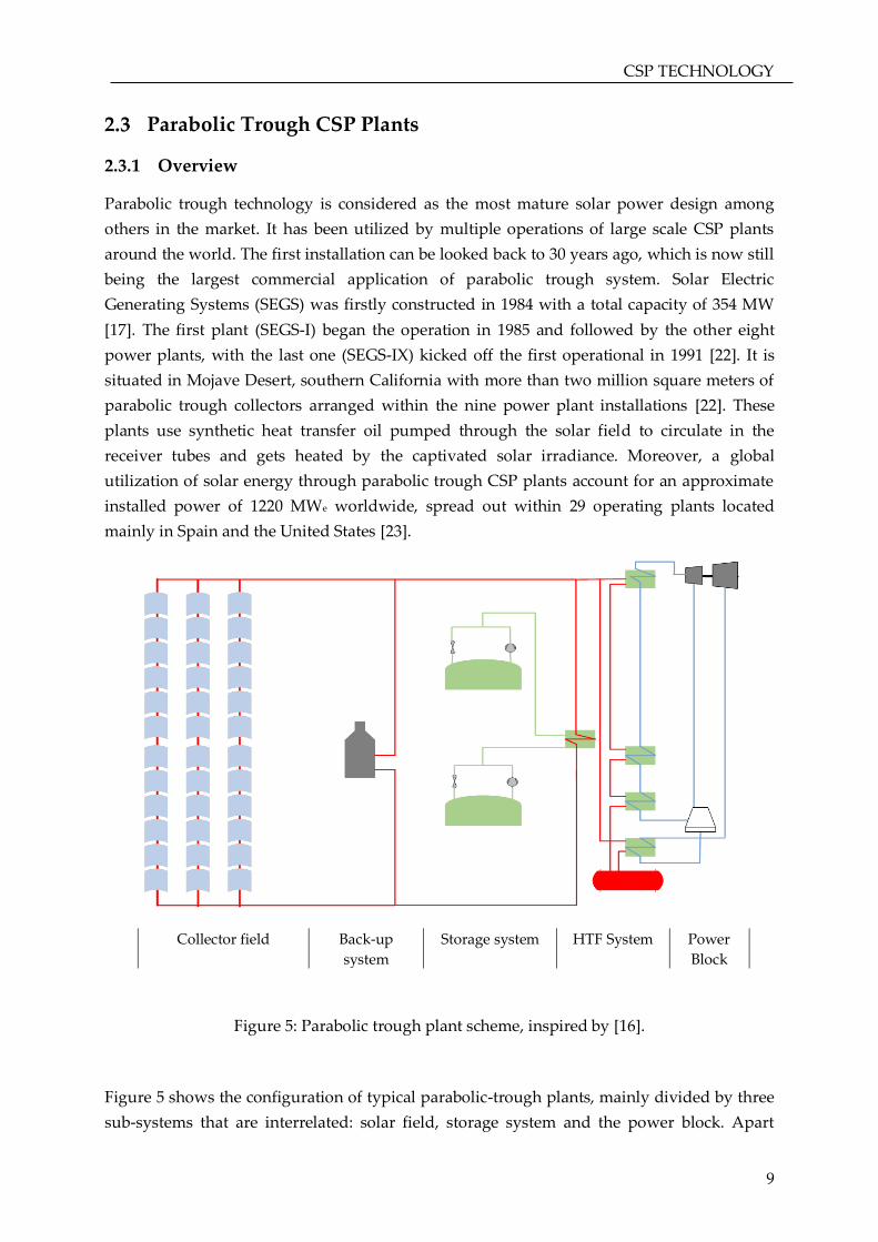
Figure 5: Parabolic trough plant scheme, inspired by [16].

Figure 5 shows the configuration of typical parabolic-trough plants, mainly divided by three

sub-systems that are interrelated: solar field, storage system and the power block. Apart

CSP TECHNOLOGY

10

from these components, some CSP plants may also have a back-up system consisting of an

auxiliary heater, the unit located in between the solar field and storage system, used to allow

the plant operation when solar radiation and thermal energy in the storage are not available.

Some plants may also locate the auxiliary heater in the power block, enabling the production

of superheated steam for the steam turbine directly. This configuration is estimated to give

higher overall plant efficiency compared to the solar field auxiliary heater because it reduces

the possibility of producing thermal losses in the oil circuit [20].

• The Solar Field

The cornerstone of parabolic trough plant is the solar field, which consists of all components

constructed to one another, with several Solar Collector Assemblies (SCA’s) are attached to

form a single or multiple loops, with each loop arranged in parallel. Each SCA is composed

of a number of parabolic trough collector modules laid out in series and Heat Collection

Elements (HCE) installed at the focal line of the parabolic surface. This is a block where solar

radiation is captured and converted into thermal energy in the form of sensible heat carried

by the working fluid that flows within the receiver tubes and piping system to the storage or

power block.

The collector loops are connected to the cold and hot header, allowing the flow of heat

transfer fluid into each loop. One header pipe transports the cold HTF to be heated up in the

solar field and another header collects the hot HTF to distribute it to the power block for

power generation and/or to the thermal energy storage for use at later time under special

circumstances.

• Thermal Energy Storage System

As shown in the center of Figure 5, there are dual tanks functioning as hot and cold tank

which are part of the storage system. In between them, heat exchanger is placed to allow an

efficient transfer of heat from the solar field working fluid to the storage medium. Thermal

energy storage system is not an essential unit in the operation of CSP plants. However, it

provides clear benefits to the plant operation, such as increases the operating hours per year,

enhances the operation under cloudy periods as well as improves the dispatchability under

different strategies that can be developed by the operator to allow higher financial income.

• Power Block

This sub-system converts thermal energy delivered from the solar field or the storage system

into electricity. It is by means of a typical Rankine cycle that comprises of several

components: pumps, cooling systems, steam turbine, electricity generator and water/steam

heat exchangers. Typically on a clear day, the solar field receives DNI in the range of 100 –

300 W/m2 [20] and the working fluid recirculates through the solar field until it reaches the

nominal outlet temperature. The fluid transfers the thermal energy to another sub-system,

either thermal energy storage or steam generator to rotate the turbine and start the power

block. In summer months, the solar field receives high amount of solar radiation, sufficient to

CSP TECHNOLOGY

11

keep the power block running at full load during the daylight hours as well as to charge

thermal energy storage. However, the thermal output of solar field during daylight times on

clear winter days is much less than in summer, for which only suffices to feed the power

block.

2.3.2 Solar Field Components

The setting of parabolic trough CSP plants comprises of several elements constructed as the

following:

2.3.2.1 Piping layout

Large commercial parabolic trough systems comprise of collectors aligned in parallel rows

which are connected to one another and forming a layout of solar field. There are three basic

layouts used in parabolic trough solar fields, named as direct-return, reverse-return and the

center-feed. The direct-return configuration is the simplest layout and the most extensively

used in small-sized solar fields. The main advantage of this layout is the relatively low

occurrence of thermal losses in the piping system. The working fluid flows into the receiver

tube from one direction and will flow out into from the opposite direction. In the

arrangement, the length of the inlet and outlet pipes is equal in order to prevent an

installation of long pipe in the system, which can benefit to reduce the piping costs. On the

other hand, the disadvantage of this layout is the high pressure difference between the row

inlets that are installed in parallel, which implies in the necessity to install additional valves

to keep a constant flow of heat transfer fluid. These valves, in fact bring the second drawback

which is the increase of pressure drop in the solar field that directly contributes in the

enhancement of pressure loss in the CSP plant system [20].

Direct-return Reverse-return

Figure 6: Direct and reverse-return piping layout, inspired by [20].

In the reverse-return layout as seen in Figure 6, the heat transfer fluid enters the receiver

tube mounted at the focal line of the collector arrays from one direction. The rows with a

longer inlet pipe will have a shorter outlet pipe while the rows with a shorter inlet pipe have

a longer pipe to transfer the output. The arrangement allows creating an approximately

CSP TECHNOLOGY

12

equal flow resistance between different rows of solar collectors and reduces the pressure

drop along the piping system of the solar field. Longer pipes, however, mean an increase in

the piping costs due to the requirements to insulate the pipes. An adequate thermal

insulation is of high importance in the solar field piping system to prevent the reduction of

overall efficiency due to high thermal losses.

Figure 7: Center-feed piping layout, inspired by [20].

The center-feed configuration (presented in Figure 7) is the most widely used layout for large

solar fields. It reduces the piping length as there is no pipe installed along the length of

collector and also gives an access to each collector row. As the collectors need a frequent

maintenance and washing, the center-feed layout is more beneficial for these occasions.

2.3.2.2 Heat Collection Element

In the solar field, multiple sets of Solar Collection Assembly (SCA) and Heat Collection

Element (HCE) are composed of parabolic reflector modules and receiver tubes. The tubes

are fixed to the reflector support structure and drive pylons with joints are assembled to

allow a single-axis solar tracking. Moreover, the HTF pipe is attached to allow the flow of

fluid to and from the receivers. SCA’s are laid out in parallel rows with spacing in between

the rows in order to reduce the shading of reflectors by one another. Moreover, this also

benefits in ensuring sufficient access for maintenance, allowing cleaning work for the

reflectors surface from particles that can reduce the efficiency, and minimize the parasitic

pumping energy for the heat carrier when the solar field is not under operational mode [24].

The distance between the rows is an important concern in outlining the power plant, which

should not be too small or too big. The shading will potentially increment if the distance

between rows is too small, while inversely it will require a long pipe network which directly

imply to an increasing thermal losses [19].

The heat collection element of parabolic trough plant consists of the receiver tubes, having

the task to convert solar radiation that is reflected to them into heat and to transport this heat

along the piping systems to the destination, either the power block or thermal energy

storage. In order to have a high production of thermal energy, it is important to ensure that

CSP TECHNOLOGY

13

the receiver tubes absorb a maximum radiant solar flux and have minimum thermal losses.

The thermal losses refer to three different mechanisms; radiation, convection and

conduction. To achieve the aforementioned goal, there are two important constraints:

geometry and physical condition must be taken into account.

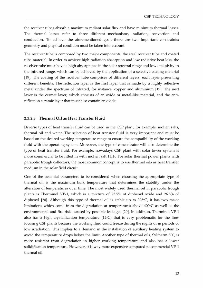
The receiver tube is composed by two major components: the steel receiver tube and coated

tube material. In order to achieve high radiation absorption and low radiative heat loss, the

receiver tube must have a high absorptance in the solar spectral range and low emissivity in

the infrared range, which can be achieved by the application of a selective coating material

[19]. The coating of the receiver tube comprises of different layers, each layer presenting

different benefits. The reflection layer is the first layer that is made by a highly reflective

metal under the spectrum of infrared, for instance, copper and aluminium [19]. The next

layer is the cermet layer, which consists of an oxide or metal-like material, and the anti-

reflection ceramic layer that must also contain an oxide.

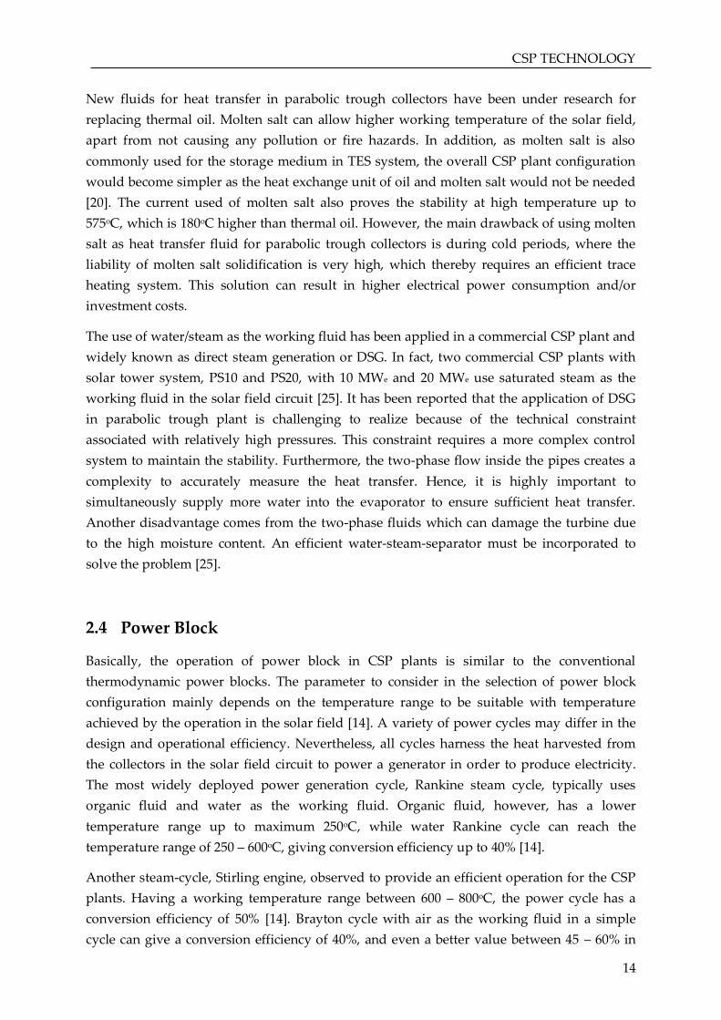
2.3.2.3 Thermal Oil as Heat Transfer Fluid

Diverse types of heat transfer fluid can be used in the CSP plant, for example: molten salts,

thermal oil and water. The selection of heat transfer fluid is very important and must be

based on the desired working temperature range to ensure the compatibility of the working

fluid with the operating system. Moreover, the type of concentrator will also determine the

type of heat transfer fluid. For example, nowadays CSP plant with solar tower system is

more commercial to be fitted in with molten salt HTF. For solar thermal power plants with

parabolic trough collectors, the most common concept is to use thermal oils as heat transfer

medium in the solar field circuit.

One of the essential parameters to be considered when choosing the appropriate type of

thermal oil is the maximum bulk temperature that determines the stability under the

alteration of temperatures over time. The most widely used thermal oil in parabolic trough

plants is Therminol VP-1, which is a mixture of 73.5% of diphenyl oxide and 26.5% of

diphenyl [20]. Although this type of thermal oil is stable up to 395oC, it has two major

limitations which come from the degradation at temperatures above 400oC as well as the

environmental and fire risks caused by possible leakages [20]. In addition, Therminol VP-1

also has a high crystallization temperature (12oC) that is very problematic for the line-

focusing CSP plants because the working fluid could freeze during the nights or in periods of

low irradiation. This implies to a demand in the installation of auxiliary heating system to

avoid the temperature drops below the limit. Another type of thermal oils, Syltherm 800, is

more resistant from degradation in higher working temperature and also has a lower

solidification temperature. However, it is way more expensive compared to commercial VP-1

thermal oil.

CSP TECHNOLOGY

14

New fluids for heat transfer in parabolic trough collectors have been under research for

replacing thermal oil. Molten salt can allow higher working temperature of the solar field,

apart from not causing any pollution or fire hazards. In addition, as molten salt is also

commonly used for the storage medium in TES system, the overall CSP plant configuration

would become simpler as the heat exchange unit of oil and molten salt would not be needed

[20]. The current used of molten salt also proves the stability at high temperature up to

575oC, which is 180oC higher than thermal oil. However, the main drawback of using molten

salt as heat transfer fluid for parabolic trough collectors is during cold periods, where the

liability of molten salt solidification is very high, which thereby requires an efficient trace

heating system. This solution can result in higher electrical power consumption and/or

investment costs.

The use of water/steam as the working fluid has been applied in a commercial CSP plant and

widely known as direct steam generation or DSG. In fact, two commercial CSP plants with

solar tower system, PS10 and PS20, with 10 MWe and 20 MWe use saturated steam as the

working fluid in the solar field circuit [25]. It has been reported that the application of DSG

in parabolic trough plant is challenging to realize because of the technical constraint

associated with relatively high pressures. This constraint requires a more complex control

system to maintain the stability. Furthermore, the two-phase flow inside the pipes creates a

complexity to accurately measure the heat transfer. Hence, it is highly important to

simultaneously supply more water into the evaporator to ensure sufficient heat transfer.

Another disadvantage comes from the two-phase fluids which can damage the turbine due

to the high moisture content. An efficient water-steam-separator must be incorporated to

solve the problem [25].

Power Block

Basically, the operation of power block in CSP plants is similar to the conventional

thermodynamic power blocks. The parameter to consider in the selection of power block

configuration mainly depends on the temperature range to be suitable with temperature

achieved by the operation in the solar field [14]. A variety of power cycles may differ in the

design and operational efficiency. Nevertheless, all cycles harness the heat harvested from

the collectors in the solar field circuit to power a generator in order to produce electricity.

The most widely deployed power generation cycle, Rankine steam cycle, typically uses

organic fluid and water as the working fluid. Organic fluid, however, has a lower

temperature range up to maximum 250oC, while water Rankine cycle can reach the

temperature range of 250 – 600oC, giving conversion efficiency up to 40% [14].

Another steam-cycle, Stirling engine, observed to provide an efficient operation for the CSP

plants. Having a working temperature range between 600 – 800oC, the power cycle has a

conversion efficiency of 50% [14]. Brayton cycle with air as the working fluid in a simple

cycle can give a conversion efficiency of 40%, and even a better value between 45 – 60% in

CSP TECHNOLOGY

15

the combined cycle. However, this type of power cycle must be operated under a very high

temperature above 850oC in order to reach these efficiency values. This is a big challenge for

the CSP plants because the existing and mostly deployed thermal energy storages integrated

in the power plants are not capable to operate under extreme temperatures from the material

side. In addition, the receivers in the solar field also have the same limitation to handle the

operating temperatures of the cycle [14]. Commercially, all large-scale CSP plants use the

Rankine cycle for electricity generation. The technology is considered the most mature and

has low risks. With the operating temperature range offered, it is compatible with the CSP

plant technologies, such as parabolic trough, solar tower and linear Fresnel system.

Thermal Energy Storage

2.5.1 Overview

A prominent complication in the solar energy utilization is the intermittent availability of the

source, which imply to the imbalance production throughout the day, or even throughout

the year. In the CSP plants, thermal energy storage (TES) serves multiple functions. It

balances out the plant under variable weather conditions. For instance, when the clouds

cover the sky over the solar power plant location, it can cause a transient change in the

variable supply of solar flux. It may severely affect the function of turbine because of the

operational change to a significant decrease of load. The integration of thermal storage here

can enable stability in the turbine by offering a base load operation. Moreover, TES can store

solar energy collected during daytime to be converted into electricity in the power block. It

allows a supply of electricity to be fed into the grid during subsequent peak demand periods.

The major requirements on the thermal energy storage systems for CSP plant rely on several

parameters; charge and discharge heat rates, energy capacity, sensible or latent heat storage,

maximum and minimum temperatures, thermal and chemical stability for the number of

cycles and the heat losses [26]. The most widely applied thermal energy storage in CSP

plants typically includes a dual-tank thermal storage that uses molten salt as the thermal

storage medium. It is considered as the most mature technology for both parabolic trough

and solar tower power plants. The salt used in the thermal storage system is commonly a

mixture of 60% sodium nitrate (NaNO3) and 40% potassium nitrate (KNO3) [20]. Unlike solar

tower system that has a dual-tank direct system, for which the molten salt is used as heat

transfer fluid as well as storage medium, in parabolic trough CSP plant, thermal energy

storage is applied as an indirect system because it mainly uses thermal oil as the thermal-

absorbing fluid.

The classification of thermal storage based on the methods of storing energy and heat

transfer mechanism is explained as the following:

CSP TECHNOLOGY

16

2.5.2 Classification of TES according to the methods

Commonly, there are three common types of energy storage based on its methodology in

storing energy: sensible, latent and thermochemical.

• Sensible heat storage

The principle of sensible thermal energy storage system is that either solid or liquid, will

undergo temperature changes when it stores and releases thermal energy. This temperature

change does not cause another variation and therefore, sensible heat storage is considered as

a low-cost storage system. Moreover, sensible heat storage is capable to employ a wide range

of solid and liquid materials. With a solid material, heat exchange fluid will flow through it

inside the TES. The system is advantageous in term of the process and the use of inexpensive

solids as storage materials, such as silica bricks and concretes [17]. But solids are considered

to have low heat density, making the storage process in-efficient [27].

Liquid media, on the contrary, has been widely used in sensible TES system in the form of

molten salts and oils because of their high conductivity and heat capacity [28]. Molten salts,

especially, have come to lead in the application of thermal storage systems in CSP plants. It is

due to the capability of the fluid being used not only as the storage medium but also the heat

transfer fluid. Moreover, the operating temperature of molten salt is very ideal for high

temperature steam turbines in the electricity generation cycle [14].

• Latent heat storage

The second category, latent thermal storage, heats up the storage medium until it melts

down and forms another phase. The process takes place under certain temperature and

involves solid-liquid phase or liquid-vapor phase transitions. The storage medium features

the phase-change phenomena is usually Phase Change Materials (PCM), with organic PCMs

has been proven to have a high energy density and great thermo-physical properties

compared to sensible heat storage materials [14]. It benefits the system as the temperature

during the phase transition can be used as an approximate constant level to control the

system temperature. A disadvantage of PCMs is in their low thermal conductivity, which

results in low charge and discharge rates.

• Thermochemical heat storage

In the thermochemical heat storage, thermal energy forces the endothermic chemical reaction

to form the chemical bonds. This occurs in the storage charge scheme at high temperatures.

Meanwhile, during the storage discharge, the chemical bonds break down under an

exothermic reaction and release thermal energy for electricity generation [17].

Thermochemical heat storage is seen to be compatible for higher temperatures compared to

sensible and latent heat storages.

CSP TECHNOLOGY

17

2.5.3 Classification of TES according to the storage concept

The type of thermal storage system in CSP plants can be either active or passive according to

the heat transfer mechanism between the heat transfer fluid and storage medium.

• Active storage systems

Active storage systems are categorized as direct and indirect-type, which depends on the use

of heat transfer fluid and TES medium. In the active direct thermal storage system, the same

fluid is used as the thermal storage medium as well as heat transfer fluid of the CSP plants.

The active direct storage system employs single or dual-tanks, where the latter is more

commonly used in commercial applications, which is molten-salt two-tank system. A single

tank active direct TES system also uses molten salt, having both hot and cold fluids stored in

the same container and separated by a mechanical barrier. Although the use of single tank

reduces the investment as well as operation and maintenance cost, the tank and the barrier

would disclose to thermal stresses [14]. Therefore, this concept has not been used

commercially in the CSP plants.

In the active indirect storage, thermal energy in heat transfer fluid is sent to the storage

medium through heat exchanger. The storage system comprises of dual tanks. The working

principle of the active indirect thermal storage system in parabolic trough system is that the

heat transfer fluid, commonly thermal oil from collectors’ field enters the heat exchanger,

while molten salt in the cold storage tank enters the heat exchanger form the opposite

direction. In this process, thermal oil will have temperature reduction as it is cooled down,

while on the other hand, molten salt is heated up to a higher temperature. This process is

called charging of the storage system. Differently, in the discharging process, thermal oil and

molten salt enter the heat exchanger from the opposite of the charging process and thermal

energy is released from molten salt to be sent to the power block [2]. The dual-tank indirect

storage system offers an advantage that the thermal storage medium does not have to go

through the solar field as it only flows only in between the cold and hot tank. Having two

tanks, however, require higher investment cost as well as operational and maintenance

expenses.

CSP TECHNOLOGY

18

Figure 8: Active direct (left) and indirect (right) TES system, inspired by [25]

• Passive thermal energy storage

In the passive-type thermal storage system, the storage medium does not circulate and is

mainly a solid type medium, such as concrete or solid PCM. Thermal charging and

discharging process fully rely on the circulation of heat transfer fluid that distributes thermal

energy to the solid material through a heat exchanger integrated in the system [14]. This

storage system offers advantages in the low-cost storage materials compared to the other

systems and a high heat exchange rate. However, the disadvantages come from the

additional cost of heat exchanger and the instability that might occur during long operational

periods.

2.5.4 Selection of thermal storage medium

A variety of thermal storage mediums are used in CSP plants, mainly include synthetic oil,

molten salt, steam, PCM and inorganic non-metallic and chemical materials. It is important

to understand the property of these fluids in order to serve as the thermal storage medium.

Among the properties, the fluids must be non-toxic, non-flammable and non-explosive.

Moreover, it is also essential for the fluids to have a high boiling point and low freezing

point to avoid the use of auxiliary heater in the system operation. Temperature of the

ambience may drop significantly at particular period of time due to weather transient and

the exchange heat convection/conduction to surroundings can significantly drop the

temperature of storage medium as well.

DESCRIPTION OF MODELING APPROACH

19

3 DESCRIPTION OF MODELING APPROACH

This chapter explains the modeling approach in detail to cover methodologies and equations

used in the calculation of each power plant sub-system and dispatching strategies. The

whole power plant is divided into smaller sub-systems, such as solar field, power block and

thermal energy storage. The division into several functional units reduces the complexity of

modeling and sets the arrangement of inputs and outputs in a more specific way. Figure 9

shows the three sub-systems and the outflow of the solar field thermal energy output to

either TES or the power block.

Figure 9: Schematic thermal flow in the modeling of parabolic trough CSP plant.

The model of the whole system is developed in MATLAB®. The modeling approach is broken

down into three major parts (as seen in Figure 10): development of solar field model, model

validation and calculation of electrical output from the power block. In order to perform the

simulation, several data are required as input. In the following sections, the aforementioned

parts are described in further detail.


20

Figure 10: Block diagram of detailed modeling approach.

Solar Field Model Description

The solar field comprises of solar collection assembly and heat collection element

components. The working principle of parabolic trough collectors is to utilize solar energy to

the largest extent by tracking the sun and concentrate direct solar irradiation. Thermal

energy obtained is carried by heat transfer fluid to the power cycle. The important

parameters of the solar field model are composed by geographical and weather forecast data,

components geometry, and relevant information for thermal simulation. The simulation code

was designed to function according to the temporal resolution of the input meteorological

data given for every hour.

There are three major stages in the solar field design: definition of the collectors’

characteristics, calculation of absorbed thermal power and thermal process for calculation of

the corrected thermal power. Each of these stages comprises of a detailed calculation as

described on the following.

3.1.1 Definition of Collector Characteristics

The definition of the collector characteristics is performed according to the parameters of

solar time, incidence angle and Incidence Angle Modifier (IAM), collector efficiency, row

shading and end loss factors. The parameters are a function of other fixed parameters and

described in the following:

• Solar Time

The initial process is to calculate the solar time from the local time of the operating CSP

plant. The solar time (𝑡solar ) defines the exact position of the sun passing the meridian at

noon, which is dependent on the specific location. For example, at 12:00 the sun is in the

north, in the southern hemisphere, or in the south, in the northern hemisphere. It is more


21

common to use the solar time compared to the standard time of the location in the simulation

of solar technologies due to the divergence between the longitudes of the observer under the

same standard time [2]. Daylight savings in the code formulation (represented as

𝑡zone correction) can be set up to 1 if the simulated region considers it for particular months of

the year. The equation of time (EoT) is used for the time correction due to the earth

movement. This depends on the angle for time correction (B) and the number of day (𝑁day) in

the year. The expressions to calculate the solar time for a given hour, day, month and year

are as follow [29]:

𝐵 = 360 ∗(𝑁day −81)

364 , (1)

𝐸𝑜𝑇 = (9.87 sin(2𝐵) − 7.53 cos(𝐵) − 1.5 sin(𝐵)) / 60 , (2)

𝑡𝑠𝑜𝑙𝑎𝑟 = 𝑙𝑜𝑐𝑎𝑙 𝑡𝑖𝑚𝑒 (hour) + 𝐸𝑜𝑇 + 𝑡zone correction . (3)

• Incidence Angle and Incidence Angle Modifier

The next step of the modeling is to measure the incidence angle (𝜃) and incidence angle

modifier (IAM) on the collector’s aperture area. The solar incidence angle is defined as the

angle between the sun’s incident radiation and the normal to collector’s aperture area. At

some points of time, the collector area may not be perpendicular to the sun rays by some

certain of angles that reduce the apparent aperture area. These angles are the optical loss that

administers to the reduction of intensity of the sun beam incident on the surface of

concentrator [23]. The variation of the angle of incidence for concentrating solar collectors

depends on the collector alignment and sun position. In the case of a single-axis tracking

system, the variation of angle of incidence is derived from the SolPos model developed by

NREL [30]. The incidence angle factor (𝜃𝑓) depends on parameters such as the angle between

the vertical to the aperture normal or also known as the tilt angle of the tracking axis (𝛼𝑡),

solar altitude angle (𝛼), solar azimuth angle (𝛼𝑠), collector azimuth angle (𝛼𝑐). According to

that, the following calculations are performed:

𝜃𝑓 = cos(𝛼 − 𝛼𝑡) − cos 𝛼𝑡 . cos 𝛼 . (1 − cos 𝛼𝑠 − 𝛼𝑐), (4)

cos 𝜃 = √𝜃𝑓. (5)

The incidence angle modifier (IAM) refers to the changing of optical properties with the

variation of incidence angle [23]. The incidence angle modifier calculation is determined

using an empirical formula expressed in (6), where 𝑎𝑎 , 𝑎𝑏 , 𝑎0,1,2,3,4,5 represent the constants

called incidence angle modifier coefficients [31]. These values are provided by the

manufacturer of collectors.

𝐼𝐴𝑀 = (1 − 𝑎𝑎 + 𝑎𝑎 ∗ cos 𝜃) . (𝑎𝑏 − cos 𝜃) + 𝑎0 + 𝑎1 ∗ 𝜃 + 𝑎2 ∗ 𝜃2 + 𝑎3 ∗ 𝜃3 +

𝑎4 ∗ 𝜃4 + 𝑎5 ∗ 𝜃5.

(6)


22

• Collector Efficiency

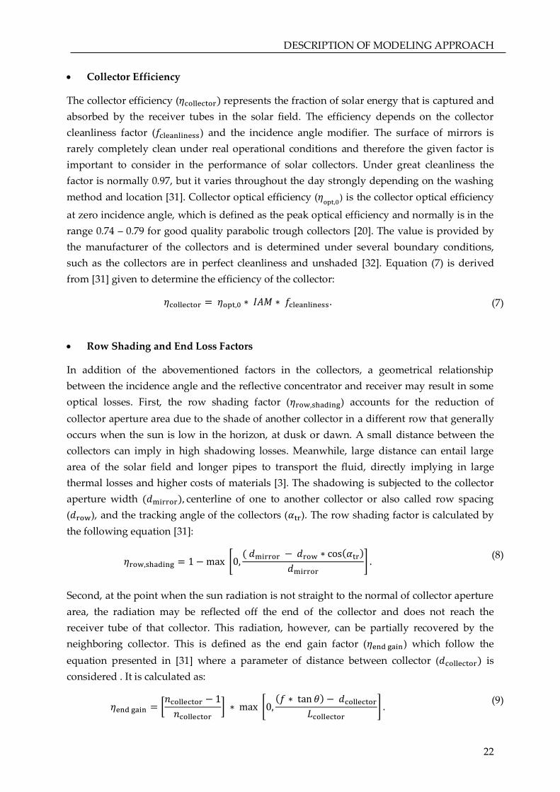
The collector efficiency (𝜂collector) represents the fraction of solar energy that is captured and

absorbed by the receiver tubes in the solar field. The efficiency depends on the collector

cleanliness factor (𝑓cleanliness) and the incidence angle modifier. The surface of mirrors is

rarely completely clean under real operational conditions and therefore the given factor is

important to consider in the performance of solar collectors. Under great cleanliness the

factor is normally 0.97, but it varies throughout the day strongly depending on the washing

method and location [31]. Collector optical efficiency (𝜂opt,0

) is the collector optical efficiency

at zero incidence angle, which is defined as the peak optical efficiency and normally is in the

range 0.74 – 0.79 for good quality parabolic trough collectors [20]. The value is provided by

the manufacturer of the collectors and is determined under several boundary conditions,

such as the collectors are in perfect cleanliness and unshaded [32]. Equation (7) is derived

from [31] given to determine the efficiency of the collector:

𝜂collector = 𝜂opt,0 ∗ 𝐼𝐴𝑀 ∗ 𝑓cleanliness . (7)

• Row Shading and End Loss Factors

In addition of the abovementioned factors in the collectors, a geometrical relationship

between the incidence angle and the reflective concentrator and receiver may result in some

optical losses. First, the row shading factor (𝜂row,shading) accounts for the reduction of

collector aperture area due to the shade of another collector in a different row that generally

occurs when the sun is low in the horizon, at dusk or dawn. A small distance between the

collectors can imply in high shadowing losses. Meanwhile, large distance can entail large

area of the solar field and longer pipes to transport the fluid, directly implying in large

thermal losses and higher costs of materials [3]. The shadowing is subjected to the collector

aperture width (𝑑mirror), centerline of one to another collector or also called row spacing

(𝑑row), and the tracking angle of the collectors (𝛼tr). The row shading factor is calculated by

the following equation [31]:

𝜂row,shading = 1 − max [0,( 𝑑mirror − 𝑑row ∗ cos(𝛼tr)

𝑑mirror] .

(8)

Second, at the point when the sun radiation is not straight to the normal of collector aperture

area, the radiation may be reflected off the end of the collector and does not reach the

receiver tube of that collector. This radiation, however, can be partially recovered by the

neighboring collector. This is defined as the end gain factor (𝜂end gain) which follow the

equation presented in [31] where a parameter of distance between collector (𝑑collector) is

considered . It is calculated as:

𝜂end gain = [𝑛collector − 1

𝑛collector] ∗ max [0,

(𝑓 ∗ tan 𝜃) − 𝑑collector

𝐿collector] .

(9)


23

Whereas only some collectors can incur the end gain energy, all collectors acquire end-loss

effect (𝜂end loss), which is the deviation of reflections from the collectors to the receivers. This

factor accounts for a reduction of effective mirror area induced by the parabolic focal length

(f), incidence angle (𝜃), and the collector length (𝐿collector). This indicates that even two

collectors with the same focal length may undertake diverse influences of the end-loss factor.

The end-loss factor follows the equation in [31] and it is calculated as:

𝜂end loss = 1 − (𝑓 ∗ tan 𝜃)

𝐿collector+ 𝜂end gain.

(10)

3.1.2 Calculation of Absorbed Power

The available solar radiant power (�̇�avail) in a single collector is obtained with equation (11),

as the product of direct normal irradiance and the non-ideal reflective system from various

optical losses. These losses are the products of geometrical imperfection, shading and

aberration of the design shape of collector which are already explained in 3.1.1. The

calculation is formulated as in the following.

�̇�avail = [𝐷𝑁𝐼 ∗ cos 𝜃 ∗ 𝜂end loss ∗ 𝜂row,shading]. (11)

The sun rays are reflected by the collector and fallen into the intercept area of the receiver.

The optical loss in the receiver reduces the available power with a ratio of optical efficiency.

This is called the absorbed power (�̇�abs), measured for a single collector. The calculation is

performed according to (12).

�̇�abs = �̇�avail ∗ 𝐴eff,collector ∗ 𝜂collector . (12)

Furthermore, the absorbed power in the solar field (�̇�absSF ) can be obtained as an accumulative

power in the n-collectors of all n-rows as presented in following equation.

�̇�absSF = �̇�abs ∗ 𝑛row ∗ 𝑛collector . (13)

3.1.3 Calculation of Usable Thermal Power

The heat transfer fluid (HTF) in the solar field circulates through the loops. The absorbed

heat is used to gradually increase the fluid temperature until it reaches the desired field

outlet temperature. Generally, the thermal losses are governed by the mechanisms of

radiation, convection and conduction under temperature conditions and it takes place in

different components, mainly receivers, pipes and vessels.

• Receiver Tube Heat Loss

The thermal loss in receiver tubes (�̇�loss,rec) occurs both in the receiver tube and the glass

tube caused by radiation, convection and conduction. At the receiver tube, the radiative heat

loss is an assertive parameter because the tube warms up to a high temperature and loss its

thermal energy to the surroundings. On the other hand, the convection loss is more


24

dominant at the glass tube due to the flow of surrounding air around the glass receiver [19].

The developed model only considers the heat loss caused by radiation and does not take into

account the convective and conductive heat loss in a specific way, considering that radiation

losses is more significant than the other ones. The radiative heat loss in receiver tubes is

derived from the alteration of the solar flux incident, IAM, effective mirror area, heat loss

coefficients (𝑏0,1,2,3,4) and temperature difference (∆𝑇). The calculation is expressed in (14).

The temperature difference (∆𝑇) is defined as the difference between an arithmetic average

of the heat transfer fluid inlet and outlet temperature with the ambient temperature.

�̇�lossrec = (𝑏0 ∗ 𝐼𝐴𝑀 ∗ �̇�avail + 𝑏1 + ∆𝑇 ∗ (𝑏2 + ∆𝑇 ∗ (𝑏3 + ∆𝑇 ∗ 𝑏4) )) ∗ 𝐴eff,collector ∗ ∆𝑇. (14)

• Pipe and Expansion Vessel Heat Losses

The piping system in the model accounts for the losses associated with a variety of

components. These components in the solar field include hot and cold headers, runners from

the power block to and from the solar field headers, expansion loops, connectors between

loops and headers, and rotating ball joints. The length of the pipes is an important

information to calculate theoretical thermal inertia. Meanwhile, the pipe loss (�̇�loss,pipe) in the

model refers to a simplified assemble respective to the aperture area of the solar field and the

temperature divergence. The pipe loss coefficient (𝑝loss) in W/m2K is used in the calculation

for a specific type of pipe material. A further loss parameter defined in the model is the heat

loss in the expansion vessel (�̇�loss,vessel), for which similar condition is implemented with

vessel loss coefficient (𝑣loss) that is also determined according to the type of material. The

equations [31] are presented as the following:

�̇�losspipe

= 𝐴eff,collector ∗ 𝑛row ∗ 𝑛collector ∗ 𝑝loss ∗ ∆𝑇, (15)

�̇�lossves = 𝐴eff,collector ∗ 𝑛row ∗ 𝑛collector ∗ 𝑣loss ∗ ∆𝑇. (16)

The equations above omit the radiation heat loss in the pipeline and vessel. The decision is

taken because the temperature difference between the outer surface of pipe and vessel with

the ambient temperature is relatively small [32]. The loss mechanisms in the abovementioned

main components yield in the reduction of the absorbed power in the solar field. Hence, the

calculation is performed as in the following equation.

�̇�usableSF = �̇�abs

SF − (�̇�lossrec + �̇�loss

pipe+ �̇�loss

ves ). (17)

3.1.4 Calculation of Corrected Thermal Power

The calculation of corrected thermal power (�̇�corrSF ) in the solar field is an iterative process

that can be solved employing the HTF temperature dependent data using the temperature of

the preceding time step. In the first time step, the model assumes the HTF mean

temperature (𝑇meanfluid) is equal to the freeze protection temperature (𝑇freeze,protection)


25

because it is the minimum temperature the fluid can reach. Freeze protection temperature is

designed to hold the fluid from freezing due to a significant reduction of ambient

temperature and non-existent of solar irradiation.

The solar field is modeled to have four possible main operating modes, mainly to simulate

the impact of transient processes: significant cool-down, heat-up, cool-down and steady-state

(normal operation). Each of these modes is unique and specific in the way inputs and

outputs are handled in the calculation. The main variables that determine each operating

mode are the operating mean HTF temperature to the nominal HTF temperature (𝑇normfluid)

and the usable thermal power (�̇�usableSF ) produced in each time step. The time step follows

the real time sequence which represents the time progression. The time (𝑡) is defined as 𝑡𝑖 =

𝑖 ∗ ∆𝑡, and 𝑖 = 1,2,3,4 … , 𝑛 [7]. The conditions for the determination of the operating modes

can be seen in Figure 11.

Figure 11: Schematic overview of solar field operation modes.

The significant cool down operation mode encompasses the situation where the collectors do

not receive DNI. This is represented by the non-positive �̇�usableSF and HTF mean temperature

below the nominal one. To prevent freezing of the HTF, the fluid temperature is hold above


26

the given freeze protection temperature that is also above the ambient temperature. This

implemented condition also avoids an extremely high power to start-up the solar field in the

next hours for the normal operation. The correction term is the product of significant cool-

down is calculated as in the following:

�̇�corrSF = �̇�usableti

SF (18)

The next operating mode is heat up or start-up of the solar field, defined when �̇�usableSF at

current time step is greater than the previous time step. When the collectors receive sufficient

solar energy on the aperture, it also produces a corresponding thermal energy in the solar

field. The produced thermal energy may be used for self-consumption to heat up the solar

field and the excess heat can be sent to another sub-system. The given equations are used

under the start-up operation and resulting in start-up thermal energy (𝑄startup 𝑆F ) with an

inclusive function of thermal inertia (𝑐SF) to represent the physical property of the material.

The minimum value is taken from the usable thermal power and theoretical solar field

startup thermal energy and it is defined as the actual thermal energy (𝑑𝑄startupSF ) consumed

for the start-up of solar field. The minimum value is taken to ensure required thermal energy

for the operation mode meets the usable thermal power in the solar field. The corrected

thermal power is obtained as the maximum between zero to the subtraction of usable

thermal power with the actual startup thermal energy at the time step (𝑡). The maximum is

taken to prevent negative manner of the corrected thermal power.

𝑄startupSF = 𝑐SF ∗ (𝑇normfluid − 𝑇meanfluid (𝑡i−1)), (19)

𝑑𝑄startupSF = min[�̇�usable

SF ∗ 𝑡, 𝑄startupSF ], (20)

�̇�corrSF = max[0, �̇�usable

SF − 𝑑𝑄startupSF / 𝑡] (21)

Unlikely to the start-up operation mode, the cool down mode is defined when the usable

thermal power (�̇�usableSF ) in the current time step is lower compared to the previous time step.

This phenomenon is due to decreasing direct solar radiation. This operation mode is

expressed in the following equations:

𝑑𝑄cooldownSF = min[�̇�usable

SF ∗ 𝑡, 𝑄avail,downSF ], (22)

�̇�corrSF = 𝑑𝑄cooldown

SF /𝑡, (23)

𝑑𝑄cooldownSF is the actual thermal energy lost due to the cooling down of solar field. It is a

function of the minimum between the usable thermal power and the theoretical cool-down

thermal energy ( 𝑄avail,downSF ). The correction term is obtained as the actual thermal energy

lost from cooling down at the time step.

The last operation mode is steady-state, defined where the HTF temperature reaches the

nominal temperature (𝑇normfluid). Under the specified condition, 𝑇meanfluid shall not exceed


27

the optimum set point and thus it is maintained at the desired temperature. The corrected

thermal power is expressed in the following:

�̇�corrSF = �̇�usableti

SF (24)

Solar Field Model Validation

The validation of the solar field is performed after a complete model of the solar field is

obtained. The validation is important as the basis to analyze if the model developed in

MATLAB works properly. The Greenius software is the validation tool used for a

comparison of the outcomes from the model. The software comes with some example

projects which users may use. The collective meteorological data files with temporal

resolution for the site are entered in a specific format of one-hour time step. The Greenius

software does not support daylight saving time, deriving the calculation of solar time has the

same pattern throughout the year.

As in the next step, users may also define all input data for an economical calculation of the

CSP project, taking into consideration investment costs, operation and maintenance costs

and financing sources, which allow the determination of economic output variables [4].

However, this feature is disabled due to the irrelevant scope with the technical validation of

the solar field. Furthermore, the input component datasets must be designed, which

comprises of different sub-units from the collector assembly and the collector field. Similarly

to the model developed in MATLAB, the same data information of the equipment units is

also used in Greenius software. Thermal energy storage and boiler data arrays are left blank

as they are not featured in the validation. It is important to design the size of an individual

collector in a way it meets the actual accumulative aperture area of the solar field. The

interface of the software can be seen in Figure 12.


28

Figure 12: Interface of the Greenius validation tool in the Collector Assembly.

Once all required input data is defined, the software simulates the calculation very fast and

shows the results in the format table and graphs. These outcomes are used to perform

validation of the solar field through comparison of the outcomes from the model developed

in MATLAB. Apart from result analysis, data plots are also generated in MATLAB to give

greater visualization of model validation by importing the files obtained in Greenius into an

acceptable format.

Calculation of Electrical Output from The Power Block

A certain amount of thermal energy at each point of time is delivered from the solar field to

the power block, for the production of electricity, or TES, to be stored. The calculation of the

power block output is based on the Greenius lookup table, which comprises of three major

selected parameters: thermal input power, ambient temperature and relative ambient

humidity, to obtain a range of power outputs. These attributes are used as references in the

interpolation of a given data of thermal power at every time step, in order to obtain an

electricity output value. In the process, the lookup table is imported to MATLAB and

simulated with the solar field thermal power output data. Detailed information in lookup

table can be found in Appendix B.

The model calculates the amount of electrical power feed-in to the grid at each time step

(𝑃outPB ). The expected financial income (I) from the electricity delivery is obtained according to

the electricity generation (𝑃outPB ) and the electricity price (𝑝el):

𝐼 = 𝑃out PB ∗ 𝑝el. (25)

DISPATCH STRATEGIES

29

4 DISPATCH STRATEGIES

General Concept

Just as other renewable systems, a problem CSP plants faces is the high dependency on the

intermittent solar resource. Throughout the day course, the clouds cover on the sky above

the power plants causes a transient in the sun’s incident rays on the collectors, which is

difficult to forecast. Anyway, forecasting methods are able to provide a reasonable

expectation of future weather, which can then be used to plan the dispatch of CSP plants.

Moreover, CSP plants with integrated thermal energy storage have bigger chance to increase

the economic benefit by shifting the electricity production from periods of low demand to

high demand [33].

In wholesale electricity markets, the power plants should place their bid of electricity

generation for day-ahead. Therefore, accurate weather forecasts are extreme important in

order to obtain a reliable dispatching plan. If in reality there is interference in the absorbed

DNI different to what has been expected, the real electricity generation differs from the

planned scheduled generation. As a result, the CSP plants must bear the risk of paying

penalties for the deviation from the scheduled electrical output fed-in to the grid [34].

The dispatch planning strategies proposed here consist of an innovative algorithms that use

a rule-based approach to plan the electricity generation of CSP plants. The tool tries to

generate an optimal electricity delivery schedule based on weather forecast and electricity

price profile as input (illustrated in Figure 13). For that, the solar field and power block

models, previously described in Chapter 3, are used in order to simulate the plant operation.

The objective of the proposed dispatch planning strategies is to develop an accurate

electricity delivery schedule prioritizing hours with high electricity price in order to obtain

improved financial revenue from the electricity sale.

Figure 13: Modeling scheme of the proposed dispatch planning strategies.

The dispatch strategies plan the thermal input schedule of the power block with the resource

input derived from the solar field performance model presented in 3.1. Deterministic

weather forecast data is designed to simulate the performance of solar field model which

DISPATCH STRATEGIES

30

generates the corrected thermal power. In the CSP plants with parabolic trough collectors,

the working fluids in the solar field and thermal storage are usually different. The thermal

outflow from the solar field leads to two possible schemes, as the flow can be directed either

to the power block or to the storage. Therefore, the dispatch strategies are designed

considering the configuration of CSP plants under two basic operational strategies: solar

driven and storage driven strategy. Under these basic conditions, the schedule still does not

consider optimization aspects. The same optimization criterion is then applied after each of

the basic operational strategies, in order to reach a schedule with delivery during high price

moments.

The proposed dispatch planning strategies are designed to provide several rules which

consist of distinct calculations under different conditions. The rules are set systematically to

execute different choices in order to obtain specific objectives. Each of the basic operational

strategies, either the solar driven or storage driven, is based on specific rules which are

named as basic rules. Based on the solar field thermal output, the algorithms yield in thermal

power input of the power block and the storage, respecting the design values of equipment

in the CSP plant. The solar driven strategy is a standard and most used operation of CSP

plants. The schematic flow is shown in Figure 14, in which the solar field produces thermal

power (�̇�outSF ) to be used as direct and immediate input of the power block (�̇�in

PB). The

objective of this dispatch strategy is to maximize power generation by operating the power

block at full-load as soon as possible.

Figure 14: Scheme of solar driven basic operational strategy.

On the other hand, the storage driven strategy puts an emphasis in the function of thermal

energy storage as a buffer in the operation of CSP plants, as shown in Figure 15. Thermal

energy produced in the solar field (�̇�outSF ) is carried by heat transfer fluid into heat exchanger.

From another direction, the storage working fluid, molten salt, also circulates into heat

exchanger and induces the transfer of thermal energy between the two fluids. Molten salt

flows into the hot storage tank carrying the heat (�̇�inTES) and stores the energy until the CSP

plants need to produce electricity.

DISPATCH STRATEGIES

31

Figure 15: Scheme of storage driven basic operational strategy

As a second step of the proposed dispatch planning strategies, an optimization is performed

in addition to the two dispatch approaches as the basis. Other rules are introduced and they

are named as optimization rules. The general objective of the optimization rules is to

produce a schedule of electricity delivery during hours with high electricity price. It aims for

improved values of financial benefit from the electricity sale in the wholesale market. In

addition, at some points in the day course, an excessive thermal energy might be available

for the system. Due to the limitation of storage to accommodate the heat, during such

moments, the collectors must be defocused. It implies in certain amount of thermal energy

wasted from the solar field which accounts to financial losses. Optimization rules are

formulated to avoid such occurrences, reducing the intentional deflected of potential thermal

energy due to the system boundaries.

Two types of time sequence are used in the dispatch planning rules which are specified

based on the rule’s objective. The basic rules follow the real time sequence, while the

optimization rules follow the time steps sequence that is based on its price value. The time

step sequences are presented as the following:

• Real time sequence:

It follows the real time progression for each time step, where time (𝑡) is defined as

𝑡𝑖 = 𝑖 ∗ ∆𝑡, and 𝑖 = 1,2,3,4 … , 𝑛 [7].

• Decreasing price sequence:

It considers the relation between each time step with the electricity price in a

decreasing manner according to the price. For example, 𝑡1 is the time step with the

highest price value, 𝑡2 is the time step which has the second highest price value, and

so on. This goes until the last time step at 𝑡𝑛 , the one that has the lowest price value.

The illustration of the time sequences can be seen in Figure 16, with 𝑛 = 5 and ∆𝑡 = 1 hour

are set as the time boundary of the simulation process.

DISPATCH STRATEGIES

32

(a) (b)

Figure 16: Example scheme of time sequencing: real-time sequencing (a) and decreasing price

sequencing (b).

Basic Rules

4.2.1 Solar Driven Strategy

The solar driven strategy prioritizes the delivery of thermal energy from the solar field to the

power block at its maximum permissible capacity. The remaining thermal energy from the

solar field is delivered to the storage tank considering the real time sequence, giving an

accumulative storage level with the storage content from the previous time steps. In the end,

it identifies the solar field energy dumped, which is defined as the thermal energy not used

by the system once the power block and TES are in full capacity. The solar driven strategy

ensures the electricity delivery as soon as thermal energy has been produced by the solar

field. However, this strategy is not suitable for an optimal financial objective for the CSP

plants because the electrical output is sent to the grid neglecting the price condition. The

process flow and the basic rules application can be seen in Figure 17 and the rules are

described in the following:

• Basic Rule 1

The basic rule 1 in the solar driven strategy is set for an allocation of solar field thermal

power outflow (�̇�outSF ) as the thermal input power of the power block (�̇�in

PB) in a direct way,

because the core objective is to maximize direct production of electrical power. The

maximum power block input power (�̇�max,inPB ) must be achieved if the thermal output of solar

field is sufficient.

• Basic Rule 2

Excessive solar field thermal power (�̇�excessSF ) is obtained from the subtraction of solar field

thermal power with the power block input power defined by basic rule 1. The excessive solar

field thermal power is defined as thermal energy that cannot be accepted by the power block

due to the PB input limitation. The excess thermal power is transferred to the TES, respecting

DISPATCH STRATEGIES

33

its storage charging limitation (�̇�max,inTES ) and maximum storage capacity (𝑄max,cap

TES ). However,

if all boundary conditions are not fully met, the energy that could be stored in the storage is

the minimum of the three possible values: the excess thermal energy, maximum storage

input and the amount of energy that can be possibly stored in respect to the maximum

capacity of TES and its current level. If charging limitation and capacity reach the maximum,

thermal energy is dumped (�̇�dumpedSF ) and parabolic trough concentrators are defocused.

For the initial time step, the TES is assumed to have certain amount of energy stored in the

system. During the storage charge operation, thermal loss (�̇�lossTES) are considered as a fixed

value for each time step.

DISPATCH STRATEGIES

34

Figure 17: Scheme of basic rules application in solar driven strategy.

DISPATCH STRATEGIES

35

4.2.2 Storage Driven Strategy

The storage driven strategy prioritizes the delivery of thermal energy from the solar field to

the TES system with the objective to, later on once the optimization rules are applied,

schedule electricity production at higher price times. Some boundary conditions are applied,

such as the TES maximum capacity (𝑄max,capTES ) and maximum charging limitation(�̇�max,in

TES ).

The excess SF outflow (�̇�excessSF ) is transferred to the power block to avoid dumping of

thermal energy. The process flow and the basic rules application can be seen in Figure 18.

The process flow is based on the following rules:

• Basic Rule 1:

The thermal energy produced in the solar field is transferred to the storage system. At the

initial time step (𝑡0), TES has an assumed available thermal energy (𝑄chargeTES ) at a certain level.

In the first principle, the transfer of thermal energy to the storage is subjected the storage

charging limitation as well the maximum capacity. Excess SF thermal outflow, defined as

thermal energy that cannot be stored in TES, is transferred to PB, respecting its maximum

capacity.

• Basic Rule 2:

In the second rule, the power that could not be stored is taken as an extra power that can be

sent to the power block. The power block maximum input power is the limiting condition for

this extra solar field thermal power. If PB input thermal flow reaches the maximum limit,

parabolic trough concentrators are defocused and solar field thermal energy dumped

(�̇�dumpedSF ) is obtained.

DISPATCH STRATEGIES

36

Figure 18: Scheme of basic rules application in storage driven strategy.

DISPATCH STRATEGIES

37

Optimization Rules

After the basic rules, an optimization is performed considering the decreasing price

sequence. The system outflow and inflow are re-adapted based on this sequence manner of

the price, prioritizing the electricity production from the power block during higher price

time steps. This means that the schedule previously developed by the basic rules is re-

adapted by the optimization rules. Principally, the optimization of dispatch planning

strategies represents the objectives to generate maximum revenue from the electricity

production and minimize energy dumping. The optimization rules comprise of rule 1 and

rule 2 which are simulated within the same loop based on the decreasing time sequence as

presented by Figure 19. The rules are greatly described in the following sections.

Figure 19: The loop for implementation of optimization rule 1 and 2.

• Optimization Rule 1:

In the first step, the algorithm checks the thermal input power of the power block, that has

been already planned with one of the basic dispatch strategies (solar driven or storage

driven). As the objective is to obtain the maximum financial income from the electricity sale,

it is important to send the maximum power to steam turbine at high price times to produce

the maximum electricity output. Optimization rule 1 distributes the energy in storage from

the higher price time steps to the lower price.

If the power block inflow is not at its maximum input power (�̇�max,inPB ) at 𝑡𝑖 and there is

thermal energy available in the storage, the discharging process will occur, i.e. thermal flow

is sent from TES to PB. This additional thermal power needed to operate the power block in

full load is defined as �̇�1. The possible power in TES to be discharged to the power block for

electricity production is defined as �̇�2, respecting the availability of thermal energy at all

instants from 𝑡𝑖 to 𝑡𝑛 . It is important to take into account thermal energy level until the last

temporal time step of optimization because the TES levels are re-adapted according to the

energy taken at 𝑡𝑖 and it should not lead to an undermine of the storage level.

DISPATCH STRATEGIES

38

Another control parameter, maximum discharge power (�̇�max,outTES ), is set as a boundary

condition, with a lower value compared to the power block maximum input. The decision is

made based on the circumstance of heat transfer mechanism in the heat exchanger which

leads to some energy losses that reduce the final thermal energy output from the storage to

the power block.

In order to respect the boundary conditions and energy balance in the system, the final

energy to be taken from the storage is the minimum of the three possible values: �̇�1, �̇�max,outTES

and �̇�2, also respecting the minimum capacity of TES (𝑄min,capTES ), considered as about 2% of

the maximum capacity. The scheme of optimization rule 1 is presented in Figure 20. The

implementation of the rule’s calculation results in an updated value for the TES level

(𝑄chargeTES ) as well as for the power block input (�̇�in

PB).

DISPATCH STRATEGIES

39

Figure 20: Schematic of optimization rule 1 calculations.

• Optimization Rule 2:

The second rule of optimization in the dispatch planning aims to avoid energy dumping

from the solar field. For that, expected dumped energy resulting from the previously applied

rules is foreseen to be reduced, by being stored when possible. At first, the algorithm

analyzes an available space in the storage at the selected 𝑡𝑖 , as a function of the storage level

and the storage maximum capacity (𝑄max,capTES ) from 𝑡𝑖 to 𝑡𝑛 . Moreover, the dumped thermal

DISPATCH STRATEGIES

40

energy from the same range of time steps is also taken into account. The decision of possible

power to be added to TES input (�̇�in,possTES ) is determined from the minimum of two possible

values: subtraction of TES maximum capacity with the TES level (𝑄chargeTES ) until the last

temporal resolution in decreasing price sequence, and the maximum charging

limitation(�̇�max,inTES ).

A second time sequence is used in this rule application: the real time sequence that identifies

the availability of solar field wasted energy at time step from which thermal energy is taken

out. It is defined as 𝑡𝑗 , where 𝑗 = 1,2, … , 𝑛 and it refers to a condition for which dumped

thermal energy will be stored when it is available in greater time instants compared with 𝑡𝑖.

The storage levels are re-adjusted according to the amount of energy stored and wasted

thermal energy level is also re-calculated. The calculations are performed according to Figure

21.

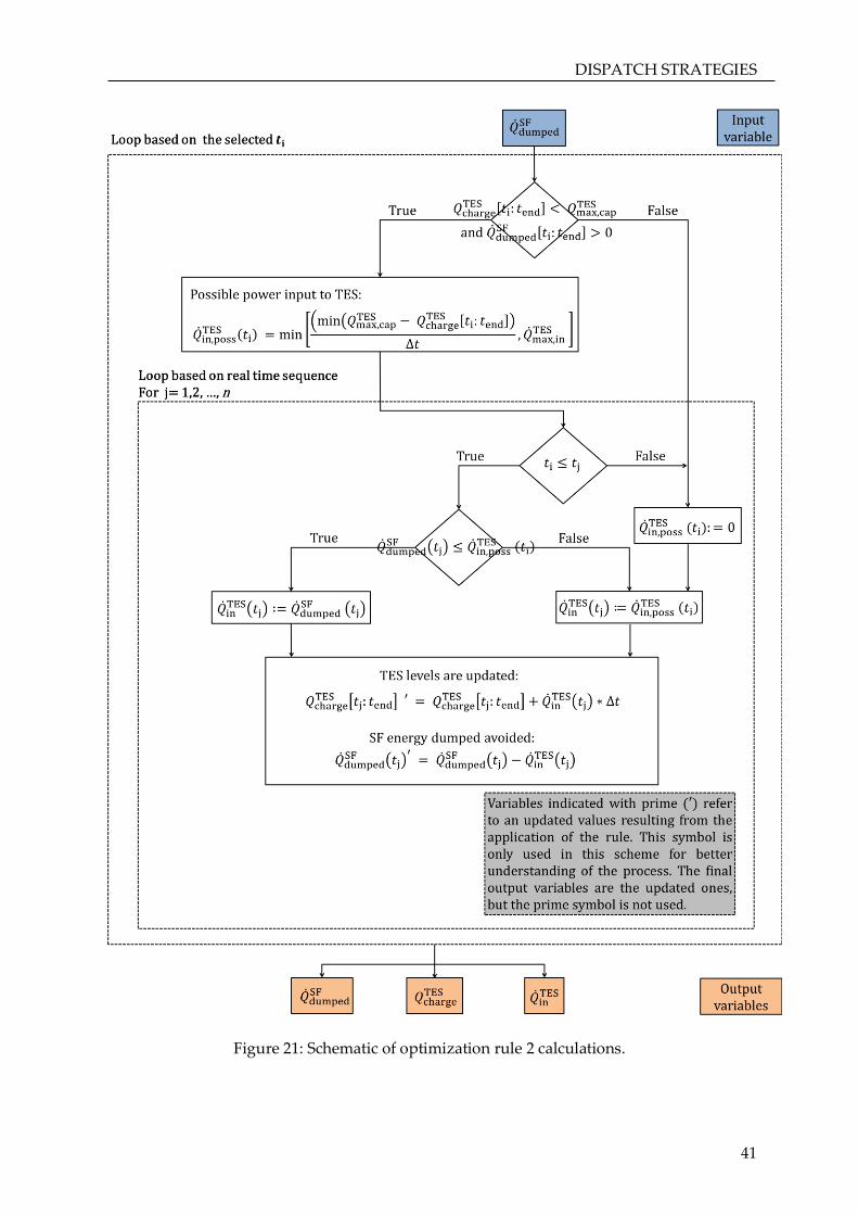
DISPATCH STRATEGIES

41

Figure 21: Schematic of optimization rule 2 calculations.

RESULTS AND REMARKS

42

5 RESULTS AND REMARKS

In this section, the simulation results are presented comprising of five main topics. In the first

part, the reference data is presented to cover the whole parameters taken into account in the

simulation processes. The results are presented according as the result of solar field

simulation, solar field validation, dispatch strategies implementation and the electricity

generation. Further explanations are described in the following sub-chapters.

Reference Data

For the entire simulation processes, several data consisting of weather forecast and technical

properties of the components in the solar field, thermal storage and the power block are

explained in this section. These data are collected based on the parabolic trough La Africana

CSP plant situated in Córdoba, Spain under latitude of 37.7554 °N and longitude -5.0572 °E

with an elevation of 138 m. The reference data is organized according to the function in the

simulation, which is divided into three categories: weather forecast data, solar field data and

properties of TES and PB. Weather forecast data is functional as the input of solar field

simulation and the solar field data represents the technical characteristics of equipment

within the solar field. In addition, the technical properties of TES and power block cover the

technical boundaries of the unit operation. In the following sub-sections, further detail of

each data is presented.

5.1.1 Weather Forecast Data

Weather forecasts are collected from the actual data in the form of direct normal irradiation

(DNI) in W/m2 and ambient temperature in °C for Badajoz area, located near the power

plant. They are an important input to determine the solar field performance from the

production of thermal energy. Spain is located in south Europe and had a daylight savings

scheme that adds one hour to the real time from 29th March to 25th October in 2015.

Moreover, a total of seven days from different months in 2015 are selected for the study with

a temporal resolution of one hour. The selection of the months (January, April, July and

October) are based on consideration to observe the effect of DNI profiles in different seasons:

winter, spring, summer and autumn. The ambient temperature data is used to calculate the

thermal performance of CSP plants. Figure 22 and Figure 23 show the forecasts data of DNI

and ambient temperature, respectively, over the week in the selected months. The selected

days for each of these months are as in the following:

January : Date 15 – 21

April : Date 1 – 7

July : Date 1 – 7

October : Date 1 – 7

RESULTS AND REMARKS

43

From Figure 22, DNI profiles can be observed to have a fluctuate manner throughout the day

course. In winter period in January, DNI forecasts for the selected days are observed to be

the lowest compared to other days in the remaining months, as expected. For this month,

peak irradiance is obtained at 15:00 on the third simulation day (17th January) with a value of

912 W/m2. Because of the angle between the vertical and the Earth’s tilt at 23.5 degrees, the

seasonal variation occurs on Earth [35]. Therefore, direct normal irradiance varies for every

season. In April and October, direct peak irradiances are obtained on the first and seventh

day with values of 952 W/m2 and 914 W/m2, respectively. July receives the highest irradiance

value of only 911 W/m2 on the seventh day at 16:00. This is lower compared to the other

months which have been described previously. Peak irradiance is usually higher in summer

month due to the higher sun angles. The increasing sun angles contribute to reduce the

cosine loss and the optical path length of direct solar irradiance in the atmosphere [36].

Although it cannot be observed in the data of July, it is probably due to the limitation in the

selection of days.

Apart from that, the distribution of DNI over the seven days in January, April and October

are more volatile compared to July. It may be expected as the result of high probability to

have the cloud cover conditions in these three months. In summer time, the sky is usually

clear and it results in a reliable and constant direct normal irradiance throughout the time

period as observed in July.

Figure 22: DNI forecasts data.

Similar trends are shown in the ambient temperature data. The months with low exposure to

the sun are among the cold periods with low ambient temperature. In January, the lowest

temperature reaches 0oC and the highest temperature is measured at 14oC. The temperatures

increase in the following months until July, where they reach the peak points and drop again

in October. In April and July, the highest ambient temperatures are observed at 16:00 in the

noon with a value of 27oC and 37oC respectively. Meanwhile in October, the peak

temperature from the forecast data reaches 29oC.

RESULTS AND REMARKS

44

Figure 23: Ambient temperature forecasts data for the selected days.

5.1.2 Solar Field Characteristics

The technical data of the solar field are listed in Table 1. These data are based on the

configuration of parabolic trough La Africana CSP plant. The solar field consists of 168 loops,

for each one comprises of 4 Solar Collector Assemblies (SCA) and 12 collectors per SCA. The

concentrators are typical Sener Trough model, with a total effective mirror area of 550

thousand m2. The receivers are mounted at the focal line of the parabolic surface, with a

diameter of 70 mm from Schott PR70 model.

Table 1: Input data of solar field geometry.

Solar field geometry

Length of collector 𝐿collector 12 m

Collector diameter 𝑑col 1 m

Collector aperture width 𝑑mirror 5.77 m

Focal length f 1.7 m

Row spacing 𝑑row 17.3 m

Collector optical efficiency 𝜂opt,0

76%

Cleanliness factor 𝑓cleanliness 97%

The orientation of the collectors’ tracking axis is North-South and the solar field heat transfer

fluid used in the reference plant is from the thermal oil class, Therminol-VP1. The mean

temperature of the fluid is an essential parameter in the calculation of corrected thermal

power and its initial value is assumed at 60oC, equal to the freeze protection temperature.

This decision is taken because it is the minimum temperature the fluid can reach. The desired

RESULTS AND REMARKS

45

temperature of the fluid is an average of inlet and outlet temperature for the Therminol VP-1,

with values of 293oC and 393oC, respectively.

5.1.3 Technical Properties of TES and the Power Block

The power block in La Africana CSP plant is typical Rankine cycle with an installed capacity

of 50 MWe. Two-tank indirect storage is installed with one tank behaving as the cold tank

and another one as the hot tank. Thermal storage uses molten salt as the working fluid to

receive the heat from thermal oil and to transfer heat to the power block. The heat transfer

mechanism is possible through the heat exchanger installation. Detailed design and control

parameters of the thermal storage and the power block are shown in Table 2. The storage has

a minimum desired capacity of 2% from its maximum capacity and it is calculated to be 18.8

MWh. Thermal storage is only set to have a maximum storage discharge power with a value

of 126 MW. This is lower compared to the power block maximum input power of 133.67 MW

due to some thermal losses during the heat exchange mechanism in the heat exchanger.

Moreover, in the simulation, TES is also assumed to have an available thermal energy in the

initial time step (at 𝑡0) for 200 MWh. Although a heat loss component is introduced in the

TES calculations, it is assumed to be zero in the simulation.

Table 2: Design and control parameters of TES and power block.

Parameter Symbol Value Unit

Design power block

maximum thermal input

�̇�max,inPB 133.67 MW

PB gross efficiency 𝜂PB 39 %

Maximum storage charge

power

�̇�max,inTES 116 MW

TES maximum capacity 𝑄max,capTES 940 MWh

Maximum storage discharge

power

�̇�max,outTES 126 MW

TES minimum desired

capacity

𝑄min,capTES 18.8 MWh

TES heat losses �̇�lossTES 0 MW

Initial TES level 𝑄charge (𝑡0)TES 200 MWh

RESULTS AND REMARKS

46

Solar Field Simulation Results

In this section, the results of simulation of the model described in sub-chapter 3.1 are

discussed. The solar field was modeled with DNI forecasts and ambient temperatures data

correspond to seven days for each of the selected months. In addition, the technical

constraints of the equipment in the solar field were taken from the actual plant data. They

were set as the essential parameters in the calculation of corrected thermal power that

represents the final thermal output power with one-hour time discretization.

Figure 24 shows the amount of absorbed thermal power by the collectors in the solar field in

January, April, July and October. The curve provides the level of thermal power that could

be achieved according to available DNI on the seven days. Concentrated radiative flux from

the collectors was reflected to the surface of receiver tubes and it is defined as the absorbed

thermal power. The amount of absorbed solar radiation is affected by the optical effects

correspond to collectors’ geometry and reflectivity. In general, the absorbed thermal power

reduces with the optical effects on the collectors.

Figure 24: Absorbed thermal power in the collectors.

Throughout the day, thermal oil as the solar field working fluid circulates in the solar field

circuit. It passes through the cold header, pipe and the receiver tube to be heated up by the

concentrated irradiation. Warm fluid which carries the thermal energy continues the

circulation to the hot header until it transfers the thermal energy to other sub-systems. When

the fluid flows inside the tubes and piping components, thermal losses occur and cause to

reduce the thermal power. Moreover, thermal oil also circulates into the expansion tanks in

order to expand the fluid and it is of high potential to cause the heat loss.

In Figure 25, the heat losses in the receiver tubes are presented for the months of January,

April, July and October. In general, heat losses increase significantly with the increase of DNI

and temperature of the fluid, which normally reach their peak values in the mid-day time at

13:00 and 14:00 when the sun is overhead. In January 2015, heat loss in the receiver hits the

highest value on the fifth day at 14:00 of about 32.35 MW. In July, the receiver heat loss is

obtained about 29.08 MW, being the highest heat loss obtained at hour 14:00 on the seventh

day. Moreover, the heat losses in April and October are shown to reach the highest values of

RESULTS AND REMARKS

47

30.34 MW and 30.89 MW, respectively, also on the seventh day at 13:00. The thermal loss in

the receiver tube was designed as a function of available solar radiant power as the product

of DNI and the temperature divergence between the average fluid temperature and ambient

temperature at each time step. Therefore, the results achieved for different months also vary

according to these working parameters.

Figure 25: Receiver thermal losses for different selected months.

Furthermore, interconnection between the pipes that link the receiver tubes with other

elements in the solar field represent further thermal losses. It is accounted for the hot and

cold headers, runners from the power block to and from the solar field headers, expansion

loops, connectors between loops and headers, and rotating ball joints. The pipe heat losses

are presented in Figure 26. The highest loss occurs in the pipe is obtained at hour 13:00 on

the third day in January at 10.74 MW. In April, July and October, the pipe reaches the peak

heat losses of 10.38 MW, 10.06 MW and 10.38 MW, obtained at hour 15:00 on the sixth day

and hour 12:00 on the seventh day for the two last mentioned months. The pipe heat losses

have a dependency on the temperature difference between mean HTF temperature and

ambient temperature. Therefore, with an increasing gap between the two parameters, it

increases the heat losses. Moreover, in general the heat losses in the piping system can be

observed to be only one third of the receiver heat losses.

Figure 26: Pipe thermal losses for different selected months.

Another heat loss can be observed in expansion vessels, presented in Figure 27. The same as

the heat losses in receivers and pipes, the heat loss in expansion vessels also show an

RESULTS AND REMARKS

48

increasing trend during the mid-day time. The highest vessel heat loss is obtained around

1.19 MW in several hours in January. The heat loss is expressed as the function of vessel loss

coefficient and the temperature difference. Therefore, with an increasing DNI, it corresponds

to an increasing mean HTF temperature. If this temperature is very high compared to the

ambient temperature, the temperature difference is greatly obtained and relevantly increase

the thermal loss.

In general, it can be concluded that the receiver thermal losses contribute as the main source

of thermal loss in the solar field system. The second reduction of thermal power is obtained

from the thermal loss in the pipes. Meanwhile, the vessel thermal loss is observed to be the

lowest within the range of 0.1 - 1.19 MW.

Figure 27: Expansion vessel thermal losses for different selected months.

The heat losses in the receiver tubes, pipes and expansion vessels that have been described

previously cause a reduction in the thermal power in the solar field. This results in the usable

thermal power as shown in Figure 28. In the early and late hours of the seven days in

different months, the usable thermal powers result in negative thermal flux. As one example

in the second day of April, the value falls into -31.11 MW at hour 19:00. During these hours,

direct normal irradiance is not available, which results in zero absorbed thermal power in the

solar field. On the other hand, thermal losses within the equipment take place as the effect of

linear relationship with the temperature differences as represented in (14) - (16). As thermal

power is not available to cover the heat losses, it results in negative manners of thermal

power. During these hours of negative thermal power, it is not possible to use heat for the

solar field operational purpose. Some CSP plants may use a backup system from electrical

heater in order to supply thermal energy to let the solar field remain under operations. In

addition, the auxiliary electrical heater also works to prevent the freezing of heat transfer

fluid in the circuit due to a significant temperature drop. However, the developed model

does not consider the use of electrical heater although the fluid temperature is maintained at

the lowest value it can reach at 60oC.

RESULTS AND REMARKS

49

Figure 28: Solar field usable thermal power.

As explained in section 3.1.4, the usable thermal power is an important parameter to

determine the solar field operating mode under transient changes. The controllability of the

system is not ideal due to the dynamic operational effects. The four solar field operating

modes were described according to the condition of average HTF temperature to the desired

outlet temperature and the usable thermal power. Solar field operates in significant cool-

down mode when DNI is not available and it corresponds to the negative values of usable

thermal power. The second operation mode, warm-up is defined when the solar field is

capable to produce a positive value of usable thermal power although mean HTF

temperature is still below the desired outlet temperature at 343oC. The usable thermal power

at time step 𝑡i shows a greater value compared to the previous time step (𝑡i−1). It is also

possible that due to the cloud cover phenomenon, DNI decreases and it relevantly reduces

the usable thermal power achieved by the solar field. Under the aforementioned condition,

the solar field operates in cool-down mode. With an increasing DNI, especially when it is

very high, the solar field achieves its desired outlet temperature and it operates in steady-

state mode.

The differences between the operating modes can be seen in Figure 29. The upper figure

(Figure 29a) presents the simulation result of the usable thermal power in the first day of

July. It can be observed that from hour 01:00 to 07:00 the usable thermal powers are negative,

and the solar field operates in significant cool-down mode. The solar field starts producing

usable thermal power at hour 08:00 and it continuously increases until hour 11:00. It means

the solar field is in the start-up mode during these hours. At hour 12:00, the temperature of

the fluid in the solar field reaches the maximum temperature and the solar field works in

steady-state mode. Later in the late hours beginning from hour 19:00, solar field operates in

significant cool-down again because the usable thermal power falls below zero. The

significant cool-down operating mode can be observed during the periods of zero irradiance.

In Figure 29b, one more solar field operating mode can be observed. At hour 12:00 the solar

field produces the usable thermal power of 76.17 MW. However, it reduces to 57.84 MW at

hour 13:00 and the solar field is cooling down.

RESULTS AND REMARKS

50

(a)

(b)

Figure 29: Usable thermal power output under different operation modes from the

simulation on the 1st of July 2015 (a) and 5th of October 2015 (b).

Warm-up operation requires the consumption of thermal energy by the solar field, while the

cool-down operation takes the available cool-down energy into account. Therefore, it reduces

the usable thermal power at particular hours where these operation modes take place. The

transient correction term must be taken into account in the operation of CSP plant. The

correction term used to describe the conditions is named as the corrected thermal power. It is

RESULTS AND REMARKS

51

defined as the final thermal output of the solar field after it impenetrate different solar field

operating modes. Figure 30 represents the corrected thermal power obtained in the seven

days. It can be seen that the corrected thermal power reaches up to 300 MW on the 7th of July.

Meanwhile, in January, the solar field can produce a maximum of 295 MW as seen on the

fourth day of simulation. In April and October, the peak corrected thermal powers are

achieved at 316 MW (on the first day) and 300 MW (on the seventh day) respectively.

Figure 30: Corrected thermal power.

Another parameter to analyze in the simulation is the average temperature of heat transfer

fluid. The temperature changes in the simulated days can be seen in Figure 31. In the first

hours, the mean temperature is set to be equal as the freeze protection temperature at 60oC.

This is defined as the minimum level the fluid can reach when it circulates in the solar field

circuit. When the solar field captures direct irradiance, the solar energy is converted into

thermal energy. The working fluid behaves as the heat carrier and the temperature of the

fluids will increase with an increase of heat, until it reaches the desired outlet temperature. It

can be observed that mean HTF temperatures reaches 343oC in the mid-day, which are also

the times when the solar field is in steady-state mode. Later, the temperatures fall slowly

until it reaches the minimum temperature.

Figure 31: Average HTF temperature for selected days.

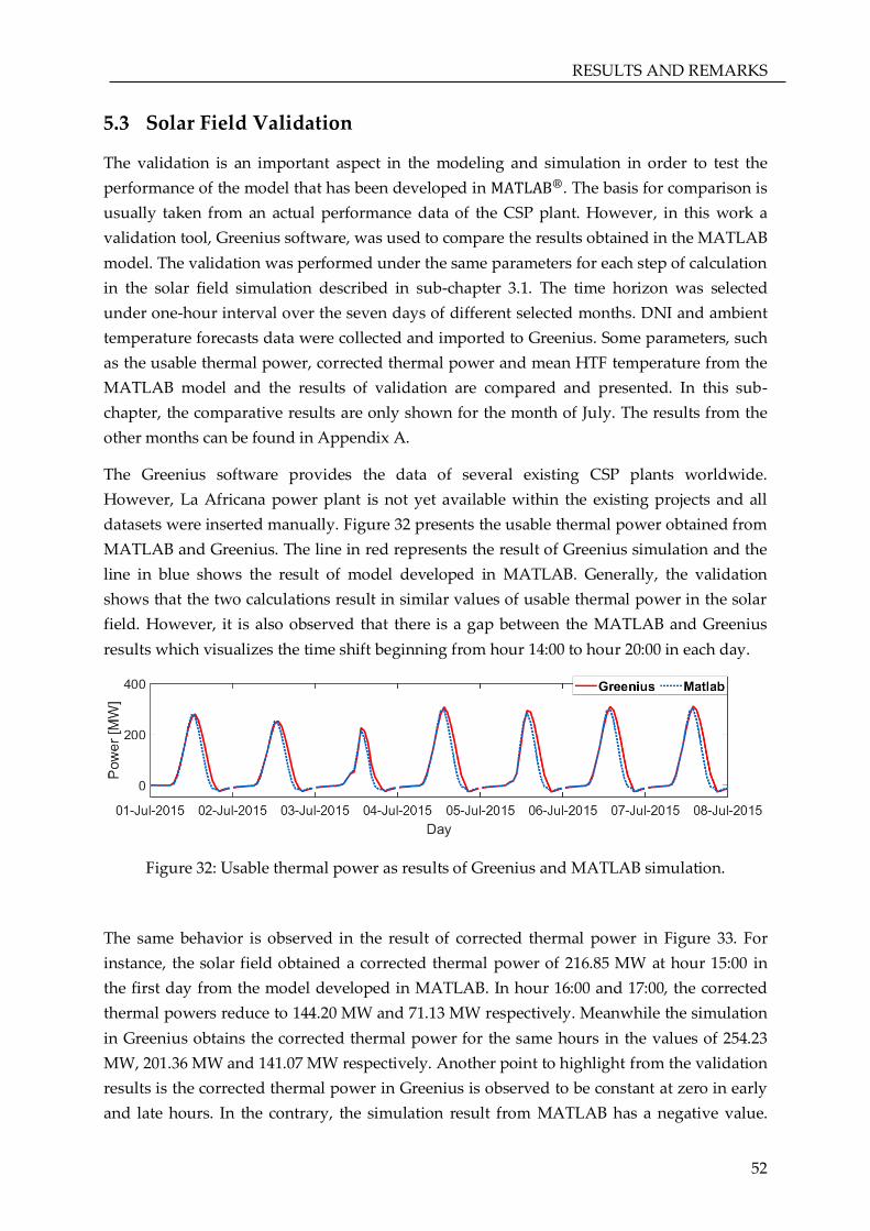
RESULTS AND REMARKS

52

Solar Field Validation

The validation is an important aspect in the modeling and simulation in order to test the

performance of the model that has been developed in MATLAB®. The basis for comparison is

usually taken from an actual performance data of the CSP plant. However, in this work a

validation tool, Greenius software, was used to compare the results obtained in the MATLAB

model. The validation was performed under the same parameters for each step of calculation

in the solar field simulation described in sub-chapter 3.1. The time horizon was selected

under one-hour interval over the seven days of different selected months. DNI and ambient

temperature forecasts data were collected and imported to Greenius. Some parameters, such

as the usable thermal power, corrected thermal power and mean HTF temperature from the

MATLAB model and the results of validation are compared and presented. In this sub-

chapter, the comparative results are only shown for the month of July. The results from the

other months can be found in Appendix A.

The Greenius software provides the data of several existing CSP plants worldwide.

However, La Africana power plant is not yet available within the existing projects and all

datasets were inserted manually. Figure 32 presents the usable thermal power obtained from

MATLAB and Greenius. The line in red represents the result of Greenius simulation and the

line in blue shows the result of model developed in MATLAB. Generally, the validation

shows that the two calculations result in similar values of usable thermal power in the solar

field. However, it is also observed that there is a gap between the MATLAB and Greenius

results which visualizes the time shift beginning from hour 14:00 to hour 20:00 in each day.

Figure 32: Usable thermal power as results of Greenius and MATLAB simulation.

The same behavior is observed in the result of corrected thermal power in Figure 33. For

instance, the solar field obtained a corrected thermal power of 216.85 MW at hour 15:00 in

the first day from the model developed in MATLAB. In hour 16:00 and 17:00, the corrected

thermal powers reduce to 144.20 MW and 71.13 MW respectively. Meanwhile the simulation

in Greenius obtains the corrected thermal power for the same hours in the values of 254.23

MW, 201.36 MW and 141.07 MW respectively. Another point to highlight from the validation

results is the corrected thermal power in Greenius is observed to be constant at zero in early

and late hours. In the contrary, the simulation result from MATLAB has a negative value.

RESULTS AND REMARKS

53

The analysis found that Greenius considers that the use of auxiliary electrical heater to

supply thermal energy when direct irradiance is not available.

Figure 33: Corrected thermal power as results of Greenius and MATLAB simulation.

The last parameter to observe in the validation is the average temperature of heat transfer

fluid presented in Figure 34. Similarly, to the usable and corrected thermal power, the time

shift is also seen in the temperature. At hour 19:00 on the first day, mean temperature of HTF

reaches 317.43 oC in MATLAB simulation. It is followed by a reduction of temperature until

it falls to 284.37 oC in the next hour. Meanwhile, the mean temperatures obtained from the

simulation in Greenius are 340.76 oC and 321.68 oC respectively for the same hours.

Figure 34: Average HTF temperature as results of Greenius and MATLAB simulation.

In general, the time shift is observed in the three parameters: usable thermal power,

corrected thermal power and mean HTF temperature. An analysis of this behavior has been

conducted by comparing the parameters defined in the solar field simulation that is

described in sub-chapter 3.1 for the model developed in MATLAB with the Greenius. Figure

35 shows the parameter observed to be the cause of shifting is the incidence angle. The

model in MATLAB calculates the incidence angle as a function of several variables

represented in (4) and (5). Each of the steps is calculated thoroughly, while the use of

equation in Greenius model is not available for a detailed observation and study.

RESULTS AND REMARKS

54

Figure 35: Incidence angle as results of Greenius and MATLAB simulation.

Dispatch Strategies Implementation

In order to evaluate the reaction of the rules, a specific set of design and control parameters

were selected according to the characteristics of an existing power plant as defined in Table

2. Moreover, the two days forecast horizon is selected because of the probability to bring

financial benefits compared to one-day forecast in the simulation [33]. The electricity price

profile is an hourly-based forecast of the Spanish electricity market, obtained from a publicly

available database [37]. In the following sections, the analysis of basic rules and optimization

rules implementation are presented. The simulation was performed for seven days of the

selected months (January, April, July and October) with two days optimization for both solar

and storage driven strategies. However, in this section only the results of the first, second

and third day are presented. Moreover, the results shown are only for the month of July

because process flows in the other months are the same.

5.4.1 Solar Driven Strategy Analysis

The basic rules in solar driven strategy maneuver the thermal outflow from the solar field to

fulfill the maximum load of the power block, neglecting the hourly electricity price values of

the 48 hours shown in Figure 36. The thermal outflow in the system is presented in Figure

37a. The bars in blue represent the corrected thermal power that behaves as the solar field

thermal output. In the solar driven strategy, the delivery of thermal energy from the solar

field to the power block at its maximum permissible capacity is of high priority in order to

produce electricity as soon as possible. The bars in orange color show the thermal power

input sent to the power block by the solar field. Figure 37b shows the level of thermal energy

in the storage. In the initial time step, TES has an available thermal energy of 200 MWh.

Furthermore, the solar field can possibly dump thermal energy if the power block and

storage are in full capacity or the thermal outflow exceeds the designed conditions in both

equipments. The dumped energy is presented in Figure 37c.

In order to understand the process flow, an example is taken from hour 13:00 of the first day.

Thermal power output from the solar field is obtained at 276 MW. It is immediately

transferred to the power block. As the thermal power value is above the maximum input

RESULTS AND REMARKS

55

power of power block at 133.67 MW (the limit is shown by the horizontal blue line), it is

possible to send the maximum thermal energy for electricity production. The excess thermal

energy is calculated from the subtraction of the two parameters and distributed to the

thermal storage. In hour 12:00, the storage has a capacity of 293.4 MWh, far below the

maximum design capacity at 940 MWh. The excess thermal power that cannot be

accommodated by the power block is about 142.33 MW. Considering the maximum storage

charge power of 116 MW, the storage can only store at this boundary condition and the

storage level is updated to 409.4 MWh at hour 13:00. Thus, there is thermal energy accounted

for 26.33 MWh that are dumped by the solar field.

Figure 36: Price forecasts data for day 1 and day 2 in July 2015.

(a)

(b)

RESULTS AND REMARKS

56

(c)


thermal flows in the systems (a), TES level (b) and solar field dumped energy (c).

Dumping of thermal energy is associated with the loss of financial income for the CSP plant.

In addition, the wasted thermal energy could possibly be used for deliverable during periods

of insufficient thermal production if it could be stored in TES. Therefore, the optimization

rules were applied into the result of basic rules. The optimization rules aim to plan the

delivery of electricity during high price times in order to obtain improved values from the

financial revenues.

In Figure 38, the algorithm evaluates the condition of thermal production in the power plant

according to the electricity price in decreasing sequence. The electricity price forecast in

Figure 36 from the Iberian market is re-ordered in the decreasing sequence and it is

represented in Figure 38a. It is obtained that the highest price reaches 70.69 €/MWh at 12:00

on the second day. The power block is expected to produce the maximum design electricity

output at this hour in order to achieve the maximum financial benefit from the production.

The condition in hour 12:00 has been met already by the solar driven basic rule and the

optimization rule proceeds to the second-best price at hour 11:00 also in the second day. It is

observed that thermal input to the power block obtained from the simulation following the

basic rules is still below the maximum design value, at 109 MW. The algorithm reacts to this

fact and discharge the storage on the amount remained to fulfill the maximum input of the

power block. It respects the maximum thermal discharge limitation as well as the minimum

TES capacity of 18.8 MWh which must be maintained from hour 11:00 until hour 24:00 on the

second day. It means that if there is a time step from hour 11:00 onwards in the second day

that cannot meet the minimum storage capacity after the storage discharge, the algorithms

will not execute the storage discharge.

Furthermore, throughout the optimization process, the algorithms also detect the time steps

where thermal energy could be possibly dumped and behaves towards this by storing it in

the TES, with respect to the maximum charge power and maximum storage capacity. The

processes are performed sequentially until the design and control parameters of the storage

and PB become the boundary of the executions. In the end, it is obtained in the first and

RESULTS AND REMARKS

57

second day of simulation that thermal energy dumped after the implementation of

optimization rules is at zero level.

(a)

(b)

(c)

(d)


forecast for day 1 and 2 in July 2015 in a decreasing sequence (a), thermal flows in the

systems (b), TES level (c) and solar field dumped energy (d).

RESULTS AND REMARKS

58

The second simulation for the solar driven strategy was performed for the second and third

day. The electricity price forecast for these days is represented in Figure 39. The

implementation was repeated on the second day in order to obtain a better plan of electricity

delivery with consideration of prices and thermal power in the following day. The TES level

of the first hour is taken from the last hour (hour 24:00) of the first day. Thermal energy

stored in TES at this hour is 537.3 MWh as shown in Figure 38c.

In the second day, the solar field produces thermal power at hour 11:00 for an amount of

109.5 MW as visualized by an orange colored bar in Figure 40a. This power is fully

transferred to the power block represented in blue bar in the same figure. The storage level

remains constant at its value as shown in Figure 40b. In the next hour, which is hour 12:00 in

the noon, the solar field produces a large amount of thermal power. It accounts of a total

202.1 MW thermal power with only 133.67 MW can be accepted by the power block as the

input power. An excess thermal power is directed to the TES with an amount of 68.43 MW

and the storage level increases to 605.73 MWh. This adjustment can be seen in Figure 40b at

hour 12:00. The process continues until the last hour of the third day. It is observed that there

is partial thermal energy dumped from the solar field in hour 13:00 in the second day which

is due to the unmet charge power with the limitation. Moreover, TES finally reaches the

maximum capacity at hour 14:00 on the third day. This results in high wasted thermal energy

at hour 14:00 and 15:00 which is represented in Figure 40c because the excessive heat can no

longer be stored in TES.

Figure 39: Price forecasts data for day 2 and day 3 in July 2015.

(a)

RESULTS AND REMARKS

59

(b)

(c)


thermal flows in the systems (a), TES level (b) and solar field dumped energy (c).

From the results obtained in the implementation of basic rules for the second and third day,

the optimization was performed. The forecast of electricity price is re-arranged in descending

order which is shown in Figure 41a. The optimization works as explained previously and the

results are shown in the remaining Figure 41.

(a)

RESULTS AND REMARKS

60

(b)

(c)

(d)


forecast in a decreasing sequence (a) thermal flows in the systems (b), TES level (c) and solar

field dumped energy (d).

5.4.2 Storage Driven Strategy Analysis

In the storage driven strategy, solar field thermal outflow is prioritized to be stored in TES

system until the maximum capacity of the storage is reached. The unloaded SF thermal

output shall not be wasted and thus, it is sent to the power block to directly generate

electricity. Due to a large production in the solar field, sometimes thermal energy cannot be

accommodated by the two units and it requires dumping of thermal energy. As seen in

Figure 42a, the solar field thermal output powers are presented by the blue bars. Thermal

output is transferred to TES that has an initial thermal energy level at 200 MWh shown in

RESULTS AND REMARKS

61

Figure 42b. At hour 11:00 on the first day of July, the solar field produces 131 MW of thermal

power. Being the first priority, the whole thermal power is attempted to be transferred to the

storage. However, due to the system boundary from the maximum storage charge power,

TES can only accept 116 MW and the remaining thermal power is defined as the excess SF

thermal outflow presented in Figure 42c. It accounts to an amount of 15.02 MW, which is

transferred to the power block. The process continues following the same orders of thermal

flow and it gives an accumulative thermal energy inside the storage which increases every

hour.

At hour 17:00 on the same day, the solar field has a total of 71.14 MW of thermal power. The

storage level in an hour before already reaches 896 MW. By means, TES can only store 44

MW as it is the available capacity for thermal energy. The remaining thermal power of 27.14

MW is the excess solar field outflow to be sent to the power block. In the next hours,

beginning from hour 18 on the first day until hour 24:00 on the second day, the storage is full

and incapable to store more thermal energy. Thus, it results in a direct distribution of

thermal power from the solar field to the power block. When the power block reaches its

maximum input power of 133.67 MW, thermal energy is wasted from the solar field

presented in Figure 42d. Thermal energy wasted from the solar field are observed at hour

13:00 and 14:00 on the first day, as well as from hour 12:00 to 15:00 on the second day in July

2015.

(a)

(b)

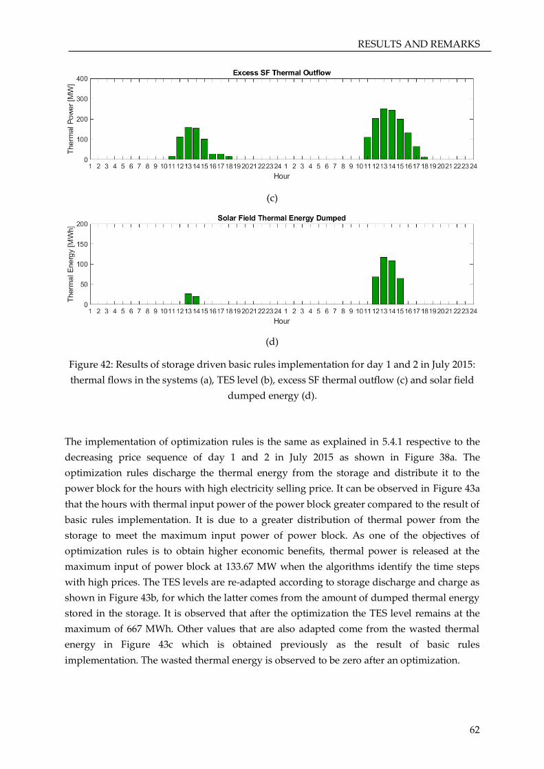
RESULTS AND REMARKS

62

(c)

(d)

Figure 42: Results of storage driven basic rules implementation for day 1 and 2 in July 2015:

thermal flows in the systems (a), TES level (b), excess SF thermal outflow (c) and solar field

dumped energy (d).

The implementation of optimization rules is the same as explained in 5.4.1 respective to the

decreasing price sequence of day 1 and 2 in July 2015 as shown in Figure 38a. The

optimization rules discharge the thermal energy from the storage and distribute it to the

power block for the hours with high electricity selling price. It can be observed in Figure 43a

that the hours with thermal input power of the power block greater compared to the result of

basic rules implementation. It is due to a greater distribution of thermal power from the

storage to meet the maximum input power of power block. As one of the objectives of

optimization rules is to obtain higher economic benefits, thermal power is released at the

maximum input of power block at 133.67 MW when the algorithms identify the time steps

with high prices. The TES levels are re-adapted according to storage discharge and charge as

shown in Figure 43b, for which the latter comes from the amount of dumped thermal energy

stored in the storage. It is observed that after the optimization the TES level remains at the

maximum of 667 MWh. Other values that are also adapted come from the wasted thermal

energy in Figure 43c which is obtained previously as the result of basic rules

implementation. The wasted thermal energy is observed to be zero after an optimization.

RESULTS AND REMARKS

63

(a)

(b)

(c)


TES level (b) and solar field dumped energy (c).

The second simulation was conducted for the second and third day of July. In the first hour

of the second day, TES has an available stored thermal energy of 667 MWh, that is obtained

from hour 24:00 of the first day. It is seen in Figure 44b that the TES level remains constant

until hour 10:00 because the solar field does not produce thermal energy. An hour later, at

11:00, solar field produces 109.5 MW thermal power to be distributed to the storage. The

level of thermal energy increases to 776.6 MWh because the SF outflow is below the

maximum charge power limitation. Thus, all thermal power is stored in TES. However, a

different manner is observed at hour 12:00 where the solar field produces 202.1 MW of

thermal power. In fact, the storage is capable to store 163.4 MWh of thermal energy, but the

storage has the maximum charge power limitation of 116 MW. Hence, the violation of charge

RESULTS AND REMARKS

64

power is impossible and the solar field thermal output is stored as the same amount of the

designed maximum charge power. The excess thermal power is presented in Figure 44c. It is

transferred to the power block shown in Figure 44a as the bars in orange color. At hour 13:00

of the first day, the solar field produces an amount of 251.1 MW as shown in Figure 44a in

blue bar, while the storage can only store 47.4 MWh of thermal energy. Hence, the remaining

203.6 MW of thermal power is distributed to the power block until it is full. The maximum

limitation is reached at 133.67 and the excess thermal energy is dumped from the solar field,

with a total amount of 69.96 MWh as seen in Figure 44d. In the next hours, the storage is no

longer capable of receiving thermal energy. Thermal power outflow from the solar field are

counted as the excess heat and transferred directly to the power block.

(a)

(b)

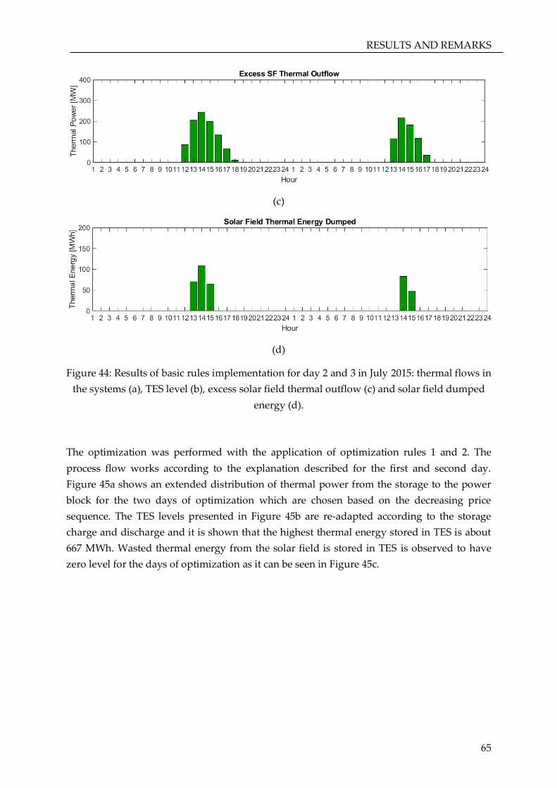
RESULTS AND REMARKS

65

(c)

(d)

Figure 44: Results of basic rules implementation for day 2 and 3 in July 2015: thermal flows in

the systems (a), TES level (b), excess solar field thermal outflow (c) and solar field dumped

energy (d).

The optimization was performed with the application of optimization rules 1 and 2. The

process flow works according to the explanation described for the first and second day.

Figure 45a shows an extended distribution of thermal power from the storage to the power

block for the two days of optimization which are chosen based on the decreasing price

sequence. The TES levels presented in Figure 45b are re-adapted according to the storage

charge and discharge and it is shown that the highest thermal energy stored in TES is about

667 MWh. Wasted thermal energy from the solar field is stored in TES is observed to have

zero level for the days of optimization as it can be seen in Figure 45c.

RESULTS AND REMARKS

66

(a)

(b)

(c)


TES level (b) and solar field dumped energy (c).

Power Block Electrical Output

Thermal power is delivered to the power cycle system from the solar field or the TES system

for the production of electricity in the steam turbine and generator. The parasitic electricity

consumption of the pumps used for the molten salts is not considered in the simulation. The

same is applied for the solar field parasitic, such as the HTF main pumps, HTF circulation

pumps, tracking, and the auxiliary electrical heaters. Moreover, parasitic consumption that

comes from the power block sub-system is also not considered in the model. Therefore, the

produced electricity can be defined as the gross electricity output from the power system. In

RESULTS AND REMARKS

67

the following sections, an hourly of electrical output produced in the power block from the

application of basic rules and the optimization are compared for the two dispatch strategies:

solar driven and storage driven. Furthermore, the accumulative results for each of the

months are analyzed and discussed.

The calculation of electrical output from the power is based on the use of lookup table that

can be found in Appendix B. It consists of three parameters: thermal input power, ambient

temperature and relative ambient humidity. Among these parameters, ambient humidity is a

selected one fixed value of 60% obtained as an average value for the location of La Africana

CSP plant. These attributes were used to perform the interpolation of a given data of

thermal power input at every time step.

5.5.1 Basic vs. Optimized Solar Driven Strategy

Figure 46 shows the electricity generated in MWe for the seven days of the selected months

with the solar driven strategy. It can be observed that the electricity production is limited to

the day times once the basic rules are applied. In the nights, the power block does not

operate, as the supply of thermal power from the solar field is not available. In general, the

power block reaches the peak electrical output production in the middle of the day, from

12:00 to 15:00. For example, in the seventh day of January, the highest electricity generation is

obtained at hour 12:00 for an amount of 54.32 MWe. Meanwhile, in April, July and October

the power block electrical outputs reach the peak value of 53.51 MWe, 52.43 MWe and 53.42

MWe respectively.

Figure 46: Power block electrical output with the implementation of basic rules.

The electrical output is extended to longer hours in the days once the optimization rules are

applied, as shown in Figure 47. The figure shows the result of optimization for the solar

driven strategy. Unlike the result shown in the previous figure, the electricity generation also

takes place during the night times when irradiance is not available. Thermal power is

supplied from the storage for the hours with high electricity sale prices.

RESULTS AND REMARKS

68

Figure 47: Power block electrical output with the implementation of optimization rules.

Accumulative results of power block input power, dumped thermal energy, electrical output

and the financial revenues are calculated for each of the months. Figure 48 represents the

overall results from the implementation of basic and optimization rules under the solar

driven model for the selected four months of simulation. The evaluations can be realized

from the electricity production as well as the economical contribution in the application to

obtain the highest financial revenue for the CSP plant. It is seen that July has the highest

values compared to the other months, with thermal power input of 6.1 GW and 9.04 GW

thermal under basic and optimized conditions, respectively as shown in Figure 48a. The

electrical outputs are produced for about 2.32 GW and 3.47 GW electricity, respectively. The

financial income obtained from the electricity sale is at 143 thousand Euro and increases to

217 thousand Euro with the optimization rules which represented in Figure 48b. The orders

of the results from the highest to the lowest are followed by October, April and January

respectively. The efficiency of power block can be greatly observed in Figure 48a which

shows PB thermal input power and electrical output for the basic and optimized conditions.

The electrical output is about 39% of the thermal input power.

In general, the simulated parabolic CSP plant with a solar driven dispatch strategy is capable

to generate a total of 9.7 GWh of electricity for all the months with the implementation of

dispatch optimization rules. This is 54% higher compared to the basic rules application,

which only produces 6.3 GWh of electricity for the selected four months of simulation. With

the precise values of power block electricity output, a financial contribution of the rules can

be assessed. The dispatch optimization rules contribute to increase the revenue from selling

the electricity for an average of 65% when compared to the revenue obtained from the

application of basic rules. Initially, the basic rules can only generate a total of 322 thousand

Euro financial revenue, while with the optimization rules, the income value is quantified to

increase significantly to 530 thousand Euro. Furthermore, the solar field initially dumps 4.3

GWh of thermal energy due to an insufficient storage capacity in the TES system. With the

dispatch optimization rules, the dumped energy is completely reduced. It is important to

remember that these values are theoretical, considering that the calculations are based on the

PB gross output and does not consider PB ramp up procedures.

RESULTS AND REMARKS

69

(a)

(b)

RESULTS AND REMARKS

70

(c)

Figure 48: Overall results of basic and dispatch optimization rules considering the solar

driven approach: comparison between PB thermal power input and electricity generation (a),

financial income (b) and dumped thermal energy (c).

5.5.2 Basic vs. Optimized Storage Driven Strategy

The implementation of basic rules in storage driven strategy can be observed in PB output

term in Figure 49. Similarly to the one in solar driven strategy, electricity production is

limited to the hours where the solar field produces thermal energy once only the basic rules

are applied. The electricity can only be generated when there is an excess of thermal power

transferred to the power block. This excess thermal power is obtained because the storage

has met the charging power limitation or the maximum capacity. Figure 50 shows the

electricity generation from the application of optimization rules. Compared to the result of

basic rules, the electrical output is expanded to the hours where the electricity prices are

high. Thermal storage discharge thermal energy to the power block and maximize the value

to reach the maximum input power of PB. However, it has to work according to the

discharge limitation and minimum capacity. It can be observed that the electrical output is

also obtained at night times, where usually the demand from consumers are high and

relevantly increase the price.

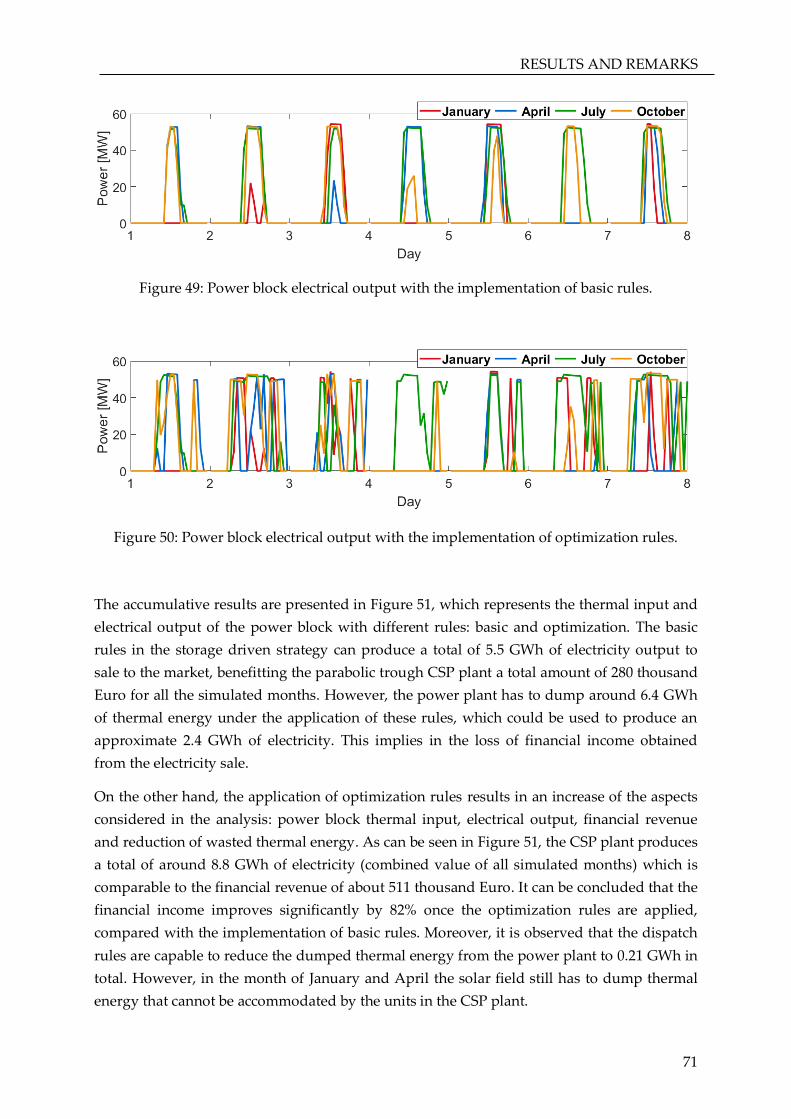
RESULTS AND REMARKS

71

Figure 49: Power block electrical output with the implementation of basic rules.

Figure 50: Power block electrical output with the implementation of optimization rules.

The accumulative results are presented in Figure 51, which represents the thermal input and

electrical output of the power block with different rules: basic and optimization. The basic

rules in the storage driven strategy can produce a total of 5.5 GWh of electricity output to

sale to the market, benefitting the parabolic trough CSP plant a total amount of 280 thousand

Euro for all the simulated months. However, the power plant has to dump around 6.4 GWh

of thermal energy under the application of these rules, which could be used to produce an

approximate 2.4 GWh of electricity. This implies in the loss of financial income obtained

from the electricity sale.

On the other hand, the application of optimization rules results in an increase of the aspects

considered in the analysis: power block thermal input, electrical output, financial revenue

and reduction of wasted thermal energy. As can be seen in Figure 51, the CSP plant produces

a total of around 8.8 GWh of electricity (combined value of all simulated months) which is

comparable to the financial revenue of about 511 thousand Euro. It can be concluded that the

financial income improves significantly by 82% once the optimization rules are applied,

compared with the implementation of basic rules. Moreover, it is observed that the dispatch

rules are capable to reduce the dumped thermal energy from the power plant to 0.21 GWh in

total. However, in the month of January and April the solar field still has to dump thermal

energy that cannot be accommodated by the units in the CSP plant.

RESULTS AND REMARKS

72

Compared with the application of both rules in the solar driven strategy, the storage driven

generates lower economic benefits. It is due to the thermal energy stored in TES is limited by

the design condition of maximum discharging storage power. Moreover, dumping of

thermal energy remains because the TES is only capable to store 940 MWh with a maximum

charge power limitation of 116 MW.

(a)

(b)

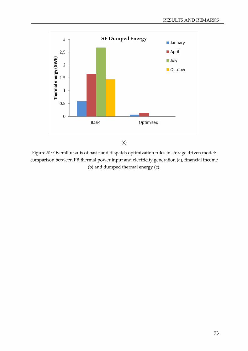
RESULTS AND REMARKS

73

(c)

Figure 51: Overall results of basic and dispatch optimization rules in storage driven model:

comparison between PB thermal power input and electricity generation (a), financial income

(b) and dumped thermal energy (c).

SUMMARY AND OUTLOOK

74

6 SUMMARY AND OUTLOOK

Details of the simulation model of the parabolic trough CSP plant have been presented

covering the solar field model development and validation. The simulation was performed

using a reference data from La Africana CSP plant that is equipped with parabolic trough

collectors, two-tank indirect thermal storage and the power block with Rankine cycle. Two

types of working fluids are used, with the first one is thermal oil behaves as the heat transfer

fluid circulating in the solar field. Another one, molten salt, is used as the working fluid in

TES. The simulation was performed for seven days from different selected months: January,

April, July and October of year 2015, to obtain the final thermal power output of the solar

field, which is defined as the corrected thermal power.

The validation of solar field model was performed with Greenius. Three major parameters

were analyzed: the usable thermal power, corrected thermal power and mean HTF

temperatures. The results show that the model developed in MATLAB is similar to the

simulation in Greenius, which it can be concluded that the model works properly. The gap

between the two models was observed in the late hours where there is a time shift. It is

analyzed to be the difference from result of incidence angle determination which can be a

potential improvement in the future.

In the next step, the corrected thermal power was used as an important input parameter for

the development of dispatch strategies. Two schemes were presented based on the thermal

distribution: the solar driven and storage driven strategies. Under them, the basic rules and

optimization rules were performed. The first one distributes the thermal output power from

the solar field to the prioritized unit. The optimization rules, on the other hand, re-arrange

the electricity distribution based on decreasing high price times. These rules were

implemented after the basic rules. The results show that optimization rules prove to increase

the electrical output generated from the power block as well as improve the financial income

from the electricity sales. The electricity production increases from 6.3 GWh in basic rules to

9.7 GWh in optimization rules application in solar driven approach and from 5.5 GWh to 8.8

GWh in storage driven. As for the financial improvement, the value increases from 322

thousand Euro to 530 thousand Euro from the basic to optimization rules in solar driven and

from 280 thousand Euro to 511 thousand Euro in storage driven approach. The optimization

also proves to reduce dumped thermal energy significantly in both approaches. More

importantly, the implementation of optimization rules based on the solar driven strategy is

seen to bring a higher benefits for the power plant compared to the storage driven strategy. It

is due to the maximum discharge power limitation in TES that is below the power block

maximum design input power.

From the models developed and the results obtained here, some aspects were identified for

further work. First of all, the developed algorithms serve a simple understanding with high

computational speed for an adaptation with different weather forecasts data. Therefore, the

extension of function with an annual simulation is possible in order to give broader result

SUMMARY AND OUTLOOK

75

and comprehensive analysis of the performance of parabolic trough CSP plant operation.

Another important aspect that could be further developed is related to a comprehensive

design of the sub-systems, majorly in the power block. The design of the solar field has

complied with the type of operating system. As the focus of the work relies on the

development of dispatch strategies, some simplifications are made in the modeling of the

power block and it can be extended for further studies.

REFERENCES

76

7 REFERENCES

[1] D. Connolly, "The Integration of Fluctuating Renewable Energy Using Energy Storage,"

The University of Limerick, 2010.

[2] Y. Wang, S. Lou, Y. Wu and S. Wang, "Co-allocation of solar field and thermal energy

storage for CSP plants in wind-integrated power system," IET Renewable Power

Generation, vol. 12, no. 14, pp. 1668-1674, 2019.

[3] H. Gong, V. Rallabandi, D. M. Ionel, D. Colliver, S. Duerr and C. Ababei, "Net Zero

Energy Houses with Dispatchable Solar PV Power Supported by Electric Water Heater

and Battery Energy Storage," IEEE Energy Conversion Congress and Exposition (ECCE), pp.

2498-2503, 2018.

[4] R. Dominguez, L. Baringo and A. J. Conejo, "Optimal offering strategy for a

concentrating solar power plant," Applied Energy, 98, p. 316–325, 2012.

[5] H. I. Pousinho, J. Contreras, P. Pinson and V. F. Mendes, "Pousinho, H. M. I., Contreras,

J., Pinson, P., & Mendes, V. M. F. (2015). Robust optimisation for self-scheduling and

bidding strategies of hybrid CSP–fossil power plants," International Journal of Electrical

Power & Energy Systems, 67, p. 639–650, 2015.

[6] M. J. Wagner, A. M. Newman, W. T. Hamilton and R. J. Braun, "Optimized dispatch in a

first-principles concentrating solar power production model," Applied Energy, 203, pp.

959-971, 2017.

[7] A. C. d. A. Burghi, T. Hirsch and R. Pitz-Paal, "FRED: The Flexible Renewable Energy

System Dispatch Optimizer," ASME. J. Sol. Energy Eng. October 2019; 141(5): 051009, p.

141(5): 051009, 2019.

[8] "Institutes and Facilities," Deutsches Zentrum für Luft-und Raumfahrt, [Online].

Available: https://www.dlr.de/EN/organisation-dlr/dlr/institutes-and-facilities.html.

[Accessed 20 October 2019].

[9] "About us: DLR Institute of Solar Research," Deutsches Zentrum für Luft-und

Raumfahrt, [Online]. Available: https://www.dlr.de/sf/en/desktopdefault.aspx/tabid-

REFERENCES

77

7128/15166_read-37505/). [Accessed 20 October 2019].

[10] "Home: Research and Development: Line Focus Systems," Deutsches Zentrum für Luft-

und Raumfahrt, [Online]. Available:

https://www.dlr.de/sf/en/desktopdefault.aspx/tabid-7088/18782_read-43608/. [Accessed

20 October 2019].

[11] A. Giostri, M. Binotti, M. Astolfi, P. Silva, E. Macchi and G. Manzolini, "Comparison of

Different Solar Plants Based on Parabolic Trough Technology," Solar Energy, vol. 86, no.

5, p. 1208–1221, 2012.

[12] S. Suojanen, "Development of Concentrated Solar Power and Conventional Power Plant

Hybrids," Tampere University of Technology, 2016.

[13] H. G. Jin and H. Hong, "Hybridization of concentrating solar power (CSP) with fossil

fuel power plants," in Concentrating Solar Power Technology, Principles, Developments and

Applications, Woodhead Publishing Series in Energy, 2012, pp. 395-420.

[14] R. Guédez, "A Techno-Economic Framework for the Analysis of Concentrating Solar

Power Plants with Storage," diva2:956167, Stockholm, 2016.

[15] "Technology Roadmap: Solar Thermal Electricity," International Energy Agency, Paris,

2014.

[16] M. Günther , "Advanced CSP Teaching Materials: Chapter 6 Linear Fresnel Technology".

[17] D. Barlev, R. Vidu and P. Stroeve, "Innovation in Concentrated Solar Power," Solar

Energy Materials & Solar Cells, vol. 95, pp. 2703-2725, 2011.

[18] W. B. Stine and M. Geyer, "Chapter 8. Concentrator Optics," in Power from The Sun, 2001.

[19] M. Günther, M. Joemann and S. Csambor, "Advanced CSP Teaching Materials: Chapter

5 Parabolic Trough Technology".

[20] E. Z. Moya, "Parabolic-trough concentrating solar power (CSP) systems," in

Concentrating Solar Power Technology, Principle, Developments and Applications, Woodhead

Publishing Limited, 2012, pp. 197-239.

REFERENCES

78

[21] A. Mwesigye, T. B. Ochende, W. G. Le Roux and J. P. Meyer, "Thermal and

Thermodynamic Analysis of a Parabolic Trough Receiver at Different Cocentration

Ratios and Rim Angles," in 10th International Conference on Heat Transfer, Fluid Mechanics

and Thermodynamics, Orlando, 2014.

[22] S. A. Kalogirou, "Chapter 10 - Solar Thermal Power Systems," in Solar Energy

Engineering, Processes and Systems, 2 ed., Elsevier, 2014, pp. 541-581.

[23] I. L. Garcia, J. L. Alvarez and D. Blanco, "Performance Model for Parabolic Trough Solar

Thermal Power Plants with Thermal Storage: Comparison to Operating Plant Data,"

Solar Energy, vol. 85, pp. 2443-2460, 2011.

[24] M. Blaco and S. Miller, "Introduction to concentrating," in Advances in Concentrating Solar

Thermal Research and Technology, Woodhead Publishing Limited, 2017, pp. 3-25.

[25] L. Heller, "Literature Review on Heat Transfer Fluids and Thermal Energy Storage

Systems in CSP Plants, STERG Report," 2013.

[26] J. A. Duffie and W. A. Beckman, Solar Engineering of Thermal Processes, 2nd edition,

New York: John Wily & Sons, Inc, 1991.

[27] S. Kalaiselvam and R. Parameshwaran, "Sensible Thermal Energy Storage," in Thermal

Energy Storage for Sustainability, Elsevier, 2014, pp. 65-82.

[28] M. Medrano, A. Gil, I. Martorell, X. Potau and L. F. Cabeza, "State of the art on high-

temperature thermal energy storage for power generation. Part 2—Case studies,"

Renewable and Sustainable Energy Reviews, vol. 14, no. 1, pp. 56-72, 2010.

[29] D. Y. Goswami, F. Kreith and J. F. Kreider, Principles of Solar Engineering 2nd Edition,

Philadelphia: Taylor & Francis, 2000.

[30] "Solar Position and Intensity," NREL: U.S Department of Energy, [Online]. Available:

https://www.nrel.gov/grid/solar-resource/solpos.html. [Accessed 09 09 2019].

[31] D. Z. f. L.-u. Raumfahrt, "Greenius: Green Energy System Analysis Manual," DLR Solar

Research, Cologne, 2018.

REFERENCES

79

[32] T. Hirsch , J. Dersch, T. Fluri, S. Giuliano, R. Meyer, E. Yildiz, J. G. Barberena, F. H.

Diethelm, N. Schmidt and M. Seitz, "SolarPACES Guideline for Bankable STE Yield

Assessment," IEA Technology Collaboration Programme SolarPACES, Tabernas, 2017.

[33] M. Wittmann, M. Eck, R. Pitz-Paal and H. M. Steinhagen, "Methodology for optimized

operation strategies of solar thermal power plants with integrated heat storage," Solar

Energy, vol. 85, pp. 653-659, 2011.

[34] B. Kraas, M. S. Homscheidt and R. Madlener, "Economic merits of a state-of-the-art

concentrating solar power forecasting system for participation in the Spanish electricity

market," Solar Energy, vol. 93, pp. 244-255, 2013.

[35] "EarthSky," 23 September 2019. [Online]. Available: https://earthsky.org/earth/can-you-

explain-why-earth-has-four-seasons. [Accessed 20 December 2019].

[36] J. Lansdberg and P. Sands, "Weather and Energy Balance," Terrestrial Ecology, vol. 4, pp.

13-48, 2011.

[37] "Sistema de Información del Operador del Sistema (e·sios)," Red Eléctrica de España,

[Online]. Available: https://www.esios.ree.es/en/analysis/805?vis=1&start_date=23-09-

2019T00%3A00&end_date=23-09-2019T23%3A00&compare_start_date=22-09-

2019T00%3A00&groupby=hour. [Accessed 1 10 2019].

APPENDIX

80

8 APPENDIX

A. Results of Solar Field Validations

• The month of January

Figure 52: Usable thermal power in January 2015.

Figure 53: Corrected thermal power in January 2015.

Figure 54: Actual HTF Temperature in January 2015.

APPENDIX

81

• The month of April

Figure 55: Usable thermal power in April 2015.

Figure 56: Corrected thermal power in April 2015.

Figure 57: Actual HTF Temperature in April 2015.

APPENDIX

82

• The month of October

Figure 58: Usable thermal power in October 2015.

Figure 59: Corrected thermal power in October 2015.

Figure 60: Actual HTF Temperature in October 2015.

APPENDIX

83

B. Power block lookup table


conditions part 1

Thermal input range

[kW]

0 20,391 20,392 33,987 50,980 67,461 78,791

Amb.

humidity

Amb.

Temp

[oC]

Electricity output [kW]

0 0 0 0 8,005.4 12,877.9 18,537.1 24,101.1 29,246.3

0 15 0 0 8,005.4 12,877.9 18,537.1 24,101.1 29,151.0

0 30 0 0 8,005.4 12,877.9 18,509.7 23,795.6 28,641.5

0 45 0 0 8,005.4 12,783.6 18,166.4 23,393.2 28,211.5

20 0 0 0 8,005.4 12,877.9 18,537.1 24,101.1 29,246.3

20 15 0 0 8,005.4 12,877.9 18,537.1 24,101.1 28,980.6

20 30 0 0 6,211.7 11,080.0 17,385.5 24,177.7 29,019.0

20 45 0 0 7,758.7 12,375.4 17,633.5 22,737.2 27,460.2

40 0 0 0 8,005.4 12,877.9 18,537.1 24,101.1 29,246.3

40 15 0 0 8,005.4 12,877.9 18,537.1 23,947.7 28,801.3

40 30 0 0 7,932.4 12,618.2 17,941.9 23,125.5 27,904.3

40 45 0 0 7,523.9 12,041.7 17,204.2 22,184.6 26,829.1

60 0 0 0 8,005.4 12,877.9 18,537.1 24,101.1 29,246.3

60 15 0 0 8,005.4 12,877.9 18,505.3 23,787.8 28,630.8

60 30 0 0 7,802.9 12,436.8 17,710.9 22,833.9 27,570.3

60 45 0 0 7,330.9 11,764.3 16,843.1 21,716.0 26,291.4

APPENDIX

84


conditions part 2

Thermal input range

[kW]

88,943 98,134 106,525 114,217 121,253 126,478 130,166 133,678

Amb.

humidity

Amb.

Temp

[oC]

Electricity output [kW]

0 0 33,823.8 38,148.5 41,929.4 45,421.8 48,669.7 51,773.8 52,907.4 55,229.0

0 15 33,427.4 37,404.5 41,130.4 44,591.3 47,811.6 51,007.4 52,136.8 54,450.4

0 30 32,878.1 36,804.0 40,497.1 43,929.2 47,123.7 50,387.6 51,512.3 53,816.5

0 45 32,411.4 36,291.2 39,953.5 43,358.1 46,527.8 49,814.9 50,966.4 53,260.6

20 0 33,823.8 38,088.9 41,847.2 45,336.2 48,581.1 51,694.6 52,827.8 55,148.5

20 15 33,243.2 37,202.7 40,917.2 44,368.0 47,579.3 50,798.0 51,925.7 54,236.0

20 30 33,242.6 37,161.2 40,843.6 44,264.1 47,405.7 49,993.0 51,441.1 52,814.4

20 45 31,631.8 35,427.2 39,030.1 42,380.6 45,501.1 48,524.2 50,013.7 52,285.1

40 0 33,823.8 37,984.2 41,737.3 45,221.9 48,462.9 51,589.0 52,721.6 55,041.3

40 15 33,049.1 36,989.8 40,692.0 44,132.0 47,333.5 50,576.1 51,701.9 54,008.3

40 30 32,092.1 35,936.7 39,574.1 42,956.0 46,105.0 49,241.8 50,574.1 52,858.6

40 45 30,970.7 34,707.2 38,238.4 41,538.4 44,612.4 47,590.9 48,836.9 51,428.5

60 0 33,823.8 37,882.3 41,630.4 45,110.5 48,347.7 51,486.1 52,618.1 54,936.5

60 15 32,864.3 36,786.8 40,477.0 43,906.2 47,098.1 50,363.0 51,486.9 53,789.4

60 30 31,745.4 35,552.4 39,163.2 42,520.9 45,647.8 48,677.1 50,149.5 52,423.7

60 45 30,403.0 34,088.5 37,552.5 40,805.7 43,836.4 46,773.2 48,001.7 50,671.4

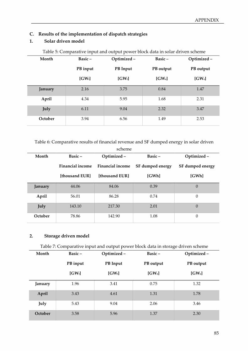
APPENDIX

85

C. Results of the implementation of dispatch strategies

1. Solar driven model

Table 5: Comparative input and output power block data in solar driven scheme

Month Basic –

PB input

[GWt]

Optimized –

PB Input

[GWt]

Basic –

PB output

[GWe]

Optimized –

PB output

[GWe]

January 2.16 3.75 0.84 1.47

April 4.34 5.95 1.68 2.31

July 6.11 9.04 2.32 3.47

October 3.94 6.56 1.49 2.53

Table 6: Comparative results of financial revenue and SF dumped energy in solar driven

scheme

Month Basic –

Financial income

[thousand EUR]

Optimized –

Financial income

[thousand EUR]

Basic –

SF dumped energy

[GWh]

Optimized –

SF dumped energy

[GWh]

January 44.06 84.06 0.39 0

April 56.01 86.28 0.74 0

July 143.10 217.30 2.01 0

October 78.86 142.90 1.08 0

2. Storage driven model

Table 7: Comparative input and output power block data in storage driven scheme

Month Basic –

PB input

[GWt]

Optimized –

PB Input

[GWt]

Basic –

PB output

[GWe]

Optimized –

PB output

[GWe]

January 1.96 3.41 0.75 1.32

April 3.43 4.61 1.31 1.78

July 5.43 9.04 2.06 3.46

October 3.58 5.96 1.37 2.30

APPENDIX

86

Table 8: Comparative results of financial revenue and SF dumped energy in storage driven

scheme

Month Basic –

Financial income

[thousand EUR]

Optimized –

Financial income

[thousand EUR]

Basic –

SF dumped energy

[GWh]

Optimized –

SF dumped energy

[GWh]

January 39.43 82.63 0.593 0.07

April 42.80 72.09 1.66 0.14

July 126.29 220.38 2.68 0

October 71.57 136.65 1.45 0

Dispatch Optimizer for Concentrated Solar Power Plants1385912/... · 2020-01-15 · Dispatch...

Documents

Transcript of Dispatch Optimizer for Concentrated Solar Power Plants1385912/... · 2020-01-15 · Dispatch...