DISORDERED FIELD PATTERNS IN A WAVEGUIDE WITH PERIODIC ...

Progress In Electromagnetics Research B, Vol. 48, 329–346, 2013

DISORDERED FIELD PATTERNS IN A WAVEGUIDEWITH PERIODIC SURFACES

Hector Perez-Aguilar1, *, Alberto Mendoza-Suarez1,Eduardo S. Tututi1, and Ivan F. Herrera-Gonzalez2

1Facultad de Ciencias Fısico-Matematicas, Universidad Michoacana deSan Nicolas de Hidalgo, Av. Francisco J. Mujica S/N 58030, Morelia,Michoacan, Mexico2Instituto de Fısica, Benemerita Universidad Autonoma de Puebla,Apartado Postal J-48, Puebla 72570, Mexico

Abstract—This paper considers an electromagnetic waveguidecomposed of two periodic, perfectly conducting, rippled surfaces. Thisperiodic system has a band structure given by a dispersion relation thatallows us characterize eigenmodes of the system. We considered thecases of both smooth and rough surfaces, using an integral numericalmethod to calculate field intensities corresponding to eigenmodes overa wide frequency range. Under certain conditions, the system presentsdisordered patterns of field intensities with smooth surfaces. Webelieve that the explanation of disordered patterns is the following:for smooth surfaces, the phenomenon of electromagnetic chaos; and forrough surfaces, the speckle phenomenon. Since it is well known thatthe surfaces of materials always have a certain degree of roughness,it can be concluded that both chaos and speckle contribute to thepresence of disordered field patterns.

1. INTRODUCTION

It is now recognized that the basic random interference phenomenonunderlying disordered patterns has close parallels in many otherbranches of physics and engineering [1]. Perhaps the earliestinvestigations of the properties of electromagnetic fields scattered fromrough surfaces were those conducted by Lord Rayleigh [2]. It is alsowell known that, as a result of the interference among the distinctrandom contributions from the scattering centers, on scale of the

Received 5 December 2012, Accepted 28 January 2013, Scheduled 30 January 2013* Corresponding author: Hector Perez-Aguilar ([email protected]).

330 Perez-Aguilar et al.

optical wavelength, the scattered field pattern appears disordered, withcertain granularity. This irregular pattern is best described by methodsof probability theory and statistics. The physical origin of the observedgranularity, now know as “laser speckle”, was quickly recognized byearly workers in the field [3, 4].

The study of the statistical properties of disordered systems is offundamental importance because it leads to phenomena such as weak(enhanced backscattering) [5] and strong (Anderson) [6] localization,intensity correlations [7], and universal conductance fluctuations [8].Furthermore, recent developments on the theory of disordered systemsbased upon nonlinear o models using supersymmetry theory [9] haveled to the recognition that the extreme diffusive limit of disorderedsystems also behaves similarly to quantum chaotic systems.

One particularly important issue in this field is the attemptto identify evidence of chaos in the transport properties of ballisticsystems. In fact, the magnetoresistance has been measured inchaotic and in regular cavities showing clearly distinctions in quantumtransport [10]. The signature of chaos in classical transport throughwaveguides has also been investigated, and shows a completelydifferent behavior on the resistivity when the system is regular orchaotic [11, 12].

This paper examines an electromagnetic waveguide composedof two periodic, perfectly conducting, rippled surfaces, taking intoaccount the cases of both smooth and rough surfaces. Thus, this papercompletes the study of the system introduced in Ref. [13]. The resultsof this study show that the system has many interesting properties.

The study of the transport properties of random systems hasconsidered that disorder in the system is usually represented byimpurities that are randomly distributed over the whole sample.However, it is worth mentioning that our system of a waveguide withsmooth rippled surfaces can present disordered field patterns; undercertain conditions, of course. This kind of systems has been thesubject of several studies in recent years due to their importance inthe design of antennas and rectangular waveguides for macroscopicsystems [14–16] and waveguides that are related to photonic crystals,as per Ref. [13]. These systems, which constitute periodic arraysof different materials with a unit cell of dimensions of the order ofthe wavelength, hold the potential to develop new technologies ofintegrated optical circuits [17].

The geometry of waveguides with smooth rippled surfaces hasbeen considered to constitute some billiard systems in order to studytheir quantum and classical transport properties [12, 18, 19]. Hence,it is important to mention that using the geometry of the proposed

Progress In Electromagnetics Research B, Vol. 48, 2013 331

system with smooth surfaces for modeling a classical waveguide,usually leads to chaotic behavior in the trajectories of the particlesthat are transported through it. Thus, this paper also considersthe manifestation of classical chaotic dynamics in the correspondingelectromagnetic system through an infinite rippled waveguide.

A disordered pattern is not enough to ensure the presence ofchaos since it is difficult to distinguish between chaotic and specklepatterns [20, 21]. However, these chaotic and speckle phenomenahave applications in various uses, such as coupling high pump powerinto chaotic double-clad EDFA’s [20], mechanical models of Chua’scircuit [22], cryptography based on chaotic systems [23], algorithmictrading [24], measurements of coherence [25], surface roughness [26],and displacement of an object [27], among others.

This paper is organized as follows: Section 2 introduces an integralmethod to calculate the field intensities of an infinite optical waveguidebased on the ideas of Ref. [28]. Section 3 shows numerical results ofdisordered patterns in a waveguide with surfaces modeled with smoothharmonic profiles. Section 4 uses another integral method to obtainsome numerical results in the case of a more realistic finite waveguidewith rough surfaces. Finally, Section 5 presents our conclusions.

2. THEORETICAL APPROACH

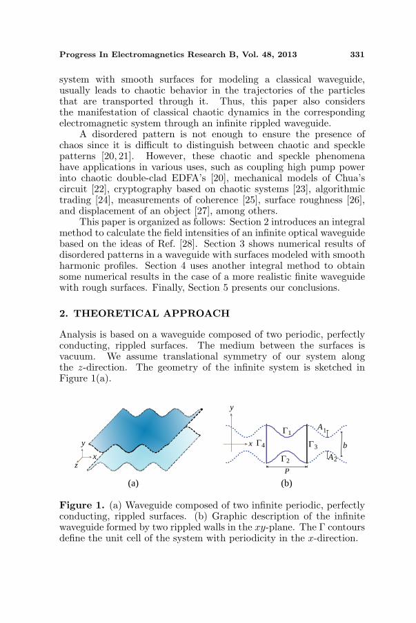
Analysis is based on a waveguide composed of two periodic, perfectlyconducting, rippled surfaces. The medium between the surfaces isvacuum. We assume translational symmetry of our system alongthe z-direction. The geometry of the infinite system is sketched inFigure 1(a).

y

x

P

b 4

1

2

3

A 1

A 2

y

x z

Γ

Γ

Γ Γ

(a) (b)

Figure 1. (a) Waveguide composed of two infinite periodic, perfectlyconducting, rippled surfaces. (b) Graphic description of the infinitewaveguide formed by two rippled walls in the xy-plane. The Γ contoursdefine the unit cell of the system with periodicity in the x-direction.


In order to describe the infinite waveguide formed by two rippledwalls in the xy-plane (shown in Figure 1(b)), we consider that theperiodic profiles of the walls have period P , that the average widthof the waveguide is given by b, and that the surface profiles can berepresented by the harmonic functions b/2 + A1 cos(2πx/P ) (upperprofile) and −b/2 + A2 cos(2πx/P − ∆φ) (lower profile), where A1

and A2 represent the amplitudes and ∆φ stands for a phase differencebetween the two profiles. The region enclosed by the curves Γ1, Γ2,Γ3 and Γ4 can be considered as a unit cell of the system. The setof an infinite number of unit cells is a waveguide of infinite lengthrepresented by a perfect crystal. A finite number (large enough) ofunit cells is a waveguide of finite length represented by a truncatedcrystal (see Ref. [13]).

Let us consider the problem of finding the electromagnetic fieldinside the waveguide. An integral method is used that can beformulated by following the same ideas developed elsewhere [28–30].This problem can be studied using the scalar theory by considering twocomplementary polarization states given the symmetry of our physicalsystem along the z-direction. This work considers only the case of anelectromagnetic field with TE polarization with Ez representing thez-component of the electric field.

It is well-known that the function Ez(r) satisfies the Helmholtzequation

∇2Ez (r) +(ω

c

)2Ez (r) = 0, (1)

where ω is the frequency of the electromagnetic wave, c the speed oflight in vacuum, and r =xı + y a two-dimensional vector independentof the coordinate z.

The periodicity in the x-direction is another symmetry conditionthat is considered. Due to this property and the form of the differentialequation Eq. (1), the Bloch theorem can be applied for the x-direction.In this way, the following expression can be derived

Ez (x− P, y) = exp (−ikP ) Ez (x, y) , (2)

where k is the one-dimensional Bloch vector.In order to determine the electric field, first of all we have to find

the dispersion relation ω = ω(k). With this in mind, let us considera Green’s function for a two-dimensional geometry that can be usedto solve the Helmholtz equation. The Green’s function considered isG(r, r′) = iπH

(1)0 (K|r − r′|), where H

(1)0 (%) is the Hankel function of

the first kind and zero order, and K = ω/c. Considering the geometryof the unit cell shown in Figure 1(b) and applying the two-dimensionalsecond Green’s theorem for the functions Ez and G, we obtain the


expression14π

∮

Γ

[G(r, r′)

∂Ez(r′)∂n′

− ∂G(r, r′)∂n′

Ez(r′)]

ds′ = Ez (r) θ (r) , (3)

being θ(r) = 1 if r is inside the unit cell and θ(r) = 0 otherwise. ds′ isthe differential arc’s length, n′ the outward normal vector to Γ, and theobservation point r is infinitesimally separated of contour Γ outer to theunit cell. The geometry of the problem is described by representing thepoints along the contour Γ with Cartesian coordinates X(s′), Y (s′) asparametric functions of the arc’s length s′ and their derivatives X ′(s′),Y ′(s′), X ′′(s′) and Y ′′(s′), up to second order.

In order to solve numerically Eq. (3), we divide the curve Γ infour segments Γ1, Γ2, Γ3 and Γ4 (Fig. 1(b)) and take a samplingXn = X(sn), Yn = Y (sn) along the each curve. The correspondingnumber of points along the curves are N1, N2, N3 and N4 respectively,and N = N1 + N2 + N3 + N4 to the total number of points isdefined. It is important to mention that the points (Xn, Yn) onΓ3 must be corresponding to those on Γ4 (Xn − P, Yn), in this wayN3 = N4. Besides these considerations, we take into account theboundary condition at the perfectly conducting surfaces (with curvesΓ1 and Γ2). Therefore, Eq. (3) can be represented numerically in termsof a homogeneous system of N algebraic equations as follows:

N1∑

n=1

Lmn(1)Φn(1) +N2∑

n=1

Lmn(2)Φn(2) +N3∑

n=1

Lmn(3)Φn(3)

−N3∑

n=1

Nmn(3)Ψn(3) +N4∑

n=1

Lmn(4)Φn(4) −N4∑

n=1

Nmn(4)Ψn(4) = 0, (4)

for m = 1, 2, . . . , N . In Eq. (4) the source functions Ψn(3) and Φn(j)represent numerically the field Ez and its normal derivative. Besides,the subscripts n(j), j = 1, 2, 3, 4 denote the n-th point along the Γj

contour. The matrix element Lmn(j) and Nmn(j) are given by [28, 29]

Lmn(j) = i∆s

4H

(1)0

(ω

cdmn

)(1− δmn) + i

∆s

4H

(1)0

(ω

c

∆s

2e

)δmn , (5)

and

Nmn(j) = i∆s

4ω

cH

(1)1

(ω

cdmn

) Dmn

dmn(1−δmn)+

(12+

∆s

4πD′

n

)δmn , (6)

where

dmn =√

(Xm −Xn)2 + (Ym − Yn)2, (7)

Dmn = −Y ′n (Xm −Xn) + X ′

n (Ym − Yn) , (8)


D′n = X ′

nY ′′n −X ′′

nY ′n. (9)

H(1)1 (%) is the Hankel’s function of first kind and first order. The

function δ(j)mn represents the Kronecker’s delta and ∆s is the arc’s length

between two consecutive points of a given curve. In Eqs. (8) and (9),we have defined X ′

n = X ′(s)|s=sn , X ′′n = X ′′(s)|s=sn , and so forth.

For simplicity we have omitted the contour index (j) but it must beimplicitly understood that n = n(j) wherever it appears in Eqs. (5)–(9).

By applying Eq. (2) we obtain the equations Ψ(4)n =

exp(−ikP )Ψ(3)n , and Φ(4)

n = − exp(−ikP )Φ(3)n . The minus sign

appearing in last equation results because the normals to correspondingpoints at Γ3 and Γ4 have opposite directions. Using these equations,we obtain

N1∑

n=1

Lmn(1)Φn(1)+N2∑

n=1

Lmn(2)Φn(2)+N3∑

n=1

(Lmn(3)−exp (−ikP ) Lmn(4)

)

×Φn(3) −N3∑

n=1

(Nmn(3) + exp (−ikP ) Nmn(4)

)Ψn(3) = 0, (10)

with m = 1, 2, . . . , N . Eq. (10) constitutes a linear system that has anassociated representative matrix, Mmn , that depends on the frequencyω and the Bloch vector k. Since the equation system is homogeneous,a nontrivial solution can be obtained if the determinant of such matrixdefined as

D (k, ω) = ln (|det (M)|) (11)

is zero. Numerically this function (Eq. (11)) presents local minimumpoints that will give us the numeric dispersion relation ω = ω(k).

For our purposes, this work requires analyzing the intensity,defined by E∗

zEz, in a unit cell. In order to calculate it for a eigenmodeat a given point (k, ω), one must consider the dispersion relationobtained numerically by the use of a homogeneous equation system.Additional details of the numerical method employed can be found inRef. [13].

3. CLASSICAL CHAOTIC BEHAVIOR AND ITSELECTROMAGNETIC COUNTERPART

We mentioned above that the geometry of the proposed system hereinhas been considered in order to study its quantum and classicaltransport properties [12, 18, 19]. According to this study, the system


analyzed could present some signatures of electromagnetic wave chaosfor certain parameters.

We shall calculate certain eigenmodes in the unit cell to observesome traces of the chaotic behavior of our system. But first thecorresponding classical system must be examined to demonstrate thepresence of chaos.

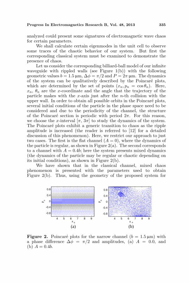
Let us consider the corresponding billiard-ball model of our infinitewaveguide with rippled walls (see Figure 1(b)) with the followinggeometric values b = 1.5µm, ∆φ = π/2 and P = 2π µm. The dynamicsof the system can be qualitatively described by the Poincare plots,which are determined by the set of points (xn, pn = cos θn). Here,xn, θn are the x-coordinate and the angle that the trajectory of theparticle makes with the x-axis just after the n-th collision with theupper wall. In order to obtain all possible orbits in the Poincare plots,several initial conditions of the particle in the phase space need to beconsidered and due to the periodicity of the channel, the structureof the Poincare section is periodic with period 2π. For this reason,we choose the x-interval [π, 3π] to study the dynamics of the system.The Poincare plots exhibit a generic transition to chaos as the rippleamplitude is increased (the reader is referred to [12] for a detaileddiscussion of this phenomenon). Here, we restrict our approach to justtwo cases. The first is the flat channel (A = 0), where the dynamics ofthe particle is regular, as shown in Figure 2(a). The second correspondsto a channel with A = 0.4b; here the system presents mixed dynamics(the dynamics of the particle may be regular or chaotic depending onits initial conditions), as shown in Figure 2(b).

We have shown that in the classical channel, mixed chaosphenomenon is presented with the parameters used to obtainFigure 2(b). Thus, using the geometry of the proposed system for

pn

pn

-0.8

-0.4

0

0.4

0.8

-0.8

-0.4

0

0.4

0.8

4 5 6 7 8 9x n

4 5 6 7 8 9x n

(a) (b)

Figure 2. Poincare plots for the narrow channel (b = 1.5µm) witha phase difference ∆φ = π/2 and amplitudes, (a) A = 0.0, and(b) A = 0.4b.


x [µm]0 2 4 6

1

2

3

4

5

6

x 10 -4

0 2 4 6 8x [µm]

x [µm]0 2 4 6

0.511.522.533.54

x 10 -8

0 2 4 6 8x [µm]

(a) (b)

(c) (d)

y [µ

m]

-0.5

0

0.5

1

1.5

2

-1

-0.5

0

0.5

1

Aut

ocor

rela

tion

Fun

ctio

n

-1

-0.5

0

0.5

1

Aut

ocor

rela

tion

Fun

ctio

n

y [µ

m]

-0.5

0

0.5

1

1.5

2

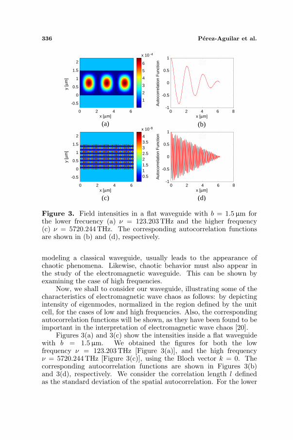
Figure 3. Field intensities in a flat waveguide with b = 1.5µm forthe lower frecuency (a) ν = 123.203THz and the higher frequency(c) ν = 5720.244THz. The corresponding autocorrelation functionsare shown in (b) and (d), respectively.

modeling a classical waveguide, usually leads to the appearance ofchaotic phenomena. Likewise, chaotic behavior must also appear inthe study of the electromagnetic waveguide. This can be shown byexamining the case of high frequencies.

Now, we shall to consider our waveguide, illustrating some of thecharacteristics of electromagnetic wave chaos as follows: by depictingintensity of eigenmodes, normalized in the region defined by the unitcell, for the cases of low and high frequencies. Also, the correspondingautocorrelation functions will be shown, as they have been found to beimportant in the interpretation of electromagnetic wave chaos [20].

Figures 3(a) and 3(c) show the intensities inside a flat waveguidewith b = 1.5µm. We obtained the figures for both the lowfrequency ν = 123.203 THz [Figure 3(a)], and the high frequencyν = 5720.244THz [Figure 3(c)], using the Bloch vector k = 0. Thecorresponding autocorrelation functions are shown in Figures 3(b)and 3(d), respectively. We consider the correlation length l definedas the standard deviation of the spatial autocorrelation. For the lower


frequency, the correlation length was l = 0.4133, while for the higherfrequency it was l = 0.4123. In the case of a waveguide with flat walls,no chaos phenomenon appears. This is a straightforward statement andone easily to understand. As a result, similar values for the correlationlengths were obtained.

In order to make reliable calculations in the case of highfrequencies, it is necessary to use small discretization intervals. Dueto numerical approximations involved, ∆s = c/20νmax ≈ 0.0026µmwas used. This value produced a good resolution in our calculations,which was then verified by comparing the numerical results with thecorresponding analytical results for the flat waveguide.

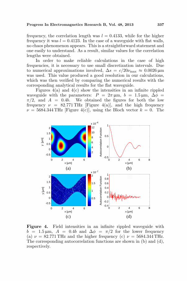
Figures 4(a) and 4(c) show the intensities in an infinite rippledwaveguide with the parameters: P = 2π µm, b = 1.5µm, ∆φ =π/2, and A = 0.4b. We obtained the figures for both the lowfrequency ν = 82.771THz [Figure 4(a)], and the high frequencyν = 5684.344THz [Figure 4(c)], using the Bloch vector k = 0. The

x [µm]

y [µ

m]

0 2 4 6

-0.5

0

0.5

1

1.5

2

2

4

6

8

10

12x 10 -4

0 2 4 6 8-0.5

0

0.5

1

x [µm]

Aut

ocor

rela

tion

Fun

ctio

n

x [µm]

y [µ

m]

0 2 4 6

-0.5

0

0.5

1

1.5

2

0.5

1

1.5

2x 10 -7

0 2 4 6 8x [µm]

Aut

ocor

rela

tion

Fun

ctio

n

(a) (b)

(c) (d)

-0.4

-0.2

0

0.2

0.4

0.6

0.8

1

Figure 4. Field intensities in an infinite rippled waveguide withb = 1.5µm, A = 0.4b and ∆φ = π/2 for the lower frequency(a) ν = 82.771THz and the higher frequency (c) ν = 5684.344THz.The corresponding autocorrelation functions are shown in (b) and (d),respectively.


corresponding autocorrelation functions are shown in Figures 4(b)and 4(d), respectively. For the lower frequency, the correlation lengthwas l = 0.3241, while for the higher frequency it was l = 0.0977.

Upon comparing the correlation lengths obtained, the latter casehad a small value for the parameter l. We believe this is a manifestationof electromagnetic wave chaos, since in this regime led us to thinkthat the intensity of the eigenmode is an uncorrelated random variableas a function of a point (x, y) in the unit cell. In this case, theintensity cannot be represented by a function with smooth variationsthat give rise to the appearance of disordered peaks. This effect isalso a characteristic of quantum chaos (see Ref. [18]). A disorderedpattern is not enough to ensure the presence of chaos; nevertheless,the corresponding classical channel obviously presents chaos behavior,and this is our main argument.

4. FINITE ROUGH WAVEGUIDE

In the previous section, Figure 4(c) was included to show somesignatures of chaotic behavior using the intensity of the eigenmodein the real space. Other results are shown in a similar way inRef. [20, 21]. It is well known that the surfaces of materials alwayshave a certain degree of roughness, and that is difficult to distinguishchaotic patterns from speckle patterns [20]. This motivated us topresent some calculations for waveguides with rough surfaces that giverise to intensities with disordered patterns; patterns that are similar tothose shown in Figure 4(c). This makes it possible to present a systemin which chaos and speckle appear simultaneously.

25

20

15

10

5

00.5

1

1.5

2

2.5

3

3.5

4

0

1

2

3

4

5

6

(a) (b)

0 1 2Scattered angle [rad]

-1 -20 5 10 15 20 25 30 35x [µm]

-5-10

Ref

lect

ed In

tens

ity

z [ µ

m]

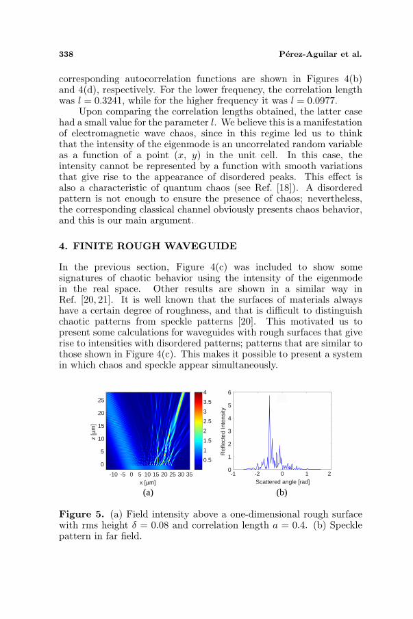
Figure 5. (a) Field intensity above a one-dimensional rough surfacewith rms height δ = 0.08 and correlation length a = 0.4. (b) Specklepattern in far field.


The speckle effect occurs if the size of surface roughness is aroundof the wavelength of the incident beam [31]. With this in mind, onecan properly choose the parameters for the numerical simulations. Asan example, Figure 5(a) shows the speckle pattern (field intensity)by a one-dimensional perfectly conducting rough surface. The surfaceis illuminated at 30 degrees by a Gaussian beam with a wavelengthλ = 0.6120µm. The roughness profile is a certain realization of anensemble used to model a random surface with Gaussian statistics.The ensemble has a mean profile that corresponds to a flat surface.The theoretical parameters assumed in obtaining these results werethe length correlation a = 0.4µm and the rms height δ = 0.08 µmfor the frequency ν = 490.1940THz [32]. The corresponding specklepattern in far field zone is shown in Figure 5(b).

As a consequence of the surface roughness on the scale of theoptical wavelength, the various wavefronts are added with markedlydifferent phases, resulting in a highly complex pattern of interference.The image of this pattern [Figure 5(a)] is found to have threads (orgranular) appearance with a multitude of bright and dark threads (orspots). This calculation also makes it possible to see the scatteredfield intensity in the far field zone, which appears as a curve with veryabrupt changes [Figure 5(b)].

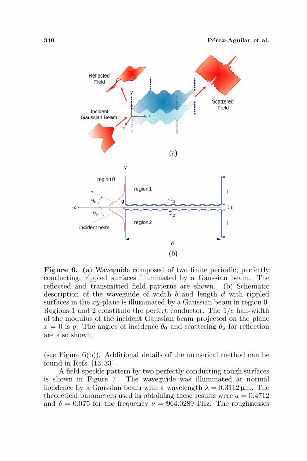
Now, another of our interests was to obtain speckle patterns in awaveguide formed by rough surfaces. For this case, it is necessaryto consider a finite waveguide composed of two periodic, perfectlyconducting, rippled surfaces illuminated by an incident electromagneticwave, as shown in Figure 6(a). To approach this problem, someconsiderations must be assumed and we shall bear in mind it in thexy-plane. Since the size of the system is finite, to avoid edge effectswe illuminate it with a tapered Gaussian beam whose intercept withthe plane of the channel has a half-width g. This parameter must besmaller than the total length of the system Ly = 2l + b, but muchlarger than the width of the aperture b (see Figure 6(b)).

Under these considerations, the incident field can be expressed interms of its angular spectrum A(q, k‖)

Ψinc(x, y) =

ω/c∫

−ω/c

dq

2πA(q, k‖) exp{i [qx− α0(q)y]}, (12)

where α0(q) = [(ω/c)2 − q2]1/2 with <e α0(q) > 0 and =mα0(q) > 0.In this work we choose

A(q, k‖) =√

πg exp{−g2(q − k‖)2/4

}, (13)

where the parameter k‖ = (ω/c) sin θ0, being θ0 the angle of incidence


y

x

z

Incident Gaussian Beam

Scattered Field

Reflected Field

region 1

b

d

C 2

C 1

region 2

0

s

y

region 0

incident bea m l

l

g -x

(a)

(b)

θ

θ

Figure 6. (a) Waveguide composed of two finite periodic, perfectlyconducting, rippled surfaces illuminated by a Gaussian beam. Thereflected and transmitted field patterns are shown. (b) Schematicdescription of the waveguide of width b and length d with rippledsurfaces in the xy-plane is illuminated by a Gaussian beam in region 0.Regions 1 and 2 constitute the perfect conductor. The 1/e half-widthof the modulus of the incident Gaussian beam projected on the planex = 0 is g. The angles of incidence θ0 and scattering θs for reflectionare also shown.

(see Figure 6(b)). Additional details of the numerical method can befound in Refs. [13, 33].

A field speckle pattern by two perfectly conducting rough surfacesis shown in Figure 7. The waveguide was illuminated at normalincidence by a Gaussian beam with a wavelength λ = 0.3112µm. Thetheoretical parameters used in obtaining these results were a = 0.4712and δ = 0.075 for the frequency ν = 964.0289 THz. The roughnesses


x [µm]

0 5 10 15 20

y [µ

m]

-0.5

0

0.5

1

1.5

2

-1.5

-1

-21234567891011

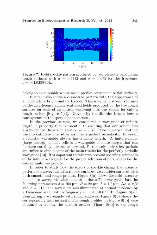
Figure 7. Field speckle pattern produced by two perfectly conductingrough surfaces with a = 0.4712 and δ = 0.075 for the frequencyν = 964.0289THz.

belong to an ensemble whose mean profiles correspond to flat surfaces.Figure 7 also shows a disordered pattern with the appearance of

a multitude of bright and dark spots. This irregular pattern is formedby the interference among scattered fields produced by the two roughsurfaces on scale of an optical wavelength, as was shown for only arough surface [Figure 5(a)]. Obviously, the disorder is seen here aconsequence of the speckle phenomenon.

In the previous section, we considered a waveguide of infinitelength, a property that is essential to ensuring that our system hasa well-defined dispersion relation ω = ω(k). The numerical methodused to calculate intensities assumes a perfect periodicity. However,a realistic waveguide always has a finite length. A finite number(large enough) of unit cells is a waveguide of finite length that canbe represented by a truncated crystal. Fortunately, only a few periodsare suffice to obtain some of the main results for the perfectly periodicwaveguide [13]. It is important to take into account specific eigenmodesof the infinite waveguide for the proper selection of parameters for thecase of finite waveguides.

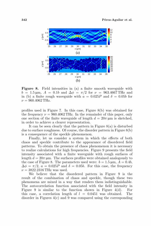
In order to study how the effects of speckle change the intensitypattern of a waveguide with rippled surfaces, we consider surfaces withboth smooth and rough profiles. Figure 8(a) shows the field intensityin a finite waveguide with smooth surfaces.The waveguide has thefollowing parameters d = 20π µm, P = 2π µm, b = 1.5µm, ∆φ = π/2and A = 0.1b. The waveguide was illuminated at normal incidence bya Gaussian beam with a frequency ν = 963.4667THz [Figure 8(a)].Considering a waveguide with rough surfaces, Figure 8(b) shows thecorresponding field intensity. The rough profiles [in Figure 8(b)] wereobtained by adding the smooth profiles [Figure 8(a)] to the rough


x [µm]

y [µ

m]

25 26 27 28 29 30 31 32 33 34 35

24681012

25 26 27 28 29 30 31 32 33 34 35

1020304050607080

(a)

y [µ

m]

x [µm]

(b)

0

0.5

1

-0.5

-1

0

0.5

1

-0.5

-1

Figure 8. Field intensities in (a) a finite smooth waveguide withb = 1.5µm, A = 0.1b and ∆φ = π/2 for ν = 963.4667THz andin (b) a finite rough waveguide with a = 0.025P and δ = 0.05b forν = 960.4062THz.

profiles used in Figure 7. In this case, Figure 8(b) was obtained forthe frequency ν = 960.4062THz. In the remainder of this paper, onlyone section of the finite waveguide of length d = 20π µm is sketched,in order to achieve a clearer representation.

It can be seen clearly that the pattern in Figure 8(a) is disturbeddue to surface roughness. Of course, the disorder pattern in Figure 8(b)is a consequence of the speckle phenomenon.

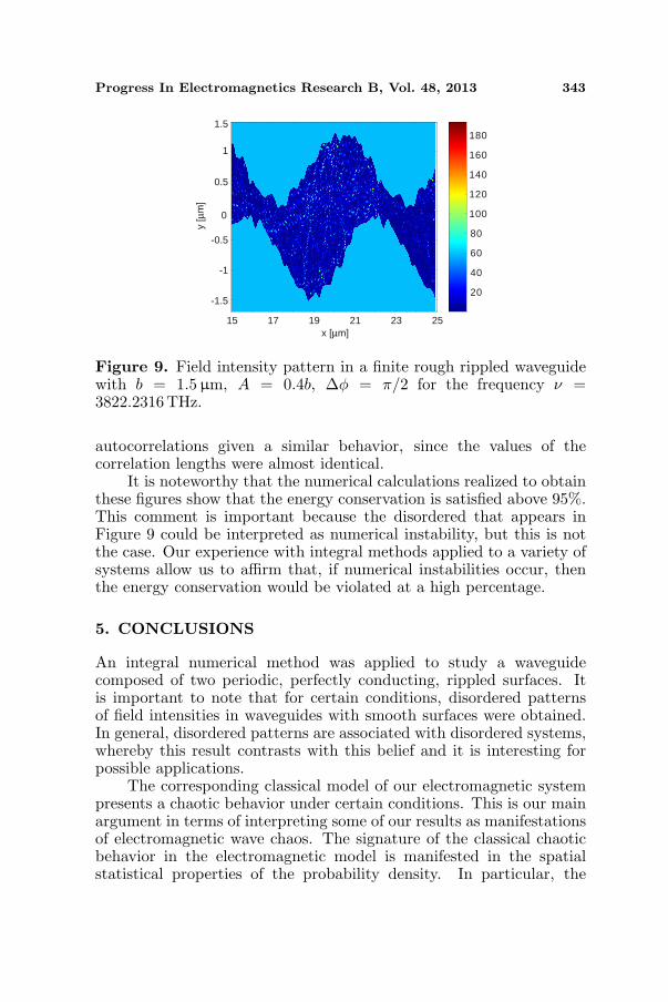
Finally, let us consider a system in which the effects of bothchaos and speckle contribute to the appearance of disordered fieldpatterns. To obtain the presence of chaos phenomenon it is necessaryto realize calculations for high frequencies. Figure 9 presents the fieldintensity associated with a finite waveguide with rough surfaces oflength d = 20π µm. The surfaces profiles were obtained analogously tothe case of Figure 8. The parameters used were: b = 1.5µm, A = 0.4b,∆φ = π/2, a = 0.025P and δ = 0.05b. For this case, the frequencyν = 3822.2316THz was used.

We believe that the disordered pattern in Figure 9 is theresult of the combination of chaos and speckle, though these twophenomena are mixed in a way that renders them indistinguishable.The autocorrelation function associated with the field intensity inFigure 9 is similar to the function shown in Figure 4(d). Forthis case, a correlation length of l = 0.0451 was obtained. Thedisorder in Figures 4(c) and 9 was compared using the corresponding


15 17 19 21 23 25

20

40

60

80

100

120

140

160

180

x [µm]

y [µ

m]

-0.5

0.5

1.5

-1.5

-1

0

1

Figure 9. Field intensity pattern in a finite rough rippled waveguidewith b = 1.5µm, A = 0.4b, ∆φ = π/2 for the frequency ν =3822.2316THz.

autocorrelations given a similar behavior, since the values of thecorrelation lengths were almost identical.

It is noteworthy that the numerical calculations realized to obtainthese figures show that the energy conservation is satisfied above 95%.This comment is important because the disordered that appears inFigure 9 could be interpreted as numerical instability, but this is notthe case. Our experience with integral methods applied to a variety ofsystems allow us to affirm that, if numerical instabilities occur, thenthe energy conservation would be violated at a high percentage.

5. CONCLUSIONS

An integral numerical method was applied to study a waveguidecomposed of two periodic, perfectly conducting, rippled surfaces. Itis important to note that for certain conditions, disordered patternsof field intensities in waveguides with smooth surfaces were obtained.In general, disordered patterns are associated with disordered systems,whereby this result contrasts with this belief and it is interesting forpossible applications.

The corresponding classical model of our electromagnetic systempresents a chaotic behavior under certain conditions. This is our mainargument in terms of interpreting some of our results as manifestationsof electromagnetic wave chaos. The signature of the classical chaoticbehavior in the electromagnetic model is manifested in the spatialstatistical properties of the probability density. In particular, the


correlation length of the autocorrelation function goes to zero whenthe corresponding classical system is chaotic.

It is also possible to obtain a disordered pattern for low frequenciesby the effect of roughness that produces a speckle pattern. This allowsus to extend the frequency range for obtaining disordered patterns.

Since the surfaces of materials always have a certain degree ofroughness, it can be concluded that both chaos and speckle contributeto the presence of disordered field patterns.

ACKNOWLEDGMENT

The authors wish to express their gratitude to Consejo Nacional deCiencia y Tecnologıa (Mexico) for financial support through grant54770, to the Coordinacion de la Investigacion Cientıfica at theUniversidad Michoacana de San Nicolas de Hidalgo, and to the Red deCuerpos Academicos PROMEP-SEP (FOFM-2008).

REFERENCES

1. Shen, J.-T. and S. Fan, “Strongly correlated two-electrontransport in a quantum waveguide having a single Andersonimpurity,” New J. Phys., No. 11, 113024, 2009.

2. Rayleigh, L., “On the resultant of a large number of vibrationsof the same pitch and of arbitrary phase,” Phil. Mag., Vol. 10,73–78, 1880.

3. Rigden, J. D. and E. I. Gordon, “The granularity of scatteredoptical maser light,” Proc. IRE, Vol. 50, 2367–2368, 1962.

4. Oliver, B. M., “Sparkling spots and random diffraction,” Proc.IEEE, Vol. 5, 220–221, 1963.

5. Sheng, P., Scattering and Localization of Classical Waves inRandom Media, World Scientific Publishing, Singapore, 1990.

6. Anderson, P. W., “Absence of diffusion in certain randomlattices,” Phys. Rev. B, Vol. 109, No. 5, 1492–1505, 1958.

7. Michel, T. R. and K. A. O’Donnell, “Angular correlation functionsof amplitudes scattered from a one-dimensional, perfectlyconducting rough surface,” J. Opt. Soc. Am. A, Vol. 9, No. 8,1374–1384, 1992.

8. Webb, R. A., S. Washburn, C. P. Umbach, and R. B. Laibowitz,“Observation of h/e Aharonov-Bohm oscillations in normal-metalrings,” Phys. Rev. Lett., Vol. 54, No. 25, 2696–2699, 1985.

9. Mirlin, A. D., A. Muller-Groeling, and M. R. Zirnbauer,


“Conductance fluctuations of disordered wires: Fourier analysison supersymmetric spaces,” Ann. Phys., Vol. 236, 325–373, 1994.

10. Chang, A. M., H. U. Baranger, L. N. Pfeiffer, and K. W. West,“Weak localization in chaotic versus nonchaotic cavities: Astriking difference in the line shape,” Phys. Rev. Lett., Vol. 73,No. 15, 2111–2114, 1994.

11. Luna-Acosta, G. A., A. A. Krokhin, M. A. Rodrıguez, andP. H. Hernandez-Tejeda, “Classical chaos and ballistic transportin a mesoscopic channel,” Phys. Rev. B, Vol. 54, No. 16, 11410–11416, 1996.

12. Herrera-Gonzalez, I. F., G. Arroyo-Correa, A. Mendoza-Suarez,and E. S. Tututi, “Study of the resistivity in a channel withdephased ripples,” Int. J. Mod. Phys. B, Vol. 25, 683–698, 2011.

13. Mendoza-Suarez, A., H. Perez-Aguilar, and F. Villa-Villa,“Optical response of a perfect conductor waveguide that behavesas a photonic crystal,” Progress In Electromagnetics Research,Vol. 121, 433–452, 2011.

14. Zhang, G. G., H. Zhang, Z. L. Yuan, Z. M. Wang, and D. Wang,“A novel broadband E-plane omni-directional planar antenna,”Journal of Electromagnetic Waves and Applications, Vol. 24,Nos. 5–6, 663–670, 2010.

15. Ye, H., H. Wang, S. P. Yeo, and C. Qiu, “Finite-boundarybowtie aperture antenna for trapping nanoparticles,” Progress InElectromagnetics Research, Vol. 136, 17–27, 2013.

16. Sanchez-Escuderos, D., M. Ferrando-Bataller, J. I. Herranz,and M. Baquero-Escudero, “Optimization of the E-plane loadedrectangular waveguide for low-loss propagation,” Progress InElectromagnetics Research, Vol. 135, 411–433, 2013.

17. Inoue, K. and K. Ohkata, Photonic Crystals, Springer, Germany,2004.

18. Luna-Acosta, G. A., K. Na, L. E. Reichl, and A. Krokhin, “Bandstructure and quantum Poincare sections of a classically chaoticquantum rippled channel,” Phys. Rev. E, Vol. 53, No. 4, 3271–3283, 1996.

19. Herrera-Gonzalez, I. F., H. I. Perez-Aguilar, A. Mendoza-Suarez,and E. S. Tututi, “Heat conduction in systems with Kolmogorov-Arnold-Moser phase space structure,” Phys. Rev. E, Vol. 86, No. 3,031138-1–031138-9, 2012.

20. Doya, V., O. Legrand, and F. Mortessagne, “Light scarring in anoptical fiber,” Phys. Rev. Lett., Vol. 88, No. 1, 014102–014105,2002.


21. Wilkinson, P. B., T. M. Fromhold, R. P. Taylor, andA. P. Micolich, “Electromagnetic wave chaos in gradient refractiveindex optical cavities,” Phys. Rev. Lett., Vol. 86, No. 24, 5466–5469, 2001.

22. Awrejcewicz, J. and M. L. Calvisi, “Mechanical models of Chua’scircuit,” Int. J. Bif. and Chaos, Vol. 12, No. 4, 671–686, 2002.

23. Yang, T., C. W. Wu, and L. O. Chua, “Impulsive stabilizationfor control and synchronization of chaotic systems: Theory andapplication to secure communication,” IEEE Trans. Circuits Syst.— I, Vol. 44, No. 10, 976–988, 1997.

24. Williams, B. and J. Williams, Trading chaos: Maximize Profitswith Proven Technical Techniques, Wiley, New York, 2004.

25. Asakura, T., H. Fuji, and K. Murata, “Measurement of spatialcoherence using speckle patterns,” Opt. Acta, Vol. 19, 273, 1972.

26. Crane, R. B., “Use of a laser-produced speckle pattern todetermine surface roughness,” J. Opt. Soc. Am., Vol. 60, No. 12,1658–1663, 1970.

27. Tiziani, H. J., “Analysis of mechanical oscillations by speckling,”Appl. Opt., Vol. 11, No. 12, 2911–2917, 1972.

28. Mendoza-Suarez, A., F. Villa-Villa, and J. A. Gaspar-Armenta,“Numerical method based on the solution of integral equations forthe calculation of the band structure and reflectance of one- andtwo-dimensional photonic crystals,” J. Opt. Soc. Am. B, Vol. 23,No. 10, 2249–2256, 2006.

29. Mendoza-Suarez, A., F. Villa-Villa, and J. A. Gaspar-Armenta,“Band structure of two-dimensional photonic crystals that includedispersive left-handed materials and dielectrics in the unit cell,”J. Opt. Soc. Am. B, Vol. 24, No. 12, 3091–3098, 2007.

30. Villa-Villa, F., J. A. Gaspar-Armenta, and A. Mendoza-Suarez,“Surface modes in one dimensional photonic crystals that includeleft handed materials,” Journal of Electromagnetic Waves andApplications, Vol. 21, No. 4, 485–499, 2007.

31. Goodman, J. W., Speckle Phenomena in Optics: Theory andApplications, Roberts & Co., USA, 2007.

32. Leskova, T. A., A. A. Maradudin, “Multiple-scattering effectsin angular intensity correlation functions,” Light Scattering andNanoscale Surface Roughness, A. A. Maradudin (ed.), Springer-Verlag, New York, 2007.

33. Perez, H. I., E. R. Mendez, C. I. Valencia, and J. A. Sanchez-Gil,“On the transmission of diffuse light through thick slits,” J. Opt.Soc. Am. A, Vol. 26, No. 4, 909–918, 2009.

DISORDERED FIELD PATTERNS IN A WAVEGUIDE WITH PERIODIC ...

Documents

Transcript of DISORDERED FIELD PATTERNS IN A WAVEGUIDE WITH PERIODIC ...