Disentangling Credit Spreads and Equity Volatility · Pierre-Olivier Weill, and participants in...
90
Disentangling Credit Spreads and Equity Volatility * CLICK HERE FOR LATEST VERSION Adrien d’Avernas † January 31, 2017 Abstract In this paper, I provide a structural approach to quantify the forces that govern the joint dynamics of corporate bond credit spreads and equity volatility. I build a dynamic model and estimate a wide array of funda- mental shocks using a large firm-level database on credit spreads, equity prices, accounting statements, and bond recovery ratios in the U.S. from 1973 to 2014. A structural decomposition reveals that the joint dynam- ics of credit spreads and equity volatility is driven by fluctuations in firms’ asset values and aggregate asset volatility. I find that aggregate asset volatility captures the informational content of credit spreads for predicting economic activity. All together, my results suggest that ag- gregate asset volatility is key for the transmission channel that links the fundamental drivers of financial indicators to the real economy. * I am deeply indebted to Andrew Atkeson and Lee Ohanian for their dedicated supervision, unlimited availability, and infinite patience. I also would like to thank, for fruitful discussions and comments, Saki Bigio, Andrea Eisfeldt, Fran¸cois Geerolf, Semih ¨ Usl¨ u, Quentin Vandeweyer, Pierre-Olivier Weill, and participants in seminars at UCLA Economics and Anderson Finance, the Minnesota Federal Reserve Bank, the Richmond Federal Reserve Bank, the San Francisco Federal Reserve Bank, and the Becker Friedman Institute. † UCLA 1
Transcript of Disentangling Credit Spreads and Equity Volatility · Pierre-Olivier Weill, and participants in...
Disentangling Credit Spreads and Equity Volatility∗
CLICK HERE FOR LATEST VERSION
Adrien d’Avernas†
January 31, 2017
Abstract
In this paper, I provide a structural approach to quantify the forces that
govern the joint dynamics of corporate bond credit spreads and equity
volatility. I build a dynamic model and estimate a wide array of funda-
mental shocks using a large firm-level database on credit spreads, equity
prices, accounting statements, and bond recovery ratios in the U.S. from
1973 to 2014. A structural decomposition reveals that the joint dynam-
ics of credit spreads and equity volatility is driven by fluctuations in
firms’ asset values and aggregate asset volatility. I find that aggregate
asset volatility captures the informational content of credit spreads for
predicting economic activity. All together, my results suggest that ag-
gregate asset volatility is key for the transmission channel that links the
fundamental drivers of financial indicators to the real economy.
∗I am deeply indebted to Andrew Atkeson and Lee Ohanian for their dedicated supervision,unlimited availability, and infinite patience. I also would like to thank, for fruitful discussionsand comments, Saki Bigio, Andrea Eisfeldt, Francois Geerolf, Semih Uslu, Quentin Vandeweyer,Pierre-Olivier Weill, and participants in seminars at UCLA Economics and Anderson Finance, theMinnesota Federal Reserve Bank, the Richmond Federal Reserve Bank, the San Francisco FederalReserve Bank, and the Becker Friedman Institute.†UCLA
1
1 Introduction
Indicators of financial distress and uncertainty, such as corporate bond credit spreads
and equity volatility, are powerful predictors of real economic activity.1 Understand-
ing what are the fundamental drivers of these financial indicators is critical to com-
prehend the linkages between financial markets and the real economy.
Yet, it remains difficult to assess empirically which shocks are important in ac-
counting for the dynamics of these financial indicators. The high degree of comove-
ment complicates the identification of fundamental shocks (see Stock and Watson,
2012, and Caldara, Fuentes-Albero, Gilchrist, and Zakrajsek, 2016). To address this
challenge, I propose a dynamic structural model with shocks to firms’ asset values,
bankruptcy costs, firms’ aggregate and idiosyncratic asset volatility, and the market
price of risk. I structurally estimate the shocks with a large firm-level database on
credit spreads, equity prices, accounting statements, and bond recovery ratios in the
U.S. from 1973 to 2014. The model accurately accounts for the historical levels and
dynamics, both over time and in the cross-section, of five financial indicators: (i)
default risk, (ii) corporate bond credit spreads, (iii) aggregate and (iv) idiosyncratic
equity volatility, and (v) corporate bond bid-ask spreads. A structural decomposi-
tion yields that shocks to firms’ asset values and aggregate asset volatility are key to
account for the joint dynamics of these financial indicators. Moreover, fluctuations
in firms’ aggregate asset volatility strongly predict future economic activity.
My structural model primarily builds on Chen, Cui, He, and Milbradt (2016).
There are two types of shocks in this economy: small and frequent shocks to firms’
asset values and large but infrequent shocks to macroeconomic conditions. Fluc-
tuations in macroeconomic conditions include shocks to bankruptcy costs, firms’
aggregate and idiosyncratic asset volatility, and the market price of risk. Firms’
assets generate cash flows and are financed through equity and debt. Firms’ asset,
equity, and debt are priced by a common stochastic discount factor. The optimal
capital structure of firms is based on the trade-off between tax benefits of debt and
1See Philippon (2009); Bloom (2009); Stock and Watson (2012); Gilchrist and Zakrajsek(2012), Caldara, Fuentes-Albero, Gilchrist, and Zakrajsek (2016); Herskovic, Kelly, Lustig, andVan Nieuwerburgh (2016); and many others.
2

deadweight losses of default. Firms decide when to default based on their cash flow
level and macroeconomic conditions. The secondary market for corporate bonds is
subject to over-the-counter liquidity frictions.
In the model, over-the-counter market illiquidity—and consequently bid-ask
spreads—arise endogenously as in Chen, Cui, He, and Milbradt (2016). Investors
face uninsurable idiosyncratic liquidity shocks, which drive up their costs of holding
corporate bonds. To sell their bonds, investors must search for dealers to intermedi-
ate transactions with other investors. In the meantime, they incur the cost of having
to hold on to the bond. This cost is affected by the bond price. Therefore, the
liquidity discount of corporate bonds and bid-ask spreads set by dealers fluctuates
with bond prices. Hence, shocks that impact bond prices also affect bid-ask spreads.
Interestingly, model-implied fluctuations in bid-ask spreads arising from changes in
bond prices successfully match the empirical measurements of Bao, Pan, and Wang
(2011) without the need of additional shocks to liquidity frictions parameters as in
Chen, Cui, He, and Milbradt (2016).
The model provides a structural mapping between the exogenous shocks and the
endogenous financial indicators. While the financial indicators functionally depend
on all shocks, some relationships are stronger than others. For example, bankruptcy
costs are borne by creditors and not by equity holders. Thus, equity volatility is not
impacted much by shocks to bankruptcy costs, but is very sensitive to shocks to
firms’ asset values and firms’ asset volatility. The default risk indicator embodies the
probability that firms’ asset values hit the boundary at which equity holders decide
to default. Thus, default risk is sensitive to fluctuations in firms’ asset values, firms’
aggregate and idiosyncratic asset volatility, and the market price of risk. Credit
spreads compensate for the cost of bearing exposure to corporate credit risk, which
fluctuates with changes in default risk or bankruptcy costs. Shocks to the market
price of risk change the compensation required by investors for bearing aggregate
risk beyond expected losses.
Given the structure of the model, I identify the fundamental shocks with a large
firm-level panel dataset of U.S. public firms’ monthly observations of equity prices
and volatilities, accounting statements, and bond recovery ratios from 1973 to 2014.
3
I fit the levels of firms’ asset values each month to match observations on firms’ lever-
age, measured as the book value of debt relative to the market value of equity. Thus,
I uncover realized shocks to firms’ asset values from observations on the market value
of firms’ equity relative to the level of their debt. As the model implies a tight link
between firms’ asset volatility, firms’ asset values, and equity volatility, I can retrieve
monthly model-implied values for shocks to firms’ aggregate and idiosyncratic asset
volatility for each firm in my dataset. I measure time-varying bankruptcy costs with
bond recovery ratios from Moody’s corporate default study. The stochastic discount
factor is calibrated to match the average equity premium. Finally, parameters driving
over-the-counter liquidity frictions are calibrated to target Edwards, Harris, and Pi-
wowar’s (2007) cross-sectional measurement of average bid-ask spreads from 2003 to
2005. With these measurements, the model generates levels and fluctuations for each
financial indicator that match accurately their empirical counterparts, not only over
the period from 1973 to 2014—including the unprecedented spike during the 2007–
08 financial crisis—but also in the cross-section. In particular, the match between
model-implied and historical credit spreads substantiate the model’s assumptions, as
data on credit spreads is not used during the estimation of shocks and calibration of
parameters.
Two results arise from a structural decomposition of economic channels and
shocks to macroeconomic conditions. First, holding constant observed default prob-
abilities, the pricing of the risk of shocks to macroeconomic conditions, i.e., the risk
aversion of the representative agent, accounts for 45% (32%) of investment-grade
(speculative-grade) credit spreads’ levels from 1973 to 2014.2 Thus, the compensa-
tion demanded by investors for bearing exposure to corporate credit risk—beyond
expected losses—is crucial to account for credit spreads’ levels. The components
of pure default risk and liquidity frictions account for 27% and 30% of investment-
grade (52% and 16% of speculative-grade) credit spreads’ levels, respectively. Second,
during the financial crisis, a large negative shock to firms’ asset values and a large in-
2A firm that is speculative-grade has a rating lower than Baa from Moody’s Investors Service, arating lower than BBB from Standard & Poor’s or both. Firms with ratings of Baa, BBB or higherare termed investment-grade.
4
crease in aggregate asset volatility were both key determinants of changes in default
risk, credit spreads, aggregate equity volatility, and bid-ask spreads. From January
2007 to January 2009, fluctuations in firms’ aggregate asset volatility were responsi-
ble for about 45% (41%) of the total spike of investment-grade (speculative-grade)
credit spreads explained by the model.
These findings shed light on economic mechanisms at play during the 2008-09
financial crisis. During that period, the large spike in aggregate firms’ asset volatility
increased the probability of default in two ways. First, holding asset values constant,
it increased the probability that a large negative shock pushes a firm into bankruptcy.
Second, firms’ asset values fell because aggregate volatility is priced adversely by the
representative investor. A quantitatively smaller surge in firms’ idiosyncratic asset
volatility, which is not priced by the representative investor, had a mild impact on
default risk. Overall, the increase in firms’ aggregate asset volatility, jointly with a
large negative shock to firms’ asset values, raised aggregate credit risk. In turn, this
inflated the compensation demanded by investors for bearing more aggregate risk
and led to unprecedentedly high credit spreads. In addition, the increase in firms’
aggregate asset volatility and a large negative shock to firms’ asset values raised
aggregate equity volatility. Thus, fluctuations in firms’ aggregate asset volatility and
firms’ asset values are powerful drivers of financial indicators—because it greatly
influences the quantity of credit risk that is priced by the representative investor.
When predicting real economic activity, fluctuations in firms’ aggregate asset
volatility estimated from the model are as powerful and contain the same informa-
tion as credit spreads themselves. That is, using credit spreads to predict real GDP
growth four quarters ahead, as in Gilchrist and Zakrajsek (2012), or using the es-
timated time series of firms’ aggregate asset volatility yields similar standardized
coefficients and adjusted R-squared. All together, my results suggest that fluctua-
tions in firms’ aggregate asset volatility are key for the transmission channel that
links the fundamental drivers of financial indicators to the real economy. These re-
sults are consistent, for example, with the notion that an increase in firms’ aggregate
volatility induces a flight-to-quality across financial markets and depresses future
investments.
5

Related Literature In line with the work of Hackbarth, Miao, and Morellec
(2006); Almeida and Philippon (2007); David (2008); Chen, Collin-Dufresne, and
Goldstein (2009); and Bhamra, Kuehn, and Strebulaev (2010), I show that macroeco-
nomic conditions and time variations in the market price of risk have rich implications
for firms’ credit spreads. I contribute to this literature by structurally estimating the
time series of shocks that drive credit spreads and other financial indicators using
a large firm-level panel dataset of U.S. public firms. Chen, Cui, He, and Milbradt
(2016) explore how the interactions between default and liquidity affect corporate
bond pricing. I find that shocks to firms’ asset values and aggregate asset volatility
generate variation in bid-ask spreads consistent with empirical observations.
A recent theoretical and empirical research aimed at understanding the 2008–2009
financial crisis has pointed to financial and uncertainty shocks as main drivers of busi-
ness cycles. Stock and Watson (2012) and Caldara, Fuentes-Albero, Gilchrist, and
Zakrajsek (2016) emphasize the difficulty to empirically distinguish these two types
of shocks, because increases in equity volatility—a widely used proxy for macroeco-
nomic uncertainty—are frequently associated with spikes in credit spreads—a widely
used proxy for financial turmoil. In parallel, Bloom (2009) emphasizes the impor-
tance of aggregate uncertainty shocks to explain sharp recessions. Atkeson, Eisfeldt,
and Weill (2013) and Herskovic, Kelly, Lustig, and Van Nieuwerburgh (2016) study
the macro dynamics of firms’ aggregate and idiosyncratic equity volatility and their
association with macroeconomic fluctuations. Using a structural approach, I find
that shocks to firms’ asset value and aggregate asset volatility are the main drivers
of the dynamics of credit spreads and aggregate equity volatility.
Finally, a large literature, spurred by Harvey (1988) and Estrella and Hardou-
velis (1991) and furthered by Friedman and Kuttner (1993); Gertler and Lown
(1999); Mody and Taylor (2004); and King, Levin, and Perli (2007) links measures of
credit risk and real activity. More recently, Gilchrist, Yankov, and Zakrajsek (2009);
Gilchrist and Zakrajsek (2012); and Faust, Gilchrist, Wright, and Zakrajsek (2013)
find that corporate bond credit spreads have considerable predictive power for eco-
nomic activity, and significantly exceed that of widely used default-risk indicators. I
complement this literature by showing that the predictive content of corporate bond
6
credit spreads is captured by firms’ aggregate asset volatility.
The remainder of the paper is organized as follows. Section 2 describes the model.
In Section 3, I provide empirical regularities that motivate the model’s structure and
estimation strategy. Section 4 estimates the shocks and calibrates the parameters.
Section 5 describes the model’s capability to replicate levels and dynamics of finan-
cial indicators. Section 6 provides a structural decomposition of economic channels
and shocks to macroeconomic conditions. Section 7 examines the predictive power
of fluctuations in firms’ aggregate asset volatility for economic activity. Section 8
concludes.
2 The Model
The model provides a structural mapping between the exogenous shocks and the
endogenous financial indicators: default risk, corporate bond credit spread, aggre-
gate and idiosyncratic equity volatility, and bid-ask spreads. Thus, the model yields
predictions for all financial indicators that can be compared to their historical coun-
terparts (see Section 5). In Section 4, I detail the estimation of the exogenous shocks
given firm-level observations of equity prices and volatilities, accounting statements,
and bond recovery ratios. In Section 6, I provide a structural decomposition of
economic channels and shocks to macroeconomic conditions that drive the financial
indicators.
I introduce secondary over-the-counter market search frictions (as in Duffie,
Garleanu, and Pedersen, 2005) into a structural credit risk model with macroeco-
nomic fluctuations (as in Chen, 2010). My model is similar to Chen, Cui, He, and
Milbradt (2016), except that I assume different shocks to state-dependent parame-
ters. Most importantly, I estimate these shocks using a large panel dataset. Chen,
Cui, He, and Milbradt (2016) use their model to derive the implications on credit
spreads of shocks to over-the-counter liquidity frictions. I find that shocks to firms’
asset values and aggregate asset volatility generate fluctuations in bid-ask spreads
consistent with empirical observations.
7
2.1 Shocks and Technology
Shocks There are two types of shocks in this economy: small and frequent shocks
to firms’ asset values and large but infrequent shocks to macroeconomic conditions.
Shocks to macroeconomic conditions include shocks to bankruptcy costs, firms’ ag-
gregate and idiosyncratic asset volatility, and the market price of risk. Specifically,
the small and frequent shocks are represented by diffusions: namely, a standard
Brownian motion ZAt generates aggregate shocks common to all firms, while a stan-
dard Brownian motion ZIt provides idiosyncratic shocks, on a complete probability
space (Ω,F ,P). The large and infrequent shocks are represented by a continuous time
Markov chain: the aggregate state st follows an S-state time-homogeneous Markov
chain, and takes values in the set 1, . . . , S. The physical transition density be-
tween state s and state s′ is denoted by ζss′
P . Equivalently, this Markov chain can be
expressed as a sum of Poisson processes,
dst =∑st 6=st−
(st − st−)dN(st− ,st)t ,
where N(s,s′)t are independent Poisson processes with intensity parameters ζss
′P . Be-
cause shocks to macroeconomic conditions are state-dependent, they comove together
with the Markov states. However their correlation structure is not restricted by the
Markov chain and is estimated in Section 4.
Stochastic Discount Factor I assume an exogenous stochastic discount factor
that follows a Markov-modulated jump-diffusion process:
dΛt
Λt
= −r(st)dt− η(st)dZAt +
∑st 6=st−
(eκ(st− ,st) − 1
)dM
(st− ,st)t (1)
where r(s) is the risk-free rate, κ(s, s′) is the relative jump size of the discount factor
when the Markov chain switches from state s to s′, and Mt is a matrix of compensated
8
processes such that
dM(s,s′)t = dN
(s,s′)t − ζss′P .
The risk price of aggregate shocks is given by η(s). Changes in the state of the
economy cause jumps in the discount factor. The relative jump sizes κ(s, s′) of the
stochastic discount factor are the risk prices for these shocks. Transition intensities
are adjusted by the size of the corresponding jump in the stochastic discounts factor
κ(s, s′) such that
ζss′
Q = eκ(s,s′)ζss
′
P
under the risk-neutral measure Q.
Firm’s Cash Flows Let yt be an individual firm’s cash flow level, which follows
the process
dytyt
= µY,Fdt+ σY,A(st)dZAt + σY,I(st)dZ
It , (2)
where σY,A(s) and σY,I(s) are the firm’s cash flow aggregate and idiosyncratic volatil-
ity, respectively, which vary with the state variable s. Given the stochastic discount
factor Λt, the cash flow process under the risk-neutral measure Q becomes
dytyt
= µY,Q(st)dt+ σY,T (st)dZQt ,
where ZQt is a standard Brownian motion under Q. The state-dependent risk-neutral
growth rate and total volatility are given by
µY,Q(st) = µY,F − σY,Aη(st),
σY,T (st) =√
(σY,A(st))2 + (σY,I(st))2.
9
Firm’s Asset Value Given the current cash flow level yt and the state of the
economy st, the value of the firm’s assets is
Vt = v(st)yt,
where the price-earnings ratio v(·) is given by a vector v = [v(1), . . . , v(S)]T solving
v =(r− µY,Q − ζQ
)−11. (3)
In equation (3), r is an S × S diagonal matrix with its i-th diagonal element given
by r(i), µY,Q is an S × S diagonal matrix with its i-th diagonal element given by
µQ(i), the vector 1 is an S× 1 vector of ones, and ζQ is the generator of the Markov
chain under the risk-neutral measure:
[ζQ]ss′
= ζss′
Q , s 6= s′
[ζQ]ss
= −∑s 6=s′
ζss′
Q .
Therefore, the value of the firm’s assets inherits the drift and the volatility of the
cash flow process and follows a Markov-modulated jump-diffusion under the physical
measure P according to:
dVtVt
= µY,Fdt+ σY,A(st)dZAt + σY,I(st)dZ
It +
∑st 6=st−
(v(st)/v(st−)− 1) dN(st− ,st)t , (4)
where v(s′)/v(s) represents the jump in asset value from state s to state s′. Thus,
I will refer to σY,A(s) and σY,I(s) as the firms’ aggregate and idiosyncratic asset
volatility, respectively.
Financing and Default Firms can issue two types of financial assets: debt and
equity. Firms make financing and default decisions with the objective of maximizing
equity holders’ value. Because interest expenses are tax deductible, firms lever up
with debt to exploit the tax shield (e.g., Leland, 1994). As the amount of debt
10
increases, so does the probability of default, which raises the expected default losses.
Thus, firms will lever up to a point at which the net marginal benefit of debt is zero.
In each period, a levered firm first uses its asset returns to make interest payments,
then pays taxes, and distributes the rest to equity holders as dividends. The firm is
able to issue equity to cover the firm’s interest expenses when internally generated
returns are not sufficient. The firm defaults when equity holders are no longer willing
to inject more capital. Equity holders use the stochastic discount factor given in
equation (1) to price the firm’s continuation value.
The firm has a unit measure of bonds in place that are identical except for their
time to maturity, with the individual bond coupon and face value being c and p.
Equity holders commit to keeping the aggregate coupon and outstanding face value
constant before default, and thus issue new bonds of the same average maturity as
the bonds that are maturing. Each bond matures with intensity m, and the maturity
event is independent and identically distributed across individual bonds. Thus, by
the law of large numbers, over [t, t+ dt) the firm retires a fraction mdt of its bonds.
This implies an expected average debt maturity of 1/m.
At the time of default, the absolute priority rule applies. Specifically, equity
holders receive nothing at default, whereas debt holders recover only a fraction α(s)
of the value of the firm’s assets due to bankruptcy costs. Thus, in the event of default
in state s, bond holders receive
α(s)v(s)d(s),
where d(s) is the asset return level at which equity holders decide to default and v(s)
is found in equation (3).
2.2 Liquidity Frictions
Liquidity frictions potentially account for a significant fraction of credit spreads.
Adding over-the-counter liquidity frictions to the model yields predictions for bid-ask
spreads, an important empirical measure of distress in market liquidity. All trades
must be intermediated through dealers. Bond investors use the stochastic discount
11
factor given in equation (1) to price bonds. They can hold either zero or one unit
of the bond. They start in the H state without any holding cost when purchasing
corporate bonds in the primary market. As time passes, H-type bond holders are
hit by idiosyncratic liquidity shocks with intensity ξH . These liquidity shocks lead
them to become L-types, who bear a positive holding cost per unit of time. L-type
bond holders then look for a dealer to intermediate a transaction with an H-type
bond holder. L-type investors leave the market forever after successfully selling the
bond. Following He and Milbradt (2014), the secondary market is a sellers’ market.
That is, the flow of H-type buyers contacting dealers is assumed to be greater than
the flow of L-type sellers contacting dealers.
Holding Costs and Equilibrium Prices Chen, Cui, He, and Milbradt (2016)
provide microfoundations for the functional form of holding costs. The core idea is
that when an agent is hit by a liquidity shock, he will need to raise an amount of
cash that is large relative to his financial asset holdings. This assumption implies
that the agent will borrow at a high uncollateralized rate, in addition to selling
all of his liquid assets. The agent can reduce the financing cost of uncollateralized
borrowing by using the bond as collateral. Intuitively, a more risky collateral asset
will face a larger haircut, which lowers its marginal value for an investor hit by
liquidity shocks. This interaction between holding costs and bond prices create an
amplification mechanism between credit risk and liquidity frictions: Higher default
risk increases holding costs and reduces the bond price; A lower bond price increases
the cost of rolling over maturing debt, and therefore increases credit risk.
As in Chen, Cui, He, and Milbradt (2016), I specify holding costs hc that depend
on prevailing bond prices as follows:
hc(y, s) = χ(B(s) +N − P (y, s)) (5)
where N , χ are positive constants and P (y, s) is the endogenous market price of the
bond as a function of the log asset return y. B(s) is the value of a bond that delivers
the same interest payments but without the risk of default or illiquidity shocks. That
12
is, B(s) is the s-th value of the vector B given by
B = (r + diag(m)− ζQ)−1 (c1 +mp1).
Thus, holding costs depend linearly on the bond price with an intercept of χ(B(s) +
N) and a slope of χ. When the bond becomes riskier, its price decreases. In turn,
holding costs increases. This effect feeds back into the bond price and leads to an
amplification effect.
As in Duffie, Garleanu, and Pedersen (2005), Nash-bargaining weights are as-
sumed to be constant across all dealer-investor pairs, β for the investor and 1 − βfor the dealer. The observed bond prices are assumed to be mid-prices between the
bid and ask prices in the secondary market, i.e.,
P (y, s) =(1 + β)DH(y, s) + (1− β)DL(y, s)
2, (6)
where DH (DL) is the bond value of an H-type (L-type) bond investor. It is assumed
that the L-type is absorbing, i.e., those L-type investors leave the market forever after
successfully selling the bond. However, an L-type bond holder meets a dealer with
intensity λ and sells the bond for βDH(y, s) + (1 − β)DL(y, s). Thus the L-type
intensity-modulated surplus when meeting the dealer can be rewritten as
λβ(DH(y, s)−DL(y, s)).
2.3 Debt and Equity Valuation
When taking all the elements cited above together, the risky debt valuation DHs (y)
in state s ∈ 1, . . . , S must satisfy
r(s)DH(y, s) = µY,Q(s)∂DH
s (y, s)
∂ log(y)+ 0.5σ2
Y,T (s)∂2DH(y, s)
∂ log(y)2+ c+m(p−DH(y, s))
+∑s′ 6=s
ζss′
Q (DH(y, s′)−DH(y, s)) + ξH(DL(y, s)−DH(y, s)),
13
where ζQss′ is the transition intensity from state s to state s′, ξH is the transition from
type H to type L, and m is the intensity of bonds maturing, upon which the bond
holders receive the principal value of the bond p. Similarly, the risky debt valuation
DL(y, s) in state s ∈ 1, . . . , S must satisfy
r(s)DL(y, s) = µY,Q(s)∂DL(y, s)
∂ log(y)+ 0.5σ2
Y,T (s)∂2DL(y, s)
∂ log(y)2+ c+m(p−DL(y, s))
+∑s′ 6=s
ζss′
Q (DL(y, s′)−DL(y, s)) + λβ(DH(y, s)−DL(y, s))
− χ(B(s) +N − P (y, s)),
where λβ(DH(y, s)−DL(y, s)) is the intensity-modulated surplus when meeting the
dealer. The equity valuation E(y, s) in state s ∈ 1, . . . , S must satisfy
r(s)E(y, s) = µY,Q(s)∂E(y, s)
∂ log(y)+ 0.5σ2
Y,T (s)∂2E(y, s)
∂ log(y)2+ y − (1− τ)c+m(DH(y, s)− p)
+∑s′ 6=s
ζssQ (E(y, s′)− E(y, s)), (7)
where c is the coupon, τ the tax benefits of debt. With intensity m, the firm refi-
nances maturing bonds at market vale DH(y, s). Finding equity and bond prices
E(y, s), DH(y, s), DL(y, s)
y∈R,s∈S
requires to solve a system of second order ordinary differential equations with endoge-
nous boundaries by the method of undertermined coefficients. Default boundaries
d(s) are solved numerically such that the following smooth-pasting conditions are
satisfied:
∂Es(y)
∂y
∣∣∣∣y=d(s)
= 0 for all s.
The full solution of this problem, including all the smooth pasting conditions, is
given in Appendix B.
14
3 Common Macroeconomic Fluctuations
Collin-Dufresne, Goldstein, and Martin (2001) first established that credit spreads,
after controlling for standard indicators of firms’ default risk, are mostly driven by
a single common factor. Gilchrist and Zakrajsek (2012) find that this common com-
ponent of credit spreads is a powerful predictor of economic activity. Similarly, the
cross-sectional distribution of firms’ equity volatilities is approximately log-normal,
and a large portion of the dynamics of this cross-sectional distribution is also ac-
counted for by a single principal component (Atkeson, Eisfeldt, and Weill, 2013;
Herskovic, Kelly, Lustig, and Van Nieuwerburgh, 2016). Bloom (2009) studies the
extent to which these dynamics in firms’ equity volatilities predict GDP growth.
In the following section, I show that a single principal component drives the joint
dynamics of credit spreads, aggregate and idiosyncratic equity volatility, and firms’
leverage.
These empirical regularities motivate the use of fluctuations in macroeconomic
conditions—i.e., a factor common to all firms—to explain fluctuations in credit
spreads, leverage, and equity volatility over time and in the cross-section. Dur-
ing the estimation of shocks, I exploit the comovements of these variables and show
that shocks to firms’ asset values and firms’ aggregate asset volatility—key funda-
mentals common to credit spreads, leverage, and aggregate equity volatility—can
explain these joint macroeconomic dynamics.
Data For a sample of U.S. nonfinancial firms covered by the S&P’s Compustat
database and the Center for Research in Security Prices (CRSP), I obtained month-
end secondary market option adjusted credit spreads of their outstanding senior
unsecured bonds from the Lehman/Warga and Merrill Lynch databases. I matched
these corporate securities with their issuers’ quarterly income and balance sheet data
from Compustat and daily data on equity valuations from CRSP, which yielded a
matched sample of 300,887 monthly credit spreads observations from 2,355 firms for
the period between January 1973 and October 2014. I use similar restrictions as
Gilchrist and Zakrajsek (2012) to ensure that the results are not driven by a small
15
number of extreme observations.3
I construct monthly volatility of firm-level equity returns. Total equity volatility,
which is estimated using data from the CRSP daily stock file from 1973 to 2014, is
defined as the standard deviation of a stock’s daily returns from the last 63 days.4
Idiosyncratic returns are constructed by estimating a factor model using all obser-
vations for that firm. The factor model takes the form:
rit − rft = γi0 + Ftγ
i + εit,
where rit is the equity return from day t− 1 to t, including dividends of firm i, and
rft is the 1-month treasury bill rate. I specify Ft as a 4-factor model—namely, the
Fama and French (1992) 3-factor model, augmented with the momentum risk factor
proposed by Carhart (1997). The aggregate equity volatility viE,A(t) and idiosyncratic
equity volatility viE,I(t) of firm i in month t is then given by:
viE,A(t) =
√√√√ 1
Kt
Lt∑k=Lt−63
(Fkγ
i)2
viE,I(t) =
√√√√ 1
Kt
Lt∑k=Lt−63
(εik)2,
where Lt is the last day in month t. In short, idiosyncratic equity volatility is the
volatility of residuals after a 4-factor model regression.
Following Strebulaev and Yang (2013), the market leverage ratio of firm i at time
3I eliminated all observations with credit spreads below 5 basis points and greater than 3,000basis points. In addition, I drop very small corporate issues (equity market value of less than $1million) and all observations with a remaining term to maturity of less than 6 months or more than20 years. Some firms tend to have many different corporate bond securities outstanding. To avoidoverweighting firms that issue a lot of different securities, when different prices were available forthe same firm, I kept only the security with time to maturity closest to 8 years (sample average).Financial, utility, and public administration firms are also excluded from the sample. Restrictingto unique credit spreads’ monthly observations for each firm eliminates 45% of the dataset; otherrestrictions affect less than 5% of the rest.
4It is standard to assume that financial markets have 21 open days on average in a month, andtherefore quarters consist of 63 days. The results are robust to alternative windows.
16
1973 1977 1981 1985 1989 1993 1998 2002 2006 2010 20143
4
5
6
7
Log
Bas
is P
oint
s
AA, AAA A BBB BB B
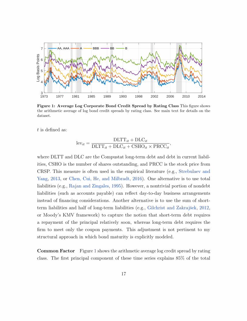
Figure 1: Average Log Corporate Bond Credit Spread by Rating Class This figure showsthe arithmetic average of log bond credit spreads by rating class. See main text for details on thedataset.
t is defined as:
levit =DLTTit + DLCit
DLTTit + DLCit + CSHOit × PRCCit
,
where DLTT and DLC are the Compustat long-term debt and debt in current liabil-
ities, CSHO is the number of shares outstanding, and PRCC is the stock price from
CRSP. This measure is often used in the empirical literature (e.g., Strebulaev and
Yang, 2013, or Chen, Cui, He, and Milbradt, 2016). One alternative is to use total
liabilities (e.g., Rajan and Zingales, 1995). However, a nontrivial portion of nondebt
liabilities (such as accounts payable) can reflect day-to-day business arrangements
instead of financing considerations. Another alternative is to use the sum of short-
term liabilities and half of long-term liabilities (e.g., Gilchrist and Zakrajsek, 2012,
or Moody’s KMV framework) to capture the notion that short-term debt requires
a repayment of the principal relatively soon, whereas long-term debt requires the
firm to meet only the coupon payments. This adjustment is not pertinent to my
structural approach in which bond maturity is explicitly modeled.
Common Factor Figure 1 shows the arithmetic average log credit spread by rating
class. The first principal component of these time series explains 85% of the total
17
log(cs) lev log(σE) log(σE,A) log(σE,I)
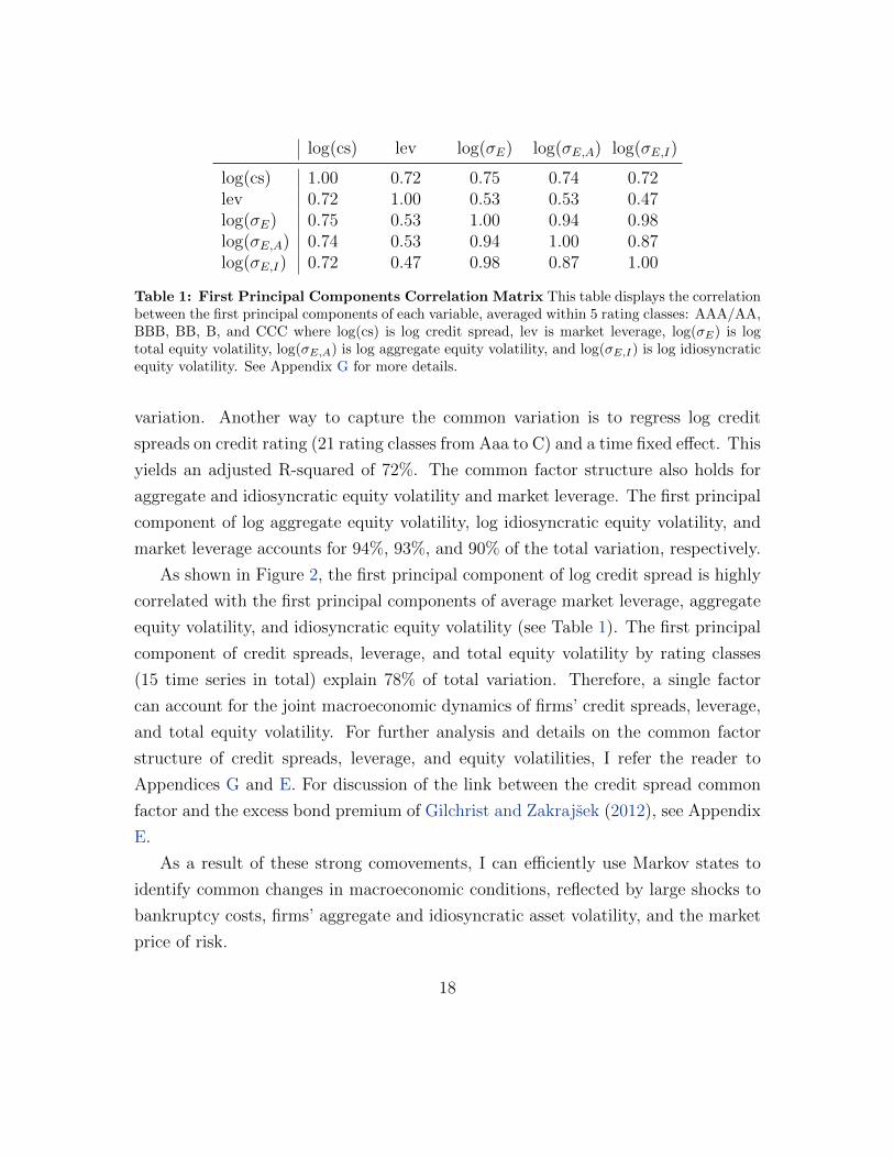
log(cs) 1.00 0.72 0.75 0.74 0.72lev 0.72 1.00 0.53 0.53 0.47log(σE) 0.75 0.53 1.00 0.94 0.98log(σE,A) 0.74 0.53 0.94 1.00 0.87log(σE,I) 0.72 0.47 0.98 0.87 1.00
Table 1: First Principal Components Correlation Matrix This table displays the correlationbetween the first principal components of each variable, averaged within 5 rating classes: AAA/AA,BBB, BB, B, and CCC where log(cs) is log credit spread, lev is market leverage, log(σE) is logtotal equity volatility, log(σE,A) is log aggregate equity volatility, and log(σE,I) is log idiosyncraticequity volatility. See Appendix G for more details.
variation. Another way to capture the common variation is to regress log credit
spreads on credit rating (21 rating classes from Aaa to C) and a time fixed effect. This
yields an adjusted R-squared of 72%. The common factor structure also holds for
aggregate and idiosyncratic equity volatility and market leverage. The first principal
component of log aggregate equity volatility, log idiosyncratic equity volatility, and
market leverage accounts for 94%, 93%, and 90% of the total variation, respectively.
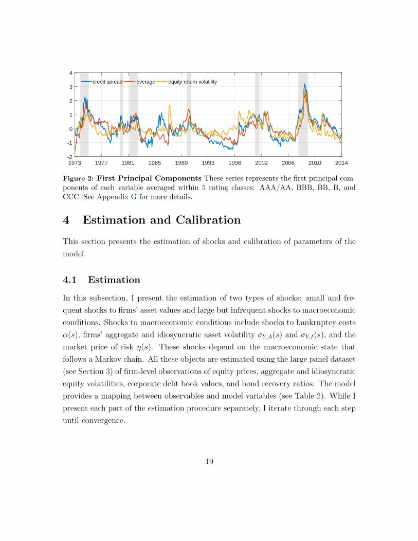
As shown in Figure 2, the first principal component of log credit spread is highly
correlated with the first principal components of average market leverage, aggregate
equity volatility, and idiosyncratic equity volatility (see Table 1). The first principal
component of credit spreads, leverage, and total equity volatility by rating classes
(15 time series in total) explain 78% of total variation. Therefore, a single factor
can account for the joint macroeconomic dynamics of firms’ credit spreads, leverage,
and total equity volatility. For further analysis and details on the common factor
structure of credit spreads, leverage, and equity volatilities, I refer the reader to
Appendices G and E. For discussion of the link between the credit spread common
factor and the excess bond premium of Gilchrist and Zakrajsek (2012), see Appendix
E.
As a result of these strong comovements, I can efficiently use Markov states to
identify common changes in macroeconomic conditions, reflected by large shocks to
bankruptcy costs, firms’ aggregate and idiosyncratic asset volatility, and the market
price of risk.
18
1973 1977 1981 1985 1989 1993 1998 2002 2006 2010 2014-2
-1
0
1
2
3
4
credit spread leverage equity return volatility
Figure 2: First Principal Components These series represents the first principal com-ponents of each variable averaged within 5 rating classes: AAA/AA, BBB, BB, B, andCCC. See Appendix G for more details.
4 Estimation and Calibration
This section presents the estimation of shocks and calibration of parameters of the
model.
4.1 Estimation
In this subsection, I present the estimation of two types of shocks: small and fre-
quent shocks to firms’ asset values and large but infrequent shocks to macroeconomic
conditions. Shocks to macroeconomic conditions include shocks to bankruptcy costs
α(s), firms’ aggregate and idiosyncratic asset volatility σY,A(s) and σY,I(s), and the
market price of risk η(s). These shocks depend on the macroeconomic state that
follows a Markov chain. All these objects are estimated using the large panel dataset
(see Section 3) of firm-level observations of equity prices, aggregate and idiosyncratic
equity volatilities, corporate debt book values, and bond recovery ratios. The model
provides a mapping between observables and model variables (see Table 2). While I
present each part of the estimation procedure separately, I iterate through each step
until convergence.
19
observations model variables
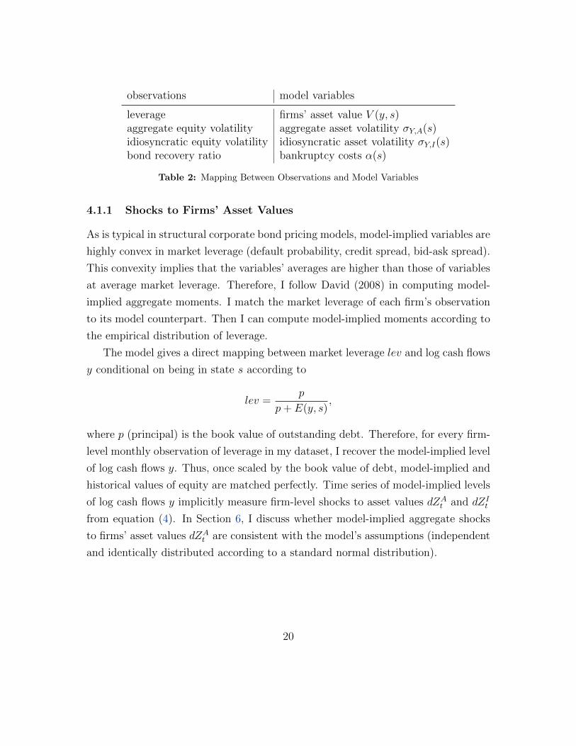
leverage firms’ asset value V (y, s)aggregate equity volatility aggregate asset volatility σY,A(s)idiosyncratic equity volatility idiosyncratic asset volatility σY,I(s)bond recovery ratio bankruptcy costs α(s)
Table 2: Mapping Between Observations and Model Variables
4.1.1 Shocks to Firms’ Asset Values
As is typical in structural corporate bond pricing models, model-implied variables are
highly convex in market leverage (default probability, credit spread, bid-ask spread).
This convexity implies that the variables’ averages are higher than those of variables
at average market leverage. Therefore, I follow David (2008) in computing model-
implied aggregate moments. I match the market leverage of each firm’s observation
to its model counterpart. Then I can compute model-implied moments according to
the empirical distribution of leverage.
The model gives a direct mapping between market leverage lev and log cash flows
y conditional on being in state s according to
lev =p
p+ E(y, s),
where p (principal) is the book value of outstanding debt. Therefore, for every firm-
level monthly observation of leverage in my dataset, I recover the model-implied level
of log cash flows y. Thus, once scaled by the book value of debt, model-implied and
historical values of equity are matched perfectly. Time series of model-implied levels
of log cash flows y implicitly measure firm-level shocks to asset values dZAt and dZI
t
from equation (4). In Section 6, I discuss whether model-implied aggregate shocks
to firms’ asset values dZAt are consistent with the model’s assumptions (independent
and identically distributed according to a standard normal distribution).
20
4.1.2 Shocks to Macroeconomic Conditions
Aggregate and Idiosyncratic Asset Volatility The stochastic processes for
firm’s asset volatilities are estimated for two types of firms: investment- and
speculative-grade firms. This separation is useful to generate predictions for the
financial indicators in the cross-section. Estimating the stochastic process for each
firm is unfeasible. Therefore, type-specific volatilities drive the dynamics of each firm
of that type, and the model is solved for each firm’s type, not for each firm. A firm
that is speculative-grade has a rating lower than Baa from Moody’s Investors Ser-
vice, a rating lower than BBB from Standard & Poor’s, or both. Firms with ratings
of Baa, BBB or higher are termed investment-grade. The relationship between firm
i’s aggregate asset volatility σiY,A(s) and its type j aggregate asset volatility σjY,A(s)
is given by:
log(σiY,A(s)
)= log
(σjY,A(s)
)+ εi (8)
where εi is independent and identically distributed measurement noise. The same
holds for idiosyncratic volatility.
While in the dataset a firm might move across rating classes, the model assumes
that an investment-grade firm never becomes speculative-grade, and vice versa. In-
troducing this feature is relatively unfeasible with Markov states, as it would expo-
nentially increase the amount of states required to solve the model.5 However, in
the estimation procedure, if an investment-grade firm in month t is downgraded to
speculative-grade in month t + 1, its observations contribute to the representative
investment-grade firm in month t and to the representative speculative-grade firm in
month t+ 1.
Using Ito’s Lemma, the model implies the following relationships:
σE,A(y, s)E(y, s) = E ′(y, s)σY,A(s),
σE,I(y, s)E(y, s) = E ′(y, s)σY,I(s),
5Currently, a firm of type j ∈ J can transition to S states in the next period. With this feature,a firm of type j ∈ J could transition to J × S states in the next period.
21
where Es(y, s) is the solution to the system of ODEs in equation (7), and σE,A(y|s)and σE,I(y|s) are the aggregate and idiosyncratic equity volatility of a firm with log
asset return y in state s. Thus, I can estimate firm i’s asset volatilities σiY,A(t|st) and
σiY,I(t|st) given observed values for equity volatilities σiE,A(t) and σiE,I(t) according
to
σiY,A(t|st) =Ej(yit, st)σ
iE,A(t)
Ej,′(yit, st),
σiY,I(t|st) =Ej(yit, st)σ
iE,I(t)
Ej,′(yit, st),
for every firm i, type j, time t, and state s.6 Section 3 details how observations of
aggregate and idiosyncratic equity volatility are constructed. From equation (8) it
follows that σjY,A(t|s) and σjY,I(t|s) can be estimated according to
log(σjY,A(t|s)
)=
1
N jt
∑i∈I(j,t)
log(σiY,A(t|s)
), (9)
log(σjY,I(t|s)
)=
1
N jt
∑i∈I(j,t)
log(σiY,I(t|s)
), (10)
for every type j, time t, and state s, where N jt is the amount of firms of type j at
time t, and I(j, t) is the set of firms of type j at time t.
Volatility States The above estimates are conditional on being in a state s at
each time t. Given the insights from Section 3 that equity volatilities, credit spreads,
and leverage comove, I use model-implied observations of asset volatilities to iden-
6Note that the estimate of aggregate equity volatility from CRSP at time t must be adjustedfor the size of the jump in equity value from the transition between state st−1 to state st. Moreprecisely,
σiE,A(t) =
√(viE,A(t)
)2−(Est(y)/Est−1
(y)− 1)2/21,
where viE,A(t) is the equity return aggregate volatility of firm i at time t described in Section 3.This adjustment turns out to be relatively insignificant.
22

tify fluctuations in macroeconomic states. This method identifies movements in the
macroeconomic state, but does not impose anything on the correlations between
state-dependent variables. Markovian states are estimated using the Baum-Welch
algorithm for hidden Markov models:
1. Initiate with values for the Markov chain M =σjY,A(s), σjY,I(s), ζP
.
2. Solve the structural model and estimate Y =σjY,A(t|s), σjY,I(t|s)
.
3. Identify the state st at each time t by maximizing the likelihood of being in
state s at time t, given the whole dataset Y (see Appendix C).
4. Get new estimates of aggregate and idiosyncratic asset volatilities
log(σjY,A(s)
)=
∑Tt=1 log
(σjY,A(t|s)
)1 st = s∑T
t=1 1 st = s
log(σjY,I(s)
)=
∑Tt=1 log
(σjY,I(t|s)
)1 st = s∑T
t=1 1 st = s.
5. Update transition intensities ζss′
P with the empirical discrete transition proba-
bilities πss′
given by
πss′=
∑T−1t=1 1 st = s1 st+1 = s′∑T
t=1 1 st = s
for all s, s′. See Appendix D for more details.
6. Iterate on 2-5 until convergence.
This estimation procedure is dependent on initial guesses forM and the number
of states. However, it is easy to check how well the estimation procedure approxi-
mates the continuous time series of estimated volatilities with the Markov chain by
looking at the difference betweenσjY,A(t|st), σjY,I(t|st)
Tt=1
andσjY,A(st), σ
jY,I(st)
Tt=1
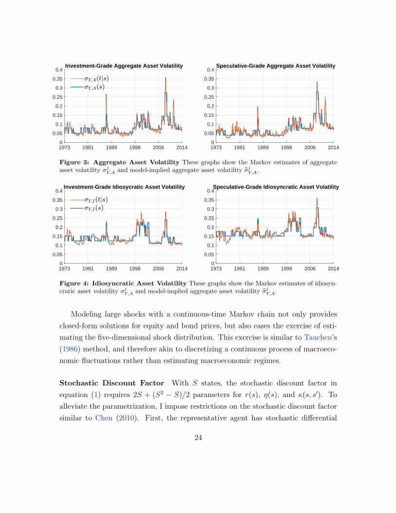
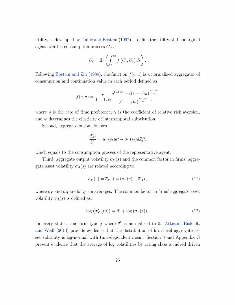
in Figures 3 and 4. Increasing the number of states improves the fit, but at the cost
of more transition probabilities to estimate. Likelihood plateaus at 8 states.
23
1973 1981 1989 1998 2006 20140
0.05
0.1
0.15
0.2
0.25
0.3
0.35
0.4Investment-Grade Aggregate Asset Volatility
<Y;A(tjs)<Y;A(s)
1973 1981 1989 1998 2006 20140
0.05
0.1
0.15
0.2
0.25
0.3
0.35
0.4Speculative-Grade Aggregate Asset Volatility
Figure 3: Aggregate Asset Volatility These graphs show the Markov estimates of aggregateasset volatility σjY,A and model-implied aggregate asset volatility σjY,A.
1973 1981 1989 1998 2006 20140
0.05
0.1
0.15
0.2
0.25
0.3
0.35
0.4Investment-Grade Idiosycratic Asset Volatility
<Y;I(tjs)<Y;I(s)
1973 1981 1989 1998 2006 20140
0.05
0.1
0.15
0.2
0.25
0.3
0.35
0.4Speculative-Grade Idiosyncratic Asset Volatility
Figure 4: Idiosyncratic Asset Volatility These graphs show the Markov estimates of idiosyn-cratic asset volatility σjY,A and model-implied aggregate asset volatility σjY,A.
Modeling large shocks with a continuous-time Markov chain not only provides
closed-form solutions for equity and bond prices, but also eases the exercise of esti-
mating the five-dimensional shock distribution. This exercise is similar to Tauchen’s
(1986) method, and therefore akin to discretizing a continuous process of macroeco-
nomic fluctuations rather than estimating macroeconomic regimes.
Stochastic Discount Factor With S states, the stochastic discount factor in
equation (1) requires 2S + (S2 − S)/2 parameters for r(s), η(s), and κ(s, s′). To
alleviate the parametrization, I impose restrictions on the stochastic discount factor
similar to Chen (2010). First, the representative agent has stochastic differential
24
utility, as developed by Duffie and Epstein (1992). I define the utility of the marginal
agent over his consumption process C as
Ut = Et(∫ ∞
t
f (Cs, Us) ds
).
Following Epstein and Zin (1989), the function f(c, u) is a normalized aggregator of
consumption and continuation value in each period defined as
f(c, u) =ρ
1− 1/ψ
c1−1/ψ − ((1− γ)u)1−1/ψ1−γ
((1− γ)u)1−1/ψ1−γ −1
where ρ is the rate of time preference, γ is the coefficient of relative risk aversion,
and ψ determines the elasticity of intertemporal substitution.
Second, aggregate output follows
dYtYt
= µY (st)dt+ σY (st)dZAt ,
which equals to the consumption process of the representative agent.
Third, aggregate output volatility σY (s) and the common factor in firms’ aggre-
gate asset volatility σA(s) are related according to
σY (s) = sσY + ϕ (σA(s)− sσA) , (11)
where sσY and sσA are long-run averages. The common factor in firms’ aggregate asset
volatility σA(s) is defined as:
log(σjY,A(s)
)= θj + log (σA(s)) , (12)
for every state s and firm type j where θ1 is normalized to 0. Atkeson, Eisfeldt,
and Weill (2013) provide evidence that the distribution of firm-level aggregate as-
set volatility is log-normal with time-dependent mean. Section 3 and Appendix G
present evidence that the average of log volatilities by rating class is indeed driven
25
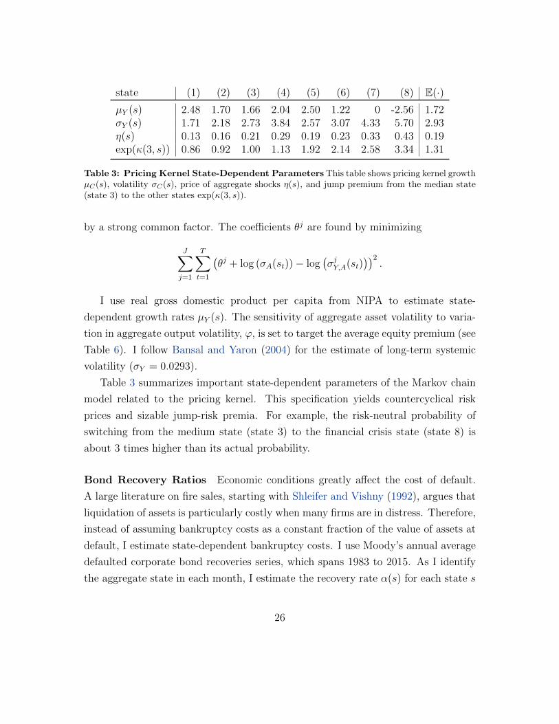
state (1) (2) (3) (4) (5) (6) (7) (8) E(·)µY (s) 2.48 1.70 1.66 2.04 2.50 1.22 0 -2.56 1.72σY (s) 1.71 2.18 2.73 3.84 2.57 3.07 4.33 5.70 2.93η(s) 0.13 0.16 0.21 0.29 0.19 0.23 0.33 0.43 0.19exp(κ(3, s)) 0.86 0.92 1.00 1.13 1.92 2.14 2.58 3.34 1.31
Table 3: Pricing Kernel State-Dependent Parameters This table shows pricing kernel growthµC(s), volatility σC(s), price of aggregate shocks η(s), and jump premium from the median state(state 3) to the other states exp(κ(3, s)).
by a strong common factor. The coefficients θj are found by minimizing
J∑j=1
T∑t=1
(θj + log (σA(st))− log
(σjY,A(st)
))2.
I use real gross domestic product per capita from NIPA to estimate state-
dependent growth rates µY (s). The sensitivity of aggregate asset volatility to varia-
tion in aggregate output volatility, ϕ, is set to target the average equity premium (see
Table 6). I follow Bansal and Yaron (2004) for the estimate of long-term systemic
volatility (sσY = 0.0293).
Table 3 summarizes important state-dependent parameters of the Markov chain
model related to the pricing kernel. This specification yields countercyclical risk
prices and sizable jump-risk premia. For example, the risk-neutral probability of
switching from the medium state (state 3) to the financial crisis state (state 8) is
about 3 times higher than its actual probability.
Bond Recovery Ratios Economic conditions greatly affect the cost of default.
A large literature on fire sales, starting with Shleifer and Vishny (1992), argues that
liquidation of assets is particularly costly when many firms are in distress. Therefore,
instead of assuming bankruptcy costs as a constant fraction of the value of assets at
default, I estimate state-dependent bankruptcy costs. I use Moody’s annual average
defaulted corporate bond recoveries series, which spans 1983 to 2015. As I identify
the aggregate state in each month, I estimate the recovery rate α(s) for each state s
26
according to
α(s) =
∑Tt=1 rect × vb(st)1 st = s∑T
t=1 1 st = s,
where rect is Moody’s defaulted corporate bond recovery ratio at time t and vb(s)
is the value of the unlevered firm at the endogenous bankruptcy level divided by the
bond principal value p in state s. Moody measures recovery ratios using post-default
trading prices. Therefore, assuming that post-default prices are the bid prices at
which investors are selling, we have that
α(s) = αL(s) + β(αH(s)− αL(s)
),
where αH(s) and αL(s) are the recovery rate in state s for bond investors of H- and
L-type, respectively. The estimated average recovery ratio over the whole sample
E [α(s)] is about 45%, in line with the estimate of bankruptcy recovery by Chen
(2010). The lowest α(s) is equal to 33% and corresponds to the state of the 2008–2009
financial crisis. Note that this recovery ratio is different from the ultimate recovery
of the bond after resolution of bankruptcy. With an average resolution period of
1.37 years, according to the Moody’s default and recovery database, and an excess
return of 23% on a portfolio of all defaulted bonds over 1987–2011 estimated by He
and Milbradt (2014), the average ultimate recovery rate is about 70%. Estimating
separate recovery ratios for each firm’s type does not yield significant differences.
4.2 Calibration
I follow Bansal and Yaron (2004) for the parameters of risk aversion and intertem-
poral substitution, with γ = 7.5 and ψ = 1.5. With a discount rate ρ equal to 0.02, I
get an average risk-free interest rate of 2%. Note that this is close to the lower bond
for the firm’s asset value vs in (3) to exist, as the risk-free discount rate must be high
enough relative to the drift of firms’ asset value µY of investment-grade firms. The
calibration of µY is discussed below.
27
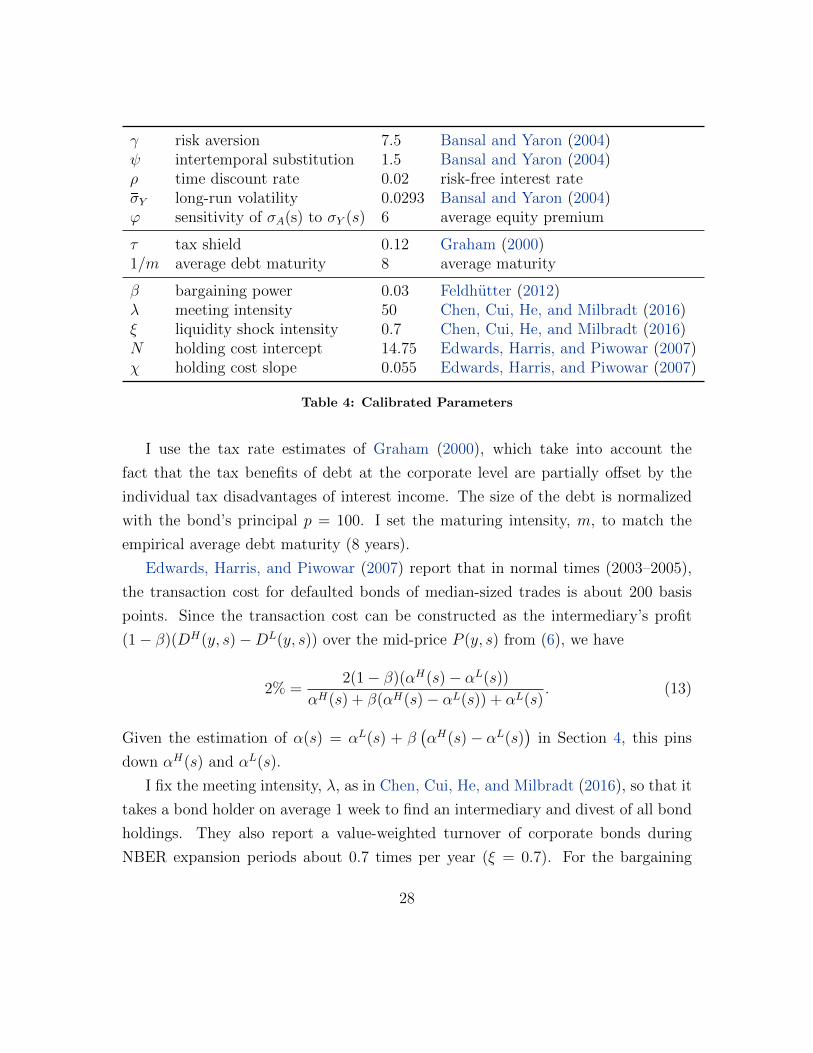
γ risk aversion 7.5 Bansal and Yaron (2004)ψ intertemporal substitution 1.5 Bansal and Yaron (2004)ρ time discount rate 0.02 risk-free interest ratesσY long-run volatility 0.0293 Bansal and Yaron (2004)ϕ sensitivity of σA(s) to σY (s) 6 average equity premium
τ tax shield 0.12 Graham (2000)1/m average debt maturity 8 average maturity
β bargaining power 0.03 Feldhutter (2012)λ meeting intensity 50 Chen, Cui, He, and Milbradt (2016)ξ liquidity shock intensity 0.7 Chen, Cui, He, and Milbradt (2016)N holding cost intercept 14.75 Edwards, Harris, and Piwowar (2007)χ holding cost slope 0.055 Edwards, Harris, and Piwowar (2007)
Table 4: Calibrated Parameters
I use the tax rate estimates of Graham (2000), which take into account the
fact that the tax benefits of debt at the corporate level are partially offset by the
individual tax disadvantages of interest income. The size of the debt is normalized
with the bond’s principal p = 100. I set the maturing intensity, m, to match the
empirical average debt maturity (8 years).
Edwards, Harris, and Piwowar (2007) report that in normal times (2003–2005),
the transaction cost for defaulted bonds of median-sized trades is about 200 basis
points. Since the transaction cost can be constructed as the intermediary’s profit
(1− β)(DH(y, s)−DL(y, s)) over the mid-price P (y, s) from (6), we have
2% =2(1− β)(αH(s)− αL(s))
αH(s) + β(αH(s)− αL(s)) + αL(s). (13)
Given the estimation of α(s) = αL(s) + β(αH(s)− αL(s)
)in Section 4, this pins
down αH(s) and αL(s).
I fix the meeting intensity, λ, as in Chen, Cui, He, and Milbradt (2016), so that it
takes a bond holder on average 1 week to find an intermediary and divest of all bond
holdings. They also report a value-weighted turnover of corporate bonds during
NBER expansion periods about 0.7 times per year (ξ = 0.7). For the bargaining
28
power allocation between dealers and investors, β, I follow Feldhutter (2012).
Edwards, Harris, and Piwowar (2007) use the Trade Reporting and Compliance
Engine bond price database from January 2003 to January 2005 to estimate reported
bid-ask spreads for different firm ratings and trading sizes. I calibrate χ and N to
match the average implied bid-ask spreads and their measurement of bid-ask spreads
for investment- and speculative-grade bonds for a transaction of median size during
that period. See Figure 10 for model-implied bid-ask spreads from 2002 to 2009.
The coupon payment c is set such that, on average, corporate bonds are issued
at par value. That is, the coupon payment c of firms of type j satisfies the following
condition:
1
T
T∑t=1
DHj (yj, st) = p
where DHj (yj, s) is the value of a bond of type j for the H-type investor in state s, yj
is the asset return level corresponding to the average leverage level of firms of type
j, and st is the state identified during the estimation procedure.
The drift of firms’ asset values under the physical measure essentially affects the
overall match between default rates, credit spreads, and leverage. While important
for the quantitative performance of a credit risk model, no consistent measurement
has been agreed upon or consensus reached in the literature by which a wide range
of values is used.7 Therefore, I calibrate asset return drift by firm type to target
Moody’s historical 8-year average cumulative default rate (see Figure 5). Huang
and Huang (2012) reveal that structural models typically imply a much steeper term
structure of cumulative default rates than reflected in the data. Extensions of the
model, such as introducing jumps in firms’ asset values, are likely to help in that
dimension, but accurately matching the term structure of cumulative default rates
is beyond the scope of this paper.
7He and Milbradt (2014): 0.018; Bhamra, Kuehn, and Strebulaev (2010): -0.04 and 0.08, with2 aggregate states; Chen (2010): from -0.10 to 0.11, with 9 aggregate states; Leland (2006): 0.045.
29
2 4 6 8 10 12 14year
0
0.1
0.2
0.3
0.4
0.5
cum
ulat
ive
defa
ult model investment grade
data investment grademodel speculative gradedata speculative grade
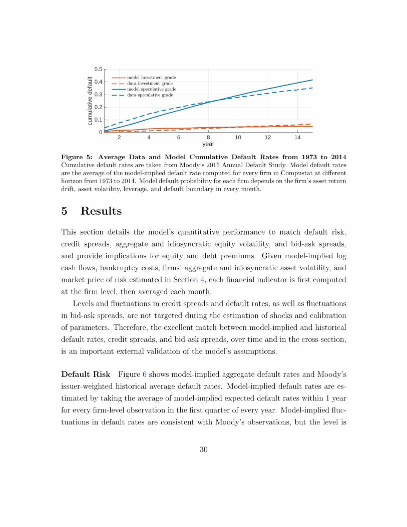
Figure 5: Average Data and Model Cumulative Default Rates from 1973 to 2014Cumulative default rates are taken from Moody’s 2015 Annual Default Study. Model default ratesare the average of the model-implied default rate computed for every firm in Compustat at differenthorizon from 1973 to 2014. Model default probability for each firm depends on the firm’s asset returndrift, asset volatility, leverage, and default boundary in every month.
5 Results
This section details the model’s quantitative performance to match default risk,
credit spreads, aggregate and idiosyncratic equity volatility, and bid-ask spreads,
and provide implications for equity and debt premiums. Given model-implied log
cash flows, bankruptcy costs, firms’ aggregate and idiosyncratic asset volatility, and
market price of risk estimated in Section 4, each financial indicator is first computed
at the firm level, then averaged each month.
Levels and fluctuations in credit spreads and default rates, as well as fluctuations
in bid-ask spreads, are not targeted during the estimation of shocks and calibration
of parameters. Therefore, the excellent match between model-implied and historical
default rates, credit spreads, and bid-ask spreads, over time and in the cross-section,
is an important external validation of the model’s assumptions.
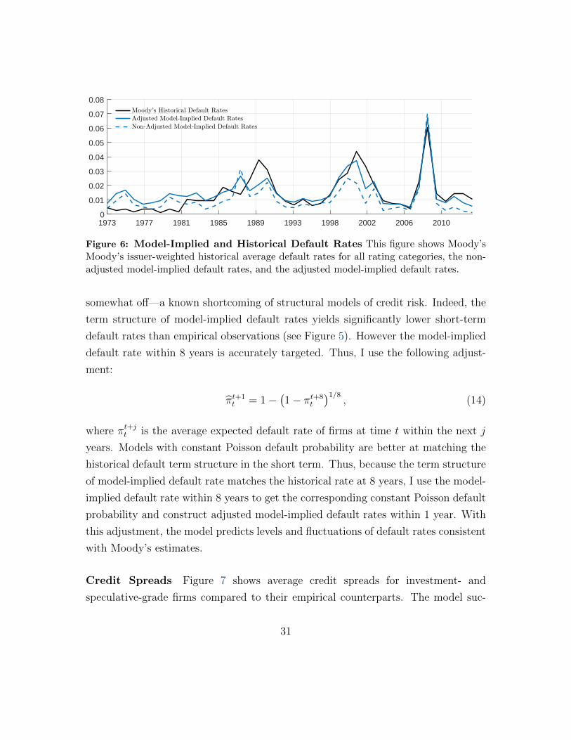
Default Risk Figure 6 shows model-implied aggregate default rates and Moody’s
issuer-weighted historical average default rates. Model-implied default rates are es-
timated by taking the average of model-implied expected default rates within 1 year
for every firm-level observation in the first quarter of every year. Model-implied fluc-
tuations in default rates are consistent with Moody’s observations, but the level is
30
1973 1977 1981 1985 1989 1993 1998 2002 2006 20100
0.01
0.02
0.03
0.04
0.05
0.06
0.07
0.08Moody's Historical Default Rates
Adjusted Model-Implied Default Rates
Non-Adjusted Model-Implied Default Rates
Figure 6: Model-Implied and Historical Default Rates This figure shows Moody’sMoody’s issuer-weighted historical average default rates for all rating categories, the non-adjusted model-implied default rates, and the adjusted model-implied default rates.
somewhat off—a known shortcoming of structural models of credit risk. Indeed, the
term structure of model-implied default rates yields significantly lower short-term
default rates than empirical observations (see Figure 5). However the model-implied
default rate within 8 years is accurately targeted. Thus, I use the following adjust-
ment:
πt+1t = 1−
(1− πt+8
t
)1/8, (14)
where πt+jt is the average expected default rate of firms at time t within the next j
years. Models with constant Poisson default probability are better at matching the
historical default term structure in the short term. Thus, because the term structure
of model-implied default rate matches the historical rate at 8 years, I use the model-
implied default rate within 8 years to get the corresponding constant Poisson default
probability and construct adjusted model-implied default rates within 1 year. With
this adjustment, the model predicts levels and fluctuations of default rates consistent
with Moody’s estimates.
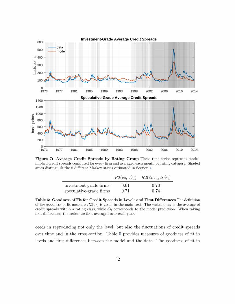
Credit Spreads Figure 7 shows average credit spreads for investment- and
speculative-grade firms compared to their empirical counterparts. The model suc-
31
1973 1977 1981 1985 1989 1993 1998 2002 2006 2010 20140
100
200
300
400
500
600
basi
s po
ints
Investment-Grade Average Credit Spreads
datamodel
1973 1977 1981 1985 1989 1993 1998 2002 2006 2010 20140
200
400
600
800
1000
1200
1400
basi
s po
ints
Speculative-Grade Average Credit Spreads
Figure 7: Average Credit Spreads by Rating Group These time series represent model-implied credit spreads computed for every firm and averaged each month by rating category. Shadedareas distinguish the 8 different Markov states estimated in Section 4.
R2(cst, cst) R2(∆cst,∆cst)
investment-grade firms 0.61 0.70speculative-grade firms 0.71 0.74
Table 5: Goodness of Fit for Credit Spreads in Levels and First Differences The definitionof the goodness of fit measure R2(·, ·) is given in the main text. The variable cst is the average ofcredit spreads within a rating class, while cst corresponds to the model prediction. When takingfirst differences, the series are first averaged over each year.
ceeds in reproducing not only the level, but also the fluctuations of credit spreads
over time and in the cross-section. Table 5 provides measures of goodness of fit in
levels and first differences between the model and the data. The goodness of fit in
32
1973 1981 1989 1998 2006 20140
0.2
0.4
0.6
0.8
1Investment-Grade Aggregate Equity Volatility
vE;A(t)<E;A(t)
1973 1981 1989 1998 2006 20140
0.2
0.4
0.6
0.8
1Speculative-Grade Aggregate Equity Volatility
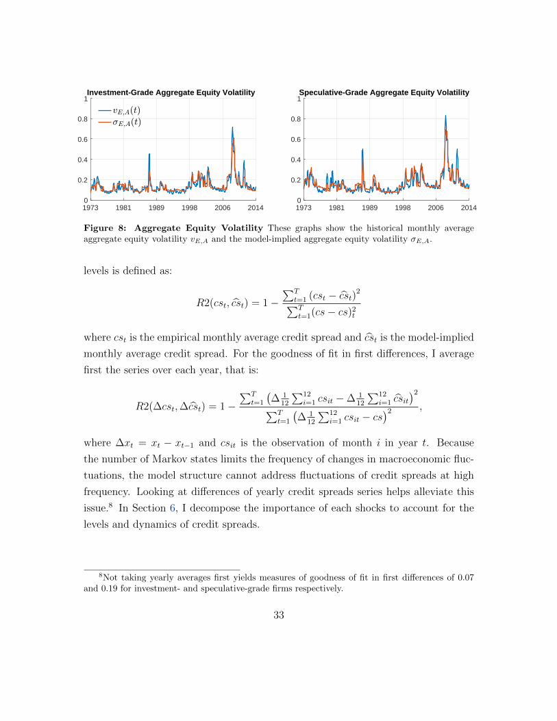
Figure 8: Aggregate Equity Volatility These graphs show the historical monthly averageaggregate equity volatility vE,A and the model-implied aggregate equity volatility σE,A.
levels is defined as:
R2(cst, cst) = 1−∑T
t=1 (cst − cst)2∑Tt=1(cs− scs)2t
where cst is the empirical monthly average credit spread and cst is the model-implied
monthly average credit spread. For the goodness of fit in first differences, I average
first the series over each year, that is:
R2(∆cst,∆cst) = 1−∑T
t=1
(∆ 1
12
∑12i=1 csit −∆ 1
12
∑12i=1 csit
)2∑Tt=1
(∆ 1
12
∑12i=1 csit − scs
)2 ,
where ∆xt = xt − xt−1 and csit is the observation of month i in year t. Because
the number of Markov states limits the frequency of changes in macroeconomic fluc-
tuations, the model structure cannot address fluctuations of credit spreads at high
frequency. Looking at differences of yearly credit spreads series helps alleviate this
issue.8 In Section 6, I decompose the importance of each shocks to account for the
levels and dynamics of credit spreads.
8Not taking yearly averages first yields measures of goodness of fit in first differences of 0.07and 0.19 for investment- and speculative-grade firms respectively.
33
1973 1981 1989 1998 2006 20140
0.2
0.4
0.6
0.8
1Investment-Grade Idiosycratic Equity Volatility
vE;I(t)<E;I(t)
1973 1981 1989 1998 2006 20140
0.2
0.4
0.6
0.8
1Speculative-Grade Idiosyncratic Equity Volatility
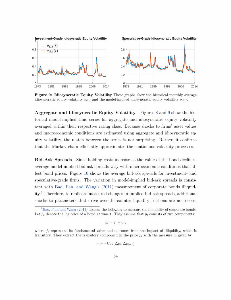
Figure 9: Idiosyncratic Equity Volatility These graphs show the historical monthly averageidiosyncratic equity volatility vE,I and the model-implied idiosyncratic equity volatility σE,I .
Aggregate and Idiosyncratic Equity Volatility Figures 8 and 9 show the his-
torical model-implied time series for aggregate and idiosyncratic equity volatility
averaged within their respective rating class. Because shocks to firms’ asset values
and macroeconomic conditions are estimated using aggregate and idiosyncratic eq-
uity volatility, the match between the series is not surprising. Rather, it confirms
that the Markov chain efficiently approximates the continuous volatility processes.
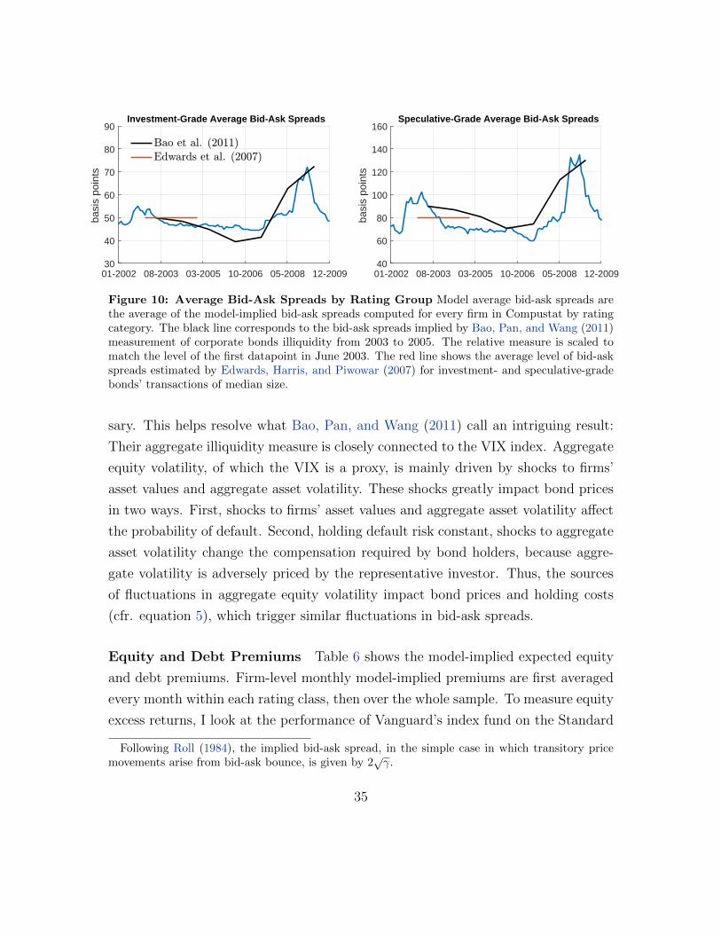
Bid-Ask Spreads Since holding costs increase as the value of the bond declines,
average model-implied bid-ask spreads vary with macroeconomic conditions that af-
fect bond prices. Figure 10 shows the average bid-ask spreads for investment- and
speculative-grade firms. The variation in model-implied bid-ask spreads is consis-
tent with Bao, Pan, and Wang’s (2011) measurement of corporate bonds illiquid-
ity.9 Therefore, to replicate measured changes in implied bid-ask spreads, additional
shocks to parameters that drive over-the-counter liquidity frictions are not neces-
9Bao, Pan, and Wang (2011) assume the following to measure the illiquidity of corporate bonds.Let pt denote the log price of a bond at time t. They assume that pt consists of two components:
pt = ft + ut,
where ft represents its fundamental value and ut comes from the impact of illiquidity, which istransitory. They extract the transitory component in the price pt with the measure γt given by
γt = −Cov(∆pt,∆pt+1).
34
01-2002 08-2003 03-2005 10-2006 05-2008 12-200930
40
50
60
70
80
90
basi
s po
ints
Investment-Grade Average Bid-Ask Spreads
Bao et al. (2011)Edwards et al. (2007)
01-2002 08-2003 03-2005 10-2006 05-2008 12-200940
60
80
100
120
140
160
basi
s po
ints
Speculative-Grade Average Bid-Ask Spreads
Figure 10: Average Bid-Ask Spreads by Rating Group Model average bid-ask spreads arethe average of the model-implied bid-ask spreads computed for every firm in Compustat by ratingcategory. The black line corresponds to the bid-ask spreads implied by Bao, Pan, and Wang (2011)measurement of corporate bonds illiquidity from 2003 to 2005. The relative measure is scaled tomatch the level of the first datapoint in June 2003. The red line shows the average level of bid-askspreads estimated by Edwards, Harris, and Piwowar (2007) for investment- and speculative-gradebonds’ transactions of median size.
sary. This helps resolve what Bao, Pan, and Wang (2011) call an intriguing result:
Their aggregate illiquidity measure is closely connected to the VIX index. Aggregate
equity volatility, of which the VIX is a proxy, is mainly driven by shocks to firms’
asset values and aggregate asset volatility. These shocks greatly impact bond prices
in two ways. First, shocks to firms’ asset values and aggregate asset volatility affect
the probability of default. Second, holding default risk constant, shocks to aggregate
asset volatility change the compensation required by bond holders, because aggre-
gate volatility is adversely priced by the representative investor. Thus, the sources
of fluctuations in aggregate equity volatility impact bond prices and holding costs
(cfr. equation 5), which trigger similar fluctuations in bid-ask spreads.
Equity and Debt Premiums Table 6 shows the model-implied expected equity
and debt premiums. Firm-level monthly model-implied premiums are first averaged
every month within each rating class, then over the whole sample. To measure equity
excess returns, I look at the performance of Vanguard’s index fund on the Standard
Following Roll (1984), the implied bid-ask spread, in the simple case in which transitory pricemovements arise from bid-ask bounce, is given by 2
√γ.
35
equity premium bond premiummodel model data model
1973–2014 1987–2014 1987–2014 1973–2014
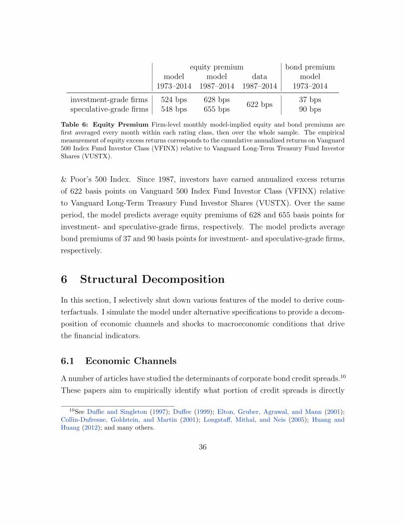
investment-grade firms 524 bps 628 bps622 bps
37 bpsspeculative-grade firms 548 bps 655 bps 90 bps
Table 6: Equity Premium Firm-level monthly model-implied equity and bond premiums arefirst averaged every month within each rating class, then over the whole sample. The empiricalmeasurement of equity excess returns corresponds to the cumulative annualized returns on Vanguard500 Index Fund Investor Class (VFINX) relative to Vanguard Long-Term Treasury Fund InvestorShares (VUSTX).
& Poor’s 500 Index. Since 1987, investors have earned annualized excess returns
of 622 basis points on Vanguard 500 Index Fund Investor Class (VFINX) relative
to Vanguard Long-Term Treasury Fund Investor Shares (VUSTX). Over the same
period, the model predicts average equity premiums of 628 and 655 basis points for
investment- and speculative-grade firms, respectively. The model predicts average
bond premiums of 37 and 90 basis points for investment- and speculative-grade firms,
respectively.
6 Structural Decomposition
In this section, I selectively shut down various features of the model to derive coun-
terfactuals. I simulate the model under alternative specifications to provide a decom-
position of economic channels and shocks to macroeconomic conditions that drive
the financial indicators.
6.1 Economic Channels
A number of articles have studied the determinants of corporate bond credit spreads.10
These papers aim to empirically identify what portion of credit spreads is directly
10See Duffie and Singleton (1997); Duffee (1999); Elton, Gruber, Agrawal, and Mann (2001);Collin-Dufresne, Goldstein, and Martin (2001); Longstaff, Mithal, and Neis (2005); Huang andHuang (2012); and many others.
36
Investment Grade Credit Spreads Decomposition
1973 1977 1981 1985 1989 1993 1998 2002 2006 2010 20140
20
40
60
80
100
%
Speculative Grade Credit Spreads Decomposition
1973 1977 1981 1985 1989 1993 1998 2002 2006 2010 20140
20
40
60
80
100
%
" Liquidity
" Risk Aversion
" Default Risk
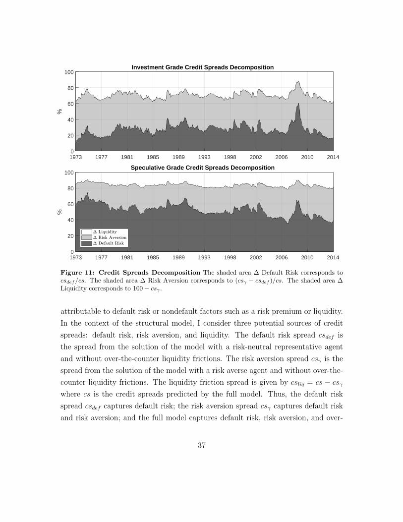
Figure 11: Credit Spreads Decomposition The shaded area ∆ Default Risk corresponds tocsdef/cs. The shaded area ∆ Risk Aversion corresponds to (csγ − csdef )/cs. The shaded area ∆Liquidity corresponds to 100− csγ .
attributable to default risk or nondefault factors such as a risk premium or liquidity.
In the context of the structural model, I consider three potential sources of credit
spreads: default risk, risk aversion, and liquidity. The default risk spread csdef is
the spread from the solution of the model with a risk-neutral representative agent
and without over-the-counter liquidity frictions. The risk aversion spread csγ is the
spread from the solution of the model with a risk averse agent and without over-the-
counter liquidity frictions. The liquidity friction spread is given by csliq = cs − csγwhere cs is the credit spreads predicted by the full model. Thus, the default risk
spread csdef captures default risk; the risk aversion spread csγ captures default risk
and risk aversion; and the full model captures default risk, risk aversion, and over-
37
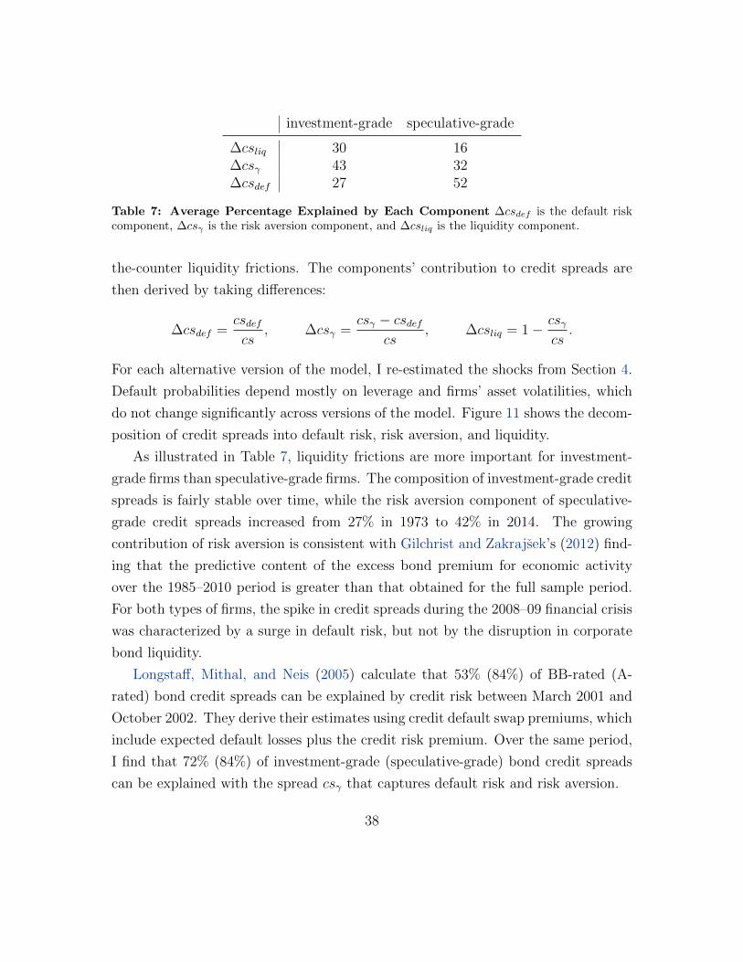
investment-grade speculative-grade
∆csliq 30 16∆csγ 43 32∆csdef 27 52
Table 7: Average Percentage Explained by Each Component ∆csdef is the default riskcomponent, ∆csγ is the risk aversion component, and ∆csliq is the liquidity component.
the-counter liquidity frictions. The components’ contribution to credit spreads are
then derived by taking differences:
∆csdef =csdefcs
, ∆csγ =csγ − csdef
cs, ∆csliq = 1− csγ
cs.
For each alternative version of the model, I re-estimated the shocks from Section 4.
Default probabilities depend mostly on leverage and firms’ asset volatilities, which
do not change significantly across versions of the model. Figure 11 shows the decom-
position of credit spreads into default risk, risk aversion, and liquidity.
As illustrated in Table 7, liquidity frictions are more important for investment-
grade firms than speculative-grade firms. The composition of investment-grade credit
spreads is fairly stable over time, while the risk aversion component of speculative-
grade credit spreads increased from 27% in 1973 to 42% in 2014. The growing
contribution of risk aversion is consistent with Gilchrist and Zakrajsek’s (2012) find-
ing that the predictive content of the excess bond premium for economic activity
over the 1985–2010 period is greater than that obtained for the full sample period.
For both types of firms, the spike in credit spreads during the 2008–09 financial crisis
was characterized by a surge in default risk, but not by the disruption in corporate
bond liquidity.
Longstaff, Mithal, and Neis (2005) calculate that 53% (84%) of BB-rated (A-
rated) bond credit spreads can be explained by credit risk between March 2001 and
October 2002. They derive their estimates using credit default swap premiums, which
include expected default losses plus the credit risk premium. Over the same period,
I find that 72% (84%) of investment-grade (speculative-grade) bond credit spreads
can be explained with the spread csγ that captures default risk and risk aversion.
38
Chen, Cui, He, and Milbradt (2016) find that the fraction of credit spreads that
can be explained without liquidity frictions starts at only 20% for Aaa/Aa-rated
bonds, and monotonically increases to about 67% for Ba-rated bonds for the period
starting in January 1994 and ending in June 2012. In contrast, I find that 71% (83%)
of credit spreads can be accounted for without liquidity friction for investment-grade
(speculative-grade) bond credit spreads over the same period. An important factor
in these differences resides in the measurement and inclusion of time-varying firms’
asset volatilities to explain the levels of credit spreads and bid-ask spreads instead
of time-varying parameters that drive over-the-counter liquidity frictions.
6.2 Aggregate Shocks to Firms’ Asset Value
Before presenting the shocks decomposition, it is important to understand that with-
out shocks to macroeconomic conditions, the model generates aggregate shocks to
firms’ asset values inconsistent with the model’s assumptions. This can be shown by
constructing a discrete approximation to aggregate shocks to firms’ asset volatility
dZAt from equation (4). For a representative firm of type j, I retrieve model-implied
levels of log cash flows yjt at time t following:
yjt =1
N jt
∑i∈I(j,t)
yit,
where N jt is the amount of firms of type j at time t and I(j, t) is the set of firms of
type j at time t. The approximation to dZAt is then given by:
∆ZAt =
1
J
J∑j=1
yjt − yjt−1 − µ
jY + 0.5σjY,A(st)
σjY,A(st),
where σjY,A(s) is the aggregate asset volatility of firms of type j in state s, and µjYis the drift of asset values of firms of type j (see equations 2 and 4). According to
the model, ∆ZAt should be identically and independently distributed according to
a standard normal distribution. In Figure 12, two graphs represent histograms of
39
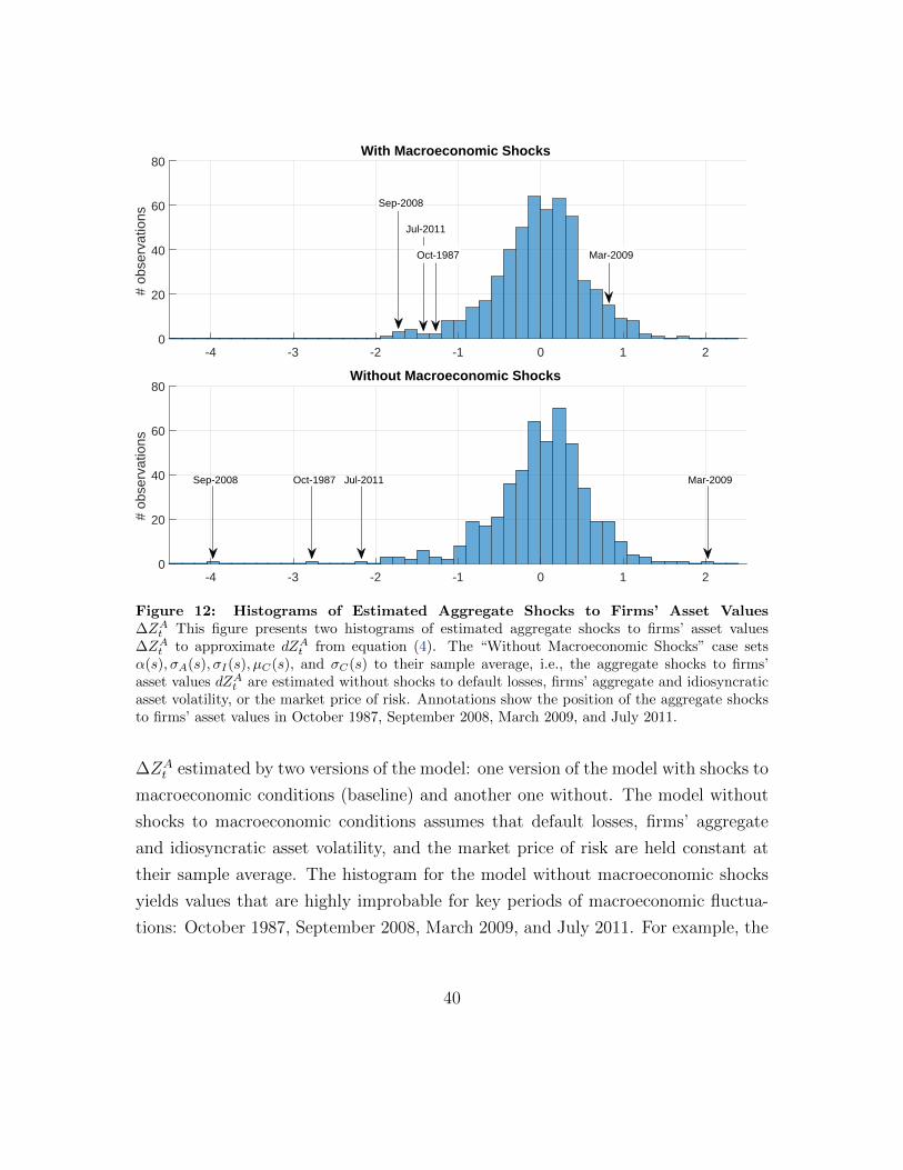
-4 -3 -2 -1 0 1 20
20
40
60
80
# ob
serv
atio
nsWith Macroeconomic Shocks
Jul-2011
Mar-2009
Sep-2008
Oct-1987
-4 -3 -2 -1 0 1 20
20
40
60
80
# ob
serv
atio
ns
Without Macroeconomic Shocks
Oct-1987Sep-2008 Mar-2009Jul-2011
Figure 12: Histograms of Estimated Aggregate Shocks to Firms’ Asset Values∆ZAt This figure presents two histograms of estimated aggregate shocks to firms’ asset values∆ZAt to approximate dZAt from equation (4). The “Without Macroeconomic Shocks” case setsα(s), σA(s), σI(s), µC(s), and σC(s) to their sample average, i.e., the aggregate shocks to firms’asset values dZAt are estimated without shocks to default losses, firms’ aggregate and idiosyncraticasset volatility, or the market price of risk. Annotations show the position of the aggregate shocksto firms’ asset values in October 1987, September 2008, March 2009, and July 2011.
∆ZAt estimated by two versions of the model: one version of the model with shocks to
macroeconomic conditions (baseline) and another one without. The model without
shocks to macroeconomic conditions assumes that default losses, firms’ aggregate
and idiosyncratic asset volatility, and the market price of risk are held constant at
their sample average. The histogram for the model without macroeconomic shocks
yields values that are highly improbable for key periods of macroeconomic fluctua-
tions: October 1987, September 2008, March 2009, and July 2011. For example, the
40
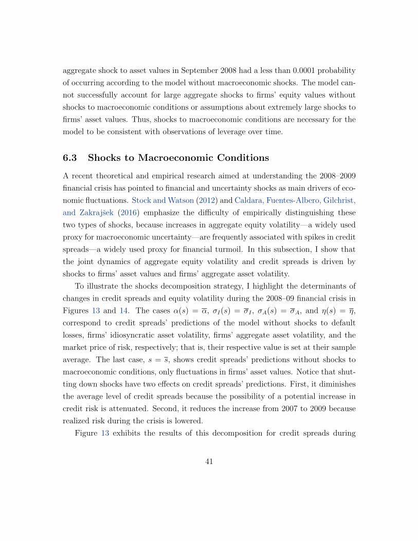
aggregate shock to asset values in September 2008 had a less than 0.0001 probability
of occurring according to the model without macroeconomic shocks. The model can-
not successfully account for large aggregate shocks to firms’ equity values without
shocks to macroeconomic conditions or assumptions about extremely large shocks to
firms’ asset values. Thus, shocks to macroeconomic conditions are necessary for the
model to be consistent with observations of leverage over time.
6.3 Shocks to Macroeconomic Conditions
A recent theoretical and empirical research aimed at understanding the 2008–2009
financial crisis has pointed to financial and uncertainty shocks as main drivers of eco-
nomic fluctuations. Stock and Watson (2012) and Caldara, Fuentes-Albero, Gilchrist,
and Zakrajsek (2016) emphasize the difficulty of empirically distinguishing these
two types of shocks, because increases in aggregate equity volatility—a widely used
proxy for macroeconomic uncertainty—are frequently associated with spikes in credit
spreads—a widely used proxy for financial turmoil. In this subsection, I show that
the joint dynamics of aggregate equity volatility and credit spreads is driven by
shocks to firms’ asset values and firms’ aggregate asset volatility.
To illustrate the shocks decomposition strategy, I highlight the determinants of
changes in credit spreads and equity volatility during the 2008–09 financial crisis in
Figures 13 and 14. The cases α(s) = α, σI(s) = σI , σA(s) = σA, and η(s) = η,
correspond to credit spreads’ predictions of the model without shocks to default
losses, firms’ idiosyncratic asset volatility, firms’ aggregate asset volatility, and the
market price of risk, respectively; that is, their respective value is set at their sample
average. The last case, s = s, shows credit spreads’ predictions without shocks to
macroeconomic conditions, only fluctuations in firms’ asset values. Notice that shut-
ting down shocks have two effects on credit spreads’ predictions. First, it diminishes
the average level of credit spreads because the possibility of a potential increase in
credit risk is attenuated. Second, it reduces the increase from 2007 to 2009 because
realized risk during the crisis is lowered.
Figure 13 exhibits the results of this decomposition for credit spreads during
41
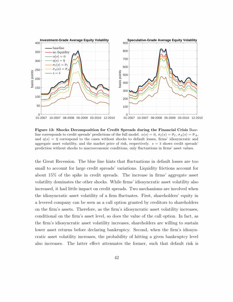
01-2007 10-2007 08-2008 05-2009 03-2010 12-20100
50
100
150
200
250
300
350
400
basi
s po
ints
Investment-Grade Average Equity Volatility
baselineno liquidity,(s) = ,
2(s) = 2
<I(s) = <I
<A(s) = <A
s = s
01-2007 10-2007 08-2008 05-2009 03-2010 12-20100
100
200
300
400
500
600
700
800
900
basi
s po
ints
Speculative-Grade Average Equity Volatility
Figure 13: Shocks Decomposition for Credit Spreads during the Financial Crisis Base-line corresponds to credit spreads’ predictions of the full model. α(s) = α, σI(s) = σI , σA(s) = σA,and η(s) = η correspond to the cases without shocks to default losses, firms’ idiosyncratic andaggregate asset volatility, and the market price of risk, respectively. s = s shows credit spreads’prediction without shocks to macroeconomic conditions, only fluctuations in firms’ asset values.
the Great Recession. The blue line hints that fluctuations in default losses are too
small to account for large credit spreads’ variations. Liquidity frictions account for
about 15% of the spike in credit spreads. The increase in firms’ aggregate asset
volatility dominates the other shocks. While firms’ idiosyncratic asset volatility also
increased, it had little impact on credit spreads. Two mechanisms are involved when
the idiosyncratic asset volatility of a firm fluctuates. First, shareholders’ equity in
a levered company can be seen as a call option granted by creditors to shareholders
on the firm’s assets. Therefore, as the firm’s idiosyncratic asset volatility increases,
conditional on the firm’s asset level, so does the value of the call option. In fact, as
the firm’s idiosyncratic asset volatility increases, shareholders are willing to sustain
lower asset returns before declaring bankruptcy. Second, when the firm’s idiosyn-
cratic asset volatility increases, the probability of hitting a given bankruptcy level
also increases. The latter effect attenuates the former, such that default risk is
42
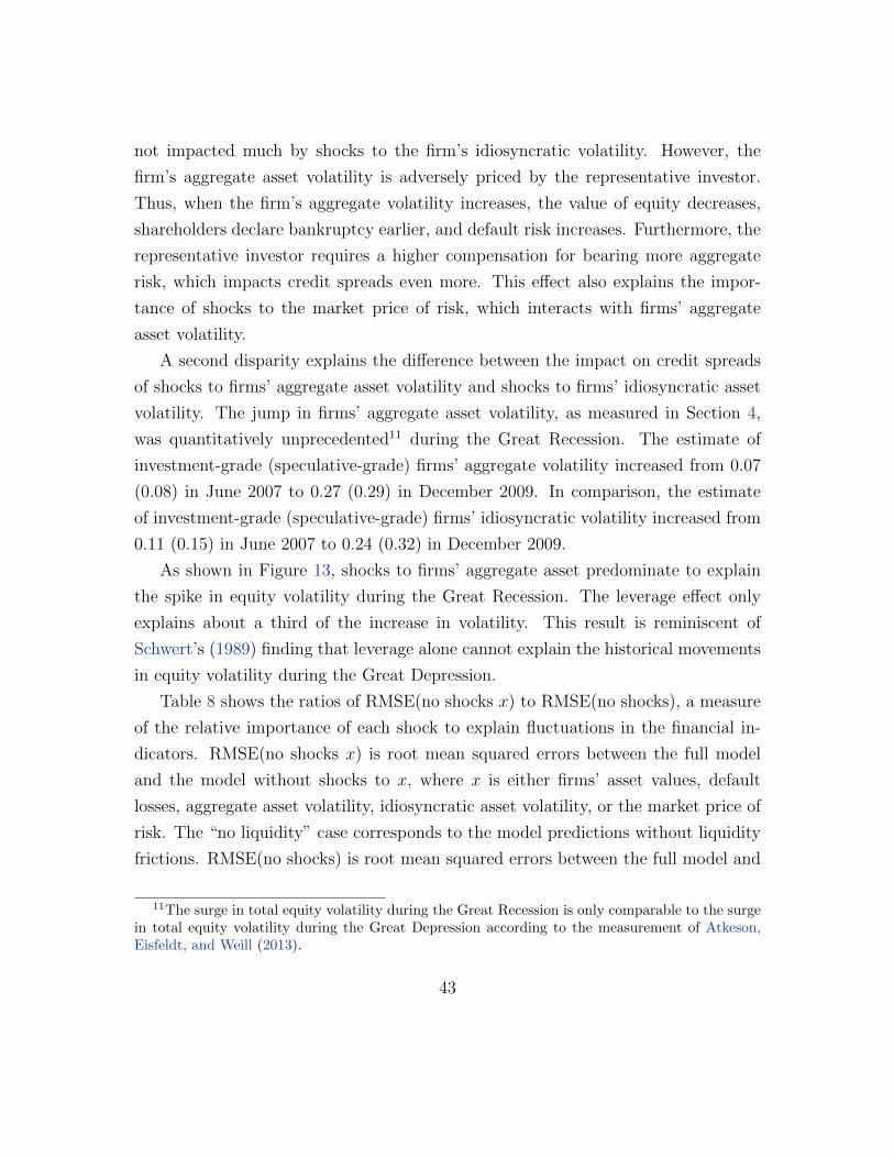
not impacted much by shocks to the firm’s idiosyncratic volatility. However, the
firm’s aggregate asset volatility is adversely priced by the representative investor.
Thus, when the firm’s aggregate volatility increases, the value of equity decreases,
shareholders declare bankruptcy earlier, and default risk increases. Furthermore, the
representative investor requires a higher compensation for bearing more aggregate
risk, which impacts credit spreads even more. This effect also explains the impor-
tance of shocks to the market price of risk, which interacts with firms’ aggregate
asset volatility.
A second disparity explains the difference between the impact on credit spreads
of shocks to firms’ aggregate asset volatility and shocks to firms’ idiosyncratic asset
volatility. The jump in firms’ aggregate asset volatility, as measured in Section 4,
was quantitatively unprecedented11 during the Great Recession. The estimate of
investment-grade (speculative-grade) firms’ aggregate volatility increased from 0.07
(0.08) in June 2007 to 0.27 (0.29) in December 2009. In comparison, the estimate
of investment-grade (speculative-grade) firms’ idiosyncratic volatility increased from
0.11 (0.15) in June 2007 to 0.24 (0.32) in December 2009.
As shown in Figure 13, shocks to firms’ aggregate asset predominate to explain
the spike in equity volatility during the Great Recession. The leverage effect only
explains about a third of the increase in volatility. This result is reminiscent of
Schwert’s (1989) finding that leverage alone cannot explain the historical movements
in equity volatility during the Great Depression.
Table 8 shows the ratios of RMSE(no shocks x) to RMSE(no shocks), a measure
of the relative importance of each shock to explain fluctuations in the financial in-
dicators. RMSE(no shocks x) is root mean squared errors between the full model
and the model without shocks to x, where x is either firms’ asset values, default
losses, aggregate asset volatility, idiosyncratic asset volatility, or the market price of
risk. The “no liquidity” case corresponds to the model predictions without liquidity
frictions. RMSE(no shocks) is root mean squared errors between the full model and
11The surge in total equity volatility during the Great Recession is only comparable to the surgein total equity volatility during the Great Depression according to the measurement of Atkeson,Eisfeldt, and Weill (2013).
43
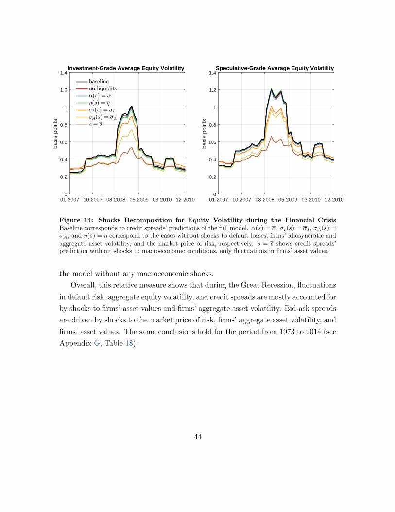
01-2007 10-2007 08-2008 05-2009 03-2010 12-20100
0.2
0.4
0.6
0.8
1
1.2
1.4
basi
s po
ints
Investment-Grade Average Equity Volatility
baselineno liquidity,(s) = ,
2(s) = 2
<I(s) = <I
<A(s) = <A
s = s
01-2007 10-2007 08-2008 05-2009 03-2010 12-20100
0.2
0.4
0.6
0.8
1
1.2
1.4
basi
s po
ints
Speculative-Grade Average Equity Volatility
Figure 14: Shocks Decomposition for Equity Volatility during the Financial CrisisBaseline corresponds to credit spreads’ predictions of the full model. α(s) = α, σI(s) = σI , σA(s) =σA, and η(s) = η correspond to the cases without shocks to default losses, firms’ idiosyncratic andaggregate asset volatility, and the market price of risk, respectively. s = s shows credit spreads’prediction without shocks to macroeconomic conditions, only fluctuations in firms’ asset values.
the model without any macroeconomic shocks.
Overall, this relative measure shows that during the Great Recession, fluctuations
in default risk, aggregate equity volatility, and credit spreads are mostly accounted for
by shocks to firms’ asset values and firms’ aggregate asset volatility. Bid-ask spreads
are driven by shocks to the market price of risk, firms’ aggregate asset volatility, and
firms’ asset values. The same conclusions hold for the period from 1973 to 2014 (see
Appendix G, Table 18).
44
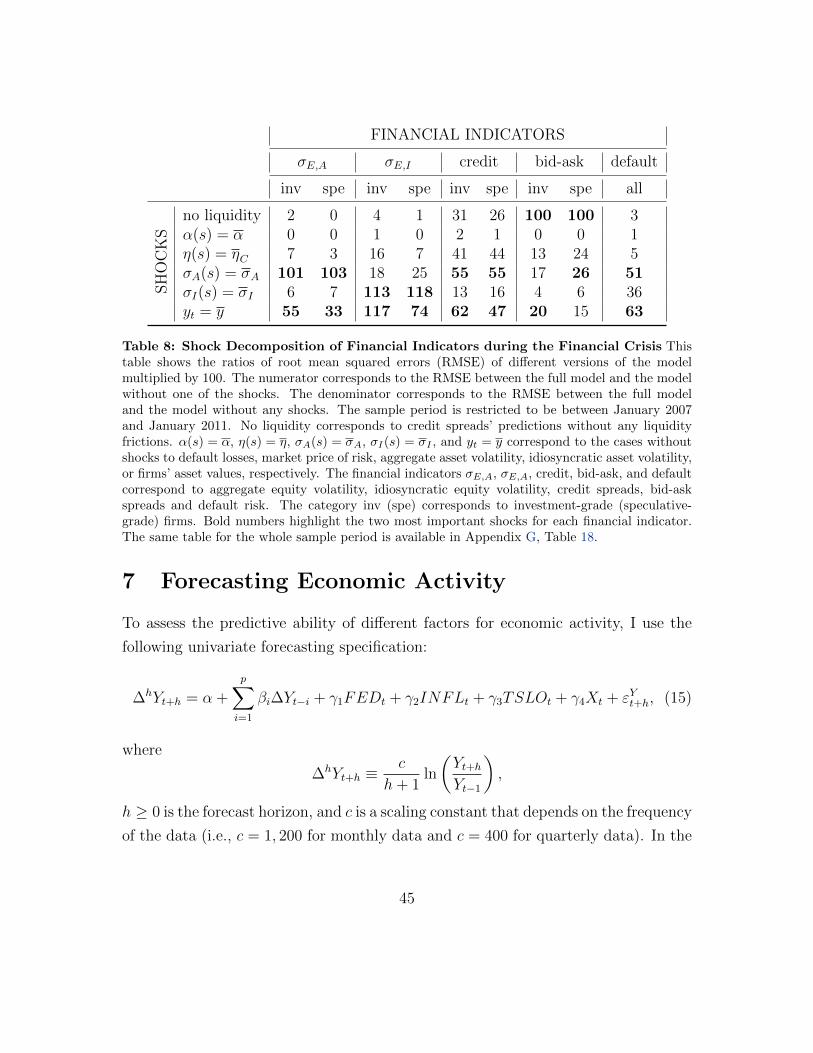
FINANCIAL INDICATORS
σE,A σE,I credit bid-ask default
inv spe inv spe inv spe inv spe all
SH
OC
KS
no liquidity 2 0 4 1 31 26 100 100 3α(s) = α 0 0 1 0 2 1 0 0 1η(s) = ηC 7 3 16 7 41 44 13 24 5σA(s) = σA 101 103 18 25 55 55 17 26 51σI(s) = σI 6 7 113 118 13 16 4 6 36yt = y 55 33 117 74 62 47 20 15 63
Table 8: Shock Decomposition of Financial Indicators during the Financial Crisis Thistable shows the ratios of root mean squared errors (RMSE) of different versions of the modelmultiplied by 100. The numerator corresponds to the RMSE between the full model and the modelwithout one of the shocks. The denominator corresponds to the RMSE between the full modeland the model without any shocks. The sample period is restricted to be between January 2007and January 2011. No liquidity corresponds to credit spreads’ predictions without any liquidityfrictions. α(s) = α, η(s) = η, σA(s) = σA, σI(s) = σI , and yt = y correspond to the cases withoutshocks to default losses, market price of risk, aggregate asset volatility, idiosyncratic asset volatility,or firms’ asset values, respectively. The financial indicators σE,A, σE,A, credit, bid-ask, and defaultcorrespond to aggregate equity volatility, idiosyncratic equity volatility, credit spreads, bid-askspreads and default risk. The category inv (spe) corresponds to investment-grade (speculative-grade) firms. Bold numbers highlight the two most important shocks for each financial indicator.The same table for the whole sample period is available in Appendix G, Table 18.
7 Forecasting Economic Activity
To assess the predictive ability of different factors for economic activity, I use the
following univariate forecasting specification:
∆hYt+h = α +
p∑i=1
βi∆Yt−i + γ1FEDt + γ2INFLt + γ3TSLOt + γ4Xt + εYt+h, (15)
where
∆hYt+h ≡c
h+ 1ln
(Yt+hYt−1
),
h ≥ 0 is the forecast horizon, and c is a scaling constant that depends on the frequency
of the data (i.e., c = 1, 200 for monthly data and c = 400 for quarterly data). In the
45
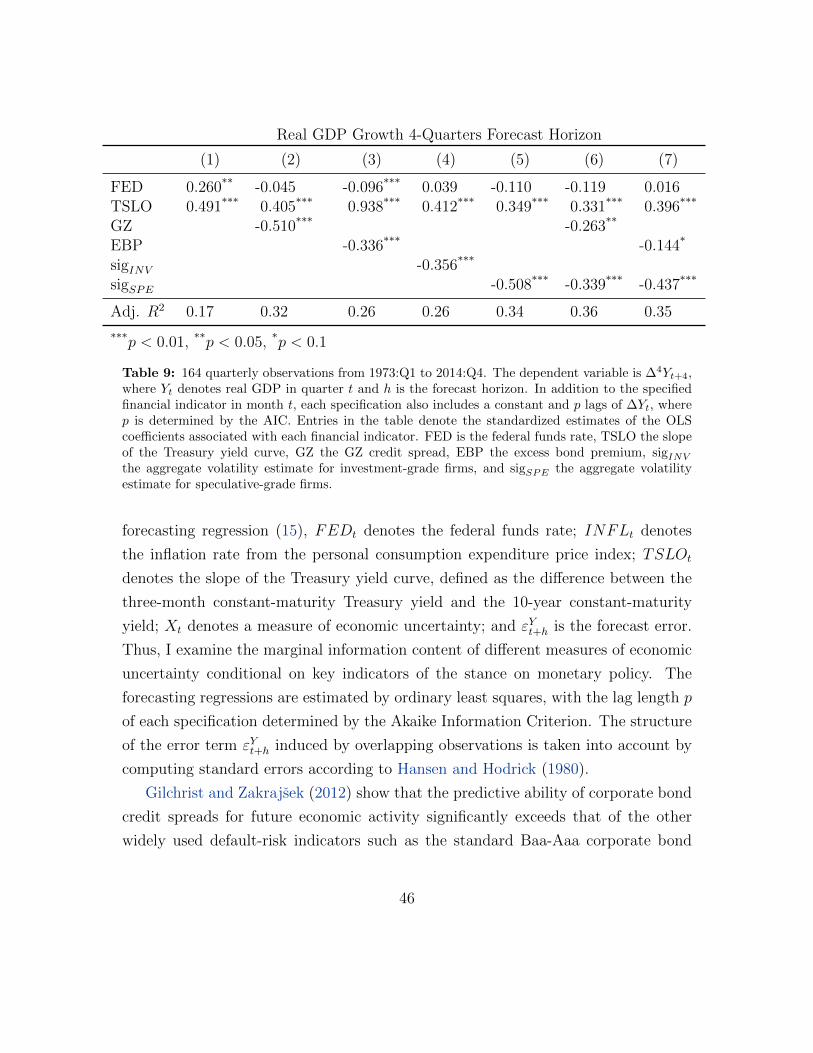
Real GDP Growth 4-Quarters Forecast Horizon
(1) (2) (3) (4) (5) (6) (7)
FED 0.260** -0.045 -0.096*** 0.039 -0.110 -0.119 0.016TSLO 0.491*** 0.405*** 0.938*** 0.412*** 0.349*** 0.331*** 0.396***
GZ -0.510*** -0.263**
EBP -0.336*** -0.144*
sigINV -0.356***
sigSPE -0.508*** -0.339*** -0.437***
Adj. R2 0.17 0.32 0.26 0.26 0.34 0.36 0.35
***p < 0.01, **p < 0.05, *p < 0.1
Table 9: 164 quarterly observations from 1973:Q1 to 2014:Q4. The dependent variable is ∆4Yt+4,where Yt denotes real GDP in quarter t and h is the forecast horizon. In addition to the specifiedfinancial indicator in month t, each specification also includes a constant and p lags of ∆Yt, wherep is determined by the AIC. Entries in the table denote the standardized estimates of the OLScoefficients associated with each financial indicator. FED is the federal funds rate, TSLO the slopeof the Treasury yield curve, GZ the GZ credit spread, EBP the excess bond premium, sigINVthe aggregate volatility estimate for investment-grade firms, and sigSPE the aggregate volatilityestimate for speculative-grade firms.
forecasting regression (15), FEDt denotes the federal funds rate; INFLt denotes
the inflation rate from the personal consumption expenditure price index; TSLOt
denotes the slope of the Treasury yield curve, defined as the difference between the
three-month constant-maturity Treasury yield and the 10-year constant-maturity
yield; Xt denotes a measure of economic uncertainty; and εYt+h is the forecast error.
Thus, I examine the marginal information content of different measures of economic
uncertainty conditional on key indicators of the stance on monetary policy. The
forecasting regressions are estimated by ordinary least squares, with the lag length p
of each specification determined by the Akaike Information Criterion. The structure
of the error term εYt+h induced by overlapping observations is taken into account by
computing standard errors according to Hansen and Hodrick (1980).
Gilchrist and Zakrajsek (2012) show that the predictive ability of corporate bond
credit spreads for future economic activity significantly exceeds that of the other
widely used default-risk indicators such as the standard Baa-Aaa corporate bond
46
credit spread and the paper-bill spread. Therefore, I compare the performance of
firms’ aggregate asset volatility with the GZ credit spread, which is the monthly aver-
age of corporate bond credit spreads, and the excess bond premium, which captures
the cyclical changes in the relationship between measured default risk and credit
spreads (see Gilchrist and Zakrajsek, 2012, for details).
A model-free approximation to the estimated aggregate volatility time series from
Section 4 is given by:
log(sigjt)
=1
Njt
∑i∈I(j,t)
[log(1− levit) + log
(viE,A(t)
)],
where Njt is the amount of firms of type j at time t and I(j, t) is the set of firms of
type j at time t. Market leverage levit and equity return aggregate volatility viE,A(t)
are described in Section 3. This approximation is more convenient to construct from
a panel dataset of equity and leverage, captures accurately the levels and fluctua-
tions in the estimated aggregate asset volatility, and does not significantly alter the
forecasting results. Derivation of this approximation is provided in Appendix F.
Thus, recovering an accurate measure of aggregate asset volatility does not depend
on departures from Modigliani and Miller’s (1958) assumptions. This provides an
important guidance for future research. The predictions of a mechanism that relates
fluctuations in aggregate asset volatility to future economic activity should satisfy
this regularity.
The second and third columns of Table 9 replicate the forecasting regressions
of Gilchrist and Zakrajsek (2012) for the GZ credit spread and the excess bond
premium, which have considerable predictive power for economic activity over the
1973–2014 period.
As indicated in the fourth and fifth columns of Table 9, firms’ aggregate asset
volatility is both economically and statistically a highly significant predictor of out-
put growth at the year-ahead forecast horizon over the full sample period. Firms’
aggregate asset volatility of speculative-grade firms is economically a stronger pre-
dictor of output growth than firms’ aggregate asset volatility of investment-grade
47
firms. The coefficient estimate implies that an increase in the investment-grade
(speculative-grade) firms’ aggregate asset volatility of 10 volatility points in quarter
t leads to a drop in real GDP growth of more than 2 (2.5) percentage points over
the subsequent 4 quarters.
The sixth and seventh columns show that the GZ credit spread and the excess
bond premium do not contain significant independent explanatory power on top of
firms’ aggregate asset volatility to predict output growth. In other words, the in-
formational content of corporate bond credit spreads for predicting output growth
is captured by fluctuations in firms’ aggregate asset volatility. For completeness, I
replicated the forecast regressions of Gilchrist and Zakrajsek (2012) with payroll em-
ployment, unemployment rate, and industrial production at 3- and 12-month forecast
horizons. Overall, firms’ aggregate asset volatility does not outperform the GZ credit
spread for these components but captures at least 60% of the credit spreads’ fore-
casting power for all of these indicators of real economic activity.12 Aggregate asset
volatility significantly outperforms aggregate equity volatility to predict economic
activity.
8 Conclusion
In this paper, I show that a structural model estimated with a large firm-level
database can successfully account for the joint dynamics of important financial indi-
cators of uncertainty and financial distress. I uncover that fluctuations in firms’ asset
values and firms’ aggregate asset volatility are the main drivers of these financial in-
dicators. According to the structure of the model, it occurs because firms’ aggregate
12The percentage of credit spreads’ forecasting power captured by aggregate volatility is definedas:
R2SIG −R2
0
R2GZ −R2
0
.
R2SIG is the adjusted goodness of fit of a regression with FED and TSLO. R2
SIG is the adjustedgoodness of fit of a regression with FED, TSLO, and sigINV or sigSPE . R2
GZ is the adjustedgoodness of fit of a regression with FED, TSLO, and GZ.
48

volatility greatly influences the quantity of credit risk priced by the representative
investor. Furthermore, the informational content of these financial indicators for
predicting real economic activity can be captured by fluctuations in firms’ aggre-
gate asset volatility. All together, my results suggest that fluctuations in aggregate
firms’ asset volatility are key for the transmission channel that links the fundamen-
tal drivers of financial indicators to the real economy. Further research should aim
at understanding the links between fundamental shocks, financial indicators, and
macroeconomic aggregates in a general equilibrium framework.
References
Almeida, Heitor and Philippon, Thomas. The risk-adjusted cost of financial distress.
The Journal of Finance, 62(6):2557–2586, 2007.
Atkeson, Andrew, Eisfeldt, Andrea, and Weill, Pierre-Olivier. Measuring the finan-
cial soundness of us firms, 1926-2012. Technical report, National Bureau of Economic
Research, 2013.
Bansal, Ravi and Yaron, Amir. Risks for the long run: A potential resolution of
asset pricing puzzles. The Journal of Finance, 59(4):1481–1509, 2004.
Bao, Jack, Pan, Jun, and Wang, Jiang. The illiquidity of corporate bonds. The
Journal of Finance, 66(3):911–946, 2011.
Bhamra, Harjoat, Kuehn, Lars-Alexander, and Strebulaev, Ilya. The levered equity
risk premium and credit spreads: A unified framework. Review of Financial Studies,
23(2):645–703, 2010.
Bloom, Nicholas. The impact of uncertainty shocks. Econometrica, 77(3):623–685,
2009.
Caldara, Dario, Fuentes-Albero, Cristina, Gilchrist, Simon, and Zakrajsek, Egon.
The macroeconomic impact of financial and uncertainty shocks. European Economic
Review, 2016.
49

Carhart, Mark. On persistence in mutual fund performance. The Journal of finance,
52(1):57–82, 1997.
Chen, Hui. Macroeconomic conditions and the puzzles of credit spreads and capital
structure. The Journal of Finance, 65(6):2171–2212, 2010.
Chen, Hui, Cui, Rui, He, Zhiguo, and Milbradt, Konstantin. Quantifying liquidity
and default risks of corporate bonds over the business cycle. Technical report, 2016.
Working paper.
Chen, Long, Collin-Dufresne, Pierre, and Goldstein, Robert. On the relation between
the credit spread puzzle and the equity premium puzzle. Review of Financial Studies,
22(9):3367–3409, 2009.
Collin-Dufresne, Pierre, Goldstein, Robert, and Martin, Spencer. The determinants
of credit spread changes. The Journal of Finance, 56(6):2177–2207, 2001.
David, Alexander. Inflation uncertainty, asset valuations, and the credit spreads
puzzle. Review of Financial Studies, 21(6):2487–2534, 2008.
Duffee, Gregory R. Estimating the price of default risk. Review of Financial Studies,
12(1):197–226, 1999.
Duffie, Darrell and Epstein, Larry. Stochastic differential utility. Econometrica:
Journal of the Econometric Society, pages 353–394, 1992.
Duffie, Darrell and Singleton, Kenneth J. An econometric model of the term structure
of interest-rate swap yields. The Journal of Finance, 52(4):1287–1321, 1997.
Duffie, Darrell, Garleanu, Nicolae, and Pedersen, Lasse Heje. Over-the-counter mar-
kets. Econometrica, 73(6):1815–1847, 2005.
Edwards, Amy, Harris, Lawrence, and Piwowar, Michael. Corporate bond market
transaction costs and transparency. The Journal of Finance, 62(3):1421–1451, 2007.
50

Elton, Edwin J, Gruber, Martin J, Agrawal, Deepak, and Mann, Christopher. Ex-
plaining the rate spread on corporate bonds. The Journal of Finance, 56(1):247–277,
2001.
Epstein, Larry and Zin, Stanley. Substitution, risk aversion, and the temporal be-
havior of consumption and asset returns: A theoretical framework. Econometrica:
Journal of the Econometric Society, pages 937–969, 1989.
Estrella, Arturo and Hardouvelis, Gikas. The term structure as a predictor of real
economic activity. The Journal of Finance, 46(2):555–576, 1991.
Fama, Eugene and French, Kenneth. The cross-section of expected stock returns.
the Journal of Finance, 47(2):427–465, 1992.
Faust, Jon, Gilchrist, Simon, Wright, Jonathan, and Zakrajsek, Egon. Credit spreads
as predictors of real-time economic activity: a bayesian model-averaging approach.
Review of Economics and Statistics, 95(5):1501–1519, 2013.
Feldhutter, Peter. The same bond at different prices: identifying search frictions and
selling pressures. Review of Financial Studies, 25(4):1155–1206, 2012.
Friedman, Benjamin and Kuttner, Kenneth. Another look at the evidence on money-
income causality. Journal of Econometrics, 57(1-3):189–203, 1993.
Gertler, Mark and Lown, Cara. The information in the high-yield bond spread for
the business cycle: evidence and some implications. Oxford Review of Economic
Policy, 15(3):132–150, 1999.
Gilchrist, Simon and Zakrajsek, Egon. Credit spreads and business cycle fluctuations.
The American Economic Review, 102(4):1692–1720, 2012.
Gilchrist, Simon, Yankov, Vladimir, and Zakrajsek, Egon. Credit market shocks and
economic fluctuations: Evidence from corporate bond and stock markets. Journal of
monetary Economics, 56(4):471–493, 2009.
51
Graham, John. How big are the tax benefits of debt? The Journal of Finance, 55
(5):1901–1941, 2000.
Hackbarth, Dirk, Miao, Jianjun, and Morellec, Erwan. Capital structure, credit
risk, and macroeconomic conditions. Journal of Financial Economics, 82(3):519–
550, 2006.
Hansen, Lars Peter and Hodrick, Robert. Forward exchange rates as optimal predic-
tors of future spot rates: An econometric analysis. The Journal of Political Economy,
pages 829–853, 1980.
Harvey, Campbell. The real term structure and consumption growth. Journal of
Financial Economics, 22(2):305–333, 1988.
He, Zhiguo and Milbradt, Konstantin. Endogenous liquidity and defaultable bonds.
Econometrica, 82(4):1443–1508, 2014.
Herskovic, Bernard, Kelly, Bryan, Lustig, Hanno, and Van Nieuwerburgh, Stijn. The
common factor in idiosyncratic volatility: Quantitative asset pricing implications.
Journal of Financial Economics, 119(2):249–283, 2016.
Huang, Jing-Zhi and Huang, Ming. How much of the corporate-treasury yield spread
is due to credit risk? Review of Asset Pricing Studies, 2(2):153–202, 2012.
King, Thomas, Levin, Andrew, and Perli, Roberto. Financial market perceptions of
recession risk. 2007.
Leland, Hayne E. Corporate debt value, bond covenants, and optimal capital struc-
ture. The journal of finance, 49(4):1213–1252, 1994.
Longstaff, Francis, Mithal, Sanjay, and Neis, Eric. Corporate yield spreads: Default
risk or liquidity? new evidence from the credit default swap market. The Journal of
Finance, 60(5):2213–2253, 2005.
Modigliani, Franco and Miller, Merton. The cost of capital, corporation finance and
the theory of investment. The American economic review, pages 261–297, 1958.
52
Mody, Ashoka and Taylor, Mark. Financial predictors of real activity and the finan-
cial accelerator. Economics Letters, 82(2):167–172, 2004.
Philippon, Thomas. The bond market’s q. The Quarterly Journal of Economics, 124
(3):1011–1056, 2009.
Rajan, Raghuram and Zingales, Luigi. What do we know about capital structure?
some evidence from international data. The journal of Finance, 50(5):1421–1460,
1995.
Roll, Richard. A simple implicit measure of the effective bid-ask spread in an efficient
market. The Journal of Finance, 39(4):1127–1139, 1984.
Schwert, William. Why does stock market volatility change over time? The journal
of finance, 44(5):1115–1153, 1989.
Shleifer, Andrei and Vishny, Robert. Liquidation values and debt capacity: A market
equilibrium approach. The Journal of Finance, 47(4):1343–1366, 1992.
Stock, James and Watson, Mark. Disentangling the channels of the 2007-2009 reces-
sion. Technical report, National Bureau of Economic Research, 2012.
Strebulaev, Ilya and Yang, Baozhong. The mystery of zero-leverage firms. Journal
of Financial Economics, 109(1):1–23, 2013.
Tauchen, George. Finite state markov-chain approximations to univariate and vector
autoregressions. Economics letters, 20(2):177–181, 1986.
53

Appendices
A The Marginal Investor Stochastic Discount Fac-
tor
To obtain the stochastic discount factor, I first solve for the value function of the
representative household as
J(Ct, st) = Et[∫ ∞
0
f(Ct+s, Jt+s)ds
],
where the function f(c, v) is a normalized aggregator of consumption and continua-
tion value in each period defined as
f(C, J) =ρ
1− 1/ψ
C1−1/ψ − ((1− γ)J)1−1/ψ1−γ
((1− γ)J)1−1/ψ1−γ −1
.
The consumption process of the marginal investor follows:
dCtCt
= µCdt+ σC(s)dZAt .
The Hamilton-Jacoby-Bellman equation in state s (for s = 1, . . . , S) is
0 = f(C, J(C, s)) + JC(C, s)CµC +1
2JCC(C, s)C2σ2
C(s) +∑s′ 6=s
ζPss′(J(C, s′)− J(C, s)).
Conjecture that the solution for J is
J(C, s) =(h(s)C)1−γ
1− γ.
54

Note that
JC(C, s) = (h(s)C)−γ ,
JCC(C, s) = −γ (h(s)C)−γ−1 .
Substituting J into the differential equations above, we get the following system of
nonlinear equations for h:
0 =ρ
1− 1/ψ
(h(s)1/ψ−γ − h(s)1−γ
)C1−γ + h(s)−γC1−γµC −
1
2γ (h(s)C)1−γ σ2
C(s)
+∑s′ 6=s
ζPss′
((h(s′)C)1−γ
1− γ− (h(s)C)1−γ
1− γ
).
This can be simplified as
0 = ρ1− γ
1− 1/ψh(s)1/ψ−γ +
[(1− γ)µC −
1
2γ(1− γ)σ2
C(s)− ρ 1− γ1− 1/ψ
]h(s)1−γ
+∑s′ 6=s
ζPss′(h(s′)1−γ − h(s)1−γ
).
While no algebraic solution exists for this system of nonlinear equations, it is trivial
to solve numerically for h(s) ∀s ∈ 1, . . . , S. Duffie and Skiadas (1994) show that
the stochastic discount factor is equal to
Λt = exp
(∫ t
0
fJ(Cu, Ju)du
)fC(Ct, Jt).
Thus we have
Λt = exp
(∫ t
0
ρ(1− γ)
1− 1/ψ
((1/ψ − γ
1− γ
)h(su)
1/ψ−1 − 1
)du
)ρH(s)1/ψ−γC−γ.
55

Applying Ito’s formula with jumps, we get
dΛt
Λt
= −r(s)dt− η(s)dZMt +
∑s′ 6=s
(eκ(s,s
′) − 1)dM s,s′
t ,
where
r(s) = −ρ(1− γ)
1− 1/ψ
[1/ψ − γ
1− γh(s)1/ψ−1 − 1
]+ γµC(s)− 1
2γ(1 + γ)σ2
C(s)−∑s′ 6=s
(eκ(s,s′) − 1)
η(s) = γσC(s)
κ(s, s′) = (1/ψ − γ) log
(h(j)
h(i)
).
56
B Solution to Bond and Equity Valuation
The solution method presented in this appendix is based on Chen, Cui, He, and
Milbradt (2016).
Notation for Matrix Formulation I follow the Markov-modulated dynamics
approach of Jobert and Rogers (2006). Define y to be the log of the level of cash
flows given by:
dy = µsdt+ σsdZt
where Zt is a Brownian motion. The firm go bankrupt if y becomes lower than
given bankruptcy boundaries in each state. There are multiple possible bankruptcy
boundaries, ybs , for each aggregate state s. Order states s such that s > s′ implies
that ybs > ybs′ and denote the intervals Is = [ybs, ybs+1] where ybS+1 = ∞, so that
Is ∩ Is+1 = ybs+1. Let yb = [yb1, ..., ybs]T be the vector of bankruptcy boundaries.
Let’s use the following notation for the solution of debt functions within each interval:
Djs,i ≡ Dj
s(y), y ∈ Ii, that is Djs,i is the restriction of Dj
s(y) to the interval Ii. Thus,
Djs,i = recovery value for any i < s, as it would imply that the company immediately
defaults in interval Ii for state s. Let’s stack the alive functions along states s but
still restricted to interval i so that Di = [DH1,i, D
L1,i, D
H2,i, D
L2,i, . . . , D
Hi,i, D
Li,i]
T. Let Ii
be the i-dimensional identity matrix, and let be 1i a column vector of ones of length
i. Let’s define matrices of parameters:
Ri =
r1 +m+ ϕ+ ζ1 0 · · · −ζ1,i 0
0 r1 +m+ ϕ+ ζ1 · · · 0 −ζ1,i...
.... . .
......
−ζi,1 0 · · · ri +m+ ϕ+ ζi 0
0 −ζi,1 · · · 0 ri +m+ ϕ+ ζi
,
57
where ζs =∑
s′ 6=s ζs,s′
Qi =
ξH1 −ξH1 · · · 0 0
−ξL1 − χ1(1 + β)/2 ξL1 − χ1(1− β)/2 · · · 0 0...
.... . .
......
0 0 · · · ξHi −ξHi0 0 · · · −ξLi − χiwH ξLi − χiwL
,
Gi =
ζ1,i+1 0 · · · ζ1,S 0
0 ζ1,i+1 · · · 0 ζ1,S...
.... . .
......
ζi,i+1 0 · · · ζi,S 0
0 ζi,i+1 · · · 0 ζi,S
, bi =
αHi+1vi+1
αHi+1vi+1
...
αHS vS
αLSvS
,
v =
v1...
vS
=
r1 − µ1 + ζ1 −ζ1,2 · · · −ζ1,i−ζ2,1 r2 − µ2 + ζ2 · · · −ζ2,i
......
. . ....
−ζi,1 −ζi,2 · · · ri − µi + ζi
−1
1S,
Ni = [0, N, · · · , 0, N ]T, χi = diag ([χ1, χ1, · · · , χi, χi]), Σi = diag ([σ21, σ
21, · · · , σ2
i , σ2i ]),
and µi = diag ([µ1, µ1, · · · , µi, µi]).
B.1 Debt Value
Debt valuation follows the following differential equation on interval Ii:
(Ri + Qi)Di(y) = µiD′i(y) + 0.5ΣiD
′′i (y) + (c+mp+ ϕp)12i − χiNi + 1i < SGibi exp(y)
where GiVi exp(y) represents the intensity of jumping into default times the recovery
in the default state. We can rewrite the problem as a linear system of differential
58
equations as
x′(y) =
[D′′i (y)
D′i(y)
]=
[−2Σ−1i µi 2Σ−1i (Ri + Qi)
I2i 02i
][D′i(y)
Di(y)
]+ fi(y) = Aixi(y) + fi(y)
where
fi(y) =
[−(c+mp+ ϕp)2Σ−1i 12i + 2Σ−1i χiNi − 1i < S2Σ−1i Gibi exp(y)
02i
].
We know that the general solution xi(y) is given by the expression
xi(y) = xhi (y) + xpi (y).
The term xhi (y) is the general solution of the homogeneous equation x′i(y) = Aixi(y)
in which are to be found 4i arbitrary constants c1, . . . , c4i. The term xpi (y) is a
particular solution of x′i(y) = Axi(y) + fi(y). The general solution of the linear
system x′i(y) = Axi(y) is given by
xi(y) = c1ih1i eλ1i y + . . .+ c4ii h4i
i eλ4ii y = HiΛi(y)ci.
where (λ1i ,h1i ), . . ., (λ4ii ,h
4ii ) are the eigenpairs of Ai with 4i independent eigenvec-
tors, and
Hi = [h1i , . . . ,h
4ii ],
ci = [c1i , . . . , c4ii ]T,
Λi(y) = diag([eλ
1i y, . . . , eλ
4ii y]).
We can guess a solution of the kind k0i +k1
i exp(y) for the particular solution xpi[1:2i](y)
where x[1:2i] selects the first 2i rows of vector x. Therefore, we can solve for the
59
coefficients by substituting in:
(Ri + Qi)(k0i + k1
i exp(y))
= µik1i exp(y) + 0.5Σik
1i exp(y)
+ (c+mp+ ϕp)12i − χiNi + 1i < SGibi exp(y),
and solve for any value of y. This gives us
k0i = (Ri + Qi)
−1 ((c+mp+ ϕp)12i − χiNi) ,
k1i = (Ri + Qi − µi − 0.5Σi)
−1 1i < SGibi.
Thus we have
Di(y) = HiΛi(y)ci + k0i + k1
i exp(y)
where Hi = Hi[1:2i] and X[1:2i] selects the first 2i rows of matrix X, and
D′i(y) = HiλiΛi(y)ci + k1i exp(y).
where
λi = diag([λ1i , . . . , λ
4ii
]).
Boundary Conditions The different value functions Di for i ∈ 1, . . . , S are
linked at the boundaries of their domains Ii. Note that Ii ∩ Ii+1 = ybi+1 for i < S.
For i = S , we can immediately rule out all positive solutions to λi as debt has to
be finite and bounded as y →∞, so that the entries of ci corresponding to positive
eigenvalues will be zero:
limy→∞|DS(y)| <∞.
For i < S, we must have value matching of the value functions that are alive across
the boundary, and we must have value matching of the value functions that die across
60

the boundary:
Di+1(ybi+1) =
[Di(ybi+1)
di+1 exp(ybi+1)
],
where
di+1 =
[αHi+1vi+1
αLi+1vi+1
].
For i < S, we must have smooth pasting of the value functions that are alive across
the boundary:
D′i+1(ybi+1)[1:2i] = D′i(ybi+1)
where x[1:2i] selects the first 2i rows of vector x. Lastly, for i = 1, we must have
D1(yb1) = d1 exp(yb1).
Therefore, given yb the system of 2S2 +2S equations to solve for ci ∀i ∈ 1, . . . , S
can be given by
Hi[2i−1:2i]Λi(ybi)ci + k0i[2i−1:2i] + k1
i[2i−1:2i] exp(ybi) = di exp(ybi) for i = 1, . . . , S
Hi[1:2i−2]Λi(ybi)ci + k0i[1:2i−2] + k1
i+1[1:2i−2] exp(ybi) = Hi−1Λi−1(ybi)ci−1 + k0i−1 + k1
i−1 exp(ybi)
Hi[1:2i−2]λiΛi(ybi)ci + k1i[1:2i−2] exp(ybi) = Hi−1λi−1Λi−1(ybi)ci−1 + k1
i−1 exp(ybi)
for i = 2, . . . , S, and
limy→∞|DS(y)| <∞.
61

We can define squared matrices Mi, Mi, Mi, Ki, Ki , and sKi as
Mi(y) =
[HiΛi(y)
HiλiΛi(y)
], Ki(y) =
[k0i + k1
i exp(y)
k1i exp(y)
],
Mi(y) =
[Hi[1:2i−2]Λi(y)
Hi[1:2i−2]λiΛi(y)
], Ki(y) =
[k0i[1:2i−2] + k1
i[1:2i−2] exp(y)
k1i[1:2i−2] exp(y)
],
Mi(y) = Hi[2i−1:2i]Λi(y), sKi(y) = k0i[2i−1:2i] + k1
i[1:2i−2] exp(y).
With this notation, we can express ci as a linear system of ci+1 with the smooth
pasting conditions:
ci = Mi(ybi+1)−1Mi+1(ybi+1)ci+1 + Mi(ybi+1)
−1(Ki+1(ybi+1)−Ki(ybi+1)
).
Going forward, we can express ci as a linear system of cS:
ci = MMicS + KKi,
where
MMi =
(S−1∏j=i
Mj(ybj+1)−1Mj+1(ybj+1)
),
KKi =S−1∑k=i
(k−1∏j=i
Mj(ybj+1)−1Mj+1(ybj+1)
)Mk(ybk+1)
−1(Kk+1(ybk+1)−Kk(ybk+1)
).
The default boundary conditions can then be expressed as a linear system of cS:
Mi(ybi)MMicS = di exp(ybi)−Mi(ybi)KKi − sKi(ybi).
Stacking all the default boundary conditions, we obtain a squared matrix which
62

can be inversed:
cS =
M1(yb1)MM1
...MS−1(ybS−1)MMS−1
MS(ybS)
LS
−1
d1 exp(yb1)−M1(yb1)KK1 − sK1(yb1)...
dS−1 exp(ybS−1)−MS−1(ybS−1)KKS−1 − sKS−1(ybS−1)
dS exp(ybS)− sKS(ybS)
02S×1
,
where LS is a 2S × 4S matrix such that LcS is the 2S × 1 row vector of ckS such
that λkS > 0. Therefore, given yb, solving for bond valuations resorts to solve for
2S2 − 2S eigenpairs and inverse a 4S × 4S matrix.
Example with 2 States, No Search/Liquidity Frictions, and No Restruc-
turation The first second order differential to be satisfied is given by:
(r1 +m+ ζ1)D1(y) = µ1D′1(y) + 0.5σ2
1D′′1(y) + (c+mp) + ζ1α2v2 exp(y).
The solution will be of the form:
D1(y) = c11eλ11y + c21e
λ21y + k01 + k11 exp(y).
We can solve for the eigenvalues as
A1 =
[−2σ−21 µ1 2σ−21 (r1 +m+ ζ1)
1 0
],
det
([−2σ−21 µ1 − λ 2σ−21 (r1 +m+ ζ1)
1 −λ
])= λ2 + 2σ−21 µ1λ− 2σ−21 (r1 +m+ ζ1),
λ1,21 =−µ1 ±
√µ21 + 2σ2
1(r1 +m+ ζ1)
σ21
.
63

The constant terms k01 and k11 need to satisfy
(r1 +m+ ζ1)(k01 + k11 exp(y)
)= µ1k
11 exp(y) + 0.5σ2
1k11 exp(y) + (c+mp) + ζ1α2v2 exp(y).
Therefore,
k01 =c+mp
r1 +m+ ζ1,
k11 =ζ1α2v2
r1 +m+ ζ1 − µ1 − 0.5σ21
.
The second differential to be satisfied is given by:[r1 +m+ ζ1 −ζ1−ζ2 r2 +m+ ζ2
]D2(y) =
[µ1 0
0 µ2
]D′2(y) + 0.5
[σ21 0
0 σ22
]D′′2(y) +
[c+mp
c+mp
].
The solution will be of the form:
D2(y) = c12h2[1:2]eλ12y + c22h2[1:2]e
λ22y + k02,
where we already discarded the general solutions with positive eigenvalues. We have
to solve for the eigenvalues of
A2 =
−2σ−21 µ1 0 2σ−21 (r1 +m+ ζ1) −σ−21 ζ1
0 −2σ−22 µ2 −σ−22 ζ2 2σ−22 (r2 +m+ ζ2)
1 0 0 0
0 1 0 0
.
The presence of ζi’s make the analytical solution to this problem not feasible to write
in this document. The constant terms k01 and k11 need to satisfy
k02 =
[r1 +m+ ζ1 −ζ1−ζ2 r2 +m+ ζ2
]−1 [c+mp
c+mp
].
64

B.2 Equity Value
With regime switching, debt rollover, and restructuration, the equity valuation Es(·)in state s ∈ 1, . . . , S and log cash flows y must satisfy
rsEs(y) = µsE′s(y) + 0.5σsE
′′s (y) + exp(y)− (1− τ)c+m(Ds(y)− p)
+∑i 6=s
ζs,i(Ei(y)− Es(y)) + ϕ((1− w)Fs(y)− p− Es(y)),
where c is the coupon, m the debt rollover rate, τ the tax benefits of debt, ζs,i the
transition intensity from state s to state i, ϕ the arrival intensity of a restructuration
event, and w the issuance cost. Fs(·) is the value of the new firm after debt re-
structuration. In matrix form, and using the same interval notation as for the bond
valuation, we have:
RiEi(y) = µiE′i(y) + 0.5ΣiE
′′i (y) + (exp(y)− (1− τ)c) 1i
+m (SiDi(y)− p1i) + ϕ((1− w)Fi(y)− p1i).
Matrices specific to solving the equity valuations will be written with a hat. We
define the following matrices of parameters:
Ri =
r1 + ζ1 + ϕ · · · −ζ1,i
.... . .
...
−ζi,1 · · · ri + ζi + ϕ
,
Si =
1 0 0 0 · · · 0 0
0 0 1 0 · · · 0 0...
......
.... . .
......
0 0 0 0 · · · 1 0
0 0 0 0 · · · 0 0
,
65
and Σi = diag ([σ21, · · · , σ2
i ]), µi = diag ([µ1, · · · , µi]). Si is a i × 2i matrix that
selects which debt values the firm is able to issue. We can rewrite the problem as a
linear system of differential equations as
x′(y) =
[E′′i (y)
E′i(y)
]=
[−2Σ−1i µi 2Σ−1i Ri
Ii 0i
][E′i(y)
Ei(y)
]+ fi(y) = Aixi(y) + fi(y)
where
fi(y) =
[− (exp(y)− (1− τ)c) 1i −m (SiDi(y)− p1i)− ϕ((1− w)Fi(y)− p1i)
0i
].
We know that the general solution xi(y) is given by the expression
xi(y) = xhi (y) + xpi (y).
The term xhi (y) is the general solution of the homogeneous equation x′i(y) = Aixi(y)
and xpi (y) is a particular solution. The general solution of the linear system x′i(y) =
Axi(y) is given by
xi(y) = c1i h1i eλ1i y + . . .+ c2ii h2i
i eλ2ii y = HiΛi(y)ci.
where (λ1i , h1i ), . . ., (λ2ii , h
2ii ) are the eigenpairs of Ai with 2i independent eigenvec-
tors, and
Hi = [h1i , . . . , h
2ii ],
ci = [c1i , . . . , c2ii ]T,
Λi(y) = diag([eλ
1i y1 , . . . , e
λ2ii y1
]).
I can guess a solution of the kind k0i + k1
i exp(y) for the particular solution xpi[1:i](y)
where x[1:i] selects the first i rows of vector x generated by the constants and the
term in exp(y). Therefore, we can solve for the coefficients by substituting in and
66

using the particular solution of Di(y) and Fi(y):
Ri
(k0i + k1
i exp(y))
= µik1i exp(y) + 0.5Σik
1i exp(y) + (exp(y)− (1− τ)c) 1i
+m(Sik
0i + Sik
1i exp(y)− p1i
)+ ϕ((1− w)fi exp(y)− p1i),
and solve for any value of y. Note that I assumed that the value of the firm after
restructuration has the form fi exp(y). I will prove this later on. This gives us
k0i = R−1i
(−(1− τ)c1i +mSik
0i −mp1i
),
k1i =
(Ri − µi − 0.5Σi
)−1 (1i +mSik
1i + ϕ(1− w)fi
).
For the particular part stemming from the general solution of Di(y) = HiΛi(y)ci,
we can conjecture of non-constant part of the form GiΛi(y)ci which has to satisfy
RiGiΛi(y)ci =(µiGiλi + 0.5ΣiGiλ
2i +mSiHi
)Λi(y)ci
for any value of y. Therefore, the following systems have to hold
RiGi[:,j] = µiGi[:,j]λji + 0.5ΣiGi[:,j](λ
ji )
2 +mSiHi[:,j]
for all j, where Xi[:,j] selects the jth column of matrix Xi and Xi[k,j] selects the scalar
in the kth row jth column of matrix Xi. Solving for Gi[:,j], we have
Gi[:,j] =(Ri − µiλ
ji − 0.5Σi(λ
ji )
2)−1
mSiHi[:,j].
Finally, the general solution is given by
Ei(y) =HiΛi(y)ci + GiΛi(y)ci + k0
i + k1i exp(y)
67

whereHi = Hi[1:i] and X[1:i] selects the first 2i rows of matrix X, and
E′i(y) =HiλiΛi(y)ci + GiλiΛi(y)ci + k1
i exp(y)
where
λi = diag([λ1i , . . . , λ
2ii
]).
Boundary Conditions The different value functions Ei for i ∈ 1, . . . , S are
linked at the boundaries of their domains Ii. Note that Ii ∩ Ii+1 = ybi+1 for i < S.
For i = S , we can immediately rule out all solutions to λi bigger than 1 as equity
over cash flow has to be finite and bounded as y → ∞, so that the entries of ci
corresponding to eigenvalues larger than 1 will be zero:
limy→∞|ES(y) exp(−y)| <∞.
For i < S, we must have value matching of the value functions that are alive across
the boundary, and we must have value matching of the value functions that die across
the boundary:
Ei+1(ybi+1) =
[Ei(ybi+1)
0
].
For i < S, we must have smooth pasting of the value functions that are alive across
the boundary:
E′i+1(ybi+1)[1:i] = E′i(ybi+1)
where x[1:i] selects the first i rows of vector x. Lastly, for i = 1, we must have
E1(yb1) = 0.
Therefore, given yb the system of 2S(2S + 1)/2 equations to solve for ci ∀i ∈
68

1, . . . , S can be given by
Hi[i]Λi(ybi)ci + Gi[i]Λi(ybi)ci + k0
i[i] + k1i[i] exp(ybi) = 0 for i = 1, . . . , S
Hi[1:i−1]Λi(ybi)ci + Gi[1:i−1]Λi(ybi)ci + k0
i[1:i−1] + k1i[1:i−1] exp(ybi)
=Hi−1Λi−1(ybi)ci−1 + Gi−1Λi−1(ybi)ci−1 + k0
i−1 + k1i−1 exp(ybi)
Hi[1:i−1]λiΛi(ybi)ci + Gi[1:i−1]λiΛi(ybi)ci + k1
i[1:i−1] exp(ybi)
=Hi−1λiΛi(ybi)ci + Gi−1λiΛi(ybi)ci + k1
i−1 exp(ybi)
for i = 2, . . . , S, and
limy→∞|ES(y) exp(−y)| <∞.
We can define squared matrices Mi,Mi, Mi, Ki,
Ki, and sKi as
Mi(y) =
HiΛi(y)
HiλiΛi(y)
, Ki(y) =
[GiΛi(ybi)ci + k0
i + k1i exp(y)
GiλiΛi(ybi)ci + k1i exp(y)
],
Mi(y) =
Hi[1:i−1]Λi(y)
Hi[1:i−1]λiΛi(y)
, Ki(y) =
[Gi[1:i−1]Λi(ybi)ci + k0
i[1:i−1] + k1i[1:i−1] exp(y)
Gi[1:i−1]λiΛi(ybi)ci + k1i[1:i−1] exp(y)
],
Mi(y) =Hi[i]Λi(y), sKi(y) = Gi[i]Λi(ybi)ci + k0
i[i] + k1i[i] exp(y).
With this notation, we can express ci as a linear system of ci+1 with the smooth
69

pasting conditions:
ci = Mi(ybi+1)−1Mi+1(ybi+1)ci+1 + Mi(ybi+1)
−1(
Ki+1(ybi+1)− Ki(ybi+1)
).
Going forward, we can express ci as a linear system of cS:
ci = MMicS + KKi,
where
MMi =
(S−1∏j=i
Mj(ybj+1)−1Mj+1(ybj+1)
),
KKi =S−1∑k=i
(k−1∏j=i
Mj(ybj+1)−1Mj+1(ybj+1)
)Mk(ybk+1)
−1(
Kk+1(ybk+1)− Kt(ybk+1)
).
The default boundary conditions can then be expressed as a linear system of cS:
Mi(ybi)MMicS + MiKKi + Ki = 0.
Stacking all the default boundary conditions, we obtain a squared matrix which
can be inversed:
cS =
M1(yb1)MM1
...
MS−1(ybS−1)MMS−1
MS(ybS)
LS
−1
−M1KK1 − K1
...
−MS−1KKS−1 − KS−1
−KS
0S
,
where LS is a S × 2S matrix such that LcS is the S × 1 row vector of ckS such
that λkS > 1. Therefore, given yb, solving for equity valuations resorts to solve for
70

2S(2S + 1)/2 eigenpairs and inverse a 2S × 2S matrix.
Bankruptcy Boundaries The optimality conditions to solve for yb is given by
E′i[i](ybi) =Hi[i]λiΛi(ybi)ci + Gi[i]λiΛi(ybi)ci + k1
i[i] exp(ybi) = 0,
i.e., a smooth pasting condition at the boundaries at which default is declared.
71

C Baum-Welch Algorithm for hidden Markov model
Let Xt be a discrete hidden random variable with N possible values. We assume
that P (Xt|Xt−1) is independent of time t, which leads to the definition of the time
independent stochastic transition matrix A = aij where aij = P (Xt = j|Xt−1 = i).
The initial state distribution is given by µ0. The observation variables Yt can take
one of K possible values. The probability of a certain observation at time t for state
j is given by
`j(yt) = P (Yt = yt|Xt = j).
We will represent the observation density as follows: for every y ∈ F , we define
the diagonal matrix L(y) with nonzero elements L(y)ii = `i(y). An observation
sequence is given by Y = (Y0 = y0, Y2 = y2, ..., YT = yT ). Thus we can describe a
hidden Markov chain by θ = (A,L,µ0). The Baum-Welch algorithm finds a local
maximum for θ∗ = arg maxθ P (Y |θ).
Initiation Set θ = (A,L,µ0) with random initial conditions.
Forward procedure Let πi,t = P (Y0 = y0, ..., Yt = yt, Xt = i|θ) be the probability
of seeing the y0, y1, ..., yt and being in state i at time t. First, we get
c0 = 1′L(y0)µ0,
π0 = L(y0)µ0/c0.
Then for k = 1, . . . , N
πk = L(yk)A′πk−1,
ck = 1′πk
πk = πk/ck
Backward procedure Let βi,t = P (Yt+1 = yt+1, ..., YT = yT |Xt = i,θ) that is the
probability of the ending partial sequence yt+1, ..., yT given starting state i at time t.
72
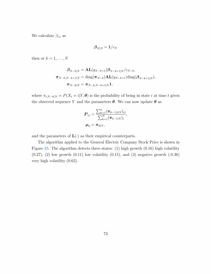
We calculate βi,t as
βN |N = 1/cN
then or k = 1, . . . , N
βN−k|N = AL(yN−k+1)βN−k+1|N/cN−k,
πN−k,N−k+1|N = diag(πN−k)AL(yN−k+1)diag(βN−k+1|N),
πN−k|N = πN−k,N−k+1|N1,
where πi,N−k|N = P (Xt = i|Y,θ) is the probability of being in state i at time t given
the observed sequence Y and the parameters θ. We can now update θ as
P ij =
∑nk=1(πk−1,k|N)ij∑Nk=1(πk−1|N)i
,
µ0 = π0|N ,
and the parameters of L(·) as their empirical counterparts.
The algorithm applied to the General Electric Company Stock Price is shown in
Figure 15. The algorithm detects three states: (1) high growth (0.16) high volatility
(0.27), (2) low growth (0.11) low volatility (0.15), and (3) negative growth (-0.36)
very high volatility (0.62).
73
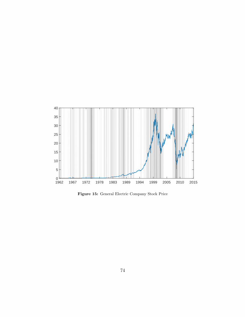
1962 1967 1972 1978 1983 1989 1994 1999 2005 2010 20150
5
10
15
20
25
30
35
40
Figure 15: General Electric Company Stock Price
74
D Continuous- to Discrete-Time Poisson Process
Define the probability of being in state i at time t as Pi(t). With the transition from
state i to j following an exponential distribution with parameter ζij, we can consider
the first-order system equations for the n-state system expressed in matrix form as
ζTP =
−ζ1 ζ12 · · · ζ1n
ζ21 −ζ2 · · · ζ2n...
.... . .
...
ζn1 ζn2 · · · −ζn
T
P1
P2
...
PN
=
P1
P2
...
PN
= P
where
ζi =∑j 6=i
ζij.
The general solution to this homogeneous linear system with constant coefficients
is
P(t) = h1eλ1tc1 + . . .+ hne
λntcn = HΛ(t)c
where (λ1,h1), . . ., (λn,hn) are the eigenpairs of ζT with n independent eigenvectors,
and
H = [h1, . . . ,hn],
c = [c1, . . . , cn]T,
Λ(t) = diag([eλ1t, . . . , eλnt
]).
We can find c with the initial condition P(0) solving
c = H−1P(0).
75

Thus we can get the discrete-time transition matrix Π according to
Π = (H−1)TΛ(1/12)HT.
76
E The Credit Spread Common Factor and the Ex-
cess Bond Premium
In the main text, I show how a single common factor is driving credit spreads,
leverage, and equity return volatility. In this appendix, I will uncover the credit
spreads common factor and show how it relates to the excess bond premium of
Gilchrist and Zakrajsek (2012), firms’ leverage, and firms’ equity return volatility
using more convoluted arguments than a simple principal component analysis of
these series.
Following Gilchrist and Zakrajsek (2012), I want to decompose credit spreads into
(1) a component that captures the systematic movements in default risk of individual
firms and (2) a residual component – sometimes called the excess bond premium –
that represents the time variation in the average price of bearing exposure to US
corporate credit risk, above and beyond the compensation for expected defaults.
However, if some variables that proxies for credit risk are highly correlated with the
excess bond premium, such an estimation cannot be done consistently by taking
the average of the error term of a panel regression of credits spreads on credit risk
variables. Indeed, in that case, the exogeneity condition of the error term will be
violated. As I showed in Section 3, credit spreads are highly correlated with aggregate
firm leverage and aggregate equity return volatility, themselves important indicators
of credit risk. Therefore, I estimate the common factor in corporate bond credit
spreads – the common time varying fluctuations in credit spreads not explained by
cross-sectional differences in credit risk variables – by using a time fixed effect. This
time fixed effect will absorb any effect coming from aggregate time varying changes,
whether it comes from changes in aggregate firms’ credit risk or from a bond risk
premium. In section 6, I resort to a structural approach to decompose aggregate
credit spreads into these two components.
The log of the option adjusted credit spread issued by firm i at time t is assumed
to be related linearly to a vector of firm- and bond-specific characteristic xit that
77
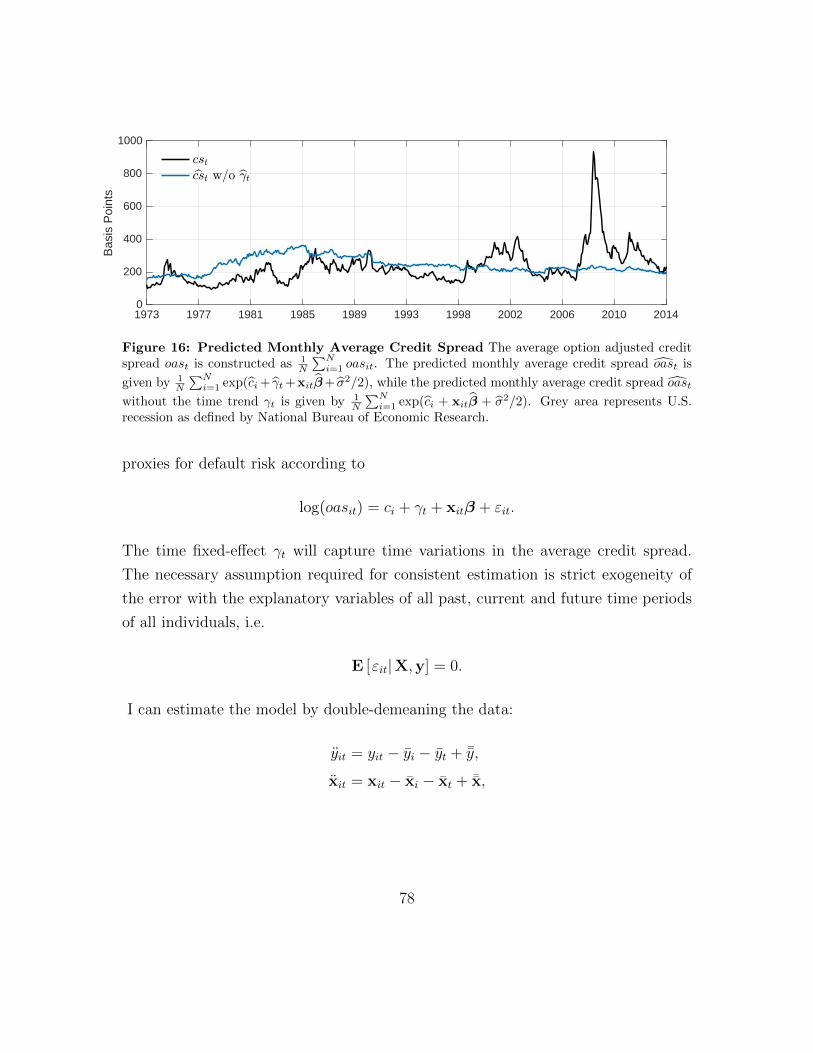
1973 1977 1981 1985 1989 1993 1998 2002 2006 2010 20140
200
400
600
800
1000
Bas
is P
oint
s
cstbcst w/o b.t
Figure 16: Predicted Monthly Average Credit Spread The average option adjusted creditspread oast is constructed as 1
N
∑Ni=1 oasit. The predicted monthly average credit spread oast is
given by 1N
∑Ni=1 exp(ci+ γt+xitβ+ σ2/2), while the predicted monthly average credit spread oast
without the time trend γt is given by 1N
∑Ni=1 exp(ci + xitβ + σ2/2). Grey area represents U.S.
recession as defined by National Bureau of Economic Research.
proxies for default risk according to
log(oasit) = ci + γt + xitβ + εit.
The time fixed-effect γt will capture time variations in the average credit spread.
The necessary assumption required for consistent estimation is strict exogeneity of
the error with the explanatory variables of all past, current and future time periods
of all individuals, i.e.
E [εit|X,y] = 0.
I can estimate the model by double-demeaning the data:
yit = yit − yi − yt + ¯y,
xit = xit − xi − xt + ¯x,
78
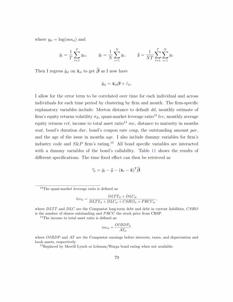
where yit = log(oasit) and
yi =1
T
T∑t=1
yit, yt =1
N
N∑i=1
yi, ¯y =1
NT
T∑t=1
N∑i=1
yi.
Then I regress yit on xit to get β as I now have
yit = xitβ + εit.
I allow for the error term to be correlated over time for each individual and across
individuals for each time period by clustering by firm and month. The firm-specific
explanatory variables include: Merton distance to default dd, monthly estimate of
firm’s equity returns volatility σE, quasi-market leverage ratio13 lev, monthly average
equity returns ret, income to total asset ratio14 inc, distance to maturity in months
mat, bond’s duration dur, bond’s coupon rate coup, the outstanding amount par,
and the age of the issue in months age. I also include dummy variables for firm’s
industry code and S&P firm’s rating.15 All bond specific variables are interacted
with a dummy variables of the bond’s callability. Table 11 shows the results of
different specifications. The time fixed effect can then be retrieved as
γt = yt − ¯y − (xt − ¯x)Tβ.
13The quasi-market leverage ratio is defined as:
levit =DLTTit +DLCit
DLTTit +DLCit + CSHOit × PRCCit,
where DLTT and DLC are the Compustat long-term debt and debt in current liabilities, CSHOis the number of shares outstanding and PRCC the stock price from CRSP.
14The income to total asset ratio is defined as:
incit =OIBDPitATit
where OIBDP and AT are the Compustat earnings before interests, taxes, and depreciation andbook assets, respectively.
15Replaced by Merrill Lynch or Lehman/Warga bond rating when not available.
79
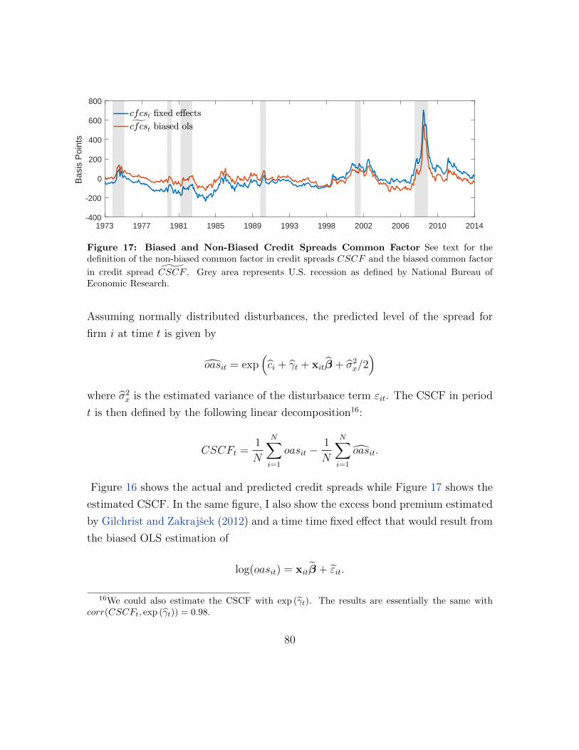
1973 1977 1981 1985 1989 1993 1998 2002 2006 2010 2014-400
-200
0
200
400
600
800
Bas
is P
oint
s
cfcst -xed e,ectsgcfcst biased ols
Figure 17: Biased and Non-Biased Credit Spreads Common Factor See text for thedefinition of the non-biased common factor in credit spreads CSCF and the biased common factor
in credit spread CSCF . Grey area represents U.S. recession as defined by National Bureau ofEconomic Research.
Assuming normally distributed disturbances, the predicted level of the spread for
firm i at time t is given by
oasit = exp(ci + γt + xitβ + σ2
x/2)
where σ2x is the estimated variance of the disturbance term εit. The CSCF in period
t is then defined by the following linear decomposition16:
CSCFt =1
N
N∑i=1
oasit −1
N
N∑i=1
oasit.
Figure 16 shows the actual and predicted credit spreads while Figure 17 shows the
estimated CSCF. In the same figure, I also show the excess bond premium estimated
by Gilchrist and Zakrajsek (2012) and a time time fixed effect that would result from
the biased OLS estimation of
log(oasit) = xitβ + εit.
16We could also estimate the CSCF with exp (γt). The results are essentially the same withcorr(CSCFt, exp (γt)) = 0.98.
80
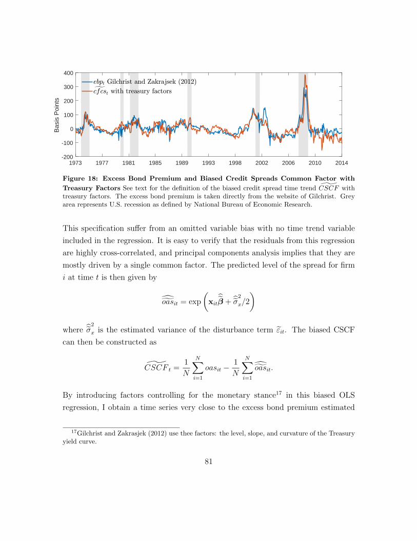
1973 1977 1981 1985 1989 1993 1998 2002 2006 2010 2014-200
-100
0
100
200
300
400
Bas
is P
oint
s
ebpt Gilchrist and Zakrajsek (2012)gcfcst with treasury factors
Figure 18: Excess Bond Premium and Biased Credit Spreads Common Factor with
Treasury Factors See text for the definition of the biased credit spread time trend CSCF withtreasury factors. The excess bond premium is taken directly from the website of Gilchrist. Greyarea represents U.S. recession as defined by National Bureau of Economic Research.
This specification suffer from an omitted variable bias with no time trend variable
included in the regression. It is easy to verify that the residuals from this regression
are highly cross-correlated, and principal components analysis implies that they are
mostly driven by a single common factor. The predicted level of the spread for firm
i at time t is then given by
oasit = exp
(xitβ + σ2
x/2
)
where σ2
x is the estimated variance of the disturbance term εit. The biased CSCF
can then be constructed as
CSCF t =1
N
N∑i=1
oasit −1
N
N∑i=1
oasit.By introducing factors controlling for the monetary stance17 in this biased OLS
regression, I obtain a time series very close to the excess bond premium estimated
17Gilchrist and Zakrasjek (2012) use thee factors: the level, slope, and curvature of the Treasuryyield curve.
81
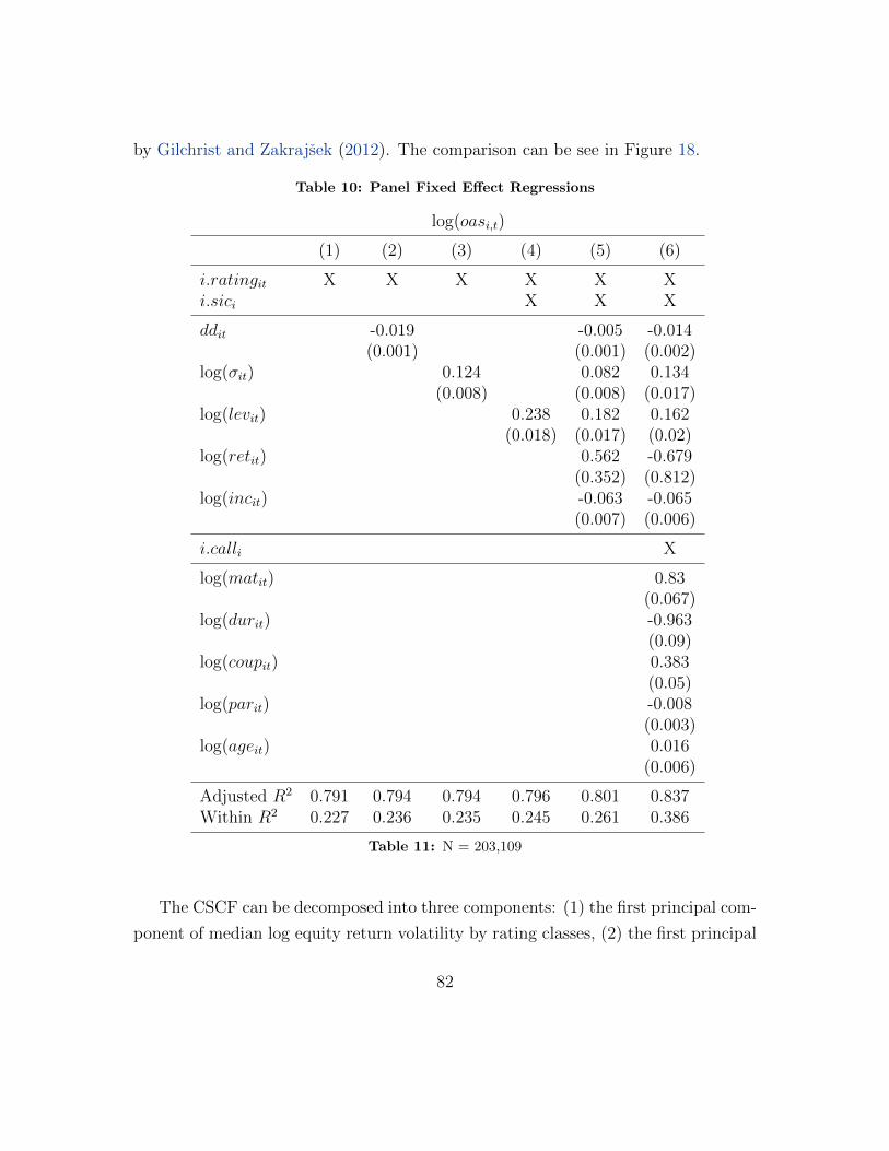
by Gilchrist and Zakrajsek (2012). The comparison can be see in Figure 18.
Table 10: Panel Fixed Effect Regressions
log(oasi,t)
(1) (2) (3) (4) (5) (6)
i.ratingit X X X X X Xi.sici X X X
ddit -0.019 -0.005 -0.014(0.001) (0.001) (0.002)
log(σit) 0.124 0.082 0.134(0.008) (0.008) (0.017)
log(levit) 0.238 0.182 0.162(0.018) (0.017) (0.02)
log(retit) 0.562 -0.679(0.352) (0.812)
log(incit) -0.063 -0.065(0.007) (0.006)
i.calli X
log(matit) 0.83(0.067)
log(durit) -0.963(0.09)
log(coupit) 0.383(0.05)
log(parit) -0.008(0.003)
log(ageit) 0.016(0.006)
Adjusted R2 0.791 0.794 0.794 0.796 0.801 0.837Within R2 0.227 0.236 0.235 0.245 0.261 0.386
Table 11: N = 203,109
The CSCF can be decomposed into three components: (1) the first principal com-
ponent of median log equity return volatility by rating classes, (2) the first principal
82
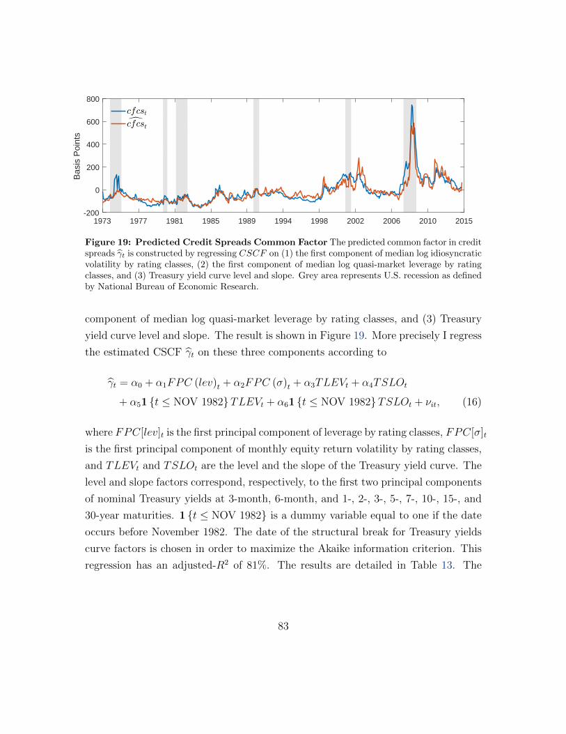
1973 1977 1981 1985 1989 1994 1998 2002 2006 2010 2015-200
0
200
400
600
800
Bas
is P
oint
s
cfcstdcfcst
Figure 19: Predicted Credit Spreads Common Factor The predicted common factor in creditspreads γt is constructed by regressing CSCF on (1) the first component of median log idiosyncraticvolatility by rating classes, (2) the first component of median log quasi-market leverage by ratingclasses, and (3) Treasury yield curve level and slope. Grey area represents U.S. recession as definedby National Bureau of Economic Research.
component of median log quasi-market leverage by rating classes, and (3) Treasury
yield curve level and slope. The result is shown in Figure 19. More precisely I regress
the estimated CSCF γt on these three components according to
γt = α0 + α1FPC (lev)t + α2FPC (σ)t + α3TLEVt + α4TSLOt
+ α51 t ≤ NOV 1982TLEVt + α61 t ≤ NOV 1982TSLOt + νit, (16)
where FPC[lev]t is the first principal component of leverage by rating classes, FPC[σ]t
is the first principal component of monthly equity return volatility by rating classes,
and TLEVt and TSLOt are the level and the slope of the Treasury yield curve. The
level and slope factors correspond, respectively, to the first two principal components
of nominal Treasury yields at 3-month, 6-month, and 1-, 2-, 3-, 5-, 7-, 10-, 15-, and
30-year maturities. 1 t ≤ NOV 1982 is a dummy variable equal to one if the date
occurs before November 1982. The date of the structural break for Treasury yields
curve factors is chosen in order to maximize the Akaike information criterion. This
regression has an adjusted-R2 of 81%. The results are detailed in Table 13. The
83
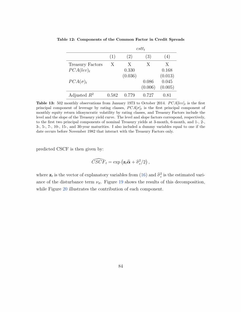
Table 12: Components of the Common Factor in Credit Spreads
csttt
(1) (2) (3) (4)
Treasury Factors X X X XPCA(lev)t 0.330 0.168
(0.036) (0.013)PCA(σ)t 0.086 0.045
(0.006) (0.005)
Adjusted R2 0.582 0.779 0.727 0.81
Table 13: 502 monthly observations from January 1973 to October 2014. PCA[lev]t is the firstprincipal component of leverage by rating classes, PCA[σ]t is the first principal component ofmonthly equity return idiosyncratic volatility by rating classes, and Treasury Factors include thelevel and the slope of the Treasury yield curve. The level and slope factors correspond, respectively,to the first two principal components of nominal Treasury yields at 3-month, 6-month, and 1-, 2-,3-, 5-, 7-, 10-, 15-, and 30-year maturities. I also included a dummy variables equal to one if thedate occurs before November 1982 that interact with the Treasury Factors only.
predicted CSCF is then given by:
CSCF t = exp(ztα+ σ2
z/2),
where zt is the vector of explanatory variables from (16) and σ2z is the estimated vari-
ance of the disturbance term νit. Figure 19 shows the results of this decomposition,
while Figure 20 illustrates the contribution of each component.
84
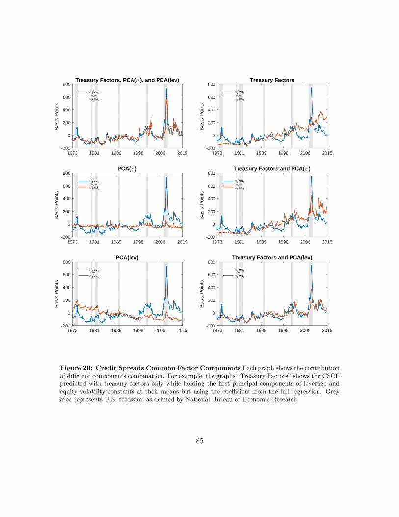
1973 1981 1989 1998 2006 2015-200
0
200
400
600
800
Bas
is P
oint
s
Treasury Factors, PCA(< ), and PCA(lev)
cfcstdcfcst
1973 1981 1989 1998 2006 2015-200
0
200
400
600
800
Bas
is P
oint
s
Treasury Factors
cfcstdcfcst
1973 1981 1989 1998 2006 2015-200
0
200
400
600
800
Bas
is P
oint
s
PCA(< )
cfcstdcfcst
1973 1981 1989 1998 2006 2015-200
0
200
400
600
800
Bas
is P
oint
s
PCA(lev)
cfcstdcfcst
1973 1981 1989 1998 2006 2015-200
0
200
400
600
800
Bas
is P
oint
s
Treasury Factors and PCA(< )
cfcstdcfcst
1973 1981 1989 1998 2006 2015-200
0
200
400
600
800
Bas
is P
oint
s
Treasury Factors and PCA(lev)
cfcstdcfcst
Figure 20: Credit Spreads Common Factor Components Each graph shows the contributionof different components combination. For example, the graphs “Treasury Factors” shows the CSCFpredicted with treasury factors only while holding the first principal components of leverage andequity volatility constants at their means but using the coefficient from the full regression. Greyarea represents U.S. recession as defined by National Bureau of Economic Research.
85
F Approximation to Aggregate Asset Volatility
This appendix details the approximation used in Section 7. The environment is
consistent with Modigliani and Miller’s (1958) theorem. Define yt to be the level of
cash flows generated by firm’s assets:
dytyt
= µY,Fdt+ σY,AdZAt
where ZAt is a Brownian motion representing aggregate shocks. Assume that cor-
porate debt is a perpetual bond with coupon rate c and that there is no option to
default. Investors assume that aggregate asset volatility and the risk-free rate are
constant over time. The valuation of equity by a risk-neutral investor is then given
by
E =yt
r − µ−D
where the perpetual bond value is given by
D =c
r.
Aggregate equity volatility then satisfy
σE,A =E +D
EσY,A.
86
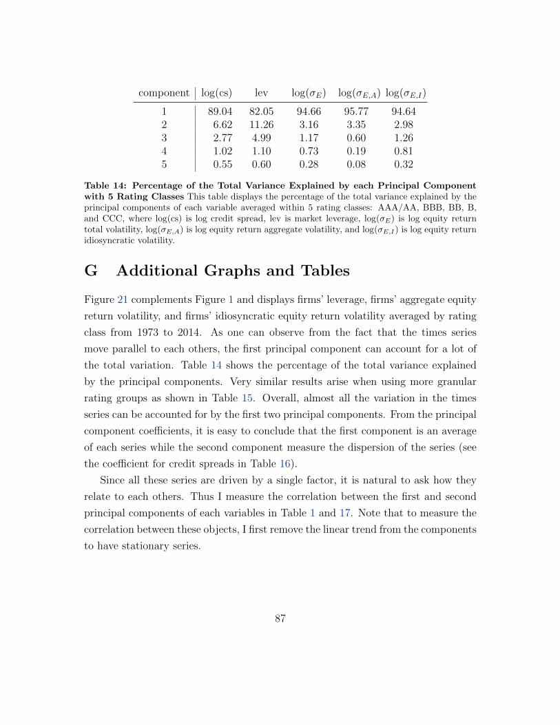
component log(cs) lev log(σE) log(σE,A) log(σE,I)
1 89.04 82.05 94.66 95.77 94.642 6.62 11.26 3.16 3.35 2.983 2.77 4.99 1.17 0.60 1.264 1.02 1.10 0.73 0.19 0.815 0.55 0.60 0.28 0.08 0.32
Table 14: Percentage of the Total Variance Explained by each Principal Componentwith 5 Rating Classes This table displays the percentage of the total variance explained by theprincipal components of each variable averaged within 5 rating classes: AAA/AA, BBB, BB, B,and CCC, where log(cs) is log credit spread, lev is market leverage, log(σE) is log equity returntotal volatility, log(σE,A) is log equity return aggregate volatility, and log(σE,I) is log equity returnidiosyncratic volatility.
G Additional Graphs and Tables
Figure 21 complements Figure 1 and displays firms’ leverage, firms’ aggregate equity
return volatility, and firms’ idiosyncratic equity return volatility averaged by rating
class from 1973 to 2014. As one can observe from the fact that the times series
move parallel to each others, the first principal component can account for a lot of
the total variation. Table 14 shows the percentage of the total variance explained
by the principal components. Very similar results arise when using more granular
rating groups as shown in Table 15. Overall, almost all the variation in the times
series can be accounted for by the first two principal components. From the principal
component coefficients, it is easy to conclude that the first component is an average
of each series while the second component measure the dispersion of the series (see
the coefficient for credit spreads in Table 16).
Since all these series are driven by a single factor, it is natural to ask how they
relate to each others. Thus I measure the correlation between the first and second
principal components of each variables in Table 1 and 17. Note that to measure the
correlation between these objects, I first remove the linear trend from the components
to have stationary series.
87
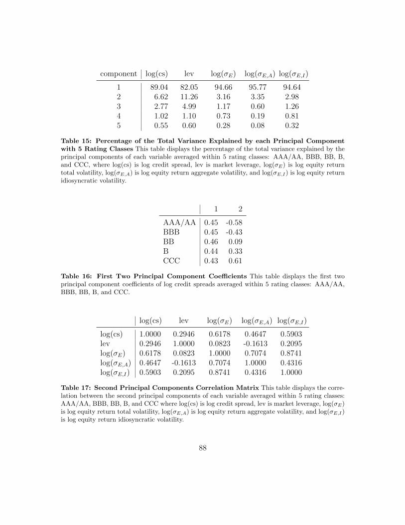
component log(cs) lev log(σE) log(σE,A) log(σE,I)
1 89.04 82.05 94.66 95.77 94.642 6.62 11.26 3.16 3.35 2.983 2.77 4.99 1.17 0.60 1.264 1.02 1.10 0.73 0.19 0.815 0.55 0.60 0.28 0.08 0.32
Table 15: Percentage of the Total Variance Explained by each Principal Componentwith 5 Rating Classes This table displays the percentage of the total variance explained by theprincipal components of each variable averaged within 5 rating classes: AAA/AA, BBB, BB, B,and CCC, where log(cs) is log credit spread, lev is market leverage, log(σE) is log equity returntotal volatility, log(σE,A) is log equity return aggregate volatility, and log(σE,I) is log equity returnidiosyncratic volatility.
1 2
AAA/AA 0.45 -0.58BBB 0.45 -0.43BB 0.46 0.09B 0.44 0.33CCC 0.43 0.61
Table 16: First Two Principal Component Coefficients This table displays the first twoprincipal component coefficients of log credit spreads averaged within 5 rating classes: AAA/AA,BBB, BB, B, and CCC.
log(cs) lev log(σE) log(σE,A) log(σE,I)
log(cs) 1.0000 0.2946 0.6178 0.4647 0.5903lev 0.2946 1.0000 0.0823 -0.1613 0.2095log(σE) 0.6178 0.0823 1.0000 0.7074 0.8741log(σE,A) 0.4647 -0.1613 0.7074 1.0000 0.4316log(σE,I) 0.5903 0.2095 0.8741 0.4316 1.0000
Table 17: Second Principal Components Correlation Matrix This table displays the corre-lation between the second principal components of each variable averaged within 5 rating classes:AAA/AA, BBB, BB, B, and CCC where log(cs) is log credit spread, lev is market leverage, log(σE)is log equity return total volatility, log(σE,A) is log equity return aggregate volatility, and log(σE,I)is log equity return idiosyncratic volatility.
88
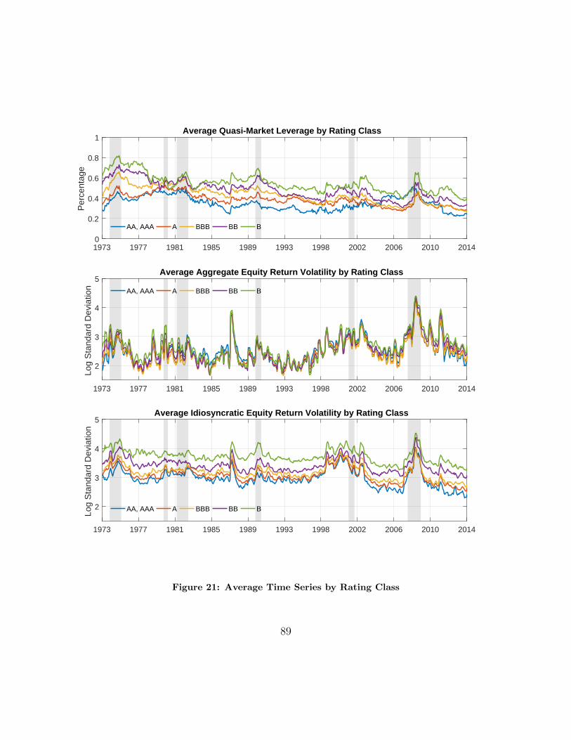
1973 1977 1981 1985 1989 1993 1998 2002 2006 2010 20140
0.2
0.4
0.6
0.8
1
Per
cent
age
Average Quasi-Market Leverage by Rating Class
AA, AAA A BBB BB B
1973 1977 1981 1985 1989 1993 1998 2002 2006 2010 2014
2
3
4
5
Log
Sta
ndar
d D
evia
tion
Average Aggregate Equity Return Volatility by Rating Class
AA, AAA A BBB BB B
1973 1977 1981 1985 1989 1993 1998 2002 2006 2010 2014
2
3
4
5
Log
Sta
ndar
d D
evia
tion
Average Idiosyncratic Equity Return Volatility by Rating Class
AA, AAA A BBB BB B
Figure 21: Average Time Series by Rating Class
89
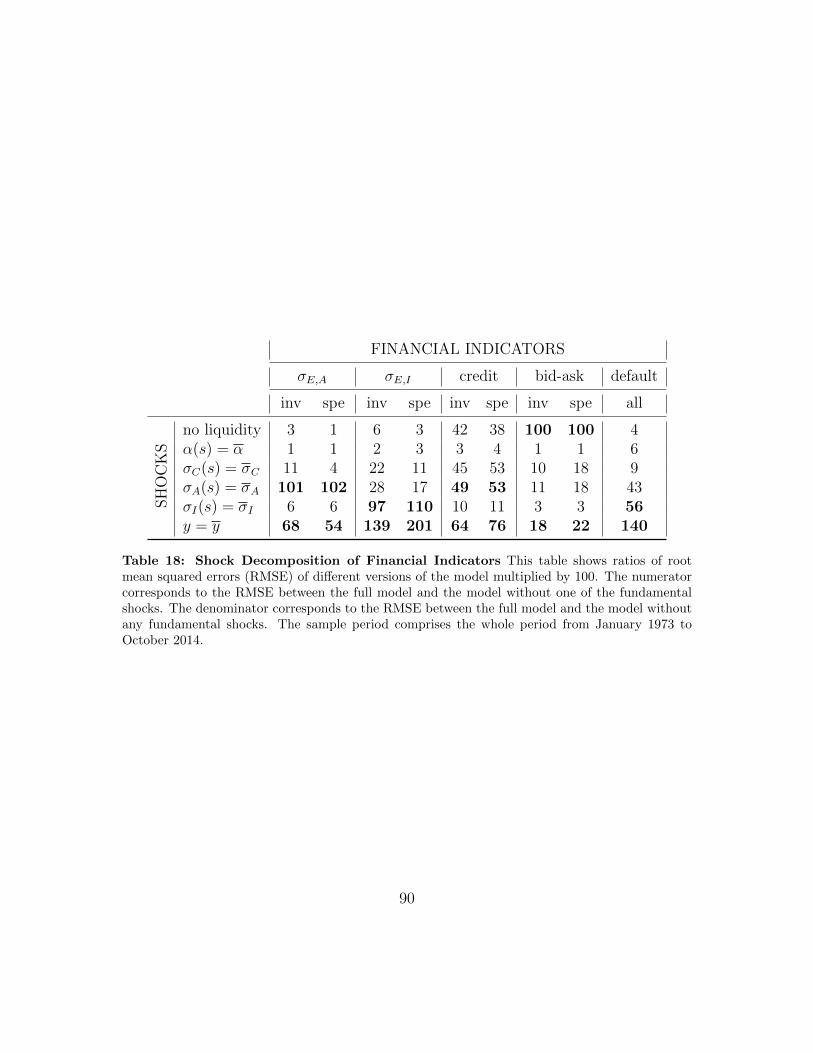
FINANCIAL INDICATORS
σE,A σE,I credit bid-ask default
inv spe inv spe inv spe inv spe all
SH
OC
KS
no liquidity 3 1 6 3 42 38 100 100 4α(s) = α 1 1 2 3 3 4 1 1 6σC(s) = σC 11 4 22 11 45 53 10 18 9σA(s) = σA 101 102 28 17 49 53 11 18 43σI(s) = σI 6 6 97 110 10 11 3 3 56y = y 68 54 139 201 64 76 18 22 140
Table 18: Shock Decomposition of Financial Indicators This table shows ratios of rootmean squared errors (RMSE) of different versions of the model multiplied by 100. The numeratorcorresponds to the RMSE between the full model and the model without one of the fundamentalshocks. The denominator corresponds to the RMSE between the full model and the model withoutany fundamental shocks. The sample period comprises the whole period from January 1973 toOctober 2014.
90