Discussion Paper No.299

Hiroki Murakami Faculty of Economics, Chuo University

January 2018

INSTITUTE OF ECONOMIC RESEARCH Chuo University

Tokyo, Japan

A note on the “unique” business cycle in the Keynesian theory

A note on the “unique” business cycle in the Keynesian theory

Hiroki Murakami∗

Faculty of Economics, Chuo University†

January 25, 2018

Abstract

In this paper, we explore the existence and “uniqueness” of a limit cycle in a Keynesian model of business

cycles. In a model with the simplest (linear) Keynesian consumption function and the logistic investment function

based upon the profit principle, we establish the existence of a periodic orbit (irrespective of the speed of quantity

adjustment) and verify, with the help of the theory on generalized Lienard systems, the uniqueness of it for the

case in which the speed of quantity adjustment is large enough.

Keywords: Generalized Lienard systems; Keynesian economics; Limit cycles; Uniqueness

JEL classification: E12; E32; E37

1 Introduction

It is one of the ultimate objectives of macroeconomics to banish recession and depression all time from economies. In

the midst of the Great Depression in the 1930s, Keynes (1936) intended to establish the “general theory” of output

as a whole and employment to diagnose the contemporary economic conditions and prescribe appropriate policies.1

Inspired by Keynes (1936), several economists proposed theories of business cycles as ups and downs of aggregate

output from the 1930s to the 1950s. Typical examples of them include the theory based upon the multiplier theory

and the profit principle of investment (cf. Kalecki 1939; Kaldor 1940) and the so-called multiplier-accelerator one

(cf. Harrod 1936; Samuelson 1939; Metzler 1941; Hicks 1950; Goodwin 1951; Phillips 1954). The common aim of

these theories is to explore the mechanism of cyclical fluctuations of aggregate output.

In the theory of business cycles, they are usually represented by periodic orbits including limit cycles. It has

widely been recognized that the concept of “nonlinearity” is an essential element in establishing the existence of

periodic orbits. Indeed, Kaldor (1940), Hicks (1950) and Goodwin (1951) noticed the importance of nonlinearity in

∗E-mail: hmura@tamacc.chuo-u.ac.jp†742-1, Higashi-Nakano, Hachioji, Tokyo 192-0393, Japan.1To be fair, Kalecki (1933, 1935) preceded Keynes (1936) in the establishment of the principle of effective demand. Furthermore, his

main concern in these papers was the phenomena of business cycles like ours.

1

theory of business cycles, and several economists initiated rigorous mathematical investigations of the possibility of

generation of periodic orbits by making use of the nonlinear theory of oscillations in as early as the 1950s (cf. Yasui

1953; Ichimura 1955; Morishima 1959).2 From the late 1960s or the 1970s on, the Poincare-Bendixson theorem

or the Hopf bifurcation theorem has also been employed as a mathematical tool for establishing the existence of

periodic orbits (cf. Rose 1967; Chang and Smyth 1971; Torre 1977; Varian 1979). Now it is widely regarded among

economists as the main purpose of theory of business cycles to verify the existence of periodic orbits by utilizing

nonlinear properties in economic models, and there have been a lot of papers which expound the mechanism of

business cycles by taking this method.

Even if the existence of a periodic orbit can be established, however, the uniqueness of it is not necessarily

guaranteed. Unless this uniqueness is ensured, states of economies may converge to different periodic orbits and

amplitudes of fluctuations may differ depending upon initial conditions. These consequences due to multiplicity

of periodic orbits are not favorable for fuller elucidation of the mechanism of business cycles or for applications

to predictions.3 The uniqueness of a periodic orbit is thus a desirable result in the theory of business cycles.

Unfortunately, it has rarely been explored due to technical difficulties. Notable exceptional works on this subject

are Ichimura (1955), Lorenz (1986, 1993), Galeotti and Gori (1989) and Sasakura (1996). Ichimura (1955), Lorenz

(1986, 1993) and Galeotti and Gori (1989) examined the uniqueness of a periodic orbit in Kaldor’s (1940) theory of

business cycles, while Lorenz (1986, 1993) and Sasakura (1996) did in the multiplier-accelerator theory elaborated

by Hicks (1950), Goodwin (1951) or Phillips (1954). Methodologically, they reduced their models of business cycles

to Lienard systems to apply some theorems on the uniqueness of a limit cycle in the systems (cf. Levinson and

Smith 1942; Ye 1986; Zeng et al. 1994). With the help of the theory on Lienard systems, they were able to

establish the uniqueness of a limit cycle, but all of them, except for Sasakura (1996), had to introduce some ad

hoc assumptions. Indeed, Ichimura (1954), Lorenz (1986, 1993) and Galeotti and Gori (1989) assumed that the

investment function is linear with respect to capital stock and that the saving function has an inverse sigmoid shape

with respect to aggregate income, but, as Lorenz (1993) argued, these assumptions are difficult to support from

empirical viewpoints. On the other hand, Sasakura (1996) employed Goodwin’s (1951) piecewise linear investment

function based upon the accelerator principle, but, as Kaldor (1951) pointed out, the accelerator principle itself,

compared with the profit principle, may not be convincing from Keynesian viewpoints.4 Thus, it is worthwhile

to reconsider the possibility of the uniqueness of a limit cycle (or of a persistent business cycle) in more realistic

situations.

2For details on the contributions made by these Japanese economists to economic dynamics, see for instance, Velupillai (2008) orAsada (2014).

3Puu (1986), Matsumoto (2009) and Dohtani (2010) examined the possibility of the multiplicity of limit cycles (by way of thePoincare-Bendixson theorem and of the Hopf bifurcation theorem) in two-dimensional economic models. Their contributions mayindicate the difficulty in obtaining the uniqueness of a periodic orbit.

4In reviewing Hicks’ (1950) theory of business cycles, Kaldor (1951) argued that the profit principle is more akin to Keynes’ (1936)marginal efficiency theory of investment and more plausible from theoretical and empirical viewpoints than the acceleration principleis, because the level of investment is supposed to be related to the level of investment to aggregate income (or profit) in the former,while to a change in aggregate income in the latter.

2

The purpose of this paper is to examine if the uniqueness of a limit cycle can be obtained in the Keynesian

system under reasonable postulates. In Section 2, we set up a Keynesian model of business cycles, which is composed

of differential equations of aggregate income (or of the output-capital ratio) and of aggregate capital stock. In so

doing, we adopt the simplest (linear) Keynesian consumption function, unlike in Ichimura (1955), Lorenz (1986,

1993) and Galeotti and Gori (1989), and the logistic investment (precisely capital formation) function based upon

the profit principle, unlike in Sasakura (1996). In particular, we make a justification of our investment function

by the “binary-choice” treatment. In Section 3, we analyze our Keynesian model by reducing it to a generalized

Lienard system (cf. Zeng et al. 1994; Xiao and Zhang 2003, 2008). By so doing, we establish the existence of a

periodic orbit and verify the uniqueness of it for the case in which the speed of quantity adjustment is fast enough.

In Section 4, we summarize our analysis and conclude this paper.

2 The model

In this section, we set up a Keynesian model of business cycles. The model is consists of several parts: consumption

and investment functions and differential equations of aggregate income (or output) and of capital stock.

2.1 Consumption

We describe aggregate consumption behavior by the following consumption function:

C = C0 + cY, (1)

where c and C0 are positives constant with c < 1. In (1), Y and C denote aggregate income and aggregate

consumption, respectively; c is the marginal propensity to consume; C0 represents the base or fundamental level of

consumption. The consumption function in (1) is in the simplest Keynesian form.

2.2 Investment

To describe aggregate investment behavior, we formalize the following investment function:

I

K= f

( YK

). (2)

In (2), I and K stand for aggregate gross investment and capital stock, respectively; f is the gross capital formation

function. Equation (2) simply states that the rate of gross capital formation I/K is related to the output-capital

ratio Y/K, which can also be regarded as the rate of utilization.5 Also, this formulation is based upon the profit

5If the level of potential output is proportional to that of capital stock, the rate of utilization is also proportional to the output-capitalratio.

3

principle.6

We specify the capital formation function f . To do so, we lay the hypothetical postulate that all firms can

choose only two types of investment behavior: “optimistic” and “pessimistic” plans. If a firm opts the “optimistic”

plan, this firm is assumed to invest the portion δ + µ of its capital stock for the present gross capital formation,

while, in the case of picking the “pessimistic” plan, the portion invested on the present gross capital formation

is assumed to be δ − ν, where δ is a positive constant which represents the constant rate of capital depreciation

and µ and ν are positive constants. In other words, we suppose that each firm selects one of the two alternatives,

δ + µ and δ − ν, as its rate of gross capital formation.7 With this hypothetical setting, we intend to describe the

aggregate rate of gross capital formation f as a result of the distribution of firms among the two types of investment

plans. As Aoki and Yoshikawa (2007) and Yoshikawa (2015) insisted, aggregate data as a result of macroeconomic

or collective behavior of heterogeneous agents should be interpreted in terms of “distributions,” and our “binary-

choice” treatment is consistent with this argument. Letting p be the probability of a firm’s choosing the optimistic

plan, p can, because of the law of large numbers, be viewed as the share of firms taking this plan among all firms.

Employing this probability p, the aggregate rate of gross capital formation f can be calculated as follows:

f = p(δ + µ) + (1− p)(δ − ν) (3)

Since p is allowed to vary in [0, 1], any number in [δ − ν, δ + µ] can be realized as the resultant aggregate rate of

gross capital formation f. If δ + µ and δ − ν are regarded as the upper and lower limits of each firm’s rate of gross

capital formation, which are set by, for instance, economic, institutional or physical conditions, this “binary-choice”

hypothesis can describe any feasible outcome of aggregate capital formation.

To give the investment function in the form of (2), we relate the rate of gross capital accumulation f to the

output-capital ratio Y/K. Generally speaking, it is reasonable to think that the probability of choosing the optimistic

plan p is positively affected by the current economic condition. Since all firms are assumed to take one of the two

alternatives and Y/K can be seen as a proxy of the current economic condition, we can provide the following

relationship between Y/K and p:

ln( p

1− p

)= −β0 + β

Y

K, (4)

6The profit principle was first postulated by Kalecki (1935, 1939) and Kaldor (1940, 1951). Our formalization (2) is close to thoseof Kalecki (1935) and of Kaldor (1951). For microeconomic foundation of this principle, see Murakami (2016). When the aggregatecapital share is constant, the profit principle is conceptually identical with the utilization principle (cf. Kalecki 1971; Steindl 1952, 1979;Rowthorn 1981; Sasaki 2014).

7This “binary-choice” treatment was intensively utilized to describe market sentiments by, for instance, Lux (1995) or Brock andHommes (1997) (cf. Franke and Westerhoff 2017). In the context of business cycles, Franke (2012, 2014) and Murakami (2018) madethis type of theoretical treatment for the same purpose as ours.

4

where β and β0 are real constants with β > 0. Substituting (3) in (4) and eliminating p, we can obtain

f( YK

)= δ +

µ− ν exp(β0 − β(Y/K))

1 + exp(β0 − β(Y/K)). (5)

We can thus determine the shape of the capital formation function f.

Therefore, aggregate investment I can be represented in the following form by (2) and (5):

I

K= δ +

µ− ν exp(β0 − β(Y/K))

1 + exp(β0 − β(Y/K)). (6)

2.3 Quantity adjustment

We represent the varying process of the output-capital ratio (or the rate of utilization) Y/K on the basis of the

Keynesian concept of quantity adjustment. Specifically, we assume that the dynamic process of Y/K is given by

the following form:

( YK

)(≡ d( YK

)/dt)

= α(C + I − Y

K

), (7)

where α is a positive constant which measures the speed of quantity (utilization) adjustment. Equation (7) means

that Y/K is changed in response to that difference between aggregate demand (per unit of capital stock) (C+I)/K

and Y/K, which is equal to aggregate excess demand or supply (per unit of capital stock). This is consistent with

the Keynesian principle of effective demand because aggregate demand (per unit of capital stock) induces changes

in aggregate output (per unit of capital stock). Indeed, equation (7) is one of the typical formalizations in the

Keynesian (or Kaleckian) theory.

Taking account of the consumption and investment functions, formulated in (1) and (6), we can reduce (7) to

the following:

( YK

)= α

[δ +

µ− ν exp(β0 − β(Y/K))

1 + exp(β0 − β(Y/K))− s Y

K+C0

K

], (8)

where s = 1− c ∈ (0, 1). Note that s is nothing but the marginal propensity to save.

2.4 Capital formation

We describe aggregate capital formation process by the following equation:

K = I − δK. (9)

5

Equation (9) simply means that capital stock K is varied by the level of investment I net of capital depreciation

δK.

Putting (6) in (9), we can obtain the following simple expression:

K

K=µ− ν exp(β0 − β(Y/K))

1 + exp(β0 − β(Y/K)). (10)

2.5 The full model: System (K)

Combining (8) and (10), we can complete a Keynesian model of business cycles in the following form:

( YK

)= α

[δ +

µ− ν exp(β0 − β(Y/K))

1 + exp(β0 − β(Y/K))− s Y

K+C0

K

], (8)

K

K=µ− ν exp(β0 − β(Y/K))

1 + exp(β0 − β(Y/K)). (10)

In what follows, the system of (8) and (10) is denoted by System (K) (to signify “Keynesian”).

Note that System (K) can be extended to the situation in which the size of population changes with a constant

rate, by reading C0 and δ, respectively, as the base or fundamental level of individual (per capita) consumption and

as the sum of rates of capital depreciation and of population growth. In this case, Y and K should be read as per

capita income and as per capita capital stock, respectively, and periodic orbits generated in System (K) should be

regarded as “growth cycles.”

3 Analysis

We proceed to analyze our System (K) to discuss the possibility of the “unique” business cycle (or “unique” stable

limit cycle) being generated.

3.1 Existence and uniqueness of equilibrium

We define an equilibrium point of System (K) as a point (Y,K) at which Y = K = 0. One can easily find that

d(Y/K)/dt = 0 is also fulfilled at each equilibrium point. Then, an equilibrium point of System (K), (Y ∗,K∗), can

be redefined as a solution of the following simultaneous equations:

0 = δ +µ− ν exp(β0 − β(Y/K))

1 + exp(β0 − β(Y/K))− s Y

K+C0

K,

0 =µ− ν exp(β0 − β(Y/K))

1 + exp(β0 − β(Y/K)).

6

The unique equilibrium point of System (K) can easily be calculated as follows:

(Y ∗,K∗) =( β0 + ln(ν/µ)

s[β0 + ln(ν/µ)]− βδC0,

β

s[β0 + ln(ν/µ)]− βδC0

). (11)

Note that the unique equilibrium point of System (K) is homogeneous of degree one in C0, provided that it exists.

To ensure that the unique equilibrium point (Y ∗,K∗) lies on the domain of R++, we make the following as-

sumption.

Assumption 1. The following condition is satisfied:

β0 >βδ

s− ln

(νµ

). (12)

Under Assumption 1, we can establish the existence and uniqueness of an economically meaningful equilibrium

point in System (K).

3.2 The positivity constraint

Although the unique equilibrium point of System (K) can be proved to be located in R2++, it may be possible that

the value of Y or K is non-positive, for some t ≥ 0, along some solution path of System (K). In other words, it

remains to be seen if every solution path of System (K), (Y (t),K(t)), with an initial condition (Y (0),K(0)) ∈ R2++,

stays in R2++, for all t ≥ 0. We consider this “positivity constraint” problem below.

Since the value of K can easily be shown to be positive all the time along every solution path with every initial

condition of K(0) > 0, it suffices to confirm that Y > 0 for Y = 0 and an arbitrary K > 0, so as to cope with

the “positivity constraint” problem. Due to the positivity of K, we have Y > 0 if and only if Y/K > 0 along

every solution path of System (K). Thus, to solve the “positivity constraint” problem, we only have to ensure that

d(Y/K)/dt > 0 for Y/K = 0 and for every K > 0, or that

( YK

)∣∣∣Y/K=0

= α[δ +

µ− ν exp(β0)

1 + exp(β0)+C0

K

]> 0, (13)

for every K > 0.

Therefore, we should make the following assumption to solve the “positivity constraint” problem:

Assumption 2. The following condition is satisfied:

(δ + µ) + (δ − ν) exp(β0) ≥ 0. (14)

Note that condition (14) is satisfied if δ ≥ ν i.e., if the lower limit of rate of gross capital formation δ − ν is

nonnegative. Since the rate of gross capital formation is nonnegative by definition, Assumption 2 is a reasonable

7

one.

One can easily find that condition (13) is satisfied for all K > 0 under (14). Under Assumption 2, we can assert

that for every initial condition (Y (0),K(0)) ∈ R++, the solution path of System (K), (Y (t),K(t)), stays in R2++ for

all t ≥ 0.8

3.3 System (K) as a generalized Lienard system

To examine the characteristics of System (K), we rewrite it in another form by introducing the following new

variables x and y defined as follows:

x =Y

K− Y ∗

K∗, (15)

y = lnK∗ − lnK, (16)

where (Y ∗,K∗) is the unique equilibrium defined by (11).

Substituting (15) and (16) in System (K) and taking (11) into consideration, we can rewrite System (K) as

follows:

x = φ(y)− F (x), (17)

y = −g(x), (18)

where

g(x) = µνexp(βx)− 1

µ+ ν exp(βx), (19)

F (x) = α[sx− g(x)], (20)

φ(y) = αs[β0 + ln(ν/µ)]− βδ

β[exp(y)− 1]. (21)

In what follows, the system of (17) and (18) with (19)-(21) is denoted by System (K*). As seen in Appendix,

System (K*) can be classified as a generalized Lienard system.9 To scrutinize the characteristics of System (K), we

look into System (K*). Note that the unique equilibrium point of System (K*) is given by (x∗, y∗) = (0, 0).

3.4 Existence of a periodic orbit

We proceed to examine the possibility of existence of a persistent business cycle, represented by a periodic orbit, in

System (K) by investigating this possibility in System (K*). For this purpose, we adopt the following usual method:

8The “positivity constraint” is one kind of “boundary conditions.” Boundary conditions may be related to the existence of anequilibrium point in dynamical systems. For the role of boundary conditions in verifying the existence of an equilibrium point in relatedKeynesian models, see Murakami (2014, 2015, 2017).

9For generalized Lienard systems, see, for instance, Levinson and Smith (1942), Zeng et al. (1994) or Xiao and Zhang (2003, 2008).

8

to check the total (local asymptotic) instability of the unique equilibrium,10 find a (nonempty) positively invariant

compact subset11 of R2 and apply the Poincare-Bendixson theorem to System (K*).

To begin, we have a look at the local asymptotic stability of the unique equilibrium point of System (K*). To

do so, we calculate the Jacobian matrix of System (K*) evaluated at the unique equilibrium (0, 0), denoted by J∗:

J∗ =

α[βµν/(µ+ ν)− s] α{s[β0 + ln(ν/µ)]/β − δ}

−βµν/(µ+ ν) 0

.

The trace and determinant of J∗ are given as follows:

tr J∗ = α( βµν

µ+ ν− s),

det J∗ =αµν

µ+ ν

{s[β0 + ln

(νµ

)]− βδ

}> 0,

where the inequality follows from Assumption 1. Then, the unique equilibrium point is not a saddle point. We

can thus find that, under the following assumption, the unique equilibrium point is locally asymptotically totally

unstable.

Assumption 3. The following condition is satisfied:

s <βµν

µ+ ν. (22)

We explain the economic meaning of this assumption. Noting that the marginal propensity to invest evaluated

at the unique equilibrium is equal to the right hand side of (22) (cf. (5), (6) and (11)), condition (22) requires

that the marginal propensity to invest be larger than that to save at the unique equilibrium, i.e., that the so-

called Keynesian stability condition (cf. Marglin and Bhaduri, 1990) be violated at the unique equilibrium. As

in Kaldor’s (1940) Keynesian model of business cycles, the violation of the Keynesian stability condition (at the

unique equilibrium) plays a vital role in our Keynesian system. Although the Keynesian stability condition has been

known to ensure the stability of the Keynesian system,12 it has recently been argued by some that this condition

is, from an empirical viewpoint, not satisfied at least around the long-run equilibrium.13 In this respect, it is not

unlikely that Assumption 3 holds in reality.

10We mean by the term “total (local asymptotic) instability” that the equilibrium point under consideration is either an unstablenode or an unstable focus, i.e., that the trace and determinant of the Jacobian matrix evaluated at this equilibrium point are bothpositive.

11A closed (usually compact) region D is said to be positively invariant with respect to the dynamical system under consideration ifevery positive semi-trajectory (i.e., every solution path for t ≥ 0) of this system which starts at an arbitrary point in D will remain inD for ever after (i.e., for all t ≥ 0).

12Samuelson (1947, pp. 276-280) was among the first economists who verified that the stability of the Keynesian system is guaranteedby the Keynesian stability condition.

13For example, Skott (2012) insisted on the violation of the Keynesian stability condition (at least around the long-run equilibrium)in practice, from an empirical viewpoint. For debates on the validity of this condition, see, for instance, Hein et al. (2011) or Franke(2017).

9

Next, we check if a (nonempty) compact and positively invariant region exists in System (K*). To this end, we

take a look at the phase diagram of System (K*) illustrated in figure 1 and consider the solution path of System

(K*) with the initial condition (x(0), y(0)) = (−Y ∗/K∗, 0).14 It can easily be found that, with the passage of time,

this path travels from P (−Y ∗/K∗, 0) (at t = 0) to S on the y axis, via the intersection with the y axis or with the

locus of y = 0, denoted by Q, and that with the locus of x = 0, denoted by R, as illustrated in figure 1. Also, we

denote by T the intersection point of the line of x = −Y ∗/K∗ and that parallel with the x axis passing through S.

Then, we can construct the (nonempty) compact domain enclosed by the arc PQRS and the line segments ST and

TP. Denoting this domain by D, we claim that D is positively invariant with respect to System (K*). As we have

seen in Section 3.2, every solution path of System (K*) (x(t), y(t)) satisfies x(t) > −Y ∗/K∗, which corresponds to

Y (t)/K(t) > 0 in System (K), if x(0) > −Y ∗/K∗. Also, we have y > 0 for x < 0. Moreover, no solution path can

cross the arc PQRS because of the uniqueness of a solution path with respect to an initial condition. Therefore,

every solution path of System (L) will stay on D once it enters D, and so D is positively invariant.

*

*O

x

y

P

Q

R

ST

D

�� = 0

−�

�

�� = 0

Figure 1: Phase diagram of System (K*)

We are now ready to prove the existence of a periodic orbit in System (K) by establishing that in System (K*).

In the following proposition, we present this celebrated fact.

Proposition 1. Let Assumptions 1-3 hold. Then, System (K) has at least one periodic orbit on R2++.

15

Proof. Since the unique equilibrium point of System (K*) is locally asymptotically totally unstable under As-

sumption 3 and the compact domain D defined above is positively invariant, we can enclose the equilibrium by a

sufficiently small rectangle and construct a positively invariant, compact domain, denoted by D∗, by eliminating

the interior of the small rectangle from D. It is obvious that the positively invariant set D∗ contains no equilibrium

14It can be proved that this solution path is unique because System (K*) satisfies the Lipschitz condition (cf. Coddington andLevinson 1955, chap. 1) on R2.

15This proposition can also be shown by a direct application of Theorem 1.1 of Xiao and Zhang (2008, p. 302).

10

point, and so we can apply the Poincare-Bendixson theorem (cf. Coddington and Levinson 1955, chap.16) to System

(K*) on D∗ to conclude that System (K*) has at least one periodic orbit on D∗. Note that such a periodic orbit

lies on the domain of x > −Y ∗/K∗ by Assumption 2.

Therefore, System (K) has at least one periodic orbit and such a periodic orbit lies on R2++.

Proposition 1 implies the existence of a persistent business cycle, represented by a periodic orbit, in our Keynesian

System (K) (under reasonable assumptions). As we have seen, the violation of the Keynesian stability condition

(Assumption 3) plays an essential role in ensuring the existence of a persistent business cycle.

3.5 Uniqueness of a limit cycle

We go on to discuss the uniqueness of a persistent business cycle (or of a limit cycle) in System (K) by way of

System (K*). To this end, we refer to the theorem of Xiao and Zhang (2003), which is reproduced as Theorem 1 in

Appendix.

We check if System (K*) fulfills Assumptions 4-6 (in Appendix) required in Theorem 1. To begin, we can easily

find that g, F and φ defined in (19)-(21) are all continuously differentiable on (−∞,∞) and that conditions (30)

and (31) are satisfied for g and φ, respectively (under Assumption 1). Hence, Assumption 4 holds in System (K*)

with x = −∞ and x =∞.

Next, we see if Assumption 5 is fulfilled in System (K*). We can easily calculate F ′(x) as follows:

F ′(x) = α{s− βµν(µ+ ν)

exp(βx)

[µ+ ν exp(βx)]2

}. (23)

Then, F ′(x) = 0 has exactly two roots x′ and x′ given by

x′ =1

βln(µ[β(µ+ ν)− 2s−

√[β(µ+ ν)− 2s]2 − 4s2]

2sν

)< 0, (24)

x′ =1

βln(µ[β(µ+ ν)− 2s+

√[β(µ+ ν)− 2s]2 − 4s2]

2sν

)> 0, (25)

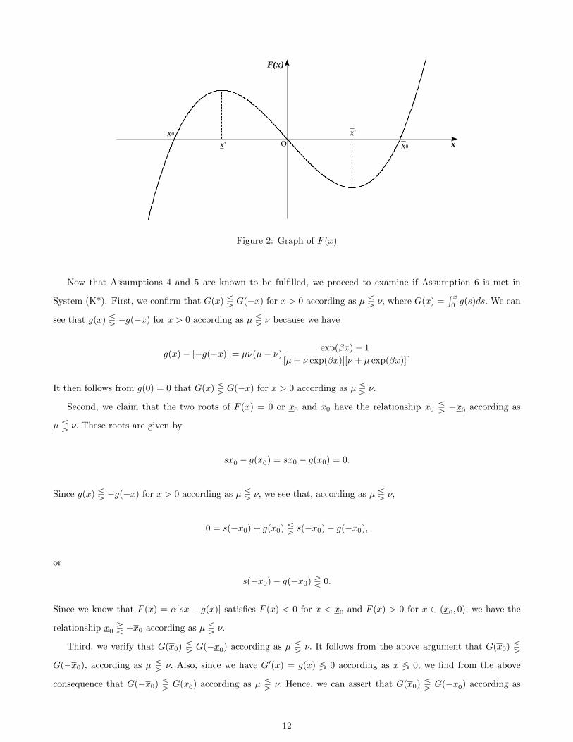
where the inequalities follow from Assumption 3. We can see that F ′(x) > 0 for x < x′ or x > x′ and F ′(x) < 0 for

x ∈ (x′, x′). Hence, we have F (x′) > F (0) = 0 > F (x′). Noting that F (±∞) = ±∞, we can conclude that F (x) = 0

has exactly two roots x0 and x0 besides x = 0 with x0 < x′ < 0 < x′ < x0. Also, it is obvious from (23) that

xF (x) > 0 and F ′(x) ≥ 0 for x < x0 or x > x0. Thus, System (K*) satisfies Assumption 5 under Assumption 3.

11

x

F(x)

Ox'

x' x0

x0

Figure 2: Graph of F (x)

Now that Assumptions 4 and 5 are known to be fulfilled, we proceed to examine if Assumption 6 is met in

System (K*). First, we confirm that G(x) Q G(−x) for x > 0 according as µ Q ν, where G(x) =∫ x

0g(s)ds. We can

see that g(x) Q −g(−x) for x > 0 according as µ Q ν because we have

g(x)− [−g(−x)] = µν(µ− ν)exp(βx)− 1

[µ+ ν exp(βx)][ν + µ exp(βx)].

It then follows from g(0) = 0 that G(x) Q G(−x) for x > 0 according as µ Q ν.

Second, we claim that the two roots of F (x) = 0 or x0 and x0 have the relationship x0 Q −x0 according as

µ Q ν. These roots are given by

sx0 − g(x0) = sx0 − g(x0) = 0.

Since g(x) Q −g(−x) for x > 0 according as µ Q ν, we see that, according as µ Q ν,

0 = s(−x0) + g(x0) Q s(−x0)− g(−x0),

or

s(−x0)− g(−x0) R 0.

Since we know that F (x) = α[sx − g(x)] satisfies F (x) < 0 for x < x0 and F (x) > 0 for x ∈ (x0, 0), we have the

relationship x0 R −x0 according as µ Q ν.

Third, we verify that G(x0) Q G(−x0) according as µ Q ν. It follows from the above argument that G(x0) Q

G(−x0), according as µ Q ν. Also, since we have G′(x) = g(x) ≶ 0 according as x ≶ 0, we find from the above

consequence that G(−x0) Q G(x0) according as µ Q ν. Hence, we can assert that G(x0) Q G(−x0) according as

12

µ Q ν. Note, in particular, that if µ = ν, we have G(x0) = G(x0).

x

g(x)

O

μ

− ν

Figure 3: Graph of g(x)

Fourth, we check that Φ(φ−1(F (x))) is positive and proportional to α for x ∈ (x0, 0) or x ∈ (0, x0), where

Φ(y) =∫ y

0φ(s)ds. It follows from (21) that the inverse function of φ is given by

φ−1(y) = ln(

1 +β

α{s[β0 + ln(ν/µ)]− βδ}y).

Also, we have

Φ(y) =

∫ y

0

φ(s)ds = αs[β0 + ln(ν/µ)]− βδ

β[exp(y)− y − 1].

Hence, we obtain

Φ(φ−1(F (x))) = α{

[sx− g(x)]− s[β0 + ln(ν/µ)]− βδβ

ln(

1 +β

s[β0 + ln(ν/µ)]− βδ[sx− g(x)]

)}= α

s[β0 + ln(ν/µ)]− βδβ

[z − ln(1 + z)],

(26)

where z = β[sx − g(x)]/{s[β0 + ln(ν/µ)] − βδ}. Since F (x) = α[sx − g(x)] 6= 0 for x ∈ (x0, 0) or x ∈ (0, x0) and

z > ln(1 + z) for z 6= 0, it follows from (26) that we obtain the desirable conclusion.

Fifth, we assert that Assumption 6 is fulfilled for α sufficiently large, if µ 6= ν. Since x0 < x′ < 0 < x′ < x0, we

see that

supx∈[0,x0]

(G(x) + Φ(φ−1(F (x)))) ≥ G(x′) + Φ(φ−1(F (x′))),

supx∈[x0,0]

(G(x) + Φ(φ−1(F (x)))) ≥ G(x′) + Φ(φ−1(F (x′))).

13

Then, it suffices for our purpose to show that (noting that G(x0) 6= G(x0) if µ 6= ν)

G(x′) + Φ(φ−1(F (x′))) ≥ G(x0), if G(x0) > G(x0),

G(x′) + Φ(φ−1(F (x′))) ≥ G(x0), if G(x0) > G(x0),

which can, from the above argument, be reduced to

Φ(φ−1(F (x′))) ≥ G(x0)−G(x′), if µ < ν,

Φ(φ−1(F (x′))) ≥ G(x0)−G(x′), if µ > ν,(27)

As we have seen, x0 and x0 are determined independently from α because they are the roots of F (x) = α[sx−g(x)] =

0 and so are x′ and x′ (cf. (24) and (25)). Then, the right hand side of (27) is independent from α in either case

because it is obvious from (19) that G(x) =∫ x

0g(s)ds is also independent from α. On the other hand, since we

know from (26) that Φ(φ−1(F (x′))) and Φ(φ−1(F (x′))) are both positive and proportionate to α, the left hand side

is positive and sufficiently large for α sufficiently large in either case. Thus, we can see that condition (27) holds if

α is sufficiently large.

Therefore, System (K*) fulfills Assumption 6 for α sufficiently large, if µ 6= ν. Note that if µ = ν, Assumption 6

is met irrespective of the value of α > 0 because G(x0) = G(x0).

Now we are ready to establish the following celebrated conclusion on the uniqueness of a limit cycle in System

(K*) or (K).

Proposition 2. Let Assumptions 1-3 hold.

(i) If µ = ν, System (K) has a unique limit cycle on R2++ and it is stable (regardless of the value of α > 0).

(ii) If µ 6= ν, for α sufficiently large, System (K) has a unique limit cycle on R2++ and it is stable.

Proof. Since we have verified the existence of a periodic orbit in System (K) in Proposition 1, it suffices for our

proof to show the uniqueness of a limit cycle obtains in System (K) or (K*) in cases (i) and (ii).

As we have already seen, Assumptions 4-6 are satisfied in cases (i) and (ii). It then follows from Theorem 1 that

the uniqueness of a limit cycle obtains in System (K*) in these cases.

Therefore, the proof is completed.

Proposition 2 states the fact that there exists a “unique” business cycle in our Keynesian System (K), if the

speed of quantity adjustment α is sufficiently large. Since the Keynesian system is characterized by fast quantity

adjustment (cf. Leijonhufvud 1968; Tobin 1993), this proposition indicates the fact that there is universally a unique

business cycle in the Keynesian system. Also, since the uniqueness of a business cycle has seldom been explored, it

may be said that our conclusion is itself “unique.”

It may be better to make some remarks on our conclusion in terms of the mathematical concept of “structural

14

stability.”16 Although we have required in Proposition 2 that α be large enough (for (27) to hold) for the case of

µ 6= ν, this requirement is not necessary if µ and ν are sufficiently close to each other. Since it is not difficult to

prove that System (K*) possesses structural stability if µ = ν, because of the uniqueness and (local asymptotic)

total instability of an equilibrium point and the uniqueness and stability of a limit cycle (cf. Peixoto 1962, p. 104,

Theorem 1.1), we can argue that the uniqueness of a limit cycle is also retained when µ and ν are sufficiently close

to each other. In this respect, we may state that for our Keynesian System (K) to have a unique business cycle, the

speed of quantity adjustment α needs to be larger as µ and ν get farther from each other. Note that it is difficult

(or practically impossible) to calculate the threshold value of α analytically (because of the difficulty in deriving

the values of x0 and of x0) but possible to do numerically.

4 Conclusion

We are in a position to summarize our analysis.

In this paper, we have examined whether a unique limit cycle exists in a Keynesian model of business cycles.

With the simplest linear consumption and logistic investment functions, we have clarified that a unique limit cycle

does exist if the speed of quantity adjustment is fast enough. Moreover, by introducing these functional forms, we

believe, we have been able to remove the ad hoc assumptions in the related preceding works.

Although our analysis has presented an affirmative answer for the question as to the uniqueness of a business

cycle, we have to note that this conclusion is confined to a two-dimensional Keynesian system in which the state

variables are aggregate income and capital stock. If our Keynesian system can be extended to one with more

dimensionality by, for instance, incorporating the Phillips curve,17 the uniqueness of a limit cycle is much harder

to obtain because of the possibility of chaotic motions (especially due to the impossibility of applications of the

Poincare-Bendixson theorem). In this respect, it remains an open question under what conditions the (existence

and) uniqueness of a limit cycle can be gained in more general Keynesian systems.

Acknowledgment

This work was supported by Chuo University Personal Research Grant.

16For details on the mathematical concept of structural stability, see, for instance, DeBaggis (1952) or Peixoto (1962). This conceptwas discussed in several preceding works on economic dynamics (cf. Ichimura 1955; Rose 1967; Chang and Smyth 1971; Velupillai 1979;Flaschel 1984; Lorenz 1993; Sasakura 1994, 1996; Murakami 2014, 2015). It is generally thought among economists that structuralstability is a desirable characteristic which economic models should possess, but as is known, Goodwin’s (1967) model of growth cycles,which can be reduced to a Lotka-Volterra system, is not structurally stable (cf. Velupillai 1979; Flaschel 1984).

17For Keynesian systems with price flexibility or inflation-deflation expectations, see, for instance, Chiarella and Flachel (2000), Asadaet al. (2006), Chiarella et al. (2013), Murakami (2014) or Murakami and Asada (2018). In them, the uniqueness of a limit cycle wasunexplored.

15

Appendix: Generalized Lienard systems

We introduce the theorems by Xiao and Zhang (2003) on the existence and uniqueness of a (stable) limit cycle in

generalized Lienard systems.

We consider the following generalized Lienard system:

x = φ(y)− F (x), (28)

y = −g(x). (29)

In what follows, the system of equations (28) and (29) is denoted by System (L).

Following Xiao and Zhang (2003), we make the following assumptions concerning System (L).

Assumption 4. The real valued functions g(x) and F (x) are, respectively, continuous and continuously differen-

tiable on (x, x), and the real valued function φ(y) is continuously differentiable on (y, y) with −∞ ≤ x < 0 < x ≤ ∞

and −∞ ≤ y < 0 < y ≤ ∞. Moreover, the following conditions are satisfied:

xg(x) > 0 for x 6= 0, (30)

φ(0) = 0, φ′(y) > 0 for y ∈ (y, y). (31)

Assumption 5. There exist x0 and x0 with x < x0 < x0 < x such that the following conditions are satisfied:

F (x0) = F (0) = F (x0) = 0, (32) xF (x) ≤ 0 for x ∈ (x0, x0),

xF (x) > 0, F ′(x) ≥ 0 for x ∈ (x, x0) or x ∈ (x0, x).(33)

Moreover, F (x) is not identically equal to 0 for x sufficiently close to 0.

Assumption 6. The curve of φ(y) = F (x) is well defined for x ∈ [x0, x0].18 Moreover, the following condition is

satisfied:

supx∈[0,x0](G(x) + Φ(φ−1(F (x)))) ≥ G(x0), if G(x0) ≥ G(x0),

supx∈[x0,0](G(x) + Φ(φ−1(F (x)))) ≥ G(x0), if G(x0) > G(x0),

(34)

where G(x) =∫ x

0g(s)ds and Φ(x) =

∫ x

0φ(s)ds.

Assumption 4 is a typical one in the theory of generalized Lienard systems, while Assumptions 5 and 6 concern

the shape of F (x) and those of g(x) and φ(x), respectively.

18Xiao and Zhang (2003) assumed that the curve of φ(y) = F (x) is well defined for x ∈ (x, x), but our assumption suffices for theproof of their theorem (cf. Xiao and Zhang 2003, pp. 1187-1190).

16

Concerning the uniqueness of a periodic orbit or of a limit cycle in System (L), the following theorem was

established by Xiao and Zhang (2003).

Theorem 1. Let Assumptions 4-6 hold. Then, System (L) has at most one limit cycle, and it is stable if it exists.

Proof. See Xiao and Zhang (2003, p. 1187, Theorem 2.2).

References

Aoki, M., Yoshikawa, H., 2007. Reconstructing Macroeconomics: A Perspective from Statistical Physics and

Combinatorial Stochastic Processes. Cambridge University Press, Cambridge.

Asada, T., Chen, P., Chiarella, C., Flaschel, P. 2006. Keynesian dynamics and the wageprice spiral: A baseline

disequilibrium model. Journal of Macroeconomics 28, 90-130.

Asada, T., 2014. Japanese contributions to dynamic economic theories from the 1940s to the 1970s: A historical

survey. Asada, T. (Ed.), The Development of Economics in Japan: From the Inter-war Period to the 2000s.

Routledge, London, pp. 61-89.

Chang, W. W., Smyth, D. J., 1971. The existence and persistence of cycles in a non-linear model: Kaldor’s 1940

model re-examined. Review of Economic Studies 38 (1), 37-44.

Chiarella, C., Flaschel, P., 2000. The Dynamics of Keynesian Monetary Growth: Macro Foundations. Cambridge

University Press, Cambridge.

Chiarella, C., Flaschel, P., Semmler, W., 2013. Reconstructing Keynesian Macroeconomics, Vol. 2. Routledge, New

York.

Coddington, E. A., Levinson, N., 1955. Theory of Ordinary Differential Equations. McGraw Hill, New York.

DeBaggis, H. F., 1952. Dynamical system with stable structures. In: Lefschetz, S. (Ed.), Contribution to the

Theory of Nonlinear Oscillations, vol. 2. Princeton University Press, Princeton, pp. 37-59.

Dohtani, A., 2010. A growth-cycle model of Solow-Swan type, I. Journal of Economic Behavior and Organization

76, 428-444.

Flaschel, P., 1984. Some stability properties of Goodwin’s growth cycle a critical elaboration. Journal of Economics

44 (1), 63-69.

Franke, R., 2012. Microfounded animal spirits in the new macroeconomic consensus. Studies in Nonlinear Dynamics

and Econometrics 6 (4), Article 4.

17

Franke, R., 2014. Aggregate sentiment dynamics: A canonical modelling approach and its pleasant nonlinearities.

Structural Change and Economic Dynamics 31, 64-72.

Franke, R., Westerhoff, F., 2017. Taking stock: A rigorous modelling of animal spirits in macroeconomics. Journal

of Economic Surveys, 31 (5), 1152-1182.

Galeotti, M., Gori, F., 1989. Uniqueness of periodic orbits in Lienard-type business cycle models. Metroeconomica

40 (2), 135-146.

Goodwin, R. M., 1951. The non-linear accelerator and the persistence of business cycles. Econometrica 19 (1),

1-17.

Goodwin, R. M., 1967. A growth cycle. In: Feinstein C. H. (ed.), Socialism, Capitalism and Economic Growth.

Cambridge University Press, Cambridge, pp. 54-58.

Harrod, R. F., 1936. The Trade Cycle: An Essay. Clarendon Press, Oxford.

Hicks, J. R., 1950. A Contribution to the Theory of the Trade Cycle. Clarendon Press, Oxford.

Ichimura, S., 1955. Toward a general nonlinear macrodynamic theory of economic fluctuations. In: K. K. Kurihara

(Ed.), Post Keynesian Economics. New York, Wolff Book Manufacturing, pp. 192-226.

Kaldor, N., 1940. A model of the trade cycle. Economic Journal 50 (192), 78-92.

Kaldor, N., 1951. Mr. Hicks on the trade cycle. Economic Journal 61 (244), 833-847.

Kalecki, M., 1933. Outline of a theory of the business cycle. In: Kalecki, M., Selected Essays on the Dynamics of

the Capitalist Economy 1933-1970. Cambridge University Press, Cambridge, 1971, pp. 1-14.

Kalecki, M., 1935. A macrodynamic theory of business cycles. Econometrica 3 (3), 327-344.

Kalecki, M., 1939. Essays in the theory of economic fluctuations. George and Unwin, London.

Kalecki, M., 1971. Selected Essays on the Dynamics of the Capitalist Economy 1933-1970. Cambridge University

Press, Cambridge.

Keynes, J. M., 1936. The General Theory of Employment, Interest and Money. Macmillan, London.

Leijonhufvud, A., 1968. On Keynesian Economics and the Economics of Keynes: A Study in Monetary Theory.

Oxford University Press, Oxford.

Lorenz, H. W., 1986. On the uniqueness of limit cycles in business cycle theory. Metroeconomica 38 (3), 281-293.

Lorenz, H. W., 1993. Nonlinear Dynamical Economics and Chaotic Motion, 2nd ed. Springer-Verlag, Berlin Hei-

delberg.

18

Lux, T., 1995. Herd behaviour, bubbles and crashes. Economic Journal 105, 881-889.

Marglin, S. A., Bhaduri, A., 1990. Profit squeeze and Keynesian theory. In: Marglin, A., Schor, J. B. (Eds.), The

Golden Age of Capitalism: Reinterpreting the Postwar Experience. Clarendon Press, Oxford, pp. 153- 186.

Matsumoto, A., 2009. Note on Goodwin’s 1951 nonlinear accelerator model with an investment delay. Journal of

Economic Dynamics and Control 33, 832-842.

Metzler, L. A., 1941. The nature and stability of inventory cycles. Review of Economics and Statistics 23 (3),

113-129.

Murakami, H., 2014. Keynesian systems with rigidity and flexibility of prices and inflation-deflation expectations.

Structural Change and Economic Dynamics 30, 68-85.

Murakami, H., 2015. Wage flexibility and economic stability in a non-Walrasian model of economic growth. Struc-

tural Change and Economic Dynamics 32, 25-41.

Murakami, H., 2016. A non-Walrasian microeconomic foundation of the “profit principle” of investment. In: Mat-

sumoto A., Szidarovszky, F., Asada, T. (Eds.), Essays in Economic Dynamics: Theory, Simulation Analysis, and

Methodological Study. Springer, Singapore, pp. 123-141.

Murakami, H., 2017. Time elements and oscillatory fluctuations in the Keynesian macroeconomic system. Studies

in Nonlinear Dynamics and Econometrics 21 (2).

Murakami, H., 2018. A two-sector Keynesian model of business cycles. Metroeconomica, forthcoming.

Murakami, H., Asada, T., 2018. Inflation-deflation expectations and economic stability in a Kaleckian system.

Journal of Economic Dynamics and Control, forthcoming.

Morishima, M., 1959. A contribution to the nonlinear theory of the trade cycle. Journal of Economics 18 (4),

165-173.

Peixoto, M. M., 1962. Structural stability on two-dimensional manifolds. Topology 1 (2), 101-120.

Phillips, A. W., 1954. Stabilisation policies in a closed economy. Economic Journal 64 (254), 290-323.

Puu, T., 1986. Multiplier-accelerator models revisited. Regional Science and Urban Economics 16, 81-95.

Rose, H., 1967. On the non-linear theory of the employment cycle. Review of Economic Studies 34 (2), 153-173.

Rowthorn, R. E., 1981. Demand, real wages and economic growth. Thames Papers in Political Economy 22, 1-39.

Samuelson, P. A., 1939. Interactions between the multiplier analysis and the principle of acceleration. Review of

Economics and Statistics 21 (2), 75-78.

19

Samuelson, P. A., 1947. Foundations of Economic Analysis. Harvard University Press, Cambridge MA.

Sasaki, H., 2014. Growth, Cycles, and Distribution: A Kaleckian Approach. Kyoto University Press, Kyoto.

Sasakura, K., 1994. On the dynamic behavior of Schinasi’s business cycle model. Journal of Macroeconomics 16

(3), 423-444.

Sasakura, K., 1996. The business cycle model with a unique stable limit cycle. Journal of Economic Dynamics and

Control 20, 1763-1773.

Skott, P., 2012. Theoretical and empirical shortcomings of the Kaleckian investment function. Metroeconomica 63

(1), 109-138.

Steindl, J., 1952. Maturity and Stagnation in American Capitalism. Basil Blackwell, Oxford.

Steindl, J., 1979. Stagnation theory and stagnation policy. Cambridge Journal of Economics 3 (1), pp. 1-14.

Tobin, J., 1993. Price flexibility and output stability: an old Keynesian view. Journal of Economic Perspectives 7

(1), 45-65.

Torre, V., 1977. Existence of limit cycles and control in complete Keynesian system by theory of bifurcations.

Econometrica 45 (6), 1457-1466.

Varian, H. R., 1979. Catastrophe theory and the business cycle. Economic Inquiry 17 (1), 14-28.

Velupillai, K. V., 1979. Some stability properties of Goodwin’s growth cycle. Journal of Economics 39 (3-4),

245-257.

Velupillai, K. V., 2008. Japanese contributions to nonlinear cycle theory in the 1950s. Japanese Economic Review

59 (1), 54-74.

Xiao, D., Zhang, Z., 2003. On the uniqueness and nonexistence of limit cycles for predator-prey systems. Nonlin-

earity 16 (3), 1185-1201.

Xiao, D., Zhang, Z., 2008. On the existence and uniqueness of limit cycles for generalized Lienard systems. Journal

of Mathematical Analysis and Applications 343, 299-309.

Yasui, T., 1953. Nonlinear self-excited oscillations and business cycles. Cowels Commission Discussion Papers:

Economics 2065.

Ye, Y., 1986. Theory of Limit Cycles. Translation of Mathematical Monograph 66. American Mathematical Society,

Providence.

20

Yoshikawa, H., 2015. Stochastic macro-equilibrium: a microfoundation for the Keynesian economics. Journal of

Economic Interaction and Coordination 10 (1), 31-55.

Zeng, X., Zhang, Z., Gao, S., 1994. On the uniqueness of the limit cycle of the generalized Lienard equation.

Bulletin of London Mathematical Society 26, 213-247.

21