Discussion Paper No. 132

Regional Economic Integration and its Impacts on

Growth, Poverty and Income Distribution: The Case of Vietnam

by

Tien Dung Nguyen* and Mitsuo Ezaki**

March 2005

* Researcher, Division of Management and System Research, Institute of Information Technology,

Vietnam Institute of Sciences and Technology

** Professor, Graduate School of International Development, Nagoya University

This research was financially supported by the following Grants-in-Aid of Japan Society for the

Promotion of Sciences (JSPS) in the fiscal year 2004:

(1) Grant-in-Aid for Scientific Research (B) (No.16330037), “Regional Economic Integration and

Growth, Income Distribution and Poverty Alleviation in East Asia: Econometric Study based on

CGE Modelling”. Project leader: Mitsuo Ezaki.

(2) Grant-in-Aid for Exploratory Research (No.16663017), “Study on the Method of Relational

Analysis between Trade and Investment Liberalization and Poverty Alleviation under the Global

Economy”. Project leader: Hiroshi Osada.

Abstract The trade liberalization and regional economic integration have recently accelerated in East Asia, with several free trade areas have been established or are under negotiation. As for Vietnam, after acquiring ASEAN membership in 1995, the country has signed a bilateral trade package with the United States and participated in the China-ASEAN free trade area. This paper attempts to analyze impacts on Vietnam of the ongoing regional economic integration, focussing on growth, poverty reductions and income distribution. For this purpose, we have constructed a global linked Computable General Equilibrium (CGE) model and make use of GTAP database version 6.0 and Vietnam’s living standards surveys. The simulation analysis shows that the regional economic integration generally has positive impacts, and it is both welfare enhancing and income-distribution improving for Vietnam. Household income and consumption increase, and poor and rural household groups benefit more than high income urban groups.

Table of Contents 1. Introduction 2. Trade liberalization in Vietnam 3. Poverty and income distribution 4. Model specification 5. Simulation analysis 6. Summary and conclusions References Appendix A: The equation system and model notation Appendix B: The social accounting matrix for Vietnam Appendix C: The elasticities of substitution

1 2 8

11 16 27 28 31 39 48

1

Regional Economic Integration and its Impacts on

Growth, Poverty and Income Distribution:

The Case of Vietnam

Tien Dung Nguyen and Mitsuo Ezaki

1. Introductions

Twenty years have passed since Vietnam began profound social and economic reforms, which

have transformed Vietnam from a centrally planned economy to a market one. Since the

beginning days of the economic reforms, trade reforms and the open-door policies have

constituted an integral part of overall economic reforms. The restrictions and limitations on

trade activities have been steadily and progressively removed, and Vietnam has successfully

developed trade and investment relations with countries in Asia, Europe and North America.

Trade reforms have contributed to the rapid growth of exports and the overall economic growth.

The economic integration with the regional and global economy has recently

accelerated in Vietnam. Vietnam became a member of ASEAN in 1995, joined APEC in 1998,

while negotiating for WTO membership. Vietnam has also concluded a bilateral trade agreement

with the United States in 2000, and has participated in the China-ASEAN free trade area. Given

the national target of sustained growth and poverty alleviation, the Vietnamese policy makers

are greatly concerned with the possible consequences of these liberalization movements on

growth, poverty and income distribution.

This paper attempts to examine the impacts of the ongoing regional economic

integration on Vietnam’s economy using a global Computable General Equilibrium (CGE)

model. The discussion will continue in section 2 analyzing the trade liberalization and regional

economic integration in Vietnam. It is followed by section 3 examining poverty and

income-distribution issues in Vietnam. The structure of the global CGE model is presented in

2

section 4, and simulation scenarios are performed and discussed in section 5. Policy

implications are drawn and some concluding remarks are given in section 6.

2. Trade liberalization in Vietnam

Since the late 1980s, Vietnam’s trade reforms have been progressed steadily, consisting of the

creation and amendment of a system of taxation of imports and exports, the gradual removal of

non-tariff barriers and progressive deregulation of trade regimes. The entry to trading activities

has been liberalized for both state-owned enterprises and private firms. Currently all businesses

are allowed to exports or to imports all goods that are consistent with the field of business

identified in their business registration license. The deregulation of trading rights has increased

the competitiveness and efficiency of trading activities1.

At the same time, a legal system, including a tariff system, has been established to

regulate foreign trade. The tariff system has been simplified and rationalized, and tariff rates

have been lowered. The average weighted tariff rate dropped from nearly 20% in early 1990s to

around 15% in the late 1990s (SRV, 1999). Quantitative restrictions on imports have been

removed for the majority of commodities, with the exception of petroleum products, sugar and

some other strategic products. The surrender requirement and other currency control measures

introduced in 1997 to cope with the East Asian crisis have been eliminated. Foreign-invested

firms are no longer required to balance their foreign exchange account. The number of imports

that subject to the minimum valuation procedure has also reduced considerably.

With respect to exports, export duties and quotas have been removed for the majority

of products. Only a small number of exports are being levied with export taxes mainly for the

purpose of raising revenue, but the tax rates are low. With the exception of some products

regulated due to environmental, health or security concerns, quotas are only imposed on the

1 Vietnam’s trade regimes have been the subject in several studies, such as CIE (1998) and CIE (1999a). The non-tariff barriers that were present in Vietnam by 1999 are surveyed in detail in CIE (1999b) and McCarty (1999)

3

export of garment and textiles to the EU, the United Sates and Canada. These quotas are

imposed by the importing countries, and are determined in the bilateral trade agreements

between Vietnam and these countries. The export quotas on garment and textiles are to be

removed by WTO members in 2005, as mandated by the Agreement on Trade in Textiles (ATC).

However, Vietnam has to acquire WTO membership before it could open the US and EU market

for garment and textile products.

Generally high tariff rates and non-tariff barriers are employed to protect consumer

goods, while capital goods and production inputs are subject to low tariffs and very few

non-tariff barriers. Effective protection provided to many industries is higher than that offered

by nominal protection. Several studies have shown that many industries and consumer goods

industries in particular have enjoyed very high degrees of effective protection2. However,

imports of some intermediate inputs, which are being domestically produced such as cement,

fertilizers, or steal, have been subject to very high tariffs. Protection through tariffs and

non-tariffs barriers is also provided to some so-called infant industries, such as automobile or

petroleum products. The protection of upstream industries, however, raises the price of

intermediate inputs and negatively affects downstream industries and export activities3.

Together with unilateral reform measures, Vietnam has made important commitments

to trade liberalization under various bilateral and multilateral agreements. Vietnam became a

member of ASEAN in 1995, joined APEC in 1998, while applying for the membership of the

WTO. In 2000, Vietnam agreed on a landmark trade package with the United States. Together

with other ASEAN member, Vietnam has participated in the recent formation of a free trade area

between ASEAN and China. All these bilateral and multilateral agreements are being

implemented, and are integral parts of Vietnam’ trade reforms.

2 See, for example, CIE (1998) and Fukase and Martin (1999) for the estimates of effective protection rates by industries. 3 Fukase and Martin (1999) show that exports-oriented industries suffers negative effective protection as protection given to intermediate inputs raises the cost of production.

4

Under the ASEAN free trade area (AFTA), the member countries are obligated to

reduce tariffs on intra-ASEAN trade to less than 5% by the year 2002. As a later member of

ASEAN, Vietnam is allowed to fulfill its commitment to trade liberalization over a longer

period. According to the Common Effective Preferential Tariff (CEPT) agreement, products

with current tariff rates under 20% will have tariffs reduced to 0-5% by the year 2003. For

products with tariffs above 20%, rates are to be reduced to 0-5% by the year 2006. In addition to

the tariff reductions, Vietnam is obligated to remove quantitative restrictions and non-tariff

barriers. The AFTA agreement calls for an immediate elimination of quantitative restrictions as

soon as products are phased in the Inclusion List4.

The implementation of CEPT began in 1996, but progressed slowly until 1999. Most

products that were subject to early tariff cuts were not produced in Vietnam or already had tariff

rate of less than 5% and were subject to very few non-tariff barriers (Tongzon, 1999). Since

2000, tariff reductions have been carried out for highly protected products and are expected to

have greater impact on the economy. When the tariff reduction under AFTA is completed by

2006, over 97% of Vietnam’s tariff lines will have their tariffs reduced to under 5%.

In November 2001, China and ASEAN agreed to establish a free trade area within ten

years, in which tariffs and non-tariff barriers will be removed by 2010 for China and six old

ASEAN members, and by 2015 for four new ASEAN members, i.e. for Vietnam, Laos,

Cambodia and Myanmar. The formation of this free trade area is in the interest of both sides

with ASEAN members looking for new export opportunities in China’s huge market and China

seeking for natural-resource based inputs from ASEAN. The China-ASEAN free trade area is,

however, one among many efforts made by East Asian countries to liberalize trade and

investment regimes in the region. ASEAN is seeking for other free trade areas with Japan,

Korea and Australia and New Zealand. Meanwhile Japan has concluded free trade agreement

4 See, for example, Forster (1998) and Thang (1999) for the detailed liberalization schedule under AFTA.

5

with Singapore and Mexico, and is negotiating with Korea and some ASEAN members. It can

be said that all these efforts have been going into promoting a broader free trade area in the East

Asian region.

The Asia Pacific Economic Cooperation (APEC) grouping was established in 1989

with the objective of liberalizing and facilitating trade and investment. The goals of APEC, as

defined in the APEC leaders Meeting in Bogor, Indonesia in November 1994, are to achieve free

trade and investment for the region by 2010 for developed countries and 2020 for developing

member countries. Member countries are obliged to carry out liberalization measures that they

propose in Individual Action Plans. Right after joining APEC, Vietnam submitted its Individual

Action Plan (SRV, 1999), which commits Vietnam to unilateral trade liberalization, including

free trade, the liberalization of investment regimes and the opening of service sectors to foreign

providers.

Vietnam’s direction of trade has greatly changed over the last decade, as can be seen in

table 1. Until the late 1980s, Vietnam traded mainly with the Soviet Union and the Eastern

European countries. The collapse of the former Soviet Union interrupted the trading relations

with these countries, and Vietnam redirected trade toward Asian countries, which dominated

Vietnam’s trade in early 1990s. Since the mid 1990s, and particularly after the Asian crisis led to

a sharp contraction of export markets in the region, the country has managed to expand trade

toward Europe, North America and the rest of the World.

6

Table 1: Trade direction of Vietnam 1995-2003 1995 2000 2001 2002 2003 Exports Total value (million dollars) 5448.9 14483.0 15029.0 16706.1 20176.0 Composition of exports (% of total) ASEAN 18.3 18.1 17.0 14.6 14.7 of which Singapore 12.7 6.1 6.9 5.8 5.1 Other ASEAN countries 5.6 12.0 10.0 8.8 9.6 NIEs 17.1 9.8 10.2 9.7 8.0 Japan 26.8 17.8 16.7 14.6 14.4 China 6.6 10.6 9.4 9.1 8.7 EU 12.2 19.6 20.0 18.9 19.1 US 3.1 5.1 7.1 14.7 19.5 Others 15.9 19.0 19.6 18.4 15.7 Imports Total value (million dollars) 8155.4 15636.5 16218.0 19745.6 25226.9 Composition of imports (% of total) ASEAN 27.8 28.5 25.7 24.2 23.6 Of which Singapore 17.5 17.2 15.3 12.8 11.4 Other ASEAN countries 10.4 11.2 10.4 11.3 12.2 NIEs 31.6 27.1 27.3 28.4 25.9 Japan 11.2 14.7 13.5 12.7 11.9 China 4.0 9.0 9.9 10.9 12.4 EU 8.7 8.4 9.3 9.3 9.8 US 1.6 2.3 2.5 2.3 4.5 Others 15.0 10.1 11.8 12.2 11.9

Source: Vietnam’s General Statistical Yearbook 2003

Vietnam’s trade with its ASEAN neighbors has been relatively small. In 2003, only

around 23.6% of imports were sourced from ASEAN, and 14.7% of total exports were shipped

to ASEAN. Among ASEAN countries, Singapore is the largest trading partner, accounting for

around 13.6% of Vietnam’s total imports and over 50% of imports from ASEAN5. Around 30%

of exports to ASEAN countries or 6% of total exports were shipped to Singapore. The two-way

trade with other ASEAN countries has been recently on rise following the tariff reductions 5 It should be noted that Singapore, like Hong Kong, has been acting as a sub-contractor for Vietnam’s exports and imports. A significant share of trade with these two countries may have been re-exported to or re-imported from other countries and are excluded from the UN statistics.

7

under AFTA.

East Asian countries are major trading partners of Vietnam, which account for nearly a

half of Vietnam’s exports and three-quarters of its imports. The two-way trade with China has

recently been on a steady and rapid increase since the mid 1990s. Export of Vietnam to China

increased more than ten times, and imports from China increased by ten times during the last 10

years. China has recently passed Japan, which was Vietnam’s largest trading partner in early

1990s, to become Vietnam’s largest import markets. Imports of Vietnam from Asian

newly-industrializing countries are also large, which are mainly caused by the investment

inflows from these countries. The major exports to Japan are crude oil making up one third of

exports to Japan and a half of total oil exports. Other major exports are seafood, coal, wearing

apparel, leather products and wood products. Most of imports from Japan, Korea and Taiwan are

made up by electronics, machinery and equipment.

While East Asian economies have remained the major import suppliers, the European

Union and the United States of America have become increasingly important for Vietnam’s

exports. The trade with European countries increased rapidly in the latter half of 1990s, partly

compensating for the slowdown in trade with East Asia caused by East Asian economic crisis.

Until the signing of the bilateral trade agreement between Vietnam and the US in 2000, trade

between two countries had been relatively small. The granting of the US’s most favored nation

status to Vietnam has boosted exports to the US, which now becomes Vietnam’s largest export

market. Combined together, exports to the US and the EU amounted to nearly $8 billions in

2003, or equivalent to 40% of Vietnam’s total exports. These are also the major markets for

Vietnam’s exports of labor-intensive products such as agricultural products, wearing apparel,

textiles and footwear.

8

3. Poverty and Income Distribution

When Vietnam started economic reforms 20 years ago, it was a very poor country with income

per capita of less than 200 $US. Most Vietnamese people then lived under the poverty line with

the estimated poverty incidence of over 70%. The rapid economic growth over the last decade

has not only increased national income, but also sharply reduced the incidence of poverty. The

percentage of poor people fell sharply to 50% in 1993, 37% in 1998 and 15% in 2002. The

absolute poverty incidence based on the food poverty line also fell from 25% to less than 10%

between 1993 and 2002.

Poverty incidence is unevenly distributed among regions. Most of poor people, around

90%, are living in rural areas, while the remaining 10% are urban dwellers (World Bank 1999).

Poverty incidence is found very high in mountainous and remote regions, particularly in

Northern Uplands and Central Highland. These are also the poorest regions of Vietnam with

relatively slow economic growth. This fact indicates that focussing on rural development and

allocating more resources toward poor regions are essential for further poverty reductions in

Vietnam.

There are several reasons that can explain the rapid reduction in poverty. Firstly,

agriculture grew quite fast and contributed to the income increase in rural areas where the

majority of the poor lived. The growth of agriculture and agricultural exports also helped

Vietnam to stabilize the economy during the late 1980s. Secondly, the agricultural terms of trade

changed in favour of agriculture and rural areas. Over the last decade the food prices increased

faster than non-food prices largely thanks to the liberalization of the agricultural product market

and the increase in export prices. As a result, rural income rose quite fast and brought benefits to

the rural poor. Finally, as pointed out by Haughton (2001), a large proportion of population

initially lived just below the poverty line. The increase in income, even a small increase, could

lift them up above the line. This also means, however, that those people are vulnerable to the

change in economic environment, and they could easily fall back below the poverty line.

9

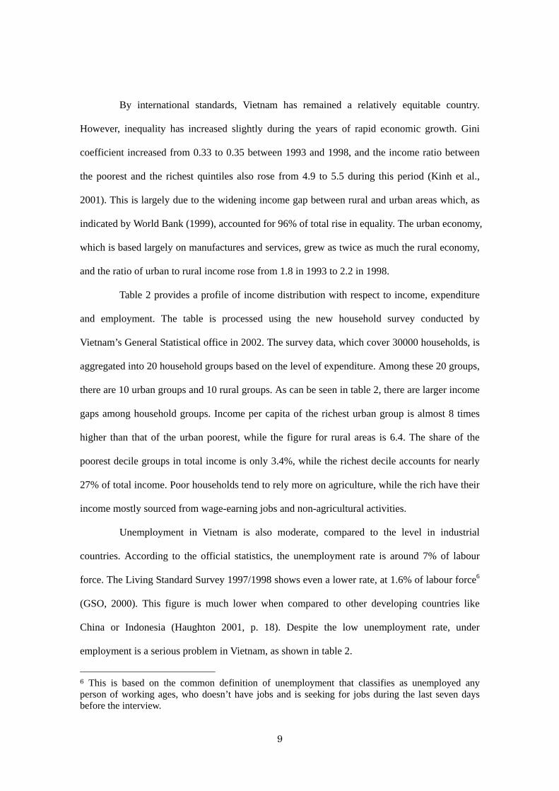
By international standards, Vietnam has remained a relatively equitable country.

However, inequality has increased slightly during the years of rapid economic growth. Gini

coefficient increased from 0.33 to 0.35 between 1993 and 1998, and the income ratio between

the poorest and the richest quintiles also rose from 4.9 to 5.5 during this period (Kinh et al.,

2001). This is largely due to the widening income gap between rural and urban areas which, as

indicated by World Bank (1999), accounted for 96% of total rise in equality. The urban economy,

which is based largely on manufactures and services, grew as twice as much the rural economy,

and the ratio of urban to rural income rose from 1.8 in 1993 to 2.2 in 1998.

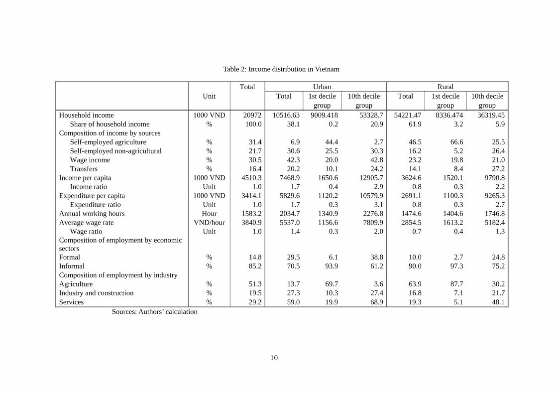
Table 2 provides a profile of income distribution with respect to income, expenditure

and employment. The table is processed using the new household survey conducted by

Vietnam’s General Statistical office in 2002. The survey data, which cover 30000 households, is

aggregated into 20 household groups based on the level of expenditure. Among these 20 groups,

there are 10 urban groups and 10 rural groups. As can be seen in table 2, there are larger income

gaps among household groups. Income per capita of the richest urban group is almost 8 times

higher than that of the urban poorest, while the figure for rural areas is 6.4. The share of the

poorest decile groups in total income is only 3.4%, while the richest decile accounts for nearly

27% of total income. Poor households tend to rely more on agriculture, while the rich have their

income mostly sourced from wage-earning jobs and non-agricultural activities.

Unemployment in Vietnam is also moderate, compared to the level in industrial

countries. According to the official statistics, the unemployment rate is around 7% of labour

force. The Living Standard Survey 1997/1998 shows even a lower rate, at 1.6% of labour force6

(GSO, 2000). This figure is much lower when compared to other developing countries like

China or Indonesia (Haughton 2001, p. 18). Despite the low unemployment rate, under

employment is a serious problem in Vietnam, as shown in table 2.

6 This is based on the common definition of unemployment that classifies as unemployed any person of working ages, who doesn’t have jobs and is seeking for jobs during the last seven days before the interview.

10

Table 2: Income distribution in Vietnam

Total Urban Rural Unit Total 1st decile 10th decile Total 1st decile 10th decile group group group group Household income 1000 VND 20972 10516.63 9009.418 53328.7 54221.47 8336.474 36319.45 Share of household income % 100.0 38.1 0.2 20.9 61.9 3.2 5.9 Composition of income by sources Self-employed agriculture % 31.4 6.9 44.4 2.7 46.5 66.6 25.5 Self-employed non-agricultural % 21.7 30.6 25.5 30.3 16.2 5.2 26.4 Wage income % 30.5 42.3 20.0 42.8 23.2 19.8 21.0 Transfers % 16.4 20.2 10.1 24.2 14.1 8.4 27.2 Income per capita 1000 VND 4510.3 7468.9 1650.6 12905.7 3624.6 1520.1 9790.8 Income ratio Unit 1.0 1.7 0.4 2.9 0.8 0.3 2.2 Expenditure per capita 1000 VND 3414.1 5829.6 1120.2 10579.9 2691.1 1100.3 9265.3 Expenditure ratio Unit 1.0 1.7 0.3 3.1 0.8 0.3 2.7 Annual working hours Hour 1583.2 2034.7 1340.9 2276.8 1474.6 1404.6 1746.8 Average wage rate VND/hour 3840.9 5537.0 1156.6 7809.9 2854.5 1613.2 5182.4 Wage ratio Unit 1.0 1.4 0.3 2.0 0.7 0.4 1.3 Composition of employment by economic sectors

Formal % 14.8 29.5 6.1 38.8 10.0 2.7 24.8 Informal % 85.2 70.5 93.9 61.2 90.0 97.3 75.2 Composition of employment by industry Agriculture % 51.3 13.7 69.7 3.6 63.9 87.7 30.2 Industry and construction % 19.5 27.3 10.3 27.4 16.8 7.1 21.7 Services % 29.2 59.0 19.9 68.9 19.3 5.1 48.1

Sources: Authors’ calculation

11

Based on the full-time annual work of 2000 hours, around 50% of urban workers and

70% of rural workers can be seen as underemployed7. On average, a Vietnamese worker works

only less than 1600 hours a year, suggesting an underemployment rate of more than 20%. The

incidence of underemployment varies across regions and household groups. Reflecting the

limited availability of arable land and off-farm jobs, underemployment is particularly high in

rural areas where an average worker uses only three-fourths of his working time. In urban areas,

underemployment is generally less serious, with the average year-round number of working

hours amounting to over 2000. However urban low-income groups have less working time than

high-income groups. A similar trend is also observed in rural areas, where underemployment

mainly affects low-income groups.

The difference in underemployment partly reflects the composition of jobs.

Low-income groups tend to involve mainly in agricultural activities, where production is subject

to seasonality and the availability of land. The urban lowest income group spends nearly 70% of

their working time on agriculture, while the figure for the rural lowest income group is 88%.

Low-income groups also involve more in trade and other low-productivity services in the

informal sector. By contrast, higher income groups tend to work more in industries and formal

services8. The average wage rates of poor groups are considerable low compared to high income

groups. For example, the average wage rate of the rural lowest income group is around 40% of

the national average wage, and the figure for the urban lowest income group is only 30%.

4. Model Specification

This section will discuss the major characteristics of the global CGE model used in

this paper. Our model generally follows the standard neoclassical CGE model (Dervis et al.,

7 This is calculated based on the assumption of full-time work of 40 hours per week and 50 working weeks a year. 8 The formal sector consists of the state sectors and foreign-invested sector, while the rest of the economy can be considered as informal.

12

1982), but extends the standard model by allowing for several countries and regions and

international link mechanisms.9 Specifically, our model specifies 10 industries and 11 countries

or regions. Ten industries consist of crops, other agricultural activities, mining, food processing,

light manufactures, heavy manufactures, machinery and equipment, public utilities, construction

and services. The specification of countries or regions in the model is chosen with the focus on

the East Asian region. Eleven countries and regions are China, Indonesia, Malaysia, Thailand,

Philippines, Vietnam, East Asian newly industrializing economies (NIEs), Japan, the North

American free trade area (NAFTA), the European Union (EU) and the rest of the world.

4.1. Country models

In country models, domestic output in each sector is a Constant Elasticity of

Substitution (CES) function between capital and labour. Domestic output is supplied to

domestic or foreign markets, depending on the prices in these markets. Domestic producers,

who seek to maximize profits, decide how much they sell in domestic and foreign markets. The

treatment of export supply is based on the Constant Elasticity of Transformation (CET) function.

The supply for domestic products and exports is derived from the revenue maximization

condition.

The factor demand is derived from the profit maximization condition, and factor

remuneration is equal to the value added price times the partial derivative of the production

function with respect to each factor. Capital is intersectorally immobile, and the capital stock in

each sector is fixed, letting the first-order condition to determine capital rents. The treatment of

the labour market assumes full employment and allows for labour mobility, but takes into

consideration distortions in the labour market. The model generally specifies two kinds of

labour, that is, skilled labour and unskilled labour. Sectoral labour demand is a CES function of

9 Our model of Vietnam and global link system originate from Nguyen (2003), Nguen (2002), Ezaki and Nguyen (2001), Ezaki (2001), Ezaki and Le (1997), etc.

13

skilled and unskilled labour, and the demand for each type of labour is derived from the

first-order condition. Sectoral wages are equal to the average wage level times fixed coefficients,

which represent wage differentials between economic sectors and types of labour.

In regards to Vietnam’s model, each type of labour is further divided into formal and

informal labour to capture the characteristic of the segmented labour market. Labour can move

between these two sectors, but the wage rates of formal and informal labour are subject to

different adjustment mechanisms. For workers in the formal sector, which consist of workers in

the state sector and foreign invested firms, the real wage rates are fixed by institutional factors.

However, the informal sector, inclusive of agriculture and non-agricultural small businesses, is

largely unregulated in Vietnam, and the informal wage rate is treated as flexible. The supply of

labour to the informal sector is determined as the difference between total supply of labour and

the demand for formal labour.

The model specifies two economic institutions, that is, household and government.

Household income consists of labour and capital income, which is allocated to each household

by using fixed coefficients. Government revenue consists of indirect taxes, import tariffs and

export duties. Savings by each institution are the difference between income and expenditure.

On the demand side, household consumption demand is based on a Cobb-Douglas utility

function, with fixed expenditure shares. Government demand for final goods is defined using

fixed expenditure shares of government real spending. The demand for inventory investment is

determined by using the fixed proportions of sectoral output. Total fixed investment is

determined by available savings, and the demand for capital goods is then computed through

exogenous coefficients.

Total domestic demand is satisfied through domestic production and imports. The

demand for imports is modeled using the Armington structure, in which domestic and foreign

goods are imperfect substitutes. The sectoral composite good, or total domestic demand, is a

CES function of imported and domestically produced goods, and the demand for imports is

14

derived from the cost minimization condition.

4.2. International linkages

Country models are linked through bilateral trade flows. Since the model allows for

different tariffs by countries of origin, the prices of imports varies with the import sources.

Specifically, the import price at the domestic market is equal to the export price of the country

of origin times the corresponding tariff rates. Domestic consumers and producers differentiate

imports by sources, that is, imports coming from different countries are considered as imperfect

substitutes. This characteristic is also modeled with the Armington structure. At the aggregate

level, total imports is a CES function of imports from different sources, and then the demand for

imports from each sources is derived from the cost minimization condition.

On the export side, exporters do not differentiate exports by countries of destination,

that is, commodities supplied to foreign countries are seen as perfectly homogenous and are sold

at the same price. The trade consistency is held so that total exports supplied by home countries

must be equal to the sum of imports by foreign countries. To put it more specifically, imports

from countries or regions must be summed up to total exports by that country or region. The

model does not allow for any movement of labour between countries or regions, that is, labour

is internationally immobile. Similarly, since foreign savings are fixed exogenously, capital is

also internationally immobile. Thus trade flows provide the only channel, by which any change

in economic policies or economic environment in one country transmit its effect to other

countries.

4.3. Equilibrium conditions

Equilibrium conditions consist of the conditions in factor, commodity and foreign

exchange markets. In the capital market, capital stocks are fixed and capital rents serve as

equilibrating variables. In the labour market, total supply of skilled and unskilled labour is held

15

fixed at the base-run level, and the labour market equilibrium determines wage rates. For

Vietnam’s model, there are two different equilibrating mechanisms for formal and informal

labour markets. In the formal sector, wage rates held fixed by institutional factors and the

equilibrium condition determines the demand for formal labour. In the informal labour market,

wage rates adjust flexibly to attain the equilibrium between supply and demand.

Equilibrium in product markets equates the supply of the composite good in each sector

to the sum of product demand with domestic prices serving as equilibrating variables. The fiscal

balance is implied in the treatment of the government sector, in which government consumption

and savings are fixed shares of government revenue. In the foreign exchange market, foreign

savings held fixed and equilibrium is achieved through price adjustments, i.e. the exchange rate

adjusts to balance the market supply of and the demand for foreign exchange. As for the

savings-investment identity, we adopt a so-called savings-driven closure, which requires that

total nominal investment is equal to total available savings.

Since CGE models determine only relative prices, it is necessary to select a numeraire

to define the absolute price level. For the country model, we fix the consumer price index and

leave the saving-investment balance as redundant. For the whole system, the exchange rate of

the North America is selected as the numeraire, i.e. all prices and nominal variables of the

model are defined in terms of the North American exchange rate or US dollars. It should be

noted that, since our model is homogenous in all prices, the selection of a numeraire is simply a

matter of convenience, and does not affect simulation results. The advantage of fixing the

consumer price index is that it allows the country model to determine all variables in real terms,

i.e. all variables are being deflated by appropriate price indices. The selection of the North

American exchange rate as the international numeraire is to conform with the common practice

in international trade, where the US dollar is most frequently used.

16

5. Simulation Analysis

5.1. Data and the Model calibration

To run the model, we make use of GTAP database version 6.0, which is constructed for 2001.

The GTAP database is a highly disaggregated global input-output table, differentiating 57

industries and 87 countries or regions. These data are then aggregated into 10 industries and 11

countries or regions in accordance with the model. We take 2001 as the benchmark year and use

GTAP data to calculate most of the parameters used in the model, such as consumption share,

saving rates, tax rates and wage rates. As for labour and capital, GTAP database provides only

information on total labour and capital stock for each country or region. Total labour and capital

stock is then allocated to each industry by assuming uniform wage rates and uniform capital

rents.

Data on tariffs and some non-tariff barriers is also available from GTAP database, and

is summarized in table 3. The upper part of table 3 shows tariff rates computed from GTAP data,

and the lower parts show data on export-tax equivalent rates of the Multi-fibre Agreement

(MFA). As can be seen in table 3, high tariffs are mainly imposed on crop products, processed

food and light manufactures. The data shows high average tariff rates for Vietnam, China and

Thailand, while average rates for other countries and regions are relatively low.

To calculate the share and scale parameters in trade and production functions, we

follow the common calibration procedure discussed in Shoven and Whalley (1984). The

elasticities of substitution in trade and production function are taken from GTAP database,

consisting of the elasticity of substitution between labour and capital, the elasticity of

substitution between domestically produced goods and imports and the elasticity of substitution

between imports from different sources. Generally GTAP database gives high values to the

elasticities in trade functions, while assigning relatively low values to the elasticity of

substitution in production functions. We assign a value of 1.2 to the elasticity of transformation

in the export supply function for all industries. Given the type of functions and the value of the

17

elasticities, the scale and share parameters can be calculated directly from the benchmark data.

As for Vietnam’s model, the household sector is constructed using Vietnam’ living

standard survey (VLSS) conducted by the General Statistical Office in 2002. As mentioned

above, 20 household groups are specified, consisting of 10 urban and 10 rural groups. From the

VLSS 2002, we calculate household income and expenditure, which are disaggregated for

around 70 industries. This information is used to allocate GTAP data on total income and

expenditure to each household group. Data on household employment is also derived from the

VLSS 2002, and is based on working hours instead of the number of workers10. This data is

computed for each type of jobs, i.e. formal and skilled workers, informal and skilled workers,

formal and unskilled workers and informal and unskilled workers, and is used to allocate GTAP

data on total employment to household groups.

10 Since each worker can have more than one job, using the number of working hours could reflect better the employment composition.

18

Table 3: The structure of protection

China Indonesia Malaysia Philippines Thailand Vietnam NIEs Japan NAFTA EU ROW Tariff rates (%)

Crops 68.52 1.72 28.86 6.00 16.13 12.68 78.42 30.12 3.24 4.09 11.35 Other Agricultural activities 3.54 2.09 0.40 2.90 6.46 3.23 3.02 2.41 0.99 0.95 5.90 Mining 0.37 0.36 1.13 3.05 0.20 3.33 2.62 0.02 0.04 0.00 2.62 Food Processing 18.26 9.08 10.13 11.09 39.10 43.66 12.36 31.36 6.01 4.85 18.98 Light manufactures 16.46 6.82 8.67 5.92 12.08 25.42 2.38 5.66 4.89 1.36 12.17 Heavy manufactures 11.20 4.70 6.63 4.33 10.42 6.84 2.95 0.93 1.77 0.58 6.63 Machinery 12.50 4.57 3.59 1.33 8.63 18.05 1.58 0.04 1.07 0.53 6.93 Utility 0.00 0.00 0.00 0.00 0.00 0.00 0.00 0.00 0.00 0.00 0.66 Construction 0.00 0.00 0.00 0.00 0.00 0.00 0.00 0.00 0.00 0.00 0.00 Services 0.00 0.00 0.00 0.00 0.00 0.00 0.00 0.00 0.00 0.00 0.00 Average tariff rate 11.70 3.60 4.63 2.77 8.88 10.23 3.41 4.13 1.77 0.81 6.90

MFA export-tax equivalent rates (%) Crops 0.00 0.00 0.00 0.00 0.00 0.00 0.00 0.00 0.00 0.00 0.00 Other Agricultural activities 0.00 0.00 0.00 0.00 0.00 0.00 0.00 0.00 0.00 0.00 0.00 Mining 0.00 0.00 0.00 0.00 0.00 0.00 0.00 0.00 0.00 0.00 0.00 Food Processing 0.00 0.00 0.00 0.00 0.00 0.00 0.00 0.00 0.00 0.00 0.00 Light manufactures 3.10 1.51 0.84 1.31 1.72 0.24 0.78 0.00 0.00 0.00 0.51 Heavy manufactures 0.00 0.00 0.00 0.00 0.00 0.00 0.00 0.00 0.00 0.00 0.00 Machinery 0.00 0.00 0.00 0.00 0.00 0.00 0.00 0.00 0.00 0.00 0.00 Utility 0.00 0.00 0.00 0.00 0.00 0.00 0.00 0.00 0.00 0.00 0.00 Construction 0.00 0.00 0.00 0.00 0.00 0.00 0.00 0.00 0.00 0.00 0.00 Services 0.00 0.00 0.00 0.00 0.00 0.00 0.00 0.00 0.00 0.00 0.00 Average MFA rate 1.24 0.49 0.07 0.17 0.31 0.10 0.10 0.00 0.00 0.00 0.08

Sources: GTAP database version 6.0

19

5.2. Simulation Results

The model described in section 4 is employed to analyze the effect on Vietnam of different

economic integration scenarios. Five simulations are performed and described briefly in table 4,

and simulation results are reported in tables 5 to 8. In all these simulation, we will focus on the

impact of tariff reductions and simply assume a complete removal of tariffs. This may be a

shortcoming as non-tariff barriers play an important role in protecting domestic industries in

many countries. However, data on non-tariff barriers are not available from GTAP database, and

it is difficult to collect this sort of data and quantify its tariff equivalent impacts.

Table 4: Simulation Scenarios

S0 Base run S1 Removing tariffs on the bilateral trade between Vietnam and ASEAN-4 S2 Removing tariffs on the bilateral trade between Vietnam, China and ASEAN-4 S3 Removing tariffs on the bilateral trade between Vietnam, China, ASEAN-4, East Asian

NIEs and Japan (East Asian Economic Ccommunity) S4 Removing tariffs on the bilateral trade between Vietnam, China, ASEAN-4, East Asian

NIEs, Japan and North America S5 Multilateral Trade liberalization

Simulation S1 is designed to evaluate the impacts of the ASEAN free trade area on

Vietnam. We remove all tariffs on the bilateral trade between Vietnam and four ASEAN

members, i.e. Indonesia, Thailand, Malaysia and Philippines11. The tariff removal stimulates the

bilateral trade between ASEAN countries, and both exports and imports increase in all countries.

The extent to which exports or imports increase, however, depends on the structure of protection

and the composition of trade in each countries. Since foreign savings are fixed in the model, the

exchange rate will adjust to attain the current account balance. The exchange rate depreciates if

imports increase more than exports and it appreciates otherwise. At the aggregate level, the

exchange rate depreciates in all ASEAN countries with the exception of Indonesia. GDP falls

slightly in Vietnam and Thailand in the real term, but increases in Malaysia and Philippines. The 11 Hereafter we will refer to these countries as ASEAN-4.

20

increase in imports put a downward pressure on domestic demand and force domestic prices to

fall. Combined with the increase in income, this leads to an increase in consumption. The gain

in consumption can be seen in all countries, with the biggest gain is observed in Malaysia.

In regards to Vietnam, household income and consumption rise by around 1.7% on

average. All income groups have income gains, with the poor groups having slightly higher

gains than the rich. This is largely thanks to the increase in income to unskilled labour, which

constitute a large share in poor households’ income. The tariff removal in ASEAN trading

partners helps expand agriculture and labour-intensive industries, and generally have positive

effects on poverty reductions and income distribution in Vietnam. However, the AFTA tariff

removal also causes trade diversions, although the extent of diversions is not large. Both exports

to and imports from ASEAN countries rise sharply, while trade with non-ASEAN countries or

regions falls.

The impact of the recently established China-ASEAN free trade area is considered in

simulation S2, in which tariffs on the bilateral trade between China, Vietnam and ASEAN-4 are

completely eliminated. Similar to S1, exports and imports rise in all countries, and all countries

experiences gains in consumption, with the biggest gains can be seen in Malaysia. The exchange

rate depreciation occurs in all countries, except for Indonesia and Malaysia. The inclusion of

China seems have a negative impact on Japan and East Asian NIEs, with the volume of trade

declines slightly in these countries.

For Vietnam, real GDP fall by 0.2% but the gain in consumption increases to more

than 4%. Again, all household groups have gains in income and consumption, but the poor has

bigger gains compared to the rich. The rural groups also benefit more than urban groups. The

establishment of a free trade area between China and ASEAN, however, causes a considerable

trade diversion to Vietnam. Imports from China and exports to China rise sharply at the expense

of trade with other regions. The biggest falls are seen in imports from Japan and East Asian

NIEs, which decline by 37% and 30% respectively from the base-run values. This shows a

21

strong competition between imports from China and imports from Japan and NIEs.

In simulation S3, we examine the effect of the possible formation of the East Asian

economic community. In this simulation, we remove all tariffs on the bilateral trade between

East Asian countries, including Japan and East Asian NIEs. The bilateral trade between East

Asian countries increases, and both exports and imports rise in all countries. The establishment

of the East Asian free trade area, however, causes a trade diversion to the EU and North

America, which see a slight decline in exports and imports. All countries experience a gain in

income and consumption, and real GDP increases with the exception of China and Vietnam.

Compared to simulation S2, the inclusion of Japan and East Asian NIEs significantly

increases the welfare gain for Vietnam. Despite a small drop in real GDP, household

consumption and income rise by 8.8% and 8.1% respectively. Income to unskilled labour rises

more than income to capital and skilled labour, and benefits mostly poor and rural household

groups. As for the trade direction, Vietnam’s trade is diverted from the US and the EU, which

see exports to Vietnam to fall by 16.5% and 21% respectively. Both exports and imports to East

Asian NIEs rise, while imports from Japan fall to a lesser extent compared to S2.

In simulation S4, we remove the tariffs on the bilateral trade between North America

and East Asian countries. This simulation is designed to evaluate the effect of the trade

liberalization under the APEC forum, which has set the objective of liberalizing trade and

investment regimes by the year 202012. Imports and exports increase in all APEC members but

at the expense of the EU and the rest of the World, and all APEC countries experience gains in

income and consumption. The removal of the NAFTA tariff also brings additional welfare gains

to Vietnam, where household income and consumption rise by 8.4% and 9.1% respectively. As

it may be expected, Vietnam’s trade is redirected toward APEC countries, and trade with the EU

and the rest of the world falls.

12 In this simulation, we assume tariffs are removed for only member countries. Indeed, as it is commonly believed, the APEC forum adopts the open regionalism, in which trade liberalization measures are applied to both member and non-member countries.

22

Finally, the effect of a multilateral liberalization is considered in simulation S5, in

which tariffs are completely eliminated for all countries and regions. Exports and imports rise,

with the total world exports increase by 3.4%. The welfare gain is also significant, with total

world consumption rise by 0.9%, or equivalent to $180 billions. The tariff removal on a

multilateral basis increases significantly the welfare gain for Vietnam, where household

consumption increases by 10.8% and exports increase by more than 20%. The multilateral trade

liberalization also reduces the extent of trade diversions caused by the regional integration as it

is seen in the previous simulations. The increase in Vietnam’s imports from ASEAN member

falls to only 1.7%, while imports from the EU and North America still decline but to a lesser

extent compared to S1 or S2.

We conclude the discussion in this section with some remarks on the implication for

foreign investment in Vietnam. Since the model focuses on the trade flows, foreign savings are

fixed and the changes in capital inflows or outflows are not taken into account. As can be seen

in table 6, capital rents for Vietnam increase in all simulations. Moreover, even it is not shown

in details, the increase in the capital rents of Vietnam is the highest as compared to other regions

or countries. The rising capital rent is obviously a good signal to foreign investors, who are

seeking for profits. This is to say that the regional integration and trade liberalization could

make investments in Vietnam become more profitable, and makes Vietnam become more

attractive to foreign investors.

23

Table 5: Effect of economic integration on countries or regions China Indonesia Malaysia Philippines Thailand Vietnam NIEs Japan NAFTA EU ROW Simulation Scenarios S1 Real GDP 0 0 0.03 0.01 -0.02 -0.07 0 0 0 0 0 Consumption -0.02 0.48 4.08 0.77 1.85 1.69 -0.05 -0.01 0 0 -0.01 Imports -0.08 1.78 2.12 1.24 2.34 1.86 -0.12 -0.13 -0.02 -0.01 -0.03 Exports -0.02 0.34 0.65 0.73 1.35 3.3 -0.04 -0.05 -0.01 0 -0.01 Simulation Scenarios S2 Real GDP 0 -0.01 0.06 0.02 -0.01 -0.18 0 0 0 0 0 Consumption 0.47 0.94 5.95 1.17 3.39 4.31 -0.22 -0.04 -0.01 -0.01 -0.02 Imports 1.67 3.67 4.23 1.92 5.16 5.27 -0.47 -0.49 -0.07 -0.04 -0.07 Exports 1.17 0.78 1.11 1.13 2.21 6.27 -0.13 -0.15 -0.02 -0.01 -0.03 Simulation Scenarios S3 Real GDP -0.19 0 0.11 0.05 -0.09 -0.42 0.06 0 0 0 0 Consumption 2.28 1.12 6.73 0.92 6.22 8.77 1.93 0.37 -0.04 -0.06 -0.06 Imports 8.93 3.24 4.23 1.2 8.91 11.82 3.02 3.63 -0.44 -0.19 -0.3 Exports 5.2 1.26 2.14 1.52 4.18 14.1 2.42 2.02 -0.12 -0.03 -0.12 Simulation Scenarios S4 Real GDP -0.2 -0.01 0.13 0.08 -0.1 -0.25 0 0 -0.01 0 -0.01 Consumption 3.42 1.39 7.76 1.18 6.46 9.12 2.8 0.7 0.2 -0.13 -0.13 Imports 12.11 4.89 5.22 1.64 9.13 12.67 4.38 5.42 1.45 -0.34 -0.53 Exports 6.9 1.17 2.28 1.98 4.56 15.82 3.12 3.47 1.94 -0.04 -0.32 Simulation Scenarios S5 Real GDP -0.5 -0.09 0.08 0.1 -0.33 -0.13 -0.01 -0.02 -0.01 0.04 0 Consumption 5.24 2.51 9.25 0.88 8.51 10.82 3.3 0.85 0.3 0.09 2.41 Imports 19.19 9.69 7.86 1.01 12.25 16.26 5.53 6.82 2.05 0.59 6.53 Exports 9.22 1.27 2.59 2.31 5.84 20.52 4.28 4.51 3.47 1 5.09

24

Table 6: Effect of trade liberalization on Vietnam Unit Base run Percentage change (%) S0 S1 S2 S3 S4 S5 GDP deflator Unit 1.00 1.74 4.27 8.6 8.85 10.61 Consumer price index Unit 1.00 0 0 0 0 0 Exchange rate Unit 1.00 0.84 1.22 3.96 3.24 1.47 Average wage rate Thousand USD 0.28 1.62 3.98 8.53 9.13 11.17 Skilled labor Thousand USD 0.55 1.45 3.5 7.77 8.51 10.19 Unskilled labor Thousand USD 0.21 1.87 4.54 9.33 9.75 12.08 Capital rent Unit 0.18 1.64 4.17 7.67 7.82 9.13 Real GDP Million USD 30751.82 -0.07 -0.18 -0.42 -0.25 -0.13 Output Million USD 66581.06 0.44 0.85 1.87 2.32 3.24 Private consumption Million USD 27213.03 1.69 4.31 8.77 9.12 10.82 Government consumption Million USD 2607.10 -12.99 -26.52 -43.96 -43.69 -44.09 Real investment Million USD 12939.39 -1.13 -0.8 -2.79 -3.43 -4.72 Imports Million USD 27434.46 1.86 5.27 11.82 12.67 16.26 Exports Million USD 15426.76 3.3 6.27 14.1 15.82 20.52 Household income Million USD 28114.30 1.67 4.15 8.09 8.41 10.03 Labor income Million USD 11590.04 0 0 0 0 0 Labor income (skilled labor) Million USD 4739.21 1.45 3.5 7.77 8.51 10.19 Labor income (unskilled labor) Million USD 6850.83 1.87 4.54 9.33 9.75 12.08 Capital income Million USD 16524.26 1.64 4.17 7.67 7.82 9.13

25

Table 7: Effect on income distribution of Vietnam Total household income Total household consumption S1 S2 S3 S4 S5 S1 S2 S3 S4 S5 Percentage change compared to the base run (%) Urban group 1 2 4.45 9.13 9.31 11.52 1.99 3.98 10.01 10.38 12.61 Urban group 2 1.85 4.55 9.61 10.01 12.57 1.87 4.12 10.51 11.06 13.66 Urban group 3 1.48 3.59 7.02 6.87 7.85 1.46 3.18 7.7 7.67 8.67 Urban group 4 1.42 3.5 7.75 8.03 9.78 1.35 2.97 8.04 8.42 10.17 Urban group 5 1.55 3.96 8.18 8.68 10.81 1.56 3.59 8.85 9.46 11.6 Urban group 6 1.45 3.95 7.49 7.89 9.55 1.36 3.48 7.57 8.03 9.7 Urban group 7 1.69 3.82 7.8 8.24 9.82 1.62 3.47 7.9 8.39 9.98 Urban group 8 1.46 3.96 8.32 8.92 10.84 1.31 3.53 7.96 8.58 10.5 Urban group 9 1.48 3.54 7.63 8.23 9.89 1.36 3.3 7.43 8.03 9.73 Urban group 10 1.32 3.38 7.27 7.79 9.14 1.31 3.64 7.57 8.09 9.53 Rural group 1 2.48 5.54 9.27 8.79 10.24 2.53 5.22 10.71 10.43 11.95 Rural group 2 2.31 5.28 9.18 8.91 10.59 2.35 4.94 10.4 10.3 12.02 Rural group 3 2.11 5.02 9.01 8.89 10.63 2.15 4.7 10.13 10.16 11.94 Rural group 4 2.14 5.1 9.4 9.49 11.69 2.14 4.75 10.22 10.43 12.67 Rural group 5 1.98 4.91 8.77 8.79 10.52 1.97 4.61 9.48 9.59 11.36 Rural group 6 2.01 5.02 9.17 9.29 11.17 2.02 4.84 9.88 10.08 12.01 Rural group 7 1.82 4.49 8.36 8.53 10.23 1.86 4.53 9.14 9.37 11.14 Rural group 8 1.8 4.58 8.6 8.84 10.57 1.87 4.9 9.49 9.77 11.6 Rural group 9 1.67 4.32 8.25 8.61 10.26 1.79 5.06 9.29 9.66 11.44 Rural group 10 1.43 3.66 7.16 7.54 8.95 1.83 5.76 9.62 9.96 11.63

26

Table 8: Effect on the trade direction of Vietnam Imports Exports S1 S2 S3 S4 S5 S1 S2 S3 S4 S5 China -12.95 174.17 101.43 97.73 89.69 -4.41 158.32 132.81 103.91 72.52 Indonesia 130.33 75.88 21.13 17.54 3.60 24.67 16.91 13.80 24.11 31.13 Malaysia 90.88 45.23 3.71 3.18 -5.65 9.22 -7.60 -11.02 -12.53 -17.05 Philippines 110.29 78.95 13.62 9.45 7.96 112.17 103.90 90.69 95.15 89.36 Thailand 140.10 43.44 8.01 8.60 5.56 176.03 157.65 124.32 120.76 92.93 NIES -13.18 -29.77 30.20 30.00 27.29 -4.87 -10.51 22.91 20.34 5.60 Japan -14.63 -36.87 -12.87 -11.68 -11.96 -6.37 -9.47 15.52 9.08 -2.47 NAFTA -3.06 -6.25 -8.94 -2.11 1.68 -6.98 -10.59 -11.27 33.20 20.50 EU -5.33 -11.94 -16.51 -15.64 -3.28 -0.69 -3.46 1.96 -0.45 27.23 Rest of the World -6.63 -11.51 -21.01 -20.73 -5.07 -4.59 -9.57 -8.34 -6.47 8.87 ASEAN-4 121.28 51.12 9.14 8.44 1.70 99.29 85.70 69.33 70.30 58.92 ASEAN-4 plus China 52.69 114.00 56.30 54.06 46.66 58.86 114.01 94.08 83.40 64.22 East Asia 9.78 19.64 31.71 31.05 27.12 12.47 25.12 39.78 33.22 18.62 Total 2.55 5.04 8.64 9.35 12.73 3.30 6.27 14.10 15.82 20.52

27

6. Summary and Conclusions

In this paper, we have constructed a global CGE model, which specifies 10 industries and 11

countries or regions. We have employed the model to examine the impact of the regional

economic integration on Vietnam’s economy, focussing on growth, poverty reductions and

income distribution. Five simulation scenarios have been carried out to analyze different

economic integration options facing Vietnam, including the ASEAN free trade area, the

China-ASEAN free trade area, the possible formation of an East Asian economic community,

APEC trade liberalization and the world-wide multilateral trade liberalization.

As discussed in the previous section, the impact of the trade liberalization and regional

economic integration on Vietnam’s economy is generally positive. The regional integration is

both welfare enhancing and income-distribution improving for Vietnam. Household

consumption and income rise significantly, and the poor and rural groups benefit more than the

rich. Moreover, the removal of tariffs in trading partners provides Vietnam with a greater market

access, and exports rise in all simulations. In terms of growth, trade liberalization may cause

real GDP to fall largely due to the sharp decrease in tariff revenue, but the overall output loss is

small.

From the above discussion, it is obviously desirable for Vietnam to actively participate

in the ongoing regional integration, including the ASEAN free trade area and the recently

established China-ASEAN free trade area. However, Vietnam should not confine itself to these

trading blocs. As shown in the simulation results, the gain from these trade areas is limited, and

the welfare gain for Vietnam could increase significantly when trade liberalization is carried out

on a broader basis, involving Vietnam’s major export markets such as Japan, the United States

or the European Union. The multilateral trade liberalization also reduces the extent of possible

trade diversions and further increases the market access for Vietnam’s exports.

28

References

Centre for International Economics (CIE), 1998, Trade Policies in Vietnam 1998, Canberra and

Sydney.

Centre for International Economics (CIE), 1999a, Trade and Industry Policies for Economic

Integration, Report prepared for CIEM and UNIDO, Canberra and Sydney.

Centre for International Economics (CIE), 1999b. Non-tariff Barriers in Vietnam: a framework

for developing a phase out strategy, Canberra and Sydney.

Dervis, K., J. de Melo, and S. Robinson, 1982, General Equilibrium Models for Development

Policies. A World Bank Research Publication, Cambridge University Press.

Ezaki, M. and Le Anh Son, 1997, “Prospects of the Vietnamese Economy in the Medium and Long

Run – A Dynamic CGE Analysis”, APEC Discussion Paper Series No.10, APEC Study Center,

Nagoya University and Institute of Developing Economies.

Ezaki, M., 2001, “Asian Economy in Future: An Econometric Analysis of Growth Perspectives,” in

Watanabe, T. (ed.), Economic Achievement in Asia, Tokyo: Toyo-Keizai (in Japanese).

Ezaki, M., and Nguyen Tien Dung, 2001, “Medium-Run Prospects of Viet Nam’s Economy: CGE

Simulation Analysis of the 7th Five-Year Plan,” Ministry of Planning and Investment (The

Socialist Republic of Viet Nam) and Japan International Cooperation Agency, Study on the

Economic Development Policy in the Transition toward a Market-Oriented Economy in the

Socialist Republic of Viet Nam (Phase 3), Final Report, Vol.1 General Commentary, Ch.4.

Forster, Neal, 1998, Vietnam’s Integration with ASEAN: a Policy Reader, United Nations

Development Program, Project VIE 95/015, Hanoi.

Fukase, Emiko and Will Martin, 1998, A Quantitative Evaluation of Vietnam’s Accession to the

ASEAN Free Trade Area (AFTA). Development Research Group, World Bank,

Washington DC.

Fukase Emiko and Will Martin, 1999, The effect of the United States’ Granting Most Favored

29

Nation Status to Vietnam. Development Research Group, World Bank, Washington DC.

General Statistical Office (GSO), 2000, Vietnam Living Standards Survey 1997-1998, Statistical

Publishing House, Hanoi.

General Statistical Office (GSO), 2003, Vietnam Living Standards Survey 2001-2002, Statistical

Publishing House, Hanoi.

General Statistical Offices (GSO), 2004, Statistical Yearbook 2003, Statistical Publishing House,

Hanoi.

Haughton, Dominique, Jonathan Haughton and Nguyen Phong, 2001, Living Standards during

an Economic Boom, Statistical Publishing House, Hanoi.

Haughton, Jonathan, 2001, “Introduction: Extraordinary Changes,” in Haughton et al. (2001).

Kinh Do Thien, Le Do Manh, Lo Thi Duc, Nguyen Ngoc Mai, Tran Quang, and Bui Xuan Du,

2001, “Inequality,” in Haughton et al. (2001).

Hertel, Thomas W. (ed.), 1997, Global Trade Analysis: Modeling and Applications, Cambridge

University Press.

Mansur, Ahsan and John Whalley, 1984, “Numerical Specification of Applied General

Equilibrium Models: Estimation, Calibration and Data,” in Scarf, H. E. and J. B. Shoven,

Applied General Equilibrium Analysis. Cambridge University Press.

McCarty, Adam, 1999, Vietnam’s Integration with ASEAN: Survey of Non-Tariff Measures

Affecting Trade, A report prepared for the Office of the Government of Vietnam, United

Nations Development Program, Project VIE 95/015, Hanoi.

Nguyen, Tien Dung, 2002, “Trade Reform in Vietnam: a CGE Analysis,” Forum of

International Development Studies, No.21.

Nguyen, Tien Dung, 2003, “Structural Adjustment in Vietnam: A Financial CGE Analysis,”

unpublished Ph.D. dissertation, Graduate School of International Development, Nagoya

University.

Robinson, S., 1989, “Multisectoral Models,” in Chenery, H. and T. N. Srinivasan (eds.),

30

Handbook of Development Economics. Elsevier Science Publishers.

Socialist Republic of Vietnam (SRV), 1999, “Individual Action Plan, 1999,” The document

submitted to the APEC Secretariats. APEC homepage: http.www.apecsec.org

Thang, Nguyen Xuan, 1999, Khu vuc mau dich tu do ASEAN va tien trinh hoi nhap cua Vietnam

(ASEAN free trade area and Vietnam’s integration), Statistical Publishing House, Hanoi

(in Vietnamese).

Tongzon, Jose L., 1999, “The Challenge of Regional Economic Integration: The Vietnamese

Perspective,” The Developing Economies, Vol.37, No. 2.

World Bank, 1999, Vietnam Development Report 2000: Attacking Poverty, Report No.

19914-VN, World Bank, Washington DC.

31

Appendix A: Global Linked CGE Model

A1. Equations of the Model Price Relations

(1) irkPMS = irkPM $ × rER × (1+ irktm )

(2) iririririr

irkir k irkSSir PMSaPM θθθθθω /)1()1/()1/(11 )( +++− ∑=

where ∑= k irkirkirir PMSMSPMM

(3) irPE = irPE$ × rER / (1+ irte )

(4) )1/(11 ( ir

irir MMir aP δω +−= iririririr

ir

irir

irMir PDPM δδδδδδδ ω /)1()1/()1/(1)1/( ))1( ++++−+

where iriririririr DPDMPMQP +=

(5) )1/(11 ( ir

irir EEir aPX γω −−= iririririr

ir

iririrEir PDPE γγγγγγγ ω /)1()1/()1/(1)1/( ))1( −−−− −+

where iriririririr DPDEPEXPX +=

(6) irPN = irPX - ∑ ×i irir Piocf - irPX × irtind

(7) rPINDEX = ∑i ircpcf × irP

Production functions (for competitive sectors)

(8) SirX =

irXa (irXω irp

irL− + (1- irXω ) irp

irK − ) irρ/1−

(9) SirD =

irEa )1/( irir γγ − )1((irEω− irPX / irPD ) )1/(1 irγ− × S

irX

where irir

ir

ir

irir irEirEEir DEaX γγγ ωω /1))1(( −+= ,

(10) irE = irEa )1/( irir γγ − (

irEω × irPX / irPE ) )1/(1 irγ− × SirX ,

32

Factor markets

(11) irL = irXa )1/( irir ρρ +− (

irXω irPN / irW ) )1/(1 irρ+ × SirX

(12) lirLK = irLa )1/( lirir λλ +− (

lirLω irW / lirWK ) )1/(1 irλ+ × irL

where irir

lirir l lirLLir LKaL λλω /1)( −−∑=

(13) iririririir

lirir l lirLLir WKaW λλλλλω /)1()1/()1/(11 )( +++− ∑=

where ∑= l lirliririr LKWKLW

(14) lirWK = lirwagcf ElrW , here lirwagcf = constant

(15) irK = irXa )1/( irir ρρ +− ((1-

irXω ) irPN / irR ) )1/(1 irρ+ SirX

Income and saving

(16) rYH = ( iri ir RK ×∑ + iri ir WL ×∑ )

for Vietnamr ≠

(17) hrYH = ( iriri hir KRykcf ××∑ + iriri hir LWylcf ××∑ )

for Vietnamr =

(18) rYG = ( rirkik irk ERPMMS ××∑ $ )× irktm +

iriri ir tindPXX ××∑ +

iriri ir tePEE ××∑

(19) rSH = rP YHsr×

for Vietnamr ≠

(20) rSH = ∑ ×h hrP YHs

hr

for Vietnamr =

(21) rSG = rG YGsr×

(22) rS = rSH + rSG

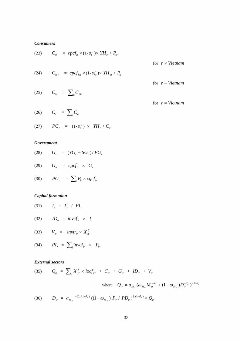
33

Consumers

(23) irC = ircpcf × (1- prs )× rYH / irP

for Vietnamr ≠

(24) hirC = hircpcf × (1- phrs )× hrYH / irP

for Vietnamr =

(25) irC = ∑h hirC

for Vietnamr =

(26) rC = ∑i irC

(27) rPC = (1- prs ) × rYH / rC

Government

(28) rG = rrr PGSGYG /)( −

(29) irG = ircgcf × rG

(30) rPG = iri ir cgcfP ×∑

Capital formation

(31) rI = nrI / rPI

(32) irID = irinvcf × rI

(33) irV = irinvtr × SirX

(34) rPI = ∑i irinvcf × irP

External sectors

(35) irQ = ∑ jSjrX × ijriocf + irC + irG + irID + irV

where irir

ir

ir

irir irMirMMir DMaQ δδδ ωω /1))1(( −−− −+=

(36) irD = irMa )1/( irir δδ +− )1((

irMω− irP / irPD ) )1/(1 irδ+ × irQ

34

(37) irM = irMa )1/( irir δδ +−

irMω( irP / irPM ) )1/(1 irδ+ × irQ

(38) rF$ = rF$

Linkage between Countries or Regions

(39). irk

irir

ir SSirk aMS ωθθ ()1/( +−= iririrk MPMPMS ir )1/(1)/ θ+

where irir

irkir l irkSSir MSaM θθω /1)( −−∑=

(40) ∑= k ikrSir MSE

(41) ikirk PEPM $$ =

(42) ∑ =r rF 0$

Equilibrium conditions

(43) irK = SirK

(44) liriKL∑ = S

lrL

(45) SirD = irD

(46) 0$$$ =−−∑∑ ri iririrkik irk FPEEPMMS

Walras’ law

(47) ∑ ∑ −×+−×i i

Srirr

Slrlir

Elr KKRLLKW )()( + )(∑ −

i irsirir DDPD +

−−+ nrrr IFS( )∑i irirVP + rER 0)$$$( =−−∑∑ ri iririrkik irk FPEEPMMS

(48) ∑ ∑∑ =−−r ri iririrkik irk FPEEPMMS 0)$$$(

35

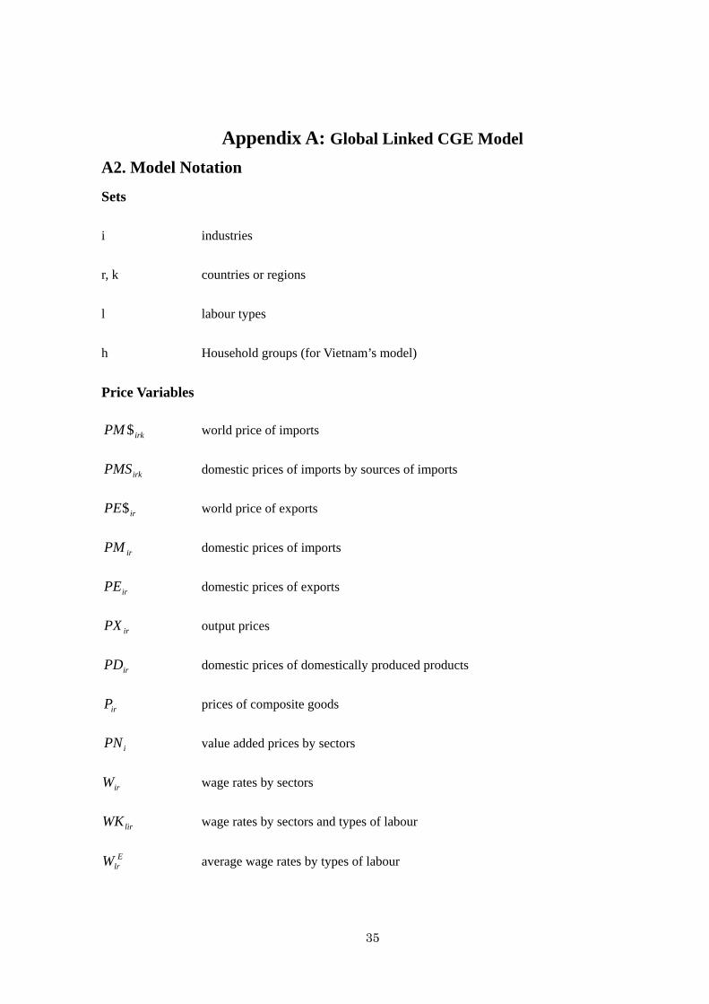
Appendix A: Global Linked CGE Model

A2. Model Notation

Sets

i industries

r, k countries or regions

l labour types

h Household groups (for Vietnam’s model)

Price Variables

irkPM $ world price of imports

irkPMS domestic prices of imports by sources of imports

irPE$ world price of exports

irPM domestic prices of imports

irPE domestic prices of exports

irPX output prices

irPD domestic prices of domestically produced products

irP prices of composite goods

iPN value added prices by sectors

irW wage rates by sectors

lirWK wage rates by sectors and types of labour

ElrW average wage rates by types of labour

36

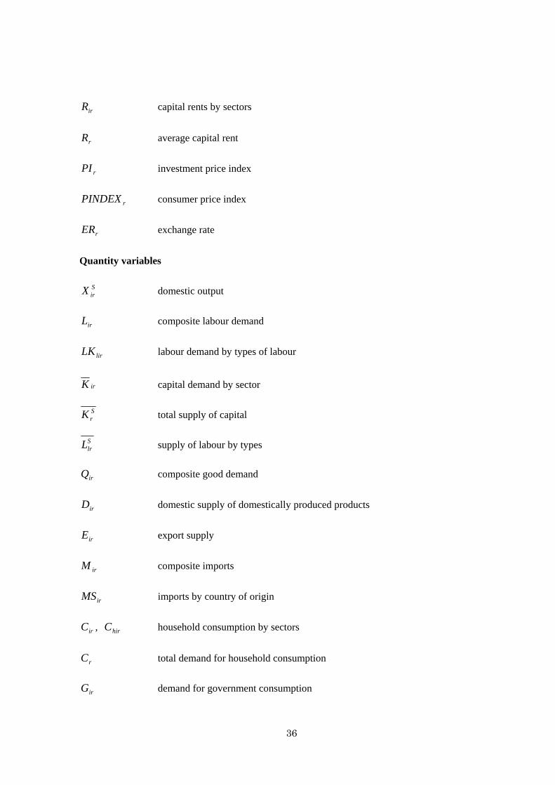
irR capital rents by sectors

rR average capital rent

rPI investment price index

rPINDEX consumer price index

rER exchange rate

Quantity variables

SirX domestic output

irL composite labour demand

lirLK labour demand by types of labour

irK capital demand by sector

SrK total supply of capital

SlrL supply of labour by types

irQ composite good demand

irD domestic supply of domestically produced products

irE export supply

irM composite imports

irMS imports by country of origin

irC , hirC household consumption by sectors

rC total demand for household consumption

irG demand for government consumption

37

rG total demand for government consumption

rF$ foreign savings

rI total real fixed investment

irID demand for capital goods

irV demand for inventory investment

rDEP total depreciation expenditure

Nominal variables

rYH , hrYH household income

rYG government revenue

rSH household savings

rSG government savings

rS domestic savings

nrI nominal fixed investment

Parameters

irXa scale parameters in production functions

irXω share parameters in production functions

irρ exponent parameters in production functions

irLa scale parameters in labour demand functions

lirLω share parameters in labour demand functions

irλ exponents in labour demand functions

38

irMa scale parameters in composite goods functions

irMω share parameters in composite goods functions

irδ exponents in composite goods functions

irSa scale parameters in import demand functions

irkSω share parameters in import demand functions

irθ exponents in import demand functions

irEa scale parameters in export supply functions

irEω share parameters in export supply functions

irγ exponents in export supply functions

ijriocf intermediate input coefficient of good j in industry i

ircpcf , hircpcf household consumption shares

ircgcf government consumption shares

irinvcf fixed investment shares

irinvtr ratios of inventory investment to real production

rPs ,hrPs household saving rates

rGs government saving rates

irtm import tariff rates

irte export duty rates

irtind indirect tax rates

39

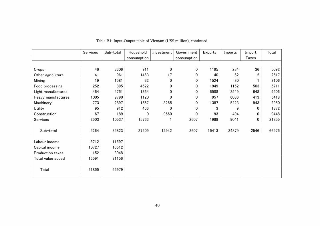
Appendix B: A Social Accounting Matrix for Vietnam

Table B1: Input-Output table of Vietnam (US$ million)

Crops Other agri- Mining Food pro- Light ma- Heavy ma- Machi- Utility Constru-

culture cessing nufactures nufactures nery ction

Crops 299 223 0 2600 116 20 0 0 2

Other agriculture 7 154 6 372 226 141 1 0 13

Mining 1 3 107 1 11 460 1 90 888

Food processing 6 150 0 480 4 3 0 0 0

Light manufactures 20 18 72 83 3321 312 71 45 345

Heavy manufactures 928 113 344 299 1114 1434 596 187 3770

Machinery 54 53 123 20 142 117 853 248 514

Utility 35 8 15 48 125 159 42 264 121

Construction 6 0 14 2 10 11 2 13 64

Services 692 285 1185 740 1780 1579 937 37 799

Sub-total 2047 1007 1867 4647 6850 4236 2505 885 6515

Labour income 1173 514 129 473 899 447 258 341 1651

Capital income 1621 894 800 299 423 510 110 119 1009

Production taxes 251 103 310 292 1334 225 77 27 273

Total value added 3045 1511 1239 1064 2656 1182 445 487 2933

Total 5092 2518 3106 5711 9506 5418 2950 1372 9448

40

Table B1: Input-Output table of Vietnam (US$ million), continued

Services Sub-total Household Investment Government Exports Imports Import Total

consumption consumption Taxes

Crops 46 3306 911 0 0 1195 284 36 5092

Other agriculture 41 961 1463 17 0 140 62 2 2517

Mining 19 1581 32 0 0 1524 30 1 3106

Food processing 252 895 4522 0 0 1949 1152 503 5711

Light manufactures 464 4751 1364 0 0 6588 2549 648 9506

Heavy manufactures 1005 9790 1120 0 0 957 6036 413 5418

Machinery 773 2897 1567 3265 0 1387 5223 943 2950

Utility 95 912 466 0 0 3 9 0 1372

Construction 67 189 0 9660 0 93 494 0 9448

Services 2503 10537 15763 1 2607 1988 9041 0 21855

Sub-total 5264 35823 27209 12942 2607 15413 24879 2546 66975

Labour income 5712 11597

Capital income 10727 16512

Production taxes 152 3048

Total value added 16591 31156

Total 21855 66979

41

Table B2: Income to formal and skilled labour (US$ million) Crops Other agri- Mining Food pro- Light ma- Heavy ma- Machi- Utility Constru- Services Total culture cessing nufactures nufactures nery ction Urban group 1 0.0 0.1 0.0 0.0 0.0 0.2 0.0 0.0 0.0 0.0 0.3 Urban group 2 0.0 0.0 0.0 0.2 0.1 0.0 0.0 0.0 0.0 0.6 0.9 Urban group 3 0.0 0.0 0.0 0.1 0.0 0.0 0.0 0.0 0.3 1.5 2.0 Urban group 4 0.0 0.0 0.6 0.2 1.4 1.3 0.0 0.0 0.0 4.4 7.8 Urban group 5 0.0 1.8 0.8 0.1 3.7 0.7 2.1 2.0 0.8 18.6 30.6 Urban group 6 0.9 0.0 2.1 4.0 2.6 3.4 0.0 11.6 8.0 29.7 62.4 Urban group 7 0.2 9.2 4.3 5.5 8.3 2.0 7.2 13.5 6.3 61.5 118.2 Urban group 8 4.2 7.0 12.2 13.1 15.9 12.1 11.8 24.7 23.6 102.8 227.5 Urban group 9 6.4 19.9 19.0 25.3 39.0 14.7 26.2 41.8 74.2 253.9 520.4 Urban group 10 11.7 53.6 34.5 94.6 122.2 59.4 49.4 95.0 290.9 820.5 1631.8 Rural group 1 1.8 0.0 0.0 1.8 0.7 0.0 0.0 0.0 2.6 4.1 11.0 Rural group 2 1.3 0.5 0.0 0.5 3.1 0.6 0.0 0.5 0.0 7.5 14.1 Rural group 3 1.0 0.0 0.4 0.8 2.3 0.0 0.3 0.0 0.0 23.2 28.1 Rural group 4 4.5 6.0 0.2 0.0 3.3 1.2 2.2 0.0 2.2 22.1 41.7 Rural group 5 4.8 5.8 0.0 0.0 4.7 4.4 2.7 1.5 4.5 40.4 68.7 Rural group 6 2.2 1.1 1.9 3.0 3.7 3.5 1.0 2.8 10.4 75.9 105.6 Rural group 7 6.4 0.0 0.7 5.1 17.0 9.3 0.4 4.9 6.1 115.0 165.0 Rural group 8 5.3 4.9 1.2 3.8 8.7 9.4 5.1 6.5 9.9 130.3 185.3 Rural group 9 9.3 2.1 3.7 12.5 7.9 14.1 16.5 35.7 11.0 141.0 253.8 Rural group 10 5.0 0.0 1.1 10.9 5.8 16.8 3.7 3.9 6.3 122.1 175.6 Total 65.2 112.0 82.9 181.6 250.6 152.8 128.8 244.5 457.1 1975.2 3650.8

42

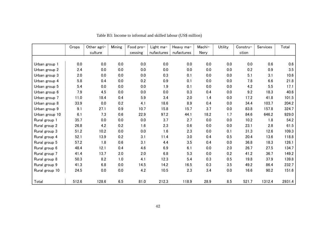
Table B3: Income to informal and skilled labour (US$ million)

Crops Other agri- Mining Food pro- Light ma- Heavy ma- Machi- Utility Constru- Services Total

culture cessing nufactures nufactures Nery ction

Urban group 1 0.0 0.0 0.0 0.0 0.0 0.0 0.0 0.0 0.0 0.6 0.6

Urban group 2 2.4 0.0 0.0 0.0 0.0 0.0 0.0 0.0 0.2 0.9 3.5

Urban group 3 2.0 0.0 0.0 0.0 0.3 0.1 0.0 0.0 5.1 3.1 10.6

Urban group 4 5.8 0.4 0.0 0.2 0.9 0.1 0.0 0.0 7.8 6.6 21.8

Urban group 5 5.4 0.0 0.0 0.0 1.9 0.1 0.0 0.0 4.2 5.5 17.1

Urban group 6 7.9 4.5 0.0 0.0 0.0 0.3 0.4 0.0 9.2 18.3 40.6

Urban group 7 11.0 18.4 0.4 5.9 3.4 2.0 1.4 0.0 17.2 41.8 101.5

Urban group 8 33.9 0.0 0.2 4.1 18.6 8.9 0.4 0.0 34.4 103.7 204.2

Urban group 9 9.1 27.1 0.9 10.7 15.8 15.7 3.7 0.0 83.8 157.8 324.7

Urban group 10 6.1 7.3 0.6 22.9 97.2 44.1 18.2 1.7 84.6 646.2 929.0

Rural group 1 35.7 0.0 0.0 0.0 3.7 2.7 0.0 0.0 10.2 1.8 54.2

Rural group 2 26.8 4.2 0.2 1.6 2.3 0.6 0.0 0.0 23.1 2.8 61.5

Rural group 3 51.2 10.2 0.0 0.0 1.6 2.3 0.0 0.1 31.3 12.6 109.3

Rural group 4 52.1 13.9 0.2 3.1 11.4 3.0 0.4 0.5 20.4 13.6 118.8

Rural group 5 57.2 1.8 0.6 3.1 4.4 3.5 0.4 0.0 36.8 18.3 126.1

Rural group 6 48.4 12.1 0.4 4.6 6.9 6.1 0.0 2.0 26.7 27.5 134.7

Rural group 7 41.4 13.7 2.0 2.0 6.8 5.3 0.0 0.2 41.2 36.7 149.2

Rural group 8 50.3 8.2 1.0 4.1 12.3 5.4 0.3 0.5 19.8 37.9 139.8

Rural group 9 41.3 6.8 0.0 14.5 14.2 16.5 0.3 3.5 49.2 86.4 232.7

Rural group 10 24.5 0.0 0.0 4.2 10.5 2.3 3.4 0.0 16.6 90.2 151.6

Total 512.6 128.6 6.5 81.0 212.3 118.9 28.9 8.5 521.7 1312.4 2931.4

43

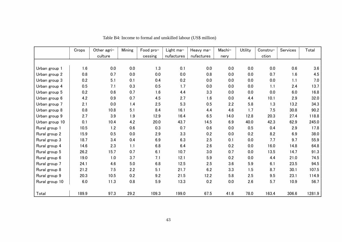
Table B4: Income to formal and unskilled labour (US$ million)

Crops Other agri- Mining Food pro- Light ma- Heavy ma- Machi- Utility Constru- Services Total

culture cessing nufactures nufactures nery ction

Urban group 1 1.6 0.0 0.0 1.3 0.1 0.0 0.0 0.0 0.0 0.6 3.6

Urban group 2 0.8 0.7 0.0 0.0 0.0 0.8 0.0 0.0 0.7 1.6 4.5

Urban group 3 0.2 5.1 0.1 0.4 0.2 0.0 0.0 0.0 0.0 1.1 7.0

Urban group 4 0.5 7.1 0.3 0.5 1.7 0.0 0.0 0.0 1.1 2.4 13.7

Urban group 5 0.2 0.6 0.7 1.6 4.4 3.3 0.0 0.0 0.0 6.0 16.8

Urban group 6 4.2 0.9 0.7 4.5 2.7 1.6 0.0 4.4 10.1 2.9 32.0

Urban group 7 2.1 0.0 1.4 2.5 5.3 0.5 2.2 5.8 1.3 13.2 34.3

Urban group 8 0.8 10.8 5.1 8.4 16.1 4.4 4.6 1.7 7.5 30.8 90.2

Urban group 9 2.7 3.9 1.9 12.9 16.4 6.5 14.0 12.8 20.3 27.4 118.8

Urban group 10 0.1 10.4 4.2 20.0 43.7 14.5 6.9 40.0 42.3 62.9 245.0

Rural group 1 10.5 1.2 0.6 0.3 0.7 0.6 0.0 0.5 0.4 2.9 17.8

Rural group 2 15.9 0.5 0.0 2.9 3.3 0.2 0.0 0.2 8.2 6.9 38.0

Rural group 3 18.7 3.4 0.4 6.9 6.3 2.5 0.1 0.0 7.7 9.7 55.9

Rural group 4 14.6 2.3 1.1 6.8 6.4 2.6 0.2 0.0 16.0 14.8 64.8

Rural group 5 26.2 15.7 0.7 6.1 10.7 3.0 0.7 0.0 13.5 14.7 91.3

Rural group 6 19.0 1.0 3.7 7.1 12.1 5.9 0.2 0.0 4.4 21.0 74.5

Rural group 7 24.1 4.6 5.0 6.8 12.5 2.5 3.6 5.9 6.1 23.5 94.5

Rural group 8 21.2 7.5 2.2 5.1 21.7 6.2 3.3 1.5 8.7 30.1 107.5

Rural group 9 20.3 10.5 0.2 9.2 21.5 12.2 5.8 2.5 9.5 23.1 114.9

Rural group 10 6.0 11.3 0.8 5.9 13.3 0.2 0.0 2.6 5.7 10.9 56.7

Total 189.9 97.3 29.2 109.3 199.0 67.5 41.6 78.0 163.4 306.6 1281.9

44

Table B5: Income to informal and unskilled labour (US$ million)

Crops Other agri- Mining Food pro- Light ma- Heavy ma- Machi- Utility Constru- Services Total

culture cessing nufactures nufactures nery ction

Urban group 1 0.0 0.0 0.0 0.0 0.0 0.0 0.0 0.0 0.0 1.7 1.7

Urban group 2 4.4 0.0 0.0 0.0 0.0 0.0 0.0 0.0 0.2 0.3 4.9

Urban group 3 2.0 0.0 0.0 0.0 0.5 0.1 0.0 0.0 2.2 0.2 5.0

Urban group 4 3.1 1.0 0.0 0.0 0.4 0.1 0.0 0.0 9.9 1.4 15.9

Urban group 5 3.6 0.0 0.0 0.0 1.3 0.1 0.0 0.0 4.7 3.2 12.9

Urban group 6 3.6 1.5 0.1 0.0 0.0 0.3 0.4 0.0 9.2 29.6 44.7

Urban group 7 4.8 21.6 0.1 5.4 2.8 1.4 2.2 0.0 17.4 37.0 92.5

Urban group 8 52.8 0.0 2.5 1.6 19.1 3.2 0.5 0.0 25.0 121.2 226.0

Urban group 9 1.3 50.5 0.9 15.2 20.8 18.4 1.1 0.0 86.3 262.2 456.7

Urban group 10 0.9 15.4 0.6 47.7 120.0 39.2 48.4 0.0 96.5 1159.6 1528.3

Rural group 1 22.5 0.0 0.0 0.0 6.4 3.3 0.0 0.0 9.2 2.7 44.1

Rural group 2 27.7 13.0 0.1 2.7 2.5 0.8 0.0 0.0 23.7 2.6 73.1

Rural group 3 50.3 7.2 0.0 0.0 2.6 1.4 0.0 0.1 27.5 16.5 105.6

Rural group 4 29.2 26.9 0.3 4.4 2.2 3.5 0.5 0.3 23.3 12.7 103.3

Rural group 5 38.5 0.3 0.6 1.5 4.1 3.2 0.5 0.0 35.3 19.3 103.3

Rural group 6 33.8 12.7 0.6 2.9 8.2 5.7 0.0 1.7 25.9 27.9 119.3

Rural group 7 25.7 17.7 2.5 1.9 10.2 4.9 0.0 0.2 36.6 55.0 154.6

Rural group 8 44.5 1.2 1.9 4.1 13.0 5.1 0.4 3.1 22.5 70.5 166.3

Rural group 9 52.2 7.1 0.0 12.6 9.3 15.4 0.4 4.6 33.9 131.4 266.9

Rural group 10 4.4 0.0 0.0 1.1 13.8 1.7 4.3 0.0 19.7 162.8 207.7

Total 405.3 176.1 10.3 101.1 237.2 107.7 58.7 10.0 508.8 2117.7 3732.9

45

Table B6: Total labour income (US$ million)

Crops Other agri- Mining Food pro- Light ma- Heavy ma- Machi- Utility Constru- Services Total

culture cessing nufactures Nufactures nery ction

Urban group 1 1.6 0.1 0.0 1.3 0.1 0.2 0.0 0.0 0.0 2.9 6.3

Urban group 2 7.7 0.7 0.0 0.2 0.1 0.8 0.0 0.0 1.1 3.3 13.8

Urban group 3 4.2 5.1 0.1 0.5 1.0 0.2 0.0 0.0 7.5 6.0 24.7

Urban group 4 9.3 8.5 0.9 1.0 4.4 1.5 0.0 0.0 18.8 14.7 59.2

Urban group 5 9.3 2.4 1.5 1.7 11.4 4.2 2.1 2.0 9.6 33.2 77.4

Urban group 6 16.6 7.0 2.9 8.5 5.3 5.7 0.7 16.1 36.5 80.5 179.6

Urban group 7 18.1 49.2 6.2 19.4 19.8 5.8 12.9 19.3 42.1 153.6 346.5

Urban group 8 91.8 17.8 20.1 27.2 69.6 28.6 17.3 26.4 90.5 358.5 747.9

Urban group 9 19.5 101.4 22.7 64.1 92.1 55.3 45.0 54.6 264.6 701.3 1420.6

Urban group 10 18.9 86.6 39.9 185.2 383.1 157.2 123.0 136.8 514.3 2689.2 4334.1

Rural group 1 70.6 1.2 0.6 2.1 11.4 6.6 0.0 0.5 22.5 11.6 127.0

Rural group 2 71.7 18.2 0.3 7.7 11.2 2.2 0.0 0.6 54.9 19.8 186.7

Rural group 3 121.2 20.8 0.8 7.7 12.8 6.2 0.4 0.2 66.5 62.1 298.8

Rural group 4 100.5 49.0 1.9 14.4 23.3 10.2 3.3 0.8 61.9 63.2 328.6

Rural group 5 126.7 23.5 2.0 10.7 23.8 14.1 4.2 1.5 90.1 92.8 389.4

Rural group 6 103.4 27.0 6.7 17.6 30.9 21.1 1.2 6.5 67.5 152.4 434.2

Rural group 7 97.7 35.9 10.3 15.8 46.5 22.0 4.0 11.1 89.9 230.2 563.3

Rural group 8 121.3 21.9 6.2 17.1 55.7 26.1 9.2 11.7 60.8 268.8 598.9

Rural group 9 123.1 26.5 3.9 48.8 52.9 58.1 23.1 46.4 103.6 381.9 868.3

Rural group 10 39.8 11.3 2.0 22.0 43.5 21.0 11.4 6.5 48.3 386.0 591.7

Total 1173.0 514.0 129.0 473.0 899.0 447.0 258.0 341.0 1651.0 5712.0 11597.0

46

Table B7: Total capital income (US$ million)

Crops Other agri- Mining Food pro- Light ma- Heavy ma- Machi- Utility Constru- Services Total

culture cessing nufactures Nufactures nery ction

Urban group 1 4.9 1.6 0.6 0.0 2.5 0.0 0.0 0.0 0.0 23.4 33.1

Urban group 2 2.8 1.5 7.4 0.3 0.3 0.0 5.9 0.0 2.1 32.5 52.8

Urban group 3 6.8 3.3 0.5 0.4 0.6 0.5 0.0 0.0 8.1 60.0 80.3

Urban group 4 7.2 4.2 1.2 0.8 1.8 0.1 0.0 0.0 0.0 84.4 99.5

Urban group 5 6.6 6.9 8.4 1.9 2.6 0.3 0.0 0.0 0.0 137.4 164.0

Urban group 6 15.5 9.3 26.1 2.8 4.4 3.5 4.0 21.1 1.7 267.9 356.2

Urban group 7 15.9 12.4 7.0 7.8 9.5 8.2 3.9 0.0 16.7 398.1 479.5

Urban group 8 15.5 11.2 21.4 7.8 14.5 35.3 2.1 3.3 116.8 703.4 931.3

Urban group 9 18.1 21.4 52.3 12.5 48.0 34.7 23.8 0.0 69.4 1213.4 1493.5

Urban group 10 14.3 27.1 35.8 75.4 106.2 168.4 53.7 1.6 464.0 3203.5 4150.0

Rural group 1 115.9 55.8 27.3 2.8 4.4 1.9 1.0 0.0 14.9 74.2 298.1

Rural group 2 141.6 69.7 35.7 10.8 12.0 7.0 0.0 6.0 5.4 173.5 461.7

Rural group 3 150.1 78.8 46.5 11.1 18.7 11.4 0.0 0.0 5.2 277.5 599.4

Rural group 4 169.4 85.4 73.0 16.2 24.1 14.7 0.9 0.0 34.6 298.8 717.2

Rural group 5 179.5 86.1 71.6 22.1 22.4 23.2 0.7 20.8 19.2 445.5 891.1

Rural group 6 189.0 95.0 60.8 20.6 34.1 51.3 4.0 5.3 24.9 500.2 985.1

Rural group 7 186.8 96.8 87.4 19.1 25.6 28.1 4.2 0.0 44.4 616.6 1109.0

Rural group 8 177.4 84.0 69.6 24.3 37.8 53.2 2.1 49.9 92.5 666.9 1257.6

Rural group 9 137.7 92.6 83.9 25.9 34.2 46.1 0.0 11.2 36.8 786.8 1255.3

Rural group 10 65.9 51.1 83.5 36.5 19.4 22.1 3.7 0.0 52.1 763.0 1097.4

Total 1621.0 894.0 800.0 299.0 423.0 510.0 110.0 119.0 1009.0 10727.0 16512.0

47

Table B7: Household expenditure (US$ million)

Crops Other agri- Mining Food pro- Light ma- Heavy ma- Machi- Utility Constru- Services Total

culture cessing Nufactures nufactures nery ction

Urban group 1 3.2 2.4 0.1 7.8 2.0 2.1 0.1 0.7 0.0 15.2 33.6

Urban group 2 3.4 3.5 0.1 11.2 3.1 3.0 0.2 1.0 0.0 23.9 49.3

Urban group 3 5.3 6.1 0.2 18.6 5.2 4.1 1.0 1.6 0.0 44.9 87.1

Urban group 4 6.7 9.0 0.3 25.9 6.8 6.6 1.2 2.3 0.0 70.1 128.8

Urban group 5 9.8 15.8 0.3 45.8 10.9 11.2 3.4 4.1 0.0 111.3 212.6

Urban group 6 15.6 25.3 0.6 70.9 20.5 18.0 6.7 8.1 0.0 229.2 394.8

Urban group 7 20.9 39.1 0.6 109.7 28.7 28.3 16.0 14.0 0.0 366.6 624.0

Urban group 8 30.3 67.7 0.7 179.8 46.6 47.8 32.5 26.9 0.0 733.9 1166.2

Urban group 9 47.7 113.1 0.8 331.9 92.0 82.6 89.1 51.5 0.0 1445.7 2254.4

Urban group 10 94.7 272.4 0.5 1011.1 292.8 243.6 509.8 152.2 0.0 4725.8 7302.8

Rural group 1 65.4 40.9 3.0 144.6 45.9 31.0 4.3 6.3 0.0 251.6 593.0

Rural group 2 74.3 65.8 3.3 204.8 64.6 48.4 8.1 9.6 0.0 399.6 878.6

Rural group 3 76.3 79.6 3.2 246.9 75.1 57.5 12.5 12.5 0.0 517.7 1081.3

Rural group 4 78.0 92.1 3.4 276.4 82.2 67.2 19.0 15.3 0.0 659.5 1293.0

Rural group 5 77.6 102.1 3.3 295.6 95.7 73.3 29.9 18.2 0.0 785.6 1481.3

Rural group 6 74.9 108.8 3.1 311.9 98.0 80.0 49.0 21.4 0.0 878.5 1625.9

Rural group 7 72.3 114.4 3.1 338.8 105.9 86.5 85.0 26.7 0.0 1039.1 1871.8

Rural group 8 67.4 116.0 2.6 343.4 104.4 85.3 138.1 30.5 0.0 1164.0 2051.7

Rural group 9 56.2 112.8 1.9 324.8 101.3 84.4 223.1 34.6 0.0 1313.2 2252.3

Rural group 10 30.9 76.0 0.8 222.2 82.6 59.3 337.8 28.4 0.0 987.5 1825.5

Total 911.0 1463.0 32.0 4522.0 1364.0 1120.0 1567.0 466.0 0.0 15763.0 27208.0

48

Appendix C: The Elasticities of Substitution

Table C1: The Elasticity of Substitution in Trade and Production Functions

Elasticity of substitution in

the production function Elasticity of substitution in

the composite goods function Elasticity of substitution in the import demand function

Crops 0.24 2.67 5.17 Other Agricultural activities 0.22 2.11 4.02 Mining 0.20 5.26 12.69 Food Processing 1.12 2.49 5.04 Light manufactures 1.26 3.46 7.20 Heavy manufactures 1.26 3.15 6.39 Machinery 1.26 3.84 7.83 Utility 1.26 2.80 5.60 Construction 1.40 1.90 3.80 Services 1.38 1.90 3.80