Discretization for naive-Bayes learning:

managing discretization bias and variance

Ying Yang Geoffrey I. Webb

School of Computer Science and Software EngineeringMonash University

Melbourne, VIC 3800, Australia

Abstract

Quantitative attributes are usually discretized in naive-Bayes learning. We provea theorem that explains why discretization can be effective for naive-Bayes learn-ing. The use of different discretization techniques can be expected to affect theclassification bias and variance of generated naive-Bayes classifiers, effects we namediscretization bias and variance. We argue that by properly managing discretiza-tion bias and variance, we can effectively reduce naive-Bayes classification error.In particular, we propose proportional k-interval discretization and equal size dis-cretization, two efficient heuristic discretization methods that are able to effectivelymanage discretization bias and variance by tuning discretized interval size and in-terval number. We empirically evaluate our new techniques against five key dis-cretization methods for naive-Bayes classifiers. The experimental results supportour theoretical arguments by showing that naive-Bayes classifiers trained on datadiscretized by our new methods are able to achieve lower classification error thanthose trained on data discretized by alternative discretization methods.

Key words: Discretization, Naive-Bayes Learning, Bias, Variance

1 Introduction

When classifying an instance, naive-Bayes classifiers assume attributes con-ditionally independent of each other given the class; and then apply Bayes’theorem to calculate the probability of each class given this instance. The classwith the highest probability is chosen as the class of this instance. Naive-Bayes

Email addresses: yyang@csse.monash.edu.au ( Ying Yang ),Geoff.Webb@csse.monash.edu.au ( Geoffrey I. Webb ).

1

classifiers are simple, effective, efficient, robust and support incremental train-ing. These merits have seen them deployed in numerous classification tasks.They have long been a core technique in information retrieval (Maron andKuhns, 1960; Maron, 1961; Lewis, 1992; Guthrie and Walker, 1994; Lewis andGale, 1994; Kalt, 1996; Larkey and Croft, 1996; Pazzani et al., 1996; Starret al., 1996a; Joachims, 1997; Koller and Sahami, 1997; Li and Yamanishi,1997; Mitchell, 1997; Pazzani and Billsus, 1997; Lewis, 1998; McCallum andNigam, 1998; McCallum et al., 1998; Nigam et al., 1998; Frasconi et al., 2001).They were first introduced into machine learning as a straw man against whichnew algorithms were compared and evaluated (Cestnik et al., 1987; Clark andNiblett, 1989; Cestnik, 1990). But it was soon realized that their classificationperformance was surprisingly good compared with other more sophisticatedclassification algorithms (Kononenko, 1990; Langley et al., 1992; Domingosand Pazzani, 1996, 1997; Zhang et al., 2000). Thus they have often been cho-sen as the base algorithm for bagging, boosting, wrapper, voting or hybridmethodologies (Kohavi, 1996; Zheng, 1998; Bauer and Kohavi, 1999; Tingand Zheng, 1999; Gama, 2000; Kim et al., 2000; Tsymbal et al., 2002). Inaddition, naive-Bayes classifiers also have widespread deployment in medicaldiagnosis (Kononenko, 1993; Kohavi et al., 1997; Kukar et al., 1997; McSherry,1997a,b; Zelic et al., 1997; Montani et al., 1998; Lavrac, 1998; Lavrac et al.,2000; Kononenko, 2001; Zupan et al., 2001), email filtering (Pantel and Lin,1998; Provost, 1999; Androutsopoulos et al., 2000; Rennie, 2000; Crawfordet al., 2002), and recommender systems (Starr et al., 1996b; Miyahara andPazzani, 2000; Mooney and Roy, 2000).

Classification tasks often involve quantitative attributes. For naive-Bayes clas-sifiers, quantitative attributes are usually processed by discretization, as theclassification performance tends to be better when quantitative attributes arediscretized than when their probabilities are estimated by making unsafe as-sumptions about the forms of the underlying distributions from which they aredrawn (Dougherty et al., 1995). Discretization creates a qualitative attributeX∗ from a quantitative attribute X. Each value of X∗ corresponds to an inter-val of values of X. X∗ is used instead of X for training a classifier. In contrastto parametric techniques for inference from quantitative attributes, such asprobability density estimation, discretization can avoid assuming quantitativeattributes’ underlying distributions. However, because qualitative data havea lower level of measurement than quantitative data (Samuels and Witmer,1999), discretization might suffer information loss. This information loss willaffect the learning bias and variance of generated naive-Bayes classifiers. Suchan effect is hereafter named discretization bias and variance. We believe thatanalysis of discretization bias and variance is illuminating. We investigate theimpact of discretization bias and variance on the classification performanceof naive-Bayes classifiers. The resulting insights motivate the development oftwo new heuristic discretization methods, proportional k-interval discretizationand equal size discretization. Our goals are to improve both the classification

2

efficacy and efficiency of naive-Bayes classifiers. These dual goals are of par-ticular significance given naive-Bayes classifiers’ widespread deployment, andin particular their deployment in time-sensitive interactive applications.

The rest of this paper is organized as follows. Section 2 presents an analysison discretization’s terminology and taxonomy. Section 3 defines naive-Bayesclassifiers. In naive-Bayes learning, estimating probabilities for qualitative at-tributes is different from that for quantitative attributes. Section 4 introducesdiscretization in naive-Bayes learning. It includes a proof that states particu-lar conditions under which discretization will result in naive-Bayes classifiersdelivering the same probability estimates as would be obtained if the correctprobability density function were employed. It analyzes the factors that mightaffect the discretization effectiveness in the multi-attribute learning context.It also proposes the bias-variance characteristic of discretization. Section 5provides a review of previous key discretization methods, discussing their be-haviors in terms of discretization bias and variance. Section 6 proposes two newheuristic discretization methods designed to manage discretization bias andvariance, proportional k-interval discretization and equal size discretization.Section 7 compares the algorithm computational time complexities. Section 8carries out experimental validation. Section 9 presents the conclusion.

2 Terminology and taxonomy

There is a large amount of literature addressing discretization, among whichthere is considerable variation in the terminology used to describe which typeof data is transformed to which type of data by discretization. There alsoexist various proposals to taxonomize discretization methods, each taxonomyemphasizing different aspects of the distinctions among the methods. Here weclarify the difference among these variations and choose terms for use hereafter.

2.1 Terminology

Discretization transforms one type of data into another type. The two datatypes are variously referred to in previous literature, as ‘quantitative’ vs.‘qualitative’, ‘continuous’ vs. ‘discrete’, ‘nominal’ vs. ‘ordinal’, or ‘categori-cal’ vs. ‘numeric’. Turning to the authority of introductory statistical text-books (Bluman, 1992; Samuels and Witmer, 1999), there are two parallelways to classify data into different types. Data can be classified into eitherqualitative or quantitative. Data can also be classified into different levels ofmeasurement scales.

3

Qualitative attributes, also often called categorical attributes, are attributesthat can be placed into distinct categories, according to some characteristics.Some can be arrayed in a meaningful rank order. But no arithmetic operationscan be applied to them. Examples are blood type of a person: A, B, AB, O ; andtenderness of beef: very tender, tender, slightly tough, tough. Quantitativeattributes are numerical in nature. They can be ranked in order. They alsocan be subjected to meaningful arithmetic operations. Quantitative attributescan be further classified into two groups, discrete or continuous. A discreteattribute assumes values that can be counted. The attribute can not assumeall values on the number line within its value range. An example is numberof children in a family. A continuous attribute can assume all values on thenumber line within the value range. The values are obtained by measuringrather than counting. An example is Fahrenheit temperature scale.

In addition to being classified as either qualitative or quantitative, attributescan also be classified by how they are categorized, counted or measured. Thistype of classification uses measurement scales, and four common types ofscales are used: nominal, ordinal, interval and ratio. The nominal level ofmeasurement classifies data into mutually exclusive (non overlapping), ex-haustive categories in which no order or ranking can be imposed on the data,such as blood type of a person. The ordinal level of measurement classifiesdata into categories that can be ranked; however, the differences between theranks can not be calculated meaningfully by arithmetic, such as tenderness ofbeef. The interval level of measurement ranks data, and the differences be-tween units of measure can be calculated meaningfully by arithmetic. However,zero in the interval level of measurement does not mean ‘nil’ or ‘nothing’, suchas Fahrenheit temperature scale. The ratio level of measurement possessesall the characteristics of interval measurement, and there exists a zero thatmeans ‘nil’ or ‘nothing’. In consequence, true ratios exist between differentunits of measure. An example is number of children in a family.

We believe that ‘discretization’ is best described as the conversion of quan-titative attributes to qualitative attributes. In consequence, we will addressattributes as either qualitative or quantitative throughout this paper.

2.2 Taxonomy

Discretization methods can be classified into either primary or composite.Primary methods accomplish discretization without referring to any otherdiscretization method. In contrast, composite methods are built on top of aprimary method.

Primary methods can be classified as per the following taxonomies.

4

(1) Supervised vs. Unsupervised (Dougherty et al., 1995). Methods thatuse the class information of the training instances to select discretizationcut points are supervised. Methods that do not use the class informationare unsupervised. Supervised discretization can be further characterizedas error-based, entropy-based or statistics-based according to whether in-tervals are selected using metrics based on error on the training data,entropy of the intervals, or some statistical measure.

(2) Univariate vs. Multivariate (Bay, 2000). Methods that discretize eachattribute in isolation are univariate. Methods that take into considerationrelationships among attributes during discretization are multivariate.

(3) Split vs. Merge (Kerber, 1992) vs. Single-scan. Split discretization ini-tially has the whole value range as an interval, then continues splitting itinto sub-intervals until some threshold is met. Merge discretization ini-tially puts each value into an interval, then continues merging adjacentintervals until some threshold is met. Some discretization methods utilizeboth split and merge processes. For example, intervals are initially formedby splitting, and then a merge process is performed to post-process theformed intervals. Other methods use neither split nor merge process. In-stead, they scan the ordered values only once, sequentially forming theintervals, which we name single-scan.

(4) Global vs. Local (Dougherty et al., 1995). Global methods discretizewith respect to the whole training data space. They perform discretiza-tion once only, using a single set of intervals throughout a single classifi-cation task. Local methods allow different sets of intervals to be formedfor a single attribute, each set being applied in a different classificationcontext. For example, different discretizations of a single attribute mightbe applied at different nodes of a decision tree (Quinlan, 1993).

(5) Eager vs. Lazy (Hsu et al., 2000). Eager methods perform discretizationprior to classification time. Lazy methods perform discretization duringthe process of classification.

(6) Disjoint vs. Non-disjoint. Disjoint methods discretize the value rangeof the attribute under discretization into disjoint intervals. No intervalsoverlap. Non-disjoint methods discretize the value range into intervalsthat can overlap.

(7) Parameterized vs. Unparameterized. Parameterized discretizationrequires input from the user, such as the maximum number of discretizedintervals. Unparameterized discretization only uses information from dataand does not need input from the user.

A composite method first chooses some primary discretization method to formthe initial intervals. It then focuses on how to adjust these initial intervals toachieve certain goals. The taxonomy of a composite method sometimes maydepend on the taxonomy of its primary method.

To the best of our knowledge we are the first to propose the taxonomies

5

‘primary’ vs. ‘composite’, ‘disjoint’ vs. ‘non-disjoint’ and ‘parameterized’ vs.‘unparameterized’; or to distinguish ‘single-scan’ from ‘split’ and ‘merge’.

3 Naive-Bayes classifiers

In naive-Bayes learning, we define:

• C as a random variable denoting the class of an instance,• X < X1, X2, · · · , Xk > as a vector of random variables denoting the ob-

served attribute values (an instance),• c as a particular class label,• x < x1, x2, · · · , xk > as a particular observed attribute value vector (a

particular instance),• X = x as shorthand for X1 = x1 ∧X2 = x2 ∧ · · · ∧Xk = xk.

Suppose a test instance x is presented. The learner is asked to predict its classaccording to the evidence provided by the training data. Expected classifica-tion error can be minimized by choosing argmaxc(p(C = c |X = x)) for eachx. Bayes’ theorem can be used to calculate:

p(C = c |X = x) =p(C = c)p(X = x |C = c)

p(X = x). (1)

Since the denominator in (1) is invariant across classes, it does not affect thefinal choice and can be dropped:

p(C = c |X = x) ∝ p(C = c)p(X = x |C = c). (2)

Probabilities p(C = c) and p(X = x |C = c) need to be estimated from thetraining data. Unfortunately, since x is usually an unseen instance which doesnot appear in the training data, it may not be possible to directly estimatep(X = x |C = c). So a simplification is made: if attributes X1, X2, · · · , Xk areconditionally independent of each other given the class, then:

p(X = x |C = c) = p(∧ki=1Xi = xi |C = c)

=k∏

i=1

p(Xi = xi |C = c). (3)

6

Combining (2) and (3), one can further estimate the most probable class byusing:

p(C = c |X = x) ∝ p(C = c)k∏

i=1

p(Xi = xi |C = c). (4)

However, (4) is applicable only when Xi is qualitative. A qualitative attributeusually takes a small number of values (Bluman, 1992; Samuels and Witmer,1999). Thus each value tends to have sufficient representative data. The prob-ability p(Xi = xi |C = c) can be estimated from the frequency of instanceswith C = c and the frequency of instances with Xi = xi∧C = c. This estimateis a strong consistent estimate of p(Xi = xi |C = c) according to the stronglaw of large numbers (Casella and Berger, 1990; John and Langley, 1995).

When it is quantitative, Xi usually has a large or even an infinite numberof values (Bluman, 1992; Samuels and Witmer, 1999). Since it denotes theprobability that Xi will take the particular value xi when the class is c, p(Xi =xi |C = c) might be arbitrarily close to zero. Accordingly, there usually arevery few training instances for any one value. Hence it is unlikely that reliableestimation of p(Xi = xi |C = c) can be derived from the observed frequency.Consequently, in contrast to qualitative attributes, each quantitative attributeis modelled by some continuous probability distribution over the range of itsvalues (John and Langley, 1995). Hence p(Xi = xi |C = c) is completelydetermined by a probability density function f , which satisfies:

(1) f(Xi = xi |C = c) ≥ 0,∀xi ∈ Si;(2)

∫Si

f(Xi |C = c)dXi = 1;

(3)∫ biai

f(Xi |C = c)dXi = p(ai ≤ Xi ≤ bi |C = c),∀[ai, bi] ∈ Si;

where Si is the value space of Xi (Scheaffer and McClave, 1995).

When involving quantitative attributes, naive-Bayes classifiers manipulatef(Xi = xi |C = c) instead of p(Xi = xi |C = c). According to John andLangley (1995), supposing Xi lying within some interval [xi, xi + ∆], we havep(xi ≤ Xi ≤ xi + ∆ |C = c) =

∫ xi+∆xi

f(Xi |C = c)dXi. By the definition of

a derivative, lim∆→0

p(xi≤Xi≤xi+∆ |C=c)∆

= f(Xi = xi |C = c). Thus for very small

constant ∆, p(Xi = xi |C = c) ≈ p(xi ≤ Xi ≤ xi + ∆ |C = c) ≈ f(Xi =xi |C = c) ×∆. The factor ∆ then appears in the numerator of (4) for eachclass. They cancel out when normalization is performed. Thus

p(Xi = xi |C = c)∝̃f(Xi = xi |C = c). (5)

Combine (4) and (5), naive-Bayes classifiers estimate the probability of a classc given an instance x by

7

p(C = c |X = x) ∝ p(C = c)k∏

i=1

G(Xi = xi |C = c),

where G(Xi = xi |C = c)

=

p(Xi = xi |C = c) , if Xi is qualitative;

f(Xi = xi |C = c), if Xi is quantitative.(6)

Classifiers using (6) are naive-Bayes classifiers. The assumption embodied in(3) is the attribute independence assumption.

3.1 Calculating frequency for qualitative data

A typical approach to estimating p(C = c) is to use Laplace-estimate (Cestnik,1990): nc+k

N+n×k, where nc is the number of instances satisfying C = c, N is the

number of training instances, n is the number of classes, and k = 1. A typicalapproach to estimating p(Xi = xi |C = c) is to use M-estimate (Cestnik,1990): nci+m×p

nc+m, where nci is the number of instances satisfying Xi = xi∧C = c,

nc is the number of instances satisfying C = c, p is p(Xi = xi) (estimated bythe Laplace-estimate), and m = 2.

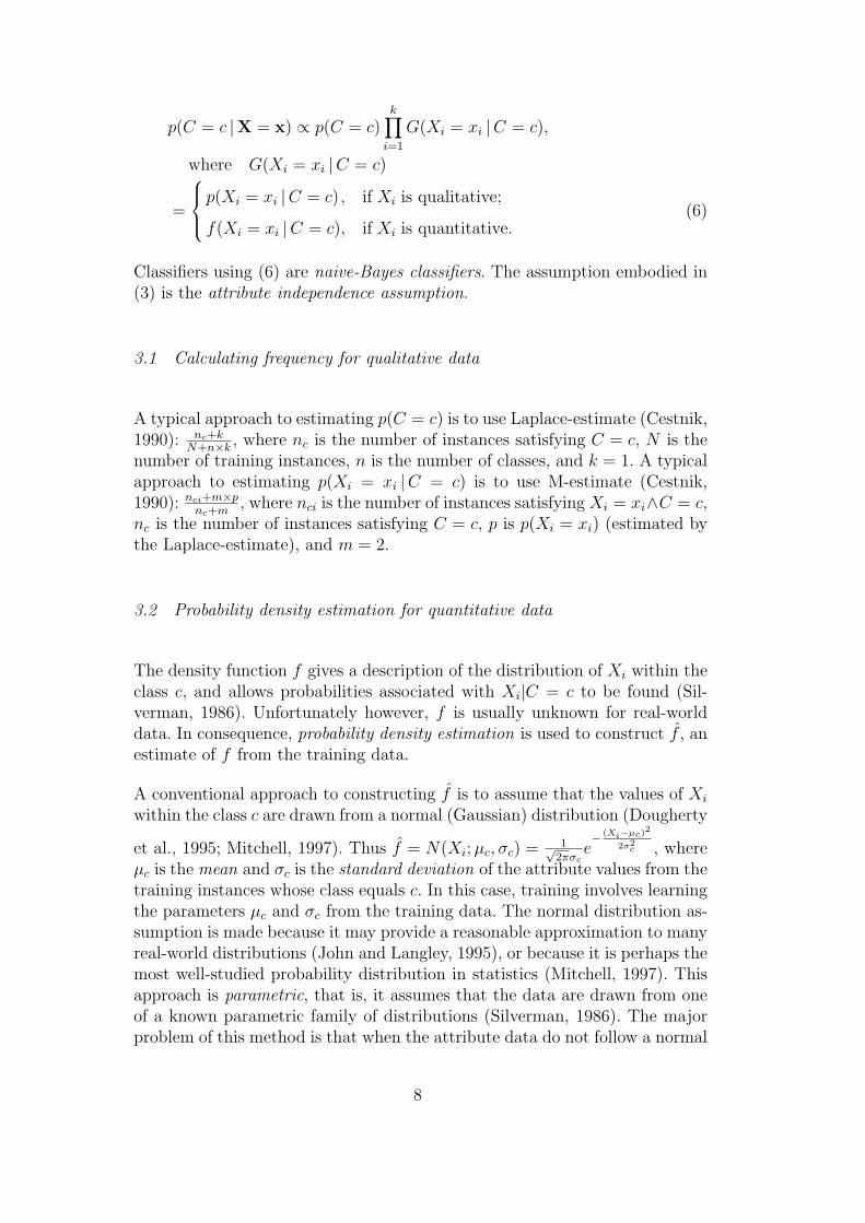
3.2 Probability density estimation for quantitative data

The density function f gives a description of the distribution of Xi within theclass c, and allows probabilities associated with Xi|C = c to be found (Sil-verman, 1986). Unfortunately however, f is usually unknown for real-worlddata. In consequence, probability density estimation is used to construct f̂ , anestimate of f from the training data.

A conventional approach to constructing f̂ is to assume that the values of Xi

within the class c are drawn from a normal (Gaussian) distribution (Dougherty

et al., 1995; Mitchell, 1997). Thus f̂ = N(Xi; µc, σc) = 1√2πσc

e− (Xi−µc)2

2σ2c , where

µc is the mean and σc is the standard deviation of the attribute values from thetraining instances whose class equals c. In this case, training involves learningthe parameters µc and σc from the training data. The normal distribution as-sumption is made because it may provide a reasonable approximation to manyreal-world distributions (John and Langley, 1995), or because it is perhaps themost well-studied probability distribution in statistics (Mitchell, 1997). Thisapproach is parametric, that is, it assumes that the data are drawn from oneof a known parametric family of distributions (Silverman, 1986). The majorproblem of this method is that when the attribute data do not follow a normal

8

distribution, which is often the case in real-world data, the probability esti-mation of naive-Bayes classifiers is not reliable and thus can lead to inferiorclassification performance (Dougherty et al., 1995; Pazzani, 1995).

A second approach is less parametric in that it does not constrain f̂ to fallin a given parametric family. Thus less rigid assumptions are made aboutthe distribution of the observed data (Silverman, 1986). A typical approachis kernel density estimation (John and Langley, 1995). f̂ is averaged over alarge set of Gaussian kernels, f̂ = 1

nc

∑i

N(Xi; µi, σc), where nc is the total

number of training instances with class c, µi is the ith value of Xi within classc, and σc = 1√

nc. It has been demonstrated that kernel density estimation

results in higher naive-Bayes classification accuracy than the former methodin domains that violate the normal distribution assumption, and causes onlysmall decreases in accuracy in domains where the assumption holds. However,this approach tends to incur high computational memory and time. Whereasthe former method can estimate µc and σc by storing only the sum of theobserved xi’s and the sum of their squares, this approach must store everyxi. Whereas the former method only has to calculate N(Xi) once for eachXi = xi |C = c, this approach must perform this calculation nc times. Thus ithas a potential problem that undermines the efficiency of naive-Bayes learning.

3.3 Merits of naive-Bayes classifiers

Naive-Bayes classifiers are simple and efficient. They need only to collect infor-mation about individual attributes, which contrasts to most learning systemsthat must consider attribute combinations. Thus naive-Bayes’ computationaltime complexity is only linear with respect to the amount of the trainingdata. This is much more efficient than the exponential complexity of non-naive Bayes approaches (Yang and Liu, 1999; Zhang et al., 2000). They arealso space efficient. They do not require training data be retained in memoryduring classification and can record all required information using only tablesof no more than two dimensions.

Naive-Bayes classifiers are effective. They are optimal methods of supervisedlearning if the independence assumption holds and the estimates of the re-quired probabilities are accurate. Even when the independence assumption isviolated, their classification performance is still surprisingly good comparedwith other more sophisticated classifiers. One reason for this is because thatthe classification estimation under zero-one loss is only a function of the signof the probability estimation. In consequence, the classification accuracy canremain high even while the probability estimation is poor (Domingos andPazzani, 1997).

9

Naive-Bayes classifiers are robust to noisy data such as irrelevant attributes.They take all attributes into account simultaneously. Hence, the impact ofa misleading attribute can be absorbed by other attributes under zero-oneloss (Hsu et al., 2000).

Naive-Bayes classifiers support incremental training (Rennie, 2000; Roy andMcCallum, 2001; Zaffalon and Hutter, 2002). One can map an existing naive-Bayes classifier and a new training instance to a new naive-Bayes classifierwhich is identical to the classifier that would have been learned from theoriginal data augmented by the new instance. Thus it is trivial to updatea naive-Bayes classifier whenever a new training instance becomes available.This contrasts to the non-incremental methods which must build a new classi-fier from scratch in order to utilize new training data. The cost of incrementalupdate is far lower than that of retraining. Consequently, naive-Bayes clas-sifiers are attractive for classification tasks where the training informationupdates frequently.

4 Discretization

Discretization provides an alternative to probability density estimation whennaive-Bayes learning involves quantitative attributes. Under probability den-sity estimation, if the assumed density is not a proper estimate of the true den-sity, the naive-Bayes classification performance tends to degrade (Doughertyet al., 1995; John and Langley, 1995). Since the true density is usually unknownfor real-world data, unsafe assumptions unfortunately often occur. Discretiza-tion can circumvent this problem. Under discretization, a qualitative attributeX∗

i is formed for Xi. Each value x∗i of X∗i corresponds to an interval (ai, bi]

of Xi. Any original quantitative value xi ∈ (ai, bi] is replaced by x∗i . All rele-vant probabilities are estimated with respect to x∗i . Since probabilities of X∗

i

can be properly estimated from corresponding frequencies as long as there areenough training instances, there is no need to assume the probability densityfunction any more. However, because qualitative data have a lower level ofmeasurement than quantitative data (Samuels and Witmer, 1999), discretiza-tion might suffer information loss.

4.1 Why discretization can be effective

Dougherty et al. (1995) conducted an empirical study to show that naive-Bayes classifiers resulting from discretization achieved lower classification errorthan those resulting from unsafe probability density assumptions. With theseempirical supports, Dougherty et al. suggested that discretization could be

10

effective because they did not make assumptions about the form of the prob-ability distribution from which the quantitative attribute values were drawn.Hsu et al. (2000) proposed a further analysis on this issue, based on an as-sumption that each X∗

i has a Dirichlet prior. Their analysis focused on thedensity function f , and suggested that discretization would achieve optimaleffectiveness by forming x∗i for xi such that p(X∗

i = x∗i |C = c) simulated therole of f(Xi = xi |C = c) by distinguishing the class that gives xi high densityfrom the class that gives xi low density. In contrast, as we will prove in Theo-rem 1, we believe that discretization for naive-Bayes learning should focus onthe accuracy of p(C = c |X∗

i = x∗i ) as an estimate of p(C = c |Xi = xi); andthat discretization can be effective to the degree that p(C = c |X∗ = x∗) isan accurate estimate of p(C = c |X = x), where instance x∗ is the discretizedversion of instance x.

Theorem 1 Assume the first l of k attributes are quantitative and the remain-ing attributes are qualitative. 1 Suppose instance X∗ = x∗ is the discretizedversion of instance X = x, resulting from substituting qualitative attributeX∗

i for quantitative attribute Xi (1 ≤ i ≤ l). If ∀i(p(C = c |Xi = xi) =p(C = c |X∗

i = x∗i )), and the naive-Bayes attribute independence assumption(3) holds, we have p(C = c |X = x) ∝ p(C = c |X∗ = x∗).

Proof: According to Bayes theorem, we have:

p(C = c |X = x)

= p(C = c)p(X = x |C = c)

p(X = x);

since the naive-Bayes attribute independence assumption (3) holds, we con-tinue:

=p(C = c)

p(X = x)

k∏

i=1

p(Xi = xi |C = c);

using Bayes theorem:

=p(C = c)

p(X = x)

k∏

i=1

p(Xi = xi)p(C = c |Xi = xi)

p(C = c)

=p(C = c)

p(C = c)k

∏ki=1 p(Xi = xi)

p(X = x)

k∏

i=1

p(C = c |Xi = xi);

1 In naive-Bayes learning, the order of attributes does not matter. We make thisassumption only to simplify the expression of our proof. This does not at all affectthe theoretical analysis.

11

since the factor∏k

i=1p(Xi=xi)

p(X=x)is invariant across classes:

∝ p(C = c)1−kk∏

i=1

p(C = c |Xi = xi)

= p(C = c)1−kl∏

i=1

p(C = c |Xi = xi)k∏

j=l+1

p(C = c |Xj = xj);

since ∀li=1(p(C = c |Xi = xi) = p(C = c |X∗

i = x∗i )):

= p(C = c)1−kl∏

i=1

p(C = c |X∗i = x∗i )

k∏

j=l+1

p(C = c |Xj = xj);

using Bayes theorem again:

= p(C = c)1−kl∏

i=1

p(C = c)p(X∗i = x∗i |C = c)

p(X∗i = x∗i )

k∏

j=l+1

p(C = c)p(Xj = xj |C = c)

p(Xj = xj)

= p(C = c)

∏li=1 p(X∗

i = x∗i |C = c)∏k

j=l+1 p(Xj = xj |C = c)∏l

i=1 p(X∗i = x∗i )

∏kj=l+1 p(Xj = xj)

;

since the denominator∏l

i=1 p(X∗i = x∗i )

∏kj=l+1 p(Xj = xj) is invariant across

classes:

∝ p(C = c)l∏

i=1

p(X∗i = x∗i |C = c)

k∏

j=l+1

p(Xj = xj |C = c);

since the naive-Bayes attribute independence assumption (3) holds:

= p(C = c)p(X∗ = x∗ |C = c)

= p(C = c |X∗ = x∗)p(X∗ = x∗);

since p(X∗ = x∗) is invariant across classes:

∝ p(C = c |X∗ = x∗). 2

Theorem 1 assures us that as long as the attribute independence assumptionholds, and discretization forms a qualitative X∗

i for each quantitative Xi such

12

that p(C = c |X∗i = x∗i ) = p(C = c |Xi = xi), discretization will result in

naive-Bayes classifiers delivering the same probability estimates as would beobtained if the correct probability density function were employed. Since X∗

i

is qualitative, naive-Bayes classifiers can estimate p(C = c |X = x) withoutassuming any form of the probability density.

Our analysis that focuses on p(C = c |Xi = xi) instead of f(Xi = xi |C = c),is derived from Kononenko’s 1992. However, Kononenko’s analysis requiredthat the attributes be assumed unconditionally independent of each other,which entitles

∏ki=1 p(Xi = xi) = p(X = x). This assumption is much stronger

than the naive-Bayes attribute independence assumption embodied in (3).Thus we suggest that our deduction in Theorem 1 more accurately capturesthe mechanism by which discretization works in naive-Bayes learning.

4.2 What can affect discretization effectiveness

When we talk about the effectiveness of a discretization method, we mean theclassification performance of naive-Bayes classifiers that are trained on datapre-processed by this discretization method. According to Theorem 1, we be-lieve that the accuracy of estimating p(C = c |Xi = xi) by p(C = c |X∗

i = x∗i )takes a key role in this issue. Two influential factors are decision boundariesand the error tolerance of probability estimation. How discretization deals withthese factors can affect the classification bias and variance of generated clas-sifiers, an effect we name discretization bias and variance. According to (6),the prior probability of each class p(C = c) also affects the final choice of theclass. To simplify our analysis, here we assume that each class has the sameprior probability. Thus we can cancel the effect of p(C = c). However, ouranalysis extends straightforwardly to non-uniform cases.

4.2.1 Classification bias and variance

The performance of naive-Bayes classifiers discussed in our study is measuredby their classification error. The error can be partitioned into a bias term, avariance term and an irreducible term (Kong and Dietterich, 1995; Breiman,1996; Kohavi and Wolpert, 1996; Friedman, 1997; Webb, 2000). Bias describesthe component of error that results from systematic error of the learning al-gorithm. Variance describes the component of error that results from randomvariation in the training data and from random behavior in the learning al-gorithm, and thus measures how sensitive an algorithm is to changes in thetraining data. As the algorithm becomes more sensitive, the variance increases.Irreducible error describes the error of an optimal algorithm (the level of noisein the data). Consider a classification learning algorithm A applied to a set

13

(a) High bias, low variance (b) Low bias, high variance

(c) High bias, high variance (d) Low bias, low variance

Fig. 1. Bias and variance in shooting arrows at a target. Bias means that the archersystematically misses in the same direction. Variance means that the arrows arescattered.

S of training instances to produce a classifier to classify an instance x. Sup-pose we could draw a sequence of training sets S1, S2, ..., Sl, each of size m,and apply A to construct classifiers. The error of A at x can be defined as:Error(A,m,x) = Bias(A,m,x)+V ariance(A,m,x)+Irreducible(A, m,x). Thereis often a ‘bias and variance trade-off’ (Kohavi and Wolpert, 1996). All otherthings being equal, as one modifies some aspect of the learning algorithm, itwill have opposite effects on bias and variance.

Moore and McCabe (2002) illustrated bias and variance through shootingarrows at a target, as reproduced in Figure 1. We can think of the perfectmodel as the bull’s-eye on a target, and the algorithm learning from some setof training data as an arrow fired at the bull’s-eye. Bias and variance describewhat happens when an archer fires many arrows at the target. Bias meansthat the aim is off and the arrows land consistently off the bull’s-eye in thesame direction. The learned model does not center about the perfect model.Large variance means that repeated shots are widely scattered on the target.They do not give similar results but differ widely among themselves. A good

14

I1 I2 I3 I5I4

DB2DB1

0.5

1

P(C X

0

)

P(C = c2 )X

1

1 XP(C = c )1

X1

1

0.1 1 20.3

Fig. 2. Probability distribution in one-attribute problem

learning scheme, like a good archer, must have both low bias and low variance.

4.2.2 Decision boundary

This factor in our analysis is inspired by Hsu et al.’s study on discretiza-tion 2000. However, Hsu et al.’s analysis focused on the curve of f(Xi =xi |C = c). Instead, we are interested in the probability p(C = c |Xi = xi).Besides, Hsu et al.’s analysis only addressed one-attribute classification prob-lems, 2 and only suggested that the analysis could be extended to multi-attribute applications without indicating how this might be so. In contrast, weargue that the analysis involving only one attribute differs from that involvingmulti-attributes, since the final choice of the class is decided by the productof each attribute’s probability in the later situation. A decision boundary of aquantitative attribute Xi in our analysis is the value that makes ties amongthe largest probabilities of p(C |X = x) for a test instance x, given the precisevalues of other attributes presented in x.

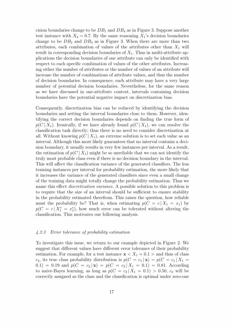
Consider a simple learning task with one quantitative attribute X1 and twoclasses c1 and c2. Suppose X1 ∈ [0, 2], and suppose that the probabilitydistribution function for each class is p(C = c1 |X1) = 1 − (X1 − 1)2 andp(C = c2 |X1) = (X1 − 1)2 respectively, which are plotted in Figure 2. Theconsequent decision boundaries are labelled as DB1 and DB2 respectively inFigure 2. The most-probable class for an instance x =< x1 > changes eachtime x1’s location crosses a decision boundary. Assume a discretization methodto create intervals Ii (i = 1, · · · , 5) as in Figure 2. I2 and I4 contain decisionboundaries while the remaining intervals do not. For any two values in I2

(or I4) but on different sides of a decision boundary, the optimal naive-Bayeslearner under zero-one loss should select a different class for each value. 3 But

2 By default, we talk about quantitative attributes.3 Please note that since naive-Bayes classification is a probabilistic problem, someinstances will be misclassified even when optimal classification is performed. Anoptimal classifier is such that minimizes the naive-Bayes classification error underzero-one loss. Hence even though it is optimal, it still can misclassify instances onboth sides of a decision boundary.

15

0.2

P(C X )2

P(C = c2 )X2

1 XP(C = c )2

DB 1 DB 4

P(C X )1

DB 3DB 2

0X2

1

0.8

0.50.2

0.5

1

0

P(C = c2 )X1 XP(C = c )1

X1

1

1 2

0.7

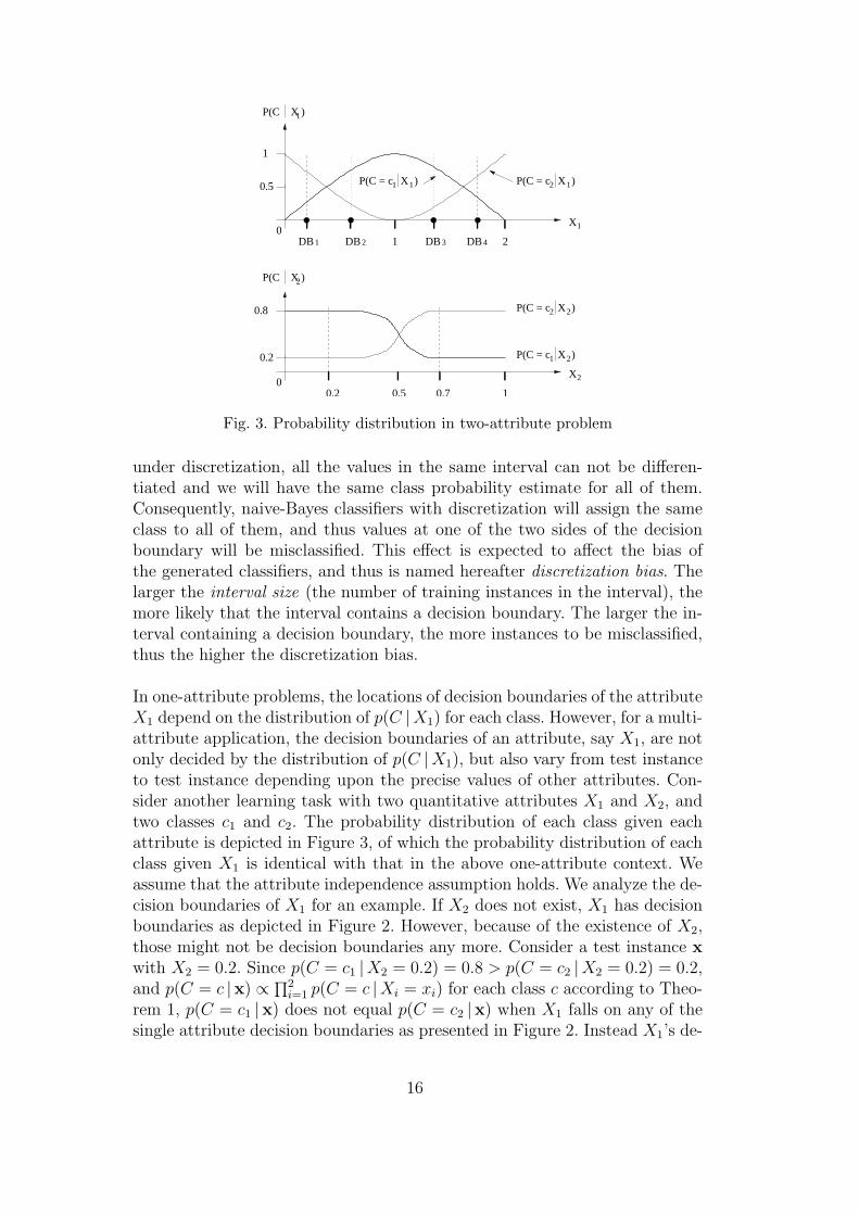
Fig. 3. Probability distribution in two-attribute problem

under discretization, all the values in the same interval can not be differen-tiated and we will have the same class probability estimate for all of them.Consequently, naive-Bayes classifiers with discretization will assign the sameclass to all of them, and thus values at one of the two sides of the decisionboundary will be misclassified. This effect is expected to affect the bias ofthe generated classifiers, and thus is named hereafter discretization bias. Thelarger the interval size (the number of training instances in the interval), themore likely that the interval contains a decision boundary. The larger the in-terval containing a decision boundary, the more instances to be misclassified,thus the higher the discretization bias.

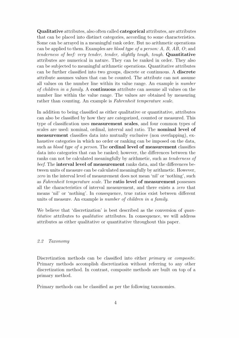
In one-attribute problems, the locations of decision boundaries of the attributeX1 depend on the distribution of p(C |X1) for each class. However, for a multi-attribute application, the decision boundaries of an attribute, say X1, are notonly decided by the distribution of p(C |X1), but also vary from test instanceto test instance depending upon the precise values of other attributes. Con-sider another learning task with two quantitative attributes X1 and X2, andtwo classes c1 and c2. The probability distribution of each class given eachattribute is depicted in Figure 3, of which the probability distribution of eachclass given X1 is identical with that in the above one-attribute context. Weassume that the attribute independence assumption holds. We analyze the de-cision boundaries of X1 for an example. If X2 does not exist, X1 has decisionboundaries as depicted in Figure 2. However, because of the existence of X2,those might not be decision boundaries any more. Consider a test instance xwith X2 = 0.2. Since p(C = c1 |X2 = 0.2) = 0.8 > p(C = c2 |X2 = 0.2) = 0.2,and p(C = c |x) ∝ ∏2

i=1 p(C = c |Xi = xi) for each class c according to Theo-rem 1, p(C = c1 |x) does not equal p(C = c2 |x) when X1 falls on any of thesingle attribute decision boundaries as presented in Figure 2. Instead X1’s de-

16

cision boundaries change to be DB1 and DB4 as in Figure 3. Suppose anothertest instance with X2 = 0.7. By the same reasoning X1’s decision boundarieschange to be DB2 and DB3 as in Figure 3. When there are more than twoattributes, each combination of values of the attributes other than X1 willresult in corresponding decision boundaries of X1. Thus in multi-attribute ap-plications the decision boundaries of one attribute can only be identified withrespect to each specific combination of values of the other attributes. Increas-ing either the number of attributes or the number of values of an attribute willincrease the number of combinations of attribute values, and thus the numberof decision boundaries. In consequence, each attribute may have a very largenumber of potential decision boundaries. Nevertheless, for the same reasonas we have discussed in one-attribute context, intervals containing decisionboundaries have the potential negative impact on discretization bias.

Consequently, discretization bias can be reduced by identifying the decisionboundaries and setting the interval boundaries close to them. However, iden-tifying the correct decision boundaries depends on finding the true form ofp(C |X1). Ironically, if we have already found p(C |X1), we can resolve theclassification task directly; thus there is no need to consider discretization atall. Without knowing p(C |X1), an extreme solution is to set each value as aninterval. Although this most likely guarantees that no interval contains a deci-sion boundary, it usually results in very few instances per interval. As a result,the estimation of p(C |X1) might be so unreliable that we can not identify thetruly most probable class even if there is no decision boundary in the interval.This will affect the classification variance of the generated classifiers. The lesstraining instances per interval for probability estimation, the more likely thatit increases the variance of the generated classifiers since even a small changeof the training data might totally change the probability estimation. Thus wename this effect discretization variance. A possible solution to this problem isto require that the size of an interval should be sufficient to ensure stabilityin the probability estimated therefrom. This raises the question, how reliablemust the probability be? That is, when estimating p(C = c |X1 = x1) byp(C = c |X∗

1 = x∗1), how much error can be tolerated without altering theclassification. This motivates our following analysis.

4.2.3 Error tolerance of probability estimation

To investigate this issue, we return to our example depicted in Figure 2. Wesuggest that different values have different error tolerance of their probabilityestimation. For example, for a test instance x < X1 = 0.1 > and thus of classc2, its true class probability distribution is p(C = c1 |x) = p(C = c1 |X1 =0.1) = 0.19 and p(C = c2 |x) = p(C = c2 |X1 = 0.1) = 0.81. Accordingto naive-Bayes learning, as long as p(C = c2 |X1 = 0.1) > 0.50, c2 will becorrectly assigned as the class and the classification is optimal under zero-one

17

loss. This means, the error tolerance of estimating p(C |X1 = 0.1) can be asbig as 0.81− 0.50 = 0.31. However, for another test instance x < X1 = 0.3 >and thus of class c1, its probability distribution is p(C = c1 |x) = p(C =c1 |X1 = 0.3) = 0.51 and p(C = c2 |x) = p(C = c2 |X1 = 0.3) = 0.49. Theerror tolerance of estimating p(C |X1 = 0.3) is only 0.51− 0.50 = 0.01. In thelearning context of multi-attribute applications, the analysis of the toleranceof probability estimation error is even more complicated. The error toleranceof a value of an attribute affects as well as is affected by those of the values ofthe other attributes since it is the multiplication of p(C = c |Xi = xi) of eachxi that decides the final probability of each class.

The lower the error tolerance a value has, the larger its interval size is preferredfor the purpose of reliable probability estimation. Since all the factors thataffect error tolerance vary from case to case, there can not be a universal, oreven a domain-wide constant that represents the ideal interval size, which thuswill vary from case to case. Further, the error tolerance can only be calculatedif the true probability distribution of the training data is known. If it is notknown, then the best we can hope for is heuristic approaches to managingerror tolerance that work well in practice.

4.3 Summary

By this line of reasoning, optimal discretization can only be performed if theprobability distribution of p(C = c |Xi = xi) for each pair of xi and c, giveneach particular test instance, is known; and thus the decision boundaries areknown. If the decision boundaries are not known, which is often the casefor real-world data, we want to have as many intervals as possible so as tominimize the risk that an instance is classified using an interval containinga decision boundary. By this means we expect to reduce the discretizationbias. On the other hand, however, we want to ensure that the intervals aresufficiently large to minimize the risk that the error of estimating p(C =c |X∗

i = x∗i ) will exceed the current error tolerance. By this means we expectto reduce the discretization variance.

However, when the number of the training instances is fixed, there is a trade-off between interval size and interval number. That is, the larger the intervalsize, the smaller the interval number, and vice versa. Because larger intervalsize can result in lower discretization variance but higher discretization bias,while larger interval number can result in lower discretization bias but higherdiscretization variance, low learning error can be achieved by tuning intervalsize and interval number to find a good trade-off between discretization biasand variance. We argue that there is no universal solution to this problem,that the optimal trade-off between interval size and interval number will vary

18

greatly from test instance to test instance.

These insights reveal that, while discretization is desirable when the true un-derlying probability density function is not available, practical discretizationtechniques are necessarily heuristic in nature. The holy grail of an optimaluniversal discretization strategy for naive-Bayes learning is unobtainable.

5 Review of discretization methods

Here we review six key discretization methods, each of which was eitherdesigned especially for naive-Bayes classifiers or is in practice often usedfor naive-Bayes classifiers. We are particularly interested in analyzing eachmethod’s discretization bias and variance, which we believe illuminating.

5.1 Equal width discretization & Equal frequency discretization

Equal width discretization (EWD) (Catlett, 1991; Kerber, 1992; Doughertyet al., 1995) divides the number line between vmin and vmax into k intervalsof equal width, where k is a user predefined parameter. Thus the intervalshave width w = (vmax − vmin)/k and the cut points are at vmin + w, vmin +2w, · · · , vmin + (k − 1)w.

Equal frequency discretization (EFD) (Catlett, 1991; Kerber, 1992; Doughertyet al., 1995) divides the sorted values into k intervals so that each intervalcontains approximately the same number of training instances, where k is auser predefined parameter. Thus each interval contains n/k training instanceswith adjacent (possibly identical) values. Note that training instances withidentical values must be placed in the same interval. In consequence it is notalways possible to generate k equal frequency intervals.

Both EWD and EFD are often used for naive-Bayes classifiers because oftheir simplicity and reasonably good performance (Hsu et al., 2000). Howeverboth EWD and EFD fix the number of intervals to be produced (decided bythe parameter k). When the training data size is very small, intervals willhave small size and thus tend to incur high variance. When the training datasize is very large, intervals will have large size and thus tend to incur veryhigh bias. Thus we anticipate that they control neither discretization bias nordiscretization variance well.

19

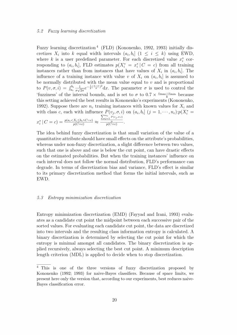
5.2 Fuzzy learning discretization

Fuzzy learning discretization 4 (FLD) (Kononenko, 1992, 1993) initially dis-cretizes Xi into k equal width intervals (ai, bi] (1 ≤ i ≤ k) using EWD,where k is a user predefined parameter. For each discretized value x∗i cor-responding to (ai, bi], FLD estimates p(X∗

i = x∗i |C = c) from all traininginstances rather than from instances that have values of Xi in (ai, bi]. Theinfluence of a training instance with value v of Xi on (ai, bi] is assumed tobe normally distributed with the mean value equal to v and is proportionalto P (v, σ, i) =

∫ biai

1σ√

2πe−

12(x−v

σ)2dx. The parameter σ is used to control the

‘fuzziness’ of the interval bounds, and is set to σ to 0.7 × vmax−vmin

kbecause

this setting achieved the best results in Kononenko’s experiments (Kononenko,1992). Suppose there are nc training instances with known values for Xi andwith class c, each with influence P (vj, σ, i) on (ai, bi] (j = 1, · · · , nc):p(X∗

i =

x∗i |C = c) = p(ai<Xi≤bi∧C=c)p(C=c)

≈∑nc

j=1P (vj,σ,i)

n

p(C=c).

The idea behind fuzzy discretization is that small variation of the value of aquantitative attribute should have small effects on the attribute’s probabilities,whereas under non-fuzzy discretization, a slight difference between two values,such that one is above and one is below the cut point, can have drastic effectson the estimated probabilities. But when the training instances’ influence oneach interval does not follow the normal distribution, FLD’s performance candegrade. In terms of discretization bias and variance, FLD’s effect is similarto its primary discretization method that forms the initial intervals, such asEWD.

5.3 Entropy minimization discretization

Entropy minimization discretization (EMD) (Fayyad and Irani, 1993) evalu-ates as a candidate cut point the midpoint between each successive pair of thesorted values. For evaluating each candidate cut point, the data are discretizedinto two intervals and the resulting class information entropy is calculated. Abinary discretization is determined by selecting the cut point for which theentropy is minimal amongst all candidates. The binary discretization is ap-plied recursively, always selecting the best cut point. A minimum descriptionlength criterion (MDL) is applied to decide when to stop discretization.

4 This is one of the three versions of fuzzy discretization proposed byKononenko (1992; 1993) for naive-Bayes classifiers. Because of space limits, wepresent here only the version that, according to our experiments, best reduces naive-Bayes classification error.

20

Although it has demonstrated strong performance for naive-Bayes (Doughertyet al., 1995; Perner and Trautzsch, 1998), EMD was developed in the contextof top-down induction of decision trees. It uses MDL as the termination con-dition. According to An and Cercone (1999), this has an effect that tendsto form qualitative attributes with few values. We thus anticipate that EMDfocuses on reducing discretization variance, but does not control bias so suc-cessfully. This might work well for training data of small size, for which itis credible that variance reduction can contribute more to lower naive-Bayeslearning error than bias reduction (Friedman, 1997). However, when trainingdata size is large, it is very likely that the loss through bias increase will soonovershadow the gain through variance reduction, resulting in inferior learn-ing performance. Besides since EMD discretizes a quantitative attribute bycalculating the class information entropy as if the naive-Bayes classifiers onlyuse that single attribute after discretization, EMD might be effective at iden-tifying decision boundaries in the one-attribute learning context. But in themulti-attribute learning context, the resulting cut points can easily divergefrom the true ones as we have explained in Section 4.2. If this happens, weanticipate that EMD controls neither bias nor variance well.

5.4 Iterative-improvement discretization

Iterative-improvement discretization (IID) (Pazzani, 1995) initially forms aset of intervals using EWD or EMD, and then iteratively adjusts the intervalsto minimize naive-Bayes classification error on the training data. It definestwo operators: merge two contiguous intervals, and split an interval into twointervals by introducing a new cut point that is midway between each pairof contiguous values in that interval. In each loop of the iteration, for eachquantitative attribute, IID applies all operators in all possible ways to thecurrent set of intervals and estimates the classification error of each adjustmentusing leave-one-out cross validation. The adjustment with the lowest error isretained. The loop stops when no adjustment further reduces the error.

A disadvantage of IID for naive-Bayes learning results from its iterative nature.When the training data size is large, the possible adjustments by applying thetwo operators will tend to be numerous. Consequently the repetitions of theleave-one-out cross validation will be prohibitive so that IID is infeasible interms of computation time. This will impede IID from feasible implementationfor classification tasks with large training data.

IID can split as well as merge discretized intervals. How many intervals willbe formed and where the cut points are located are decided by the error of thecross validation. This is a case by case problem and thus it is not clear whatIID’s systematic impact on bias and variance is. However, if cross-validation is

21

successful in finding a model that minimizing error, then we might infer thatIID can obtain a good discretization bias-variance trade-off.

5.5 Lazy discretization

Lazy discretization (LD) (Hsu et al., 2000) defers discretization until classi-fication time. It waits until a test instance is presented to determine the cutpoints and then estimates probabilities for each quantitative attribute of thetest instance. For each quantitative value from the test instance, it selects apair of cut points such that the value is in the middle of its correspondinginterval and the interval size is equal to that produced by some other algo-rithm chosen by the user. In Hsu et al.’s implementation, the interval size isthe same as created by EFD with k = 10. However, as already noted, 10 is anarbitrary value.

LD tends to have high memory and computational requirements because of itslazy methodology. Eager approaches carry out discretization at training time.Thus the training instances can be discarded before classification time. Incontrast, LD needs to keep the training instances for use during classificationtime. This demands high memory when the training data size is large. Further,where a large number of instances need to be classified, LD will incur largecomputational overheads since it must estimate probabilities from the trainingdata for each instance individually. Although LD achieves comparable accu-racy to EFD and EMD (Hsu et al., 2000), the high memory and computationaloverheads have a potential to damage naive-Bayes classifiers’ classification ef-ficiency. We anticipate that LD’s behavior on discretization bias and variancewill mainly depend on the size strategy of its primary method, such as EFDor EMD.

5.6 Summary

We summarize in Table 1 each previous discretization method in terms of thetaxonomy in Section 2.2.

6 Managing discretization bias and variance

We have argued that the interval size (the number of training instances in aninterval) and interval number (the number of intervals) formed by a discretiza-tion method can affect the method’s discretization bias and variance. Also, a

22

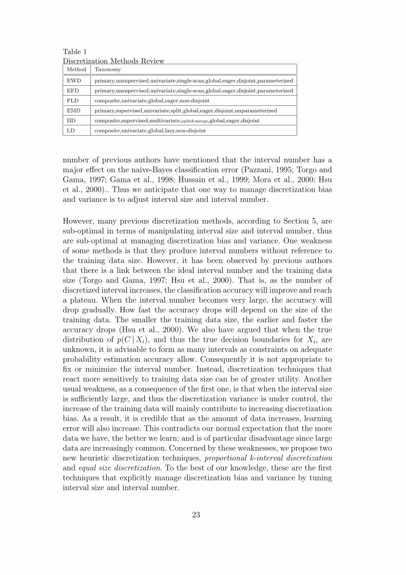
Table 1Discretization Methods Review

Method Taxonomy

EWD primary,unsupervised,univariate,single-scan,global,eager,disjoint,parameterized

EFD primary,unsupervised,univariate,single-scan,global,eager,disjoint,parameterized

FLD composite,univariate,global,eager,non-disjoint

EMD primary,supervised,univariate,split,global,eager,disjoint,unparameterized

IID composite,supervised,multivariate,split&merge,global,eager,disjoint

LD composite,univariate,global,lazy,non-disjoint

number of previous authors have mentioned that the interval number has amajor effect on the naive-Bayes classification error (Pazzani, 1995; Torgo andGama, 1997; Gama et al., 1998; Hussain et al., 1999; Mora et al., 2000; Hsuet al., 2000).. Thus we anticipate that one way to manage discretization biasand variance is to adjust interval size and interval number.

However, many previous discretization methods, according to Section 5, aresub-optimal in terms of manipulating interval size and interval number, thusare sub-optimal at managing discretization bias and variance. One weaknessof some methods is that they produce interval numbers without reference tothe training data size. However, it has been observed by previous authorsthat there is a link between the ideal interval number and the training datasize (Torgo and Gama, 1997; Hsu et al., 2000). That is, as the number ofdiscretized interval increases, the classification accuracy will improve and reacha plateau. When the interval number becomes very large, the accuracy willdrop gradually. How fast the accuracy drops will depend on the size of thetraining data. The smaller the training data size, the earlier and faster theaccuracy drops (Hsu et al., 2000). We also have argued that when the truedistribution of p(C |Xi), and thus the true decision boundaries for Xi, areunknown, it is advisable to form as many intervals as constraints on adequateprobability estimation accuracy allow. Consequently it is not appropriate tofix or minimize the interval number. Instead, discretization techniques thatreact more sensitively to training data size can be of greater utility. Anotherusual weakness, as a consequence of the first one, is that when the interval sizeis sufficiently large, and thus the discretization variance is under control, theincrease of the training data will mainly contribute to increasing discretizationbias. As a result, it is credible that as the amount of data increases, learningerror will also increase. This contradicts our normal expectation that the moredata we have, the better we learn; and is of particular disadvantage since largedata are increasingly common. Concerned by these weaknesses, we propose twonew heuristic discretization techniques, proportional k-interval discretizationand equal size discretization. To the best of our knowledge, these are the firsttechniques that explicitly manage discretization bias and variance by tuninginterval size and interval number.

23

6.1 Proportional k-interval discretization

According to our analysis in Section 4.2, increasing interval size (decreasinginterval number) will decrease variance but increase bias. Conversely, decreas-ing interval size (increasing interval number) will decrease bias but increasevariance. PKID aims to resolve this conflict by setting interval size equalto interval number, and setting both proportional to the number of traininginstances. When discretizing a quantitative attribute for which there are ntraining instances with known values, supposing the desired interval size is sand the desired interval number is t, PKID employs (7) to calculate s and t.It then sorts the quantitative values in ascending order and discretizes theminto intervals of size s. Thus each interval contains approximately s traininginstances with adjacent (possibly identical) values.

s× t = n

s = t. (7)

By setting interval size and interval number equal, PKID equally weighs dis-cretization bias and variance. By setting them proportional to the trainingdata size, PKID can use an increase in training data to lower both discretiza-tion bias and variance. As the number of training instances increases, bothdiscretization bias and variance tend to decrease. Bias can decrease becausethe interval number increases, thus the decision boundaries of the originalquantitative values are less likely to be included in intervals. Variance candecrease because the interval size increases, thus the naive-Bayes probabilityestimation is more stable and reliable. This means that PKID has greatercapacity to take advantage of the additional information inherent in largevolumes of training data than previous methods.

6.2 Equal size discretization

An alternative approach to managing discretization bias and variance is equalsize discretization (ESD). ESD first controls variance. It then uses additionaldata to decrease bias. To discretize a quantitative attribute, ESD sets a safeinterval size m. Then it discretizes the ascendingly sorted values into intervalsof size m. Thus each interval has approximately the same number m of traininginstances with adjacent (possibly identical) values.

By introducing m, ESD aims to ensure that in general the interval size is suf-ficient so that there are enough training instances in each interval to reliablyestimate the naive-Bayes probabilities. Thus ESD can control discretization

24

variance by preventing it from being very high. As we have explained in Sec-tion 4.2, the optimal interval size varies from instance to instance and fromdomain to domain. Nonetheless, we have to choose a size so that we can im-plement and evaluate ESD. In our study, we choose the size as 30 since it iscommonly held to be the minimum sample size from which one should drawstatistical inferences (Weiss, 2002).

By not limiting the number of intervals formed, more intervals can be formedas the training data increases. This means that ESD can make use of extradata to reduce discretization bias. Thus intervals of high bias are not associ-ated with large datasets any more. In this way, ESD can prevent both highbias and high variance.

According to our taxonomy in Section 2.2, both PKID and ESD are unsu-pervised, univariate, single-scan, global, eager and disjoint primary discretiza-tions. PKID is unparameterized, while ESD is parameterized.

7 Time complexity comparison

Here we calculate the time complexities of our new discretization methods aswell as the previous ones discussed in Section 5. Naive-Bayes classifiers arevery attractive to applications with large data because of their computationalefficiency. Thus it will often be important that the discretization methods areefficient so that they can scale to large data.

To discretize a quantitative attribute, suppose the number of training in-stances, 5 test instances, attributes and classes are n, l, v and m respectively.

• EWD, EFD, FLD, PKID and ESD are dominated by sorting. Their com-plexities are of order O(n log n).

• EMD does sorting first, an operation of complexity O(n log n). It then goesthrough all the training instances a maximum of log n times, recursivelyapplying ‘binary division’ to find out at most n−1 cut points. Each time, itwill estimate n − 1 candidate cut points. For each candidate point, proba-bilities of each of m classes are estimated. The complexity of that operationis O(mn log n), which dominates the complexity of the sorting, resulting incomplexity of order O(mn log n).

• IID’s operators have O(n) possible ways to adjust cut points in each itera-tion. For each adjustment, the leave-one-out cross validation has complexityof order O(nmv). The number of times that the iteration will repeat dependson the initial discretization as well the error estimation. It varies from case

5 We only consider instances with known value of the quantitative attribute.

25

to case, which we denote by u here. Thus the complexity of IID is of orderO(n2mvu).

• LD sorts the attribute values once and performs discretization separatelyfor each test instance and hence its complexity is O(n log n) + O(nl).

Thus EWD, EFD, FLD, PKID and ESD have complexity lower than EMD.LD tends to have high complexity when the training or testing data size islarge. IID’s complexity is prohibitively high when the training data size islarge.

8 Experimental evaluation

We evaluate whether PKID and ESD can better reduce naive-Bayes classifica-tion error by better managing discretization bias and variance, compared withprevious discretization methods, EWD, EFD, FLD, EMD and LD. 6 Since IIDtends to have high computational complexity, while our experiments includelarge training data (up to 166 quantitative attributes and up to half milliontraining instances), we do not implement it for the sake of feasibility.

8.1 Data

We ran our experiments on 29 natural datasets from UCI machine learn-ing repository (Blake and Merz, 1998) and KDD archive (Bay, 1999). Thisexperimental suite comprises 3 parts. The first part is composed of all theUCI datasets used by Fayyad and Irani (1993) when publishing the entropyminimization heuristic for discretization. The second part is composed of allthe UCI datasets with quantitative attributes used by Domingos and Pazzani(1996) for studying naive-Bayes classification. In addition, as discretizationbias and variance responds to the training data size and the first two partsare mainly confined to small size, we further augment this collection withdatasets that we can identify containing numeric attributes, with emphasison those having more than 5000 instances. Table 2 describes each dataset,including the number of instances (Size), quantitative attributes (Qa.), quali-tative attributes (Ql.) and classes (C.). The datasets are ordered increasinglyby size.

6 EWD, EFD and FLD are implemented with the parameter k = 10. LD is imple-mented with the interval size equal to that produced by EFD with k = 10.

26

Table 2Experimental Datasets and Classification Error

Classification Error %

Dataset Size Qa. Ql. C.

EWD EFD FLD EMD LD PKID ESD

Labor-Negotiations 57 8 8 2 12.3 8.9 12.8 9.5 9.6 7.4 9.3

Echocardiogram 74 5 1 2 29.6 30.0 26.5 23.8 29.1 25.7 25.7

Iris 150 4 0 3 5.7 7.7 5.4 6.8 6.7 6.4 7.1

Hepatitis 155 6 13 2 14.3 14.2 14.3 13.9 13.7 14.1 15.7

Wine-Recognition 178 13 0 3 3.3 2.4 3.2 2.6 2.9 2.4 2.8

Sonar 208 60 0 2 25.6 25.1 25.8 25.5 25.8 25.7 23.3

Glass-Identification 214 9 0 6 39.3 33.7 40.7 34.9 32.0 32.6 39.1

Heart-Disease(Cleveland) 270 7 6 2 18.3 16.9 15.8 17.5 17.6 17.4 16.9

Liver-Disorders 345 6 0 2 37.1 36.4 37.6 37.4 37.0 38.9 36.5

Ionosphere 351 34 0 2 9.4 10.3 8.7 11.1 10.8 10.4 10.7

Horse-Colic 368 7 14 2 20.5 20.8 20.8 20.7 20.8 20.3 20.6

Credit-Screening(Australia) 690 6 9 2 15.6 14.5 15.2 14.5 13.9 14.4 14.2

Breast-Cancer(Wisconsin) 699 9 0 2 2.5 2.6 2.8 2.7 2.6 2.7 2.6

Pima-Indians-Diabetes 768 8 0 2 24.9 25.6 25.2 26.0 25.4 26.0 26.5

Vehicle 846 18 0 4 38.7 38.8 42.4 38.9 38.1 38.1 38.3

Annealing 898 6 32 6 3.8 2.4 3.7 2.1 2.3 2.1 2.3

German 1000 7 13 2 25.1 25.2 25.2 25.0 25.1 24.7 25.4

Multiple-Features 2000 3 3 10 31.0 31.8 30.9 32.9 31.0 31.2 31.7

Hypothyroid 3163 7 18 2 3.6 2.8 2.7 1.7 2.4 1.8 1.8

Satimage 6435 36 0 6 18.8 18.8 20.2 18.1 18.4 17.8 17.7

Musk 6598 166 0 2 13.7 18.4 23.0 9.4 15.4 8.2 6.9

Pioneer-MobileRobot 9150 29 7 57 13.5 15.0 21.2 19.3 15.3 4.6 3.2

Handwritten-Digits 10992 16 0 10 12.5 13.2 13.3 13.5 12.8 12.0 12.5

Australian-Sign-Language 12546 8 0 3 38.3 37.7 38.7 36.5 36.4 35.8 36.0

Letter-Recognition 20000 16 0 26 29.5 29.8 34.7 30.4 27.9 25.7 25.5

Adult 48842 6 8 2 18.2 18.6 18.5 17.3 18.1 17.1 16.2

Ipums-la-99 88443 20 40 13 21.0 21.1 37.8 21.3 20.4 20.6 18.4

Census-Income 299285 8 33 2 24.5 24.5 24.7 23.6 24.6 23.3 20.0

Forest-Covertype 581012 10 44 7 32.4 33.0 32.2 32.1 32.3 31.7 31.9

ME - - - - 20.1 20.0 21.5 19.6 19.6 18.6 18.6

GE - - - - 16.0 15.6 16.8 15.0 15.3 13.8 13.7

8.2 Design

To evaluate a discretization method, for each dataset, we implement naive-Bayes learning by conducting a 10-trial, 3-fold cross validation. For each fold,the training data are discretized by this method. The intervals so formed areapplied to the test data. The experimental results are recorded as follows.

27

• Classification error, listed under the column ‘Error’ in Table 2, is thepercentage of incorrect classifications of naive-Bayes classifiers in the testaveraged across all folds of the cross validation.

• Classification bias and variance, listed under the columns ‘Bias’ and‘Variance’ respectively in Table 3, are estimated by the method describedby Webb (2000). They equate to the bias and variance defined by Breiman(1996), except that irreducible error is aggregated into bias and variance.An instance is classified once in each trial and hence ten times in all. Thecentral tendency of the learning algorithm is the most frequent classificationof an instance. Total error is the proportional of classifications across the 10trials that are incorrect. Bias is that portion of the total error that is due toerrors committed by the central tendency of the learning algorithm. This isthe portion of classifications that are both incorrect and equal to the centraltendency. Variance is that portion of the total error that is due to errorsthat are deviations from the central tendency of the learning algorithm.This is the portion of classifications that are both incorrect and unequal tothe central tendency. Bias and variance sum to the total error.

8.3 Statistics

Three statistics are employed to evaluate the experimental results.

• Mean error is the arithmetic mean of the errors across all datasets. It pro-vides a gross indication of the relative performance of competitive methods.It is debatable whether errors in different datasets are commensurable, andhence whether averaging errors across datasets is very meaningful. Nonethe-less, a low average error is indicative of a tendency towards low errors forindividual datasets. For each discretization method, the ‘ME’ row in eachtable presents the arithmetic means of the classification error, bias and vari-ance respectively.

• Geometric mean error is the geometric mean of the errors across alldatasets. Webb (2000) suggested that geometric mean error ratio is a moreuseful statistic than mean error ratio across datasets. Geometric mean errorfunctions the same as geometric mean error ratio to indicate the relativeperformance of two methods. For two methods X and Y , the ratio of theirgeometric mean errors is their geometric mean error ratio. That X’s geo-metric mean error is smaller than Y ’s is equivalent to that the geometricmean error ratio of X against Y is smaller than 1, and vice versa. For eachdiscretization method, the ‘GE’ row of each table presents the geometricmeans of the classification error, bias and variance respectively.

• Win/lose/tie record comprises three values that are respectively thenumber of datasets for which the naive-Bayes classifier trained with onediscretization method obtains lower, higher or equal classification error,

28

Table 3Classification Bias and Variance

Classification Bias % Classification Variance %

Dataset Size

EWD EFD FLD EMD LD PKID ESD EWD EFD FLD EMD LD PKID ESD

Labor-Negotiations 57 7.7 5.4 9.6 6.7 6.3 5.1 6.1 4.6 3.5 3.2 2.8 3.3 2.3 3.2

Echocardiogram 74 22.7 22.3 22.0 19.9 22.3 22.4 19.7 6.9 7.7 4.5 3.9 6.8 3.2 5.9

Iris 150 4.2 5.6 4.0 5.0 4.8 4.3 6.2 1.5 2.1 1.4 1.8 1.9 2.1 0.9

Hepatitis 155 13.1 12.2 13.5 11.7 11.8 11.0 14.5 1.2 2.0 0.8 2.2 1.9 3.1 1.2

Wine-Recognition 178 2.4 1.7 2.2 2.0 2.0 1.7 2.1 1.0 0.7 1.0 0.6 0.9 0.7 0.7

Sonar 208 20.6 19.9 21.0 20.0 20.6 19.9 19.5 5.0 5.2 4.9 5.5 5.2 5.8 3.8

Glass-Identification 214 24.6 21.1 29.0 24.5 21.8 19.8 25.9 14.7 12.6 11..7 10.3 10.2 12.8 13.2

Heart-Disease(Cleveland) 270 15.6 14.9 13.9 15.7 16.1 15.5 15.6 2.7 2.0 1.9 1.8 1.5 2.0 1.3

Liver-Disorders 345 27.6 27.5 30.2 25.7 29.6 28.6 27.7 9.5 8.9 7.4 11.7 7.3 10.3 8.8

Ionosphere 351 8.7 9.6 8.2 10.4 10.4 9.3 8.8 0.7 0.7 0.5 0.7 0.5 1.2 1.9

Horse-Colic 368 18.8 19.6 19.3 18.9 19.2 18.5 19.1 1.7 1.2 1.5 1.7 1.6 1..8 1.5

Credit-Screening(Australia) 690 14.0 12.8 13.8 12.6 12.6 12.2 12.9 1.6 1..7 1.5 1.9 1.3 2.1 1.3

Breast-Cancer(Wisconsin) 699 2.4 2.5 2.7 2.5 2.5 2.5 2.4 0.1 0.1 0.1 0.1 0.1 0.1 0.2

Pima-Indians-Diabetes 768 21.5 22.3 23.4 21.2 22.8 21.7 23.0 3.4 3.3 1.8 4.7 2.6 4.3 3.5

Vehicle 846 31.9 31.9 36.0 32.2 32.4 31.8 32.2 6.9 7.0 6.4 6.7 5.7 6.3 6..1

Annealing 898 2.9 1.9 3.2 1.7 1.7 1.6 1.8 0.8 0.5 0.4 0.4 0.6 0.6 0.5

German 1000 21.9 22.1 22.3 21.2 22.3 21.0 21.8 3.1 3.1 2.9 3.8 2.9 3.7 3..6

Multiple-Features 2000 27.6 27.9 27.5 28.6 27.9 27.2 27.3 3.4 3.9 3.4 4.3 3.1 4.0 4.4

Hypothyroid 3163 2.7 2.5 2.5 1.5 2.2 1.5 1.5 0.8 0.3 0.2 0.3 0.2 0.3 0.3

Satimage 6435 18.0 18.3 19.4 17.0 18.0 17.1 16.9 0.8 0.6 0.7 1.1 0.4 0.7 0.8

Musk 6598 13.1 16.9 22.4 8.5 14.6 7.6 6.2 0.7 1.5 0.6 0.9 0.8 0.7 0.6

Pioneer-MobileRobot 9150 11.0 11.8 18.0 16.1 12.9 2.8 1.6 2.5 3.2 3.2 3.2 2.4 1.9 1.7

Handwritten-Digits 10992 12.0 12.3 12.9 12.1 12.1 10.7 10.5 0.5 0.9 0.4 1.4 0.6 1.4 2.0

Australian-Sign-Language 12546 35.8 36.3 36.9 34.0 35.4 34.0 34.1 2.5 1.4 1.8 2.5 1.0 1.8 2.0

Letter-Recognition 20000 23.9 26.5 30.3 26.2 24.7 22.5 22.2 5.5 3.3 4.5 4.2 3.2 3.2 3.3

Adult 48842 18.0 18.3 18.3 16.8 17.9 16.6 15.2 0.2 0.3 0.2 0.5 0.2 0.5 1..0

Ipums-la-99 88443 16.9 17.2 25.1 16.9 16.9 15.9 13.5 4.1 4.0 12.7 4.1 3.5 4.7 4.9

Census-Income 299285 24.4 24.3 24.6 23.3 24.4 23.1 18.9 0.2 0.2 0.2 0.2 0.2 0.2 1.1

Forest-Covertype 581012 32.0 32.5 31.9 31.1 32.0 30.3 29.6 0.4 0.5 0.3 1..0 0.3 1.4 2.3

ME - 17.1 17.2 18.8 16.7 17.2 15.7 15.8 3.0 2.8 2.8 2.9 2.4 2.9 2.8

GE - 13.5 13.2 14.6 12.7 13.2 11.4 11.4 1.7 1.6 1.4 1.7 1.3 1.7 1.8

compared with the naive-Bayes classifier trained with another discretiza-tion method. A one-tailed sign test can be applied to each record. If thetest result is significantly low (here we use the 0.05 critical level), it is rea-sonable to conclude that the outcome is unlikely to be obtained by chanceand hence the record of wins to losses represents a systematic underlyingadvantage to the winning discretization method with respect to the typeof datasets studied. Table 4 presents the records on classification error ofPKID and ESD respectively compared with all the previous discretizationmethods.

29

Table 4Win/lose/tie records of classification error

PKID ESD

Methods

Win Lose Tie Sign Test Win Lose Tie Sign Test

vs. EWD 22 7 0 <0.01 20 8 1 0.02

vs. EFD 22 6 1 <0.01 19 8 2 0.03

vs. FLD 23 6 0 <0.01 22 7 0 <0.01

vs. EMD 21 5 3 <0.01 20 9 0 0.03

vs. LD 20 8 1 0.02 19 8 2 0.03

8.4 Result analysis

According to Table 2, 3 and 4, we have following observations and analysis.

• Both PKID and ESD achieve lower mean and geometric mean of classifi-cation error than all previous methods. With respect to the win/lose/tierecords, both achieve lower classification error than all previous methodswith frequency significant at the 0.05 level. These observations suggest thatPKID and ESD enjoy an advantage in terms of classification error reductionover the type of datasets studied in this research.

• PKID and ESD better reduce classification bias than alternative methods.They both achieve lower mean and geometric mean of classification bias.Their advantage in bias reduction grows more apparent with the trainingdata size increasing. This supports our suggestion that PKID and ESD canuse additional data to decrease discretization bias, and thus high bias doesnot attach to large training data any more.

• PKID’s outstanding performance in bias reduction is achieved without in-curring high variance. This is because PKID equally weighs bias reductionand variance reduction. ESD also demonstrates a good control on discretiza-tion variance. Especially among smaller datasets where naive-Bayes proba-bility estimation has a higher risk to suffer insufficient training data, ESDusually achieves lower variance than alternative methods. This supports oursuggestion that by controlling the size of the interval, ESD can prevent thediscretization variance from being very high. However, we have also ob-served that ESD does have higher variance especially in some very largedatasets. We suggest the reason is that m = 30 might not be the optimalsize for those datasets. Nonetheless, the gain through ESD’s bias reductionis more than the loss through its variance increase, thus ESD still achieveslower naive-Bayes classification error in large datasets.

• Although PKID and ESD manage discretization bias and variance from twodifferent perspectives, they obtain effectiveness competing with each other.The win/lose/tie record of PKID compared with ESD is 15/12/2, which isinsignificant with sign test = 0.35.

30

9 Conclusion

We have proved a theorem that provides a new explanation on why discretiza-tion can be effective for naive-Bayes learning. The theorem states that as longas discretization preserves the conditional probability of each class given eachquantitative attribute value for each test instance, discretization will result innaive-Bayes classifiers delivering the same probability estimates as would beobtained if the correct probability density functions were employed. Two fac-tors that affect discretization’s effectiveness are decision boundaries and the er-ror tolerance of probability estimation for each quantitative attribute. We haveanalyzed the effect of multiple attributes on these factors, and proposed thebias-variance characterisation of discretization. We have demonstrated thatit is unrealistic to expect a single discretization to provide optimal classifica-tion performance for multiple instances. Rather, an ideal discretization schemewould discretize separately for each instance to be classified. Where this is notfeasible, heuristics that manage discretization bias and variance should be em-ployed. In particular, we have obtained new insights into how discretizationbias and variance can be manipulated by adjusting interval size and intervalnumber. In short, we want to maximize the number of intervals in order tominimize discretization bias, but at the same time ensure that each inter-val contains sufficient training instances in order to obtain low discretizationvariance.

These insights have motivated our new heuristic discretization methods, pro-portional k-interval discretization (PKID) and equal size discretization (ESD).Both PKID and ESD are able to actively take advantage of increasing infor-mation in large data to reduce discretization bias and variance. Thus they areexpected to demonstrate greater advantage than previous methods especiallywhen learning from large data.

It is desirable that a machine learning algorithm maximizes the informationthat it derives from large datasets, since increasing the size of a dataset canprovide a domain-independent way of achieving higher accuracy (Freitas andLavington, 1996; Provost and Aronis, 1996). This is especially important sincelarge datasets with high dimensional attribute spaces and huge numbers of in-stances are increasingly used in real-world applications; and naive-Bayes clas-sifiers are particularly attractive to theses applications because of their spaceand time efficiency. Our experimental results have supported our theoreticalanalysis. They have demonstrated that with significant frequency, our newmethods reduce naive-Bayes classification error when compared to previousalternatives. Another interesting issue arising from our study is that unsu-pervised discretization methods are able to outperform supervised ones, inour experiments the entropy minimization discretization (Fayyad and Irani,1993), in the context of naive-Bayes learning. This contradicts the previous

31

understanding that supervised methods tend to have an advantage over un-supervised methods (Dougherty et al., 1995; Hsu et al., 2000).

References

An, A., Cercone, N., 1999. Discretization of continuous attributes for learningclassification rules. In: Proceedings of the Third Pacific-Asia Conference onMethodologies for Knowledge Discovery and Data Mining. pp. 509–514.

Androutsopoulos, I., Koutsias, J., Chandrinos, K., Spyropoulos, C., 2000. Anexperimental comparison of naive Bayesian and keyword-based anti-spamfiltering with encrypted personal e-mail messages. In: Proceedings of the23rd Annual International ACM SIGIR Conference on Research and Devel-opment in Information Retrieval. pp. 160–167.

Bauer, E., Kohavi, R., 1999. An empirical comparison of voting classificationalgorithms: Bagging, boosting, and variants. Machine Learning 36 (1-2),105–139.

Bay, S. D., 1999. The UCI KDD archive [http://kdd.ics.uci.edu]. Depart-ment of Information and Computer Science, University of California, Irvine.

Bay, S. D., 2000. Multivariate discretization of continuous variables for setmining. In: Proceedings of the Sixth ACM SIGKDD International Confer-ence on Knowledge Discovery and Data Mining. pp. 315–319.

Blake, C. L., Merz, C. J., 1998. UCI repository of machine learning databases[http://www.ics.uci.edu/~mlearn/MLRepository.html]. Department ofInformation and Computer Science, University of California, Irvine.

Bluman, A. G., 1992. Elementary Statistics, A Step By Step Approach.Wm.C.Brown Publishers, page5-8.

Breiman, L., 1996. Bias, variance and arcing classifiers. Technical Report,Statistics Department, University of California, Berkeley .

Casella, G., Berger, R. L., 1990. Statistical Inference. Pacific Grove, Calif.Catlett, J., 1991. On changing continuous attributes into ordered discrete at-

tributes. In: Proceedings of the European Working Session on Learning. pp.164–178.

Cestnik, B., 1990. Estimating probabilities: A crucial task in machine learning.In: Proceedings of the Ninth European Conference on Artificial Intelligence.pp. 147–149.

Cestnik, B., Kononenko, I., Bratko, I., 1987. Assistant 86: A knowledge-elicitation tool for sophisticated users. In: Proceedings of the Second Euro-pean Working Session on Learning. pp. 31–45.

Clark, P., Niblett, T., 1989. The cn2 induction algorithm. Machine Learning3, 261–283.

Crawford, E., Kay, J., Eric, M., 2002. Iems - the intelligent email sorter. In:Proceedings of the Nineteenth International Conference on Machine Learn-ing. pp. 83–90.

32

Domingos, P., Pazzani, M., 1996. Beyond independence: Conditions for theoptimality of the simple Bayesian classifier. In: Proceedings of the Thir-teenth International Conference on Machine Learning (ICML’96). MorganKaufmann Publishers, pp. 105–112.

Domingos, P., Pazzani, M., 1997. On the optimality of the simple Bayesianclassifier under zero-one loss. Machine Learning 29, 103–130.

Dougherty, J., Kohavi, R., Sahami, M., 1995. Supervised and unsuperviseddiscretization of continuous features. In: Proceedings of the Twelfth Inter-national Conference on Machine Learning. pp. 194–202.

Fayyad, U. M., Irani, K. B., 1993. Multi-interval discretization of continuous-valued attributes for classification learning. In: Proceedings of the Thir-teenth International Joint Conference on Artificial Intelligence. pp. 1022–1027.

Frasconi, P., Soda, G., Vullo, A., 2001. Text categorization for multi-pagedocuments: a hybrid naive bayes hmm approach. In: Proceedings of theACM/IEEE Joint Conference on Digital Libraries. pp. 11–20.

Freitas, A. A., Lavington, S. H., 1996. Speeding up knowledge discovery inlarge relational databases by means of a new discretization algorithm. In:Advances in Databases, Proceedings of the Fourteenth British National Con-ferenc on Databases. pp. 124–133.

Friedman, J. H., 1997. On bias, variance, 0/1-loss, and the curse-of-dimensionality. Data Mining and Knowledge Discovery 1 (1), 55–77.

Gama, J., 2000. Iterative Bayes. Intelligent Data Analysis 4, 475–488.Gama, J., Torgo, L., Soares, C., 1998. Dynamic discretization of continuous

attributes. In: Proceedings of the Sixth Ibero-American Conference on AI.pp. 160–169.

Guthrie, L., Walker, E., 1994. Document classification by machine: Theoryand practice. In: Proceedings of COLING-94.

Hsu, C. N., Huang, H. J., Wong, T. T., 2000. Why discretization works fornaive Bayesian classifiers. In: Proceedings of the Seventeenth InternationalConference on Machine Learning. pp. 309–406.

Hussain, F., Liu, H., Tan, C. L., Dash, M., 1999. Discretization: An enablingtechnique. Technical Report, TRC6/99, School of Computing, National Uni-versity of Singapore.

Joachims, T., 1997. A probabilistic analysis of the rocchio algorithm with tfidffor text categorization. In: Proceedings of the International Conference onMachine Learning.

John, G. H., Langley, P., 1995. Estimating continuous distributions inBayesian classifiers. In: Proceedings of the Eleventh Conference on Uncer-tainty in Artificial Intelligence. pp. 338–345.

Kalt, T., 1996. A new probabilistic model of text classification and retrieval.Technical Report IR-78, Center for Intelligent Information Retrieval, Uni-versity of Massachusetts.

Kerber, R., 1992. Chimerge: Discretization for numeric attributes. In: NationalConference on Artificial Intelligence. AAAI Press, pp. 123–128.

33

Kim, Y.-H., Hahn, S.-Y., Zhang, B.-T., 2000. Text filtering by boosting naiveBayes classifiers. In: Proceedings of the 23rd Annual International ACMSIGIR Conference on Research and Development in Information Retrieval.pp. 168–175.

Kohavi, R., 1996. Scaling up the accuracy of naive-Bayes classifiers: a decision-tree hybrid. In: Proceedings of the Second International Conference onKnowledge Discovery and Data Mining.

Kohavi, R., Sommerfield, D., Dougherty, J., 1997. Data mining using MLC++:A machine learning library in C++. International Journal on Artificial In-telligence Tools 6 (4), 537–566.

Kohavi, R., Wolpert, D., 1996. Bias plus variance decomposition for zero-one loss functions. In: Proceedings of the 13th International Conference onMachine Learning. pp. 275–283.

Koller, D., Sahami, M., 1997. Hierarchically classifying documents using veryfew words. In: Proceedings of the Fourteenth International Conference onMachine Learning. pp. 170–178.

Kong, E. B., Dietterich, T. G., 1995. Error-correcting output coding correctsbias and variance. In: Proceedings of the Twelfth International Conferenceon Machine Learning. pp. 313–321.

Kononenko, I., 1990. Comparison of inductive and naive Bayesian learningapproaches to automatic knowledge acquisition.

Kononenko, I., 1992. Naive Bayesian classifier and continuous attributes. In-formatica 16 (1), 1–8.

Kononenko, I., 1993. Inductive and Bayesian learning in medical diagnosis.Applied Artificial Intelligence 7, 317–337.

Kononenko, I., 2001. Machine learning for medical diagnosis: history, state ofthe art and perspective. Artificial Intelligence in Medicine 23 (1), 89–109.

Kukar, M., Groselj, C., Kononenko, I., Fettich, J., 1997. An application ofmachine learning in the diagnosis of ischaemic heart disease. In: Proceedingsof the 6th Conference on Artificial Intelligence in Medicine Europe. pp. 461–464.

Langley, P., Iba, W., Thompson, K., 1992. An analysis of bayesian classifiers.In: Proceedings of the Tenth National Conference on Artificial Intelligence.pp. 223–228.

Larkey, L. S., Croft, W. B., 1996. Combining classifiers in text categorization.In: Proceedings of the 19th Annual International Conference on Researchand Development in Information Retrieval. pp. 289–297.

Lavrac, N., 1998. Data mining in medicine: Selected techniques and applica-tions. In: Proceedings of the Second International Conference on The Prac-tical Applications of Knowledge Discovery and Data Mining. pp. 11–31.

Lavrac, N., Keravnou, E., Zupan, B., 2000. Intelligent data analysis inmedicine. Encyclopedia of Computer Science and Technology 42 (9), 113–157.

Lewis, D. D., 1992. An evaluation of phrasal and clustered representations ona text categorization task. In: Proceedings of the 15th Annual International

34

ACM SIGIR Conference on Research and Development in Information Re-trieval. pp. 37–50.

Lewis, D. D., 1998. Naive (Bayes) at forty: The independence assumption ininformation retrieval. In: In European Conf. on Machine Learning.

Lewis, D. D., Gale, W. A., 1994. A sequential algorithm for training textclassifiers. In: Proceedings of the 17th Annual International ACM-SIGIRConference on Research and Development in Information Retrieval. pp. 3–12.

Li, H., Yamanishi, K., 1997. Document classification using a finite mixturemodel. In: Proceedings of the 8th Conference of the European Chapter ofthe Association for Computational Linguistics. pp. 39–47.

Maron, M., 1961. Automatic indexing: An experimental inquiry. Journal ofthe Association for Computing Machinery 8, 404–417.

Maron, M., Kuhns, J., 1960. On relevance, probabilistic indexing, and infor-mation retrieval. Journal of the Association for Computing Machinery 7 (3),216–244.

McCallum, A., Nigam, K., 1998. A comparison of event models for naive bayestext classification. In: Proceedings of the AAAI-98 Workshop on Learningfor Text Categorization.

McCallum, A., Rosenfeld, R., Mitchell, T. M., Ng, A., 1998. Improving textclassification by shrinkage in a hierarchy of classes. In: Proceedings of the15th International Conference on Machine Learning.

McSherry, D., 1997a. Avoiding premature closure in sequential diagnosis. Ar-tificial Intelligence in Medicine 10 (3), 269–283.

McSherry, D., 1997b. Hypothesist: A development environment for intelligentdiagnostic systems. In: Proceedings of the 6th Conference on Artificial In-telligence in Medicine in Europe. pp. 223–234.

Mitchell, T. M., 1997. Machine Learning. McGraw-Hill Companies.Miyahara, K., Pazzani, M. J., 2000. Collaborative filtering with the simple

bayesian classifier. In: Proceedings of the 6th Pacific Rim International Con-ference on Artificial Intelligence. pp. 679–689.

Montani, S., Bellazzi, R., Portinale, L., Fiocchi, S., Stefanelli, M., 1998. A case-bbased retrieval system for diabetic patient therapy. IDAMAP 98 workingnotes.

Mooney, R. J., Roy, L., 2000. Content-based book recommending using learn-ing for text categorization. In: Proceedings of DL-00, 5th ACM Conferenceon Digital Libraries. ACM Press, New York, US, San Antonio, US, pp. 195–204.

Moore, D. S., McCabe, G. P., 2002. Introduction to the Practice of Statistics.Michelle Julet, fourth Edition.

Mora, L., Fortes, I., Morales, R., Triguero, F., 2000. Dynamic discretizationof continuous values from time series. In: Proceedings of the Eleventh Eu-ropean Conference on Machine Learning. pp. 280–291.

Nigam, K., McCallum, A., Thrun, S., Mitchell, T. M., 1998. Learning to clas-sify text from labeled and unlabeled documents. In: Proceedings of the Fif-

35

teenth National Conference on Artificial Intelligence and Tenth InnovativeApplications of Artificial Intelligence Conference, AAAI 98, IAAI 98. pp.792–799.

Pantel, P., Lin, D., 1998. Spamcop a spam classification & organization pro-gram. In: Proceedings of AAAI-98 Workshop on Learning for Text Catego-rization. pp. 95–98.

Pazzani, M., Billsus, D., 1997. Learning and revising user profiles: The iden-tification of interesting web sites. Machine Learning 27 , 313–331.

Pazzani, M., Muramatsu, J., Billsus, D., 1996. Syskill & webert: Identifying in-teresting web sites. In: Proceedings of the National Conference on ArtificialIntelligence.

Pazzani, M. J., 1995. An iterative improvement approach for the discretizationof numeric attributes in Bayesian classifiers. In: Proceedings of the FirstInternational Conference on Knowledge Discovery and Data Mining.

Perner, P., Trautzsch, S., 1998. Multi-interval discretization methods for de-cision tree learning. In: Advances in Pattern Recognition, Joint IAPR In-ternational Workshops SSPR ’98 and SPR ’98. pp. 475–482.

Provost, F. J., Aronis, J. M., 1996. Scaling up machine learning with massiveparallelism. Machine Learning 23.

Provost, J., 1999. Naive-Bayes vs. rule-learning in classification of email. Tech-nical Report AI-TR-99-284, Artificial Intelligence Lab, The University ofTexas at Austin.

Quinlan, J. R., 1993. C4.5: Programs for Machine Learning. Morgan Kauf-mann Publishers.

Rennie, J., 2000. ifile: An application of machine learning to mail filtering. In:Proceedings of the KDD-2000 Workshop on Text Mining.

Roy, N., McCallum, A., 2001. Toward optimal active learning through sam-pling estimation of error reduction. In: Proceedings of the Eighteenth Inter-national Conference on Machine Learning. pp. 441–448.

Samuels, M. L., Witmer, J. A., 1999. Statistics For The Life Sciences, SecondEdition. Prentice-Hall, page10-11.

Scheaffer, R. L., McClave, J. T., 1995. Probability and Statistics for Engineers,4th Edition. Duxbury Press.

Silverman, B., 1986. Density Estimation for Statistics and Data Analysis.Chapman and Hall Ltd.

Starr, B., Ackerman, M. S., Pazzani, M., 1996a. Do i care? – tell me what’schanged on the web. AAAI Spring Symposium. Stanford, CA.

Starr, B., Ackerman, M. S., Pazzani, M., 1996b. Do-i-care: A collaborativeweb agent. In: Proceedings of the ACM Conference on Human Factors inComputing Systems. pp. 273–274.

Ting, K., Zheng, Z., 1999. Improving the performance of boosting for naiveBayesian classification. In: Proceedings of the Third Pacific-Asia Conferenceon Knowledge Discovery and Data Mining. pp. 296–305.

Torgo, L., Gama, J., 1997. Search-based class discretization. In: Proceedingsof the Ninth European Conference on Machine Learning. pp. 266–273.

36

Tsymbal, A., Puuronen, S., Patterson, D., 2002. Feature selection for ensem-bles of simple bayesian classifiers. In: Proceedings of the 13th InternationalSymposium on Foundations of Intelligent Systems. pp. 592–600.

Webb, G. I., 2000. Multiboosting: A technique for combining boosting andwagging. Machine Learning 40 (2), 159–196.

Weiss, N. A., 2002. Introductory Statistics. Vol. Sixth Edition. Greg Tobin.Yang, Y., Liu, X., 1999. A re-examination of text categorization methods. In:

Proceedings of ACM SIGIR Conference on Research and Development inInformation Retrieval (SIGIR1999). pp. 42–49.

Zaffalon, M., Hutter, M., 2002. Robust feature selection using distributions ofmutual information. In: Proceedings of the Fourteenth International Con-ference on Uncertainty in Artificial Intelligence.

Zelic, I., Kononenko, I., Lavrac, N., Vuga, V., 1997. Induction of decision treesand bayesian classification applied to diagnosis of sport injuries. Journal ofMedical Systems 21 (6), 429–444.

Zhang, H., Ling, C. X., Zhao, Z., 2000. The learnability of naive Bayes. In:Proceedings of Canadian Artificial Intelligence Conference. pp. 432–441.

Zheng, Z., 1998. Naive Bayesian classifier committees. In: Proceedings of the10th European Conference on Machine Learning. pp. 196–207.

Zupan, B., Demsar, J., Kattan, M. W., Ohori, M., Graefen, M., Bohanec, M.,Beck, J. R., 2001. Orange and decisions-at-hand: Bridging predictive datamining and decision support. In: Proceedings of IDDM2001: ECML/PKDD-2001 Workshop on Integrating Aspects of Data Mining, Decision Supportand Meta-Learning. pp. 151–162.

37